arX

iv:0

911.

1032

v1 [

mat

h-ph

] 5

Nov

200

9

Rigorous meaning of McLennan ensembles

Christian Maes1 and Karel Netocny2

1Instituut voor Theoretische Fysica, K.U.Leuven, Belgium∗

2Institute of Physics AS CR, Prague, Czech Republic†

We analyze the exact meaning of expressions for nonequilibrium stationary distri-

butions in terms of entropy changes. They were originally introduced by McLennan

for mechanical systems close to equilibrium and more recent work by Komatsu and

Nakagawa has shown their intimate relation to the transient fluctuation symmetry.

Here we derive these distributions for jump and diffusion Markov processes and we

clarify the order of the limits that take the system both to its stationary regime

and to the close-to-equilibrium regime. In particular, we prove that it is exactly the

(finite) transient component of the irreversible part of the entropy flux that corrects

the Boltzmann distribution to first order in the driving. We add further connections

with the notion of local equilibrium, with the Green-Kubo relation and with a gen-

eralized expression for the stationary distribution in terms of a reference equilibrium

process.

I. INTRODUCTION

According to McLennan [20, 21], the stationary density of an open mechanical system

away but close to thermal equilibrium can be written in the modified Gibbs form

ρ(x) ≃1

Ze−βH(x)+W (x) (I.1)

with the nonequilibrium correction W directly related to the entropy production or to the

dissipation in the driven system. An essential feature of the formula, not quite visible yet, is

that the distribution ρ is described in terms of macroscopic parameters only, such as external

temperature and driving fields. It was also expected “that some formal advantages may be

∗Electronic address: christian.maes@fys.kuleuven.be†Electronic address: netocny@fzu.cz

2

offered by an approach to nonequilibrium phenomena in which the Gibbs ensemble plays a

more prominent role” (from the second paragraph in [20]). Because of the suggested physical

interpretation, this proposal opens the possibility to construct nonequilibrium statistical

ensembles based on meaningful physical quantities, see also [11, 12] for older and [22] for

more recent work. However, (I.1) in [20] being just the result of a formal perturbation

calculation (together with some projection techniques), there have remained a number of

difficulties with the exact meaning of this proposal as well as with its scope of generality.

We mention some of these problems, as are clarified in the present paper:

(1) What entropy production does the correction term W represent?—It can only be

some transient component of the total entropy production as the total entropy production

clearly diverges in the long-time (stationary) limit. Moreover, this divergence (equal to the

steady entropy flux) is in fact of order O(ε2) in some ‘distance of equilibrium’ ε since it

comes from the product of thermodynamical forces and fluxes, both being O(ε). The point

will be that the transient irreversible part of the entropy production and its linear part are

both finite: they coincide up to O(ε) and give a valid first-order correction to the Boltzmann

distribution as in (I.1).

(2) Is the proposal also valid on different levels of description than for mechanical

systems?—The formal perturbation approach as in [20] does not reveal the essence and

the physical generality of the proposal. Here the insight comes from dynamical fluctua-

tion theory: formula (I.1) is basically a consequence of the transient fluctuation symmetry,

[8]. In other words, it follows from the local detailed balance assumption which determines

the time-antisymmetric structure of the space-time distribution in terms of the history-

dependent entropy fluxes, cf. [13, 14]. We make that visible for Markov processes.

(3) Can one go beyond close-to-equilibrium?—As explained in [8] and further applied

in [9, 10], one can in principle obtain a formal perturbation series for the stationary distri-

bution based on (all) the cumulants of the transient entropy production. An interpretation

has been given for the second-order expansion where the divergences cancel out by a

different way than explained in the present paper. We instead present a generalization

involving the so called dynamical activity or traffic, an advantage being that the evaluation

is now from the start to be done under a reference equilibrium process.

We consider Markov processes of two types, jump and diffusion processes. Yet for sim-

3

plicity we reserve the next section to Markov jump processes; the diffusion case is formally

completely similar. We explain the relation with local equilibrium in Section IID. In Sec-

tion III we make some specific remarks on the diffusion case and we also take there the

opportunity to illustrate an alternative to the derivation in Section IIB. As an application,

the Green-Kubo relations are derived in Section IIIB. An illustration of the McLennan-

algorithm for an underdamped case is given in Section IIIC. We end, in Section IV, with a

generalization away from equilibrium.

II. MARKOV JUMP PROCESSES

After introducing some notation and basic concepts in the case of jump processes, we

give our main result which is a rigorous version of the McLennan formula. A comparison to

another approach and further remarks are added.

A. Set-up and assumptions

Consider a continuous time Markov proces xt, t ≥ 0, taking values in a finite state space

Ω ∋ x, y, . . .. The transition rates are λ(x, y) ≥ 0 for jumps between the states x → y. The

Master equation for the probability µt(x) of state x as function of time t is

dµt(x)

dt=

∑

y 6=x

µt(y)λ(y, x)− µt(x)λ(x, y) (II.1)

with some given initial law µ0 = µ at time zero.

Physical input distinguishes between equilibrium and nonequilibrium dynamics. An equi-

librium dynamics (with subscript 0) satisfies the condition of detailed balance, i.e.,

ρ0(x) λ0(x, y) = ρ0(y) λ0(y, x) (II.2)

where ρ0(x) ∝ e−βU(x) for some potential U and inverse temperature β, is then stationary.

This relation expresses the time-reversibility of the stationary equilibrium process. For

nonequilibrium systems, detailed balance (II.2) gets broken. An extension is known as the

condition of local detailed balance. In terms of a potential U(x) and a work function (or

driving) F (x, y) = −F (y, x), the rates now satisfy

λ(x, y) = eβ [F (x,y)+U(x)−U(y)] λ(y, x) (II.3)

4

where β ≥ 0 can still be interpreted as the inverse temperature of a reference reservoir, but

that is not necessary except for setting the right units.

We can rewrite the local detailed balance condition (II.3) as

ρ0(x)λ(x, y) = γ(x, y) eβ

2F (x,y) (II.4)

for a symmetric γ(x, y) = γ(y, x), which here is arbitrary.

In the present paper we are concerned with the close-to-equilibrium regime where F

is small. To make it precise, we parameterize the distance to equilibrium explicitly by

assuming that γ(x, y) = γε(x, y) and F (x, y) = Fε(x, y) (and hence also λ(x, y) = λε(x, y))

depend on a parameter ε ∈ [0, ε0]. With no loss of generality we let Fε(x, y) = εF1(x, y).

As becomes obvious later, the ε−dependence of γε(x, y) is irrelevant for the first-order

calculations.

We also consider the probability of trajectories, or rather, how to obtain probability

densities in path-space. For this we start with a probability law µ at time zero for the

Markov process, and write Pµ for its path-space distribution over a time interval [0, T ].

That has a density with respect to the corresponding stationary equilibrium process P0

with rates λ0(x, y) and starting from ρ0, explicitly given by the Girsanov formula

dPµ

dP0

(ω) =µ(x0)

ρ0(x0)exp

−

∫ T

0

(

ξ(xt) − ξ0(xt))

dt +∑

0<t≤T

logλ(xt− , xt)

λ0(xt− , xt)

(II.5)

where ω = (xt)Tt=0, xt ∈ Ω, is a piecewise constant right-continuous trajectory, with the

escape rates

ξ(x) =∑

y 6=x

λ(x, y)

and with the last sum in the exponent being over the jump times t where the state changes

from xt− to xt. Mathematical details are found in, e.g., Appendix 2 of [7].

From (II.5), the path-space action A in

dPµ(ω) = dP0(ω)µ(x0)

ρ0(x0)e−A(ω) (II.6)

equals

A(ω) = exp

∫ T

0

(

ξ(xt) − ξ0(xt))

dt −∑

0<t≤T

logλ(xt− , xt)

λ0(xt− , xt)

5

As a result, its time-antisymmetric part is

STIRR

(ω) = A(θω) − A(ω)

= β∑

0<t≤T

F (xt− , xt) (II.7)

where the time-reversal is the right-continuous modification of θω = (xT−t)Tt=0 for any

ω = (xt)Tt=0. We have used that the first integral in the exponent of (II.5) is time-symmetric,

and that (II.2)–(II.4) combine to produce the forcing in the sum over jump times. We

recognize the resulting STIRR

(ω) as the ‘irreversible’ part in the entropy flux as function of the

path ω. Note that the pathwise relation (II.7) between the time-reversal symmetry breaking

and the entropy flux is a consequence of condition (II.3). For general arguments see e.g. [18].

The mean value of that irreversible part of the entropy production is obtained by taking

the average of (II.7) with respect to our process, using its Markov property:

〈STIRR

〉µ =

∫

dPµ(ω) STIRR

(ω) =

∫ T

0

dt limτ↓0

1

τ〈Sτ

IRR〉µt

= β

∫ T

0

dt∑

x

µt(x)∑

y 6=x

λε(x, y) Fε(x, y)

= β

∫ T

0

dt⟨

∑

y 6=x

λε(xt, y) Fε(xt, y)⟩

µ

(II.8)

Hence, for fixed T we have to first order in ε,

〈STIRR

〉µ = εβ

∫ T

0

dt⟨

w1(xt)⟩0

µ+ O(ε2) (II.9)

where the averaging 〈·〉0µ is now over the equilibrium reference process started from µ, and

w1(x) =∑

y 6=x

λ0(x, y) F1(x, y) (II.10)

is the linear term in the mean entropy flux when at state x.

B. McLennan formula

To be explicit about the various dependencies, we write ρεT for the ε−dependent solution

at time T to the Master equation (II.1), started from the equilibrium law µ0 = ρ0. The

6

smoothness of the deformation is assumed uniformly in time T , and we write ρε = limT ρεT .

We also denote the stationary entropy flux by σε; it is given as

σε =1

T〈ST

IRR〉ρε

= β∑

x

ρε(x)∑

y 6=x

λε(x, y)Fε(x, y)

=β

2

∑

x,y

[ρε(x)λε(x, y) − ρε(y)λε(y, x)] Fε(x, y)

=εβ

2

∑

x,y

γ0(x, y)[ρε(x)

ρ0(x)−

ρε(y)

ρ0(y)

]

F1(x, y) + o(ε2) (II.11)

independently of time span T . We finally recall the linear term w1 from (II.10).

Theorem II.1. Suppose that the equilibrium process (II.2) is irreducible. The following

limiting identities are verified:

limT↑+∞

limε→0

1

εlog

ρεT (x)

ρ0(x)= lim

ε→0lim

T↑+∞

1

εlog

ρεT (x)

ρ0(x)(II.12)

= −β

∫ +∞

0

dt 〈w1(xt)〉0x (II.13)

Moreover,

εβ

∫ +∞

0

dt 〈w1(xt)〉0x = lim

T↑+∞

[

〈STIRR

〉x − σεT]

+ O(ε2) (II.14)

Remark II.2. According to the above result, the stationary distribution has the form

ρε(x) = ρ0(x) exp

−εβ

∫ +∞

0

dt 〈w1(xt)〉0x + O(ε2)

= ρ0(x) exp

limT↑+∞

[

σεT − 〈STIRR

〉x]

+ O(ε2)

(II.15)

which is consistent with the original McLennan’s proposal (I.1) in the sense that it identifies

the correction term W as the transient part of the ‘irreversible’ entropy production for the

process started from state x. Notice that this transient part is O(ε), in contrast to the

stationary entropy production rate which is O(ε2); the latter being also the leading order of

the long-time divergence that needs to be removed. Hence, loosely speaking, the McLennan

proposal is all correct for close-to-equilibrium processes provided that the divergence present

in higher orders in ε is killed by a suitable counterterm.

Proof. The first equality (II.12) follows from the irreducibility of the reference equilibrium

process. The ε−dependent process is obtained by its smooth deformation, see (II.3)–(II.4).

Therefore, ρεT → ρε uniformly in ε ∈ [0, ε1] with some 0 < ε1 ≤ ε0.

7

In order to prove the equality (II.13), the point of departure is the transient fluctuation

symmetry. The formula (II.6) obviously implies

dPρ0(ω) = dP0(ω) e−A(ω)

when starting (in the left-hand side) the nonequilibrium process from the equilibrium law

ρ0. Since the equilibrium process P0 is time-reversal invariant, we have for (II.7)

STIRR

(ω) = logdPρ0

dPρ0θ(ω)

and hence, for all functions f on path-space,

〈f〉ρ0= 〈fθ exp(−ST

IRR)〉ρ0

(II.16)

That is an exact (for all finite times T ) fluctuation symmetry. Take in (II.16) f(ω) = δxT =x,

the Kronecker-delta function equal one if the trajectory ends up at state x and zero otherwise.

We get

ρεT (x) = ρ0(x) 〈e−ST

IRR 〉x (II.17)

where the right-hand side averages over the nonequilibrium process started from the state

x. We substitute (II.7) and we use that the Poisson number of jumps has all exponential

moments, to expand the exponential in (II.17). Using (II.8), it is then easy to verify that

limε↓0

1

εlog〈e−ST

IRR 〉x = −β⟨

∫ T

0

dt w1(xt)⟩0

x(II.18)

which has a limit as T ↑ +∞ since, uniformly in the initial x, the equilibrium process relaxes

exponentially fast to its stationary law for which∑

x ρ0(x)w1(x) = 0 by (II.2). That proves

formula (II.13).

We now turn to (II.14). For all initial laws µ,

〈STIRR

〉µ − σεT = β

∫ T

0

dt∑

x

[µt(x) − ρε(x)]∑

y 6=x

λε(x, y)Fε(x, y)

has a limit T ↑ +∞. Since all terms are uniformly bounded, we can here freely exchange

the limits T ↑ +∞ and ε ↓ 0. The T−limit has leading order in ε, for ε ↓ 0,

εβ

∫ +∞

0

dt∑

x

[µ0t (x) − ρ0(x)]

∑

y 6=x

λ0(x, y)F1(x, y)

= εβ

∫ +∞

0

dt∑

x

µ0t (x)

∑

y 6=x

λ0(x, y)F1(x, y) (II.19)

because F1(x, y) is antisymmetric and ρ0(x)λ0(x, y) is symmetric under x ↔ y. That proves

(II.14).

8

C. Variations

What is mostly new about the above arguments is the point of departure (II.16), which

naturally links McLennan’s correction to the ‘irreversible’ entropy production, cf. [8].

There are other schemes that do not have this advantage; still they can be applied to obtain

systematic corrections to the equilibrium distribution. We discuss one such a formulation

and we apply it to obtain a different perturbation scheme not having an interpretation in

terms of the entropy production.

By using the fundamental theorem of calculus, the stationary measure ρε = ρ can be

obtained in the form

ρ(x) = ρ0(x) +

∫ +∞

0

dt etL⋆

L⋆ρ0(x) (II.20)

for initial law ρ0 and with L⋆µ(x) =∑

y 6=x[λ(y, x)µ(y)− λ(x, y)µ(x)] the forward generator

of the Markov jump process under consideration. Then, from (II.4),

L⋆ρ0(x) = ρ0(x) h(x), h(x) =∑

y 6=x

λ(x, y)[e−βF (x,y) − 1]

is of order ε, and

etL⋆0 [ρ0h](x) = ρ0(x)etL0h(x)

with L0 the backward equilibrium generator. Substituting to (II.20), we get the expression

ρε(x) = ρ0(x)[

1 +

∫ +∞

0

dt etL0h(x)]

+ O(ε2) (II.21)

Since

h(x) = −εβ∑

y 6=x

λ0(x, y)F1(x, y) + O(ε2)

we have rederived formula (II.13).

The scheme (II.3)–(II.4) in combination with the ε-dependence according to F (x, y) =

εF1(x, y) is a special way of breaking the detailed balance condition. One easily encounters

other physically relevant mechanisms. For example, suppose that for the reference equilib-

rium dynamics transitions x y between specific states are forbidden. We may imagine

two uncoupled equilibrium systems. The nonequilibrium dynamics could introduce a small

9

coupling with for example

λ(x, y) = εk(x, y), λ(y, x) = εk(y, x)

for these specific transitions. We do not longer enjoy then the absolute continuity of the

nonequilibrium process with respect to the equilibrium reference and the relations (II.5)–

(II.6) break down. The entropy production as a function on path-space does not depend on

ε. Nevertheless, from (II.20) we can still compute the linear correction to the reference law

ρ0. It is exactly of the form (II.21) but with

h(x) = ε∑

y8x

[ρ0(y)

ρ0(x)k(y, x) − k(x, y)

]

= ε∑

y8x

k(x, y)[e−φ(x,y) − 1] (II.22)

and

φ(x, y) = logρ0(x)k(x, y)

ρ0(y)k(y, x)(II.23)

where the sum is over the for the equilibrium dynamics forbidden transitions from state x.

The difference with nonequilibrium perturbations where one adds a small driving in a local

detailed balance condition, as in (II.3)–(II.4), is manifest. The correction to equilibrium is

not of the form of an entropy flux. In other words, not all perturbations from equilibrium,

even physical ones, lead to the same type of correction to the equilibrium distribution: the

specific McLennan correction in terms of the irreversible entropy flux arises (only) by the

change from detailed balance to local detailed balance by inserting some small driving.

D. Example: boundary driven lattice gas

The following example makes the above considerations and formulæ more concrete. We

also take the opportunity to explain the relation with local equilibrium.

We consider a lattice gas on the sites −N, . . . , 0 where the configurations x, y indicate

the vacancy or presence x(i) = 0, 1 of a particle at each site i. The dynamics distinguishes

two ways of updating.

We concentrate on the case where there is a bulk conservation law as in Kawasaki

dynamics. To be specific we choose the bulk transitions as an exchange of nearest neighbor

occupancy: we write xi,i+1 for the configuration that equals x except that the occupations

10

at sites i and i + 1 are interchanged. Then,

λ(x, y) = ai exp(

−β

2U(y) − U(x)

)

when y = xi,i+1, i = −N, . . . ,−1 (II.24)

At the left and right boundaries, there is a birth and death process: with yi the configuration

for which at site i the occupation has been inverted,

λ(x, y) = exp(

−β

2U(y) − U(x)

)

exp(

−βbi

2(2x(i) − 1)

)

when y = xi, i = −N, 0

with bi playing the role of chemical potential of left and right reservoirs.

Suppose now that ai = 1, b−N = 0, b0 = ε which is a close-to-equilibrium system in the

sense of Section IIA; the equilibrium law is ρ0(x) ∝ exp[−βU(x)], reached for ε = 0. The

expression (II.10) becomes

w1(x) = exp(

−β

2U(x0) − U(x)

)

[2x(0) − 1] (II.25)

On the other hand, consider the function g(x) =∑0

i=−N vix(i), for some profile vi. Then,

L0g(x) =−1∑

i=−N

[vi − vi+1] ji(x) + v0 exp[−βU(x0) − U(x)][2x(0) − 1]

+ v−N exp[−βU(x−N ) − U(x)][2x(−N) − 1]

(II.26)

with systematic currents over the bonds (i, i + 1)

ji(x) = λ(x, xi,i+1)[x(i + 1) − x(i)]

as they appear in the continuity equation for local particle number. Choose vi = 1 + i/N

which makes v0 = 1, v−N = 0, and vi+1 − vi = 1/N . Comparing (II.25) with (II.26) yields

L0g(x) = −1

N

−1∑

i=−N

ji(x) + w1(x) (II.27)

For the McLennan-form (II.13) we must take the time-integral of (II.25) so that

ρε(x) ∝ ρ0(x) exp

εβ0

∑

i=−N

vix(i)

exp

−εβ

N

−1∑

i=−N

∫ +∞

0

dt etL0ji(x)

(II.28)

This expression (II.28) for the approximate stationary distribution is of the form of local

equilibrium for the conserved quantity (particle number) containing the linear profile vi for

the (local) chemical potential. The remaining integral

εβ

∫ +∞

0

dt1

N

−1∑

i=−N

〈ji(xt)〉0x

11

makes mathematical sense because the local currents die out exponentially fast for the

equilibrium dynamics. It was also discussed in the same context as formula (3.49) in [6].

As N gets large, the average current gets even smaller for each fixed time. It appears,

without proof, that for boundary driven spatially extended systems the McLennan-regime

close-to-equilibrium can also be reached by taking N large, for fixed chemical potential

difference, while that is not included in formulations such as (II.13).

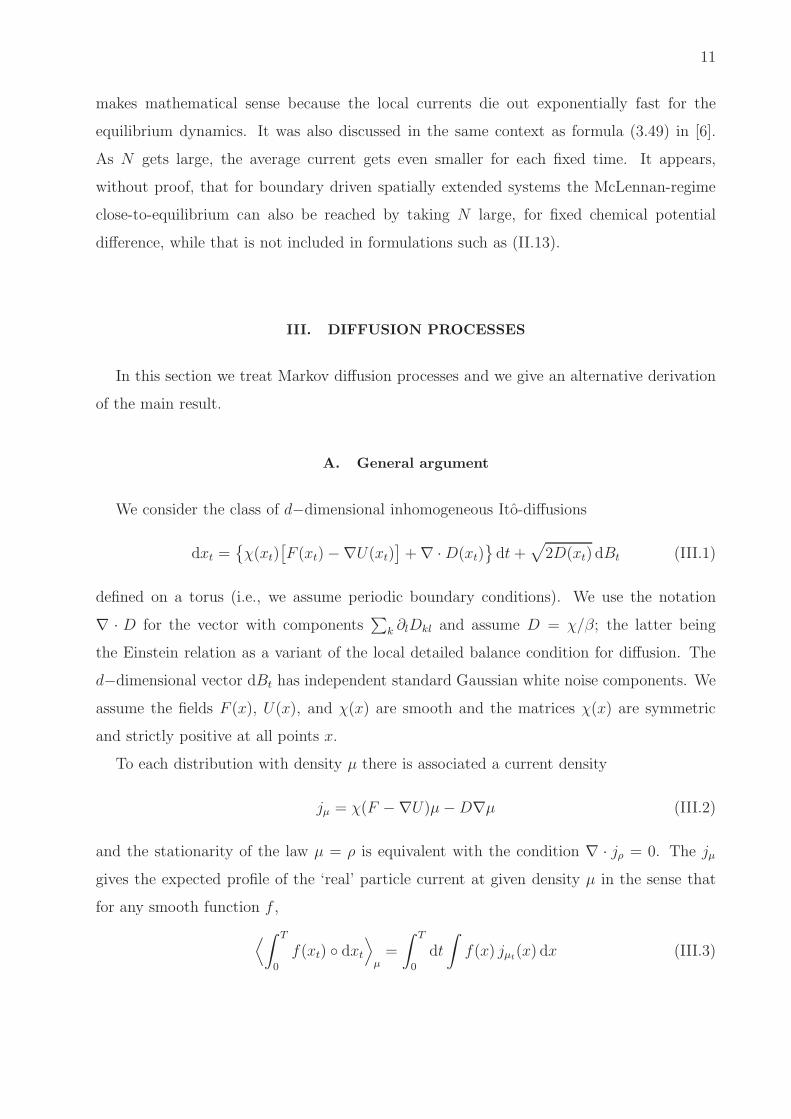
III. DIFFUSION PROCESSES

In this section we treat Markov diffusion processes and we give an alternative derivation

of the main result.

A. General argument

We consider the class of d−dimensional inhomogeneous Ito-diffusions

dxt =

χ(xt)[

F (xt) −∇U(xt)]

+ ∇ · D(xt)

dt +√

2D(xt) dBt (III.1)

defined on a torus (i.e., we assume periodic boundary conditions). We use the notation

∇ · D for the vector with components∑

k ∂lDkl and assume D = χ/β; the latter being

the Einstein relation as a variant of the local detailed balance condition for diffusion. The

d−dimensional vector dBt has independent standard Gaussian white noise components. We

assume the fields F (x), U(x), and χ(x) are smooth and the matrices χ(x) are symmetric

and strictly positive at all points x.

To each distribution with density µ there is associated a current density

jµ = χ(F −∇U)µ − D∇µ (III.2)

and the stationarity of the law µ = ρ is equivalent with the condition ∇ · jρ = 0. The jµ

gives the expected profile of the ‘real’ particle current at given density µ in the sense that

for any smooth function f ,

⟨

∫ T

0

f(xt) dxt

⟩

µ=

∫ T

0

dt

∫

f(x) jµt(x) dx (III.3)

12

The left-hand side is the average of a Stratonovich-stochastic integral under the diffusion

process started at time t = 0 from density µ. In particular, the instantaneous mean work of

the force F is then

W (µ) =

∫

F · jµ dx =

∫

wµ dx (III.4)

for

w = F · χF − χF · ∇U + ∇ · (DF ) (III.5)

In order to check the McLennan-proposal we isolate the linear order in (III.4). We take the

case F = 0, ρ0 = exp[−βU ]/Z > 0 as the equilibrium reference and we expand with small

parameter ε:

F = εF1 + . . .

w = εw1 + . . . (III.6)

ρ = ρε = ρ0(1 + εh1 + . . .)

assuming smooth behavior around ε = 0. From (III.5),

w1 = ∇ · (DF1) − χF1 · ∇U =∇ · (ρ0χF1)

βρ0

(III.7)

the linear term in the mean work performed by the force F . It turns out, as in (II.13) and

in agreement with McLennan’s proposal, that h1 is given in terms of the mean total work

performed on the particle started from x under the reference dynamics.

Theorem III.1. Suppose the process (III.1) converges exponentially fast and uniformly in

initial states to its unique stationary probability distribution with smooth density ρ around

ρ0 as in (III.6). Then,

h1(x) = −β⟨

∫ ∞

0

w1(xt) dt⟩0

x(III.8)

Proof. The current (III.2) can be rewritten in terms of the reference equilibrium density

jµ = µχ(F −∇U) − D∇µ = µχF − ρ0D∇( µ

ρ0

)

(III.9)

so that the stationarity condition ∇ · jρ = 0 implies

0 = ∇ ·[

ρ0D∇( ρ

ρ0

)

− ρχF]

= ρ0D∇ · ∇( ρ

ρ0

)

+ ρ0(∇ · D) · ∇( ρ

ρ0

)

− ρ0χ∇U · ∇( ρ

ρ0

)

−∇ · (ρχF )

= ρ0L0

( ρ

ρ0

)

−∇ · (ρχF )

(III.10)

13

with L0 the backward reference equilibrium generator. To linear order, that gives

L0h1 = βw1 (III.11)

with w1 from (III.7).

As the relaxation to equilibrium is fast enough, L0 can be inverted on the space

Ω⊥ = g :

∫

gρ0 dx = 0 (III.12)

and since w1 ∈ Ω⊥, the stationary solution must have first order

h1 = βL−10 w1 (III.13)

or

h1(x) = −β

∫ ∞

0

(

etL0w1

)

(x) dt = −β⟨

∫ ∞

0

w1(xt) dt⟩0

x(III.14)

as required.

One might be tempted to write

ρε

ρ0

(x)?= 1 − β

⟨

∫ ∞

0

w(xt) dt⟩

x+ O(ε2) (III.15)

(i.e., with the full work and possibly under the nonequilibrium measure) but this is only

formally true in the sense that the O(ε) terms on both sides are equal; however the second

term on the right-hand side generally diverges now because of its O(ε2) part. Another way

to see that is by observing that w 6∈ Ω⊥ in general, in which case L−10 w does not exist.

Still, one can proceed similarly as in the case of jump processes and add a suitable

counter-term on the right-hand side of (III.15). All that explains what is actually the

rigorous meaning of McLennan’s proposal: to correctly describe the first order correction,

one is not allowed to deal with the full transient entropy production unless the divergences

coming from the high-order corrections are removed. For safe first-order calculations one

needs to take the linear part of the entropy production functional only, as done above in

Theorem III.1.

B. Green-Kubo relations

An expression for the close-to-equilibrium stationary density obviously yields information

about the stationary current in linear response around equilibrium. That provides another

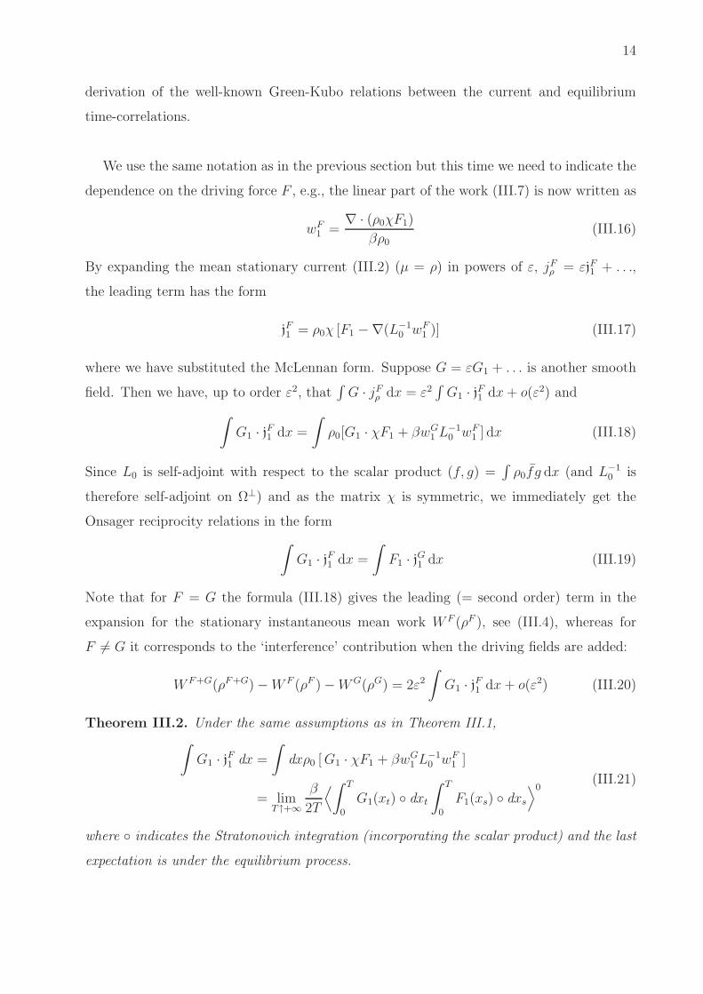
14

derivation of the well-known Green-Kubo relations between the current and equilibrium

time-correlations.

We use the same notation as in the previous section but this time we need to indicate the

dependence on the driving force F , e.g., the linear part of the work (III.7) is now written as

wF1 =

∇ · (ρ0χF1)

βρ0(III.16)

By expanding the mean stationary current (III.2) (µ = ρ) in powers of ε, jFρ = εjF1 + . . .,

the leading term has the form

jF1 = ρ0χ [F1 −∇(L−10 wF

1 )] (III.17)

where we have substituted the McLennan form. Suppose G = εG1 + . . . is another smooth

field. Then we have, up to order ε2, that∫

G · jFρ dx = ε2

∫

G1 · jF1 dx + o(ε2) and

∫

G1 · jF1 dx =

∫

ρ0[G1 · χF1 + βwG1 L−1

0 wF1 ] dx (III.18)

Since L0 is self-adjoint with respect to the scalar product (f, g) =∫

ρ0f g dx (and L−10 is

therefore self-adjoint on Ω⊥) and as the matrix χ is symmetric, we immediately get the

Onsager reciprocity relations in the form

∫

G1 · jF1 dx =

∫

F1 · jG1 dx (III.19)

Note that for F = G the formula (III.18) gives the leading (= second order) term in the

expansion for the stationary instantaneous mean work W F (ρF ), see (III.4), whereas for

F 6= G it corresponds to the ‘interference’ contribution when the driving fields are added:

W F+G(ρF+G) − W F (ρF ) − W G(ρG) = 2ε2

∫

G1 · jF1 dx + o(ε2) (III.20)

Theorem III.2. Under the same assumptions as in Theorem III.1,∫

G1 · jF1 dx =

∫

dxρ0 [ G1 · χF1 + βwG1 L−1

0 wF1 ]

= limT↑+∞

β

2T

⟨

∫ T

0

G1(xt) dxt

∫ T

0

F1(xs) dxs

⟩0(III.21)

where indicates the Stratonovich integration (incorporating the scalar product) and the last

expectation is under the equilibrium process.

15

Remark III.3. The middle term in (III.21) is what follows from applying the McLennan

formula to the mean current close-to-equilibrium. The equality (III.21) then yields the

linear response formula for the close-to-equilibrium stationary current in terms of current-

current time correlations, its right-hand side. The result can be formally summarized as

saying that

jFρ (x) =

∫

R(x, y) F (y) dy + o(ε) (III.22)

with a symmetric response function R(x, y) = R(y, x) given by

R(x, y) = limT↑+∞

β

2T

⟨

JT (x) JT (y)⟩0

(III.23)

and

JT (x) =

∫ T

0

δ(xt − x) dxt (III.24)

is the time-integrated empirical current density.

Proof. As the first equality in (III.21) is formula (III.18), we only need to prove the second

equality there.

Using the standard relation between the Stratonovich and the Ito integrals, each inte-

gration along the equilibrium process (corresponding to F = 0 in (III.1)) on the right-hand

side of (III.18) can be computed as follows:

∫ T

0

F1 dxt =

∫ T

0

F1 · dxt +

∫ T

0

∑

kl

Dkl∂F1,l

∂xkdt

=

∫ T

0

[−F1 · χ∇U + ∇ · (DF1)] dt +

∫ T

0

F1 · (2D)1/2dBt

=

∫ T

0

wF1 dt +

∫ T

0

F1 · (2D)1/2dBt

(III.25)

We must substitute (III.25) into the right-hand side of (III.21). We start with the cross

terms, one of which is

⟨

∫ T

0

wG1 dt

∫ T

0

F1 · (2D)1/2dBs

⟩

=⟨

∫ T

0

wG1 dt

∫ t

0

F1 · (2D)1/2dBs

⟩0

= −⟨

∫ T

0

wG1 dt

[

∫ T

t

F1 · (2D)1/2dBs + 2

∫ T

t

wF1 ds

]⟩0

= −2⟨

∫ T

0

wG1 dt

∫ T

t

wF1 ds

⟩0

(III.26)

16

In the second equality we have applied the time-reversal of the last equality in (III.25),

using that the Stratonovich-integral is time-antisymmetric and that the equilibrium process

is time-reversal symmetric. Analogously,⟨

∫ T

0

wF1 dt

∫ T

0

G1 · (2D)1/2dBs

⟩0

= −2⟨

∫ T

0

wF1 dt

∫ T

t

wG1 ds

⟩0

= −2⟨

∫ T

0

wG1 dt

∫ t

0

wF1 ds

⟩0(III.27)

Hence, both cross-terms together give

− 2⟨

∫ T

0

wG1 dt

∫ T

0

wF1 ds

⟩0

(III.28)

As a consequence, the correlation is then⟨

∫ T

0

G1(xt) dxt

∫ T

0

F1(xs) dxs

⟩0

= 2⟨

∫ T

0

G1 · DF1(xt) dt⟩0

−⟨

∫ T

0

wG1 (xt) dt

∫ T

0

wF1 (xs) ds

⟩0

= 2T 〈G1 · DF1〉0 −

∫ (1−α)T

αT

dt

∫ T−t

−t

ds 〈wG1 (xt) wF

1 (xs)〉0 + O(αT )

= 2T 〈G1 · DF1〉0 − (1 − 2α)T

∫ +∞

−∞

ds 〈wG1 (x0) wF

1 (xs)〉0 + O(αT ) + O(T e−καT )

for an arbitrary 0 < α < 1/2 and with κ the rate of exponential decay of the time correla-

tions. Dividing by 2T and taking the limits T ↑ +∞ and then α ↓ 0, one finally obtains

limT↑+∞

1

2T

⟨

∫ T

0

G1(xt)dxt

∫ T

0

F1(xs)dxs

⟩0

= 〈G1 ·DF1〉0−

∫ +∞

0

ds 〈wG1 esL0wF

1 〉0 (III.29)

Remark III.4. The same proof applies for jump processes. One then has the analogues wF1 =

∑

y λ0(x, y)F (x, y), F (x, y) = −F (y, x), and jF1 = γ(x, y) [F (x, y)+hF(x)−hF (y)], γ(x, y) =

ρ0(x)λ0(x, y) = γ(y, x), hF (x) = L−10 wF

1 (x), ρF (x) = ρ0(x)[1+hF (x)]. Theorem III.2 applies

equally under the condition of uniform exponential relaxation.

C. Even and odd variables: example

For models whose configurations do not transform trivially under time reversal, the above

construction requires a generalization. If the involution π, π2 = 1, is the kinematical time-

reversal on the state space, the detailed balance condition takes the generalized form

L+0 = πL0π, ρ0π = ρ0 (III.30)

17

for the adjoint L+0 in the sense

∫

f(L0g) ρ0dx =∫

(L+0 f)g ρ0dx. Typical examples are

dissipative mechanical systems, e.g. underdamped diffusion processes, with states given by

both position and momentum variables for which π turns the sign of the momentum. Models

of heat conduction are a prime example, and the close-to-equilibrium analysis would imply

Fourier’s law — if indeed the equilibrium time correlation functions can be controlled in the

Green-Kubo formula, which remains highly non-trivial, see e.g. [1, 4].

Since the McLennan form is fundamentally a consequence of the transient fluctuation

symmetry, see Section IIB, the above arguments need only minor changes. Instead of

repeating the whole derivation, we restrict ourselves to a simple example that elucidates

essential points.

We consider the model of a linear RLC-circuit with two resistors in series and one external

voltage (E); cf. Section 3.3 in [2]. The two independent free variables are the potential U

(even) over the first resistance R1 and the current I (odd) through the second resistance R2.

To have a nontrivial transient regime, an inductance L is added in series with the resistors

and also a capacitance C is connected in parallel with the first resistor. The environment is

at inverse temperature β.

The stochastic dynamics for (U, I) is given by Kirchoff’s laws combined with the Johnson-

Nyquist theory according to which resistances R1,2 immersed in a thermal environment are

source of an extra random voltage; these can be modeled as independent Brownian motions

with variance R1,2β−1 per unit time. Altogether,

CdUt =(

It −Ut

R1

)

dt + (βR1)−1/2 dB1,t

LdIt = (E − R2It − Ut) dt + (βR2)−1/2 dB2,t

(III.31)

The reference equilibrium dynamics corresponds to E = 0, for which the stationary density

reads ρ0(U, I) ∝ exp−(CU2 + LI2)/2 and the detailed balance condition (III.30) is

verified with π(U, I) = (U,−I). In the driven case, E 6= 0, and by the linearity of the

example it is again easy to compute the stationary density ρE . Instead we use this example

to illustrate and to verify the McLennan proposal (I.1).

The goal is to get ρE from physically identifying the transient entropy flux. The irre-

versible part of the dissipation here equals β times the work done by the battery as a function

18

of the trajectory ω = (Ut, It), t ∈ [0, T ]. Specifically,

STIRR

(ω) = βE

∫ T

0

It dt (III.32)

Of course, when in doubt, one can compute it also by the general algorithm as the time-

antisymmetric part of the logarithmic density of the path-measure with respect to its time-

reversal, cf. (II.5)–(II.10). By the linearity and homogeneity of the system, the source voltage

E takes over the driving parameter ε of the previous analysis and, using the notation from

there, the expected irreversible part of the dissipation is

〈STIRR

〉µ = E

∫ T

0

〈w1(It)〉0µ dt, w1 = βI (III.33)

cf. (II.9)–(II.10) or (III.4)–(III.5). It is now easy to check that the stationary density satisfies

the identities

logρE

ρ0(U, I) = −E

⟨

∫ +∞

0

w1(xt) dt⟩0,+

U,I+ O(E2)

= βE(L+0 )−1I + O(E2)

= βE( R1C

R1 + R2U +

L

R1 + R2I)

+ O(E2)

(III.34)

where the equilibrium dynamics on the first line runs according to the generator L+0 , i.e.,

backwards in time. Since it is identical to πL0π, it only generates sign changes in the

computation—that is the only point in which the previous analysis must be modified. The

result of the McLennan theory thus gives ρE correctly as the Gaussian density with the same

covariance matrix as ρ0 but with nonzero averages

〈I〉 =E

R1 + R2〈U〉 =

R1E

R1 + R2(III.35)

The point is that even in cases where computations would be more involved, the McLen-

nan formula is in terms of a physical quantity that can often be written down without the

need to go much into further details of the model.

IV. GENERALIZATION BEYOND CLOSE-TO-EQUILIBRIUM

It is natural to ask whether similar representations of the stationary distribution

remain valid also beyond close-to-equilibrium. The correction to quadratic order has been

19

systematically explored in [8, 9, 10], within the programme of steady state thermodynamics.

Here we add a general expression, (IV.2) below, from which a cumulant expansion around

equilibrium could be started in principle.

We look back at (II.5)–(II.6) that we now write as

dPµ(ω) = dP0µ(ω) e−A(ω)

where the equilibrium reference P0µ is starting from the law µ. We decompose the action A

into a time-antisymmetric and a time-symmetric part:

S = Aθ − A, T = Aθ + A

where we have abbreviated (II.7) to S. From (II.6), the time-symmetric part T is the time-

integrated excess in escape rates for jump processes. It is more generally related to the

dynamical activity in the process. We have also called it traffic in the context of dynamical

fluctuation theory, [15, 17]. We thus have

dPµ = dP0µ exp

(S − T

2

)

, dPρ0 θ = dP0 exp

(

−S + T

2

)

(IV.1)

where the second identity uses the time-reversal invariance of the equilibrium process (started

at ρ0). The integrated form of the second identity reads

〈f(ω)〉ρ0= 〈f(θω) e−

1

2(S(ω)+T (ω))〉0

with the right-most expectation over the equilibrium process. The left expectation is for the

nonequilibrium process starting in ρ0 so that, taking functions f(ω) = f(ωt) of the state

at a single time t, we get information about the approach to the nonequilibrium stationary

density. For the finite state space Ω, taking f(ω) = δxT =x, we get

Prob(xT = x) = ρεT (x) = ρ0(x) 〈e−

1

2(S+T )〉0x, x ∈ Ω (IV.2)

which is an exact formula for the nonequilibrium density at time T , no matter how far from

equilibrium, entirely in terms of the reference equilibrium dynamics starting at x. Recall

that the exponent in the average is extensive in (large) time T while also of (small) order ε

around equilibrium. Together with the normalization condition

〈e1

2(S−T )〉0µ = 1 (IV.3)

20

for all initial laws µ, as follows from the first identity in (IV.1), this can be taken as the

starting point for systematic expansions. In the first order around equilibrium, the expected

entropy flux S and the expected traffic T are identical. That explains how (II.17) and hence

McLennan’s formula follow from (IV.2). That finally is why we call (IV.2) a generalization,

still involving the irreversible entropy flux S but now also the traffic T . Note that all

expectations in (IV.2)–(IV.3) are under the equilibrium process, in contrast to a slightly

different construction suggested in [8] which only uses the variable entropy production but

with respect to the full nonequilibrium dynamics. We see that difference, equilibrium versus

nonequilibrium expectation, also when comparing (IV.2) with (II.17) where STIRR

= S:

〈e−ST

IRR 〉x = 〈e−1

2(S+T )〉0x

Yet, starting from either of the two expressions, there remains the difficulty of writing down a

general and physically meaningful expression of the stationary distribution ρ in a sufficiently

explicit way, also because of generic nonlocal aspects in the relation between potential and

stationary density, given a nonequilibrium driving, [15, 17].

Remark IV.1. The expression (IV.2) or the original McLennan formula (I.1) is perhaps

related to what is argued to follow from a maximum entropy principle, cf. [3, 5]. Remark

however that finding the correct constraints or observables for which to apply such a principle

remains highly unclear. In particular, it appears that certainly beyond linear order around

equilibrium, also the time-symmetric fluctuation sector must get involved, cf. [19].

V. CONCLUSIONS

McLennan’s formula gives a Gibbsian-like expression for the steady law close-to-

equilibrium under the condition of local detailed balance. The correction to equilibrium

involves the transient entropy flux. It was seen before in [8] how that arises from a transient

fluctuation formula. We have added mathematical precision in the order of limits (time

versus distance from equilibrium). We have shown how it relates to local equilibrium and to

the Green-Kubo relations and we have presented a generalization involving the dynamical

activity.

In our opinion it remains important to attempt a thermodynamic interpretation of also

higher order corrections to equilibrium.

21

Acknowledgments

The authors thank T. S. Komatsu, N. Nakagawa, S. Sasa, and H. Tasaki for very fruitful

discussions. K.N. acknowledges the support from the Grant Agency of the Czech Republic

(Grant no. 202/07/0404). C.M. benefits from the Belgian Interuniversity Attraction Poles

Programme P6/02.

[1] F. Bonetto, J.L. Lebowitz, and L. Rey-Bellet: Fourier’s Law: a Challenge for Theorists,

Mathematical Physics 2000, Edited by A. Fokas, A. Grigoryan, T. Kibble and B. Zegarlinsky,

Imprial College Press, 128-151 (2000).

[2] S. Bruers, C. Maes, and K. Netocny, On the validity of entropy production principles for

linear electrical circuits, J. Stat. Phys. 129, 725–740 (2007).

[3] R. Dewar, Information theory explanation of the fluctuation theorem, maximum entropy pro-

duction and self-organized criticality in non-equilibrium stationary states, J. Phys. A 36, 631

(2003).

[4] A. Kundu, A. Dhar, and O. Narayan, Green-Kubo formula for heat conduction in open sys-

tems, J. Stat. Mech., L03001 (2009).

[5] R. M. L. Evans, Rules for transition rates in nonequilibrium steady states, Phys. Rev. Lett.

92 (2004).

[6] G. L. Eyink, J. L. Lebowitz, and H. Spohn, Microscopic origin of hydrodynamic behavior:

entropy production and the steady state, In: Chaos/Xaoc. Soviet-American Perspectives on

Nonlinear Science (American Institute of Physics, New York,1990), pp. 367–391.

[7] C. Kipnis and C. Landim, Scaling Limits of Interacting Particle Systems (Springer-Verlag,

1998).

[8] T. S. Komatsu and N. Nakagawa, An expression for stationary distribution in nonequilibrium

steady states, Phys. Rev. Lett. 100, 030601 (2008).

[9] T. S. Komatsu, N. Nakagawa, S. Sasa, and H. Tasaki, Representation of nonequilibrium steady

states in large mechanical systems, J. Stat. Phys. 134, 401–423 (2009).

[10] T. S. Komatsu, N. Nakagawa, S. Sasa, and H. Tasaki, Steady State Thermodynamics for Heat

Conduction – Microscopic Derivation, Phys. Rev. Lett. 100, 230602 (2008).

22

[11] J. L. Lebowitz and P. G. Bergmann, Irreversible Gibbsian Ensembles, Annals of Physics 1, 1

(1957).

[12] J. L. Lebowitz, Stationary Nonequilibrium Gibbsian Ensembles, Physical Review 114, 1192–

1202 (1959).

[13] J. Lebowitz and H. Spohn, A Gallavotti–Cohen type symmetry in large deviation functional

for stochastic dynamics, J. Stat. Phys. 95, 333–365, 1999.

[14] C. Maes and K. Netocny, Time-reversal and entropy, J. Stat. Phys. 110, 269–310 (2003).

[15] C. Maes and K. Netocny, Canonical structure of dynamical fluctuations in mesoscopic steady

state, Europhys. Lett. 82, 30003 (2008).

[16] C. Maes, K. Netocny and B. Shergelashvili, On the nonequilibrium relation between potential

and stationary distribution for driven diffusion, Phys. Rev.E 80, 011121 (2009).

[17] C. Maes, K. Netocny and B. Wynants, Steady state statistics of driven diffusions, Physica A

387, 2675–2689 (2008).

[18] C. Maes, F. Redig and A. Van Moffaert, On the definition of entropy production, via examples,

J. Math. Phys. 41, 1528–1554 (2000).

[19] C. Maes and M. H. van Wieren, Time-symmetric fluctuations in nonequilibrium systems,

Phys. Rev. Lett. 96, 240601 (2006).

[20] J. A. McLennan Jr., Statistical mechanics of the steady state, Phys. Rev. 115, 1405–1409

(1959).

[21] J. A. McLennan Jr., Introduction to Nonequilibrium Statistical Mechanics (Prentice-Hall, En-

glewood Cliffs, NJ, 1989).

[22] S. Tasaki and T. Matsui, Fluctuation theorem, nonequilibrium steady states and McLennan-

Zubarev ensembles of a class of large quantum systems, In: Fundamental Aspects of Quantum

Physics, Tokyo (2001); QP-PQ: Quantum Probab. White Noise Anal., 17, 100 (World Sci.,

River Edge NJ 2003).