Rigorous parameterization of stable and unstable

manifolds of �xed points from Ordinary di�erential

equations with polynomial vector �eld depending on

parameters

Yann Ricaud

Department of Mathematics and Statistics

April 20, 2020

A thesis submitted in partial ful�llment of the requirements of the

degree of M.Sc. Mathematics and Statistics

c©Yann Ricaud

Abstract

Back in 1675, Ordinary di�erentials equations were already under the

scope. Throughout the years, their use has risen. Scientists began using them

with parameters to model real-life problems. Along the way, it gave birth to

stable and unstable manifolds of �xed points with a dependency on parame-

ters. Nowadays, these objects are really useful, amongst others, to spacecraft

missions. Yet, their computations are not simple and often carry errors of

approximation. To handle those matters, scientists need to develop general

rigorous methods. This thesis introduces a reliable method that, under not

too restrictive assumptions, is used to rigorously compute a local approxima-

tion of these objects. The method is based on a parameterization via power

series whose coe�cients are computed exactly from a conjugacy relation be-

tween the vector �eld of the studied system and its linearization. The method

provides control of the errors of approximation depending on the number of

coe�cients computed and the size of the domain of the parameterization.

i

Résumé

L'étude des Équations di�érentielles ordinaires remonte jusqu'en 1675. À

travers les années, elles ont été utilisées de plus en plus. Les scienti�ques ont

commencé à y ajouter des paramètres a�n de modéliser des problèmes dans

la vie courante. Ce faisant, cela a donné naissance aux variétés stables et in-

stables de points �xes avec une dépendance aux paramètres. De nos jours, ces

objets sont très utiles, entre autres, pour les missions spaciales. Pourtant, leur

calcul n'est pas simple et il est souvent accompagné d'erreurs d'approximation.

A�n de traiter ces inconvénients, les scienti�ques ont besoin de développer des

méthodes générales rigoureuses. Ce mémoire introduit une méthode �able qui,

sous des hypothèses non trop contraignantes, est utilisée pour calculer rigou-

reusement une approximation locale de ces objets. Cette méthode est basée sur

une paramétrisation en séries de puissance dont les coe�cients sont calculés

exactement à l'aide d'une relation de conjugaison entre le champ de vecteurs

du système étudié et sa linéarisation. Cette méthode fournit du contrôle sur

les erreurs d'approximation qui dépend du nombre de coe�cients calculés et

de la taille du domaine de paramétrisation.

ii

Acknowledgments

I would like to thank my supervisor, Jean-Philippe Lessard, for all the advice

he gave me throughout my thesis, I would not have been able to do it without him.

I also want to give a special thanks to my family for the support and encourage-

ments they gave me to �nish the thesis, it helped me go through.

Moreover, I would like to thank my girlfriend and her family who always encour-

aged me to advance and look for the best.

Finally, to all who supported me throughout my thesis, I thank you with the

bottom of my heart.

iii

Contents

1 Introduction 1

2 Stable and unstable manifolds 5

2.1 Topological manifolds . . . . . . . . . . . . . . . . . . . . . . . . . . . 5

2.2 Stable and unstable manifolds . . . . . . . . . . . . . . . . . . . . . . 6

2.3 Stable and unstable manifolds with parameters . . . . . . . . . . . . 18

3 Parameterization Method via power series 22

3.1 Power series . . . . . . . . . . . . . . . . . . . . . . . . . . . . . . . . 22

3.2 Operators . . . . . . . . . . . . . . . . . . . . . . . . . . . . . . . . . 26

3.3 Weighted spaces . . . . . . . . . . . . . . . . . . . . . . . . . . . . . . 27

3.4 Radii polynomials . . . . . . . . . . . . . . . . . . . . . . . . . . . . . 34

4 Practical operators 39

4.1 Fixed point operator . . . . . . . . . . . . . . . . . . . . . . . . . . . 39

4.2 Eigenvalues and eigenvectors operator . . . . . . . . . . . . . . . . . . 42

4.3 Stable and unstable manifolds coe�cients operator . . . . . . . . . . 47

5 Bounds 54

5.1 Fixed Point . . . . . . . . . . . . . . . . . . . . . . . . . . . . . . . . 56

5.2 Eigenvalues and eigenvectors . . . . . . . . . . . . . . . . . . . . . . . 60

5.3 Stable and unstable manifolds coe�cients . . . . . . . . . . . . . . . . 64

5.4 Control of the error via Radii Polynomials . . . . . . . . . . . . . . . 77

6 Applications 79

6.1 Lorenz system . . . . . . . . . . . . . . . . . . . . . . . . . . . . . . . 79

6.1.1 Fixed point (LS) . . . . . . . . . . . . . . . . . . . . . . . . . 80

6.1.2 Eigenvalues and eigenvectors (LS) . . . . . . . . . . . . . . . . 81

6.1.3 Stable and unstable manifolds coe�cients (LS) . . . . . . . . . 82

iv

6.2 Rolls and Hexagons system . . . . . . . . . . . . . . . . . . . . . . . . 86

6.2.1 Fixed point (RH) . . . . . . . . . . . . . . . . . . . . . . . . . 87

6.2.2 Eigenvalues and eigenvectors (RH) . . . . . . . . . . . . . . . 87

6.2.3 Stable and unstable manifolds coe�cients (RH) . . . . . . . . 90

7 Conclusion 93

Appendix 95

v

List of Figures

1 Example of a 1-dimensional topological manifold . . . . . . . . . . . . 6

2 Example of a non-topological manifold . . . . . . . . . . . . . . . . . 7

3 W s(0) in blue and W u(0) in red of Example 2 . . . . . . . . . . . . . 10

4 Stable and unstable manifolds at 0 � W s(0) and W u(0) respectively . 10

5 Local stable manifold W sloc

(0) (blue), local unstable manifold W uloc

(0)

(red), stable subspace Es (black) and unstable subspace Eu (magenta) 13

6 Conjugacy as a commutative diagram . . . . . . . . . . . . . . . . . . 16

7 Work done by the conjugacy . . . . . . . . . . . . . . . . . . . . . . . 17

8 Conjugacy with parameters as a commutative diagram . . . . . . . . 20

9 Lorenz local stable manifold at 0 . . . . . . . . . . . . . . . . . . . . 84

10 Lorenz global stable manifold at 0 . . . . . . . . . . . . . . . . . . . . 84

11 Lorenz local unstable manifold at 0 . . . . . . . . . . . . . . . . . . . 85

12 Lorenz global unstable manifold at 0 . . . . . . . . . . . . . . . . . . 85

vi

List of Tables

1 Lorenz Fixed Point Results . . . . . . . . . . . . . . . . . . . . . . . . 80

2 Lorenz Eigenvalues And Eigenvectors Results . . . . . . . . . . . . . 81

3 Lorenz Stable And Unstable Manifolds Results for α �xed . . . . . . 83

4 Lorenz Stable And Unstable Manifolds Results . . . . . . . . . . . . . 83

5 Rolls And Hexagons Fixed Point Results . . . . . . . . . . . . . . . . 88

6 Lorenz Eigenvalues And Eigenvectors Results . . . . . . . . . . . . . 89

7 Rolls And Hexagons Stable And Unstable Manifolds Results for α �xed 91

8 Rolls And Hexagons Stable And Unstable Manifolds Results . . . . . 91

vii

1 Introduction

The study of Ordinary di�erential equations (ODEs) dates back from 1675

(see [13]). Hence, there is a lot we know on ODEs. There are natural mathematical

objects that arise from ODEs. Some of them are �xed points, periodic orbits, stable

and unstable manifolds of �xed points, stable and unstable manifolds of periodic

orbits, etc. In particular, stable and unstable manifolds of �xed points are quite

helpful to characterize the set of initial conditions that give convergent solutions as

time goes to in�nity.

Let us focus on stable and unstable manifolds of �xed points (see Section 2).

These objects are found, among others, in biology and physics. For instance, in

predator-prey models like in [15], the study of stable manifolds enables looking at

di�erent scenarios for the convergence of solutions depending on where are located

the initial conditions and the value of the parameters. Furthermore, those models

often depends on parameters. Therefore, studying the stable manifolds with a de-

pendency on those parameters provides answers regarding the parameters values to

input in order to get desired results. Moreover, in physics, especially in space-craft

missions like in [16], the study of stable and unstable manifolds of �xed points and

periodic orbits is very useful since it optimizes the use of fuel in order for satellites

to go farther in space with less fuel. Once again, the use of parameters is useful, so

it is natural to have parameter-dependent stable and unstable manifolds.

Now, when it comes to the computation of these objects, it is often hard nay

impossible to do it by hand. Nonetheless, since the arrival of computers, the compu-

tation of these objects has become easier, although it still is hard, and has received

more attention from scientists. However, although there exists a theorem for their

existence and uniqueness, there exists no general constructive approach to compute

them. The same is true for solution of ODEs : There exists a theorem of existence

and uniqueness for the solutions (see [4]) but there exists no general constructive

approach to compute them rigorously. Nonetheless, researches have been done and

speci�c-cases methods have been developped to compute stable and unstable mani-

folds of �xed points.

In this thesis, we consider the class of ODEs given as polynomial vector �elds.

Although they are easy to write and apply to a broad variety of real-life problems,

for instance predator-prey models (see [15]) and space-craft missions (see [16]) as

mentioned above � one can recover polynomial vector �elds from the analytic ones of

1

[16] through automatic di�erentiation (see [14]) �, they are way harder to solve than

linear systems. Several methods have been developped to compute speci�c solutions

of them. Some of these methods include looking for homoclinic and heteroclinic

orbits (see [15]) and low-energy transfers (see [16]). Both of these two methods

require the computation of stable and unstable manifolds of �xed points. [15] uses

a qualitative approach that does not compute them but tell them the behavior of

the solutions � they left the computation of the stable and unstable manifolds of

their �xed points as an open question. [16] computes them by means of Newton's

method. Note that our method applies to most of the stable and unstable manifolds

of �xed points of [15]. Moreover, note that our method applies to the stable and

unstable manifolds of �xed points of [16] through automatic di�erentiation (see [14])

� the later is mandatory to convert their vector �elds to polynomial ones.

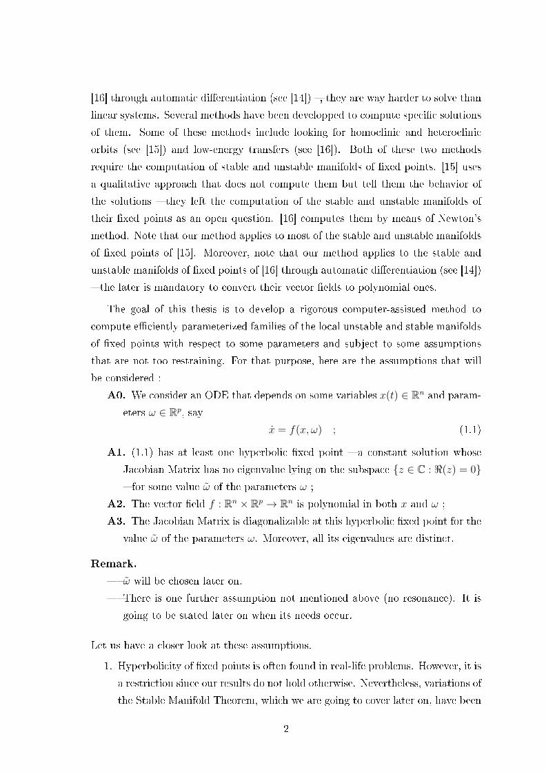
The goal of this thesis is to develop a rigorous computer-assisted method to

compute e�ciently parameterized families of the local unstable and stable manifolds

of �xed points with respect to some parameters and subject to some assumptions

that are not too restraining. For that purpose, here are the assumptions that will

be considered :

A0. We consider an ODE that depends on some variables x(t) ∈ Rn and param-

eters ω ∈ Rp, say

x = f(x, ω) ; (1.1)

A1. (1.1) has at least one hyperbolic �xed point � a constant solution whose

Jacobian Matrix has no eigenvalue lying on the subspace {z ∈ C : <(z) = 0}� for some value ω of the parameters ω ;

A2. The vector �eld f : Rn × Rp → Rn is polynomial in both x and ω ;

A3. The Jacobian Matrix is diagonalizable at this hyperbolic �xed point for the

value ω of the parameters ω. Moreover, all its eigenvalues are distinct.

Remark.

� ω will be chosen later on.

� There is one further assumption not mentioned above (no resonance). It is

going to be stated later on when its needs occur.

Let us have a closer look at these assumptions.

1. Hyperbolicity of �xed points is often found in real-life problems. However, it is

a restriction since our results do not hold otherwise. Nevertheless, variations of

the Stable Manifold Theorem, which we are going to cover later on, have been

2

studied in recent years, so one could go over our study again with a variation

of the previous theorem.

2. Many ODEs are given by polynomials. Moreover, polynomials are dense in

the set of continuous functions. Furthermore, consider that many ODEs are

piecewise continuous � x = 1xis continuous everywhere but x = 0. As seen

previously, the addition of parameter-dependency for the vector �eld actually

allows to consider many practical applications that need control to be opti-

mized � the control is done through parameter variation (again, see [15] and

[16]). Moreover, it gives rise to chaos and bifurcations in dynamical systems,

two subjects that received a lot of attention in the past 30 years.

3. The diagonalizability of the Jacobian Matrix is not too restrictive. Indeed,

diagonalization is a generic property � the set of diagonalizable matrices is

dense in the set of all matrices over the �eld C �, whence not restrictive.

Unless one chooses or makes an example with this property not being veri�ed,

the Jacobian Matrix will be diagonalizable with probability one. Moreover, the

set of matrices with distinct eigenvalues is dense in the set of all matrices over

the �eld C. Hence, even this assumption, stronger than the diagonalizability,

is not too restrictive.

As mentioned previously, the method developped in this thesis, with respect to

the above framework, allows one to compute both the stable and unstable manifolds

of �xed points of [15] and [16]. Our method uses Taylor series to parameterize the

stable and unstable manifolds of �xed points (see Section 3). Hence, our approxima-

tions are given by polynomials. Nonetheless, it is done without Newton's method.

As opposed to Newton's method, our method does not require to invert a matrix

that depends on the size of the polynomial approximation in order to get a bound

on the latter. The method developped in this thesis has already been introduced

in [2]. Nevertheless, the proofs here di�er from the ones of [2] to focus more on

the polynomial form of the vector �elds and the explicit computations of both the

approximations and the bounds. Indeed, in Section 4, we focus on the easiness

of the computations of the polynomial approximations of the stable and unstable

manifolds of �xed points, as well as on giving a proper and detailed explanation

of the computation of the bounds in Section 5. Moreover, this thesis covers a 4-

dimensional example in Section 6, thus giving more insights on the strength of the

3

method developped.

Let us brie�y mention that the work done in this thesis can be applied to other

problems that do not satisfy assumptions A1, A2 and A3. They can be studied by

going over our approach with slightly di�erent theorems that can be deduced from

ours by using other settings and going over our proofs with these in mind.

That being said, we are �rst going to talk about stable and unstable manifolds

of �xed points (Section 2) as the subject of this thesis is to compute them. Then,

we are going to talk about the method we will be using to compute them (Section

3). Finally, we will go over the practice (Sections 4 and 5) to show two examples

(Section 6) before wrapping up this thesis with a conclusion (Section 7).

4

2 Stable and unstable manifolds

2.1 Topological manifolds

To present a formal de�nition of the stable and unstable manifolds, we must

�rst go through some others. We borrow some statements of [5].

De�nition 1 (Coordinate system, chart, parameterization). LetM be a topological

space and U ⊆ M an open set. Let V ⊆ Rn be open. A homeomorphism φ : U →V , φ(u) = (x1(u), . . . , xn(u)) is called a coordinate system on U , and the functions

x1, . . . , xn the coordinate functions. The pair (U , φ) is called a chart on M. The

inverse map φ−1 is a parameterization of U .

De�nition 2 (Cover, atlas, transition maps). A cover ofM is a collection {Uα}α∈Iof open subsets of M such that this collection covers M, i.e. M =

⋃α∈I Uα. An

atlas on M is a collection of charts {Uα, φα}α∈I such that Uα covers M. The

homeomorphisms φβφ−1α : φα(Uα ∩ Uβ) → φβ(Uα ∩ Uβ) are the transition maps or

coordinate transformations.

Recall that a topological space is second countable if the topology has a countable

base, and Hausdor� if distinct points can be separated by neighbourhoods.

De�nition 3 (Topological manifold, Cr-di�erentiable manifold, smooth manifold,

analytic manifold). A second countable, Hausdor� topological space M is an n-

dimensional topological manifold if it admits an atlas {Uα, φα}, φα : Uα → Rn, n ∈ N.It is a Cr-di�erentiable manifold if all transition maps are of class Cr. It is a

smooth manifold if all transition maps are C∞ di�eomorphisms, that is, all partial

derivatives exist and are continuous. It is an analytic manifold if all transition maps

are analytic.

Notice that an atlas could contain only one chart, say {U , φ}. Thus, we would

have U = M, φ−1 would be a parameterization of the whole topological space MandM would be a smooth manifold. Nonetheless, ifM ⊆ Rm,m ∈ N, φ−1 would

not have to be di�erentiable at all. Furthermore, di�erentiability of transition maps

does not imply di�erentiability of coordinate systems or parameterizations.

Let us go over two simple examples to highlight the fact that all the coordinate

systems of an n-dimensional manifold map to Rn. Figure 1 is a 1-dimensional topo-

logical manifold. Indeed, if an atom were to move on the object, it would move

5

locally on a 1-dimensional curve, regardless of where it is. Therefore, for any point

on the object, one can always �nd a homeomorphism from some neighbourhood

of that point to the 1-dimensional open unit ball. Nevertheless, Figure 2 is not a

Figure 1 � Example of a 1-dimensional topological manifold

topological manifold. Indeed, consider any point on the object besides A and B.

An atom can only move in 1-dimension from that point. Now, consider A or B. An

atom could move in two dimensions at those points. Therefore, there is no home-

omorphism from some neighbourhood of either of them to the 1-dimensional open

unit ball. Since all the coordinate systems must map to Rn for the same n, it cannot

be a topological manifold.

2.2 Stable and unstable manifolds

To state the de�nition of a stable/unstable manifold, we must �rst talk about

�ows.

De�nition 4 (Flow). A �ow is a continuous function φ : R×Rn → Rn that satis�es

the following conditions :

1. φ(0, x) = x (∀x ∈ Rn) ;

2. φ(t1 + t2, x) = φ(t2, φ(t1, x)) (∀t1, t2 ∈ R, x ∈ Rn) .

For the sake of simplicity, we are sometimes going to write φt(x) instead of φ(t, x).

Flows are very important in ODEs since their solutions naturally give rise to

�ows. Indeed, let φ(t, x0) be the solution of some ODE with x0 as the initial condition

6

Figure 2 � Example of a non-topological manifold

at time t = 0. Then, φ(· , x0) is a �ow. Furthermore, the solution of an ODE always

exists given obvious assumptions.

Theorem 2.2.1 (The Fundamental Existence-Uniqueness Theorem). Let E be an

open subset of Rn containing x0 and assume that f ∈ C1(E). Then, there exists an

a > 0 such that the initial value problem

x = f(x)

x(0) = x0

has a unique solution x(t) on the interval [−a, a].

Proof. See [4].

The domain of the unique solution φ(t, x0)def

= x(t) of Theorem 2.2.1 can always

be extended to a maximal interval of existence and uniqueness that is open and

contains [−a, a] (see [4]). Moreover, the unique solution φ(t, x0) is always topologi-

cally conjugated �two functions f and g are topologically conjugated if there exists

a homeomorphism h such that h ◦ f = g ◦ h� to a �ow (see [4]). Henceforth, when

we refer to a �ow, we are going to refer to the solution of an ODE.

7

Recall that a �xed point x of an ODE is a point such that the �ow of the

ODE satis�es φt(x) = x (∀t ∈ R). We are now ready to state the de�nition of a

stable/unstable manifold.

De�nition 5 (Stable/unstable manifold). Let x ∈ Rn be a �xed point of some ODE

with �ow φ : R× Rn → Rn. The unstable manifold of the ODE at x is

W u(x)def

=

{x0 ∈ Rn : lim

t→−∞φt(x0) = x

}.

In the same manner, the stable manifold of the ODE at x is

W s(x)def

=

{x0 ∈ Rn : lim

t→+∞φt(x0) = x

}.

Let us go over one general example to illustrate the computation of stable and

unstable manifolds.

Example 1 (Linear ODE). Consider the ODE

x = Ax , (2.1)

where A ∈ Mn(R). Let x(0) = x0. The solution is given by x(t) = eAtx0 and 0 is

the only �xed point. Assume A is diagonalizable with real nonzero eigenvalues. Let

λ1, . . . , λk be the negative eigenvalues and λk+1, . . . , λn be the positive eigenvalues.

Let v1, . . . , vn be their associated eigenvector respectively. It is well-known that

they form a basis for Rn. Let (a1, . . . , an) ∈ Rn be the unique n-tuple such that

x0 = a1v1 + · · ·+ anvn. Then,

x(t) = a1eλ1tv1 + · · ·+ ake

λktvk︸ ︷︷ ︸xs(t)

+ ak+1eλk+1tvk+1 + · · ·+ ane

λntvn︸ ︷︷ ︸xu(t)

.

As t → ∞, xs(t) → 0. However, the limit of xu(t) as t → ∞ does not exist but for

ak+1 = · · · = an = 0. Therefore, the only way to have convergence at in�nite time is

to pick an initial condition given by a linear combination of eigenvectors associated

to negative eigenvalues and the limit will always be 0. Let

Es def

= 〈v1, . . . , vk〉 .

We have just shown that W s(0) = Es. A similar argument shows that W u(0) is

equal to Eu de�ned as

Eu def

= 〈vk+1, . . . , vn〉 .

8

The notations Es and Eu from Example 1 generalize as follows :

De�nition 6 (Linearized ODE, stable and unstable subspaces). Let x = f(x), where

f : E ⊂ Rn → Rn is continuously di�erentiable over E, be an ODE such that x0 ∈ Rn

is a �xed point. Assume Df(x0) is diagonalizable with real nonzero eigenvalues. Let

v1, . . . , vk and vk+1, . . . , vn be the eigenvectors associated to the negative and positive

eigenvalues respectively. The linearized ODE at x0 is y = Df(x0)y. We de�ne the

stable subspace Es and the unstable subspace Eu of the linearized ODE as

Es def

= y0 + 〈v1, . . . , vk〉Eu def

= y0 + 〈vk+1, . . . , vn〉.

One can verify the stable and unstable manifolds of the linearized ODE at the

�xed point 0 are always going to beW s(0) = 〈v1, . . . , vk〉 andW u(0) = 〈vk+1, . . . , vn〉.De�nition 6 will be useful later on.

Notice the stable and unstable manifolds of Example 1 are k-dimensional smooth

manifold and (n− k)-dimensional smooth manifold respectively. Moreover, both of

them are global manifolds � they are not restricted to an open neighbourhood of the

�xed point. Let us go through a quick concrete example to illustrate the dynamics

around the �xed point of a linear ODE.

Example 2. Consider the ODE (x

y

)=

(−xy

).

One can check 0 is the only �xed point and

W s(0) =

⟨(1

0

)⟩& W u(0) =

⟨(0

1

)⟩.

Figure 3 shows both the stable and unstable manifolds at 0 of Example 2. They

are both 1-dimensional smooth manifolds. Let us now go over the same example

but with non linear terms added to the ODE this time.

Example 3. Consider the ODE(x

y

)=

(−x− y2

x2 + y

)=

(−xy

)+

(−y2

x2

)︸ ︷︷ ︸G(x,y)

.

9

Figure 3 � W s(0) in blue and W u(0) in red of Example 2

The origin is a �xed point. The addition of the non linear terms G(x, y) renders the

computation of the stable and unstable manifold really hard by hand. Therefore,

the computation of the stable and unstable manifolds have been done numerically.

Figure 4a and Figure 4b show respectively the stable and unstable manifolds at the

(a) Stable manifold W s(0) (b) Unstable manifold W u(0)

Figure 4 � Stable and unstable manifolds at 0 � W s(0) and W u(0) respectively

origin. They are locally homeomorphic to the 1-dimensional open unit ball at every

point but the origin. The same argument as for Figure 2 applies to prove they are

not topological manifolds.

10

Although we cannot guarantee that stable and unstable manifolds are globally

topological manifold, the Stable and Unstable Manifold Theorem, which we will

cover later on, provides us with the existence of local stable and unstable manifold at

a �xed point that are at least C1-di�erentiable manifolds under some non-restrictive

conditions. Nevertheless, we need to make a de�nition before stating the Stable and

Unstable Manifold Theorem.

De�nition 7 (Smooth function, tangent vector, tangent space). LetM be a smooth

manifold. A smooth function onM is a real valued function fromM such that its

precomposition with a parameterization ofM is smooth wherever it is de�ned. The

set of all smooth functions onM is denoted C∞(M). Let x ∈M. A tangent vector

of M at x is a function v : C∞(M) → R such that, for every f, g ∈ C∞(M) and

a ∈ R,

1. v(f + g) = v(f) + v(g) ;

2. v(af) = av(f) ;

3. v(fg) = v(f)g(x) + f(x)v(g) .

The tangent space of M at x is the set of all tangent vectors at x and is denoted

TxM.

Though this de�nition is formal, since our stable and unstable manifolds are

going to be real manifolds, one can think of tangent vectors in the same way as in

Rn, i.e. as directional derivatives. With this in mind, we are now ready to state the

Stable and Unstable Manifold Theorem.

Theorem 2.2.2 (Stable and Unstable Manifold Theorem). Let E be an open subset

of Rn containing the origin. Consider the ODE x = f(x), where f : E → Rn. Let

f ∈ C1(E), and let φt be the �ow of the ODE. Suppose that f(0) = 0 and that

Df(0) has k eigenvalues with negative real part and n− k eigenvalues with positive

real part. Then there exists a k-dimensional di�erentiable manifold S tangent to the

stable subspace Es of the linearized ODE at 0 such that for all t ≥ 0, φt(S) ⊂ S and

for all x0 ∈ S,limt→∞

φt(x0) = 0

and there exists an n− k di�erentiable manifold U tangent to the unstable subspace

Eu of the linearized ODE at 0 such that for all t ≤ 0, φt(U) ⊂ U and for all x0 ∈ U ,

limt→−∞

φt(x0) = 0 .

11

Proof. See [4].

Remark. There exists a more general version of this theorem : If f ∈ Cr(E), then

the stable and unstable manifold are Cr-di�erentiable manifolds. Moreover, if f is

analytic over E, then the stable and unstable manifolds are analytic manifolds. This

can easily be derived directly from the proof of Perko [4].

We call local stable manifold at x, denoted W sloc

(x), the k-dimensional di�eren-

tiable manifold S whose existence is guaranteed by Theorem 2.2.2. In the same

way, we call local unstable manifold at x, denoted W uloc

(x), the n − k-dimensional

di�erentiable manifold U whose existence is guaranteed by Theorem 2.2.2.

Let us quickly come back on Example 3. Theorem 2.2.2 applied to this exam-

ple states there exists local stable and unstable manifolds that are 1-dimensional

di�erentiable manifolds tangent respectively to the stable subspace and unstable

subspace. Figure 5 shows the statement. One may notice the tangency of the man-

ifolds at the �xed point 0. Moreover, one may note that the local stable manifold

and the stable subspace share the same dimension. The same holds for the local

unstable manifold and the unstable subspace. One may verify this holds under the

same conditions of Theorem 2.2.2.

Since our vector �eld is analytic by Assumption A2 and our manifolds are real

manifolds, we would like to have analyticity of the parameterizations of our mani-

folds. However, this is not the same as having an analytic manifold since the latter

means the transition maps are analytic. Although these two matters seem unrelated,

we do have the result we strive for with the settings of Theorem 2.2.2.

Corollary 2.2.1 (Di�erentiability of Stable and Unstable Manifold Theorem). Let

us work with the same settings as Theorem 2.2.2. Both the stable and unstable

manifolds derived from Theorem 2.2.2 admit a parameterization that inherits the

same order of di�erentiability as the vector �eld.

Proof. As one goes through the proof of Theorem 2.2.2 given in [4], one can notice

the manifold considered is de�ned by only one parameterization which possess the

same order of di�erentiability as the vector �eld. We may talk about di�erentiability

of parameterizations here since the manifold considered is real.

Corollary 2.2.1 tells us that, given an hyperbolic �xed point of an ODE, there

12

Figure 5 � Local stable manifold W sloc

(0) (blue), local unstable manifold W uloc

(0)

(red), stable subspace Es (black) and unstable subspace Eu (magenta)

will always exist a parameterization of the stable manifold at the �xed point and

that it will be as di�erentiable as the vector �eld is. The same goes for the unstable

manifold at the �xed point.

Such a powerful theorem as Theorem 2.2.2 deserves a bit of history. It was �rst

introduced by Hadamard in 1901 (see [6]), though it was in 2 dimensions and the

formulation was not as concise as today. A couple of years later, in 1907, Liapunov

came up with three theorems (Théorème I, Théorème II and Théorème III, see

[7]) that better described the mathematics behind Theorem 2.2.2 as he introduced

Spectral Theory in the statements of his theorems. Many years later, in 1928,

Perron came up with a theorem of its own (Satz 11, see [8]) that introduced integral

equations as part of the proof of his theorem as well as a close formulation of his

theorem to Theorem 2.2.2. Decades later, in 1991, Perko wrote a book (see [4]) in

which Theorem 2.2.2 is proven using techniques introduced by Liapunov and Perron.

As of today, proofs of Theorem 2.2.2 refer to Perko's book. Nowadays, research has

been developped around this theorem. One may look at [1], [2] and [3] for further

readings. This thesis is a continuum of the work done in [2] as it has the same

settings as we do, including the dependency on parameters. We will come back on

that later.

13

Consider the stable manifold of a �xed point x of some ODE x = f(x) with

f : E ⊂ Rn → Rn, f ∈ C1(E,Rn) and �ow φt. Assume x is a hyperbolic �xed point,

i.e. Df(x) has no eigenvalue with zero real part. Assume all the eigenvalues are

real � we will cover the complex case later on. Assume Df(x) is diagonalizable. Let

k ∈ N be the number of negative eigenvalues. Let λ1, . . . , λk ∈ R be the negative

eigenvalues of Df(x), λk+1, . . . , λn ∈ R the positive ones and v1, . . . , vn ∈ Rn their

associated eigenvector.

Let

Λ =

λ1

. . .

λn

, A =

v1 · · · vn

.

The linearized ODE of x = f(x) at x is

y = Df(x)y

= AΛA−1y.

By performing the change of variable z = A−1y, we get the new ODE

z = Λz. (2.2)

Note that (2.2) is isomorphic to the linearized ODE because the change of variable

performed is an isomorphism. Therefore, we can work with either one of them. Let

us work with (2.2). The stable and unstable manifold of (2.2) at 0 are also called

the stable subspace, denoted Es, and unstable subspace, denoted Eu, respectively. Itwill be clear whether we use the de�nition for the stable and unstable manifolds at

0 of (2.2) or the one of Example 2. Let

Λs =

λ1

. . .

λk

, Λu =

λk+1

. . .

λn

and

As =

v1 · · · vk

, Au =

vk+1 · · · vn

.

Notice that

Λ =

(Λs 0

0 Λu

), A =

As Au

.

14

Moreover, let

Es = {zs ∈ Rn : (zs)i = 0 ∀k + 1 ≤ i ≤ n}

and

Eu = {zu ∈ Rn : (zu)i = 0 ∀1 ≤ i ≤ k}

be the stable and unstable subspace respectively of (2.2) at 0. Hence, we have

∀z ∈ Rn,∃!(zs ∈ Es, zu ∈ Eu), z = zs + zu,

i.e. Rn = Es ⊕ Eu. Thus, (2.2) is equivalent to

zs + zu =

(Λs 0

0 0

)zs +

(0 0

0 Λu

)zu .

The latter gives rise to two new ODEs that are solved separately to solve (2.2) :

z = Λsz (z ∈ Rk)

and

z = Λuz (z ∈ Rn−k) .

Note that the 0 components have been dropped in both of these ODEs. On the same

note, since the 0 components may be ignored, without loss of generality, we set

Es = Rk, Eu = Rn−k .

De�nition 8 (Open ball). We denote by Bk(a, r) ⊂ Rk the real open ball of center

a ∈ Rk, radius r > 0 and dimension k, i.e.

Bk(a, r)def

={x ∈ Rk : ‖x− a‖ < r

}.

The norm ‖· ‖ need not be speci�ed because all the norms are equivalent in spaces

of �nite dimension (see [17]). Moreover, for a general normed space (X, ‖· ‖X), we

denote by B(a, r) ⊂ X the open ball of center a ∈ X and radius r > 0, i.e.

B(a, r)def

= {x ∈ X : ‖x− a‖X < r} .

The notation Bk(a, r) will prime over B(a, r) when the normed space considered is

Rk.

By Theorem 2.2.2, the stable manifold at x is a local C1-di�erentiable manifold

of dimension k. Let P : Bk(0, r) → W sloc

(x) be a parameterization of the local

15

stable manifold at x. The existence of r > 0 is given by Theorem 2.2.2 because P

is a parameterization of a k-dimensional manifold. Furthermore, given θ ∈ Bk(0, r)

and t > 0, notice P (θ) ⊂ W sloc

(x) =⇒ φt(P (θ)) ⊂ W sloc

(x) by Theorem 2.2.2 and

eΛstθ ⊂ Bk(0, r) since Λs is the diagonal matrix of the negative eigenvalues. We

would like to derive an equation with P and its derivatives as the only unknowns.

We are going to set

P (0) = x

DP (0) = As

φt(P (θ)) = P (eΛstθ)

. (2.3)

The third equation of (2.3) is known as the conjugacy relation. Basically, we assume

that P maps orbits of the stable subspace Es of (2.2) at 0 to orbits of the local stable

manifold W sloc

(x) of x = f(x) at x. It can be seen as a commutative diagram as

illustrated in Figure 6. Figure 7 provides some insights on what the conjugacy does.

Moreover, one may notice the resemblance with the Hartman-Grobmann Theorem

(see [4]). The big di�erence there is that the Hartman-Grobmann Theorem is a

theorem on the full domain E ⊂ Rn of the vector �eld f , whereas the conjugacy

only holds on the local stable manifold W sloc

(x) at x. This assumption gives us the

Figure 6 � Conjugacy as a commutative diagram

following theorem which is the heart of our method to solve for P as we will see

later on.

16

✓

P

P

P (✓)

Rn Rn

x x

�(t, ·)<latexit sha1_base64="S8Z8xnvyFN2sI65xEoTiN1POLPw=">AAAB+HicdVDJSgNBEO1xjXHJqEcvjYkQQYaeJGS5Bb14jGAWSELo6XSSJj0L3TVCDPkSLx4U8eqnePNv7CyCij4oeLxXRVU9L5JCAyEf1tr6xubWdmInubu3f5CyD48aOowV43UWylC1PKq5FAGvgwDJW5Hi1Pckb3rjq7nfvONKizC4hUnEuz4dBmIgGAUj9exUphONRBYuOqwfwnmmZ6eJQ0rFSr6IiVMokIJbMoQUyvmKi12HLJBGK9R69nunH7LY5wEwSbVuuySC7pQqEEzyWbITax5RNqZD3jY0oD7X3eni8Bk+M0ofD0JlKgC8UL9PTKmv9cT3TKdPYaR/e3PxL68dw6DcnYogioEHbLloEEsMIZ6ngPtCcQZyYghlSphbMRtRRRmYrJImhK9P8f+kkXNc4rg3uXT1chVHAp2gU5RFLiqhKrpGNVRHDMXoAT2hZ+veerRerNdl65q1mjlGP2C9fQKbdpJn</latexit><latexit sha1_base64="S8Z8xnvyFN2sI65xEoTiN1POLPw=">AAAB+HicdVDJSgNBEO1xjXHJqEcvjYkQQYaeJGS5Bb14jGAWSELo6XSSJj0L3TVCDPkSLx4U8eqnePNv7CyCij4oeLxXRVU9L5JCAyEf1tr6xubWdmInubu3f5CyD48aOowV43UWylC1PKq5FAGvgwDJW5Hi1Pckb3rjq7nfvONKizC4hUnEuz4dBmIgGAUj9exUphONRBYuOqwfwnmmZ6eJQ0rFSr6IiVMokIJbMoQUyvmKi12HLJBGK9R69nunH7LY5wEwSbVuuySC7pQqEEzyWbITax5RNqZD3jY0oD7X3eni8Bk+M0ofD0JlKgC8UL9PTKmv9cT3TKdPYaR/e3PxL68dw6DcnYogioEHbLloEEsMIZ6ngPtCcQZyYghlSphbMRtRRRmYrJImhK9P8f+kkXNc4rg3uXT1chVHAp2gU5RFLiqhKrpGNVRHDMXoAT2hZ+veerRerNdl65q1mjlGP2C9fQKbdpJn</latexit><latexit sha1_base64="S8Z8xnvyFN2sI65xEoTiN1POLPw=">AAAB+HicdVDJSgNBEO1xjXHJqEcvjYkQQYaeJGS5Bb14jGAWSELo6XSSJj0L3TVCDPkSLx4U8eqnePNv7CyCij4oeLxXRVU9L5JCAyEf1tr6xubWdmInubu3f5CyD48aOowV43UWylC1PKq5FAGvgwDJW5Hi1Pckb3rjq7nfvONKizC4hUnEuz4dBmIgGAUj9exUphONRBYuOqwfwnmmZ6eJQ0rFSr6IiVMokIJbMoQUyvmKi12HLJBGK9R69nunH7LY5wEwSbVuuySC7pQqEEzyWbITax5RNqZD3jY0oD7X3eni8Bk+M0ofD0JlKgC8UL9PTKmv9cT3TKdPYaR/e3PxL68dw6DcnYogioEHbLloEEsMIZ6ngPtCcQZyYghlSphbMRtRRRmYrJImhK9P8f+kkXNc4rg3uXT1chVHAp2gU5RFLiqhKrpGNVRHDMXoAT2hZ+veerRerNdl65q1mjlGP2C9fQKbdpJn</latexit><latexit sha1_base64="S8Z8xnvyFN2sI65xEoTiN1POLPw=">AAAB+HicdVDJSgNBEO1xjXHJqEcvjYkQQYaeJGS5Bb14jGAWSELo6XSSJj0L3TVCDPkSLx4U8eqnePNv7CyCij4oeLxXRVU9L5JCAyEf1tr6xubWdmInubu3f5CyD48aOowV43UWylC1PKq5FAGvgwDJW5Hi1Pckb3rjq7nfvONKizC4hUnEuz4dBmIgGAUj9exUphONRBYuOqwfwnmmZ6eJQ0rFSr6IiVMokIJbMoQUyvmKi12HLJBGK9R69nunH7LY5wEwSbVuuySC7pQqEEzyWbITax5RNqZD3jY0oD7X3eni8Bk+M0ofD0JlKgC8UL9PTKmv9cT3TKdPYaR/e3PxL68dw6DcnYogioEHbLloEEsMIZ6ngPtCcQZyYghlSphbMRtRRRmYrJImhK9P8f+kkXNc4rg3uXT1chVHAp2gU5RFLiqhKrpGNVRHDMXoAT2hZ+veerRerNdl65q1mjlGP2C9fQKbdpJn</latexit>

�(t, P (✓)) = P (e⇤st✓)<latexit sha1_base64="1A+3CG8SNXD0PdqOjgycAQc3kmI=">AAACGXicbVC7SgNBFJ2NrxhfUUubwSBEkLCbRhshaGNhEcE8ILuG2cmNGTL7YOauEJb8ho2/YmOhiKVW/o2TZAtNPHDhcM69M/ceP5ZCo21/W7ml5ZXVtfx6YWNza3unuLvX1FGiODR4JCPV9pkGKUJooEAJ7VgBC3wJLX94OfFbD6C0iMJbHMXgBew+FH3BGRqpW7TdTsGNB6KMJ/WyiwNAdnx8TutluEvda/NOj3U1jmlmuV63WLIr9hR0kTgZKZEM9W7x0+1FPAkgRC6Z1h3HjtFLmULBJYwLbqIhZnzI7qFjaMgC0F46vWxMj4zSo/1ImQqRTtXfEykLtB4FvukMGA70vDcR//M6CfbPvFSEcYIQ8tlH/URSjOgkJtoTCjjKkSGMK2F2pXzAFONowiyYEJz5kxdJs1px7IpzUy3VLrI48uSAHJIyccgpqZErUicNwskjeSav5M16sl6sd+tj1pqzspl98gfW1w+Z957S</latexit><latexit sha1_base64="1A+3CG8SNXD0PdqOjgycAQc3kmI=">AAACGXicbVC7SgNBFJ2NrxhfUUubwSBEkLCbRhshaGNhEcE8ILuG2cmNGTL7YOauEJb8ho2/YmOhiKVW/o2TZAtNPHDhcM69M/ceP5ZCo21/W7ml5ZXVtfx6YWNza3unuLvX1FGiODR4JCPV9pkGKUJooEAJ7VgBC3wJLX94OfFbD6C0iMJbHMXgBew+FH3BGRqpW7TdTsGNB6KMJ/WyiwNAdnx8TutluEvda/NOj3U1jmlmuV63WLIr9hR0kTgZKZEM9W7x0+1FPAkgRC6Z1h3HjtFLmULBJYwLbqIhZnzI7qFjaMgC0F46vWxMj4zSo/1ImQqRTtXfEykLtB4FvukMGA70vDcR//M6CfbPvFSEcYIQ8tlH/URSjOgkJtoTCjjKkSGMK2F2pXzAFONowiyYEJz5kxdJs1px7IpzUy3VLrI48uSAHJIyccgpqZErUicNwskjeSav5M16sl6sd+tj1pqzspl98gfW1w+Z957S</latexit><latexit sha1_base64="1A+3CG8SNXD0PdqOjgycAQc3kmI=">AAACGXicbVC7SgNBFJ2NrxhfUUubwSBEkLCbRhshaGNhEcE8ILuG2cmNGTL7YOauEJb8ho2/YmOhiKVW/o2TZAtNPHDhcM69M/ceP5ZCo21/W7ml5ZXVtfx6YWNza3unuLvX1FGiODR4JCPV9pkGKUJooEAJ7VgBC3wJLX94OfFbD6C0iMJbHMXgBew+FH3BGRqpW7TdTsGNB6KMJ/WyiwNAdnx8TutluEvda/NOj3U1jmlmuV63WLIr9hR0kTgZKZEM9W7x0+1FPAkgRC6Z1h3HjtFLmULBJYwLbqIhZnzI7qFjaMgC0F46vWxMj4zSo/1ImQqRTtXfEykLtB4FvukMGA70vDcR//M6CfbPvFSEcYIQ8tlH/URSjOgkJtoTCjjKkSGMK2F2pXzAFONowiyYEJz5kxdJs1px7IpzUy3VLrI48uSAHJIyccgpqZErUicNwskjeSav5M16sl6sd+tj1pqzspl98gfW1w+Z957S</latexit><latexit sha1_base64="1A+3CG8SNXD0PdqOjgycAQc3kmI=">AAACGXicbVC7SgNBFJ2NrxhfUUubwSBEkLCbRhshaGNhEcE8ILuG2cmNGTL7YOauEJb8ho2/YmOhiKVW/o2TZAtNPHDhcM69M/ceP5ZCo21/W7ml5ZXVtfx6YWNza3unuLvX1FGiODR4JCPV9pkGKUJooEAJ7VgBC3wJLX94OfFbD6C0iMJbHMXgBew+FH3BGRqpW7TdTsGNB6KMJ/WyiwNAdnx8TutluEvda/NOj3U1jmlmuV63WLIr9hR0kTgZKZEM9W7x0+1FPAkgRC6Z1h3HjtFLmULBJYwLbqIhZnzI7qFjaMgC0F46vWxMj4zSo/1ImQqRTtXfEykLtB4FvukMGA70vDcR//M6CfbPvFSEcYIQ8tlH/URSjOgkJtoTCjjKkSGMK2F2pXzAFONowiyYEJz5kxdJs1px7IpzUy3VLrI48uSAHJIyccgpqZErUicNwskjeSav5M16sl6sd+tj1pqzspl98gfW1w+Z957S</latexit>

e⇤st✓<latexit sha1_base64="vuhRt3OzDybwB8Iip9XMsNG1gs8=">AAACBHicbVC7SgNBFJ2Nr7i+Vi3TDAbBKuym0TJoY2ERwTwgu4bZyU0yZPbBzF0hLCls/BUbC0Vs/Qg7/8bJo9DEAwOHc+7hzj1hKoVG1/22CmvrG5tbxW17Z3dv/8A5PGrqJFMcGjyRiWqHTIMUMTRQoIR2qoBFoYRWOLqa+q0HUFok8R2OUwgiNohFX3CGRuo6Jb9jw33u35hIj3U1TqiPQ0Bm+0HXKbsVdwa6SrwFKZMF6l3ny+8lPIsgRi6Z1h3PTTHImULBJUxsP9OQMj5iA+gYGrMIdJDPjpjQU6P0aD9R5sVIZ+rvRM4ircdRaCYjhkO97E3F/7xOhv2LIBdxmiHEfL6on0mKCZ02QntCAUc5NoRxJcxfKR8yxTia3mxTgrd88ippViueW/Fuq+Xa5aKOIimRE3JGPHJOauSa1EmDcPJInskrebOerBfr3fqYjxasReaY/IH1+QOeJJdr</latexit><latexit sha1_base64="vuhRt3OzDybwB8Iip9XMsNG1gs8=">AAACBHicbVC7SgNBFJ2Nr7i+Vi3TDAbBKuym0TJoY2ERwTwgu4bZyU0yZPbBzF0hLCls/BUbC0Vs/Qg7/8bJo9DEAwOHc+7hzj1hKoVG1/22CmvrG5tbxW17Z3dv/8A5PGrqJFMcGjyRiWqHTIMUMTRQoIR2qoBFoYRWOLqa+q0HUFok8R2OUwgiNohFX3CGRuo6Jb9jw33u35hIj3U1TqiPQ0Bm+0HXKbsVdwa6SrwFKZMF6l3ny+8lPIsgRi6Z1h3PTTHImULBJUxsP9OQMj5iA+gYGrMIdJDPjpjQU6P0aD9R5sVIZ+rvRM4ircdRaCYjhkO97E3F/7xOhv2LIBdxmiHEfL6on0mKCZ02QntCAUc5NoRxJcxfKR8yxTia3mxTgrd88ippViueW/Fuq+Xa5aKOIimRE3JGPHJOauSa1EmDcPJInskrebOerBfr3fqYjxasReaY/IH1+QOeJJdr</latexit><latexit sha1_base64="vuhRt3OzDybwB8Iip9XMsNG1gs8=">AAACBHicbVC7SgNBFJ2Nr7i+Vi3TDAbBKuym0TJoY2ERwTwgu4bZyU0yZPbBzF0hLCls/BUbC0Vs/Qg7/8bJo9DEAwOHc+7hzj1hKoVG1/22CmvrG5tbxW17Z3dv/8A5PGrqJFMcGjyRiWqHTIMUMTRQoIR2qoBFoYRWOLqa+q0HUFok8R2OUwgiNohFX3CGRuo6Jb9jw33u35hIj3U1TqiPQ0Bm+0HXKbsVdwa6SrwFKZMF6l3ny+8lPIsgRi6Z1h3PTTHImULBJUxsP9OQMj5iA+gYGrMIdJDPjpjQU6P0aD9R5sVIZ+rvRM4ircdRaCYjhkO97E3F/7xOhv2LIBdxmiHEfL6on0mKCZ02QntCAUc5NoRxJcxfKR8yxTia3mxTgrd88ippViueW/Fuq+Xa5aKOIimRE3JGPHJOauSa1EmDcPJInskrebOerBfr3fqYjxasReaY/IH1+QOeJJdr</latexit><latexit sha1_base64="vuhRt3OzDybwB8Iip9XMsNG1gs8=">AAACBHicbVC7SgNBFJ2Nr7i+Vi3TDAbBKuym0TJoY2ERwTwgu4bZyU0yZPbBzF0hLCls/BUbC0Vs/Qg7/8bJo9DEAwOHc+7hzj1hKoVG1/22CmvrG5tbxW17Z3dv/8A5PGrqJFMcGjyRiWqHTIMUMTRQoIR2qoBFoYRWOLqa+q0HUFok8R2OUwgiNohFX3CGRuo6Jb9jw33u35hIj3U1TqiPQ0Bm+0HXKbsVdwa6SrwFKZMF6l3ny+8lPIsgRi6Z1h3PTTHImULBJUxsP9OQMj5iA+gYGrMIdJDPjpjQU6P0aD9R5sVIZ+rvRM4ircdRaCYjhkO97E3F/7xOhv2LIBdxmiHEfL6on0mKCZ02QntCAUc5NoRxJcxfKR8yxTia3mxTgrd88ippViueW/Fuq+Xa5aKOIimRE3JGPHJOauSa1EmDcPJInskrebOerBfr3fqYjxasReaY/IH1+QOeJJdr</latexit>

e⇤st<latexit sha1_base64="8z7qbplblSJONvOH2KKbZDOC4Y8=">AAAB/XicdVBJSwMxGM3UrY7buNy8BIvgaciUgam3ohcPHirYBdqxZDKZNjSzkGSEOhT/ihcPinj1f3jz35gugoo+CDze+17y5QUZZ1Ih9GGUlpZXVtfK6+bG5tb2jrW715JpLghtkpSnohNgSTlLaFMxxWknExTHAaftYHQ+9du3VEiWJtdqnFE/xoOERYxgpaW+ddDrmvSm6F3qSIj7Uk3Mnt+3KshGnudUaxDZrlv1TqcEuTXXcaFjoxkqYIFG33rvhSnJY5oowrGUXQdlyi+wUIxwqq/MJc0wGeEB7Wqa4JhKv5htP4HHWglhlAp9EgVn6vdEgWMpx3GgJ2OshvK3NxX/8rq5imp+wZIsVzQh84einEOVwmkVMGSCEsXHmmAimN4VkiEWmChdmKlL+Pop/J+0qraDbOeqWqmfLeoog0NwBE6AAzxQBxegAZqAgDvwAJ7As3FvPBovxut8tGQsMvvgB4y3T+zylOM=</latexit><latexit sha1_base64="8z7qbplblSJONvOH2KKbZDOC4Y8=">AAAB/XicdVBJSwMxGM3UrY7buNy8BIvgaciUgam3ohcPHirYBdqxZDKZNjSzkGSEOhT/ihcPinj1f3jz35gugoo+CDze+17y5QUZZ1Ih9GGUlpZXVtfK6+bG5tb2jrW715JpLghtkpSnohNgSTlLaFMxxWknExTHAaftYHQ+9du3VEiWJtdqnFE/xoOERYxgpaW+ddDrmvSm6F3qSIj7Uk3Mnt+3KshGnudUaxDZrlv1TqcEuTXXcaFjoxkqYIFG33rvhSnJY5oowrGUXQdlyi+wUIxwqq/MJc0wGeEB7Wqa4JhKv5htP4HHWglhlAp9EgVn6vdEgWMpx3GgJ2OshvK3NxX/8rq5imp+wZIsVzQh84einEOVwmkVMGSCEsXHmmAimN4VkiEWmChdmKlL+Pop/J+0qraDbOeqWqmfLeoog0NwBE6AAzxQBxegAZqAgDvwAJ7As3FvPBovxut8tGQsMvvgB4y3T+zylOM=</latexit><latexit sha1_base64="8z7qbplblSJONvOH2KKbZDOC4Y8=">AAAB/XicdVBJSwMxGM3UrY7buNy8BIvgaciUgam3ohcPHirYBdqxZDKZNjSzkGSEOhT/ihcPinj1f3jz35gugoo+CDze+17y5QUZZ1Ih9GGUlpZXVtfK6+bG5tb2jrW715JpLghtkpSnohNgSTlLaFMxxWknExTHAaftYHQ+9du3VEiWJtdqnFE/xoOERYxgpaW+ddDrmvSm6F3qSIj7Uk3Mnt+3KshGnudUaxDZrlv1TqcEuTXXcaFjoxkqYIFG33rvhSnJY5oowrGUXQdlyi+wUIxwqq/MJc0wGeEB7Wqa4JhKv5htP4HHWglhlAp9EgVn6vdEgWMpx3GgJ2OshvK3NxX/8rq5imp+wZIsVzQh84einEOVwmkVMGSCEsXHmmAimN4VkiEWmChdmKlL+Pop/J+0qraDbOeqWqmfLeoog0NwBE6AAzxQBxegAZqAgDvwAJ7As3FvPBovxut8tGQsMvvgB4y3T+zylOM=</latexit><latexit sha1_base64="8z7qbplblSJONvOH2KKbZDOC4Y8=">AAAB/XicdVBJSwMxGM3UrY7buNy8BIvgaciUgam3ohcPHirYBdqxZDKZNjSzkGSEOhT/ihcPinj1f3jz35gugoo+CDze+17y5QUZZ1Ih9GGUlpZXVtfK6+bG5tb2jrW715JpLghtkpSnohNgSTlLaFMxxWknExTHAaftYHQ+9du3VEiWJtdqnFE/xoOERYxgpaW+ddDrmvSm6F3qSIj7Uk3Mnt+3KshGnudUaxDZrlv1TqcEuTXXcaFjoxkqYIFG33rvhSnJY5oowrGUXQdlyi+wUIxwqq/MJc0wGeEB7Wqa4JhKv5htP4HHWglhlAp9EgVn6vdEgWMpx3GgJ2OshvK3NxX/8rq5imp+wZIsVzQh84einEOVwmkVMGSCEsXHmmAimN4VkiEWmChdmKlL+Pop/J+0qraDbOeqWqmfLeoog0NwBE6AAzxQBxegAZqAgDvwAJ7As3FvPBovxut8tGQsMvvgB4y3T+zylOM=</latexit>

Rk<latexit sha1_base64="nrRBf32Wv4GO6OLkMds8vbfG9yg=">AAAB+3icbVC7TsMwFL0prxJeoYwsFhUSU5V0gbGChbEg2iIloXJcp7XqPGQ7iCrKr7AwgBArP8LG3+C0GaDlSJaOzrlX9/gEKWdS2fa3UVtb39jcqm+bO7t7+wfWYaMvk0wQ2iMJT8R9gCXlLKY9xRSn96mgOAo4HQTTq9IfPFIhWRLfqVlK/QiPYxYygpWWhlbDc00vwmoSBPlt8TA1PX9oNe2WPQdaJU5FmlChO7S+vFFCsojGinAspevYqfJzLBQjnBaml0maYjLFY+pqGuOISj+fZy/QqVZGKEyEfrFCc/X3Ro4jKWdRoCfLmHLZK8X/PDdT4YWfszjNFI3J4lCYcaQSVBaBRkxQovhME0wE01kRmWCBidJ1mboEZ/nLq6Tfbjl2y7lpNzuXVR11OIYTOAMHzqED19CFHhB4gmd4hTejMF6Md+NjMVozqp0j+APj8wf9p5O+</latexit><latexit sha1_base64="nrRBf32Wv4GO6OLkMds8vbfG9yg=">AAAB+3icbVC7TsMwFL0prxJeoYwsFhUSU5V0gbGChbEg2iIloXJcp7XqPGQ7iCrKr7AwgBArP8LG3+C0GaDlSJaOzrlX9/gEKWdS2fa3UVtb39jcqm+bO7t7+wfWYaMvk0wQ2iMJT8R9gCXlLKY9xRSn96mgOAo4HQTTq9IfPFIhWRLfqVlK/QiPYxYygpWWhlbDc00vwmoSBPlt8TA1PX9oNe2WPQdaJU5FmlChO7S+vFFCsojGinAspevYqfJzLBQjnBaml0maYjLFY+pqGuOISj+fZy/QqVZGKEyEfrFCc/X3Ro4jKWdRoCfLmHLZK8X/PDdT4YWfszjNFI3J4lCYcaQSVBaBRkxQovhME0wE01kRmWCBidJ1mboEZ/nLq6Tfbjl2y7lpNzuXVR11OIYTOAMHzqED19CFHhB4gmd4hTejMF6Md+NjMVozqp0j+APj8wf9p5O+</latexit><latexit sha1_base64="nrRBf32Wv4GO6OLkMds8vbfG9yg=">AAAB+3icbVC7TsMwFL0prxJeoYwsFhUSU5V0gbGChbEg2iIloXJcp7XqPGQ7iCrKr7AwgBArP8LG3+C0GaDlSJaOzrlX9/gEKWdS2fa3UVtb39jcqm+bO7t7+wfWYaMvk0wQ2iMJT8R9gCXlLKY9xRSn96mgOAo4HQTTq9IfPFIhWRLfqVlK/QiPYxYygpWWhlbDc00vwmoSBPlt8TA1PX9oNe2WPQdaJU5FmlChO7S+vFFCsojGinAspevYqfJzLBQjnBaml0maYjLFY+pqGuOISj+fZy/QqVZGKEyEfrFCc/X3Ro4jKWdRoCfLmHLZK8X/PDdT4YWfszjNFI3J4lCYcaQSVBaBRkxQovhME0wE01kRmWCBidJ1mboEZ/nLq6Tfbjl2y7lpNzuXVR11OIYTOAMHzqED19CFHhB4gmd4hTejMF6Md+NjMVozqp0j+APj8wf9p5O+</latexit><latexit sha1_base64="nrRBf32Wv4GO6OLkMds8vbfG9yg=">AAAB+3icbVC7TsMwFL0prxJeoYwsFhUSU5V0gbGChbEg2iIloXJcp7XqPGQ7iCrKr7AwgBArP8LG3+C0GaDlSJaOzrlX9/gEKWdS2fa3UVtb39jcqm+bO7t7+wfWYaMvk0wQ2iMJT8R9gCXlLKY9xRSn96mgOAo4HQTTq9IfPFIhWRLfqVlK/QiPYxYygpWWhlbDc00vwmoSBPlt8TA1PX9oNe2WPQdaJU5FmlChO7S+vFFCsojGinAspevYqfJzLBQjnBaml0maYjLFY+pqGuOISj+fZy/QqVZGKEyEfrFCc/X3Ro4jKWdRoCfLmHLZK8X/PDdT4YWfszjNFI3J4lCYcaQSVBaBRkxQovhME0wE01kRmWCBidJ1mboEZ/nLq6Tfbjl2y7lpNzuXVR11OIYTOAMHzqED19CFHhB4gmd4hTejMF6Md+NjMVozqp0j+APj8wf9p5O+</latexit> Rk

<latexit sha1_base64="nrRBf32Wv4GO6OLkMds8vbfG9yg=">AAAB+3icbVC7TsMwFL0prxJeoYwsFhUSU5V0gbGChbEg2iIloXJcp7XqPGQ7iCrKr7AwgBArP8LG3+C0GaDlSJaOzrlX9/gEKWdS2fa3UVtb39jcqm+bO7t7+wfWYaMvk0wQ2iMJT8R9gCXlLKY9xRSn96mgOAo4HQTTq9IfPFIhWRLfqVlK/QiPYxYygpWWhlbDc00vwmoSBPlt8TA1PX9oNe2WPQdaJU5FmlChO7S+vFFCsojGinAspevYqfJzLBQjnBaml0maYjLFY+pqGuOISj+fZy/QqVZGKEyEfrFCc/X3Ro4jKWdRoCfLmHLZK8X/PDdT4YWfszjNFI3J4lCYcaQSVBaBRkxQovhME0wE01kRmWCBidJ1mboEZ/nLq6Tfbjl2y7lpNzuXVR11OIYTOAMHzqED19CFHhB4gmd4hTejMF6Md+NjMVozqp0j+APj8wf9p5O+</latexit><latexit sha1_base64="nrRBf32Wv4GO6OLkMds8vbfG9yg=">AAAB+3icbVC7TsMwFL0prxJeoYwsFhUSU5V0gbGChbEg2iIloXJcp7XqPGQ7iCrKr7AwgBArP8LG3+C0GaDlSJaOzrlX9/gEKWdS2fa3UVtb39jcqm+bO7t7+wfWYaMvk0wQ2iMJT8R9gCXlLKY9xRSn96mgOAo4HQTTq9IfPFIhWRLfqVlK/QiPYxYygpWWhlbDc00vwmoSBPlt8TA1PX9oNe2WPQdaJU5FmlChO7S+vFFCsojGinAspevYqfJzLBQjnBaml0maYjLFY+pqGuOISj+fZy/QqVZGKEyEfrFCc/X3Ro4jKWdRoCfLmHLZK8X/PDdT4YWfszjNFI3J4lCYcaQSVBaBRkxQovhME0wE01kRmWCBidJ1mboEZ/nLq6Tfbjl2y7lpNzuXVR11OIYTOAMHzqED19CFHhB4gmd4hTejMF6Md+NjMVozqp0j+APj8wf9p5O+</latexit><latexit sha1_base64="nrRBf32Wv4GO6OLkMds8vbfG9yg=">AAAB+3icbVC7TsMwFL0prxJeoYwsFhUSU5V0gbGChbEg2iIloXJcp7XqPGQ7iCrKr7AwgBArP8LG3+C0GaDlSJaOzrlX9/gEKWdS2fa3UVtb39jcqm+bO7t7+wfWYaMvk0wQ2iMJT8R9gCXlLKY9xRSn96mgOAo4HQTTq9IfPFIhWRLfqVlK/QiPYxYygpWWhlbDc00vwmoSBPlt8TA1PX9oNe2WPQdaJU5FmlChO7S+vFFCsojGinAspevYqfJzLBQjnBaml0maYjLFY+pqGuOISj+fZy/QqVZGKEyEfrFCc/X3Ro4jKWdRoCfLmHLZK8X/PDdT4YWfszjNFI3J4lCYcaQSVBaBRkxQovhME0wE01kRmWCBidJ1mboEZ/nLq6Tfbjl2y7lpNzuXVR11OIYTOAMHzqED19CFHhB4gmd4hTejMF6Md+NjMVozqp0j+APj8wf9p5O+</latexit><latexit sha1_base64="nrRBf32Wv4GO6OLkMds8vbfG9yg=">AAAB+3icbVC7TsMwFL0prxJeoYwsFhUSU5V0gbGChbEg2iIloXJcp7XqPGQ7iCrKr7AwgBArP8LG3+C0GaDlSJaOzrlX9/gEKWdS2fa3UVtb39jcqm+bO7t7+wfWYaMvk0wQ2iMJT8R9gCXlLKY9xRSn96mgOAo4HQTTq9IfPFIhWRLfqVlK/QiPYxYygpWWhlbDc00vwmoSBPlt8TA1PX9oNe2WPQdaJU5FmlChO7S+vFFCsojGinAspevYqfJzLBQjnBaml0maYjLFY+pqGuOISj+fZy/QqVZGKEyEfrFCc/X3Ro4jKWdRoCfLmHLZK8X/PDdT4YWfszjNFI3J4lCYcaQSVBaBRkxQovhME0wE01kRmWCBidJ1mboEZ/nLq6Tfbjl2y7lpNzuXVR11OIYTOAMHzqED19CFHhB4gmd4hTejMF6Md+NjMVozqp0j+APj8wf9p5O+</latexit>

Figure 7 � Work done by the conjugacy

Theorem 2.2.3. (2.3) is equivalent to

P (0) = x

DP (0) = As

f(P (θ)) = DP (θ)Λsθ

. (2.4)

Proof. The �rst two conditions of (2.3) and (2.4) are shared, so only the equivalence

of the third ones needs to be proven.

=⇒ We derive both sides of the third equation of (2.3) with respect to the time

to get

f(φt(P (θ))) = DP (eΛstθ)ΛseΛstθ .

Just let t ↓ 0 to get that

f(P (θ)) = DP (θ)Λsθ ,

i.e. (2.4) holds.

⇐= Fix θ. Let

γ(t) = P (eΛstθ) .

Then, using the third equation of (2.4), we get

γ(t) = DP (eΛstθ)ΛseΛstθ

= f(P (eΛstθ))

17

= f(γ(t)) .

Therefore, by uniqueness of solutions, we have

γ(t) = φt(γ(0)) ,

which is equivalent to

P (eΛstθ) = φt(P (θ)) .

Since the argument is valid for every θ, we recover (2.3).

It is worth noticing that Theorem 2.2.3 has only P and its derivative as unknowns.

Furthermore, Theorem 2.2.3 does not depend on the parameterization P of the stable

manifold. Indeed, it holds for the parameterization P of the stable manifold at x but

it also holds for any other parameterization of the stable manifold at x, might they

exist. Moreover, Theorem 2.2.3 also holds for complex eigenvalues and eigenvectors.

We are going to tackle this matter later. Finally, P is a parameterization of the local

stable manifold at x. Hence, it is a chart, which means it de�ned in a neighbourhood

of x. Thus, Theorem 2.2.3 is a local theorem. Indeed, it does not hold globally a

priori because P is not a parameterization of the global stable manifold at x in

general.

Henceforth, we are going to refer to the third equation of (2.4) as the homological

equation. Also, Theorem 2.2.3 may be applied to Q a parameterization of the local

unstable manifold. One just needs to substitute P for Q, Λs for Λu and As for

Au. Overall, the proof remains the same, one just needs to take limits as t → −∞instead of limits as t→∞.

We can now carry over these results to the case with ODEs depending on pa-

rameters as well.

2.3 Stable and unstable manifolds with parameters

Nowadays, among others, with the enthusiasm around space missions, stable

and unstable manifolds often get to depend on parameters. One can see [12] for fur-

ther reading. Many situations have already been tackled, like when the parameters

come as Lyapunov functions (see [10]). Moreover, the study of chaos led to the study

of stable and unstable manifolds with dependency on parameters. The interested

18

reader may read [9] for deeper understanding. Furthermore, like the goal of this

thesis, methods for proving existence of stable and unstable manifolds depending on

parameters have been researched as it has been done in [11] for instance.

Fortunately, the work done in the previous subsection can be carried over to the

case where stable and unstable manifolds depend on parameters. Indeed, recall the

discussion that follows Corollary 2.2.1. We may as well add a dependency on some

parameters ω ∈ Rp for the ODE x = f(x). This would result in the ODE

∂

∂tx(t, ω) = f(x, ω) . (2.5)

Then, the subsequent objects of the discussion are all going to inherit the dependency

on ω. One can go over the details by himself, but we resume at the settings for the

conjugacy, which now become

P (0, ω) = x(ω)

DP (0, ω) = As(ω)

φt(P (θ, ω), ω) = P (eΛs(ω)tθ, ω)

. (2.6)

Fix ω ∈ Rp. Note that, by Theorem 2.2.2, the stable manifold at x(ω) is a local C1-

di�erentiable manifold of dimension k and P : Bk(0, r(ω))×Rp → W sloc

(x(ω)) is a pa-

rameterization of the local stable manifold at x(ω). The existence of r(ω) > 0 is given

by Theorem 2.2.2 because P (· , ω) is a parameterization of a k-dimensional mani-

fold. Furthermore, notice P (θ, ω) ⊂ W sloc

(x(ω)) =⇒ φt(P (θ, ω), ω) ⊂ W sloc

(x(ω))

by Theorem 2.2.2 and eΛs(ω)tθ ⊂ Bk(0, r(ω)) since Λs(ω) is the diagonal matrix of

the negative eigenvalues at ω and t > 0. Figure 8 illustrates the conjugacy for a �xed

value of ω ∈ Rp. The important matter is that the commutative diagram shown in

Figure 8 holds for �xed values of the parameters ω as it is easier to understand what

is going on if we study what occurs for a �xed value of ω and then what occurs when

we change this value. With that in mind, let us rewrite Theorem 2.2.3 to add the

parameters ω :

Theorem 2.3.1. (2.6) is equivalent to

P (0, ω) = x(ω)

DθP (0, ω) = As(ω)

f(P (θ, ω), ω) = DθP (θ, ω)Λs(ω)θ

(2.7)

for each ω ∈ Rp.

19

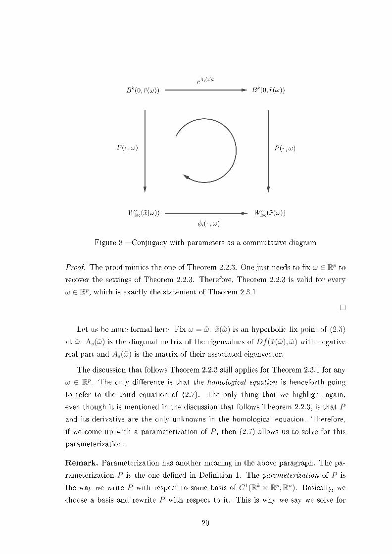
Figure 8 � Conjugacy with parameters as a commutative diagram

Proof. The proof mimics the one of Theorem 2.2.3. One just needs to �x ω ∈ Rp to

recover the settings of Theorem 2.2.3. Therefore, Theorem 2.2.3 is valid for every

ω ∈ Rp, which is exactly the statement of Theorem 2.3.1.

Let us be more formal here. Fix ω = ω. x(ω) is an hyperbolic �x point of (2.5)

at ω. Λs(ω) is the diagonal matrix of the eigenvalues of Df(x(ω), ω) with negative

real part and As(ω) is the matrix of their associated eigenvector.

The discussion that follows Theorem 2.2.3 still applies for Theorem 2.3.1 for any

ω ∈ Rp. The only di�erence is that the homological equation is henceforth going

to refer to the third equation of (2.7). The only thing that we highlight again,

even though it is mentioned in the discussion that follows Theorem 2.2.3, is that P

and its derivative are the only unknowns in the homological equation. Therefore,

if we come up with a parameterization of P , then (2.7) allows us to solve for this

parameterization.

Remark. Parameterization has another meaning in the above paragraph. The pa-

rameterization P is the one de�ned in De�nition 1. The parameterization of P is

the way we write P with respect to some basis of C1(Rk × Rp,Rn). Basically, we

choose a basis and rewrite P with respect to it. This is why we say we solve for

20

parameterized families of the local stable manifold : We parameterize P to ease

our computations of the local stable manifold. Henceforth, when we talk about a

parameterization of P , the parameterization is going to refer to the de�nition given

in this remark, whereas P will be the parameterization de�ned in De�nition 1.

We can now move on to the matter of parameterizing P .

21

3 Parameterization Method via power series

3.1 Power series

For the purpose of this thesis, we are going to study power series because

we are going to parameterize the chart P of the local stable manifold using power

series. We will see later on that doing so leads to a natural computation of local

stable manifold.

De�nition 9 (Multi-index). Let α ∈ Nd. Then, we de�ne |α|, the order of α, by

|α| def

= α1 + · · ·+ αd .

Therefore, the set {|α| = n} for n ∈ N is the set

{|α| = n} def

= {α ∈ Nd : |α| = n} .

Henceforth, for the sake of simplicity, we are just going to write |α| = n instead of

{|α| = n}. Furthermore, for α, β ∈ Nd, we de�ne the relation of order ≤ by

α ≤ β ⇐⇒ αi ≤ βi (∀1 ≤ i ≤ d)

and, similarly, the relation of strict order < by

α < β ⇐⇒(αi ≤ βi (∀1 ≤ i ≤ d) & ∃i ∈ {1, . . . , d}, αi < βi

).

The relations ≥ and > are de�ned in a similar manner, just substitute ≤ for ≥ and

< for > in this de�nition. Moreover, notice that

|α1 + α2| = |α1|+ |α2| .

Finally, for x ∈ Rd, we de�ne

xαdef

= xα11 · · ·xαdd .

It will be clear whether we use |· | to denote the absolute values or the multi-

index notation. Indeed, given that we pick α ∈ Nd, it would not make any sense to

speak of the absolute value of α since α is already nonnegative in every component.

Therefore, the reader can assume |· | is always going to denote the multi-index no-

tation whenever its argument is in Nd for some d > 0 and is always going to denote

the absolute values whenever its argument is in Rn for some n > 0.

We can now talk about power series.

22

De�nition 10 (Power series). A power series for g ∈ Cω(Rn,Rn) � g ∈ Cω(Rn,Rn)

means g : Rn → Rn is analytic in every one of its components � at x ∈ Rn is a series

such that

g(x) =∑|α|≥0

aα(x− x)α ,

where α ∈ Nn and aα ∈ Rn def

= (aα1 , . . . , aαn) ∈ Rn (∀α).

Remark. The coe�cient of g at α = (0, . . . , 0) ∈ Nn is henceforth going to be

denoted by a0. We are going to refer to the coe�cient aα as the α-th coe�cient.

Basically, a power series for g ∈ Cω(Rn,Rn) at x ∈ Rn is a Taylor series for g

at x whose existence is guaranteed by the fact that g is analytic. The radius of

convergence R of the power series for g at x is a nonnegative real number such that

the power series converges for every x ∈ B(x, R).

Having de�ned power series, it is natural to talk about recurrence relations.

De�nition 11 (Recurrence relation). Let a = (aα)|α|≥0 be a sequence of real num-

bers with α ∈ Nd (d > 0). A recurrence relation onto a is a relation R such that

aα = R(aα−) (∀|α| ≥ 1) ,

where aα− = (aα∗)α∗<α. In other words, a recurrence relation onto a is a relation

R that gives every member of the sequence, besides the �rst one, as a computation

depending on members of lesser order only.

In the case of power series, if one has an equation F (x, ω) = 0, where F ∈Cω(Rm ×Rp,Rn) and ω ∈ Rp are parameters, then one can look for a solution x(ω)

given as power series, say x(ω) =∑|β|≥0 bβω

β. With these settings and b0 given,

the coe�cients b = (bβ)|β|≥0 of the power series of x(ω) are going to be given by a

recurrence relation. This remains true when F also depends on derivatives of x(ω).

Before going over an example, let us introduce further notation for the sake of

simplicity. Let P : Rm → Rn and Q : Rm → Rn be power series given by

P (x) =∑|α|≥0

aαxα , Q(x) =

∑|α|≥0

bαxα ,

where α ∈ Rm and aα, bα ∈ Rn (∀α). Recall that the sum of two power series is

P (x) +Q(x) =∑|α|≥0

(aα + bα)xα .

Before recalling the product of two power series, let us make a useful de�nition :

23

De�nition 12 (Cauchy product). Let a = (aα)α∈Nd and b = (bα)α∈Nd be sequences

of real numbers. The Cauchy product of a and b, denoted a∗b, is de�ned component-

wise by

(a ∗ b)α def

=∑

α1+α2 = α

α1, α2 ∈ Nd

aα1bα2 .

Moreover, for β ∈ Nl and a1 = ((a1)α)α∈Nd , . . . , al = ((al)α)α∈Nd sequences of real

numbers, we de�ne

aβ11 ∗ · · · ∗ aβlldef

= a1 ∗ · · · ∗ a1︸ ︷︷ ︸β1 times

∗ · · · ∗ al ∗ · · · ∗ al︸ ︷︷ ︸βl times

.

Notice that, for η ∈ R and a = (aα)α∈Nd , b = (bα)α∈Nd , c = (cα)α∈Nd sequences of

real numbers, we have

a∗b = b∗a & η· (a∗b) = (η· a)∗b = a∗(η· b) & a∗b∗c def

= (a∗b)∗c = a∗(b∗c) ,

so there is no ambiguity in De�nition 12. Moreover, one can check that

(a+ b) ∗ c = (a ∗ c) + (b ∗ c) .

With De�nition 12 in mind, notice the product of two power series is given by

P (x)·Q(x) =∑|α|≥0

(a ∗ b)αxα .

We can now make an example to illustrate how one can retrieve recurrence relations.

Example 4. Consider the Cauchy problem{x = x(x− 1)

x(0) = x0

,

where x depends on the time t and x0 ∈ R. Suppose x is given by x(t) =∑

β≥0 bβtβ,

where β ∈ R and bβ ∈ R (∀β). Then, by substituting the power series of x into the

equation, gathering the coe�cients of the same power of t and rearranging them,

one can check we get

β· bβ = (b ∗ b)β−1 − bβ−1 (∀β ≥ 1) .

Hence, we get the relation

bβ = R(bβ−)def

=1

β((b ∗ b)β−1 − bβ−1) (∀β ≥ 1) .

According to De�nition 11, R(bβ−) is a recurrence relation.

24

Let us do another example with some parameters in it this time to see how one

can retrieve recurrence relations when parameters are involved.

Example 5. Consider the equation(−x2

1 + x2 + ω2

x22 + x1ω

)= 0 subject to x(0) =

(3

4

),

where x depends on ω. Suppose x is given by the power series x(ω) =∑|β|≥0 bβω

β,

where β ∈ N and bβ ∈ R2 (∀β). Then, by substituting the power series of x into the

equation, gathering the coe�cients of the same power of ω and rearranging them,

one can check we get(−2(b1)0 1

0 2(b2)0

)︸ ︷︷ ︸

B

·(

(b1)β

(b2)β

)=

((b1∗b1)β − δβ,2

−(b2∗b2)β − (b1)β−1

)(∀β ≥ 1) ,

where δi,jdef

=

1 , if i = j

0 otherwise(i, j ∈ N) is the Kronecker delta, (b1∗b1)β

def

= (b1 ∗

b1)β − 2(b1)0(b1)β and (b2∗b2)βdef

= (b2 ∗ b2)β − 2(b2)0(b2)β. Notice both (b1∗b1)β and

(b2∗b2)β do not depend on bβ. Moreover, notice b0 = (3, 4). Hence, B is invertible

and we get the relation((b1)β

(b2)β

)= R(bβ−)

def

= B−1

((b1∗b1)β − δβ,2

−(b2∗b2)β − (b1)β−1

)(∀β ≥ 1) .

According to De�nition 11, R(bβ−) is a recurrence relation.

As we have seen in Examples 4 and 5, when we have an ODE with a polynomial

vector �eld, we can solve for analytic solutions. The thing to notice here is that

retrieving the recurrence relation is by far not a hard task and not computational-

heavy. Thus, it is an e�cient method to �nd solutions of ODE. However, we need

the invertibility of the matrix B. This matter is going to be discussed thoroughly

in Section 4 when we talk explicitly about our computations.

Even though we are not going to compute solutions of ODEs, our computations

are going to resemble the ones for an analytic solution of an ODE with a polynomial

vector �eld. We are going to use power series for all of them. We are going to

discuss the existence and uniqueness of our computations as well. Nevertheless,

without properly speaking of existence, one could argue that it is natural to look

25

for power series solutions of polynomial equations � we mean by that every member

of these equations is a polynomial. Nonetheless, we are going to develop a rigorous

computer-assisted proof for our computations that will ensure their existence and

uniqueness afterward (see Subsection 3.4).

Let us now move to the next subsection and talk about the kind of operator that

will be considered in Section 4 for our computations.

3.2 Operators

Recall Equations 2.7. Recall our goal is to compute a parameterization of the

local stable manifoldW sloc

(x(ω)) at the �xed point x(ω) depending on the parameters

ω � without loss of generality, we consider the local stable manifold instead of the

local unstable manifold because the computations are the same, only the inputs

di�er slightly. We are going to parameterize P using power series. The �rst two

equations of (2.7) are the initial conditions for the coe�cients of the power series of

P while the third is the homological equation.

Suppose the �xed point, eigenvalues, eigenvectors and P are given by power

series. Equations for computing �xed points, eigenvalues and eigenvectors are well-

known. Moreover, the homological equation gives us a way to compute P given a

parameterization of the latter. Hence, as seen in Example 5 and discussed thoroughly

in Section 4, we will have recurrence relations onto the coe�cients of those power

series using the aforementioned equations � they will be covered explicitly in Section

4. Nevertheless, since we can only compute �nitely many coe�cients, we want to

compute enough so we have "good" approximations � we will see later what we mean

by a good approximation � of these power series but not too much in order to keep

control on the error associated to the computer itself.

Consider any of the power series mentioned above. Let z = (zδ)|δ|≥0 be its

coe�cients. Assume we have already computed all its coe�cients up to orderN−1 >

0, i.e. all its coe�cients zδ such that |δ| ≤ N − 1 � we will see in the next section

there is a way to choose N . Recall De�nition 11. Assume we have the recurrence

relation

zδ = R(zδ−)

onto the coe�cients. Let zNdef

= {zδ : |δ| ≤ N − 1} be the set of the coe�cients of

order less than N , i.e. those that have already been computed. Let z be de�ned

26

component-wise by

zδdef

=

zδ , if |δ| ≤ N − 1

0 , otherwise.

z is the coe�cients of the approximation of the power series, i.e. those of zN and 0s

for all the coe�cients at indices |δ| ≥ N . The operator T we solve to get existence

and uniqueness of the "true" power series � the power series with all the coe�cients,

not only �nitely many computed � is de�ned component-wise by

(T (u))δdef

=

0 , if zδ ∈ zN

R((z + u)δ−

), otherwise

. (3.1)

The spaces in which the domain and the image of T lie are going to be explicited in

Section 4. Basically, we want to check that the approximation of the power series

we computed is close enough to the true power series. Since the coe�cients zN

we have already computed are the exact coe�cients, we just need to have a bound

on the tail of the power series for which we can guarantee the smallness. Hence,

for now, try to think of the operator T as the distance coe�cient-wise between

the approximation of the power series and the true power series. Since the distance

coe�cient-wise between the computed coe�cients of the approximation of the power

series � the coe�cients z � and the corresponding coe�cients of the true power series

� the coe�cients z � is 0, T takes the value of 0 at the indices referring to them

� the indices δ such that |δ| ≤ N − 1. For the rest of the indices, the distance

component-wise is just the value of the coe�cient of the true power series for each

index. Thus, the value of T at those indices is the value of the recurrence relation

at these. Since we cannot evaluate the recurrence relation at the coe�cients of the

true power series, we feed T the coe�cients of the approximation of the power series

plus a small variation u. The purpose of the operator T and the number N is to

prove z is a good enough approximation of the coe�cients of the true power series.

Now is the time to de�ne the spaces on which the operator T is going to act so

we can speak afterward of what a good enough approximation is to us.

3.3 Weighted spaces

Whenever one works with power series, there is always the lurking question

of convergence, namely how big the radius of convergence is. Weighted spaces are

natural spaces to work with power series because the radius of convergence can be

27

seen as a weight added on a functional space. We are going to consider certain

weighted spaces that �t the use of operators de�ned as in (3.1). Though they can

be de�ned for complex sequences, for the sake of simplicity, they are de�ned for

real sequences � we will discuss in Section 4 the case of complex sequences when it

occurs.

De�nition 13 (`1ν spaces). Let d, p, n,N ∈ N. Let ν ∈ Rd

+ and µ ∈ Rp+ � Rd

+ is the

subset of Rd whose elements have positive components. We de�ne the `1ν spaces as

`1ν

def

=

a = (aα)α∈Nd ⊂ Rn :∑|α|≥0

|aα|να <∞

`1ν,µ

def

=

a = (aα,β)(α,β)∈Nd+p ⊂ Rn :∑|β|≥0

∑|α|≥0

|aα,β|ναµβ <∞

`1,Nν

def

={a ∈ `1

ν : aα = 0 (∀|α| < N)}

`1,Nν,µ

def

={a ∈ `1

ν,µ : aα,β = 0 (∀|α| < N)}

.

For M ∈ N, we can consider the product of each of these `1ν spaces with itself M

times, i.e. (`1ν)M,(`1ν,µ

)M,(`1,Nν

)Mand

(`1,Nν,µ

)Mrespectively.

Remark. Let X be any of the spaces of De�nition 13. Then, for any a = (aδ)δ∈Nl ∈X (l > 0), we have |a| ∈ X, where |a| is de�ned component-wise by

(|a|)δ

def

= |aδ|.

If one sees the sequences involved in the de�nition of those spaces as coe�cients

of some power series, then the condition for these sequences to belong to those spaces

is just the convergence of their power series. The next de�nition sets the condition

to be a norm.

De�nition 14 (Norms on `1ν spaces). Recall De�nition 13. Then,

‖a‖1,νdef

=∑|α|≥0

|aα|να (a ∈ `1ν)

‖a‖1,(ν,µ)def

=∑|β|≥0

∑|α|≥0

|aα|ναµβ (a ∈ `1ν,µ)

‖a‖1,ν,Ndef

=∑|α|≥N

|aα|να (a ∈ `1,Nν )

‖a‖1,(ν,µ),Ndef

=∑|β|≥0

∑|α|≥N

|aα|ναµβ (a ∈ `1,Nν,µ )

.

28

Furthermore,

‖a‖(M)1,ν

def

= max {‖a1‖1,ν , . . . , ‖aM‖1,ν}(a ∈ (`1

ν)M)

‖a‖(M)1,(ν,µ)

def

= max{‖a1‖1,(ν,µ), . . . , ‖aM‖1,(ν,µ)

} (a ∈

(`1ν,µ

)M)‖a‖(M)

1,ν,Ndef

= max {‖a1‖1,ν,N , . . . , ‖aM‖1,ν,N}(a ∈

(`1,Nν

)M)‖a‖(M)

1,(ν,µ),N

def

= max{‖a1‖1,(ν,µ),N , . . . , ‖aM‖1,(ν,µ),N

} (a ∈

(`1,Nν,µ

)M).

One can verify that ‖· ‖1,ν : `1ν → R, ‖· ‖1,(ν,µ) : `1

ν,µ → R, ‖· ‖1,ν,N : `1,Nν → R,

‖· ‖1,(ν,µ),N : `1,Nν,µ → R, ‖· ‖(M)

1,ν : (`1ν)M → R, ‖· ‖(M)

1,(ν,µ) :(`1ν,µ

)M → R, ‖· ‖(M)1,ν,N :(

`1,Nν

)M → R and ‖· ‖(M)1,(ν,µ),N :

(`1,Nν,µ

)M → R are norms on their respective space of

De�nition 13.

The purpose of the norms of De�nition 14 is they de�ne a Banach space � a

complete metric space with a norm � on their respective space. One can prove this

using the fact R is a complete space. As we will see in the next subsection, our

method to ensure that our computations are good enough approximations requires

Banach spaces to work on.

Recall a Banach algebra is a Banach space (B, ‖· ‖B) together with an algebra

∗ : B ×B → B such that ‖a ∗ b‖B ≤ ‖a‖B‖b‖B for all a, b ∈ B.

Theorem 3.3.1. Recall De�nition 12. Let ν ∈ Rd+, µ ∈ Rp

+ and N be a positive

integer. Then, (X, ‖· ‖X) together with the Cauchy product ∗ is a Banach algebra �

(X, ‖· ‖X) is any Banach space of De�nition 13 coupled with its norm of De�nition

14.

Proof. Let a, b ∈ `1ν . We already know the Cauchy product is an algebra by Subsec-

tion 3.1. Thus, we only need to verify that ‖a ∗ b‖1,ν ≤ ‖a‖1,ν‖b‖1,ν . Indeed, it will

also prove a ∗ b ∈ `1ν since ‖a‖1,ν , ‖b‖1,ν <∞ by assumption. Observe that

m∑|α|=0

|(a ∗ b)α|να =m∑|α|=0

∣∣∣∣∣∣∣∑

α1+α2=α

α1,α2∈Nd

aα1bα2

∣∣∣∣∣∣∣ να

≤m∑|α|=0

∑α1+α2=α

α1,α2∈Nd

∣∣aα1bα2

∣∣ να

≤

m∑|α|=0

|aα|να m∑

|α|=0

|bα|να .

29

Hence,

‖a ∗ b‖1,ν = limm→∞

m∑|α|=0

|(a ∗ b)α|να

≤ limm→∞

m∑|α|=0

|aα|να m∑

|α|=0

|bα|να

= ‖a‖1,ν‖b‖1,ν

<∞

where the strict inequality comes from the fact both a and b lie in `1ν .

The same argument can be applied to show ∗ is also a Banach algebra over the

other Banach spaces. Indeed, notice `1,Nν is a subspace of `1

ν , `1ν,µ is exactly `1

ν with

ν = (ν, µ) and `1,Nν,µ is a subspace of `1

ν,µ, so the argument works for each of them.

Finally, knowing ∗ is a Banach algebra over each of the previous four spaces, one

can easily prove ∗ is also a Banach algebra over the �nite product of any of them

with itself.

Theorem 3.3.1 is really handy because the Cauchy product arises naturally in

product of power series and it gives us a bound on the coe�cients of those prod-

ucts. Notice Theorem 3.3.1 also applies to the hat Cauchy product of De�nition 15.

Nonetheless, for the later, we would like to get a better bound on the coe�cients of

the product of power series than the bound given by the Banach algebra. To this

end, we must �rst make a proposition.

Proposition 3.3.1. Recall De�nition 13. Let a ∈ `1ν and b ∈ `1,N

ν . Then, a∗b ∈ `1,Nν

and

‖a ∗ b‖1,ν,N ≤ ‖a‖1,ν‖b‖1,ν,N .

Proof. First of all, notice that

(a ∗ b)α =∑

α1+α2=α

aα1bα2 = 0 ∀|α| < N

since bα = 0 for all |α| < N . Now, showing the estimate on the `1,Nν -norm of a ∗ b

will also prove that the latter belongs to `1,Nν . Since `1,N

ν ⊂ `1ν , both b and a ∗ b

belong to `1ν . By Theorem 3.3.1, we have

‖a ∗ b‖1,ν ≤ ‖a‖1,ν‖b‖1,ν .

30

Therefore, since ‖b‖1,ν = ‖b‖1,ν,N and ‖a ∗ b‖1,ν = ‖a ∗ b‖1,ν,N , we have

‖a ∗ b‖1,ν,N ≤ ‖a‖1,ν‖b‖1,ν,N .

Proposition 3.3.1 also works for a ∈ `1ν,µ and b ∈ `1,N

ν,µ . As mentioned above, this

proposition is a tool to prove the next theorem. Nonetheless, we also need a lemma

to prove it, lemma that requires to make a de�nition �rst.

De�nition 15 (Hat Cauchy product). Recall De�nition 12. Let a = (aα)α∈Nd and

b = (bα)α∈Nd be sequences of real numbers. The hat Cauchy product of a and b,

denoted a ∗ b, is de�ned component-wise by

(a ∗ b)α def

=

0 , if α = 0

(a ∗ b)α − aαb0 − a0bα , otherwise.

Moreover, for β ∈ Nl and a1 = ((a1)α)α∈Nd , . . . , al = ((al)α)α∈Nd sequences of real

numbers, we de�ne aβ11 ∗ · · · ∗ aβll component-wise by

(aβ11 ∗ · · · ∗ aβll )αdef

=

0 , if α = 0

(aβ11 ∗ · · · ∗ aβll )α − β1(a1)α(a1)β1−10 (a2)β20 . . . (al−1)

βl−1

0 (al)βl0

− · · · − βl(a1)β10 (a2)β20 . . . (al−1)βl−1

0 (al)βl−10 (al)α

, otherwise.

For the sake of simplicity, we are henceforth going to write a∗b instead of a ∗ bwhenever the hat Cauchy product only involves two sequences of real numbers.

Remark.

� One may notice the hat Cauchy product is not an associative operation in

the sense that, in general, for a, b, c sequences of real numbers,

a ∗ b ∗ c 6= (a∗b)∗c 6= a∗(b∗c) .

� De�nition 15 naturally arises with the use of recurrence relation. For instance,

recall Example 5. The hat Cauchy product had already been introduced

there.

With De�nition 15 in hand, we can state the lemma needed to prove the next

theorem.

31

Lemma 3.3.1. Recall De�nition 15. Let a1, . . . , aq ∈ `1ν and M > 0. Then,

M∑|α|=0

|(a1 ∗ · · · ∗ aq)α|να ≤M∑|α|=0

(|a1| ∗ · · · ∗ |aq |)ανα .

Proof. Notice

M∑|α|=0

|(a1 ∗ · · · ∗ aq)ανα| =M∑|α|=0

∣∣∣∣∣∣∣∣∣∑

α1+···+αq=α|α1|,...,|αq |≥0α1,...,αq 6=α

aα1· . . . · aαq

∣∣∣∣∣∣∣∣∣ να

≤M∑|α|=0

∑α1+···+αq=α|α1|,...,|αq |≥0α1,...,αq 6=α

|aα1 |· . . . · |aαq |

να

=M∑|α|=0

(|a1| ∗ · · · ∗ |aq |)ανα .

With Proposition 3.3.1 and Lemma 3.3.1 in hand, we can now state a theorem

that strengthens the bound of the Banach algebra when the hat Cauchy product is

used.

Theorem 3.3.2. Recall De�nition 15. Let r > 0. If a1, a2, . . . , aq−1 ∈ `1ν and

aq ∈ `1,Nν with ‖aq‖1,ν,N = r, then a1 ∗ a2 ∗ · · · ∗ aq ∈ `1,N

ν and

‖a1 ∗ a2 ∗ · · · ∗ aq‖1,ν,N ≤ ‖a1‖1,ν‖a2‖1,ν · · · ‖aq−1‖1,ν · r − |(a1)0|· |(a2)0| · · · |(aq−1)0|· r .

Proof. First of all, note that

(a1 ∗ a2 ∗ · · · ∗ aq)α =∑

α1+α2+···+αq=αα1,α2,...,αq 6=α

(a1)α1(a2)α2 · · · (aq)αq = 0 (∀|α| < N)

since |αq| ≤ |α| < N and (aq)αq = 0 for all |αq| < N . Now, showing the estimate on

the `1,Nν -norm of a1 ∗ a2 ∗ · · · ∗ aq will also prove that the latter belongs to `1,N

ν . For

M > N , by lemma 3.3.1, notice we have

M∑|α|=N

|(a1 ∗ a2 ∗ · · · ∗ aq)α|να ≤M∑|α|=N

(|a1| ∗ |a2| ∗ · · · ∗ |aq |)ανα

32

=M∑|α|=N

((|a1| ∗ |a2| ∗ · · · ∗ |aq|)α − |(a1)0|· |(a2)0| · · · |(aq−1)0|· |(aq)α|) να .

Hence, taking the limit as M →∞ of the above, we get

‖a1 ∗ a2 ∗ · · · ∗ aq‖1,ν,N = limM→∞

M∑|α|=N

|(a1 ∗ a2 ∗ · · · ∗ aq)α|να

≤ limM→∞

M∑|α|=N

((|a1| ∗ |a2| ∗ · · · ∗ |aq|)α − |(a1)0|· |(a2)0| · · · |(aq−1)0|· |(aq)α|) να

= ‖|a1| ∗ |a2| ∗ · · · ∗ |aq|‖1,ν,N − |(a1)0|· |(a2)0| · · · |(aq−1)0|· ‖|aq|‖1,ν,N .

By proposition 3.3.1, we get

‖a1 ∗ a2 ∗ · · · ∗ aq‖1,ν,N ≤ ‖|a1|‖1,ν‖|a2|‖1,ν · · · ‖|aq−1|‖1,ν‖|aq|‖1,ν,N − |(a1)0|· |(a2)0| · · · |(aq−1)0|· ‖|aq|‖1,ν,N

= ‖a1‖1,ν‖a2‖1,ν · · · ‖aq−1‖1,ν‖aq‖1,ν,N − |(a1)0|· |(a2)0| · · · |(aq−1)0|· ‖aq‖1,ν,N

= ‖a1‖1,ν‖a2‖1,ν · · · ‖aq−1‖1,ν · r − |(a1)0|· |(a2)0| · · · |(aq−1)0|· r .

The last equality uses the assumption ‖aq‖1,ν,N = r.

One can go over the same argument to show Theorem 3.3.2 also holds for

a1, a2, . . . , aq−1 ∈ `1ν,µ and aq ∈ `1,N

ν,µ with ‖aq‖1,(ν,µ),N = r. This theorem is going to

be handy later on when we go over some examples.

De�nition 16. Recall Theorem 3.3.2. For the sake of simplicity, we de�ne

‖a1‖1,ν‖a2‖1,ν · · · ‖aq−1‖1,νdef

= ‖a1‖1,ν‖a2‖1,ν · · · ‖aq−1‖1,ν − |(a1)0(a2)0 · · · (aq−1)0|

for a1, a2, . . . , aq−1 ∈ `1ν and aq ∈ `1,N

ν with ‖aq‖1,ν,N = 1. In the same way, we also

de�ne

‖a1‖1,(ν,µ)‖a2‖1,(ν,µ) · · · ‖aq−1‖1,(ν,µ)def

= ‖a1‖1,(ν,µ)‖a2‖1,(ν,µ) · · · ‖aq−1‖1,(ν,µ)−|(a1)0,0(a2)0,0 · · · (aq−1)0,0|

33

for a1, a2, . . . , aq−1 ∈ `1ν,µ and aq ∈ `1,N

ν,µ with ‖aq‖1,(ν,µ),N = 1.

De�nition 16 is going to simplify a lot the notation when we go on to the next

section.

We can �nally talk about the method that proves our computations are good

enough approximations.

3.4 Radii polynomials

We are going to state a theorem that is fundamental in applied mathematics.

Recall that a contraction is an operator T : X → X from a Banach space to itself

such that T is Lipschitz continuous with constant κ < 1.

Theorem 3.4.1 (Contraction Mapping Theorem). Let (X, d) be a non-empty com-

plete metric space. Let T : X → X be a contraction. Then, T admits a unique �xed

point in X.

Proof. See [17].

Note that a �xed point for an operator is an element x of its domain such that

T (x) = x.

This theorem is omnipresent in applied analysis because it is a useful tool to prove

existence and uniqueness of solutions of Partial Di�erential Equations (PDEs). In

our case, it will be a big part of the proof of our main theorem to ensure existence

and uniqueness of the true power series in a neighbourhood of our approximated

power series. Nonetheless, we need to make another De�nition before stating this

theorem.

De�nition 17 (Fréchet derivative). Let X and Y be normed linear spaces. The

Fréchet derivative of an operator T : X → Y at a ∈ X is the bounded linear operator

DF (a) : X → Y which satis�es

limh→0

‖F (a+ h)− F (a)−DF (a)h‖‖h‖ = 0 .

We say the operator T is Fréchet di�erentiable if it has a Fréchet derivative at every

point in its domain.

34

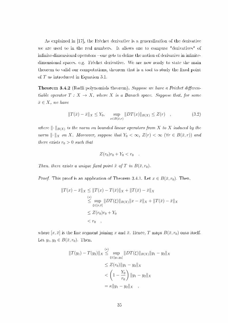
As explained in [17], the Fréchet derivative is a generalization of the derivative

we are used to in the real numbers. It allows one to compute "derivatives" of

in�nite-dimensional operators � one gets to de�ne the notion of derivative in in�nite-

dimensional spaces, e.g. Fréchet derivative. We are now ready to state the main

theorem to valid our computations, theorem that is a tool to study the �xed point

of T as introduced in Equation 3.1.

Theorem 3.4.2 (Radii polynomials theorem). Suppose we have a Fréchet di�eren-

tiable operator T : X → X, where X is a Banach space. Suppose that, for some

x ∈ X, we have

‖T (x)− x‖X ≤ Y0, supx∈B(x,r)

‖DT (x)‖B(X) ≤ Z(r) , (3.2)

where ‖· ‖B(X) is the norm on bounded linear operators from X to X induced by the

norm ‖· ‖X on X. Moreover, suppose that Y0 < ∞, Z(r) < ∞ (∀r ∈ B(x, r)) and

there exists r0 > 0 such that

Z(r0)r0 + Y0 < r0 .

Then, there exists a unique �xed point x of T in B(x, r0).

Proof. This proof is an application of Theorem 3.4.1. Let x ∈ B(x, r0). Then,

‖T (x)− x‖X ≤ ‖T (x)− T (x)‖X + ‖T (x)− x‖X(∗)≤ sup

ξ∈[x,x]

‖DT (ξ)‖B(X)‖x− x‖X + ‖T (x)− x‖X

≤ Z(r0)r0 + Y0

< r0 ,

where [x, x] is the line segment joining x and x. Hence, T maps B(x, r0) onto itself.

Let y1, y2 ∈ B(x, r0). Then,

‖T (y1)− T (y2)‖X(∗)≤ sup

ξ∈[y1,y2]

‖DT (ξ)‖B(X)‖y1 − y2‖X

≤ Z(r0)‖y1 − y2‖X

<

(1− Y0

r0

)‖y1 − y2‖X

= κ‖y1 − y2‖X ,

35

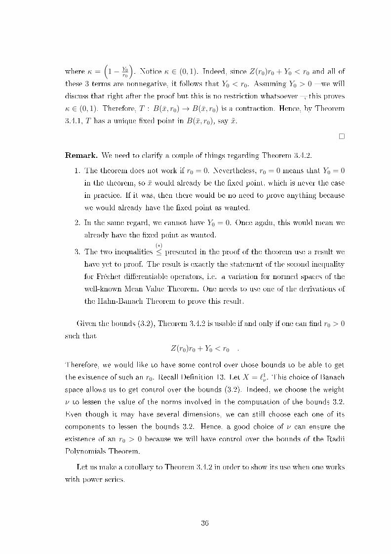
where κ =(

1− Y0r0

). Notice κ ∈ (0, 1). Indeed, since Z(r0)r0 + Y0 < r0 and all of

these 3 terms are nonnegative, it follows that Y0 < r0. Assuming Y0 > 0 � we will

discuss that right after the proof but this is no restriction whatsoever �, this proves

κ ∈ (0, 1). Therefore, T : B(x, r0)→ B(x, r0) is a contraction. Hence, by Theorem

3.4.1, T has a unique �xed point in B(x, r0), say x.

Remark. We need to clarify a couple of things regarding Theorem 3.4.2.

1. The theorem does not work if r0 = 0. Nevertheless, r0 = 0 means that Y0 = 0

in the theorem, so x would already be the �xed point, which is never the case

in practice. If it was, then there would be no need to prove anything because

we would already have the �xed point as wanted.

2. In the same regard, we cannot have Y0 = 0. Once again, this would mean we

already have the �xed point as wanted.

3. The two inequalities(∗)≤ presented in the proof of the theorem use a result we

have yet to proof. The result is exactly the statement of the second inequality

for Fréchet di�erentiable operators, i.e. a variation for normed spaces of the

well-known Mean Value Theorem. One needs to use one of the derivations of

the Hahn-Banach Theorem to prove this result.

Given the bounds (3.2), Theorem 3.4.2 is usable if and only if one can �nd r0 > 0

such that

Z(r0)r0 + Y0 < r0 .

Therefore, we would like to have some control over those bounds to be able to get

the existence of such an r0. Recall De�nition 13. Let X = `1ν . This choice of Banach

space allows us to get control over the bounds (3.2). Indeed, we choose the weight

ν to lessen the value of the norms involved in the computation of the bounds 3.2.

Even though it may have several dimensions, we can still choose each one of its

components to lessen the bounds 3.2. Hence, a good choice of ν can ensure the

existence of an r0 > 0 because we will have control over the bounds of the Radii

Polynomials Theorem.

Let us make a corollary to Theorem 3.4.2 in order to show its use when one works

with power series.

36

Corollary 3.4.1. Suppose we have a Fréchet di�erentiable operator T : X → X,

where X is a Banach space. Suppose that, for some x ∈ X, we have

‖T (x)− x‖X ≤ Y0, supx∈B(x,r)

‖DT (x)‖B(X) ≤ Z(r) = Z1 + Z2(r) ,

where ‖· ‖B(X) is the norm on bounded linear operators from X to X induced by the

norm ‖· ‖X on X. Moreover, suppose that Y0, Z1 < ∞, Z2(r) < ∞ (∀r ∈ B(x, r))

and there exists r0 > 0 such that

Z2(r0)r20 + (Z1 − 1)r0 + Y0 < 0 . (3.3)

Then, there exists a unique �xed point x of T in B(x, r0).

Proof. Notice

Z(r0) + Y0 < r0 ⇐⇒ Z2(r0)r20 + (Z1 − 1)r0 + Y0 < 0 .

Therefore, applying Theorem 3.4.2, we get the result.

Remark. Since Z2(r0), Z1, Y0 > 0 and r0 > 0, we must have Z1 < 1, otherwise r0

cannot be positive. In practice, we do not care too much about Z2(r0) and put a

lot of focus on Z1 to make sure it is less than 1. One can do so by diminishing

components of the weight ν and increasing the number of computed coe�cients.

Recall Operator 3.1. Assume X = `1,Nν . Since we are working on solving for

coe�cients of power series and A2 holds, the operator T will be given component-

wise by a �nite combination of Cauchy products � this fact will become clear in

Section 4. Hence, the same goes for its derivative � this fact will become clear in

Section 5. Recall Corollary 3.4.1. Let Z1 be a bound for the constant terms of the

derivative DT (x) � it does not depend on x. Let Z2(r) be a polynomial bound in

r for the higher order terms of DT (x) for all x ∈ B(x, r) � this fact will become

clear in Section 5. As stated in the above remark, Corollary 3.4.1 will be applicable

if there exists an r0 > 0 such that Equation 3.3 is veri�ed, i.e. if Z1 < 1. By the

current discussion, the left hand side of Equation 3.3 is going to be a polynomial in r

� substitute r0 for r. Hence, solving for r0 boils down to solving for the roots of the

latter polynomial. Therefore, given that the bound Y0 will be very small compared

to Z1 and Z2(r) � provided |ν| < 1 and N big enough �, we will have the existence

of a small r0 > 0 satisfying Equation 3.3. Thus, Theorem 3.4.2 is a powerful tool

37

for validating our computations because a �xed point of the operator T is a solution

for the coe�cients of the power series we are looking at.

Theorem 3.4.2 being stated, we are now ready to cover exactly which operators

we have to solve in practice (Section 4) and how we manage to use the theory on

Radii Polynomials to ensure we have good enough approximations of the power series

we are looking at (Section 5).

38

4 Practical operators

Theorem 3.4.2 provides us with existence and uniqueness of our power series

a posteriori. The Strong Implicit Function Theorem (see the Appendix) provides us

with existence and uniqueness of some of our power series � �xed point, eigenvalues

and eigenvectors (Subsections 4.1 and 4.2) � a priori. The Strong Implicit Function

Theorem is really important : It will provide us with analytic dependency of our

computations with respect to the parameters.

Recall (2.6). Recall our goal is to compute a parameterization, given by a power

series, of P . We want to compute the coe�cients of the power series of P . To do so,

we �rst need to compute parameterizations, given by power series, of the �xed point

x(ω) and the eigenvalues and eigenvectors of the Jacobian Matrix Dxf(x(ω), ω).

Then, we will be able to compute the parameterization of P . Therefore, we split

our computations into three parts, namely Subsections 4.1, 4.2 and 4.3.

Remark. Recall De�nitions 9, 12 and 13. Let X = (`1ν)l

(l > 0) with ν ∈ Rd (d >

0). Let α ∈ Zd, γ ∈ Zl and z ∈ X. Henceforth, for the sake of simplicity, we are

going to consider that

zα = 0 & zγii = 1 (i ∈ {1, . . . , l})

whenever αj < 0 for any j ∈ {1, . . . , d} and γi < 0 for any i ∈ {1, . . . , l}. This

remark is very useful when working with power series because it allows to disregard

negative indices as well as negative exponents of Cauchy products (see De�nition

12).

4.1 Fixed point operator

The �rst part of the method consists of the computation of a parameterization

of the �xed point x(ω) of the vector �eld of ODE (1.1) depending on the parameters

ω. By Assumption A2, suppose the vector �eld is parameterized by

f(x, ω) =

M2∑|γ2|=0

M1∑|γ1|=0

cγ1,γ2xγ1(ω − ω)γ2 . (4.1)

By Assumption A1, it has an hyperbolic �xed point xdef

= x(ω) for the value ω of the

parameters ω. Fixed points of the ODE (1.1) are zeros of the vector �eld. Therefore,

consider the equation

f(x, ω) = 0 . (4.2)

39

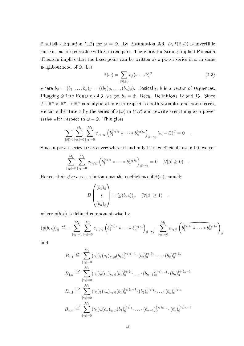
x satis�es Equation (4.2) for ω = ω. By Assumption A3, Dxf(x, ω) is invertible

since it has no eigenvalue with zero real part. Therefore, the Strong Implicit Function

Theorem implies that the �xed point can be written as a power series in ω in some

neighbourhood of ω. Let

x(ω) =∑|β|≥0

bβ(ω − ω)β (4.3)

where bβ = (b1, . . . , bn)β = ((b1)β, . . . , (bn)β). Basically, b is a vector of sequences.

Plugging ω into Equation 4.3, we get b0 = x. Recall De�nitions 12 and 15. Since

f : Rn × Rp → Rn is analytic at x with respect to both variables and parameters,

we can substitute x by the series of x(ω) in (4.2) and rewrite everything as a power

series with respect to ω − ω. This gives∑|β|≥0

M2∑|γ2|=0

M1∑|γ1|=0

cγ1,γ2

(b

(γ1)11 ∗ · · · ∗ b(γ1)n

n

)β−γ2

(ω − ω)β = 0 .

Since a power series is zero everywhere if and only if its coe�cients are all 0, we get

M2∑|γ2|=0

M1∑|γ1|=0

cγ1,γ2

(b

(γ1)11 ∗ · · · ∗ b(γ1)n

n

)β−γ2

= 0 (∀|β| ≥ 0) .

Hence, that gives us a relation onto the coe�cients of x(ω), namely

B

(b1)β...

(bn)β

= (g(b, c))β (∀|β| ≥ 1) ,

where g(b, c) is de�ned component-wise by

(g(b, c))βdef

= −M2∑|γ2|=1

M1∑|γ1|=0

cγ1,γ2

(b

(γ1)11 ∗ · · · ∗ b(γ1)n

n

)β−γ2−

M1∑|γ1|=0

cγ1,0

(b

(γ1)11 ∗ · · · ∗ b(γ1)n

n

)β

and

B1,1def

=

M1∑|γ1|=0

(γ1)1(c1)γ1,0(b1)(γ1)1−10 · (b2)

(γ1)20 · . . . · (bn)

(γ1)n0

B1,ndef

=

M1∑|γ1|=0

(γ1)n(c1)γ1,0(b1)(γ1)10 · . . . · (bn−1)

(γ1)n−1

0 · (bn)(γ1)n−10

Bn,1def

=

M1∑|γ1|=0

(γ1)1(cn)γ1,0(b1)(γ1)1−10 · (b2)

(γ1)20 · . . . · (bn)

(γ1)n0

Bn,ndef

=

M1∑|γ1|=0

(γ1)n(cn)γ1,0(b1)(γ1)10 · . . . · (bn−1)

(γ1)n−1

0 · (bn)(γ1)n−10

40

Bdef

=

B1,1 · · · B1,n

.... . .

...

Bn,1 · · · Bn,n

.

Thus, we can use this relation to get the recurrence relation

bβ = B−1 (g(b, c))β (∀|β| ≥ 1) . (4.4)

Let us justify the invertibility of B. Notice B = Dxf(x(ω), ω). By Assumption

A3, B has no eigenvalues with zero real part, so it is invertible.

The recurrence relation (4.4) requires an initial condition, which is b0. Notice

that

x(ω) = b0 .

Since the computation of x(ω) is the classic computation of �xed points of a vector

�eld, we know how to compute b0. Therefore, we have a way to compute exactly

the coe�cients of the power series of the �xed point x(ω). Recall the discussion

in Subsection 3.2, especially the de�nition of the general operator (3.1). Recall

De�nition 13. Assume we have computed all the coe�cients bβ up to order N − 1.

We are going to set T :(`1,Nµ

)n → (`1,Nµ

)nas

(T (u))βdef

=

0 if 0 ≤ |k| ≤ N − 1

B−1(g(b+ u, c)

)β

if |β| ≥ N, (4.5)

where

bβdef

=

bβ if 0 ≤ |β| ≤ N − 1

0 if |β| ≥ N.

We want to prove T has a unique �xed point and that u = 0 is a good approximation

of it. We have proven the existence of a series in ω for the �xed point x(ω), which

means that it has a radius of convergence R > 0 with R ∈ Rp. We know by basic

analysis that this implies

lim|β|→∞

|bβδβ| = 0 (−R < δ < R) ,

where δ ∈ Rp. Thus, we can get |bβδβ| as small as we want if we take |β| big enough.Notice that the terms |bβδβ| are exactly the terms involved in the

(`1,Nµ

)n-norm, just

substitute δ for µ. Hence, the(`1,Nµ

)n-norm of T (0) is going to be very small provided

N big enough. The latter is a blueprint to choose N : Choose N so that each |bβµβ|

41

is below some tolerance. This justi�es that u = 0 is a good approximation of the

�xed point of T in(`1,Nµ

)n. We say "the" because T is by de�nition the recurrence

relation, so the coe�cients of the series of x(ω) are a �xed point by de�nition of the

recurrence relation. Furthermore, they are the only �xed point because a solution

to the recurrence relation is totally determined by the initial condition.

Remark.

� For the sake of the argument, we assume here that the �xed point x(ω) is

isolated, i.e. not a cluster point with respect to the set of �xed points.

� Note that we do not prove the coe�cients bβ for |β| ≤ N − 1. Indeed, we

need not to because they have been computed exactly using the recurrence

relation, so there is no need to prove them.

Now that we know u = 0 is a good approximation of the unique �xed point of T

for some given tolerance, provided N big enough, it remains to rigorously prove it.

This is where we use Theorem 3.4.2, the Radii Polynomial Theorem. We just have

to compute the bounds (3.2). To ensure that the theorem works, we must ensure the

polynomial (3.3) has a positive root. To that end, we can take |µ| small enough and

N big enough. There is no proper ratio for the latters, their choice will be governed

by the needs for the proof and the software limitations.

4.2 Eigenvalues and eigenvectors operator

The second part consists of the computation of a parameterization of the

eigenvalues and eigenvectors of the vector �eld of the ODE (1.1) at the �xed point

x(ω). Assume we have already computed its parameterization with respect to ω,

i.e. we have already computed the coe�cients (4.4). Eigenvalues and eigenvectors

for the �xed point x(ω) around ω are zeros of the equation

DxF (x(ω), ω)v(ω)− λ(ω)v(ω) = 0 , (4.6)

where λ(ω) is an eigenvalue and v(ω) one of its eigenvectors for each value of the

parameters ω. Assume λ(ω) ∈ R � the complex case will be covered later on. Let

(λ, v)def

= (λ(ω), v(ω)) satisfy (4.6) at ω = ω. (λ, v) is an eigencouple � an eigenvalue

and one of its eigenvectors � by de�nition. The variables are λ and v1, . . . , vn, the

components of v. Since a scalar multiple of an eigenvector is again an eigenvector,

there are in�nitely many solutions to (4.6) at ω = ω, so there is no way to get

uniqueness of the eigenvector at ω = ω without at least another assumption.

42

Remark. An eigenvector has at least one nonzero component. Without loss of

generality, suppose vj 6= 0 (j ∈ {1, . . . , n}). Therefore, vvjis also an eigenvector of λ

because it is a scalar multiple of the eigenvector v and vj 6= 0.

Using the remark, without loss of generality, suppose that vj = 1. Thus, the

couple (λ, v) is the unique one to satisfy (4.6) at ω = ω. Indeed, the dimension

of the eigenspace of λ is one � it is a consequence of Assumption A3, namely the

eigenvalues are distinct.

Given vj = 1, since (4.6) has a unique solution at ω = ω, the Jacobian matrix

is invertible at ω = ω, so the Strong Implicit Function Theorem applies and we get

that λ(ω) and v(ω) can both be written as a series in ω in some neighbourhood of

ω. The fact that the Jacobian matrix is invertible can be derived from a straight

computation of the Jacobian matrix coupled with the assumption that the eigenspace

is of dimension one. We will come back shortly to that. Hence, let us write λ(ω)

and v(ω) as

λ(ω) =∑|β|≥0

λβ(ω − ω)β, v(ω) =∑|β|≥0

vβ(ω − ω)β ,

where vβ = (v1, . . . , vn)β = ((v1)β, . . . , (vn)β). Since vj(ω) = 1 and vj(ω) is analytic,

in particular continuous, there exists a neighbourhood of ω such that vj(ω) 6= 0

for all ω in this neighbourhood. Hence, without loss of generality, consider the

eigenvector V (ω) = v(ω)vj(ω)

. It is a power series depending on ω around ω because it

is holomorphic in the neighbourhood of ω (see [18]). Therefore, we now have

λ(ω) =∑|β|≥0

λβ(ω − ω)β, V (ω) =∑|β|≥0

Vβ(ω − ω)β , (4.7)

where Vβ = (V1, . . . , Vn)β = ((V1)β, . . . , (Vn)β). Noticing that Vj(ω) = 1 for all ω in

a proper neighbourhood of ω, we deduce that

(Vj)β =

1 , if |β| = 0

0 , otherwise.

In the end, we have isolated the couple (λ(ω), V (ω)) with respect to the eigenspace

depending on ω. As for the computation of the coe�cients (4.4), by substituting

(4.7) into (4.6), we get

43

∑|β|≥0

M2∑|γ2|=0

M1∑|γ1|=0

cγ1,γ2

((γ1)1

(b

(γ1)1−11 ∗ b(γ1)2

2 ∗ · · · ∗ b(γ1)nn ∗ V1

)β−γ2

+ · · ·+

(γ1)n

(b

(γ1)11 ∗ · · · ∗ b(γ1)n−1

n−1 ∗ b(γ1)n−1n ∗ Vn

)β−γ2

)(ω − ω)β −

∑|β|≥0

(λ ∗ V )β(ω − ω)β = 0

,

where b is de�ned as in Subsection 4.1 and c is de�ned as in Equation 4.1. For the

sake of simplicity, let V∗jλ = (V1, . . . , Vj−1, λ, Vj+1, . . . , Vn). Since a power series is

zero everywhere if and only if its coe�cients are all 0, we get the relation

B(V∗jλ )β = B

(V1)β...

(Vj−1)β

λβ

(Vj+1)β...

(Vn)β

=(g(V

∗jλ , Vj, b, c)

)β

(∀|β| ≥ 1) ,

where g(V∗jλ , Vj, b, c) is de�ned component-wise by

(g1(V

∗jλ , Vj , b, c)

)β

def

= −M2∑|γ2|=1

M1∑|γ1|=0

cγ1,γ2∑

1≤i≤n

(γ1)i(b(γ1)11 ∗ · · · ∗ b(γ1)i−1

i−1 ∗ b(γ1)i−1i ∗ b(γ1)i+1

i+1 ∗ · · · ∗ b(γ1)nn ∗ Vi)β−γ2

(g2(V

∗jλ , Vj , b, c)

)β

def

= −M1∑|γ1|=0

cγ1,0

(γ1)j(b(γ1)11 ∗ · · · ∗ b(γ1)j−1

j−1 ∗ b(γ1)j−1j ∗ b(γ1)j+1

j+1 ∗ · · · ∗ b(γ1)nn ∗ Vj)β

+∑

1≤i≤ni6=j

(γ1)i(b(γ1)11 ∗ · · · ∗ b(γ1)i−1

i−1 ∗ b(γ1)i−1i ∗ b(γ1)i+1

i+1 ∗ · · · ∗ b(γ1)nn ∗ Vi)β

(g3(V

∗jλ , Vj , b, c)

)β

def

= −M1∑|γ1|=0

cγ1,0∑

1≤i≤ni6=j

(γ1)i

((γ1)1(b1)

(γ1)1−10 (b2)

(γ1)20 · · · (bi−1)

(γ1)i−1

0 (bi)(γ1)i−10 (bi+1)

(γ1)i+1

0 · · · (bn)(γ1)n0 (Vi)0(b1)β

+ · · ·+ ((γ1)i − 1)(b1)(γ1)10 · · · (bi−1)

(γ1)i−1

0 (bi)(γ1)i−20 (bi+1)

(γ1)i+1

0 · · · (bn)(γ1)n0 (Vi)0(bi)β

+ · · ·+ (γ1)n(b1)(γ1)10 · · · (bi−1)

(γ1)i−1

0 (bi)(γ1)i−10 (bi+1)

(γ1)i+1

0 · · · (bn−1)(γ1)n−1

0 (bn)(γ1)n−10 (Vi)0(bn)β

)(g4(V

∗jλ , Vj , b, c)

)β

def

= (λ∗V )β + λ0(Vj)β · ej(g(V

∗jλ , Vj , b, c)

)β

def

=(g1(V

∗jλ , Vj , b, c)

)β

+(g2(V

∗jλ , Vj , b, c)

)β

+(g3(V

∗jλ , Vj , b, c)

)β

+(g4(V

∗jλ , Vj , b, c)

)β

,

44

ej is the j-th canonical vector from Rn and B is given column-wise by

Bdef

=

K1 · · · Kj−1 Kj Kj+1 · · · Kn

−

λ0

. . .

λ0

0

λ0

. . .

λ0

︸︷︷︸

i-th column

with

Bidef

=

M1∑|γ1|=0

(γ1)i· cγ1,0· (b1)(γ1)10 · · · (bi−1)

(γ1)i−1

0 · (bi)(γ1)i−10 · (bi+1)

(γ1)i+1

0 · · · (bn)(γ1)n0 , if i 6= j

−V0 , if i = j

.

Thus, we can use this relation to get the recurrence relation

(V∗jλ )β = B−1

(g(V

∗jλ , Vj, b, c)

)β

(∀|β| ≥ 1) . (4.8)

Let us justify the invertibility of B. Let K = DxF (x(ω), ω) − λ(ω)· In. Recall

(λ, v) = (λ(ω), v(ω)) satis�es Equation 4.6. Let Vdef

= V0. It follows (λ, V ) also

satis�es Equation 4.6. Notice the columns of B andK are the same but the i-th ones.

Since the kernel ofK is of dimension one by AssumptionA3, we know all its columns

but the i-th one are linearly independent. Therefore, if B is not invertible, then its

i-th column is a linear combination of the others. Denote by B1, . . . , Bn its columns

from �rst to last respectively. Since Bj = −V , there exits k1, . . . , kj−1, kj+1, . . . , kn ∈R such that V = k1B1 + · · · + kj−1Bj−1 + kj+1Bj+1 + · · · + knBn. Thus, V belongs

to the image of K. Let y ∈ Rn be such that Ky = V . We have

K2y = K(Ky) = KV = 0 .

Hence, y is a generalized vector of DxF (x(ω), ω) for the eigenvalue λ. However, the

dimension of the eigenspace of λ is one because the kernel of K is of dimension one.

Therefore, y is a multiple of V , say y = κV (κ ∈ R), and we have

V = Ky = K(κV ) = κKV = κ· 0 = 0 .

45

This is a contradiction because an eigenvector is not zero by de�nition. Thereby, B

is invertible.

The recurrence relation (4.8) requires an initial condition, which is (V∗jλ )0. Notice

λ(ω) = λ0, V (ω) = V0 .

We can use classic computations to get (λ0, V0) = (λ, V ). Indeed, V0 is the unique

eigenvector associated to the eigenvalue λ0 such that (Vj)0 = 1 because the dimen-

sion of the eigenspace of λ0 is one. Therefore, we have a way to compute exactly

the coe�cients of both the power series of the eigenvalue λ(ω) and its associated

eigenvector V (ω). Recall the discussion in Subsection 3.2, especially the de�nition

of the general operator (3.1). Recall De�nition 13. Assume we have computed all

the coe�cients (V∗jλ )β up to order N − 1. We are going to set T :

(`1,Nµ

)n → (`1,Nµ

)nas

(T (u))βdef

=

0 , if 0 ≤ |β| ≤ N − 1

B−1(g(V

∗jλ + u, Vj, b, c)

)β

, if |β| ≥ N, (4.9)

where

(V∗jλ )β = (V1, . . . , Vj−1, λ, Vj+1, . . . , Vn)β

def

=

(V∗jλ )β , if 0 ≤ |β| ≤ N − 1

0 , if |β| ≥ N

and

(Vj)βdef

=

1 , if |β| = 0

0 , otherwise.

The goal will be to prove that T has a unique �xed point and that u = 0 is a good

approximation of it. We have two power series that have a radius of convergence

R > 0 � without loss of generality, we can assume they both have the same radius of

convergence � and T is by de�nition the recurrence relation. Hence, using the same

argument as for the �xed point in Subsection 4.1, we can get the bounds (3.2) as

small as we want by take |µ| small enough and N big enough. Therefore, Theorem

3.4.2 will apply and we will have existence and uniqueness of both the power series

for the eigenvalue and its associated eigenvector.

Remark. Since it is going to become handy for the next computations, we suppose

the eigenvalue does not change sign within its neighbourhood of de�nition around

ω. It is always going to be the case if we shrink this neighbourhood enough.

46

Note we have to repeat this procedure for every eigenvalue and their associated

eigenvector before moving on to the computation of the parameterizations of the

stable and unstable manifolds.

4.3 Stable and unstable manifolds coe�cients operator

The third part consists of the computation of a parameterization of P (see

Equation 2.6) around the value ω of the parameters. Assume we have already com-

puted the parameterization with respect to ω of the �xed point and the eigenvalues

and eigenvectors, i.e. we have already computed the coe�cients (4.4) and (4.8).

Recall Theorem 2.3.1 and Equation (2.7). Assume P : Rk × Rp → Rn is given by a

power series, say

P (θ, ω) =∑|β|≥0

∑|α|≥0

aα,βθα(ω − ω)β . (4.10)

Let us motivate this assumption. Recall Assumptions A1, A2 and A3. We have

an ODE with a polynomial vector �eld. By Theorem 2.2.2, for any �xed value

of the parameters ω, there exists a parameterization of the local stable manifold

W sloc

(x(ω)) at x(ω) that is analytic and whose domain is a subset of the stable

subspace Es containing the origin. This motivates the power series for P .

We assume Equations (2.6) stand. The �rst two equations are consequences of

Theorem 2.2.2. The third one is an assumption that leads to Equations (2.7) of

Theorem 2.3.1. These equations allow us to retrieve a recurrence relation over the

coe�cients of the power series of P . Among them, the only restrictive assumption

is the third equation of Equations (2.6). However, recall that it is similar to the

Hartman-Grobmann Theorem (see [4]), so it is sort of natural to make it.

Recall we assume that P is given by (4.10) and the vector �eld (1.1) is given by

f(x, ω) =∑M2

|γ2|=0

∑M1

|γ1|=0 cγ1,γ2(x − x)γ1(ω − ω)γ2 . Substituting the power series of

P into the homological equation in (2.7), we get

M2∑|γ2|=0

M1∑|γ1|=0

cγ1,γ2

(a

(γ1)11 ∗ · · · ∗ a(γ1)n

n

)α,β−γ2

=((α· λ) ∗ aα

)β

(4.11)

wherever it is de�ned. Note that c is de�ned as in Equation 4.1 and λ as in Subsection

4.2. Hence, that gives us a relation onto the coe�cients of P (θ, ω), namely

(A− (α·λ)0· In

)(a1)α,β

...

(an)α,β

=(g(a, λ, c)

)α,β

(∀|α| ≥ 2, |β| ≥ 0) , (4.12)

47

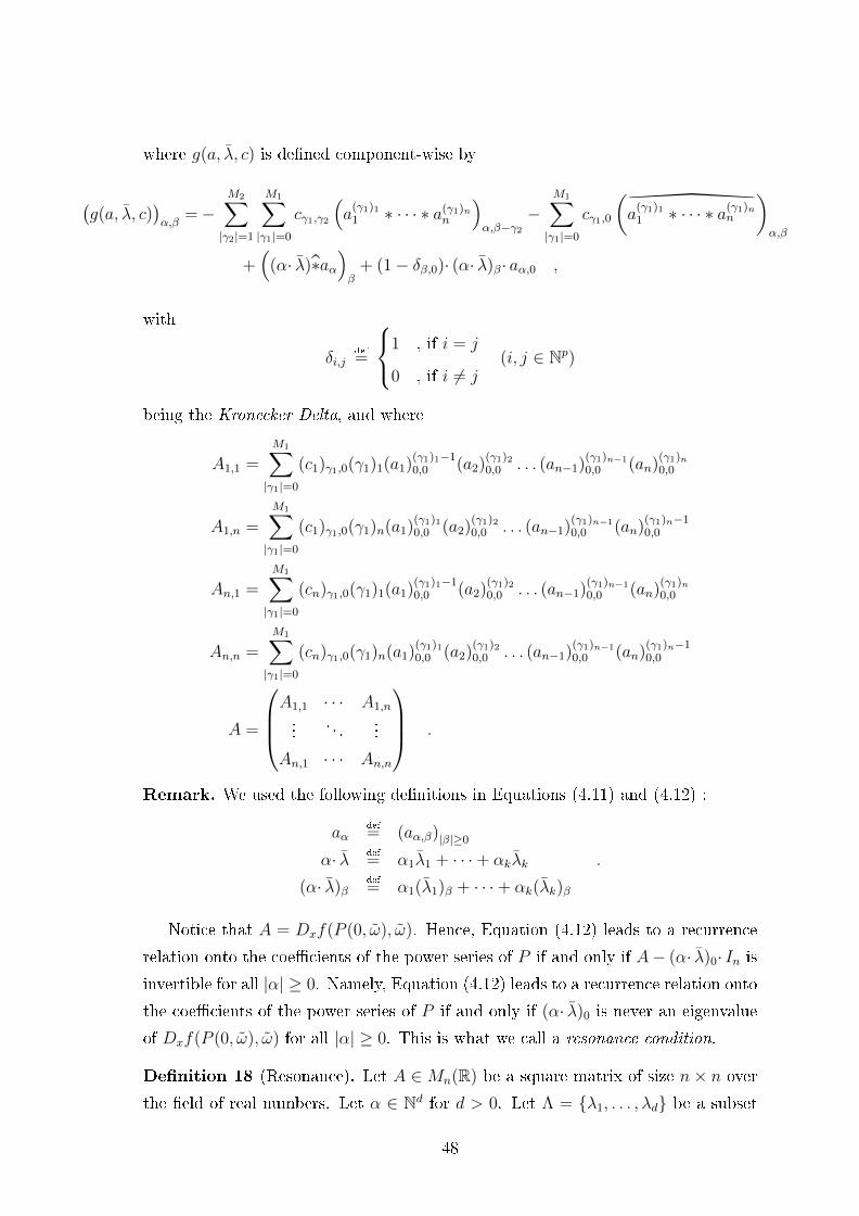
where g(a, λ, c) is de�ned component-wise by

(g(a, λ, c)

)α,β

=−M2∑|γ2|=1

M1∑|γ1|=0

cγ1,γ2

(a

(γ1)11 ∗ · · · ∗ a(γ1)n

n

)α,β−γ2

−M1∑|γ1|=0

cγ1,0

(a

(γ1)11 ∗ · · · ∗ a(γ1)n

n

)α,β

+(

(α· λ)∗aα)β

+ (1− δβ,0)· (α· λ)β· aα,0 ,

with

δi,jdef

=

1 , if i = j

0 , if i 6= j(i, j ∈ Np)

being the Kronecker Delta, and where

A1,1 =

M1∑|γ1|=0

(c1)γ1,0(γ1)1(a1)(γ1)1−10,0 (a2)

(γ1)20,0 . . . (an−1)

(γ1)n−1

0,0 (an)(γ1)n0,0

A1,n =

M1∑|γ1|=0

(c1)γ1,0(γ1)n(a1)(γ1)10,0 (a2)

(γ1)20,0 . . . (an−1)

(γ1)n−1

0,0 (an)(γ1)n−10,0

An,1 =

M1∑|γ1|=0

(cn)γ1,0(γ1)1(a1)(γ1)1−10,0 (a2)

(γ1)20,0 . . . (an−1)

(γ1)n−1

0,0 (an)(γ1)n0,0

An,n =

M1∑|γ1|=0

(cn)γ1,0(γ1)n(a1)(γ1)10,0 (a2)

(γ1)20,0 . . . (an−1)

(γ1)n−1

0,0 (an)(γ1)n−10,0

A =

A1,1 · · · A1,n

.... . .

...

An,1 · · · An,n

.

Remark. We used the following de�nitions in Equations (4.11) and (4.12) :

aαdef

= (aα,β)|β|≥0

α· λ def

= α1λ1 + · · ·+ αkλk .

(α· λ)βdef

= α1(λ1)β + · · ·+ αk(λk)β

Notice that A = Dxf(P (0, ω), ω). Hence, Equation (4.12) leads to a recurrence

relation onto the coe�cients of the power series of P if and only if A− (α· λ)0· In isinvertible for all |α| ≥ 0. Namely, Equation (4.12) leads to a recurrence relation onto

the coe�cients of the power series of P if and only if (α· λ)0 is never an eigenvalue

of Dxf(P (0, ω), ω) for all |α| ≥ 0. This is what we call a resonance condition.

De�nition 18 (Resonance). Let A ∈ Mn(R) be a square matrix of size n× n over

the �eld of real numbers. Let α ∈ Nd for d > 0. Let Λ = {λ1, . . . , λd} be a subset

48

of the eigenvalues of A. We say the matrix A has a resonance on Λ if there is an

eigenvalue of A that is a nonnegative integer linear combination � an integer linear

combination such that all the integers are nonnegative � of the eigenvalues of A

belonging to Λ.

We mention here that the resonance condition of Equation 4.12 is formulated

only with the negative eigenvalues of the derivative Dxf(x(ω), ω) of the vector �eld

(1.1) at the �xed point (x(ω), ω). Like in dynamical systems, we see that the study

of the eigenvalues of the linearized system at a �xed point is a primordial asset.

Moreover, it is a phenomena that often arises when one is looking at conjugacy

relations with parameterizations given by power series (see [2] and [1]).

As mentioned in Section 1, we were missing one assumption :

A4. Dxf(x(ω), ω) has no resonance on Λ = {λ1, . . . , λk}.Thus, we can use Equation 4.12 to get the recurrence relation

aα,β = (A− (α· λ)0· In)−1(g(a, λ, c)

)α,β

(∀|α| ≥ 2, |β| ≥ 0) . (4.13)

Let us justify the invertibility of A − (α· λ)0· In for all |α| ≥ 2. Assumption A4

states A has no resonance on the set of negative eigenvalues. Therefore, the matrix

A−(α· λ)0· In is invertible for all |α| ≥ 0. In particular, it is invertible for all |α| ≥ 2.

The recurrence relation (4.13) has the initial conditions

a0,β = bβ, aei,β = V iβ (∀1 ≤ i ≤ j) ,

where ei ∈ Nk is the vector with all components equal to 0 except for the i-th one

that is equal to 1, bβ are de�ned as in Subsection 4.1 and V iβ are the coe�cients

of the power series of the i-th eigenvector at the �xed point x(ω) � the eigenvector

associated to the i-th negative eigenvalue �, computed as in Subsection 4.2. Those

initial conditions are derived from the �rst two equations of (2.4). Therefore, we

have a way to compute exactly the coe�cients of the series of P . However, as

opposed to Subsections 4.1 and 4.2, the invertible matrix does depend on the index

of the coe�cients. As we will see in Section 5, this causes an issue concerning the

computation of the bounds (3.2). To make up for it, we need to modify slightly

g(a, c) to introduce an intermediate operator.

De�nition 19. Let a1, . . . , an ∈ `1ν,µ. We de�ne a1 ? · · · ? an component-wise by

(a1 ? · · · ? an)α,βdef

= (a1 ∗ · · · ∗ an)α,β − ((a1)α ∗ (a2)0 ∗ · · · ∗ (an)0)β

− · · · − ((a1)0 ∗ · · · ∗ (an−1)0 ∗ (an)α)β.

49

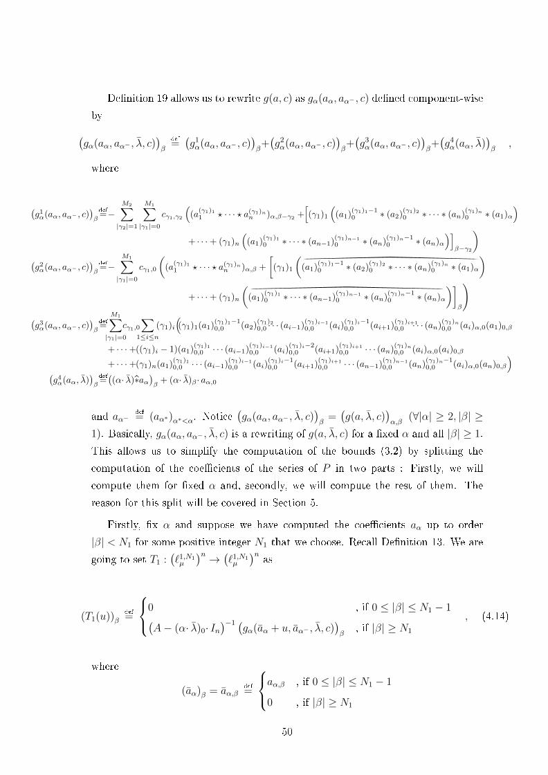
De�nition 19 allows us to rewrite g(a, c) as gα(aα, aα− , c) de�ned component-wise

by(gα(aα, aα− , λ, c)

)β

def

=(g1α(aα, aα− , c)

)β+(g2α(aα, aα− , c)

)β+(g3α(aα, aα− , c)

)β+(g4α(aα, λ)

)β

,

where

(g1α(aα, aα− , c)

)β

def

=−M2∑|γ2|=1

M1∑|γ1|=0

cγ1,γ2

((a

(γ1)11 ? · · · ? a(γ1)nn )α,β−γ2 +

[(γ1)1

((a1)

(γ1)1−10 ∗ (a2)

(γ1)20 ∗ · · · ∗ (an)

(γ1)n0 ∗ (a1)α

)+ · · ·+ (γ1)n

((a1)

(γ1)10 ∗ · · · ∗ (an−1)

(γ1)n−1

0 ∗ (an)(γ1)n−10 ∗ (an)α

)]β−γ2

)(g2α(aα, aα− , c)

)β

def

=−M1∑|γ1|=0

cγ1,0

((a

(γ1)11 ? · · · ? a(γ1)nn )α,β +

[(γ1)1

((a1)

(γ1)1−10 ∗ (a2)

(γ1)20 ∗ · · · ∗ (an)

(γ1)n0 ∗ (a1)α

)

+ · · ·+ (γ1)n

((a1)

(γ1)10 ∗ · · · ∗ (an−1)

(γ1)n−1

0 ∗ (an)(γ1)n−10 ∗ (an)α

)]β

)(g3α(aα, aα− , c)

)β

def

=

M1∑|γ1|=0

cγ1,0∑

1≤i≤n

(γ1)i

((γ1)1(a1)

(γ1)1−10,0 (a2)

(γ1)20,0 · · · (ai−1)

(γ1)i−1

0,0 (ai)(γ1)i−10,0 (ai+1)

(γ1)i+1

0,0 · · · (an)(γ1)n0,0 (ai)α,0(a1)0,β

+ · · ·+((γ1)i − 1)(a1)(γ1)10,0 · · · (ai−1)

(γ1)i−1

0,0 (ai)(γ1)i−20,0 (ai+1)

(γ1)i+1

0,0 · · · (an)(γ1)n0,0 (ai)α,0(ai)0,β

+ · · ·+(γ1)n(a1)(γ1)10,0 · · · (ai−1)

(γ1)i−1

0,0 (ai)(γ1)i−10,0 (ai+1)

(γ1)i+1

0,0 · · · (an−1)(γ1)n−1

0,0 (an)(γ1)n−10,0 (ai)α,0(an)0,β

)(g4α(aα, λ)

)β

def

=((α· λ)∗aα

)β

+ (α· λ)β · aα,0

and aα−def

= (aα∗)α∗<α. Notice(gα(aα, aα− , λ, c)

)β

=(g(a, λ, c)

)α,β

(∀|α| ≥ 2, |β| ≥1). Basically, gα(aα, aα− , λ, c) is a rewriting of g(a, λ, c) for a �xed α and all |β| ≥ 1.

This allows us to simplify the computation of the bounds (3.2) by splitting the

computation of the coe�cients of the series of P in two parts : Firstly, we will

compute them for �xed α and, secondly, we will compute the rest of them. The

reason for this split will be covered in Section 5.

Firstly, �x α and suppose we have computed the coe�cients aα up to order

|β| < N1 for some positive integer N1 that we choose. Recall De�nition 13. We are

going to set T1 :(`1,N1µ

)n → (`1,N1µ

)nas

(T1(u))βdef

=

0 , if 0 ≤ |β| ≤ N1 − 1(A− (α· λ)0· In

)−1 (gα(aα + u, aα− , λ, c)

)β

, if |β| ≥ N1

, (4.14)

where

(aα)β = aα,βdef

=

aα,β , if 0 ≤ |β| ≤ N1 − 1

0 , if |β| ≥ N1

50

and

aα−def

= (aα∗)α∗<α & (aα∗)β = aα∗,βdef

=

aα∗,β , if 0 ≤ |β| ≤ N1 − 1

0 , if |β| ≥ N1

(α∗ < α) .

Remark. aα + u means that u ∈(`1,N1µ

)nis added only to aα and not to aα∗ for

α∗ < α.

The goal will be to prove that T1 has a unique �xed point and that u = 0 is a

good approximation of it. We know that the series has two radius of convergence,

say, R1, R2 > 0, the �rst one being for the convergence in θ and the second one for

the convergence in ω. Moreover, T1 is by de�nition the recurrence relation (4.13)

for α �xed so, using the same argument as for the �xed point and the eigenvalues

and eigenvectors, we can get the bounds (3.2) as small as we want by taking |µ|small enough and N1 big enough, whence Theorem 3.4.2 will apply and we will have

existence and uniqueness of the series for the �xed α. Notice we have to repeat the

computations for every α. Since we can only do a �nite number of computations,

we will have to set a new operator to prove the existence and uniqueness of the

remaining coe�cients of P .

Remark. Even if α is �xed, the recurrence relation 4.13 still depends on every

coe�cients aα∗ such that α∗ < α. Moreover, at some point, each component of aα

is 0 for every α that we �x ; we take it to be past order N1 − 1 without loss of

generality.

Secondly, suppose that we have computed a rigorous approximation of the coef-

�cients aα,β for every |α| < N2 where N2 is a positive integer that we choose, i.e.

we successfully applied Theorem 3.4.2 to every aα such that |α| < N2. We are now

going to set T2 :(`1,N2ν,µ

)n → (`1,N2ν,µ

)nas

(T2(u))α,βdef

=

0 , if 0 ≤ |α| ≤ N2 − 1(A− (α· λ)0· In

)−1 (g(a+ u, λ, c)

)α,β

, if |α| ≥ N2

, (4.15)

where

aα,β =

aα,β , if 0 ≤ |α| ≤ N2 − 1 & 0 ≤ |β| ≤ N1 − 1

0 , otherwise.

51

We again want to prove that u = 0 is a good approximation of the �xed point of T2.

Since T2 is the recurrence relation 4.13, by the same argument as for the �xed point

and the eigenvalues and eigenvectors, we will have control over the bounds (3.2) by

taking N2 big enough and both |ν| and |µ| small enough. Hence, Theorem 3.4.2 will

apply and we will get existence and uniqueness of the series of P .

Remark.

� In practice, we want to take |ν| as big as possible because we will get a biggerradius of convergence for the power series of P .

� Recall Subsection 2.3. For the unstable manifold, the same argument applies

with Λu(ω) instead of Λs(ω) and it will yield the same kind of operator.

Furthermore, the computations of the bounds (3.2) is going to be almost the

same as for the stable manifold, so there is no need to go over it in details.

Let us come back on the complex case. Suppose the eigenvalues of Subsection

4.2 are complex � they can be a mix of real and complex ones. The argument of

Subsections 4.2 and 4.3 still applies by taking the absolute values |· | as the complex

absolute values. Nonetheless, we will end up with a complex parameterization P of

the local stable manifold. Fortunately, there is a way to retrieve a real parameteri-

zation of P out of the complex one. Sort the eigenvalues such that λ1, . . . , λj are the

complex ones and λj+1, . . . , λk the real ones. Since Dxf(x(ω), ω) is a real matrix, we

know the complex eigenvalues are complex conjugate, i.e. they come in pair. Sort

again the complex eigenvalues such that λ1 = λ2, . . . , λj−1 = λj � here, z denotes

the conjugate of z ∈ C. De�ne Q : Rk × Rp → Rn as

Q(ϕ, ω)def

= P ((ϕ1 + i·ϕ2), . . . , (ϕj−1 + i·ϕj), ϕj+1, . . . , ϕk, ω) .

Now, notice

aα1,α2,...,αj−1,αj ,αj+1,...,αk,β = aα2,α1,...,αj ,αj−1,αj+1,...,αk,β (∀|α| ≥ 2, |β| ≥ 0) .

Indeed, recall V i is the eigenvector associated to the i-th eigenvalue and ei is the

i-th canonical unit vector of Rk. Notice V 1 = V 2, . . . , V j−1 = V j, aei = V i (∀1 ≤i ≤ k) and aα,β is given by a recurrence relation depending only on coe�cients of

lesser order. One can verify that those facts together imply the above equation.

Furthermore, the above equation implies that

Q(ϕ, ω) = Q(ϕ, ω) ,

52

i.e. Q is a real parameterization of the local stable manifold. Thus, our method also

works for the complex case, it just requires the extra step of de�ning Q as above.

The next section will cover how one can estimate the bounds (3.2) for the oper-

ators of Section 4. Then, two examples will follow in Section 6 to apply our theory

in practice.

53

5 Bounds

As mentioned in Subsection 3.4, when using power series as parameterizations

of the objects we are computing � �xed point, eigenvalues and eigenvectors and

parameterization of the local stable manifold �, in order to apply Theorem 3.4.2,

we need to make sure Equation 3.3 holds. In practice, this means we need sharp

estimates for some of the bounds (3.2) and coarse estimates for the others. As

mentioned brie�y in Subsection 3.2, the bound Y0 is already going to be small by

de�nition of T , the operator we are working with. Indeed, regardless of which one

of the operators from Section 4 we work with, it has its components equal to 0 up to

a certain order. Therefore, since our norms from De�nition 14 all include a weight,

taking each component of the latter less than 1 and small enough, we have the norm

of T (0) − 0 as small as we want. This is precisely a justi�cation to the bound Y0

being as small as desired.

Y0 being a positive number as close to 0 as needed, the polynomials from Equation

3.3 will have a positive root close to 0 if Z1 − 1 is negative, i.e. Z1 < 1. In practice,

since the bound Z1 is the bound for the linear terms of our operator T , we need to

be sharper on it so it does not exceed 1. However, regarding the bound Z2(r), in

general, one can just take a coarse bound of it without any consequences.

For the sake of simplicity, let us make a de�nition that limits the notation used

regarding matrices.

De�nition 20 (Matrix operator). Let X be any of the spaces from De�nition 13.

Let h ∈ X and A be a matrix of size m × m over the �eld of real numbers. The

matrix operator A : X → X is a linear functional whose action on h ∈ X is given

by (Ah)δ

= A·hδ .

If δ = (α, β) and A depends α, i.e. A = A(α), then the matrix operator A(α) : X →X is a linear functional whose action on h ∈ X is given by(

A(α)h)α,β

def

= A(α)·hα,β .

Remark. We are going to use the same symbol for a matrix and its matrix operator.

It is always going to be clear whether it is used for the matrix or the matrix operator.

For a norm ‖· ‖X on a Banach space X, we are going to denote the norm induced

by ‖· ‖X of a bounded linear operator from X to X by ‖· ‖B(X). Since it is going to

be useful for the computation of the bounds (3.2), let us make a theorem.

54

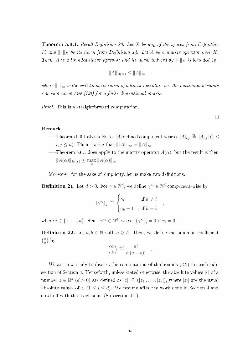
Theorem 5.0.1. Recall De�nition 20. Let X be any of the spaces from De�nition

13 and ‖· ‖X be its norm from De�nition 14. Let A be a matrix operator over X.

Then, A is a bounded linear operator and its norm induced by ‖· ‖X is bounded by

‖A‖B(X) ≤ ‖A‖∞ ,

where ‖· ‖∞ is the well-know∞-norm of a linear operator, i.e. the maximum absolute

row sum norm (see [19]) for a �nite dimensional matrix.

Proof. This is a straightforward computation.

Remark.

� Theorem 5.0.1 also holds for |A| de�ned component-wise as |A|i,j def

= |Ai,j| (1 ≤i, j ≤ n). Then, notice that ‖ |A| ‖∞ = ‖A‖∞.

� Theorem 5.0.1 does apply to the matrix operator A(α), but the result is then

‖A(α)‖B(X) ≤ maxα‖A(α)‖∞.

Moreover, for the sake of simplicity, let us make two de�nitions.

De�nition 21. Let d > 0. For γ ∈ Nd, we de�ne γ∗i ∈ Nd component-wise by

(γ∗i)kdef

=

γk , if k 6= i

γk − 1 , if k = i,

where i ∈ {1, . . . , d}. Since γ∗i ∈ Nd, we set (γ∗i)i = 0 if γi = 0.

De�nition 22. Let a, b ∈ N with a ≥ b. Then, we de�ne the binomial coe�cient(ab

)by (a

b

)def

=a!

b!(a− b)! .

We are now ready to discuss the computation of the bounds (3.2) for each sub-

section of Section 4. Henceforth, unless stated otherwise, the absolute values |· | of anumber z ∈ Rd (d > 0) are de�ned as |z| def

= (|z1|, . . . , |zd|), where |zi| are the usualabsolute values of zi (1 ≤ i ≤ d). We resume after the work done in Section 4 and

start o� with the �xed point (Subsection 4.1).

55

5.1 Fixed Point

Recall the operator T :(`1,Nµ

)n → (`1,Nµ

)ngiven by (4.5). Its derivative

DT (u) :(`1,Nµ

)n → (`1,Nµ

)nevaluated at an element u ∈

(`1,Nµ

)nis a linear operator.

One can verify its action on an element h ∈(`1,Nµ

)nis given by

(DT (u)h)β = B−1(Dug(b+ u, c)h

)β

, (5.1)

where

(Dug(b+ u, c)h

)β

=−M2∑|γ2|=1

M1∑|γ1|=0

cγ1,γ2 ·[

(γ1)1·(

(b1 + u1)(γ1)1−1 ∗ (b2 + u2)(γ1)2 ∗ · · · ∗ (bn + un)(γ1)n ∗ h1)

+ · · ·+ (γ1)n·(

(b1 + u1)(γ1)1 ∗ · · · ∗ (bn−1 + un−1)(γ1)n−1 ∗ (bn + un)(γ1)n−1 ∗ hn) ]

β−γ2

−M1∑|γ1|=0

cγ1,0·[(γ1)1·

((b1 + u1)(γ1)1−1 ∗ (b2 + u2)(γ1)2 ∗ · · · ∗ (bn + un)(γ1)n ∗ h1)

+ · · ·+ (γ1)n·(

(b1 + u1)(γ1)1 ∗ · · · ∗ (bn−1 + un−1)(γ1)n−1 ∗ (bn + un)(γ1)n−1 ∗ hn)]β

.

Recall the bounds (3.2). Recall De�nition 14. Y0 is given by

Y0def

= ‖T (0)− 0‖(n)1,µ,N = ‖T (0)‖(n)

1,µ,N . (5.2)

Notice the computation of Y0 involves a �nite number of terms because b is a sequence

with �nitely many nonzero elements and T is evaluated at u = 0.

Let us move on to the computation of Z(r). Notice

‖DT (u)h‖(n)1,µ,N ≤ ‖B−1‖B((`1,Nµ )

n)· ‖Dug(b+ u, c)h‖(n)

1,µ,N .

By Theorem 5.0.1, we have

‖DT (u)h‖(n)1,µ,N ≤ ‖B−1‖∞· ‖Dug(b+ u, c)h‖(n)

1,µ,N .

Therefore, what remains to bound is ‖Dug(b+ u, c)h‖(n)1,µ,N .

Lemma 5.1.1. Recall (5.1) and De�nitions 16, 21 and 22. Let r > 0. Suppose

‖u‖(n)1,µ,N ≤ r and ‖h‖(n)

1,µ,N = 1. We have

‖Dug(b+ u, c)h‖(n)1,µ,N ≤ Zg(r) ,

where

56

Zg(r)def

= max

M2∑|γ2|=1

µγ2M1∑|γ1|=0

|cγ1,γ2 |

|(γ1)1|∑η≤γ∗11

((γ∗11 )1η1

)· · ·(

(γ∗11 )nηn

)‖b1‖(γ

∗11 )1−η1

1,µ · · · ‖bn‖(γ∗11 )n−ηn

1,µ r|η|

+ · · ·+ |(γ1)n|∑η≤γ∗n1

((γ∗n1 )1η1

)· · ·(

(γ∗n1 )nηn

)‖b1‖(γ

∗n1 )1−η1

1,µ · · · ‖bn‖(γ∗n1 )n−ηn

1,µ r|η|

+

M1∑|γ1|=0

|cγ1,0|

|(γ1)1|∑η≤γ∗11

((γ∗11 )1η1

)· · ·(

(γ∗11 )nηn

)‖b1‖(γ

∗11 )1−η1

1,µ · · · ‖bn‖(γ∗11 )n−ηn

1,µ r|η|

+ · · ·+ |(γ1)n|∑η≤γ∗n1

((γ∗n1 )1η1

)· · ·(

(γ∗n1 )nηn

)‖b1‖(γ

∗n1 )1−η1

1,µ · · · ‖bn‖(γ∗n1 )n−ηn

1,µ r|η|

.

(5.3)

Proof. Let(Dug(b+ u, c)h

)β

= (D1(u)h)β + (D2(u)h)β, where D1(u)h and D2(u)h

are de�ned component-wise by

(D1(u)h)βdef

= −M2∑|γ2|=1

M1∑|γ1|=0

cγ1,γ2 ·[

(γ1)1·(

(b1 + u1)(γ1)1−1 ∗ (b2 + u2)(γ1)2 ∗ · · · ∗ (bn + un)(γ1)n ∗ h1)

+ · · ·+ (γ1)n·((b1 + u1)(γ1)1 ∗ · · · ∗ (bn−1 + un−1)(γ1)n−1 ∗ (bn + un)(γ1)n−1 ∗ hn

) ]β−γ2

and

(D2(u)h)βdef

= −M1∑|γ1|=0

cγ1,0·[(γ1)1·

((b1 + u1)(γ1)1−1 ∗ (b2 + u2)(γ1)2 ∗ · · · ∗ (bn + un)(γ1)n ∗ h1)

+ · · ·+ (γ1)n·(

(b1 + u1)(γ1)1 ∗ · · · ∗ (bn−1 + un−1)(γ1)n−1 ∗ (bn + un)(γ1)n−1 ∗ hn)]β

.

Let Υ1(u, h) =∑|β|≥0

∣∣∣(D1(u)h)β

∣∣∣µβ. We have

Υ1(u, h) =∑|β|≥0

∣∣∣∣∣∣M2∑|γ2|=1

M1∑|γ1|=0

cγ1,γ2 ·[

(γ1)1·(

(b1 + u1)(γ1)1−1 ∗ (b2 + u2)(γ1)2 ∗ · · · ∗ (bn + un)(γ1)n ∗ h1)

+ · · ·+ (γ1)n·((b1 + u1)(γ1)1 ∗ · · · ∗ (bn−1 + un−1)(γ1)n−1 ∗ (bn + un)(γ1)n−1 ∗ hn

) ]β−γ2

∣∣∣∣∣∣µβ≤

M2∑|γ2|=1

µγ2M1∑|γ1|=0

|cγ1,γ2 |∑|β|≥0

[|(γ1)1|·

∣∣∣(b1 + u1)(γ1)1−1 ∗ (b2 + u2)(γ1)2 ∗ · · · ∗ (bn + un)(γ1)n ∗ h1∣∣∣

+ · · ·+ |(γ1)n|·∣∣(b1 + u1)(γ1)1 ∗ · · · ∗ (bn−1 + un−1)(γ1)n−1 ∗ (bn + un)(γ1)n−1 ∗ hn

∣∣ ]β−γ2

µβ−γ2 .

The change of order of summation was possible because the triple series converges

absolutely. Let i ∈ {1, . . . , n}. Notice

57

(b1 + u1)(γ1)1−1 ∗ · · · ∗ (bi−1 + ui−1)(γ1)i−1 ∗ (bi + ui)(γ1)i−1 ∗ (bi+1 + ui+1)(γ1)i+1 ∗ · · · ∗ (bn + un)(γ1)n ∗ hi

=∑η≤γ∗i1

((γ∗i1 )1η1

)· · ·(

(γ∗i1 )nηn

)· b(γ

∗i1 )1−η1

1 ∗ uη11 ∗ · · · ∗ b(γ∗i1 )n−ηn

n ∗ uηnn ∗ hi .

Hence, using Proposition 3.3.1 along with ‖u‖(n)1,µ,N ≤ r and ‖h‖(n)

1,µ,N = 1, we get

Υ1(u, h) ≤M2∑|γ2|=1

µγ2M1∑|γ1|=0

|cγ1,γ2 |

|(γ1)1|∑η≤γ∗11

((γ∗11 )1η1

)· · ·(

(γ∗11 )nηn

)‖b1‖(γ

∗11 )1−η1

1,µ · · · ‖bn‖(γ∗11 )n−ηn

1,µ r|η|

+ · · ·+ |(γ1)n|∑η≤γ∗n1

((γ∗n1 )1η1

)· · ·(

(γ∗n1 )nηn

)‖b1‖(γ

∗n1 )1−η1

1,µ · · · ‖bn‖(γ∗n1 )n−ηn

1,µ r|η|

.

Moreover, let Υ2(u, h) =∑|β|≥0

∣∣∣(D2(u)h)β

∣∣∣µβ. We have

Υ2(u, h) =∑|β|≥0

∣∣∣∣∣∣M1∑|γ1|=0

cγ1,0·[(γ1)1·

((b1 + u1)(γ1)1−1 ∗ (b2 + u2)(γ1)2 ∗ · · · ∗ (bn + un)(γ1)n ∗ h1)

+ · · ·+ (γ1)n·(

(b1 + u1)(γ1)1 ∗ · · · ∗ (bn−1 + un−1)(γ1)n−1 ∗ (bn + un)(γ1)n−1 ∗ hn)]β

∣∣∣∣∣∣µβ≤

M1∑|γ1|=0

|cγ1,0|∑|β|≥0

[|(γ1)1|·

∣∣∣(b1 + u1)(γ1)1−1 ∗ (b2 + u2)(γ1)2 ∗ · · · ∗ (bn + un)(γ1)n ∗ h1∣∣∣+ · · ·+ |(γ1)n|·

∣∣∣(b1 + u1)(γ1)1 ∗ · · · ∗ (bn−1 + un−1)(γ1)n−1 ∗ (bn + un)(γ1)n−1 ∗ hn∣∣∣]βµβ .

The change of order of summation was possible because the double series converges

absolutely. Let i ∈ {1, . . . , n}. Notice

(b1 + u1)(γ1)1−1 ∗ · · · ∗ (bi−1 + ui−1)(γ1)i−1 ∗ (bi + ui)(γ1)i−1 ∗ (bi+1 + ui+1)(γ1)i+1 ∗ · · · ∗ (bn + un)(γ1)n ∗ hi

=∑η≤γ∗i1

((γ∗i1 )1η1

)· · ·(

(γ∗i1 )nηn

)· b(γ

∗i1 )1−η1

1 ∗ uη11 ∗ · · · ∗ b(γ∗i1 )n−ηn

n ∗ uηnn ∗ hi .

Hence, using Theorem 3.3.2 along with ‖u‖(n)1,µ,N ≤ r and ‖h‖(n)

1,µ,N = 1, we get

Υ2(u, h) ≤M1∑|γ1|=0

|cγ1,0|

|(γ1)1|∑η≤γ∗11

((γ∗11 )1η1

)· · ·(

(γ∗11 )nηn

)‖b1‖(γ

∗11 )1−η1

1,µ · · · ‖bn‖(γ∗11 )n−ηn

1,µ r|η|

+ · · ·+ |(γ1)n|∑η≤γ∗n1

((γ∗n1 )1η1

)· · ·(

(γ∗n1 )nηn

)‖b1‖(γ

∗n1 )1−η1

1,µ · · · ‖bn‖(γ∗n1 )n−ηn

1,µ r|η|

.

58

Finally, the result follows from

‖Dug(b+ u, c)h‖(n)1,µ,N ≤ max

{Υ1(u, h) + Υ2(u, h)

}≤ Zg(r) .

We can now apply the Radii Polynomials Approach (see Subsection 3.4) to see

what are the conditions needed for the operator T :(`1,Nµ

)n → (`1,Nµ

)ngiven by (4.5)

to have a �xed point close to u = 0.

Theorem 5.1.1. Recall T :(`1,Nµ

)n → (`1,Nµ

)n, the operator given by (4.5). Let K def

=

‖B−1‖∞. Recall the bounds Y0 and Zg(r) de�ned in (5.2) and (5.3) respectively. Let

Z1def

= K·max

M2∑|γ2|=1

µγ2M1∑|γ1|=0

|cγ1,γ2 |(|(γ1)1|· ‖b1‖(γ

∗11 )1

1,µ · · · ‖bn‖(γ∗11 )n

1,µ + · · ·+ |(γ1)n|· ‖b1‖(γ∗n1 )1

1,µ · · · ‖bn‖(γ∗n1 )n

1,µ

)

+

M1∑|γ1|=0

|cγ1,0|(|(γ1)1|· ‖b1‖(γ

∗11 )1

1,µ · · · ‖bn‖(γ∗11 )n

1,µ + · · ·+ |(γ1)n|· ‖b1‖(γ∗n1 )1

1,µ · · · ‖bn‖(γ∗n1 )n

1,µ

)(5.4)

and

Z2(r)def

= K·Zg(r)− Z1 . (5.5)

If there exists r0 > 0 such that

Z2(r0)r20 + (Z1 − 1)r0 + Y0 < 0 , (5.6)

then T has a unique �xed point in B(0, r0).

Proof. This is an application of Corollary 3.4.1 using Lemma 5.1.1 and the bounds

Y0, Z1 and Z2(r) de�ned in (5.2), (5.4) and (5.5) respectively.

Remark. The reason for the use of the bounds Z1 (Equation 5.4) and Z2(r) (Equa-

tion 5.5) instead of the bound Z(r)def

= K·Zg(r) (Equation 5.3) is going to be

explained in Subsection 5.4.

Assuming the existence of an r0 > 0 satisfying Theorem 5.1.1 � this matter is

going to be addressed in Subsection 5.4 �, we can now move on to the computation

of the bounds (3.2) for the eigenvalues and eigenvectors (Subsection 4.2).

59

5.2 Eigenvalues and eigenvectors

Recall the operator T :(`1,Nµ

)n → (`1,Nµ

)ngiven by (4.9). Its derivative

DT (u) :(`1,Nµ

)n → (`1,Nµ

)nevaluated at an element u ∈

(`1,Nµ

)nis a linear operator.

Its action on an element h ∈(`1,Nµ

)nis given by

(DT (u)h)β = B−1(Dug(V

∗jλ + u, Vj, b, c)h

)β

, (5.7)

where

(Dug(V

∗jλ +u, Vj , b, c)h

)β

def

= −M2∑|γ2|=1

M1∑|γ1|=0

cγ1,γ2∑

1≤i≤ni6=j

(γ1)i

(b(γ1)11 ∗ · · · ∗ b(γ1)i−1

i−1 ∗ b(γ1)i−1i ∗ b(γ1)i+1

i+1 ∗ · · · ∗ b(γ1)nn ∗ hi)β−γ2

−M1∑|γ1|=0

cγ1,0∑

1≤i≤ni6=j

(γ1)i

(b(γ1)11 ∗ · · · ∗ b(γ1)i−1

i−1 ∗ b(γ1)i−1i ∗ b(γ1)i+1

i+1 ∗ · · · ∗ b(γ1)nn ∗ hi)β

+(Vj ∗hj)β · ej +∑

1≤i≤ni6=j

(((Vi + ui)∗hj

)β

+((λ+ uj)∗hi

)β

)· ei ,

with ei (i ∈ {1, . . . , n}) being the i-th canonical vector from Rn. Recall the bounds

(3.2). Recall De�nition 14. Y0 is given by

Y0def

= ‖T (0)− 0‖(n)1,µ,N = ‖T (0)‖(n)

1,µ,N . (5.8)

Notice the computation of Y0 involves a �nite number of terms because b, Vj and

V∗jλ are sequences with �nitely many nonzero elements and T is evaluated at u = 0.

Let us move on to the computation of Z(r). Notice

‖DT (u)h‖(n)1,µ,N ≤ ‖B−1‖B((`1,Nµ )

n)· ‖Dug(V

∗jλ + u, Vj, b, c)h‖(n)

1,µ,N .

By Theorem 5.0.1, we have

‖DT (u)h‖(n)1,µ,N ≤ ‖B−1‖∞· ‖Dug(V

∗jλ + u, Vj, b, c)h‖(n)

1,µ,N .

Therefore, what remains to bound is ‖Dug(V∗jλ + u, Vj, b, c)h‖(n)

1,µ,N .

Lemma 5.2.1. Recall (5.7) and De�nitions 16 and 21. Let r > 0. Suppose

‖u‖(n)1,µ,N ≤ r and ‖h‖(n)

1,µ,N = 1. We have

‖Dug(V∗jλ + u, Vj, b, c)h‖(n)

1,µ,N ≤ Zg(r) ,

where

60

Zg(r)def

= max

M2∑|γ2|=1

µγ2M1∑|γ1|=0

|cγ1,γ2|∑1≤i≤ni6=j

|(γ1)i|· ‖b1‖(γ∗i1 )1

1,µ · · · ‖bn‖(γ∗i1 )n

1,µ

+

M1∑|γ1|=0

|cγ1,0|∑1≤i≤ni6=j

|(γ1)i|· ‖b1‖(γ∗i1 )1

1,µ · · · ‖bn‖(γ∗i1 )n

1,µ

+∑1≤i≤ni 6=j

(‖Vi‖1,µ + ‖λ‖1,µ + 2r

)· ei

.

(5.9)

Proof. Let(Dug(V

∗jλ + u, Vj, b, c)h

)β

= (D1(u)h)β + (D2(u)h)β, where D1(u)h and

D2(u)h are de�ned component-wise by

(D1(u)h)βdef

= −M2∑|γ2|=1

M1∑|γ1|=0

cγ1,γ2∑

1≤i≤ni6=j

(γ1)i

(b(γ1)11 ∗ · · · ∗ b(γ1)i−1

i−1 ∗ b(γ1)i−1i ∗ b(γ1)i+1

i+1 ∗ · · · ∗ b(γ1)nn ∗ hi)β−γ2

and

(D2(u)h)βdef

= −M1∑|γ1|=0

cγ1,0∑

1≤i≤ni6=j

(γ1)i

(b(γ1)11 ∗ · · · ∗ b(γ1)i−1

i−1 ∗ b(γ1)i−1i ∗ b(γ1)i+1

i+1 ∗ · · · ∗ b(γ1)nn ∗ hi)β

+(Vj ∗hj)β · ej +∑

1≤i≤ni6=j

(((Vi + ui)∗hj

)β

+((λ+ uj)∗hi

)β

)· ei

.

Let Υ1(u, h) =∑|β|≥0

∣∣∣(D1(u)h)β

∣∣∣µβ. We have

Υ1(u, h) =∑|β|≥0

∣∣∣∣∣∣∣M2∑|γ2|=1

M1∑|γ1|=0

cγ1,γ2∑

1≤i≤ni6=j

(γ1)i

(b(γ1)11 ∗ · · · ∗ b(γ1)i−1

i−1 ∗ b(γ1)i−1i ∗ b(γ1)i+1

i+1 ∗ · · · ∗ b(γ1)nn ∗ hi)β−γ2

∣∣∣∣∣∣∣µβ≤

M2∑|γ2|=1

µγ2M1∑|γ1|=0

|cγ1,γ2 |∑

1≤i≤ni6=j

|(γ1)i|∑|β|≥0

∣∣∣∣(b(γ1)11 ∗ · · · ∗ b(γ1)i−1

i−1 ∗ b(γ1)i−1i ∗ b(γ1)i+1

i+1 ∗ · · · ∗ b(γ1)nn ∗ hi)β−γ2

∣∣∣∣µβ−γ2 .

The change of order of summation was possible because the quadruple series con-

verges absolutely. Let i ∈ {1, . . . , n}. Notice

b(γ1)11 ∗ · · · ∗ b(γ1)i−1

i−1 ∗ b(γ1)i−1i ∗ b(γ1)i+1

i+1 ∗ · · · ∗ b(γ1)nn ∗ hi = b

(γ∗i1 )1

1 ∗ · · · ∗ b(γ∗i1 )n

n ∗ hi .

Hence, using Proposition 3.3.1 along with ‖h‖(n)1,µ,N = 1, we get

61

Υ1(u, h) ≤M2∑|γ2|=1

µγ2M1∑|γ1|=0

|cγ1,γ2|∑1≤i≤ni6=j

|(γ1)i|· ‖b1‖(γ∗i1 )1

1,µ · · · ‖bn‖(γ∗i1 )n

1,µ .

Moreover, let Υ2(u, h) =∑|β|≥0

∣∣∣(D2(u)h)β

∣∣∣µβ. We have

Υ2(u, h)def

=∑|β|≥0

∣∣∣∣∣∣∣M1∑|γ1|=0

cγ1,0∑

1≤i≤ni6=j

(γ1)i

(b(γ1)11 ∗ · · · ∗ b(γ1)i−1

i−1 ∗ b(γ1)i−1i ∗ b(γ1)i+1

i+1 ∗ · · · ∗ b(γ1)nn ∗ hi)β

+(Vj ∗hj)β · ej +∑

1≤i≤ni6=j

(((Vi + ui)∗hj

)β

+((λ+ uj)∗hi

)β

)· ei

∣∣∣∣∣∣∣µβ≤

M1∑|γ1|=0

|cγ1,0|∑

1≤i≤ni6=j

|(γ1)i|∑|β|≥0

∣∣∣∣∣(b(γ1)11 ∗ · · · ∗ b(γ1)i−1

i−1 ∗ b(γ1)i−1i ∗ b(γ1)i+1

i+1 ∗ · · · ∗ b(γ1)nn ∗ hi)β

∣∣∣∣∣µβ+∑

1≤i≤ni6=j

∑|β|≥0

∣∣∣(((Vi + ui)∗hj)β

+((λ+ uj)∗hi

)β

)· ei∣∣∣µβ .

The change of order of summation was possible because the triple and double series

both converge absolutely. Else, we used the fact that (Vj ∗hj)β = 0 (|β| ≥ 0) by

de�nition of Vj (see Subsection 4.2). Let i ∈ {1, . . . , n}. Notice

b(γ1)11 ∗ · · · ∗ b(γ1)i−1

i−1 ∗ b(γ1)i−1i ∗ b(γ1)i+1

i+1 ∗ · · · ∗ b(γ1)nn ∗ hi = b

(γ∗i1 )1

1 ∗ · · · ∗ b(γ∗i1 )n

n ∗ hi

and

(Vi + ui)∗hj = Vi∗hj + ui∗hj & (λ+ uj)∗hi = λ∗hi + uj ∗hi .

Hence, using Theorem 3.3.2 along with ‖u‖(n)1,µ,N ≤ r and ‖h‖(n)

1,µ,N = 1, we get

Υ2(u, h) ≤M1∑|γ1|=0

|cγ1,0|∑1≤i≤ni 6=j

|(γ1)i|· ‖b1‖(γ∗i1 )1

1,µ · · · ‖bn‖(γ∗i1 )n

1,µ

+∑1≤i≤ni6=j

(‖Vi‖1,µ + ‖λ‖1,µ + 2r

)· ei

.

Finally, the result follows from

‖Dug(V∗jλ + u, Vj, b, c)h‖(n)

1,µ,N ≤ max{

Υ1(u, h) + Υ2(u, h)}≤ Zg(r) .

62

We can now apply the Radii Polynomials Approach (see Subsection 3.4) to see

what are the conditions needed for the operator T :(`1,Nµ

)n → (`1,Nµ

)ngiven by (4.9)

to have a �xed point close to u = 0.

Theorem 5.2.1. Recall T :(`1,Nµ

)n → (`1,Nµ

)n, the operator given by (4.9). Let K def

=

‖B−1‖∞. Recall the bounds Y0 and Zg(r) de�ned in (5.8) and (5.9) respectively. Let

Z1def

= K·max

M2∑|γ2|=1

µγ2M1∑|γ1|=0

|cγ1,γ2|∑1≤i≤ni6=j

|(γ1)i|· ‖b1‖(γ∗i1 )1

1,µ · · · ‖bn‖(γ∗i1 )n

1,µ

+

M1∑|γ1|=0

|cγ1,0|∑1≤i≤ni 6=j

|(γ1)i|· ‖b1‖(γ∗i1 )1

1,µ · · · ‖bn‖(γ∗i1 )n

1,µ

+∑1≤i≤ni6=j

(‖Vi‖1,µ + ‖λ‖1,µ

)· ei

(5.10)

and

Z2(r)def

= K·Z(r)− Z1 . (5.11)

If there exists r0 > 0 such that

Z2(r0)r20 + (Z1 − 1)r0 + Y0 < 0 , (5.12)

then T has a unique �xed point in B(0, r0).

Proof. This is an application of Corollary 3.4.1 using Lemma 5.2.1 and the bounds

Y0, Z1 and Z2(r) de�ned in (5.8), (5.10) and (5.11) respectively.

Remark. The reason for the use of the bounds Z1 (Equation 5.10) and Z2(r) (Equa-

tion 5.11) instead of the bound Z(r)def

= K·Zg(r) (Equation 5.9) is going to be

explained in Subsection 5.4.

Assuming the existence of an r0 > 0 satisfying Theorem 5.2.1 � this matter is

going to be addressed in Subsection 5.4 �, we can now move on to the computa-

tion of the bounds (3.2) for the coe�cients of the stable and unstable manifolds

parameterizations (Subsection 4.3).

63

5.3 Stable and unstable manifolds coe�cients

As opposed to Subsections 5.1 and 5.2, this subsection is going to address the

computation of the bounds (3.2) for two operators instead of one, namely the two

operators of Subsection 4.3.

Recall the operator T1 :(`1,N1µ

)n → (`1,N1µ

)ngiven by (4.14). Its derivative

DT1(u) :(`1,N1µ

)n → (`1,N1µ

)nevaluated at an element u ∈

(`1,N1µ

)nis a linear opera-

tor. Its action on an element h ∈(`1,N1µ

)nis given by

(DT1(u)h)β =(A− (α· λ)0· In

)−1 (Dugα(aα + u, aα− , λ, c)h

)β

, (5.13)

where

(Dugα(aα + u, aα− , λ, c)h

)β

= −M2∑|γ2|=1

M1∑|γ1|=0

cγ1,γ2

[(γ1)1

((a1)

(γ1)1−10 ∗ (a2)

(γ1)20 ∗ · · · ∗ (an)

(γ1)n0 ∗ h1

)+ · · ·+ (γ1)n

((a1)

(γ1)10 ∗ · · · ∗ (an−1)

(γ1)n−1

0 ∗ (an)(γ1)n−10 ∗ hn

) ]β−γ2

−M1∑|γ1|=0

cγ1,0

[(γ1)1

((a1)

(γ1)1−10 ∗ (a2)

(γ1)20 ∗ · · · ∗ (an)

(γ1)n0 ∗ h1

)+ · · ·+ (γ1)n

((a1)

(γ1)10 ∗ · · · ∗ (an−1)

(γ1)n−1

0 ∗ (an)(γ1)n−10 ∗ hn

)]β

+((α· λ)∗h

)β

.

Recall the bounds (3.2). Let (Y1)0 = Y0 and Z1(r) = Z(r). Recall De�nition 14.

(Y1)0 is given by

(Y1)0def

= ‖T1(0)− 0‖(n)1,µ,N1

= ‖T1(0)‖(n)1,µ,N1

. (5.14)

Notice the computation of (Y1)0 involves a �nite number of terms because λ, aα−

and aα are sequences with �nitely many nonzero elements and T1 is evaluated at

u = 0.

Let us move on to the computation of Z1(r). Notice

‖DT1(u)h‖(n)1,µ,N1

≤∥∥∥ (A− (α· λ)0· In

)−1∥∥∥B((`1,N1µ )

n) · ‖Dugα(aα+u, aα− , λ, c)h‖(n)1,µ,N1

.

By Theorem 5.0.1, we have

‖DT1(u)h‖(n)1,µ,N1

≤∥∥∥ (A− (α· λ)0· In

)−1∥∥∥∞· ‖Dugα(aα + u, aα− , λ, c)h‖(n)

1,µ,N1.

Notice∥∥∥ (A− (α· λ)0· In

)−1∥∥∥∞

is a constant because α is �xed for the operator T1.

Therefore, what remains to bound is ‖Dugα(aα + u, aα− , λ, c)h‖(n)1,µ,N1

.

64

Lemma 5.3.1. Recall (5.13) and De�nitions 16 and 21. Let r > 0. Suppose

‖u‖(n)1,µ,N1

≤ r and ‖h‖(n)1,µ,N1

= 1. We have

‖Dugα(aα + u, aα− , λ, c)h‖(n)1,µ,N1

≤ Zg1 (r) ,

where

Zg1 (r)

def

= max

M2∑|γ2|=1

µγ2M1∑|γ1|=0

|cγ1,γ2|∑

1≤i≤n

|(γ1)i|· ‖(a1)0‖(γ∗i1 )1

1,µ · · · ‖(an)0‖(γ∗i1 )n

1,µ

+

M1∑|γ1|=0

|cγ1,0|∑

1≤i≤n

|(γ1)i|· ‖(a1)0‖(γ∗i1 )1

1,µ · · · ‖(an)0‖(γ∗i1 )n

1,µ

+ α· ‖λ‖1,µ

(5.15)

with

α· ‖λ‖1,µdef

= α1· ‖λ1‖1,µ + · · ·+ αk· ‖λk‖1,µ .

Proof. Let(Dugα(aα + u, aα− , λ, c)h

)β

= (D1(u)h)β +(D2(u)h)β, where D1(u)h and

D2(u)h are de�ned component-wise by

(D1(u)h)βdef

= −M2∑|γ2|=1

M1∑|γ1|=0

cγ1,γ2

[(γ1)1

((a1)

(γ1)1−10 ∗ (a2)

(γ1)20 ∗ · · · ∗ (an)

(γ1)n0 ∗ h1

)+ · · ·+ (γ1)n

((a1)

(γ1)10 ∗ · · · ∗ (an−1)

(γ1)n−1

0 ∗ (an)(γ1)n−10 ∗ hn

) ]β−γ2

and

(D2(u)h)βdef

= −M1∑|γ1|=0

cγ1,0

[(γ1)1

((a1)

(γ1)1−10 ∗ (a2)

(γ1)20 ∗ · · · ∗ (an)

(γ1)n0 ∗ h1

)+ · · ·+ (γ1)n

((a1)

(γ1)10 ∗ · · · ∗ (an−1)

(γ1)n−1

0 ∗ (an)(γ1)n−10 ∗ hn

)]β

+((α· λ)∗h

)β

.

Let Υ1(u, h) =∑|β|≥0

∣∣∣(D1(u)h)β

∣∣∣µβ. We have

65

Υ1(u, h) =∑|β|≥0

∣∣∣∣∣∣M2∑|γ2|=1

M1∑|γ1|=0

cγ1,γ2

[(γ1)1

((a1)

(γ1)1−10 ∗ (a2)

(γ1)20 ∗ · · · ∗ (an)

(γ1)n0 ∗ h1

)

+ · · ·+ (γ1)n

((a1)

(γ1)10 ∗ · · · ∗ (an−1)

(γ1)n−1

0 ∗ (an)(γ1)n−10 ∗ hn

) ]β−γ2

∣∣∣∣∣∣µβ

≤M2∑|γ2|=1

M1∑|γ1|=0

|cγ1,γ2 |

|(γ1)1|∑|β|≥0

∣∣∣∣((a1)(γ1)1−10 ∗ (a2)

(γ1)20 ∗ · · · ∗ (an)

(γ1)n0 ∗ h1

)β−γ2

∣∣∣∣µβ+ · · ·+ |(γ1)n|

∑|β|≥0

∣∣∣∣((a1)(γ1)10 ∗ · · · ∗ (an−1)

(γ1)n−1

0 ∗ (an)(γ1)n−10 ∗ hn

)β−γ2

∣∣∣∣µβ .

The change of order of summation was possible because the two triple series both

converge absolutely. Let i ∈ {1, . . . , n}. Notice

(a1)(γ1)10 ∗· · ·∗(ai−1)

(γ1)i−1

0 ∗(ai)(γ1)i−10 ∗(ai+1)(γ1)i+1

0 ∗· · ·∗(an)(γ1)n0 ∗hi = (a1)

(γ∗i1 )1

0 ∗· · ·∗(an)(γ∗i1 )n

0 ∗hi .

Hence, using Proposition 3.3.1 along with ‖h‖(n)1,µ,N1

= 1, we get

Υ1(u, h) ≤M2∑|γ2|=1

µγ2M1∑|γ1|=0

|cγ1,γ2|∑

1≤i≤n

|(γ1)i|· ‖(a1)0‖(γ∗i1 )1

1,µ · · · ‖(an)0‖(γ∗i1 )n

1,µ .

Moreover, let Υ2(u, h) =∑|β|≥0

∣∣∣(D2(u)h)β

∣∣∣µβ. We have

Υ2(u, h) =∑|β|≥0

∣∣∣∣∣∣M1∑|γ1|=0

cγ1,0

[(γ1)1

((a1)

(γ1)1−10 ∗ (a2)

(γ1)20 ∗ · · · ∗ (an)

(γ1)n0 ∗ h1

)+ · · ·+ (γ1)n

((a1)

(γ1)10 ∗ · · · ∗ (an−1)

(γ1)n−1

0 ∗ (an)(γ1)n−10 ∗ hn

)]β

+((α· λ)∗h

)β

∣∣∣∣∣∣µβ≤

M1∑|γ1|=0

|cγ1,0|

|(γ1)1|∑|β|≥0

∣∣∣∣∣(

(a1)(γ1)1−10 ∗ (a2)

(γ1)20 ∗ · · · ∗ (an)

(γ1)n0 ∗ h1

)β

∣∣∣∣∣µβ+ · · ·+ |(γ1)n|

∑|β|≥0

∣∣∣∣∣(

(a1)(γ1)10 ∗ · · · ∗ (an−1)

(γ1)n−1

0 ∗ (an)(γ1)n−10 ∗ hn

)β

∣∣∣∣∣µβ

+∑|β|≥0

∣∣∣((α· λ)∗h)β

∣∣∣µβ .

66

The change of order of summation was possible because the two double series both

converge absolutely, as well as the single series. Let i ∈ {1, . . . , n}. Notice

(a1)(γ1)10 ∗ · · · ∗ (ai−1)

(γ1)i−1

0 ∗ (ai)(γ1)i−10 ∗ (ai+1)

(γ1)i+1

0 ∗ · · · ∗ (an)(γ1)n0 ∗ hi = (a1)

(γ∗i1 )1

0 ∗ · · · ∗ (an)(γ∗i1 )n

0 ∗ hi .

Let 1def

= (1, . . . , 1) ∈ Rn. Hence, using Theorem 3.3.2 along with ‖h‖(n)1,µ,N1

= 1, we

get

Υ2(u, h) ≤M1∑|γ1|=0

|cγ1,0|∑

1≤i≤n

|(γ1)i|· ‖(a1)0‖(γ∗i1 )1

1,µ · · · ‖(an)0‖(γ∗i1 )n

1,µ

+ 1·(α· ‖λ‖1,µ

) .

Finally, the result follows from

‖Dugα(aα + u, aα− , λ, c)h‖(n)1,µ,N1

≤ max{

Υ1(u, h) + Υ2(u, h)}≤ Zg

1 (r) .

We can now apply the Radii Polynomials Approach (see Subsection 3.4) to see

what are the conditions needed for the operator T1 :(`1,N1µ

)n → (`1,N1µ

)ngiven by

(4.14) to have a �xed point close to u = 0.

Theorem 5.3.1. Recall T1 :(`1,N1µ

)n → (`1,N1µ

)n, the operator given by (4.14). Let

Kdef

=∥∥∥ (A− (α· λ)0· In

)−1∥∥∥∞. Recall the bounds (Y1)0 and Zg

1 (r) de�ned in (5.14)

and (5.15) respectively. Let

Z1(r)def

= K·Zg1 (r) . (5.16)

If there exists r0 > 0 such that

(Z1(r)− 1)r0 + (Y1)0 < 0 , (5.17)

then T1 has a unique �xed point in B(0, r0).

Proof. This is an application of Theorem 3.4.2 using Lemma 5.3.1 and the bounds

(Y1)0 and Z1(r) de�ned in (5.14) and (5.16) respectively.

67

Remark. Notice the bound Z1(r) is constant, i.e. it does not depend on r. There-

fore, the left hand side of Equation 5.17 is a polynomial of degree 1.

Assuming the existence of an r0 > 0 satisfying Theorem 5.3.1 � this matter is

going to be addressed in Subsection 5.4 �, we can now address the computation of

the bounds (3.2) for the second operator of Subsection 4.3.

Recall the operator T2 :(`1,N2ν,µ

)n → (`1,N2ν,µ

)ngiven by (4.15). Its derivative

DT2(u) :(`1,N2ν,µ

)n → (`1,N2ν,µ

)nevaluated at an element u ∈

(`1,N2ν,µ

)nis a linear opera-

tor. Its action on an element h ∈(`1,N2ν,µ

)nis given by

(DT2(u)h)α,β =(A− (α· λ)0· In

)−1 (Dug(a+ u, λ, c)h

)α,β

, (5.18)

where

(D1ug(a+ u, λ, c)h

)α,β

def

= −M2∑|γ2|=1

M1∑|γ1|=0

cγ1,γ2 ·[

(γ1)1·(

(a1 + u1)(γ1)1−1 ∗ (a2 + u2)(γ1)2 ∗ · · · ∗ (an + un)(γ1)n ∗ h1)

+ · · ·+ (γ1)n·((a1 + u1)(γ1)1 ∗ · · · ∗ (an−1 + un−1)(γ1)n−1 ∗ (an + un)(γ1)n−1 ∗ hn

) ]α,β−γ2

−M1∑|γ1|=0

cγ1,0·[(γ1)1·

((a1 + u1)(γ1)1−1 ∗ (a2 + u2)(γ1)2 ∗ · · · ∗ (an + un)(γ1)n ∗ h1)

+ · · ·+ (γ1)n·(

(a1 + u1)(γ1)1 ∗ · · · ∗ (an−1 + un−1)(γ1)n−1 ∗ (an + un)(γ1)n−1 ∗ hn)]α,β(

D2ug(a+ u, λ, c)h

)α,β

def

=((α· λ)∗hα

)β

+ (1− δβ,0)· (α· λ)β ·hα,0(Dug(a+ u, λ, c)h

)α,β

def

=(D1ug(a+ u, λ, c)h

)α,β

+(D2ug(a+ u, λ, c)h

)α,β

with

δi,jdef

=

1 , if i = j

0 , if i 6= j(i, j ∈ Np)

being the Kronecker Delta. Recall the bounds (3.2). Let (Y2)0 = Y0 and Z2(r) =

Z(r). Recall De�nition 14. (Y2)0 is given by

(Y2)0def

= ‖T2(0)− 0‖(n)1,(ν,µ),N2

= ‖T2(0)‖(n)1,(ν,µ),N2

. (5.19)

Notice the computation of (Y2)0 involves a �nite number of terms because λ and a

are sequences with �nitely many nonzero elements and T2 is evaluated at u = 0.

Let us move on to the computation of Z2(r). Since∥∥∥(A− (α· λ)0· In

)−1∥∥∥∞

de-

pends on α and the latter is not constant this time, we cannot use the same trick to

bound the norm of the matrix involved in the recurrence relation considered as we

did for the derivatives (5.1), (5.7) and (5.13). Nevertheless, we can retrieve a bound

68

of this norm for any �xed α. Recall Assumption A3. Let λdef

= (λ1, . . . ,λn) be the

eigenvalues of A and Vdef

= (V 1, . . . ,V n) be their associated eigenvectors. Notice

(λ)0 =((λ1)0, . . . , (λk)0

)= (λ1, . . . ,λk) & (V )0 =

((V 1)0, . . . , (V

k)0

)= (V 1, . . . ,V k) .

Since A = Dxf(x(ω), ω), A is diagonalizable, we have

A = PDP−1 ,

where

Pdef

=

V 1 · · · V n

& Ddef

=

λ1

. . .

λn

.

Thus, we can rewrite A− (α· λ)0· In as

A− (α· λ)0· In = PDP−1 − (α· λ)0· In = P(D − (α· λ)0· In

)P−1 .

The latter implies that(A− (α· λ)0· In

)−1= P−1

(D − (α· λ)0· In

)−1P .

Therefore, for a �xed α, we have∥∥∥(A− (α· λ)0· In)−1∥∥∥∞≤∥∥P−1

∥∥∞ ·∥∥∥(D − (α· λ)0· In

)−1∥∥∥∞· ‖P‖∞ .

Since ‖P−1‖∞ and ‖P‖∞ are both constant, what remains to bound for any �xed α

is∥∥∥(D − (α· λ)0· In

)−1∥∥∥∞.

Lemma 5.3.2. Let the eigenvalues of A be complex. Fix α. For N2 big enough, we

have ∥∥∥(D − (α· λ)0· In)−1∥∥∥∞≤ 10

9|α|·min{∣∣Re(λ0)

∣∣} .

Proof. Let α· |Re(λ0)| def

= α1· |Re((λ1)0

)|+ · · ·+ αk· |Re

((λk)0

)|. We have

∥∥∥(D − (α· λ)0· In)−1∥∥∥∞

(1)= max

1≤i≤n

{1∣∣λi − (α· λ)0

∣∣}

≤ max1≤i≤n

{1∣∣Re

(λi − (α· λ)0

)∣∣}

(2)

≤ max1≤i≤n

{1

α·∣∣Re(λ0)

∣∣− |Re (λi)|

}

69

≤ max1≤i≤n

{1

|α|·min{∣∣Re(λ0)

∣∣} − |Re (λi)|

}

(3)

≤ max1≤i≤n

1

|α|·min{∣∣Re(λ0)

∣∣} − 0.1|α|· |Re(λi)|·min{∣∣Re(λ0)

∣∣}|Re(λ1)|+ · · ·+ |Re(λn)|

≤ max

1≤i≤n

{1

|α|·min{∣∣Re(λ0)

∣∣} − 0.1|α|min{∣∣Re(λ0)

∣∣}}

=10

9|α|·min{∣∣Re(λ0)

∣∣} .

Remark.

(1) The absolute values of a complex number z ∈ Cd (d > 0) are de�ned as

|z| def

= (|z1|, . . . , |zd|), where |zi| is the usual norm of the complex number zi

(1 ≤ i ≤ d).

(2) Without mentioning it, we used α·∣∣Re(λ0)

∣∣ def

= α·∣∣Re

((λ1)0

)∣∣+· · ·+α· ∣∣Re((λk)0

)∣∣.Notice Re

((λ1)0

), . . . ,Re

((λk)0

)all have the sign and |α| ≥ N2, so the in-

equality stands provided N2 big enough.

(3) Since |α| ≥ N2, the inequality stands provided N2 big enough.

Lemma 5.3.2 is valid for complex eigenvalues. For now, we consider the real case

because we have always done so far. The complex case is going to be discussed later

on. The reason for allowing complex eigenvalue for this speci�c theorem is that it

is not obvious it should stand for complex eigenvalues. Thus, we incorporate them

so it will be clear later on, when we speak of the complex case, that this lemma still

holds.

Lemma 5.3.2 allows us to get the following bound :

Theorem 5.3.2. Recall De�nition 20. For N2 big enough, we have∥∥∥(A− (α· λ)0· In)−1∥∥∥B((`1,N2ν,µ )

n) ≤ 10

9·N2·min{∣∣λ0

∣∣}· ‖P−1‖∞· ‖P‖∞ .

Proof. Notice

∥∥∥(A− (α· λ)0· In)−1∥∥∥B((`1,N2ν,µ )

n) =∥∥∥P−1

(D − (α· λ)0· In

)−1P∥∥∥B((`1,N2ν,µ )

n)

70

≤ ‖P−1‖B((`1,N2ν,µ )

n)·∥∥∥ (D − (α· λ)0· In)−1∥∥∥B((`1,N2ν,µ )

n) · ‖P‖B((`1,N2ν,µ )

n) .

Since we take N2 big enough, by Theorem 5.0.1, we have∥∥∥(A− (α· λ)0· In)−1∥∥∥B((`1,N2ν,µ )

n) ≤ ‖P−1‖∞·maxα

{∥∥∥ (D − (α· λ)0· In)−1∥∥∥∞

}· ‖P‖∞ .

By Lemma 5.3.2, we have

∥∥∥(A− (α· λ)0· In)−1∥∥∥B((`1,N2ν,µ )

n) ≤ maxα

{10

9|α|·min{∣∣λ0

∣∣}}· ‖P−1‖∞· ‖P‖∞ .

The result follows from the fact |α| ≥ N2 for all α.

We indirectly proved a very useful bound while proving Theorem 5.3.2, so let us

state it as a corollary.

Corollary 5.3.1. Recall De�nition 20. Let i ∈ {1, . . . , k}. For N2 big enough, we

have ∥∥∥αi· (A− (α· λ)0· In)−1∥∥∥B((`1,N2ν,µ )

n) ≤ 10

9·min{∣∣λ0

∣∣}· ‖P−1‖∞· ‖P‖∞ .

Proof. This is basically the same proof as to Theorem 5.3.2, just notice that

αi|α| ≤ 1 (∀|α| ≥ N2) .

We are now set to go over the computation of the bound Z2(r) from (3.2) for

the operator T2 :(`1,N2ν,µ

)n → (`1,N2ν,µ

)ngiven by (4.15). Notice

‖DT2(u)h‖(n)1,(ν,µ),N2

≤∥∥∥ (A− (α· λ)0· In

)−1∥∥∥B((`1,N2ν,µ )

n) · ‖Dug(a+u, λ, c)h‖(n)1,(ν,µ),N2

.

Theorem 5.3.2 provides us with a bound on∥∥∥ (A− (α· λ)0· In

)−1∥∥∥B((`1,N2ν,µ )

n). There-fore, what remains to bound is ‖Dug(a+ u, λ, c)h‖(n)

1,(ν,µ),N2. Unfortunately, it is not

bounded due to the term α· λ of ‖D2ug(a+ u, λ, c)h‖(n)

1,(ν,µ),N2. However, the action of(

A− (α· λ)0· In)−1

on the latter is bounded, and that is where Corollary 5.3.1 comes

in handy.

That being said, let us state two lemmas that provide us with the bound Z2(r)

from (3.2).

71

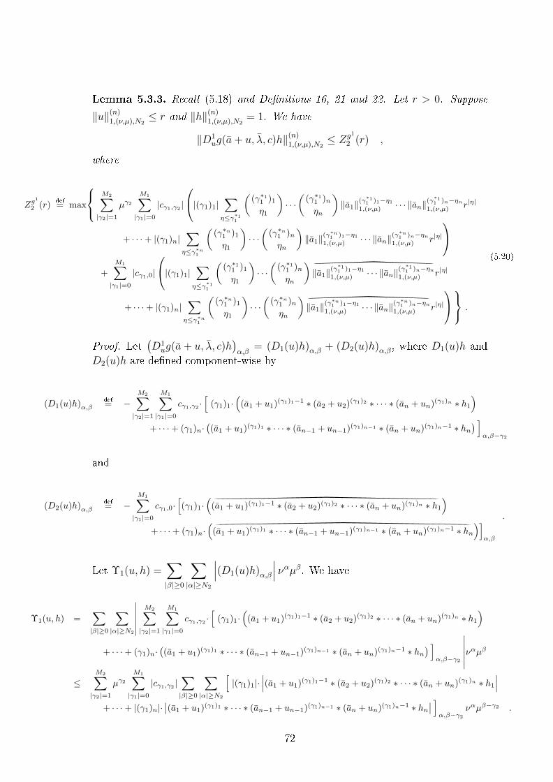
Lemma 5.3.3. Recall (5.18) and De�nitions 16, 21 and 22. Let r > 0. Suppose

‖u‖(n)1,(ν,µ),N2

≤ r and ‖h‖(n)1,(ν,µ),N2

= 1. We have

‖D1ug(a+ u, λ, c)h‖(n)

1,(ν,µ),N2≤ Zg1

2 (r) ,

where

Zg1

2 (r)def

= max

M2∑|γ2|=1

µγ2M1∑|γ1|=0

|cγ1,γ2 |

|(γ1)1|∑η≤γ∗11

((γ∗11 )1η1

)· · ·(

(γ∗11 )nηn

)‖a1‖(γ

∗11 )1−η1

1,(ν,µ) · · · ‖an‖(γ∗11 )n−ηn

1,(ν,µ) r|η|

+ · · ·+ |(γ1)n|∑η≤γ∗n1

((γ∗n1 )1η1

)· · ·(

(γ∗n1 )nηn

)‖a1‖(γ

∗n1 )1−η1

1,(ν,µ) · · · ‖an‖(γ∗n1 )n−ηn

1,(ν,µ) r|η|

+

M1∑|γ1|=0

|cγ1,0|

|(γ1)1|∑η≤γ∗11

((γ∗11 )1η1

)· · ·(

(γ∗11 )nηn

)‖a1‖(γ

∗11 )1−η1

1,(ν,µ) · · · ‖an‖(γ∗11 )n−ηn

1,(ν,µ) r|η|

+ · · ·+ |(γ1)n|∑η≤γ∗n1

((γ∗n1 )1η1

)· · ·(

(γ∗n1 )nηn

)‖a1‖(γ

∗n1 )1−η1

1,(ν,µ) · · · ‖an‖(γ∗n1 )n−ηn

1,(ν,µ) r|η|

.

(5.20)

Proof. Let(D1ug(a+ u, λ, c)h

)α,β

= (D1(u)h)α,β + (D2(u)h)α,β, where D1(u)h and

D2(u)h are de�ned component-wise by

(D1(u)h)α,βdef

= −M2∑|γ2|=1

M1∑|γ1|=0

cγ1,γ2 ·[

(γ1)1·(

(a1 + u1)(γ1)1−1 ∗ (a2 + u2)(γ1)2 ∗ · · · ∗ (an + un)(γ1)n ∗ h1)

+ · · ·+ (γ1)n·((a1 + u1)(γ1)1 ∗ · · · ∗ (an−1 + un−1)(γ1)n−1 ∗ (an + un)(γ1)n−1 ∗ hn

) ]α,β−γ2

and

(D2(u)h)α,βdef

= −M1∑|γ1|=0

cγ1,0·[(γ1)1·

((a1 + u1)(γ1)1−1 ∗ (a2 + u2)(γ1)2 ∗ · · · ∗ (an + un)(γ1)n ∗ h1)

+ · · ·+ (γ1)n·(

(a1 + u1)(γ1)1 ∗ · · · ∗ (an−1 + un−1)(γ1)n−1 ∗ (an + un)(γ1)n−1 ∗ hn)]α,β

.

Let Υ1(u, h) =∑|β|≥0

∑|α|≥N2

∣∣∣(D1(u)h)α,β

∣∣∣ ναµβ. We have

Υ1(u, h) =∑|β|≥0

∑|α|≥N2

∣∣∣∣∣∣M2∑|γ2|=1

M1∑|γ1|=0

cγ1,γ2 ·[

(γ1)1·(

(a1 + u1)(γ1)1−1 ∗ (a2 + u2)(γ1)2 ∗ · · · ∗ (an + un)(γ1)n ∗ h1)

+ · · ·+ (γ1)n·((a1 + u1)(γ1)1 ∗ · · · ∗ (an−1 + un−1)(γ1)n−1 ∗ (an + un)(γ1)n−1 ∗ hn

) ]α,β−γ2

∣∣∣∣∣∣ναµβ≤

M2∑|γ2|=1

µγ2M1∑|γ1|=0

|cγ1,γ2 |∑|β|≥0

∑|α|≥N2

[|(γ1)1|·

∣∣∣(a1 + u1)(γ1)1−1 ∗ (a2 + u2)(γ1)2 ∗ · · · ∗ (an + un)(γ1)n ∗ h1∣∣∣

+ · · ·+ |(γ1)n|·∣∣(a1 + u1)(γ1)1 ∗ · · · ∗ (an−1 + un−1)(γ1)n−1 ∗ (an + un)(γ1)n−1 ∗ hn

∣∣ ]α,β−γ2

ναµβ−γ2 .

72

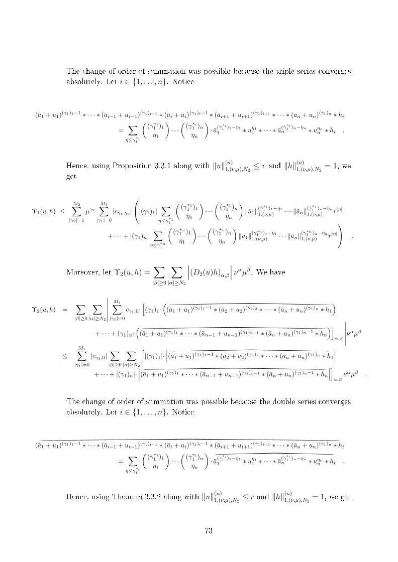
The change of order of summation was possible because the triple series converges

absolutely. Let i ∈ {1, . . . , n}. Notice

(a1 + u1)(γ1)1−1 ∗ · · · ∗ (ai−1 + ui−1)(γ1)i−1 ∗ (ai + ui)(γ1)i−1 ∗ (ai+1 + ui+1)(γ1)i+1 ∗ · · · ∗ (an + un)(γ1)n ∗ hi

=∑η≤γ∗i1

((γ∗i1 )1η1

)· · ·(

(γ∗i1 )nηn

)· a(γ

∗i1 )1−η1

1 ∗ uη11 ∗ · · · ∗ a(γ∗i1 )n−ηn

n ∗ uηnn ∗ hi .

Hence, using Proposition 3.3.1 along with ‖u‖(n)1,(ν,µ),N2

≤ r and ‖h‖(n)1,(ν,µ),N2

= 1, we

get

Υ1(u, h) ≤M2∑|γ2|=1

µγ2M1∑|γ1|=0

|cγ1,γ2 |

|(γ1)1|∑η≤γ∗11

((γ∗11 )1η1

)· · ·(

(γ∗11 )nηn

)‖a1‖(γ

∗11 )1−η1

1,(ν,µ) · · · ‖an‖(γ∗11 )n−ηn

1,(ν,µ) r|η|

+ · · ·+ |(γ1)n|∑η≤γ∗n1

((γ∗n1 )1η1

)· · ·(

(γ∗n1 )nηn

)‖a1‖(γ

∗n1 )1−η1

1,(ν,µ) · · · ‖an‖(γ∗n1 )n−ηn

1,(ν,µ) r|η|

.

Moreover, let Υ2(u, h) =∑|β|≥0

∑|α|≥N2

∣∣∣(D2(u)h)α,β

∣∣∣ ναµβ. We have

Υ2(u, h) =∑|β|≥0

∑|α|≥N2

∣∣∣∣∣∣M1∑|γ1|=0

cγ1,0·[(γ1)1·

((a1 + u1)(γ1)1−1 ∗ (a2 + u2)(γ1)2 ∗ · · · ∗ (an + un)(γ1)n ∗ h1)

+ · · ·+ (γ1)n·(

(a1 + u1)(γ1)1 ∗ · · · ∗ (an−1 + un−1)(γ1)n−1 ∗ (an + un)(γ1)n−1 ∗ hn)]α,β

∣∣∣∣∣∣ναµβ≤

M1∑|γ1|=0

|cγ1,0|∑|β|≥0

∑|α|≥N2

[|(γ1)1|·

∣∣∣(a1 + u1)(γ1)1−1 ∗ (a2 + u2)(γ1)2 ∗ · · · ∗ (an + un)(γ1)n ∗ h1∣∣∣+ · · ·+ |(γ1)n|·

∣∣∣(a1 + u1)(γ1)1 ∗ · · · ∗ (an−1 + un−1)(γ1)n−1 ∗ (an + un)(γ1)n−1 ∗ hn∣∣∣]α,β

ναµβ .

The change of order of summation was possible because the double series converges

absolutely. Let i ∈ {1, . . . , n}. Notice

(a1 + u1)(γ1)1−1 ∗ · · · ∗ (ai−1 + ui−1)(γ1)i−1 ∗ (ai + ui)(γ1)i−1 ∗ (ai+1 + ui+1)(γ1)i+1 ∗ · · · ∗ (an + un)(γ1)n ∗ hi

=∑η≤γ∗i1

((γ∗i1 )1η1

)· · ·(

(γ∗i1 )nηn

)· a(γ

∗i1 )1−η1

1 ∗ uη11 ∗ · · · ∗ a(γ∗i1 )n−ηn

n ∗ uηnn ∗ hi .

Hence, using Theorem 3.3.2 along with ‖u‖(n)1,(ν,µ),N2

≤ r and ‖h‖(n)1,(ν,µ),N2

= 1, we get

73

Υ2(u, h) ≤M1∑|γ1|=0

|cγ1,0|

|(γ1)1|∑η≤γ∗11

((γ∗11 )1η1

)· · ·(

(γ∗11 )nηn

)‖a1‖(γ

∗11 )1−η1

1,(ν,µ) · · · ‖an‖(γ∗11 )n−ηn

1,(ν,µ) r|η|

+ · · ·+ |(γ1)n|∑η≤γ∗n1

((γ∗n1 )1η1

)· · ·(

(γ∗n1 )nηn

)‖a1‖(γ

∗n1 )1−η1

1,(ν,µ) · · · ‖an‖(γ∗n1 )n−ηn

1,(ν,µ) r|η|

.

Finally, the result follows from

‖D1ug(a+ u, c)h‖(n)

1,(ν,µ),N2≤ max

{Υ1(u, h) + Υ2(u, h)

}= Zg1

2 (r) .

The �rst lemma being stated and proved, let us move on to the second one.

Lemma 5.3.4. Recall (5.18) and De�nitions 16, 21 and 22. Let r > 0. Suppose

‖u‖(n)1,(ν,µ),N2

≤ r and ‖h‖(n)1,(ν,µ),N2

= 1. Let h∗ ∈(`1,N2ν,µ

)nbe de�ned component-wise

by

(h∗)α,βdef

=

0 , if |α| ≤ N2 − 1

1|α| ·hα,β , if |α| ≥ N2

.

Then, we have

‖D2ug(a+ u, λ, c)h∗‖(n)

1,(ν,µ),N2≤ Zg2

2 (r) ,

where

Zg2

2 (r)def

= 2·(‖λ1‖1,µ + · · ·+ ‖λk‖1,µ

). (5.21)

Proof. Let Υ(u, h) =∑|β|≥0

∑|α|≥N2

∣∣∣(D2ug(a+ u, λ, c)h∗

)α,β

∣∣∣ ναµβ. We have

Υ(u, h) =∑|β|≥0

∑|α|≥N2

∣∣∣∣((α· λ)∗(h∗)α)β

+ (1− δβ,0)· (α· λ)β· (h∗)α,0∣∣∣∣ ναµβ

=∑|β|≥0

∑|α|≥N2

∣∣∣∣∣(

(α· λ)∗(

1

|α|hα))

β

+ (1− δβ,0)· (α· λ)β·(

1

|α|hα,0)∣∣∣∣∣ ναµβ

≤∑|β|≥0

∑|α|≥N2

[((α· |λ|)∗

(1

|α| |hα|))

β

+ (1− δβ,0)· (α· |λ|)β·(

1

|α| |hα,0|)]

ναµβ

≤∑|β|≥0

∑|α|≥N2

k∑i=1

[(|λi|∗|hα|

)β

+ (1− δβ,0)· (|λi|)β· |hα,0|]ναµβ

74

Let λ(ν,µ)i be de�ned component-wise by

(λ

(ν,µ)i

)α,β

def

=

(λi)β

, if |α| = 0

0 , if |α| 6= 0(i ∈ {1, . . . , k}) .

Notice λ(ν,µ)i ∈

(`1,N2ν,µ

)nfor all i ∈ {1, . . . , k}. Hence,

Υ(u, h) ≤∑|β|≥0

∑|α|≥N2

k∑i=1

[(|λ(ν,µ)i |∗|h|

)α,β

+ (1− δβ,0)·(|λi|)β· (|h|)α,0

]ναµβ .

Let 1def

= (1, . . . , 1) ∈ Rn. Therefore, since ‖h‖(n)1,(ν,µ),N2

= 1 and ‖λ(ν,µ)i ‖1,(ν,µ) =

‖λi‖1,µ (∀i ∈ {1, . . . , k}) � one can verify the latter is indeed true �, we get

Υ(u, h) ≤k∑i=1

1·[‖λi‖1,µ + ‖λi‖1,µ

]

= 2k∑i=1

1· ‖λi‖1,µ .

Finally, the result follows from

‖D2ug(a+ u, λ, c)h∗‖(n)

1,(ν,µ),N2≤ max

{Υ(u, h)

}≤ Zg2

2 (r) .

We can now apply the Radii Polynomials Approach (see Subsection 3.4) one last

time to see what are the conditions needed for the operator T2 :(`1,N2ν,µ

)n → (`1,N2ν,µ

)ngiven by (4.14) to have a �xed point close to u = 0.

Theorem 5.3.3. Recall T2 :(`1,N2ν,µ

)n → (`1,N2ν,µ

)n, the operator given by (4.15). Let

K1def

=10

9·N2·min{∣∣λ0

∣∣}· ‖P−1‖∞· ‖P‖∞ & K2def

=10

9·min{∣∣λ0

∣∣}· ‖P−1‖∞· ‖P‖∞ .

Recall the bounds (Y2)0, Zg1

2 (r) and Zg2

2 (r) de�ned in (5.19), (5.20) and (5.21) re-spectively. Let

Z1def

= K1·max

M2∑|γ2|=1

µγ2M1∑|γ1|=0

|cγ1,γ2 |(|(γ1)1|· ‖a1‖(γ

∗11 )1

1,(ν,µ) · · · ‖an‖(γ∗11 )n

1,(ν,µ) + · · ·+ |(γ1)n|· ‖a1‖(γ∗n1 )1

1,(ν,µ) · · · ‖an‖(γ∗n1 )n1,(ν,µ)

)

+

M1∑|γ1|=0

|cγ1,0|(|(γ1)1|· ‖a1‖(γ

∗11 )1

1,(ν,µ) · · · ‖an‖(γ∗11 )n

1,(ν,µ) + · · ·+ |(γ1)n|· ‖a1‖(γ∗n1 )1

1,(ν,µ) · · · ‖an‖(γ∗n1 )n1,(ν,µ)

)+K2·Zg

2

2 (r)

(5.22)

75

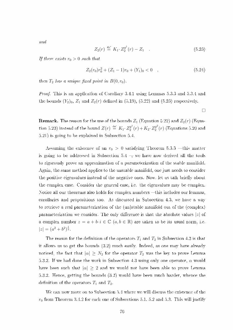
and

Z2(r)def

= K1·Zg1

2 (r)− Z1 . (5.23)

If there exists r0 > 0 such that

Z2(r0)r20 + (Z1 − 1)r0 + (Y1)0 < 0 , (5.24)

then T2 has a unique �xed point in B(0, r0).

Proof. This is an application of Corollary 3.4.1 using Lemmas 5.3.3 and 5.3.4 and

the bounds (Y2)0, Z1 and Z2(r) de�ned in (5.19), (5.22) and (5.23) respectively.

Remark. The reason for the use of the bounds Z1 (Equation 5.22) and Z2(r) (Equa-

tion 5.23) instead of the bound Z(r)def

= K1·Zg1

2 (r)+K2·Zg2

2 (r) (Equations 5.20 and

5.21) is going to be explained in Subsection 5.4.

Assuming the existence of an r0 > 0 satisfying Theorem 5.3.3 � this matter

is going to be addressed in Subsection 5.4 �, we have now derived all the tools

to rigorously prove an approximation of a parameterization of the stable manifold.

Again, the same method applies to the unstable manifold, one just needs to consider

the positive eigenvalues instead of the negative ones. Now, let us talk brie�y about

the complex case. Consider the general case, i.e. the eigenvalues may be complex.

Notice all our theorems also holds for complex numbers � this includes our lemmas,

corollaries and propositions too. As discussed in Subsection 4.3, we have a way

to retrieve a real parameterization of the (un)stable manifold out of the (complex)

parameterization we consider. The only di�erence is that the absolute values |z| ofa complex number z = a + b· i ∈ C (a, b ∈ R) are taken to be its usual norm, i.e.

|z| = (a2 + b2)12 .

The reason for the de�nition of the operators T1 and T2 in Subsection 4.3 is that

it allows us to get the bounds (3.2) much easily. Indeed, as one may have already

noticed, the fact that |α| ≥ N2 for the operator T2 was the key to prove Lemma

5.3.2. If we had done the work in Subsection 4.3 using only one operator, α would

have been such that |α| ≥ 2 and we would not have been able to prove Lemma

5.3.2. Hence, getting the bounds (3.2) would have been much harder, whence the

de�nition of the operators T1 and T2.

We can now move on to Subsection 5.4 where we will discuss the existence of the

r0 from Theorem 3.4.2 for each one of Subsections 5.1, 5.2 and 5.3. This will justify

76

the usefulness of the Parameterization method (see Subsection 2.3) we introduced

in this thesis.

5.4 Control of the error via Radii Polynomials

Recall Theorems 5.1.1, 5.2.1, 5.3.1 and 5.3.3. Consider Equations 5.6, 5.12,

5.17 and 5.24. Notice each of their left hand side member is a polynomial in r.

Hence, trying to get the existence of an r0 > 0 such that those polynomials are

negative � this r0 need not be the same for each of those polynomials � boils down

to solving for the roots of those polynomials. Indeed, a positive root for one of

them implies the existence of a desired r0 > 0 for it by continuity � we disregard

the case of multiple roots because one only needs to diminish the weight(s) to get

a lower Y0 bound while keeping the previous values for the other bounds. Since all

the bounds derived in Subsections 5.1, 5.2 and 5.3 are nonnegative, the only way

for those polynomials to have a positive root is to have a negative coe�cient for

their �rst order term. This coe�cient has the same form for all four polynomials.

Without loss of generality, say it is Z − 1. Notice that, for all four polynomials, Z

does not depend on r. Moreover, each member of Z depends on the weight(s) of the

Banach space considered (see De�nition 13). Hence, we can make Z as small as we

want by taking the weight(s) as small as needed. Therefore, we can ensure Z to be

less than 1, i.e. Z − 1 to be negative. Finally, we can always ensure the existence of

a positive root for each four polynomials by taking the bounds as small as needed �

we can always do so because each member of the bounds depends on the weight(s).

Let us talk about our approximations being "good enough". Let S be any of the

series we considered. Let S be the approximation of S we considered. The weight

of the Banach space considered for its proof is less than the radius of convergence

of S. Moreover, the distance between S and S � the distance is taken using the

norm of the Banach space considered � is at most r0 > 0 � it exists by the above

discussion. Since Y0 can be taken very small by diminishing the weight of the Banach

space considered, r0 > 0 can be taken as small as we want. A dilemma arises here

: A better approximation � this means a lesser r0 � is taken at the cost of a lesser

radius of convergence of S. Nevertheless, we will see in Section 7 that, depending

on the purpose of the parameterization of the (un)stable manifold, one can choose

the better approximation over the radius of convergence.

Let us now talk about the propagation of the error throughout the computations.

77

As mentioned above, the distance between S and S is r0. Let sδ and sδ be the

coe�cients at index δ of the power series S and S respectively. Let υ be the weight

considered for the validation of S. We have

maxi∈{1,...,n}

|(si)δ − (si)δ| <r0

υδ(∀δ) .

Hence, we know that

(si)δ ∈(

(si)δ −r0

υδ, (si)δ +

r0

υδ

)(∀i ∈ {1, . . . , n},∀δ) .

Therefore, we can use this interval in our computations to keep track of the error.

The computations can then be done using the Interval arithmetic (see [21]) for

the sake of completeness. This ensures the results include the errors on all the

approximations. A direct consequence of the Interval arithmetic is that the r0 from

Theorem 3.4.2 may be bigger than intended � this is still acceptable � or negative

� this would require a better job at getting the bounds (3.2), namely diminishing

the weight(s). Nonetheless, as shown in this section, we can guarantee the existence

of r0 for Theorems 5.1.1, 5.2.1, 5.3.1 and 5.3.3, so it is not mandatory to use the

Interval arithmetic.

As discussed above, given Assumptions A1, A2, A3 and A4, our method allows

to retrieve rigorously � this is because we can always guarantee the existence of r0 �

and e�ciently � this is because the recurrence relations only involve basic operations

� a parameterization of the (un)stable manifold. We are now ready to go over two

examples to see what the method looks like in practice.

78

6 Applications

We are going to go over two examples (Subsections 6.1 and 6.2) to see how the

computations look like in practice. In sections 4 and 5, we considered Assumption

A2, i.e. the vector �eld is polynomial. This implied considering all the terms of

the polynomial vector �eld up to its order � the order was M1 in space and M2 in

parameters in our settings (see Equation 4.1). Nonetheless, in practice, one often

has only a couple of terms. This makes the computations much easier in the sense

that there are fewer of them.

For Subsections 6.1 and 6.2, we are only going to state the operators and their

derivative, as well as the bounds (3.2) used for the theorems we derived in Section 5

to validate our computations. We refer the reader to Sections 4 and 5 for the proofs.

6.1 Lorenz system

Let us start with a famous example : The Lorenz system (see [20]). In the

Lorenz system (LS), the vector �eld f : R3 → R3 is given by

f(x, y, z)def

=

σ(y − x)

(ρ− z)x− yxy − βz

where σ, ρ, β ∈ R are parameters that will be �xed. Let us introduce another

parameter in it, say ω ∈ R. We will consider the new vector �eld f : R3 × R→ R3

given by

f(x, ω)def

=

σp(x2 − x1)

(ρp + ω − x3)x1 − x2

x1x2 − βpx3

(6.1)

where (σp, ρp, βp) = (10, 28, 8/3) � we use the notation (σp, ρp, βp) instead of (σ, ρ, β)

to avoid confusion between the parameter β and the index β. One can verify that

x0def

= (0, 0, 0) is a �xed point of (6.1) for ω = 0. Recall Section 4. We need to

compute the �xed point along with its associated eigenvalues and eigenvectors with

respect to the parameter ω in order to get to the computation of the parameterization

of the (un)stable manifold at each of them. We are going to consider the value ω = 0

of ω. Assumptions A1 and A3 will be veri�ed for ω = 0 and the aforementioned

�xed point, as well as Assumption A4. Notice that Assumption A2 is veri�ed

because the vector �eld de�ned in (6.1) is polynomial.

79

Let us move on to the computation of a parameterization of the (un)stable man-

ifold in a neighbourhood of the �xed point x0 and ω = ω.

6.1.1 Fixed point (LS)

We start with the computation of the �xed point. Recall the recurrence

relation onto the coe�cients of x(ω) is given by Equation 4.4. Thereby, for β ≥ 1,

we have

−σp σp 0

ρp − (b3)0 −1 −(b1)0

(b2)0 (b1)0 −βp

︸ ︷︷ ︸

B

bβ =

0

−(b1)β−1 + (b1∗b3)β

−(b1∗b2)β

.

SinceDxf(x(ω), ω) = B has no purely imaginary eigenvalues for x(ω) = x0 � one can

verify the latter is indeed true �, x(ω) is an hyperbolic �xed point, so Assumption

A1 is veri�ed.

Recall Theorem 5.1.1. Using the bounds Y0, Z1 and Z2(r), respectively de�ned

in (5.2), (5.4) and (5.5), we numerically get the results of Table 1. Hence, using the

x0

µ = 0.9 & N = 12

Y0 0

Z1 0.3375

Z2(r) 0.75r

r0 [0, 0.883]

Table 1 � Lorenz Fixed Point Results

data from Table 1, Theorem 5.1.1 validates our approximation b of the coe�cients

of the power series of x(ω).

Let us now move on to the computation of the eigenvalues and their associated

eigenvector.

80

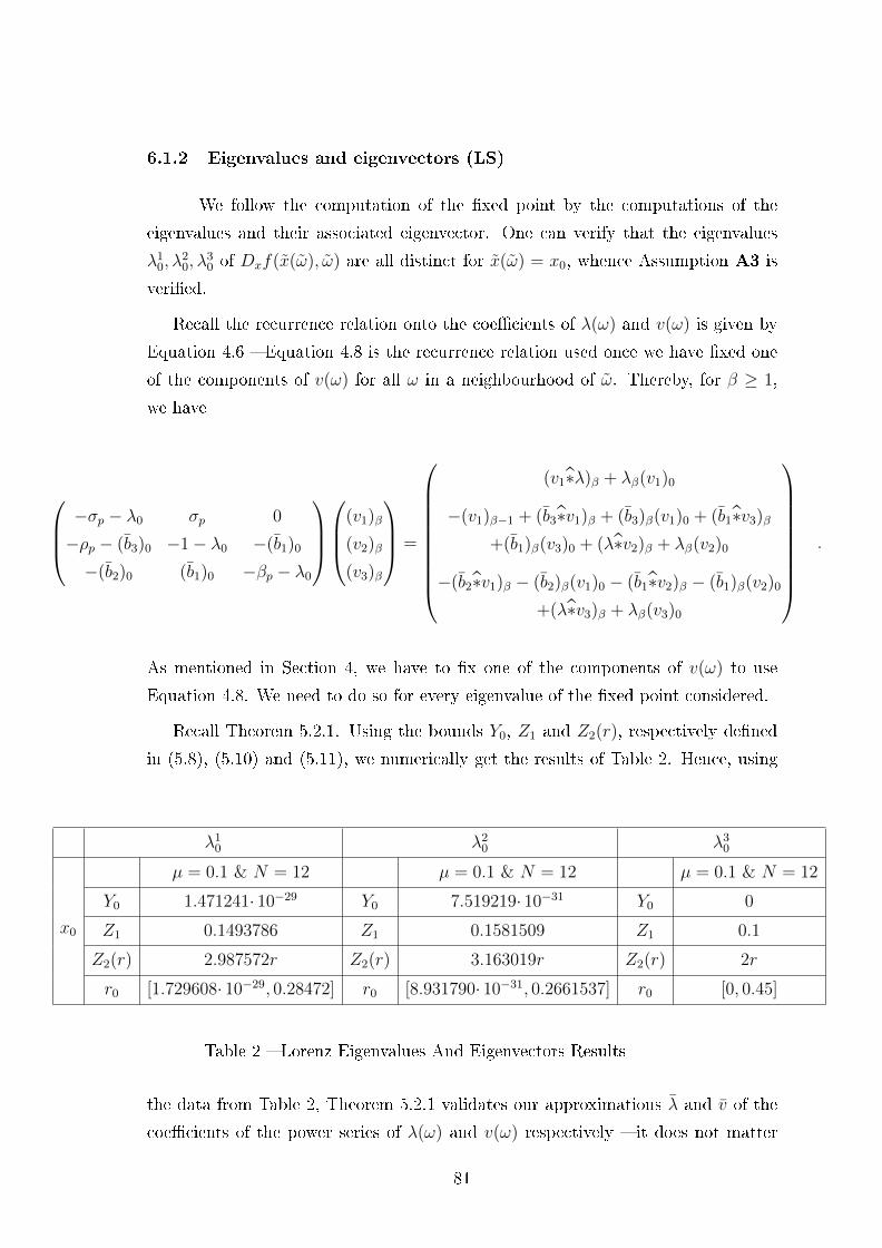
6.1.2 Eigenvalues and eigenvectors (LS)

We follow the computation of the �xed point by the computations of the

eigenvalues and their associated eigenvector. One can verify that the eigenvalues

λ10, λ

20, λ

30 of Dxf(x(ω), ω) are all distinct for x(ω) = x0, whence Assumption A3 is

veri�ed.

Recall the recurrence relation onto the coe�cients of λ(ω) and v(ω) is given by

Equation 4.6 � Equation 4.8 is the recurrence relation used once we have �xed one

of the components of v(ω) for all ω in a neighbourhood of ω. Thereby, for β ≥ 1,

we have

−σp − λ0 σp 0

−ρp − (b3)0 −1− λ0 −(b1)0

−(b2)0 (b1)0 −βp − λ0

(v1)β

(v2)β

(v3)β

=

(v1∗λ)β + λβ(v1)0

−(v1)β−1 + (b3∗v1)β + (b3)β(v1)0 + (b1∗v3)β

+(b1)β(v3)0 + (λ∗v2)β + λβ(v2)0

−(b2∗v1)β − (b2)β(v1)0 − (b1∗v2)β − (b1)β(v2)0

+(λ∗v3)β + λβ(v3)0

.

As mentioned in Section 4, we have to �x one of the components of v(ω) to use

Equation 4.8. We need to do so for every eigenvalue of the �xed point considered.

Recall Theorem 5.2.1. Using the bounds Y0, Z1 and Z2(r), respectively de�ned

in (5.8), (5.10) and (5.11), we numerically get the results of Table 2. Hence, using

λ10 λ2

0 λ30

x0

µ = 0.1 & N = 12 µ = 0.1 & N = 12 µ = 0.1 & N = 12

Y0 1.471241· 10−29 Y0 7.519219· 10−31 Y0 0

Z1 0.1493786 Z1 0.1581509 Z1 0.1

Z2(r) 2.987572r Z2(r) 3.163019r Z2(r) 2r

r0 [1.729608· 10−29, 0.28472] r0 [8.931790· 10−31, 0.2661537] r0 [0, 0.45]

Table 2 � Lorenz Eigenvalues And Eigenvectors Results

the data from Table 2, Theorem 5.2.1 validates our approximations λ and v of the

coe�cients of the power series of λ(ω) and v(ω) respectively � it does not matter

81

which eigenvalues of Dxf(x(ω), ω) are λ10, λ

20 and λ

30 because we can pick any r0 that

veri�es Equation 5.12 for all of them. Note that we need to repeat this procedure

for every eigenvalue of Dxf(x(ω), ω) and their associated eigenvector.

Let us now move on to the computation of the parameterization of the (un)stable

manifold.

6.1.3 Stable and unstable manifolds coe�cients (LS)

We follow the computations of the eigenvalues and their associated eigenvec-

tor by the computation of a parameterization of the (un)stable manifold. Recall

De�nition 18. One can verify that Dxf(x(ω), ω) has no resonance for x(ω) = x0,

whence Assumption A4 is veri�ed.

Recall the recurrence relation onto the coe�cients of P (θ, ω) is given by Equation

4.13. Thereby, for |α| ≥ 2, we have

aα,β = B−1α

0

−(a1)α,β−1 + (a1∗a3)α,β

−(a1∗a2)α,β

+(

(α·λ)∗aα)β

+ (1− δβ,0)· (α·λ)βaα,0

where

Bα =

−σp − (α· λ)0 σp 0

ρp − (a3)0,0 −1− (α· λ)0 −(a1)0,0

(a2)0,0 (a1)0,0 −βp − (α· λ)0

.

Recall Theorem 5.3.1. Let P s = P s(θ, ω) and P u = P u(θ, ω) respectively be the

parameterizations of the stable and unstable manifolds at x(ω). Using the bounds

(Y1)0 and Z1(r), respectively de�ned in (5.14) and (5.16), we numerically get the

results of Table 3. For the sake of simplicity, Table 3 only displays the results of the α

for which the interval containing r0 has the highest lower bound. Notice this interval

is contained in the ones from the other values of α up to order N2− 1 (see Table 4).

Hence, using the data from Table 3, Theorem 5.3.1 validates our approximation aα

of the coe�cients of the power series of P (θ, ω) for α �xed up to order N2− 1 � the

notation P (θ, ω) is used for both P s and P u.

82

P s P u

x0

µ = 0.01 & N1 = 12 µ0.1 = & N1 = 12

α [1 1] α 2

(Y1)0 3.162076· 10−43 (Y1)0 2.220395· 10−33

Z1 0.005632 Z1 0.017691

r0 [3.179983· 10−43,∞) r0 [2.260385· 10−33,∞)

Table 3 � Lorenz Stable And Unstable Manifolds Results for α �xed

Finally, recall Theorem 5.3.3. Using the bounds (Y2)0, Z1 and Z2(r), respectively

de�ned in (5.19), (5.22) and (5.23), we numerically get the results of Table 4. Hence,

P s P u

x0

ν = [0.1 0.1]

& µ = 0.01 & N2 = 8

ν = 1

& µ = 0.1 & N2 = 11

(Y2)0 7.315016· 10−16 (Y2)0 3.048495· 10−17

Z1 0.353093 Z1 0.040743

Z2(r) 0.319654r Z2(r) 0.050449r

r0 [1.130768· 10−15, 2.023774] r0 [3.177974· 10−17, 19.0147]

Table 4 � Lorenz Stable And Unstable Manifolds Results

using the data from Table 4, Theorem 5.3.3 validates our approximation a of the

coe�cients of the power series of P (θ, ω) � the notation P (θ, ω) is again used for

both P s and P u.

Figures 9 and 11 respectively show our approximations of the stable and unstable

manifolds at x(ω) = x0. Figures 10 and 12 respectively show a globalization of the

stable and unstable manifolds at x(ω) = x0 we computed. The globalizations are

done using the ode45 function in MATLAB. The red dot is the origin. The Lorenz

attractor (see [20]) was highlighted in green in Figure 10.

Let us now move on to an example in higher dimensions.

83

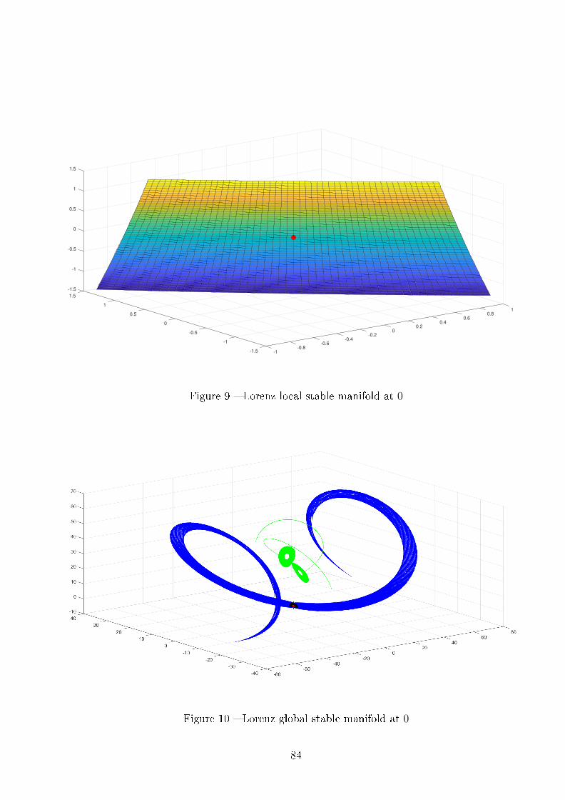
-1.5

1.5

-1

1

-0.5

1

0

0.80.50.6

0.5

0.40

1

0.20

1.5

-0.5-0.2

-0.4-1 -0.6

-0.8-1.5 -1

Figure 9 � Lorenz local stable manifold at 0

Figure 10 � Lorenz global stable manifold at 0

84

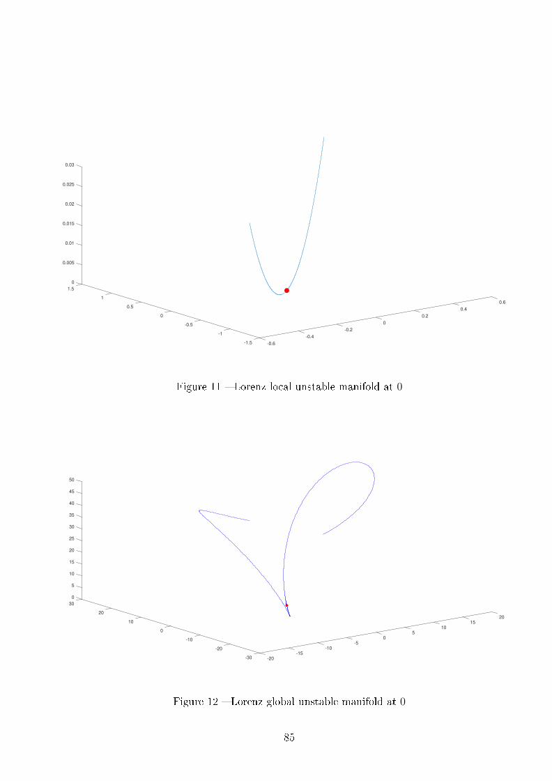
0

1.5

0.005

1

0.01

0.6

0.015

0.50.4

0.02

0 0.2

0.025

0

0.03

-0.5

-0.2-1

-0.4

-1.5 -0.6

Figure 11 � Lorenz local unstable manifold at 0

0

30

5

10

15

20

20

20

25

10 15

30

10

35

0

40

5

45

0

50

-10-5

-10-20

-15-30 -20

Figure 12 � Lorenz global unstable manifold at 0

85

6.2 Rolls and Hexagons system

Let us continue with another example : The Rolls and Hexagons system (RH)

from [3]. In this system, the vector �eld Ψ : R4 × R→ R4 is given by

Ψ(U, c) =

U2

−14cβU2 − γ

4U1 −

√2

4U2

3 + 38U3

1 + 3U1U23

U4

− cβU4 − γU3 −

√2

2U1U3 + 9U3

3 + 3U21U3

where γ, β ∈ R are parameters that will be �xed. Let us rewrite it using our notation,

i.e. consider the vector �eld f : R4 × R→ R4 given by

f(x, ω)def

=

x2

−14ωβpx2 − γp

4x1 −

√2

4x2

3 + 38x3

1 + 3x1x23

x4

− ωβpx4 − γpx3 −

√2

2x1x3 + 9x3

3 + 3x21x3

(6.2)

where (γp, βp) =((7 + 3

√6)/30, 1

)� we use the notation (γp, βp) instead of (γ, β)

to avoid confusion between the parameter β and the index β as well as between the

parameter γ and the index γ. One can verify that x0def

= (−√

2γp/3, 0, 0, 0) is a �xed

point of (6.2) for ω = 0. Recall Section 4. We need to compute this �xed point along

with its associated eigenvalues and eigenvectors with respect to the parameter ω in

order to get to the computation of the parameterization of the (un)stable manifold

at it. We are going to consider the value ω = 0 of ω. Assumptions A1 and A3

will be veri�ed for ω = 0 and the aforementioned �xed point, as well as Assumption

A4. Notice that Assumption A2 is veri�ed because the vector �eld de�ned in (6.2)

is polynomial.

Let us move on to the computation of a parameterization of the (un)stable man-

ifold in a neighbourhood of x0 and ω = ω.

86

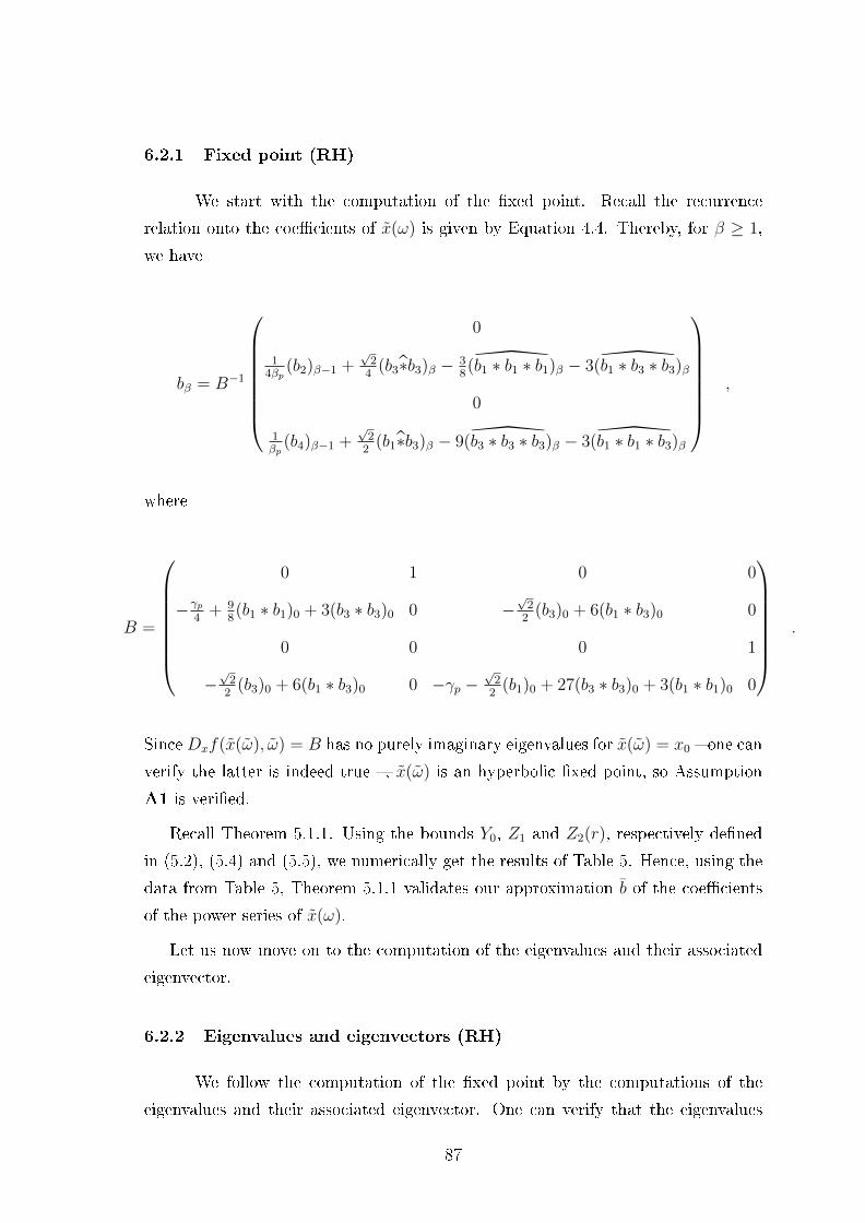
6.2.1 Fixed point (RH)

We start with the computation of the �xed point. Recall the recurrence

relation onto the coe�cients of x(ω) is given by Equation 4.4. Thereby, for β ≥ 1,

we have

bβ = B−1

0

14βp

(b2)β−1 +√

24

(b3∗b3)β − 38(b1 ∗ b1 ∗ b1)β − 3(b1 ∗ b3 ∗ b3)β

0

1βp

(b4)β−1 +√

22

(b1∗b3)β − 9(b3 ∗ b3 ∗ b3)β − 3(b1 ∗ b1 ∗ b3)β

,

where

B =

0 1 0 0

−γp4

+ 98(b1 ∗ b1)0 + 3(b3 ∗ b3)0 0 −

√2

2(b3)0 + 6(b1 ∗ b3)0 0

0 0 0 1

−√

22

(b3)0 + 6(b1 ∗ b3)0 0 −γp −√

22

(b1)0 + 27(b3 ∗ b3)0 + 3(b1 ∗ b1)0 0

.

SinceDxf(x(ω), ω) = B has no purely imaginary eigenvalues for x(ω) = x0 � one can

verify the latter is indeed true �, x(ω) is an hyperbolic �xed point, so Assumption

A1 is veri�ed.

Recall Theorem 5.1.1. Using the bounds Y0, Z1 and Z2(r), respectively de�ned

in (5.2), (5.4) and (5.5), we numerically get the results of Table 5. Hence, using the

data from Table 5, Theorem 5.1.1 validates our approximation b of the coe�cients

of the power series of x(ω).

Let us now move on to the computation of the eigenvalues and their associated

eigenvector.

6.2.2 Eigenvalues and eigenvectors (RH)

We follow the computation of the �xed point by the computations of the

eigenvalues and their associated eigenvector. One can verify that the eigenvalues

87

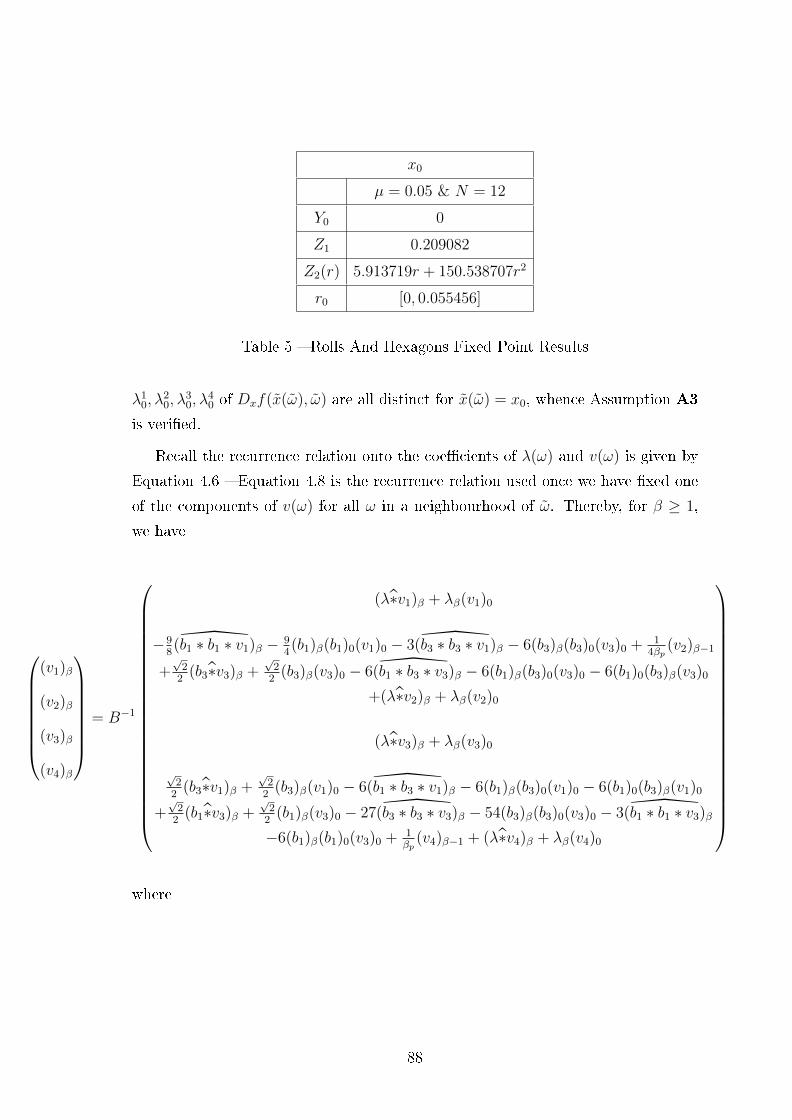
x0

µ = 0.05 & N = 12

Y0 0

Z1 0.209082

Z2(r) 5.913719r + 150.538707r2

r0 [0, 0.055456]

Table 5 � Rolls And Hexagons Fixed Point Results

λ10, λ

20, λ

30, λ

40 of Dxf(x(ω), ω) are all distinct for x(ω) = x0, whence Assumption A3

is veri�ed.

Recall the recurrence relation onto the coe�cients of λ(ω) and v(ω) is given by

Equation 4.6 � Equation 4.8 is the recurrence relation used once we have �xed one

of the components of v(ω) for all ω in a neighbourhood of ω. Thereby, for β ≥ 1,

we have

(v1)β

(v2)β

(v3)β

(v4)β

= B−1

(λ∗v1)β + λβ(v1)0

−98(b1 ∗ b1 ∗ v1)β − 9

4(b1)β(b1)0(v1)0 − 3(b3 ∗ b3 ∗ v1)β − 6(b3)β(b3)0(v3)0 + 1

4βp(v2)β−1

+√

22

(b3∗v3)β +√

22

(b3)β(v3)0 − 6(b1 ∗ b3 ∗ v3)β − 6(b1)β(b3)0(v3)0 − 6(b1)0(b3)β(v3)0

+(λ∗v2)β + λβ(v2)0

(λ∗v3)β + λβ(v3)0

√2

2(b3∗v1)β +

√2

2(b3)β(v1)0 − 6(b1 ∗ b3 ∗ v1)β − 6(b1)β(b3)0(v1)0 − 6(b1)0(b3)β(v1)0

+√

22

(b1∗v3)β +√

22

(b1)β(v3)0 − 27(b3 ∗ b3 ∗ v3)β − 54(b3)β(b3)0(v3)0 − 3(b1 ∗ b1 ∗ v3)β

−6(b1)β(b1)0(v3)0 + 1βp

(v4)β−1 + (λ∗v4)β + λβ(v4)0

where

88

B =

−λ0 1 0 0

−γp4

+ 98(b1 ∗ b1)0 + 3(b3 ∗ b3)0 −λ0 −

√2

2(b3)0 + 6(b1 ∗ b3)0 0

0 0 −λ0 1

−√

22

(b3)0 + 6(b1 ∗ b3)0 0 −γp −√

22

(b1)0 + 27(b3 ∗ b3)0 + 3(b1 ∗ b1)0 −λ0

.

As mentioned in Section 4, we have to �x one of the components of v(ω) to use

Equation 4.8. We need to do so for every eigenvalue of the �xed point considered.

Recall Theorem 5.2.1. Using the bounds Y0, Z1 and Z2(r), respectively de�ned

in (5.8), (5.10) and (5.11), we numerically get the results of Table 6. Hence, using

x0

λ10

µ = 0.1 & N = 12

λ20

µ = 0.1 & N = 12

Y0 1.027719· 10−17 Y0 1.027719· 10−17

Z1 0.572760 Z1 0.572760

Z2(r) 6.067386 Z2(r) 6.067386

r0 [2.405486· 10−17, 0.070416] r0 [2.405486· 10−17, 0.070416]

λ30

µ = 0.1 & N = 12

λ40

µ = 0.1 & N = 12

Y0 7.804082· 10−22 Y0 7.804082· 10−22

Z1 0.26276 Z1 0.26276

Z2(r) 4.66467 Z2(r) 4.66467

r0 [1.058554· 10−21, 0.158048] r0 [1.058554· 10−21, 0.158048]

Table 6 � Lorenz Eigenvalues And Eigenvectors Results

the data from Table 6, Theorem 5.2.1 validates our approximations λ and v of the

coe�cients of the power series of λ(ω) and v(ω) respectively � it does not matter

which eigenvalues of Dxf(x(ω), ω) are λ10, λ

20, λ

30 and λ4

0 because we can pick any

r0 that veri�es Equation 5.12 for all of them. Note that we need to repeat this

procedure for every eigenvalue of Dxf(x(ω), ω) and their associated eigenvector.

Let us now move on to the computation of the parameterization of the (un)stable

manifold.

89

6.2.3 Stable and unstable manifolds coe�cients (RH)

We follow the computations of the eigenvalues and their associated eigenvec-

tor by the computation of a parameterization of the (un)stable manifold. Recall

De�nition 18. One can verify that Dxf(x(ω), ω) has no resonance for x(ω) = x0,

whence Assumption A4 is veri�ed.

Recall the recurrence relation onto the coe�cients of P (θ, ω) is given by Equation

4.13. Thereby, for |α| ≥ 2, we have

aα,β = B−1α

((α·λ)∗(a1)α

)β

+ (1− δβ,0)· (α·λ)β(a1)α,0

14βp

(a2)α,β−1 +√

24

(a3∗a3)α,β − 38(a1 ∗ a1 ∗ a1)α,β − 3(a1 ∗ a3 ∗ a3)α,β

+(

(α·λ)∗(a2)α

)β

+ (1− δβ,0)· (α·λ)β(a2)α,0((α·λ)∗(a3)α

)β

+ (1− δβ,0)· (α·λ)β(a3)α,0

1βp

(a4)α,β−1 +√

22

(a1∗a3)α,β − 9(a3 ∗ a3 ∗ a3)α,β − 3(a1 ∗ a1 ∗ a3)α,β

+(

(α·λ)∗(a4)α

)β

+ (1− δβ,0)· (α·λ)β(a4)α,0

where

Bα =

−(α·λ)0 1 0 0

−γp4

+ 98(a1)2

0,0 + 3(a3)20,0 −(α·λ)0 −

√2

2(a3)0,0 + 6(a1)0,0(a3)0,0 0

0 0 −(α·λ)0 1

−√

22

(a3)0,0 + 6(a1)0,0(a3)0,0 0 −γp −√

22

(a1)0,0 + 27(a3)20,0 + 3(a1)2

0,0 −(α·λ)0

.

Recall Theorem 5.3.1. Let P s = P s(θ, ω) and P u = P u(θ, ω) respectively be the

parameterizations of the stable and unstable manifolds at x(ω). Using the bounds

(Y1)0 and Z1(r), respectively de�ned in (5.14) and (5.16), we numerically get the

results of Table 7. For the sake of simplicity, Table 7 only displays the results of the α

for which the interval containing r0 has the highest lower bound. Notice this interval

is contained in the ones from the other values of α up to order N2− 1 (see Table 8).

Hence, using the data from Table 7, Theorem 5.3.1 validates our approximation aα

90

x0

P s

µ = 10−6 & N1 = 12

P u

µ = 10−6 & N1 = 12

α [1 1] α [1 1]

(Y1)0 0 (Y1)0 0

Z1 3.41188· 10−6 Z1 3.41188· 10−6

r0 [0,∞) r0 [0,∞)

Table 7 � Rolls And Hexagons Stable And Unstable Manifolds Results for α �xed

of the coe�cients of the power series of P (θ, ω) for α �xed up to order N2− 1 � the

notation P (θ, ω) is used for both P s and P u.

Finally, recall Theorem 5.3.3. Using the bounds (Y2)0, Z1 and Z2(r), respectively

de�ned in (5.19), (5.22) and (5.23), we numerically get the results of Table 8. Hence,

x0

P s

ν = (10−3, 10−3)

& µ = 10−6 & N2 = 8

P u

ν = (10−3, 10−3)

& µ = 10−6 & N2 = 8

(Y2)0 3.990597· 10−18 (Y2)0 3.964935· 10−18

Z1 3.928334· 10−3 Z1 3.928334· 10−3

Z2(r) 0.702889r + 16.604092r2 Z2(r) 0.702889r + 16.604092r2

r0 [4.006335· 10−18, 0.224674] r0 [3.980572· 10−18, 0.224674]

Table 8 � Rolls And Hexagons Stable And Unstable Manifolds Results

using the data from Table 8, Theorem 5.3.3 validates our approximation a of the

coe�cients of the power series of P (θ, ω) � the notation P (θ, ω) is again used for

both P s and P u.

We show no �gures for this example because one has to make sense of a 3D or

2D projection of a 4-dimensional problem.

91

92

7 Conclusion

Recall the purpose of this thesis was to develop a rigorous method to compute

stable and unstable manifolds of ODEs satisfying Assumptions A1, A2, A3 and

A4. Section 2 introduced the notion of stable and unstable manifolds of �xed

points depending on parameters. Section 3 went over the necessary tools required to

develop our method. Sections 4 and 5 were the core of the method as it was developed

mainly in these two sections. Finally, Section 6 covered two examples to illustrate

our method. Note we saw in Subsection 5.4 that one can always guarantee the

accuracy of our computations using the Radii Polynomials approach (see Subsection

3.4), thus ensuring the viability of this method.

Even though the work in this thesis has its limits, as it only allows to compute

local parameterizations of stable and unstable manifolds of �xed points, it has several

applications. For instance, one might be interested in the intersection of stable and

unstable manifolds of �xed points. More often than not, the presence of parameters

is needed in order to get such an intersection (see [22]), which is part of the settings of

our method. These intersections are called homoclinic orbits when the �xed points

for both manifolds are the same and heteroclinic orbits otherwise. For example,

in biology, predator-prey models make use of these orbits and have a parameter

dependency (see [15]). Indeed, it is used to predict the evolution of a species as time

goes by. Moreover, in physics, chaos control theory also makes use of these orbits

and requires parameters too (see [9]). Indeed, unusual behaviours, like homoclinic

and heteroclinic orbits, occur for certain values of the parameters.

As mentioned in Section 1, stable and unstable manifolds of �xed points with a

parameter dependency receive a lot of attention nowadays. A follow-up to this thesis

could be the globalization of the local parameterizations of the stable and unstable

manifolds of �xed points with respect to parameters we obtain through our method.

For instance, spacecraft missions make use of these globalizations (see [16]). Indeed,

it allows scientists to move satellites in space using as low fuel as possible for as long

as possible. Therefore, the method developed in this thesis could be adapted to this

end. Moreover, it would provide computations as well as accuracy using the same

ideas as we developed in this thesis.

Finally, the method developed in this thesis could be applied to the computation

of local parameterizations of stable and unstable manifolds of periodic orbits. Those

are more than useful in spacecraft missions and have been used for 20 years (see [12]).

93

Indeed, periodic solutions always show up in spacecraft missions and, as opposed to

�xed point, are lengthy. Therefore, the idea is to send satellites onto those orbits,

using as low fuel as possible, via their stable and unstable manifolds. The same

tools as the ones used in this thesis could be applied to compute those new objects

with the accuracy of our method.

94

Appendix

Theorem A.1 (Implicit Function Theorem). Let W be an open subset of Rm×Rn.

Let f = f(x, y) : W → Rn be continuously di�erentiable over W . Let (a, b) ∈ Wsatisfy

1. f(a, b) = 0 ;

2. f ′(a, b) = (A|B),

where A = ∂f/∂x ∈Mn×m(R) and B = ∂f/∂y ∈Mn×n(R) with B invertible. Then,

there exists neighbourhoods U and V of a and b respectively such that, for all x ∈ U ,there exists a unique y ∈ V satisfying f(x, y) = 0. Moreover, writing y = g(x),

the map g : U → V is continuously di�erentiable over U and satis�es g(a) = b and

g′(a) = −B−1A.

Proof. See [17].

Theorem A.2 (Strong Implicit Function Theorem). Recall Theorem A.1. If the

function f is l times di�erentiable, then so is the function g. Moreover, if the

function f is analytic, then so is the function g.

Proof. See [17].

95

References

[1] Xavier Cabré, Ernest Fontich, Raphael de la Llave. The parameterization method

for invariant manifolds III: Overview and applications. Journal of Di�erential

Equations, 218(2):444-515, 2005.

[2] J. D. Mireles-James. Polynomial approximation of one parameter families of

(un)stable manifolds with rigorous computed assisted error bounds Indagationes

Mathematicae, 26(1), 2014.

[3] Jan Bouwe van den Berg, Andréa Deschênes, Jean-Philippe Lessard, Jason D.

Mireles James. Stationary Coexistence of Hexagons and Rolls via Rigorous Com-

putations. Siam J. Applied Dynamical Systems, 2015.

[4] Lawrence Perko. Di�erential Equations and Dynamical Systems, Third Edition.

Springer, 2001.

[5] Jenny Wilson. Manifolds.

http://www.math.lsa.umich.edu/ jchw/WOMPtalk-Manifolds.pdf

[6] J. Hadamard. Sur l'itération et les solutions asymptotiques des équations

di�érentielles. Bulletin Société Mathématique de France, 29 (1901), 224-228.

https://gallica.bnf.fr/ark:/12148/bpt6k4862034/f256.image.texteImage

[7] A. Liapunov. Problème général de la stabilité du mouvement. Annales de la Fac-

ulté des Sciences de Toulouse, 9 (1907), 203-475.

http://www.numdam.org/article/AFST_1907_2_9__203_0.pdf

[8] O. Perron. Über Stabilität und Asymptotisches Verhalten der Integrale von Dif-

ferentialgleiehnngssystemen. Math. Z., 29 (1928), 129-160.

https://gdz.sub.uni-goettingen.de/id/PPN266833020_0029

[9] S. Chen, Q. Zhang, J. Xie, C. Wang. A stable-manifold-based method for chaos

control and synchronization. Chaos, Solitons and Fractals, Volume 20, Issue 5,

947-954. https://doi.org/10.1016/j.chaos.2003.09.021

[10] H. Nakamura, Y. Fukui, N. Nakamura, H. Nishitani. Multilayer min-

imum projection method for nonsmooth strict control Lyapunov func-

tion design. Systems & and Control Letters 59 (2010), 563-570.

https://www.journals.elsevier.com/systems-and-control-letters

[11] P. Zgliczy«ski. Covering relations, cone conditions and the stable manifold the-

orem.

https://ww2.ii.uj.edu.pl/�zgliczyn/papers/invman/cncv.pdf

96

[12] R. Serban, W. S. Koon, M. W. Lo, J. E. Marsden, L. R. Pet-

zold, S. D. Ross, R. S. Wilson. Halo orbit mission correction ma-

neuvers using optimal control. Automatica 38 (2002), 571-583.

https://www.sciencedirect.com/science/article/pii/S0005109801002795

[13] J. E. Sasser. History of Ordinary Di�erential Equations, the �rst hundred years,

1992.

http://citeseerx.ist.psu.edu/viewdoc/download?doi=10.1.1.112.3646&rep=rep1&type=pdf

[14] R. D. Neidinger. Introduction to Automatic Di�erentiation and MATLAB

Object-Oriented Programming. SIAM Review, Vol. 52, No. 3 (2010), 545-563.

https://epubs.siam.org/doi/pdf/10.1137/080743627

[15] S.-B. Hsu, T.-W. Hwang, Y. Kuang. Global analysis of the Michaelis-Menten-type ratio-

dependent predator-prey system. Springer-Verlag, 2001.

[16] G. Gómez, E. Barrabés. Space Manifold Dynamics. Scholarpedia, 6(2):10597 (2011).

http://www.scholarpedia.org/article/Space_Manifold_dynamics

[17] J. Mashreghi. Analyse abstraite. Loze-Dion éditeur, 2006.

[18] W. Rudin. Real And Complex Analysis, Third Edition. 1987.

[19] E. Weisstein. Maximum Absolute Row Sum Norm.

http://mathworld.wolfram.com/MaximumAbsoluteRowSumNorm.html

[20] P. Bourke. The Lorenz Attractor in 3D. 1997.

paulbourke.net/fractals/lorenz/

[21] N. M. Patrikalakis, T. Maekawa, W. Cho. Interval arithmetic. 2009.

http://web.mit.edu/hyperbook/Patrikalakis-Maekawa-Cho/node45.html

[22] Beyn, Wolf-Jürgen. The numerical computation of connecting orbits in dynamical systems.

BiPrints Repository, Bielefeld University, 2009.

http://repositories.ub.uni-bielefeld.de/biprints/volltexte/2009/3783

97