Rigorous Modeling of Hybrid Systems using Interval Arithmetic

Constraints

Timothy J. Hickey David K. WittenbergTechnical Report CS-03-241

Computer Science DepartmentBrandeis University

{tim|dkw}@cs.brandeis.edu

October 17, 2003

Abstract

We provide a rigorous approach to modeling, simulating, and analyzing Hybrid Systems using CLP(F)(Constraint Logic Programming (Functions))[Hic00], a system which combines CLP (Constraint LanguageProgramming)[JM94] with Interval Arithmetic [Moo66]. We have implemented this system, and providetiming information. Because Hybrid Systems are often used to prove safety properties, it is critical to havea rigorous analysis. By using intervals throughout the system, we make it easier to include measurementerrors in our models and safety intervals in our results.

1 Introduction

We wish to rigorously model hybrid systems. Because models of hybrid systems are often used in safety-critical applications, it is crucial to get accurate results with explicit limits on the errors in the model andcalculations.

Interval Arithmetic [Moo66][BO97] is an obvious choice for modeling hybrid systems, as the interfacebetween the analog and the digital part involves imperfect hardware whose description must include errorbars. Intervals are a very clear way of explicitly expressing error bars. Because Constraint Logic Program-ming [JM94] provides constraints on the range of values that each variable can take on, it is well suited toproving that certain values are not reached.

We use CLP(F) [Hic00], a CLP language with explicit support for interval arithmetic, to model hybridsystems. Our approach has a formal model (inherited from the formal semantics of CLP) so the resultsgenerated by our system can be thought of as theorems about the behavior of the underlying mathematicalmodel of the Hybrid System. These theorems can also be used as lemmas in proofs about safety propertiesof real Hybrid Systems.

To demonstrate the CLP(F) approach to Hybrid System modeling, we consider the Hybrid Systemof two interacting water tanks described by Stursberg et al. [SKHP97] and later studied by Henzingeretal. [HHMWT00]. We provide a one page CLP(F) program for simulating and analyzing the two tanksproblem.

2 Related Work

In this paper we describe a practical tool for modeling and analyzing Hybrid Systems. Our tool has asimple formal logical semantics and is based on Interval Arithmetic and Constraint Logic Programming.This paper represents the first attempt to combine these approaches to build a practical tool for rigorouslyproving properties of Hybrid Systems governed by non-linear ODEs as well as digital logic. In this sectionwe describe the related work on which this paper builds. These foundations are in three separate areas:Hybrid Systems, Constraint Logic Programming, and Interval Arithmetic.

2.1 Formal Models of Hybrid Systems

There has been considerable research on developing formal models of Hybrid Systems which are com-monly called Hybrid Automata. Among others, Davoren and Nerode developed logics [DN00], Maler etal. [MMP91], Lynch et al. [LSVW99] [LSV01], Henzinger et al. [Hen96], and Alur et al. [ACH+95] devel-oped formal models. From our point of view, a limitation of these models is the difficulty in applying themto real systems, and the amount of overhead that must be relied on to trust the results.

2.2 Practical Modeling/Analysis Tools for Hybrid Systems

Another major research push has been in the development of practical tools for modeling and analyzingrealistic Hybrid Systems. For example, the paper of Kowalewski, et.al [KSF+99] describes eight suchsystems (Matlab, Simulink, gPROMS, Shift, Dymola, BASIP, SMV, HyTech) that can be applied to modeland/or analyze fairly complex Hybrid Systems. The cited paper compares these eight systems on a morecomplex version of the two tanks problem that we consider below. All of these systems sacrifice somedegree of rigor in order to handle moderately complex Hybrid Systems. For example, HyTech does notallow the physical system to be governed by ODEs, the other systems that do allow ODEs use some formof approximation that introduces errors which are then ignored. The simulation based systems rely on theuser to correctly identify the worst case when there is a non-deterministic choice.

There have been several attempts to modify these techniques to cover non-linear systems. For example,Henzinger et al. [HHWT98] translate non-linear systems into linear automata, which they then solve withHyTech [HHWT97]. These translations are a good start, and have been used on real systems, but theyadd complexity to the software, and are not applicable to all systems.

1

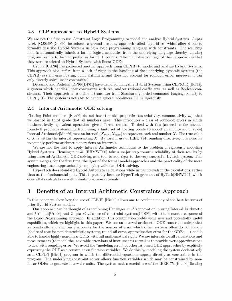
2.3 CLP approaches to Hybrid Systems

We are not the first to use Constraint Logic Programming to model and analyze Hybrid Systems. Guptaet al. [GJSB95][GJS96] introduced a ground breaking approach called “hybrid cc” which allowed one toformally describe Hybrid Systems using a logic programming language with constraints. The resultingmodels automatically inherit a formal logical semantics from the underlying language thereby allowingprogram results to be interpreted as formal theorems. The main disadvantage of their approach is thatthey were restricted to Hybrid Systems with linear ODEs.

Urbina [Urb96] has pioneered another approach using CLP(R) to model and analyze Hybrid Systems.This approach also suffers from a lack of rigor in the handling of the underlying dynamic systems (theCLP(R) system uses floating point arithmetic and does not account for roundoff error, moreover it canonly directly solve linear constraints).

Delzanno and Podelski [DP99][DP01] have explored analyzing Hybrid Systems using CLP(Q,R)[Hol95],a system which handles linear constraints with real and/or rational coefficients, as well as Boolean con-straints. Their approach is to define a translator from Shankar’s guarded command language[Sha93] toCLP(Q,R). The system is not able to handle general non-linear ODEs rigorously.

2.4 Interval Arithmetic ODE solving

Floating Point numbers [Kah96] do not have the nice properties (associativity, commutativity ...) thatwe learned in third grade that all numbers have. This introduces a class of round-off errors in whichmathematically equivalent operations give different results. To deal with this (as well as the obviousround-off problems stemming from using a finite set of floating points to model an infinite set of reals)Interval Arithmetic[Moo66] uses an interval (Xmin, Xmax) to represent each real number X. The true valueof X is within the interval representing X. By careful use of IEEE 754 rounding directives, it is possibleto soundly perform arithmetic operations on intervals.

We are not the first to apply Interval Arithmetic techniques to the problem of rigorously modelingHybrid Systems. Henzinger et al. [HHMWT00] take a major step towards reliability of their results byusing Interval Arithmetic ODE solving as a tool to add rigor to the very successful HyTech system. Thissystem merges, for the first time, the rigor of the formal model approaches and the practicality of the moreengineering-based approaches by employing validated ODE solving.

HyperTech does standard Hybrid Automata calculations while using intervals in the calculations, ratherthan as the fundamental unit. This is partially because HyperTech grew out of HyTech[HHWT97] whichdoes all its calculations with infinite precision rationals.

3 Benefits of an Interval Arithmetic Constraints Approach

In this paper we show how the use of CLP(F) [Hic00] allows one to combine many of the best features ofprior Hybrid System models.

Our approach can be thought of as combining Henzinger et al.’s innovation in using Interval Arithmeticand Urbina’s[Urb96] and Gupta et al.’s use of constraint systems[GJS96] with the semantic elegance ofthe Logic Programming approach. In addition, this combination yields some new and potentially usefulcapabilities, which we highlight in this paper. We use an interval arithmetic ODE constraint solver thatautomatically and rigorously accounts for the sources of error which other systems often do not handle(choice of case for non-deterministic systems, round-off error, approximation error for the ODEs, ...) and isable to handle highly non-linear ODEs with full mathematical rigor. We use intervals for all calculations andmeasurements (to model the inevitable error-bars of instruments) as well as to provide over-approximationsto deal with rounding error. We avoid the “modeling error” of other IA based ODE approaches by explicitlyexpressing the ODE as a constraint on function variables. We do this by modeling the system declarativelyas a CLP(F) [Hic01] program in which the differential equations appear directly as constraints in theprogram. The underlying constraint solver allows function variables which may be constrained by non-linear ODEs to generate interval results. The system makes careful use of the IEEE 754[Kah96] floating

2

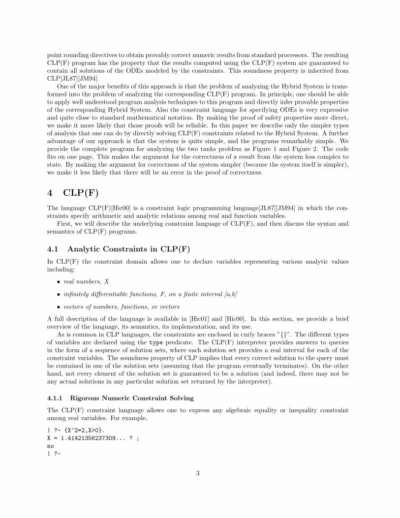
point rounding directives to obtain provably correct numeric results from standard processors. The resultingCLP(F) program has the property that the results computed using the CLP(F) system are guaranteed tocontain all solutions of the ODEs modeled by the constraints. This soundness property is inherited fromCLP[JL87][JM94].

One of the major benefits of this approach is that the problem of analyzing the Hybrid System is trans-formed into the problem of analyzing the corresponding CLP(F) program. In principle, one should be ableto apply well understood program analysis techniques to this program and directly infer provable propertiesof the corresponding Hybrid System. Also the constraint language for specifying ODEs is very expressiveand quite close to standard mathematical notation. By making the proof of safety properties more direct,we make it more likely that those proofs will be reliable. In this paper we describe only the simpler typesof analysis that one can do by directly solving CLP(F) constraints related to the Hybrid System. A furtheradvantage of our approach is that the system is quite simple, and the programs remarkably simple. Weprovide the complete program for analyzing the two tanks problem as Figure 1 and Figure 2. The codefits on one page. This makes the argument for the correctness of a result from the system less complex tostate. By making the argument for correctness of the system simpler (because the system itself is simpler),we make it less likely that there will be an error in the proof of correctness.

4 CLP(F)

The language CLP(F)[Hic00] is a constraint logic programming language[JL87][JM94] in which the con-straints specify arithmetic and analytic relations among real and function variables.

First, we will describe the underlying constraint language of CLP(F), and then discuss the syntax andsemantics of CLP(F) programs.

4.1 Analytic Constraints in CLP(F)

In CLP(F) the constraint domain allows one to declare variables representing various analytic valuesincluding:

• real numbers, X

• infinitely differentiable functions, F, on a finite interval [a,b]

• vectors of numbers, functions, or vectors

A full description of the language is available in [Hic01] and [Hic00]. In this section, we provide a briefoverview of the language, its semantics, its implementation, and its use.

As is common in CLP languages, the constraints are enclosed in curly braces ”{}”. The different typesof variables are declared using the type predicate. The CLP(F) interpreter provides answers to queriesin the form of a sequence of solution sets, where each solution set provides a real interval for each of theconstraint variables. The soundness property of CLP implies that every correct solution to the query mustbe contained in one of the solution sets (assuming that the program eventually terminates). On the otherhand, not every element of the solution set is guaranteed to be a solution (and indeed, there may not beany actual solutions in any particular solution set returned by the interpreter).

4.1.1 Rigorous Numeric Constraint Solving

The CLP(F) constraint language allows one to express any algebraic equality or inequality constraintamong real variables. For example,

| ?- {X^2=2,X>0}.X = 1.41421356237309... ? ;no| ?-

3

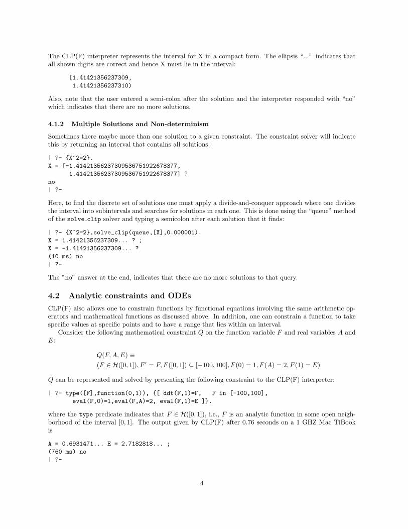
The CLP(F) interpreter represents the interval for X in a compact form. The ellipsis “...” indicates thatall shown digits are correct and hence X must lie in the interval:

[1.41421356237309,1.41421356237310)

Also, note that the user entered a semi-colon after the solution and the interpreter responded with “no”which indicates that there are no more solutions.

4.1.2 Multiple Solutions and Non-determinism

Sometimes there maybe more than one solution to a given constraint. The constraint solver will indicatethis by returning an interval that contains all solutions:

| ?- {X^2=2}.X = [-1.41421356237309536751922678377,

1.41421356237309536751922678377] ?no| ?-

Here, to find the discrete set of solutions one must apply a divide-and-conquer approach where one dividesthe interval into subintervals and searches for solutions in each one. This is done using the “queue” methodof the solve clip solver and typing a semicolon after each solution that it finds:

| ?- {X^2=2},solve_clip(queue,[X],0.000001).X = 1.41421356237309... ? ;X = -1.41421356237309... ?(10 ms) no| ?-

The ”no” answer at the end, indicates that there are no more solutions to that query.

4.2 Analytic constraints and ODEs

CLP(F) also allows one to constrain functions by functional equations involving the same arithmetic op-erators and mathematical functions as discussed above. In addition, one can constrain a function to takespecific values at specific points and to have a range that lies within an interval.

Consider the following mathematical constraint Q on the function variable F and real variables A andE:

Q(F,A,E) ≡(F ∈ H([0, 1]), F ′ = F, F ([0, 1]) ⊆ [−100, 100], F (0) = 1, F (A) = 2, F (1) = E)

Q can be represented and solved by presenting the following constraint to the CLP(F) interpreter:

| ?- type([F],function(0,1)), {[ ddt(F,1)=F, F in [-100,100],eval(F,0)=1,eval(F,A)=2, eval(F,1)=E ]}.

where the type predicate indicates that F ∈ H([0, 1]), i.e., F is an analytic function in some open neigh-borhood of the interval [0, 1]. The output given by CLP(F) after 0.76 seconds on a 1 GHZ Mac TiBookis

A = 0.6931471... E = 2.7182818... ;(760 ms) no| ?-

4

which represents the following answer constraint:

C(F,A,E) ≡ (A ∈ [0.6931471, 0.6931472) ∧ E ∈ [2.7182818, 2.7182819))

The soundness of the CLP(F) interpreter implies that it has proven a theorem about the query and itssolution constraint:

∀F,A,E Q(F,A,E)⇒ C(F,A,E)

In other words, if F , A, and E represent a solution to Q, then they must satisfy the answer constraint C.Note that one cannot infer from this theorem that Q has any solutions at all. In this particular case, Qclearly does have a solution

F (t) = exp(t), A = ln(2), E = e

which of course satisfies the answer constraint C.The CLP(F) system solves analytic constraints by soundly approximating analytic functions by power

series and introducing arithmetic constraints among the Taylor coefficients of the functions at the endpoints,at points in the interval, and over the entire range. For more details consult [Hic00].

4.3 Programs

CLP(F) programs are Prolog programs in which the bodies of rules may contain CLP(F) constraints.CLP(F) provides the full power of Prolog in addition to the power of the underlying constraint solver andboth are combined within a single logical semantics. Moreover, by the soundness and completeness of CLP[JM94] semantics, if a CLP interpreter returns N solutions sets C1, . . . , Cn for a query Q(X,F ) and thenhalts, then every solution of the query Q(X,F ) consisting of a real vector X and a vector F of real-valuedfunctions, is contained in the union of the solution sets Ci.

The logical semantics of CLP(F) programs can be summarized in the following theorem [Hic00]

Theorem 1 Let P be a CLP(F) program, Q(x) a CLP(F) query where x is a tuple of real variables, andassume the interpreter returns N answer constraints {x ∈ Ij} for tuples of intervals I1, . . . , IN . Let P ∗ bethe first order theory obtained from a logic reading of P (by Clark’s Completion Semantics [Cla78][LLo87]),and let T be the first order theory of the domain F of analytic functions on real intervals. Then one caninfer that

P ∗ ∪ T ` ∀x

Q(x)⇒ x ∈⋃j

Ij

Theorem 2 Notation as in the previous theorem. If the interpreter halts with no answer constraints (i.e.,N=0), then one can infer

P ∗ ∪ T ` ¬∃x Q(x)

i.e., the query is not satisfiable.

This theorem allows one to infer correctness of a CLP(F) simulator for a Hybrid System as well assafety properties of the System directly from the corresponding CLP(F) program. We now illustrate thisusing the Two Tanks example.

5 Two Tanks in CLP

5.1 Description of the Two Tanks Problems

The “Two Tanks” problem is to accurately model a system consisting of two water tanks. There is a flowof water in to the higher tank, and a horizontal pipe from the bottom of the higher tank to some point inthe side of the lower tank. There is an outflow pipe at the bottom of the lower tank. In some versions of

5

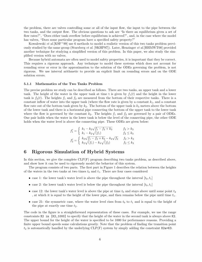
the problem, there are valves controlling some or all of the input flow, the input to the pipe between thetwo tanks, and the output flow. The obvious questions to ask are “Is there an equilibrium given a set offlow rates?”, “Does either tank overflow before equilibrium is achieved?”, and, in the case where the modelhas valves, “Does some particular program have a specified safety property?”

Kowalewski et al.[KSF+99] use 6 methods to model a realistic version of this two tanks problem previ-ously studied by the same group (Stursberg et al. [SKHP97]). Later, Henzinger et al.[HHMWT00] providedanother technique for studying a simplified version of this problem. In this paper, we also study the sim-plified version with no valves.

Because hybrid automata are often used to model safety properties, it is important that they be correct.This requires a rigorous approach. Any technique to model these systems which does not account forrounding error or error in the approximation to the solution of the ODEs governing the problem, is notrigorous. We use interval arithmetic to provide an explicit limit on rounding errors and on the ODEsolution errors.

5.1.1 Mathematics of the Two Tanks Problem

The precise problem we study can be described as follows. There are two tanks, an upper tank and a lowertank. The height of the water in the upper tank at time t is given by f1(t) and the height in the lowertank is f2(t). The heights f1 and f2 are measured from the bottom of their respective tanks. There is aconstant inflow of water into the upper tank (where the flow rate is given by a constant k1, and a constantflow rate out of the bottom tank given by k2. The bottom of the upper tank is k3 meters above the bottomof the lower tank and there is a horizontal pipe connecting the bottom of the upper tank to the lower tankwhere the flow is governed by the constant k2. The heights f1 and f2 are governed by a pair of ODEs.One pair holds when the water in the lower tank is below the level of the connecting pipe, the other ODEholds when the water level is above the connecting pipe. These ODEs are given below:

f ′1 ={k1 − k2

√f1 − f2 + k3 f2 > k3

k1 − k2

√(f1) f2 ≤ k3

f ′2 ={k2

√f1 − f2 + k3 − k4

√f2 f2 > k3

k2

√(f1)− k4

√(f2) f2 ≤ k3

6 Rigorous Simulation of Hybrid Systems

In this section, we give the complete CLP(F) program describing two tanks problem, as described above,and show how it can be used to rigorously model the behavior of this system.

The program consists of two parts. The first part in Figure 1 describes the relation between the heightsof the waters in the two tanks at two times t0 and t1. There are four cases considered

• case 1: the lower tank’s water level is above the pipe throughout the interval [t0, t1]

• case 2: the lower tank’s water level is below the pipe throughout the interval [t0, t1]

• case 12: the lower tank’s water level is above the pipe at time t0 and stays above until some point t2, at which it is equal to the height of the lower pipe, and then remains below the pipe until time t1.

• case 21: the symmetric case, where the water level rises from t0 to t1 and is equal to the height ofthe pipe at exactly one time t2.

The code in the figure is a straightforward representation of these cases. For example, we use the rangeconstraints X2 in [K2,1000] to specify that the height of the water in the second tank is always above K2.The upper bound for the height of the water is specified to be 1000 for performance reasons. Providing afinite upper bound speeds some calculations greatly. Note that the problem of finding the transition pointt2 is automatically handled by the underlying CLP(F) system by simply adding the constraint X2a=K3.

6

twotank(case1,X10,X20,T0,X11,X21,T1,[K1,K2,K3,K4]) :-decls([X1,X2],function(T0,T1)),

{[ ddt(X1,1) = K1 - K2*psqrt(X1-X2+K3),ddt(X2,1) = K2*psqrt(X1-X2+K3) - K4*psqrt(X2),eval(X1,T0)=X10, eval(X1,T1)=X11,eval(X2,T0)=X20, eval(X2,T1)=X21,X1 in [E,1000], X2 in [K3,1000],

]}.

twotank(case2,X10,X20,T0,X11,X21,T1,[K1,K2,K3,K4]) :-decls([X1,X2,Z1,Z2],function(T0,T1)),

{[ ddt(X1,1) = K1 - K2*psqrt(X1),ddt(X2,1) = K2*psqrt(X1) - K4*psqrt(X2),eval(X1,T0)=X10, eval(X1,T1)=X11,eval(X2,T0)=X20, eval(X2,T1)=X21,X1 in [E,1000], X2 in [E,K3],

]}..twotank(case12,X10,X20,T0,X11,X21,T1,Ks) :-

{T0=<Ta, Ta<T1},Ks=[_,_,K3,_],{X2a=K3},twotank(case1,X10,X20,T0,X1a,X2a,Ta,Ks),nl,nl,print(case12(X1a,X2a,Ta)),nl,nl,twotank(case2,X1a,X2a,Ta,X11,X21,T1,Ks).

twotank(case21,X10,X20,T0,X11,X21,T1,Ks) :-{T0=<Ta, Ta<T1}, Ks=[_,_,K3,_],{X2a=K3},twotank(case2,X10,X20,T0,X1a,X2a,Ta,Ks),nl,nl,print(case21(X1a,X2a,Ta)),nl,nl,twotank(case1,X1a,X2a,Ta,X11,X21,T1,Ks).

% equilibrium is at X10=0.625, X20=0.5625,ks([K1,K2,K3,K4]) :- K2=1, K4=1, % sqrt(meters)/second

K3=0.5, % metersK1= 0.75 % meters/sec

Figure 1: CLP(F) code for Case1, Case2, and transitions between them

7

iterate(N,_DT,X10,X20,T0,X10,X20,T0,_Ks) :- {N<0},fail.iterate(N,_DT,X10,X20,T0,X10,X20,T0,_Ks) :- {N=0}.iterate(N,DT,X10,X20,T0,X11,X21,T1,Ks) :- {T1a=T0+DT, N1=N-1},forward_chk([X1a,X2a,T1a], twotank(Case,X10,X20,T0,X1a,X2a,T1a,Ks))iterate(N1,DT,X1a,X2a,T1a,X11,X21,T1,Ks).

Figure 2: CLP(F) code for iterating to find a fixpoint

The second part of the program is an iterator (Figure 2) that repeatedly steps through the time domainapplying the appropriate case (or when nondeterminism is present, cases) to compute the current waterlevels in the two tanks. This program makes the assumption that the water level does not cross the heightof the pipe more than once in any DT interval. We could handle this by making the program a little morecomplex, but for presentation purposes we stick to this simple case for now. (We would need to use anadaptive step size when switching from case 1 to case 2 or back). Also, the forward_chk call is used as aspace optimization to minimize the size of the constraint set.

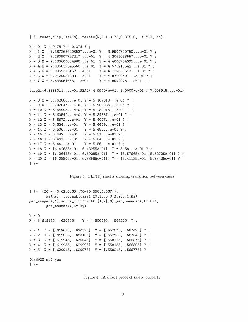
This program can now be executed by loading it into the CLP(F) interpreter and posing queries. Forexample, in Figure 3 we show the (slightly edited) output results of a query that rigorously follows thewater levels over a period of two seconds with 0.1 second steps. Note that it finds the transition point fromcase 2 to case 1 automatically.

7 Rigorous Analysis of Hybrid Systems

The same program can be used to prove properties of the two tanks system. In this section we show howto prove the following safety property, which states that if the tank levels are ever sufficiently close to an“equilibrium” point, then they stay relatively near that point forever, more precisely

If the tank levels X0 for the upper tank and Y0 for the lower tank satisfy

0.62 ≤ X0 ≤ 0.63 ∧ 0.558 ≤ Y0 ≤ 0.567

at time 0, then for all times t in the future the tank levels X and Y satisfy

0.61922 ≤ X ≤ 0.63083 ∧ 0.55674 ≤ Y ≤ 0.56815

We prove this in two steps. First we prove that if the tank levels are in the initial interval [0.62, 0.63]×[0.558, 0.567] at time 0, then they are also in that interval at time 0.1. This implies that they are in thatinterval at time N ∗ 0.1 for all N . Next we prove that if they start in the given interval at time 0, thenthey are in the second stated interval at all times t with 0 ≤ t ≤ 0.1. This proves the safety property.

The first part can be proved directly by using the “solve clip” solver which provides increasingly moreprecise bounds on the answer constraint as shown in Figure 4. This corresponds to the standard IntervalArithmetic ODE solving approach. In our system, it takes about 10 minutes to prove this directly.

Another approach is to use constraints and try to find an initial point (X,Y ) such that after 0.1 secondsit is “out of the box”. This is specified by the query in Figure 5. As can be seen, this returns with a “no”answer, which means no such point exists and hence all such (X,Y ) must end up inside the “box”. Thecalculation takes about 3 seconds and is more elegant than the direct approach

The last part of the proof, involves computing the range of possible values of (X,Y ) over the interval[0, 0.1] assuming they start in the specified box. This is done by making the query in Figure 6. in about2.3 seconds.

8 Advantages

There are several advantages to our approach.

8

| ?- reset_clip, ks(Ks),iterate(N,0.1,0.75,0.375,0, X,Y,T, Ks).

N = 0 X = 0.75 Y = 0.375 ? ;N = 1 X = 7.3872686208537...e-01 Y = 3.9904710750...e-01 ? ;N = 2 X = 7.280907797217...e-01 Y = 4.2065058557...e-01 ? ;N = 3 X = 7.180600004968...e-01 Y = 4.4006784395...e-01 ? ;N = 4 X = 7.086039345668...e-01 Y = 4.575212542...e-01 ? ;N = 5 X = 6.9969315162...e-01 Y = 4.732050513...e-01 ? ;N = 6 X = 6.9129937388...e-01 Y = 4.87290407...e-01 ? ;N = 7 X = 6.833954653...e-01 Y = 4.9992926...e-01 ? ;

case21(6.8335011...e-01,REAL([4.9999*e-01, 5.0000*e-01]),7.005915...e-01)

N = 8 X = 6.762886...e-01 Y = 5.109318...e-01 ? ;N = 9 X = 6.702047...e-01 Y = 5.202036...e-01 ? ;N = 10 X = 6.64998...e-01 Y = 5.280075...e-01 ? ;N = 11 X = 6.60542...e-01 Y = 5.34567...e-01 ? ;N = 12 X = 6.5672...e-01 Y = 5.4007...e-01 ? ;N = 13 X = 6.534...e-01 Y = 5.4469...e-01 ? ;N = 14 X = 6.506...e-01 Y = 5.485...e-01 ? ;N = 15 X = 6.482...e-01 Y = 5.51...e-01 ? ;N = 16 X = 6.461...e-01 Y = 5.54...e-01 ? ;N = 17 X = 6.44...e-01 Y = 5.56...e-01 ? ;N = 18 X = [6.42685e-01, 6.43255e-01] Y = 5.58...e-01 ? ;N = 19 X = [6.26485e-01, 6.69285e-01] Y = [5.57665e-01, 5.62725e-01] ? ;N = 20 X = [6.08805e-01, 6.88585e-01]) Y = [5.41135e-01, 5.78425e-01] ?| ?-

Figure 3: CLP(F) results showing transition between cases

| ?- {X0 = [0.62,0.63],Y0=[0.558,0.567]},ks(Ks), twotank(case1,X0,Y0,0.0,X,Y,0.1,Ks)

get_range(X,Y),solve_clip(fwchk,[X,Y],N),get_bounds(X,Lx,Hx),get_bounds(Y,Ly,Hy).

N = 0X = [.619185, .630855] Y = [.556695, .568205] ? ;

N = 1 X = [.619615, .630375] Y = [.557575, .567425] ? ;N = 2 X = [.619835, .630155] Y = [.557955, .567045] ? ;N = 3 X = [.619945, .630045] Y = [.558115, .566875] ? ;N = 4 X = [.619985, .629995] Y = [.558185, .566805] ? ;N = 5 X = [.620015, .629975] Y = [.558215, .566775] ?

(633920 ms) yes| ?-

Figure 4: IA direct proof of safety property

9

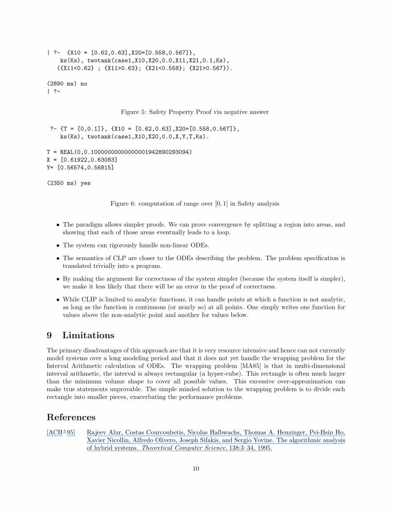
| ?- {X10 = [0.62,0.63],X20=[0.558,0.567]},ks(Ks), twotank(case1,X10,X20,0.0,X11,X21,0.1,Ks),({X11<0.62} ; {X11>0.63}; {X21<0.558}; {X21>0.567}).

(2890 ms) no| ?-

Figure 5: Safety Property Proof via negative answer

?- {T = [0,0.1]}, {X10 = [0.62,0.63],X20=[0.558,0.567]},ks(Ks), twotank(case1,X10,X20,0.0,X,Y,T,Ks).

T = REAL(0,0.10000000000000001942890293094)X = [0.61922,0.63083]Y= [0.56574,0.56815]

(2350 ms) yes

Figure 6: computation of range over [0, 1] in Safety analysis

• The paradigm allows simpler proofs. We can prove convergence by splitting a region into areas, andshowing that each of those areas eventually leads to a loop.

• The system can rigorously handle non-linear ODEs.

• The semantics of CLP are closer to the ODEs describing the problem. The problem specification istranslated trivially into a program.

• By making the argument for correctness of the system simpler (because the system itself is simpler),we make it less likely that there will be an error in the proof of correctness.

• While CLIP is limited to analytic functions, it can handle points at which a function is not analytic,as long as the function is continuous (or nearly so) at all points. One simply writes one function forvalues above the non-analytic point and another for values below.

9 Limitations

The primary disadvantages of this approach are that it is very resource intensive and hence can not currentlymodel systems over a long modeling period and that it does not yet handle the wrapping problem for theInterval Arithmetic calculation of ODEs. The wrapping problem [MA85] is that in multi-dimensionalinterval arithmetic, the interval is always rectangular (a hyper-cube). This rectangle is often much largerthan the minimum volume shape to cover all possible values. This excessive over-approximation canmake true statements unprovable. The simple minded solution to the wrapping problem is to divide eachrectangle into smaller pieces, exacerbating the performance problems.

References

[ACH+95] Rajeev Alur, Costas Courcoubetis, Nicolas Halbwachs, Thomas A. Henzinger, Pei-Hsin Ho,Xavier Nicollin, Alfredo Olivero, Joseph Sifakis, and Sergio Yovine. The algorithmic analysisof hybrid systems. Theoretical Computer Science, 138:3–34, 1995.

10

[BO97] Frederic Benhamou and William J. Older. Applying interval arithmetic to real, integer, andboolean constraints. Journal of Logic Programming, 32(1):1–24, Jul 1997.

[Cla78] Keith Clark. Negation as failure. In Herve Gallaire and Jack Minker, editors, Logic andDatabases, pages 293–322. Plenum Press, New York, NY, 1978.

[DN00] J.M. Davoren and Anil Nerode. Logics for hybrid systems. Proceedings of the IEEE,88(7):985–1010, Jul 2000.

[DP99] Giorgio Delzanno and Andreas Podelski. Model checking in CLP. In Rance Cleaveland,editor, Proceedings of the Fifth International Conference on Tools and Algorithms for theConstruction and Analysis of Systems (TACAS ’99), volume 1579 of LNCS, pages 223–239.Springer Verlag, 1999.

[DP01] Giorgio Delzanno and Andreas Podelski. Constraint-based deductive model checking. Inter-national Journal on Software Tools for Technology Transfer (STTT), 3(3), 2001.

[GJS96] Vineet Gupta, Radha Jagadeesan, and Vijay Saraswat. Hybrid cc, hybrid automata andprogram verification. In Rajeev Alur, Thomas A. Henzinger, and Eduardo D. Sontag, editors,Hybrid Systems III: Verification and Control, volume 1066 of LNCS, pages 52–63. SpringerVerlag, 1996.

[GJSB95] Vineet Gupta, Radha Jagadeesan, Vijay Saraswat, and Daniel G. Bobrow. Programmingin hybrid constraint languages. In Panos Antsaklis, Wolf Kohn, Anil Nerode, and ShankarSastry, editors, Hybrid Systems II, volume 999 of LNCS, pages 226–251. Springer Verlag,1995.

[Hen96] Thomas A. Henzinger. The theory of hybrid automata. In Proceedings, 11th Symposium onLogic in Computer Science (LICS ’96), pages 278–292. IEEE Computer Society Press, 1996.

[HHMWT00] Thomas A. Henzinger, Benjamin Horowitz, Rupak Majumdar, and Howard Wong-Toi. Be-yond HyTech: Hybrid systems analyis using interval numerical methods. In Nancy Lynchand Bruce H. Krogh, editors, Hybrid Systems: Computation and Control (HSCC 2000),volume 1790 of LNCS, pages 130–144. Springer Verlag, 2000.

[HHWT97] Thomas A. Henzinger, Pei-Hsin Ho, and Howard Wong-Toi. HyTech: A model checker forhybrid systems. Software Tools for Technology Transfer, 1(?):110–122, 1997.

[HHWT98] Thomas A. Henzinger, Pei-Hsin Ho, and Howard Wong-Toi. Algorithmic analysis of nonlinearhybrid systems. IEEE Transactions on Automatic Control, 43:540–554, 1998.

[Hic00] Timothy J. Hickey. Analytic constraint solving and interval arithmetic. In POPL’00 ACMSIGPLAN-SIGACT Symposium on Principles of Programming Languages, pages 338–351,2000. published as vol. 27 of SIGPLAN notices.

[Hic01] Timothy J. Hickey. Metalevel interval arithmetic and verifiable constraint solving. Jour-nal of Functional and Logic Programming, 2001(7), October 2001. http://danae.uni-muenster.de/lehre/kuchen/JFLP/articles/2001/S01-02/JFLP-A01-07.pdf.

[Hol95] C. Holzbaur. OFAI clp(q,r) Manual. Austrian Research Institute for Artificial Intelligence,Vienna, 1.3.3 edition, 1995. TR-95-05.

[JL87] J. Jaffar and J.L. Lassez. Constraint logic programming. In Proceedings 14th ACM Sympo-sium on the Principles of Programming Languages, pages 111–119, 1987.

[JM94] Joxan Jaffar and Michael J. Maher. Constraint logic programming: A survey. Journal ofLogic Programming, 19/20:503–581, 1994.

11

[Kah96] W. Kahan. Lecture notes on the status of ieee standard 754 for binary floating-point arith-metic. Technical report, EECS, University of California, Berkely, 1996.

[KSF+99] S. Kowalewski, O. Stursberg, M. Fritz, H. Graf, I. Hoffman, J. Preußig, M. Remelhe, S. Si-mon, and H. Treseler. A case study in tool-aided analysis of discretely controlled continuoussystems: The two tanks problem. In Panos Antsaklis, Wolf Kohn, Michael Lemmon, AnilNerode, and Shankar Sastry, editors, Hybrid Systems V, volume 1567 of LNCS, pages 163–185. Springer Verlag, 1999.

[LLo87] John Wylie LLoyd. Foundations of Logic Programming. Springer, second, expanded edition,1987.

[LSV01] Nancy Lynch, Roberto Segala, and Frits Vaandrager. Hybrid I/O automata revisited. InMaria Domenica Di Benedetto and Alberto Sangiovanni-Vincentelli, editors, HSCC, number2034 in LNCS, pages 403–417. Springer Verlag, 2001.

[LSVW99] Nancy Lynch, Roberto Segala, Frits W. Vaandrager, and H.B. Weinberg. Hybrid I/O au-tomata. Technical Report CSI-R9907, Computing Science Institue Nijmegen; Faculty ofMathematics and Informatics; Catholic University of Nijmegen, Toernooivveld 1; 6525 EDNijmegen; The Netherlands, Apr 1999.

[MA85] S. Markov and R. Angelov. An interval method for systems of ODE. In Karl Nickel, editor,Interval Mathematics 1985, volume 212 of LNCS, pages 103–108. Springer, 1985.

[MMP91] Oded Maler, Zohar Manna, and Amir Pnueli. From timed to hybrid systems. In J.W.de Bakker, C. Huizing, W.P. de Roever, and G. Rozenberg, editors, Real-Time: Theory inPractice, volume 600 of LNCS, pages 447–484. Rex Workshop, Springer Verlag, 1991.

[Moo66] Ramon E. Moore. Interval Analysis. Prentice-Hall, 1966.

[Sha93] A. Udaya Shankar. An introduction to assertional reasoning for concurrent systems. ACMComputing Surveys, 25(3):225–262, Sep 1993.

[SKHP97] Olaf Stursberg, Stefan Kowalewski, Ingo Hoffman, and Jorg Preußig. Comparing timed andhybrid automata as approximations of continuous systems. In Panos Antsaklis, Wolf Kohn,Anil Nerode, and Shankar Sastry, editors, Hybrid Systems IV, volume 1273 of LNCS, pages361–377. Springer Verlag, 1997.

[Urb96] Luis Urbina. Analysis of hybrid systems in CLP(R). In Eugene C. Freuder, editor, Principlesand Practice of Constraint Programming – CP96, volume 1118 of LNCS, pages 451–467.Springer, Aug 1996.

12