Rigorous System-level Modeling and Performance Evaluation ...
208
HAL Id: tel-01148690 https://tel.archives-ouvertes.fr/tel-01148690 Submitted on 5 May 2015 HAL is a multi-disciplinary open access archive for the deposit and dissemination of sci- entific research documents, whether they are pub- lished or not. The documents may come from teaching and research institutions in France or abroad, or from public or private research centers. L’archive ouverte pluridisciplinaire HAL, est destinée au dépôt et à la diffusion de documents scientifiques de niveau recherche, publiés ou non, émanant des établissements d’enseignement et de recherche français ou étrangers, des laboratoires publics ou privés. Rigorous System-level Modeling and Performance Evaluation for Embedded System Design Ayoub Nouri To cite this version: Ayoub Nouri. Rigorous System-level Modeling and Performance Evaluation for Embedded System Design. Other [cs.OH]. Université Grenoble Alpes, 2015. English. NNT : 2015GREAM008. tel- 01148690
-
Upload
khangminh22 -
Category
Documents
-
view
1 -
download
0
Transcript of Rigorous System-level Modeling and Performance Evaluation ...

HAL Id: tel-01148690https://tel.archives-ouvertes.fr/tel-01148690
Submitted on 5 May 2015
HAL is a multi-disciplinary open accessarchive for the deposit and dissemination of sci-entific research documents, whether they are pub-lished or not. The documents may come fromteaching and research institutions in France orabroad, or from public or private research centers.
L’archive ouverte pluridisciplinaire HAL, estdestinée au dépôt et à la diffusion de documentsscientifiques de niveau recherche, publiés ou non,émanant des établissements d’enseignement et derecherche français ou étrangers, des laboratoirespublics ou privés.
Rigorous System-level Modeling and PerformanceEvaluation for Embedded System Design
Ayoub Nouri
To cite this version:Ayoub Nouri. Rigorous System-level Modeling and Performance Evaluation for Embedded SystemDesign. Other [cs.OH]. Université Grenoble Alpes, 2015. English. �NNT : 2015GREAM008�. �tel-01148690�
THÈSEPour obtenir le grade de
DOCTEUR DE L’UNIVERSITÉ DE GRENOBLESpécialité : Informatique
Arrêté ministérial : 7 août 2006
Présentée par
Ayoub Nouri
Thèse dirigée par Saddek Bensalemet codirigée par Marius Bozga
préparée au sein du laboratoire Verimaget de l’École Doctorale Mathématique, Science et Technologie de l’In-formation, Informatique (MSTII)
Rigorous System-level Modelingand Performance Evaluation forEmbedded Systems Design
Thèse soutenue publiquement le 8 avril 2015,devant le jury composé de :
M. Jean Claude FernandezProfesseur, Université de Grenoble, PrésidentM. Albert CohenDirecteur de recherche, INRIA, RapporteurM. Radu GrosuProfesseur, Vienna University of Technology, RapporteurM. Kamel BarkaouiProfesseur, Conservatoire National des Arts et Métiers, ExaminateurM. Ahmed BouajjaniProfesseur, Université Paris Diderot, ExaminateurM. Saddek BensalemProfesseur, Université de Grenoble, Directeur de thèseM. Marius BozgaIngénieur de recherche – HDR, CNRS, Co-Directeur de thèseM. Axel LegayChargé de recherche, INRIA, Co-Encadrant de thèse


Acknowledgments
Foremost, I would like to thank Saddek Bensalem for giving me the opportu-nity to join Verimag and to achieve my PhD work under his supervision. Heoffered me motivation, valuable research directions, and more importantly,a very nice working environment that helped me to accomplish this work.
I am deeply thankful to Marius Bozga, my co-advisor, for his availability,his valuable advice, and for the long and rich discussions, often beyond thework scope. Without his help, this work could never have been the same.
A great thank goes to Axel Legay for assisting and inspiring me in variousparts of the work. Especially, the stochastic extension of the BIP frameworkand the statistical model checking technique.
I am very grateful to all the jury members for accepting to review thiswork and for their valuable feedback on the manuscript and the presentation.
I want also to thank people from CEA Grenoble, the LIALP group, fortheir collaboration on the HMAX case study, and professor Bernard Ycartfrom University of Grenoble for his help on statistical aspects.
I want to thank all my colleges at Verimag for the nice, healthy, and richworking environment, all the administrative staff for their help and assis-tance. A wink to the Verimag football team. I also thank Yassine Lacknechfor giving me the opportunity to make an internship at Verimag in 2010.
Finally, I would like to thank my family : my parents, my brothers, mysister, and my in-laws, for their support and their affection. A special thankto my beloved wife for her unconditional support. Without her by my sidethis work could never have been achieved.


I dedicate this work to my family

Abstract
In the present work, we tackle the problem of modeling and evaluatingperformance in the context of embedded systems design. These have becomeessential for modern societies and experienced important evolution. Due tothe growing demand on functionality and programmability, software solu-tions have gained in importance, although known to be less efficient thandedicated hardware. Consequently, considering performance has become amust, especially with the generalization of resource-constrained devices.
We present a rigorous and integrated approach for system-level perfor-mance modeling and analysis. The proposed method enables faithful high-level modeling, encompassing both functional and performance aspects, andallows for rapid and accurate quantitative performance evaluation. Theapproach is model-based and relies on the SBIP formalism for stochasticcomponent-based modeling and formal verification. We use statistical modelchecking for analyzing performance requirements and introduce a stochasticabstraction technique to enhance its scalability. Faithful high-level modelsare built by calibrating functional models with low-level performance infor-mation using automatic code generation and statistical inference.
We provide a tool-flow that automates most of the steps of the proposedapproach and illustrate its use on a real-life case study for image process-ing. We consider the design and mapping of a parallel version of the HMAXmodels algorithm for object recognition on the STHORM many-cores plat-form. We explored timing aspects and the obtained results show not onlythe usability of the approach but also its pertinence for taking well-foundeddecisions in the context of system-level design.


Résumé
Les systèmes embarqués ont évolué d’une manière spectaculaire et sontdevenus partie intégrante de notre quotidien. En réponse aux exigences gran-dissantes en termes de nombre de fonctionnalités et donc de flexibilité, lesparties logicielles de ces systèmes se sont vues attribuer une place importantemalgré leur manque d’efficacité, en comparaison aux solutions matérielles.Par ailleurs, vu la prolifération des systèmes nomades et à ressources limi-tés, tenir compte de la performance est devenu indispensable pour bien lesconcevoir.
Dans cette thèse, nous proposons une démarche rigoureuse et intégréepour la modélisation et l’évaluation de performance tôt dans le processus deconception. Cette méthode permet de construire des modèles, au niveau sys-tème, conformes aux spécifications fonctionnelles, et intégrant les contraintesnon-fonctionnelles de l’environnement d’exécution. D’autre part, elle permetd’analyser quantitativement la performance de façon rapide et précise. Cetteméthode est guidée par les modèles et se base sur le formalisme SBIP quenous proposons pour la modélisation stochastique selon une approche for-melle et par composants.
Pour construire des modèles conformes, nous partons de modèles pure-ment fonctionnels utilisés pour générer automatiquement une implémenta-tion distribuée, étant donnée une architecture matérielle cible et un schémade répartition. Dans le but d’obtenir une description fidèle de la performance,nous avons conçu une technique d’inférence statistique qui produit une ca-ractérisation probabiliste. Cette dernière est utilisée pour calibrer le modèlefonctionnel de départ. Afin d’évaluer la performance de ce modèle, nous nousbasons sur du model checking statistique que nous améliorons à l’aide d’unetechnique d’abstraction.
Nous avons développé un flot de conception qui automatise la majoritédes phases décrites ci-dessus. Ce flot a été appliqué à différentes études decas, notamment à une application de reconnaissance d’image déployée sur laplateforme multi-cœurs STHORM.


Contents
1 Introduction 1
1.1 Motivation and Methodology . . . . . . . . . . . . . . . . . . 1
1.2 Embedded Systems Design . . . . . . . . . . . . . . . . . . . . 3
1.2.1 Design and Challenges . . . . . . . . . . . . . . . . . . 3
1.2.2 System-level Design . . . . . . . . . . . . . . . . . . . 5
1.2.3 State of the Art . . . . . . . . . . . . . . . . . . . . . . 8
1.3 Performance in System-level Design . . . . . . . . . . . . . . . 10
1.3.1 Challenges . . . . . . . . . . . . . . . . . . . . . . . . . 11
1.3.2 Performance Modeling Requirements . . . . . . . . . . 12
1.3.3 Performance Evaluation Requirements . . . . . . . . . 17
1.4 Contributions and Organization . . . . . . . . . . . . . . . . . 19
1.4.1 System-level Modeling . . . . . . . . . . . . . . . . . . 20
1.4.2 System-level Verification . . . . . . . . . . . . . . . . . 21
1.4.3 Integrated Performance Modeling and Analysis . . . . 22
I Formalisms and Techniques 23
2 Quantitative Analysis of Stochastic Models: A Background 25
2.1 Stochastic Systems Modeling . . . . . . . . . . . . . . . . . . 26
2.1.1 Discrete Time Markov Chains . . . . . . . . . . . . . . 26
2.1.2 Markov Decision Process . . . . . . . . . . . . . . . . . 29
2.2 Requirements Formalization . . . . . . . . . . . . . . . . . . . 32
2.2.1 Linear-time Temporal Logic . . . . . . . . . . . . . . . 32
2.3 Statistical Model Checking . . . . . . . . . . . . . . . . . . . . 33
2.3.1 Probabilistic Bounded LTL . . . . . . . . . . . . . . . 35
2.3.2 Qualitative Analysis . . . . . . . . . . . . . . . . . . . 35
2.3.3 Quantitative Analysis . . . . . . . . . . . . . . . . . . 36
2.3.4 Playing with Statistical Model Checking Algorithms . 37
2.4 Conclusions and Related Work . . . . . . . . . . . . . . . . . 37
xi

xii CONTENTS
3 Stochastic Component-based Modeling 41
3.1 Background on BIP . . . . . . . . . . . . . . . . . . . . . . . . 42
3.1.1 Atomic Components . . . . . . . . . . . . . . . . . . . 42
3.1.2 Composition Operators . . . . . . . . . . . . . . . . . 45
3.2 SBIP: A Stochastic Extension . . . . . . . . . . . . . . . . . . 50
3.2.1 Stochastic Atomic Components . . . . . . . . . . . . . 50
3.2.2 Composition of Stochastic Components . . . . . . . . 55
3.2.3 Purely Stochastic Semantics . . . . . . . . . . . . . . . 57
3.3 Performance Evaluation of a Multimedia SoC . . . . . . . . . 60
3.3.1 SBIP Model of the Multimedia SoC . . . . . . . . . . 61
3.3.2 QoS Requirements Evaluation . . . . . . . . . . . . . . 64
3.4 SBIP Expressiveness . . . . . . . . . . . . . . . . . . . . . . . 68
3.4.1 Modeling LMCs in SBIP . . . . . . . . . . . . . . . . 68
3.4.2 Modeling MDPs in SBIP . . . . . . . . . . . . . . . . 72
3.5 Conclusions . . . . . . . . . . . . . . . . . . . . . . . . . . . . 77
4 Stochastic Abstraction 79
4.1 Preliminaries . . . . . . . . . . . . . . . . . . . . . . . . . . . 81
4.1.1 Additional Stochastic Models . . . . . . . . . . . . . . 81
4.1.2 Probabilistic Learning Techniques . . . . . . . . . . . . 81
4.2 Abstraction via Learning and Projection . . . . . . . . . . . . 83
4.2.1 Abstraction Steps . . . . . . . . . . . . . . . . . . . . . 84
4.2.2 Correctness Statement . . . . . . . . . . . . . . . . . . 86
4.3 Herman’s Self Stabilizing Algorithm . . . . . . . . . . . . . . 88
4.4 Conclusions and Related Work . . . . . . . . . . . . . . . . . 93
II Methods and Flow 97
5 Rigorous System-level Performance Modeling and Analysis 99
5.1 ASTROLABE : An Integrated Approach . . . . . . . . . . . . 100
5.1.1 Answering General Design Challenges . . . . . . . . . 100
5.1.2 Answering Performance Specific Challenges . . . . . . 101
5.2 Gathering Low-level Performance Details . . . . . . . . . . . . 104
5.2.1 Automatic Implementation Generation . . . . . . . . . 104
5.2.2 Instrumentation . . . . . . . . . . . . . . . . . . . . . 105
5.3 Characterizing Performance Information . . . . . . . . . . . . 105
5.4 Calibrating Functional Models . . . . . . . . . . . . . . . . . . 108
5.4.1 Timing Information . . . . . . . . . . . . . . . . . . . 108
5.5 Conclusions . . . . . . . . . . . . . . . . . . . . . . . . . . . . 113
CONTENTS xiii
6 Statistical Characterization of Performance 1156.1 Statistical Inference . . . . . . . . . . . . . . . . . . . . . . . . 1156.2 Distribution Fitting . . . . . . . . . . . . . . . . . . . . . . . 117
6.2.1 Exploratory Analysis . . . . . . . . . . . . . . . . . . . 1176.2.2 Parameters Estimation . . . . . . . . . . . . . . . . . . 1196.2.3 Evaluation of the Obtained Candidates . . . . . . . . . 121
6.3 Conclusions . . . . . . . . . . . . . . . . . . . . . . . . . . . . 126
7 The ASTROLABE Tool-flow 1277.1 Overview . . . . . . . . . . . . . . . . . . . . . . . . . . . . . 1277.2 BIP2MCAPI Code Generator . . . . . . . . . . . . . . . . . . 128
7.2.1 Process Generation . . . . . . . . . . . . . . . . . . . . 1297.2.2 Glue Code Generation . . . . . . . . . . . . . . . . . . 1307.2.3 Distributed Code Generation within BIP . . . . . . . . 130
7.3 FitDist: A Distribution Fitting Tool . . . . . . . . . . . . . . 1317.4 Stochastic Abstraction Tool . . . . . . . . . . . . . . . . . . . 1327.5 BIPSMC : An SMC Engine for SBIP Models . . . . . . . . . . 132
7.5.1 SBIP Modeling Language . . . . . . . . . . . . . . . . 1337.5.2 Properties Specification Language . . . . . . . . . . . 1347.5.3 Technical details and Tool Availability . . . . . . . . . 135
7.6 Integration within the BIP Design Flow . . . . . . . . . . . . 1367.6.1 DOL and DOL2BIP . . . . . . . . . . . . . . . . . . . 1367.6.2 BIPWeaver and the BIP HW Components Library . . 1387.6.3 D-Finder . . . . . . . . . . . . . . . . . . . . . . . . . 138
7.7 Conclusions . . . . . . . . . . . . . . . . . . . . . . . . . . . . 139
8 Image Recognition on Many-cores 1418.1 Application Overview . . . . . . . . . . . . . . . . . . . . . . 1418.2 Hw Architecture Overview . . . . . . . . . . . . . . . . . . . . 142
8.2.1 The STHORM Platform . . . . . . . . . . . . . . . . . 1428.2.2 The Multi-core Communication API . . . . . . . . . . 143
8.3 Performance Requirements Overview . . . . . . . . . . . . . . 1448.4 Functional and Performance Modeling . . . . . . . . . . . . . 145
8.4.1 High-Level Reconfigurable KPN Model . . . . . . . . . 1458.4.2 Performance Characterization and Model Calibration . 149
8.5 Performance Evaluation . . . . . . . . . . . . . . . . . . . . . 1568.6 Conclusions . . . . . . . . . . . . . . . . . . . . . . . . . . . . 158
9 Conclusions and Perspectives 161
List of Figures 171
List of Tables 173
Bibliography 175


Chapter 1Introduction
1.1 Motivation and Methodology
Computerized systems have become essential for modern societies. Em-bedded systems, in particular, have deeply impacted our daily lives and rad-ically influenced our lifestyle. The important growth of transistors and mi-croelectronics industries has contributed to democratize these systems whichbecame ubiquitous. According to the ARTEMIS Strategic Research Agenda2011 1, it is estimated that there will be over 40 billion devices worldwide,that is, 5 to 10 embedded devices per person on earth by 2020.
Wireless communication capabilities offered by these systems have al-lowed peoples to get (inter-)connected everywhere, quickly, and easily, e.g.,in cars, trains, planes. This has changed our perception of many conceptssuch as human relationships, where new possibilities have emerged. This canbe clearly observed on the wide use of social networks and the emergence ofInternet of Things (IoT). Emergence of participative models of democracyand governance, where citizens play a central role would have never beenpossible without embedded devices. Carrying out processing power changedour learning, working, and entertaining habits (allowing for instance tele-working). Abundance of sensors accompanying these devices, gave rise tonew types of media that give an active role to citizens. For instance cameraand social networks have contributed widely in the recent “arab spring”.
Beyond individual and social scales, embedded systems are becoming es-sential for companies and even for governments and states. These representan important leverage for innovation and competitivity for companies, inaddition to creating new markets. Prosperity and growth of many industriesare due to embedded systems as witnessed by the evolution of the auto-motive field, where embedded systems are gaining more importance, while
1. ftp://ftp.cordis.europa.eu/pub/technology-platforms/docs/
sra-2011-book-page-by-page-9.pdf
1

2 CHAPTER 1. INTRODUCTION
mechanical-based solutions are stagnating. At the edge of great energeticchallenges, energy efficiency became a must. Global initiatives at the level ofstates advocating more effective energy management techniques are increas-ing. Devices such as smart meters, monitors, sensors and more sophisticatedsetups such as micro-grids are hence sought. Embedded systems representan opportunity for affordable health care systems. Recent advances in medi-cal devices are various and ranging from medical imaging to pacemaker, andartificial heart. Domains benefiting from embedded systems assets, such astransportation, national security, and education are wide and steadily in-creasing. This evolution have contributed to draw a completely new lifestylewhere mobility, speed and connectivity are the keywords.
The great impact of embedded systems on our everyday lives, come atthe price of an increasing complexity to design them. More burden is put ondesigners that have to produce systems in less time with ever reducing costs.Designing mixed hardware/software systems that provide sophisticated ser-vices is inherently challenging. Additional constraints such as the shrinkingtime to market make it even harder. Besides, embedded systems are oftenused in critical setups involving human lives and wealth. Thus, ensuringtheir functional correctness is primordial.
Efficiency is becoming a real concern for modern embedded systems.As our reliance on these systems increases, so does the expectation thatthey will provide us with more mobility and ensure high-performance re-sponse. Embedded devices are mostly sibling mass consumption and oftenrely on batteries. Thus, cost optimization and energy management are ofparamount importance. Moreover, such devices are increasingly integrat-ing various functionality, hence they are required to provide high and oftenreal-time performance. Classical views giving more importance to functionalaspects are becoming obsolete and new design methods, equally capturingboth aspects, are becoming a must.
This thesis aims at contributing to bridge the gap between the currentstate-of-the-art methods and techniques of embedded systems design andthe growing challenges facing this area. Our main focus is on performanceaspects, since these are still not well supported and represent a considerablehindrance towards substantial advances in this field. To accomplish ourgoal, we will start from concrete challenges and proceed from general tospecific, that is, we will first consider general design challenges, then addressperformance issues. The main advantage of such an approach is consistency,since we are guarantied not to fall into contradictions between general designand specific performance questions. This way of proceeding will also helpus to analyze existing answers for our problem and to build upon them.Analysis of challenges will lead us to identify the key requirements that needto be matched for an appropriate answer. Finally, to enable tackling thiscomplex task, we will decompose our global objective in term of performancemodeling and performance analysis.
CHAPTER 1. INTRODUCTION 3
1.2 Embedded Systems Design
1.2.1 Design and Challenges
Systems’ design entails building software/hardware artifacts matchinguser defined specifications and requirements, which are often seen twofold:
– Functional, which are related to the expected functionality of the sys-tem. For example, an ATM is expected to deliver the specified amountof money when the used credit card is valid and when the specifiedamount of money is available.
– Extra-functional, that concern resources utilization, such as perfor-mance, cost, or security aspects. For the previous example for in-stance, the time to deliver money should be constant and lower thatsome bound.
The path leading to a potential design from initial specifications is the designprocess. A design method often decomposes the design process to severalactivities and provides a clear way these must be performed towards a validartifact, that is, conforms to the initial specifications.
The evolution of embedded systems from centralized to more distributedsettings and their deployment in more open and unpredictable environmentshave led embedded systems to be confronted with an increasing number ofchallenges. Designing such systems requires methods that account for extra-functional requirements concerning energy, timing, and memory while guar-antying functional properties such as reactivity, reliability and robustness.Considering both aspects, i.e., functional and extra-functional, rises severaldifficulties at different levels, ranging from theoretical to more technical.
Sophisticated Functionality The wide acceptance of embedded systemsand their success to improve our everyday lives, e.g., for communication,transportation, and health, induced a move towards new systems with morecapabilities and increasing intelligence. These range from simple individualdevices to widely distributed plans at the scale of cities and states. The IBMsmarter planet is one among many initiatives that aims at using embeddedsystems to further improve the quality of life of human being. This initiativeconsists of deploying a huge number of embedded devices to manage vitalresources, e.g., water, energy, in smarter way. Consequently, new kindsof systems, e.g., sensors network, Swarms of devices, which are often bio-inspired have emerged. These are basically networks of distributed, hybrid,and autonomous devices with adaptive capabilities and limited resources.Such systems imply many challenges varying from real-time constraints todistributed issues.
Critical Tasks In spite of their increasing complexity due to numerousand sophisticated functionality, embedded systems are increasingly used in
4 CHAPTER 1. INTRODUCTION
critical setups where human lives and wealth are involved. Embedded sys-tems are for instance used to ensure safety, e.g., anti-lock braking systems(ABS) and air-bag systems. They are also used for industrial control, fortemperature regulation in chemical and nuclear power plants, for traffic con-trol, in addition to medical devices. These are often known as safety-criticalsystems and require rigorous methods of design and especially of verificationto ensure their correctness.
Complex and Unpredictable Environment Embedded devices are re-active systems that continuously interact with their environment. They aremostly embedded on larger systems and often embody the control part. Abig challenge in designing such system is to reconcile the physical part of thesystem, which is continuous and concurrent by nature with the computer-ized part, which is discrete and sequential. Furthermore, embedded systemsbehave in response to external stimuli perceived through sensors, and oper-ate changes on the environment performed via actuators, following specifiedstrategies. The environment has thus an important impact on the systembehavior. Traditionally, embedded systems environments were believed tobe well defined, however, this is not the case for modern systems, which aredeployed in very complex and uncertain contexts. Account for environmentuncertainties is hence quite important.
Heterogeneous Systems The number of functionality that a modern em-bedded device has to offer is increasingly important. Programmable hard-ware blocks are thus need, in addition to dedicated ones, to ensure flexibil-ity. A mix of software and hardware components having different charac-teristics are thus used. Whereas, software algorithms relies on logical andsequential reasoning, hardware components have concurrent behavior andare based continuous notions. In such systems continuous and discrete time,synchronous and asynchronous communications, analog and digital compo-nents co-exist. Furthermore, do to the increasing complexity and diversity offunctionality, the different components of an embedded systems are no morerealized by a single team. Instead, various teams with different expertise areinvolved and some parts may be purchased as IPs from different suppliers.Ensuring interoperability of all these components is thus necessary.
Increasingly Computational Power The great move from single coreprocessors to multi-cores and many-cores architectures due to Moore’s Law(limit of integration) has brought an important processing power, e.g., multi-cores and many-cores architectures, for modern systems. However, new chal-lenges have emerged in parallel to deal with these complex architectures.Efficiently programming such complex architectures and exploiting the com-putation power they provide is real concern.

CHAPTER 1. INTRODUCTION 5
Competition and Shrinking Time to Market The wide use of embed-ded devices and their success to metamorphose different application domainshave induced a fast growth of the embedded systems market, which was val-ued at USD 140.32 billion in 2013, and is expected to reach USD 214.39billion by 2020 (Grand View Research). An increasing number of players,from different horizons, such as Google or Microsoft, historically focused onsoftware services, are showing more interest on this market. The competitionis such that the cost of being late to the market is staggering as witnessedby phones or cars markets. Products delivery time, namely time to market,is thus drastically shrinking and costs optimization became very important.
Performance Embedded devices were traditionally used to perform dedi-cated tasks, often of industrial nature. They were designed using applicationspecific non-programmable circuits. These ensure low power consumption,real-time requirements, low cost, and silicon efficiency. The major break-through of embedded devices in our everyday lives, has important conse-quences on the way their are designed. The increasing demand in term offunctionality have a direct impact on the number and type of processingblocks in these devices. For instance, modern TVs are connected to the In-ternet and have to be able to decode several types of streams, smartphonesprovide various services ranging from calling to cameras and music/videoplayers, and generally home appliances are providing diverse services vary-ing from Internet access to home automation facilities. Moreover, becauseof mobility requirements, battery supplied devices are becoming the rule.Flexibility, and autonomy are thus essential. However, ensuring such con-tradictory goals is a real issue, since the former requirement entail usingprogrammable components, which are known to be more requiring in termof resources, e.g. battery, and tougher to perform efficiently.
Embedded systems design is expected to be increasingly harder as theyevolve towards more sophisticated settings with tighter connection betweenphysical and cyber worlds. This requires to abandon ad hoc methods and toconsider more disciplined, and holistic approaches taking into account bothfunctional and extra-functional requirements. System-level design providespertinent guidelines for such systematic approach.
1.2.2 System-level Design
System-level design [127] has emerged to provide a structured way toanswer the growing embedded systems design challenges. In this setting, thedesign problem is organized as a sequence of phases, each involving severaldesign alternatives. Realizing certain functionality can be actually performedin various manners soliciting different resources. Attaining a valid designrequires to choose, at each step of the process, alternatives that match initial
6 CHAPTER 1. INTRODUCTION
requirements, among available choices. The amount of design possibilitiesis called the design space. This potentially has an infinite size, albeit onlya finite set of alternatives is conform to initial specifications. For instance,the choice between wired and programmable logic is mainly related to theamount of flexibility required in the system (is the system going to evolve infuture ?) and the complexity of the functionality to design (does it involvereal-time constraints ? If any, what is the appropriate scheduling policy ?).Similarly, the choice of an appropriate communication infrastructure dependson the required functionality (point-to-point communication, etc.), but alsoon the amount of latency and overhead induced by this choice.
The central idea in system-level design is high-level reasoning, whichtends to simplify the design problem and enhance the comprehension ofdesigners. It is common to accomplish this principal following a model-basedapproach. Models allow for building simple representations of sophisticatedconcepts and thus help mastering complexity. They allow to explore theimpacts of design alternatives before actually realizing the system, henceprevent important cost and reduce time. Given certain specifications, theyallow for capturing different levels of details. Models encompassing fewerdetails are said to be abstract or high-level. Given an abstract model, in-troducing additional details is denoted refinement. Due to small amount ofdetails, high-level models are obtained with less effort and are well-suited forfast analysis. Abstraction is clearly essential for high-level modeling. How-ever, great difficulties accomplishing it remain unsolved, such as identifyingthe appropriate level of abstraction for trustworthy analysis.
...
...
Application Model Architecture Models
Mapping
...
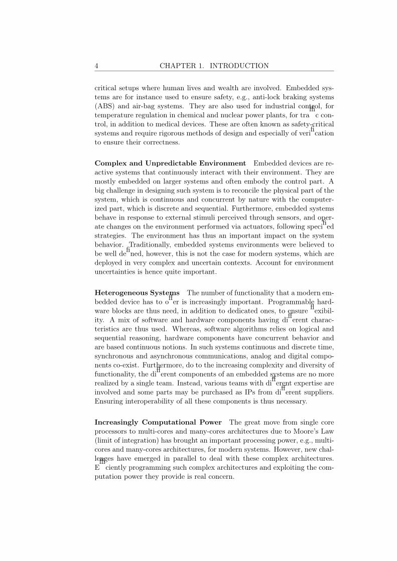
Figure 1.1: The Y-chart Scheme for mapping application to architecture.
CHAPTER 1. INTRODUCTION 7
When building models, separation of concerns is crucial as stipulatedin system-level design. This involves i) the separation of computation andcommunication and ii) the separation of application from the architecture.The latter is particularly useful for the design of programmable systems,where it is required to distinguish the software application from the hardwarearchitecture. Different strategies can be then investigated to map applicationfunctionality to architectures components, which is of great importance inthe context of multi-core or many-cores architectures. This is often describedas the Y-chart [128] method depicted in Figure 1.1. The second separationprincipal has been further developed and extended in the platform-baseddesign approach [184]. This advocates using a parameterizable platform fora class of applications per domain to enhance components reuse and thusproduction and reduce cost.
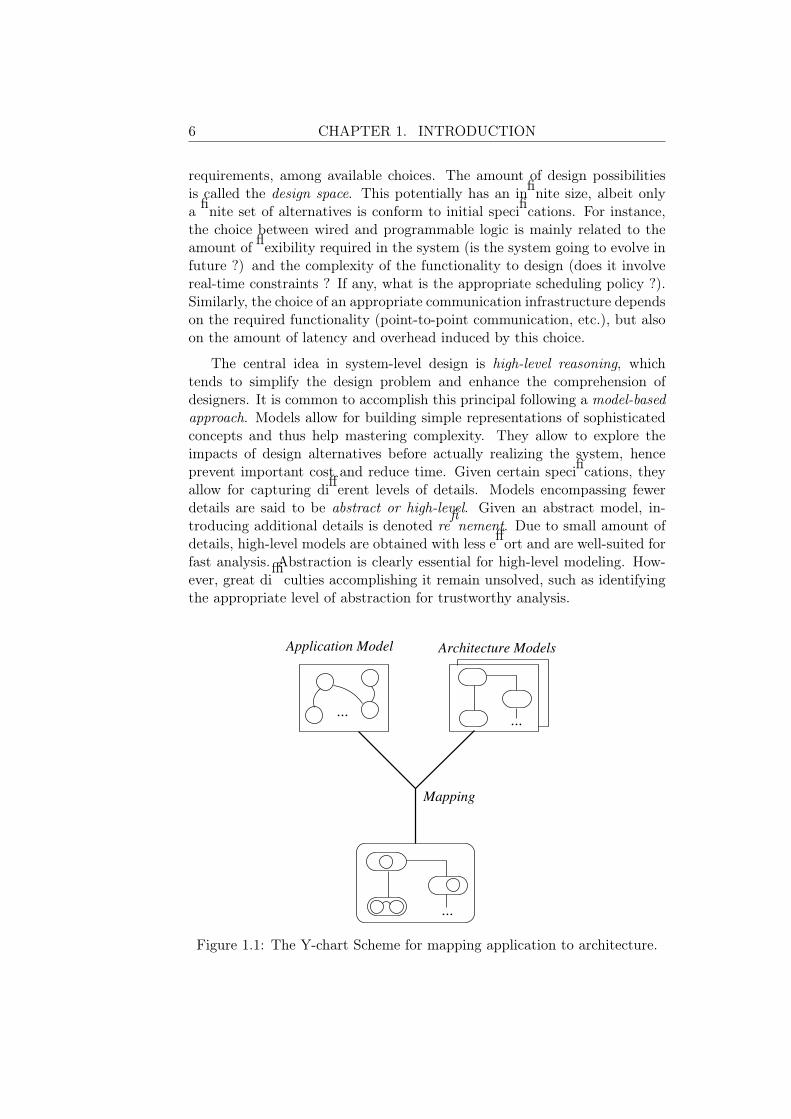
At each step of the design process, making a choice implicitly implies toeliminate alternatives and thus to reduce the design space as illustrated inFigure 1.2. The highest importance in system-level design method is givento the earliest design steps. During these phases, the number of alternativesis the most important, thus decisions have the greatest impact on the rest ofthe process. For instance, bad decisions at this level, may lead to unfeasibledesign or to a design where some requirements cannot be met. SystematicDesign space exploration methods are indispensable to investigate the designalternatives at different phases of the process. Such methods are required tobe fast and accurate to enable well-founded decision at early stages.
Impact
of
Des
ign D
ecis
ions
Initial Specifications
Des
ign T
ime
Lev
el o
f A
bst
ract
ion
Figure 1.2: Schematic view of exploring the design space [197].

8 CHAPTER 1. INTRODUCTION
A generic scheme of design space exploration is presented in figure 1.3. Itconsists of an iterative process repeated for each design phase and potentiallyleading to next design phases. For the earliest phases, given initial specifi-cations, high-level models capturing the main functionality in an abstractway are first built. These models represent different realizations alternativesof functionality of interest. Following the Y-chart pattern, separate modelsof application and architecture are produced. Analysis is then performedon each alternative to check conformance with the given requirements. Theobtained analysis results are essential to decide which alternative is the mostappropriate with respect to functional and extra-functional aspects.
Specifications
Analysis
Modeling
Alternative Models
Investigation Results
Decision
Model
Refinement
Improvements
Figure 1.3: A generic process of design space exploration.
1.2.3 State of the Art
The generic process of design space exploration is widely adopted in sev-eral state-of-the-art tools following system-level design guidelines. For manydecades, embedded systems designers were operating at very low-levels ofabstraction, e.g., transistor-level, gate-level, or register transfer-level (RTL).Due to the increasing complexity and the exponential growth of functionality,rising the level of abstraction has become inevitable. Methods operating athigher-levels such as transaction-level modeling (TLM) [53] or system-levelhave thus emerged.
The shift of embedded systems towards more programmable and flexiblesettings has obliged designers to abandon traditional methodologies pushinginitial specifications, through a sequence of transformations, to a dedicatedwired logic implementation. It is worth to mention that this might still thecase for the design of sub-components of systems.

CHAPTER 1. INTRODUCTION 9
Designing heterogeneous systems encompassing programmable and ded-icated components generally falls within one of three configurations:
1. The first setting concerns architecture exploration, which is for instanceuseful to find the most appropriate architecture for a given domain ofapplication, e.g., multimedia or communication.
2. Another possible configuration is when the architecture is known andthe goal is to design and map software application to this architecture.
3. The third possible setting is the classical co-design situation wheresome functionality specification are given and the aim is to find thebest partition into programmable and dedicated components.
These settings may coexist withing a single design process, e.g., at differentphases of the process, or in independent processes for different applicationdomains.
When confronted with these settings, different design approaches arepossible, mainly in term of potential abstraction choices. For instance, thefirst setting requires to consider various applications in a specific domainthat will constitute a benchmark for architectures exploration. To this end,abstracting functional details of applications is essential to ensure a fast ex-ploration and a maximum of coverage. This is for example the case for theSPADE (System-level Performance Analysis and Design space Exploration)methodology [150], which relies on trace-driven simulation for architectureexploration. Trace-driven simulation consists of transforming models of ap-plications into traces containing coarse-grained computation and communi-cation operations. Similarly, the Artemis Workbench [168] offer the samefunctionality, although not limited to.
Partitioning initial specifications into programmable and dedicated com-ponents is among the most difficult and time consuming design activitiesbecause of the huge number of design alternatives. Only few methodologiesproviding assistance towards this goal exist. This is for instance the caseof the POLIS [17] and the VCC methodologies, which start from high-levelmodels that do not discriminate software and hardware components. An ex-plicit partitioning process is performed to identify candidate components forsoftware implementation. The methodologies were actually proposed in thecontext of automotive industry, often relying on single processor architec-tures. The increasing difficulty to partition functionality into hardware andsoftware components has motivated the emergence of platform-based designapproach [184] where a common denominator architecture is used for a givenapplication domain. Such an architecture may be found using architectureexploration methodologies mentioned above.
The current state of embedded systems design mostly consider potentialtarget architectures in addition to initial specifications, which correspondto the second setting discussed earlier. This may be following a platform-based approach, using human expertise, previous knowledge, or experience.

10 CHAPTER 1. INTRODUCTION
The considered target architecture may be completely specified or allow pa-rameterization, e.g., cache size. In such configuration, embedded softwaredesign become very important. Moreover, with the emergence of multi-coreand many-cores architectures, additional challenges such as finding the bestparallelization and the optimal mapping of the application into architecture,figuring out the best communication mechanism to use, and finding softwarecomponents parameters, e.g., queues size, are real concerns.
Most of the state of the art methodologies provide automated supportto find one or several candidate mappings, generally taking into accountfunctional and performance aspects. In this context, abstraction is moretargeted to the architecture part of the system, although different possibil-ities are proposed in the literature. Several methodologies rely on librariesof generic hardware components at different levels of abstractions. For in-stance, the Artemis Workbench [168], DOL (Distributed Operation Layer)[198], and VISTA [159] use SystemC to model hardware components at dif-ferent abstraction levels. Vista provides cycle-accurate TLM components tobuild virtual SoC architecture, whereas DOL offers high-level components.Artemis is based on the Sesame environment [66, 169] for architecture andapplication modeling. It provides hardware components capturing only per-formance information and not functional behavior. Other methodologiessuch as Metropolis [18] and MILAN [16] are based on meta-models.
Performance aspects are essential to make well-founded decisions in thedifferent discussed settings. Integration of these information within high-level models is quite important for trustworthy design space exploration andconsequently to a successful design.
Besides the important work in industry and academia proposing variousdesign methods, several technical and theoretical problems remain unsolved.For instance, a big challenge in this context is building appropriate abstrac-tions of application and architecture and their combination. Furthermore,performance aspects are still not very well understood, especially at system-level. As depicted in the next section, important challenges remains aheadfor modeling and analyzing them faithfully at system-level.
1.3 Performance in System-level Design
For many years, functional aspects were in the center of system-level de-sign methods, while extra-functional ones were considered as second-classcitizens. Traditionally, ad hoc performance models decorrelated from func-tional behavior, built late in the design process and coupled with simpleanalysis techniques were the unique performance evaluation support.
As stated earlier, in modern systems such as wearable and portable de-vices, where a limited amount of resources is available and an increasingnumber of functionality is required, extra-functional aspects are becoming

CHAPTER 1. INTRODUCTION 11
equally important and not considering them may lead to poor results laterin the design process. For instance, a smartphone that quickly losses energyor a multimedia device with a considerable response time (latency) is notgoing to sell even if it provides all required services. An equally importantissue is to find trade-offs between different extra-functional requirements.For example, selecting a security strategy, involving cryptography, of somedistributed setting which is monitored through portable devices must takeinto account autonomy issues.
Additional requirements concerning the models and the analysis tech-niques to use for system-level design of embedded systems are thereforeneeded. First, building high-level models that only capture the functionalbehavior of the system is no more sufficient. Taking into account extra-functional aspects, especially performance is a must for a successful design,which rises several questions about traditional models and their convenience.Second, given the importance of such aspects for well-founded decisions dur-ing design space exploration, classical performance evaluation techniques areno more sufficient.
While dealing with functional specifications has reached relatively ma-ture state (a large body of theoretical and practical results), we still lackmethods and tools to rigorously and systematically handling extra-functionalrequirements. These remain not well understood and still difficult to han-dle, especially at the earliest design phases. Dealing with these aspects atsystem-level brings additional difficulties which span from the specificationphase to the analysis of the global system.
Our interest is to contribute advancing the state-of-the-art on system-level design. In particular, we aim at conceiving techniques and methods forbetter support of performance requirements following the system-level guide-lines above. We approach this problem by first analyzing the current andsought challenges of dealing with performance at system-level. These chal-lenges will guide us to identify the main requirements for building or usingthe appropriate methods and techniques to achieve our objective. Moreover,based on the previous analysis, we pinpoint modeling and analysis as thetwo main activities of a design process. Thus, in the next section, we willdecompose the identification of requirements into identification of modelingrequirements and identification of analysis requirements.
1.3.1 Challenges
The System Dimension. Because of their weak interaction with thephysical world, classical computer systems are essentially designed basedon strong abstractions of physical artifacts. For instance, building softwareapplications to run on a computer, entails designing an algorithm for whichphysical time and memory complexities are evaluated, using complexity the-ory, with respect to abstract execution models, e.g., Turing machine. Such
12 CHAPTER 1. INTRODUCTION
abstractions are inappropriate for embedded systems because of the tightconnection of the physical and cyber worlds. Performance of embedded sys-tems is strongly related to the physical part of the system, e.g., executionof some functionality by specific architecture components; execution timeof a Fourier transform on a processing unit, communication delay of a busor a Network on Chip (NoC), amount of consumed energy or dissipatedtemperature induced by that function on the corresponding hardware. Thisshift from a program view to a system perspective gave rise to importanttheoretical and technical issues.
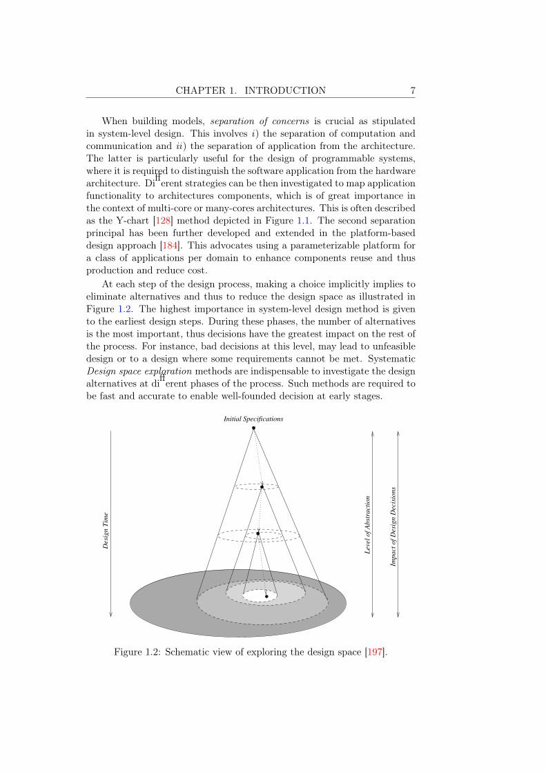
Contradictory Goals, Abstract Vs. Faithful. The modeling activityat system-level aims at enhancing designers comprehension and reducing ef-fort by performing high-level reasoning. Thus, on one hand, one wants todeal with abstract models that minimize the modeling effort and the ex-ploration time. On the other hand, these models are required to captureperformance details in order to precisely reflect the reality and enable ac-curate reasoning about the whole system performance. This highlights theneed of building good abstractions.
Availability in Early Design Phases. Because of the tight connectionbetween cyber and physical worlds, performance aspects of embedded sys-tems cannot be thought of independently of the hardware part of the system.However, the latter are rarely available in early design phases since physicalrealization of the hardware architecture come relatively late in the designprocess. This makes building high-level models encompassing faithful per-formance details quite challenging. Hence, only approximation or estimationof such details at different level of details is possible at system-level.
Variability. Performance details are characterized by their significant vari-ability which obviously cannot be captured by point estimates. This fluc-tuation is mainly due to three reasons. First, the inputs (or the workload)are generally variable, albeit some systems are data-independent, that is,their performance is constant for various input data. Second, the impact ofthe environment, which is often unpredictable, is important. This under-lines robustness requirements of embedded systems. The third reason is theinherent hardware components behavior, e.g., caches, memory contention,arbitration mechanisms, etc. These cannot be captured in details in earlydesign phases because of the lack of detailed specification and the requiredhigh-level of abstraction.
1.3.2 Performance Modeling Requirements
The above challenges rise several natural questions with respect to themodeling process at system-level. The main question one have to answer is
CHAPTER 1. INTRODUCTION 13
How to build high-level models encompassing performance details in additionto functional behavior while ensuring faithfulness ? This question can bedecomposed to several sub-questions that concern, on one hand the modelsto use: i) What is an appropriate characterization of performance details? ii)What is a well-suited model for capturing functional and performance aspectsat system-level? On the other hand, question concerning the process tofollow: iii) How to capture performance information in early design phases?
Let us first consider the first two questions, that is, i) and ii). Gener-ally two types of modeling approaches, providing orthogonal abstractions,exist, namely computational (machine-based, e.g., automata) and analytical(equation-based, e.g., transfer function) [109]. Because their are executable,computational models are often used to describe software systems, while an-alytical ones are more appropriate for hardware, since they capture morenaturally concurrency and quantitative aspects. Whereas analytical modelsare inherently mathematically defined, computational models are not neces-sarily formal. Most of the time, these are obtained using modeling languages(textual or graphical), where the dynamic behavior is not formally specified,e.g., Java threads or Unified Modeling Languages (UML) [182]. Formal com-putational models in contrast, are the result of well-defined modeling lan-guages, that is, with mathematically specified operational semantics, e.g.,Petri nets [179].
In this thesis, a mathematically defined framework defining the seman-tics of a given modeling language is denoted as a formalism. Furthermore,we distinguish modeling languages used to catch systems functionality fromthose used to specify system requirements, e.g., good properties to satisfyor bad properties to avoid, denoted property specification languages. Backto the previous questions, based on the identified challenges, we impose thefollowing constraints on modeling (respectively property specification) lan-guages and system models (respectively system properties) to capture bothfunctional and performance aspects at system-level.
Requirements on Modeling and Property Specification Languages
To deal with the above challenges, it is required to dispose of languagesthat are sufficiently expressive to cover the different aspects of software,hardware, and the interactions between them. These should also have clearsemantics to enable rigorous reasoning and interoperability, in addition toproviding support for quantitative aspects.
Expressiveness is the ability of a languages to provide intuitive, read-able, and succinct mechanisms towards representing the different aspects ofa system. To capture hardware and software aspects, a modeling languageshould provide means to express concurrent as well as sequential behaviors,continuous as well as discrete time, functional and extra-functional aspects.Another important ingredient concerns communications mechanisms which
14 CHAPTER 1. INTRODUCTION
maybe for instance synchronous or asynchronous. Modeling languages shouldalso enable capturing uncertainties and variability through stochastic and/ornon-deterministic support.
A natural way for building artifacts is incrementally and in a composi-tional fashion. The system is seen as a set of actors or components havingcertain behavior and properties which are assembled in a rigorous manner toachieve the global required behavior of the system. This entails component-based modeling languages.
Requirements on Models and Properties
Due to their central role in systems design, models must have clear inter-pretations which leaves no place for ambiguity. Models are hence requiredto be formal, that is, governed by clear semantics free of ambiguity, which isachieved by adopting a certain formalism. Furthermore, a model in system-level design is required to capture only the gist of the system behavior re-quired in the corresponding phase, that is, with respect to taking decisionin that stage or level. In contrast, models should also be faithful in thatthey reflect the real specifications of the system. Furthermore, models arerequired to be executable to enable fast prototyping and analysis.
Requirements on Performance Modeling Methods
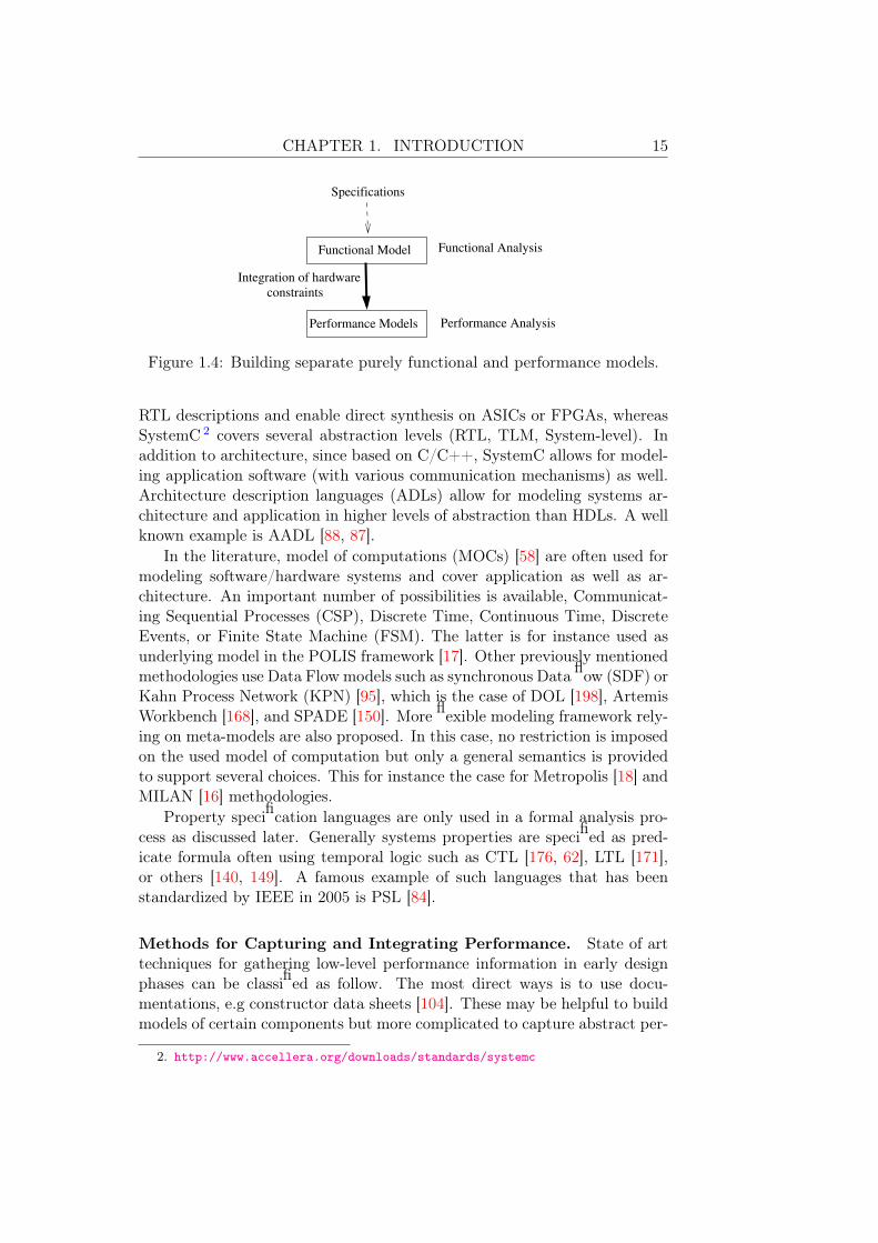
The remaining question from the modeling perspective (iii) concerns theapproach to use in order to capture performance details at system-level.First, it is worth mentioning that since complete physical details cannotbe obtained in early design phases, such approach is expected to performestimation from concrete or low-level hardware descriptions. Second, theused approach should be able to precisely capture performance variabilitywhile still abstract (not too verbose characterization). Finally, such methodshould be automatic (tool-supported) and fast to avoid creating bottlenecksthat will eventually slow down the design space exploration. An importantrequirement is that the method keeps separated purely functional modelsfrom models containing in addition performance information (called perfor-mance models in this work) as shwon in Figure 1.4. This is important inorder to ensure incremental design and separate analysis at different levelsof abstractions.
State of the Art
Modeling and Property Specification Languages. Several represen-tations were proposed in the literature to model application and architecture.The most common for architectures description are hardware descriptionlanguages (HDLs). These enable modeling architecture behavior at differentlevels of abstractions. For example, VHDL and Verilog are often used for
CHAPTER 1. INTRODUCTION 15
Functional Model Functional Analysis
Performance Models Performance Analysis
Integration of hardware
constraints
Specifications
Figure 1.4: Building separate purely functional and performance models.
RTL descriptions and enable direct synthesis on ASICs or FPGAs, whereasSystemC 2 covers several abstraction levels (RTL, TLM, System-level). Inaddition to architecture, since based on C/C++, SystemC allows for model-ing application software (with various communication mechanisms) as well.Architecture description languages (ADLs) allow for modeling systems ar-chitecture and application in higher levels of abstraction than HDLs. A wellknown example is AADL [88, 87].
In the literature, model of computations (MOCs) [58] are often used formodeling software/hardware systems and cover application as well as ar-chitecture. An important number of possibilities is available, Communicat-ing Sequential Processes (CSP), Discrete Time, Continuous Time, DiscreteEvents, or Finite State Machine (FSM). The latter is for instance used asunderlying model in the POLIS framework [17]. Other previously mentionedmethodologies use Data Flow models such as synchronous Data flow (SDF) orKahn Process Network (KPN) [95], which is the case of DOL [198], ArtemisWorkbench [168], and SPADE [150]. More flexible modeling framework rely-ing on meta-models are also proposed. In this case, no restriction is imposedon the used model of computation but only a general semantics is providedto support several choices. This for instance the case for Metropolis [18] andMILAN [16] methodologies.
Property specification languages are only used in a formal analysis pro-cess as discussed later. Generally systems properties are specified as pred-icate formula often using temporal logic such as CTL [176, 62], LTL [171],or others [140, 149]. A famous example of such languages that has beenstandardized by IEEE in 2005 is PSL [84].
Methods for Capturing and Integrating Performance. State of arttechniques for gathering low-level performance information in early designphases can be classified as follow. The most direct ways is to use docu-mentations, e.g constructor data sheets [104]. These may be helpful to buildmodels of certain components but more complicated to capture abstract per-
2. http://www.accellera.org/downloads/standards/systemc

16 CHAPTER 1. INTRODUCTION
formance information, especially their variation. Performance details mayalso be obtained from source/binary/object code, e.g static analysis or codeinspection [45, 23]. This needs a (cross-)compiler and code profiling, al-though does not capture the dynamic behavior of the system. The mostaccurate and the most used technique relies on executable i.e high/low-levelsimulation or execution, albeit it is known to be time and resource consuming[17, 150, 158, 169].
Several frameworks for system-level design uses these techniques togetherwith model calibration to improve the accuracy of high-level models. Modelcalibration, also referred to as back-annotation, is a well-known and widely-used technique which consists of adding specific details to a given model.However, it only received a little attention in the system-level design com-munity and few frameworks consider and implement it in different ways.
In [170], the authors use low-level simulation and synthesis to calibratearchitecture models in the context of the Sesame simulation framework [169].The proposed techniques rely on instruction-set simulator (ISS) to calibrateprogrammable components and on automatic synthesis targeting FPGAs fordedicated ones. The goal is to build latency tables associated with architec-ture components models.
A system-level performance estimation method [158] for the MILANframework [16] is proposed to calibrate parametrizable models of virtualSoC architecture using interpretive simulation techniques. Starting from ini-tial performance values given by the designer, isolated simulation of specificapplication components mapped to specific architecture ones is performed.The obtained measures concern energy and latency and are characterized asaverage estimates. Later on, based on task graph, composite estimate arederived for energy and latency as well.
In the context of the BIP design flow [44], calibration is performed on twophases. First, hardware constraints concerning computation and communi-cation delays are integrated, through refinement, at the level of the systemmodel, that is the result of mapping application models into architecture.Application component are also calibrated with low-level performance de-tails using tow techniques, namely Instruction Weight Tables (static) andPlatform Dependent Code Generation (dynamic).
In [104], an approach is proposed for automatic code generation and cali-bration of compositional performance models. It relies on high and low-levelsimulations in addition to data sheets to obtain components performanceparameters which are mainly used to characterize arrival and service curvesin term of best-case and worst case execution time (WCET) since relying onReal Time Calculus [199].
An improvement of the VCC methodology using back-annotation of high-level behavioral models is proposed in [96]. Performance estimation is per-formed using statistical approach but only consider a single microprocessor.More specifically, the approach is based on linear regression analysis tech-
CHAPTER 1. INTRODUCTION 17
niques. Similarly, Scope [3] uses statistical regression analysis to performpower estimation of co-processors.
It is worth to observe that different performance estimation and calibra-tion approaches provides completely different abstractions. Besides the levelof detail of the initial models, the characterization approach of performancedetails (the type of the obtained characterization), the choice to calibrate ei-ther application or architecture models or both, and the decision to considerone or both models during the mapping step potentially produce differentsystem model which might be appropriate for different design phases.
1.3.3 Performance Evaluation Requirements
Analysis of models encompassing functional and extra-functional, soft-ware and hardware aspects is challenging in different senses. Assuming thatsuch models are already built, their size is expected to be important. Inspite of the software and hardware aspects of real-life systems, formal mod-els are often heavier to explore. Thus scalability is a real issue, especiallywhen using rigorous analysis techniques. Analysis should not be intrusiveto not alter the correct behavior of the model under analysis. The level ofrequired abstraction for system-level analysis should be carefully chosen tonot mask the relevant details for analysis. It is important that the usedanalysis technique provide quantitative results of performance. Moreoverit should report accurate results, that is, approximation not too far fromreality. Another important requirement about performance evaluation tech-niques is that they have to be fast to enable several analysis iterations inorder to cover a maximum of design alternatives.
State of the Art
State-of-the-art performance analysis techniques at system-level can bebroadly divided in two general families, pure simulation-based and formalapproaches. Nonetheless, some works propose to combine techniques fromboth groups towards hybrid approaches.
Pure simulation-based techniques enable to simulate system components,e.g., independent hardware and software, or to co-simulate both parts at dif-ferent abstraction levels: cycle-accurate using instruction-set simulator (ISS)for instance or higher levels such as functional simulations. Industrial toolsoften rely on simulation techniques for performance analysis, for instance,Seamless Hw/Sw Co-verification 3 or Synopsis System Studio 4. Academicmethodologies mostly base their performance analysis on simulation as well.
3. http://www.mentor.com/products/fv/seamless/
4. http://www.synopsys.com/Systems/BlockDesign/DigitalSignalProcessing/
Pages/SystemStudio.aspx

18 CHAPTER 1. INTRODUCTION
This is for example the case of Artemis Workbench [168], SPADE [150], MI-LAN [16], and Metropolis [18]. Simulation-based approaches mainly sufferfrom long run-time and coverage issues. Some of the above methodologiespropose trace-driven techniques to remedy to long simulation, which useco-simulation to build abstract event traces that are later used for lighteranalysis such as in the Artemis Workbench and SPADE.
To deal with the increasing complexity and the critical aspects of modernembedded systems, it is required to rigorously verify that the built systemmatches the given specifications and requirements. Traditional methods con-sist mainly of testing and peer reviewing of code, which are widely used inindustry 5 and are able to capture a wide class of errors. However, theysuffer from several disadvantages such as manual or semi-automated proce-dures, coverage issues, and more importantly, they can only detect presenceof errors and not their absence. Formal methods provide an automated alter-native for system verification. Moreover, they offer mathematical guaranteesfor the absence (respectively presence) of a bad behavior (respectively goodbehavior). Formal methods for performance analysis can be classified intotow main categories with respect to the used formal models, namely basedon computational models or on analytical ones.
Analytical-based. They mainly rely on the Real Time Calculus (RTC)method [199], which respectively characterizes workload and processingpower as arrival and service curves. Arrival curves for example, captureupper and lower bounds of arrival time of a class of events. RTC wasadopted and extended in several researches such as SymTA/S [107],MAST [100], and modular performance analysis (MPA) [55]. The latteris used within the DOL methodology [198] for system-level performanceanalysis. These methods are actually conceived to be constrained andoften used to compute worst case scenarios.
Computational-based. They are primarily based on model checking (MC)[176, 62], which is a verification method that considers a formal modelM of a system and formal representation of a requirement φ, andanswers the question if M satisfies φ. As illustrated in Figure 1.5, itprovides a yes or no answer and, when the property is not satisfied, itgives a counter-example as a witness. The model checking techniquesexploits the formal definition of the inputs, i.e., M and φ, to performsystematic and exhaustive analysis. Given M and φ formalism, everystate of M might be verified to satisfy or not φ. Exhaustive analysisconstitutes the main limitation of MC techniques since it implies anexponential exploration, known as state-space explosion. Despite theiradvantages, MC methods are still difficult to achieve and hence not yetwidely adopted, especially, for performance analysis. MetaMoc [69] is
5. For instance, between 30% and 50% of the total cost of software development isallocated to testing [15].
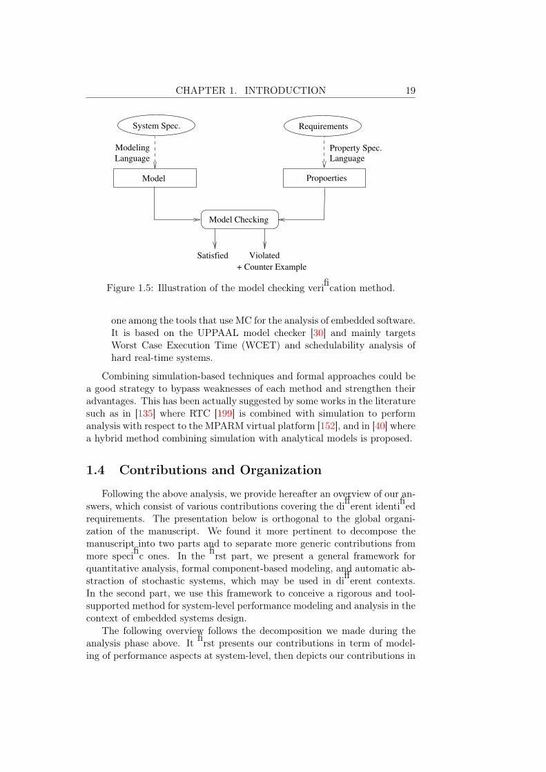
CHAPTER 1. INTRODUCTION 19
Model Propoerties
Model Checking
Language
Modeling Property Spec.
Language
System Spec.
Satisfied Violated
+ Counter Example
Requirements
Figure 1.5: Illustration of the model checking verification method.
one among the tools that use MC for the analysis of embedded software.It is based on the UPPAAL model checker [30] and mainly targetsWorst Case Execution Time (WCET) and schedulability analysis ofhard real-time systems.
Combining simulation-based techniques and formal approaches could bea good strategy to bypass weaknesses of each method and strengthen theiradvantages. This has been actually suggested by some works in the literaturesuch as in [135] where RTC [199] is combined with simulation to performanalysis with respect to the MPARM virtual platform [152], and in [40] wherea hybrid method combining simulation with analytical models is proposed.
1.4 Contributions and Organization
Following the above analysis, we provide hereafter an overview of our an-swers, which consist of various contributions covering the different identifiedrequirements. The presentation below is orthogonal to the global organi-zation of the manuscript. We found it more pertinent to decompose themanuscript into two parts and to separate more generic contributions frommore specific ones. In the first part, we present a general framework forquantitative analysis, formal component-based modeling, and automatic ab-straction of stochastic systems, which may be used in different contexts.In the second part, we use this framework to conceive a rigorous and tool-supported method for system-level performance modeling and analysis in thecontext of embedded systems design.
The following overview follows the decomposition we made during theanalysis phase above. It first presents our contributions in term of model-ing of performance aspects at system-level, then depicts our contributions in

20 CHAPTER 1. INTRODUCTION
performance evaluation. Finally, it illustrates our global answer to the iden-tified requirements, which is a rigorous, systematic and integrated methodfor performance modeling and analysis for systems-level design of embeddedsystems, called ASTROLABE. We opted for such a double decomposition tomatch our answers with the above identified requirements and to facilitatereading the manuscript.
1.4.1 System-level Modeling
Stochastic Component-based Formalism
We propose a component-based modeling language to handle system com-plexity. This is based on the BIP framework [28], which enables incrementalsystem design starting from simple components which are later assembledtogether to build more complex functionality. This approach enables compo-nents reuse, hence reduces modeling time and enhance productivity. BIP hasa well defined semantics for components modeling (behavior and interfaces)and for specifying coordination between them. It offers different communi-cation mechanisms that are shown to be sufficiently expressive and enablesuser-defined scheduling policies. Moreover, BIP supports different timingmodels in addition to well-defined real-time semantics.
Our main contribution at this level, is the extension of this framework tosupport stochastic systems modeling. We mainly provide a syntactic exten-sion of the language to enable modeling probabilistic behavior and a formalspecification of the operational semantics of stochastic behavior. As we willexpose in Chapter 3, the proposed stochastic component-based formalismdenoted SBIP, is shown to be well suited to model functional as well asperformance aspects. The latter are captured as probability distributionsor more sophisticated probabilistic models. The semantics of SBIP, is suffi-ciently expressive to be used as single semantics driving the different designphases and to separately capture software and hardware models.
Code Generation
To enable gathering accurate performance information in early designphases, we rely on automatic code generation. Starting from applicationfunctional models, we generate concrete implementations targeting low-levelmodels of architecture: virtual prototype, or physical implementation (FPGAor final chip), depending on the design phase. This enable accurate (sincebased on concrete execution) yet fast (automatic generation of implemen-tation and deployment code) prototyping as shown in Chapter 5. Thisentails instrumentation of performance dimensions (time, energy, temper-ature, memory) of interest (obtained from systems requirements) and perti-nent functionality to measure. Automatic code generation produces parallel

CHAPTER 1. INTRODUCTION 21
implementations for many-cores platforms, which answer the increasing com-plexity of programming these architecture challenges. An implementation ofa code generator targeting the STHORM platform [155] by STMicroelec-tronics is presented in Chapter 7.
Statistical Characterization of Performance
To faithfully characterize performance details, we propose to use auto-matic learning techniques from concrete executions. This enables to capturethe real performance characteristics of the application running on specificarchitecture with respect to some portioning. Moreover, we suggest learn-ing probabilistic models of performance, e.g., probability distributions, tocorrectly catch variability. We believe that such models provide good ab-straction of physical details without losing the gist. In Chapter 6, we detailhow we use statistical inference algorithms to build such probabilistic per-formance characterizations. In Chapter 7, we provide tool support for thestatistical inference procedure.
Model Calibration
The method we propose to build faithful performance models is to cal-ibrate functional models (application and architecture), which are timelessand does not contain any information about energy consumption or temper-ature for instance, with probabilistic characterizations of performance. Thisback-annotation mechanism will produce stochastic models encompassingthe functional behavior of the system in addition to the performance aspectsat a good level of abstraction, that is appropriate for the earliest explorationphases as we will detail in Chapter 5.
1.4.2 System-level Verification
Performance Analysis
Our contribution at this level is to use a formal verification technique,namely statistical model checking (SMC) [110, 209], introduced in Chapter 2.Our proposal is a trade-off between purely simulation-based methods andanalytical techniques, which consists of stochastic (Monte-Carlo) simulationand statistical tests. It combines benefits of both approaches, that is, thespeed of simulation and the well-founded of analytical approaches. SMC onlyprovides approximations which can be controlled by using user-defined levelof confidence. Moreover, it allows for quantitative results, which are moreappropriate for performance evaluation. To the best of our knowledge, thisis the first time SMC is being used for performance evaluation of embeddedsystems. A second contribution in this context is the implementation of theBIPSMC statistical model checker presented in Chapter 7.
22 CHAPTER 1. INTRODUCTION
Automatic Stochastic Abstraction
To answer the issues induced by analysis of software/hardware models(the important size of the model) and the challenges of performing specifi-cally formal verification (state space explosion, important time), we proposein Chapter 4, a technique for automatically building models abstraction. Ouridea is to perform abstraction with respect the property we want to verify onthe model. The proposed technique is based on machine learning algorithmsand enables to learn an abstraction from execution traces even in case ofblack-box models.
1.4.3 Integrated Performance Modeling and Analysis
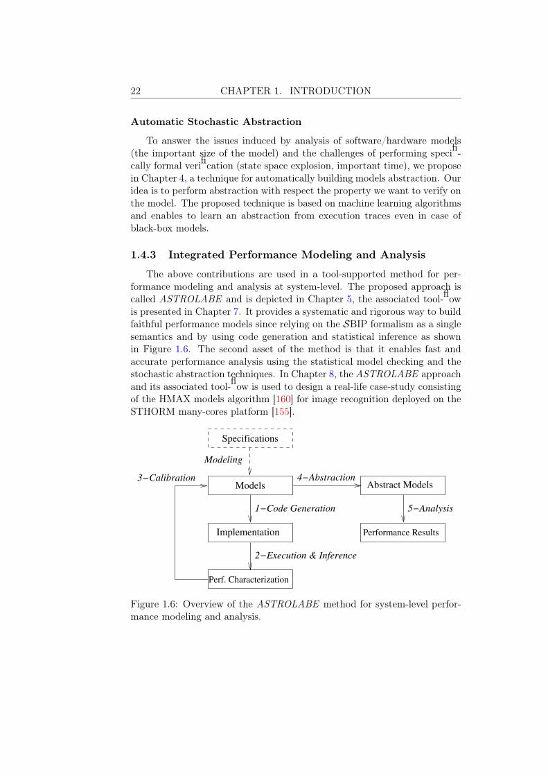
The above contributions are used in a tool-supported method for per-formance modeling and analysis at system-level. The proposed approach iscalled ASTROLABE and is depicted in Chapter 5, the associated tool-flowis presented in Chapter 7. It provides a systematic and rigorous way to buildfaithful performance models since relying on the SBIP formalism as a singlesemantics and by using code generation and statistical inference as shownin Figure 1.6. The second asset of the method is that it enables fast andaccurate performance analysis using the statistical model checking and thestochastic abstraction techniques. In Chapter 8, the ASTROLABE approachand its associated tool-flow is used to design a real-life case-study consistingof the HMAX models algorithm [160] for image recognition deployed on theSTHORM many-cores platform [155].
Specifications
Modeling
Perf. Characterization
4−AbstractionAbstract Models
Performance ResultsImplementation
Models3−Calibration
1−Code Generation
2−Execution & Inference
5−Analysis
Figure 1.6: Overview of the ASTROLABE method for system-level perfor-mance modeling and analysis.

PART I
FORMALISMS AND
TECHNIQUES
23


Chapter 2Quantitative Analysis of Stochastic
Models: A Background
In this first part of the thesis, we aim at providing a theoretical foun-dation upon which we will build our method for system-level performancemodeling and analysis for many-cores embedded systems. We propose a setof formalisms and techniques for stochastic modeling and performance anal-ysis at a high-level of abstraction. The part is composed of three chapters,where the first recalls general formalisms for stochastic systems modelingand probabilistic requirements specification. It also presents quantitativetechniques for analyzing stochastic systems. In the second chapter, we in-troduce a component-based formalism for modeling stochastic systems anddiscuss its semantics and expressiveness. The third and last chapter of thisfirst part is about abstraction of stochastic models. There, we propose atechnique based on machine learning to automatically build abstract modelsin order to improve scalability and reduce analysis time.
Modeling performance requires rich formalisms that allow for capturingin the same time sophisticated functional behavior and complex performanceinformation. In the context of embedded systems, modeling formalisms areeven more important because of the inherent nature of these systems whichevolve in unpredictable environments, are subject to unexpected situations,hence encompassing a high degree of uncertainty. Stochastic or probabilisticformalisms are thus needed to correctly and faithfully capture these behav-iors. On the other hand, analyzing these models rigorously and efficientlyis a challenging task due to the increasing complexity of modern systems.Quantitative analysis is even more difficult and less understood than classi-cal qualitative analysis techniques. While several techniques exist, we stillencounter difficulties performing such analysis especially at system-level.
This chapter recalls the main concepts of quantitative analysis of stochas-tic models following the model checking approach as stated in the introduc-
25

26CHAPTER 2. QUANTITATIVE ANALYSIS OF STOCHASTIC
MODELS: A BACKGROUND
tion. It first recalls general stochastic modeling formalisms, namely MarkovChains and Markov Decision Processes. It then presents the Linear-timeTemporal Logic and its probabilistic bounded variant as a mean for for-malizing systems requirements. Finally, it introduces the Statistical ModelChecking techniques for analysis of stochastic system models.
Throughout this dissertation, we will adopt a state-based view of stochas-tic processes unless differently stated. Classically, these are seen as sequencesof random variables evolving over time. Moreover, we will only consider finiteand discrete Markov models, i.e., Discrete Time Markov Chains (DTMCs)and Markov Decision Processes (MDPs) and do not discuss continuous timemodels such as Continuous Time Markov Chains (CTMCs). It is worthrecalling that the state-based representation of stochastic processes entailstwo type of labeling, over states and over actions, as we will show alloverthe chapter. As a consequence, the notion of non-determinism may havedifferent meanings accordingly, i.e., we may have non-determinism with re-spect to state labels or with respect to action labels. In this work, we aredefining DTMCs to be only state labeled. Therefore, they are only con-cerned with non-deterministic state labels. In contrast, MDPs are assumedto have labels on both states and actions. Nonetheless, we will only considernon-deterministic actions as we will explain hereafter.
2.1 Stochastic Systems Modeling
We begin by giving a general background on stochastic models. Wefocus on a specific class of models called Markov Models. These have theparticularity to be memoryless, that is, at each time, the decision to moveto a next state only depends on the current state and does not take intoaccount the whole history of the system evolution. We provide hereafter anoverview of two well-known models, namely Discrete Time Markov Chainsand more general ones called Markov Decision Processes which encompassnon-determinism in addition to probabilistic behavior.
Let AP be a finite set of atomic propositions. We define the alphabetΣ = 2AP and denote the elements of Σ (all subsets of AP ) as symbols. Theempty symbol is denoted by τ . As usual, we denote by Σω (respectively byΣ∗) the sets of infinite (respectively finite) words over Σ.
2.1.1 Discrete Time Markov Chains
Along the dissertation, we will use state-labeled Markov Chain, abbrevi-ated to LMC to refer to Discrete Time Markov Chain (DTMC). The readermay find both notations.
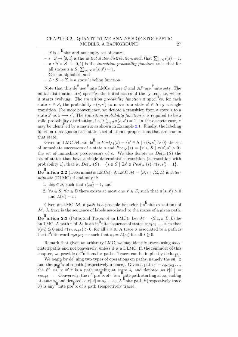
Definition 2.1 (state-Labeled Markov Chain). A state-Labeled MarkovChain M is a tuple �S, ι,π,Σ, L� where,
CHAPTER 2. QUANTITATIVE ANALYSIS OF STOCHASTICMODELS: A BACKGROUND 27
– S is a finite and nonempty set of states,– ι : S → [0, 1] is the initial states distribution, such that
�s∈S ι(s) = 1,
– π : S × S → [0, 1] is the transition probability function, such that forall states s ∈ S,
�s�∈S π(s, s�) = 1,
– Σ is an alphabet, and– L : S → Σ is a state labeling function.
Note that this defines finite LMCs where S and AP are finite sets. Theinitial distribution ι(s) specifies the initial states of the system, i.e, whereit starts evolving. The transition probability function π specifies, for eachstate s ∈ S, the probability π(s, s�) to move to a state s� ∈ S by a singletransition. For more convenience, we denote a transition from a state s to astate s� as s −→ s�. The transition probability function π is required to be avalid probability distribution, i.e,
�s�∈S π(s, s�) = 1. In the discrete case, π
may be identified by a matrix as shown in Example 2.1. Finally, the labelingfunction L assigns to each state a set of atomic propositions that are true inthat state.
Given an LMC M, we define PostM(s) = {s� ∈ S | π(s, s�) > 0} the setof immediate successors of a state s and PreM(s) = {s� ∈ S | π(s�, s) > 0}the set of immediate predecessors of s. We also denote as DetM(S) theset of states that have a single deterministic transition (a transition withprobability 1), that is, DetM(S) = {s ∈ S | ∃s� ∈ PostM(s),π(s, s�) = 1}.Definition 2.2 (Deterministic LMCs). A LMC M = �S, ι,π,Σ, L� is deter-ministic (DLMC) if and only if:
1. ∃s0 ∈ S, such that ι(s0) = 1, and
2. ∀s ∈ S, ∀σ ∈ Σ there exists at most one s� ∈ S, such that π(s, s�) > 0and L(s�) = σ.
Given an LMC M, a path is a possible behavior (infinite execution) ofM. A trace is the sequence of labels associated to the states of a given path.
Definition 2.3 (Paths and Traces of an LMC). Let M = �S, ι,π,Σ, L� bean LMC. A path r of M is an infinite sequence of states s0s1s2 . . . such thatι(s0) > 0 and π(si, si+1) > 0, for all i ≥ 0. A trace σ associated to a path isthe infinite word σ0σ1σ2 . . . such that σi = L(si) for all i ≥ 0.
Remark that given an arbitrary LMC, we may identify traces using asso-ciated paths and not conversely, unless it is a DLMC. In the reminder of thischapter, we provide definitions for paths. Traces can be implicitly deduced.
We begin by defining two types of operations on paths, namely the suffixand the prefix of a path (respectively a trace). Given a path r = s0s1s2 . . .,the ith suffix of r is a path starting at state si and denoted as r[i..] =sisi+1 . . . . Conversely, the ith prefix of r is a finite path starting at s0, endingat state si, and denoted as r[..i] = s0 . . . si. A finite path r̂ (respectively traceσ̂) is any finite prefix of a path (respectively trace).

28CHAPTER 2. QUANTITATIVE ANALYSIS OF STOCHASTIC
MODELS: A BACKGROUND
We denote by Paths(M) (respectively Traces(M)) the set of all in-finite paths (respectively traces) in M and by Pathsfin(M) (respectivelyTracesfin(M)) the set of all finite paths (respectively traces) in M.
Probability Measure of a Markov Chain
The first motivation of building such rich models is to be able to questionthem to get valuable quantitative answers, that is probabilities of relevantevents, e.g., the probability to reach a good state or to avoid a bad state. Tothis end, such models have to be associated with a well defined probabilityspace which is basically a σ-algebra equipped with a probability measure(see [15] for a detailed description of this notions).
In order to define a probability space for a given LMC M, we first needto specify a σ-algebra for it. In the literature, we generally consider theσ-algebra generated by the cylinder sets each consisting of infinite pathsr ∈ Paths(M) having a common prefix, i.e a finite path r̂ ∈ Pathsfin(M).
Definition 2.4 (Cylinder Set of an LMC). The cylinder set of r̂ = s0 . . . sn ∈Pathsfin(M) is Cyl(r̂) = {r ∈ Paths(M) | ∃i ∈ [0, n], where r[..i] = r̂}.
Definition 2.5. The σ-algebra associated with an LMC M is the smallestσ-algebra encompassing all the cylinder sets Cyl(r̂) for all r̂ ∈ Pathsfin(M).This induces a unique probability measure PM on the σ-algebra of M wherethe probabilities of the cylinder sets are as follows. Given r̂ = s0 . . . sn ∈Pathsfin(M),
PM(Cyl(r̂)) = ι(s0) ·�
0≤i<n
π(si, si+1).
Two LMCs M1 and M2 are said to be equivalent, denoted M1 ≈ M2,if they have identical probability measures on all the traces, that is, PM1 =PM2 (see [83] for more details).
Example 2.1. We consider the Craps Gambling Game introduced in [15].In this game, a player starts by rolling two fair six-sided dice. The outcomeof the two dice determines whether he wins or not. If the outcome is 7 or 11,the player wins. If the outcome is 2, 3, or 12, the player looses. Otherwise,the dice are rolled again taking into account the previous outcome (calledpoint). If the new outcome is 7, the player looses. If it is equal to point,he wins. For any other outcome, the dice are rolled again and the processcontinues until the player wins or looses.
The behavior of the craps gambling game is captured by an LMC M. Wegraphically illustrate the corresponding model in Figure 2.1. A possible pathof M is r = s0s1s1s
ω7 ∈ Paths(M), where the player wins after three trials.
The associated trace σ with r is start point4 point4 wonω ∈ Traces(M). Letr̂ =start point4 be a finite path of M. The cylinder set of r̂ is Cyl(r̂) = {start
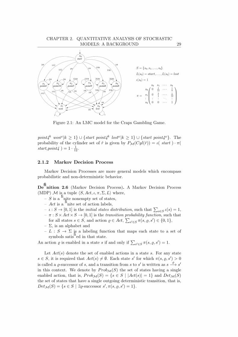
CHAPTER 2. QUANTITATIVE ANALYSIS OF STOCHASTICMODELS: A BACKGROUND 29
won
1/12
1/12
3/4 3/4 13/18 13/18 25/36
1/95/36
5/36
1/92/9
25/36
1/9
1/12
1/121/6
1/91/6
5/36
1/6
1/91/6
5/36
1/6
1 1
1/6
start
point4 point10 point5 point9 point6 point8
lost
s0
s1 s2 s3 s4 s5 s6
s8s7
π =
s0 s1 · · · s8s0 0 1
12 · · · 19
s1 0 34 · · · 1
12.
.
.
.
.
.
.
.
.
.
.
.
.
.
.
s8 0 0 · · · 1
ι(s0) = 1
S = {s0, s1, , ..., s8}L(s0) = start, . . . , L(s8) = lost
Figure 2.1: An LMC model for the Craps Gambling Game.
point4k wonω|k ≥ 1} ∪ {start point4k lostω|k ≥ 1} ∪ {start point4ω}. Theprobability of the cylinder set of r̂ is given by PM(Cyl(r̂)) = ι( start ) · π(start,point4 ) = 1 · 1
12 .
2.1.2 Markov Decision Process
Markov Decision Processes are more general models which encompassprobabilistic and non-deterministic behavior.
Definition 2.6 (Markov Decision Process). A Markov Decision Process(MDP) M is a tuple �S,Act, ι,π,Σ, L� where,
– S is a finite nonempty set of states,– Act is a finite set of action labels,– ι : S → [0, 1] is the initial states distribution, such that
�s∈S ι(s) = 1,
– π : S×Act×S → [0, 1] is the transition probability function, such thatfor all states s ∈ S, and action � ∈ Act,
�s�∈S π(s, �, s�) ∈ {0, 1},
– Σ, is an alphabet and– L : S → Σ is a labeling function that maps each state to a set of
symbols satisfied in that state.
An action � is enabled in a state s if and only if�
s�∈S π(s, �, s�) = 1.
Let Act(s) denote the set of enabled actions in a state s. For any states ∈ S, it is required that Act(s) �= ∅. Each state s� for which π(s, �, s�) > 0
is called a �-successor of s, and a transition from s to s� is written as s�−→ s�
in this context. We denote by ProbM(S) the set of states having a singleenabled action, that is, ProbM(S) = {s ∈ S | |Act(s)| = 1} and DetM(S)the set of states that have a single outgoing deterministic transition, that is,DetM(S) = {s ∈ S | ∃�-successor s�,π(s, �, s�) = 1}.

30CHAPTER 2. QUANTITATIVE ANALYSIS OF STOCHASTIC
MODELS: A BACKGROUND
Intuitively, the behavior of an MDP is as follow. Given ι the initialdistribution, we probabilistically select an initial state s0
1. To move fromstate s0 to some other state, we have first to choose non-deterministicallybetween enabled actions in Act(s0). Once the non-deterministic choice istaken, say � ∈ Act(s0) has been selected, one of the �-successor of s0 isprobabilistically selected according to the distribution π(s0, �, .), where “.”stands for any �-successor from s0.
Example 2.2 (Example of an MDP). Consider the MDP depicted in Fig-ure 2.2 where S = {s0, s1, s2} and s0 is the unique initial state, that isι(s0) = 1. The set of enabled actions are Act(s0) = {�, ς}, Act(s1) =Act(s2) = {ϑ} with respective probabilities, π(s0, �, s1) = 2
3 ,π(s0, �, s0) =13 ,π(s0, ς, s1) = π(s0, ς, s2) = 1
2 ,π(s1,ϑ, s1) = π(s2,ϑ, s0) = 1. In this ex-ample, non-determinism exists between actions � and ς in s0. Remark thatwhatever the choice made between these actions, s1 is reached with a non-null probability.
�, 23ς, 12
ς, 12ϑ, 1�, 13
s1s2 s0ϑ, 1
Figure 2.2: An MDP example.
Similarly to LMCs, a path of an MDP is a potential behavior. How-ever, in this case, it consists of an alternating sequence of states and actionsobtained by performing non-deterministic choices over actions followed byprobabilistic choices over successors.
Definition 2.7 (Paths and Traces of an MDP). Let M = �S,Act, ι,π,Σ, L�be an MDP. A path of M is an infinite alternating sequence of states andactions r = s0�1s1�2s2... such that ι(s0) > 0 and π(si−1, �i, si) > 0 forall i ≥ 0. A trace σ associated to a run s0�1s1�2s2... is the infinite wordL(s0)�1L(s1)�2L(s2).... A finite path (respectively a finite trace) is anyfinite prefix of a path (respectively of a trace). We denote by Paths(M)(respectively Traces(M)) the set of all infinite paths (respectively traces)in M and by Pathsfin(M) (respectively Tracesfin(M)) the set of all finitepaths (respectively traces) in M.
1. In the literature, we may find more general MDP models where several initial dis-tributions are used. In such cases, a non-deterministic choice is performed to select whichinitial distribution to use. For the sake of simplicity, we restrict ourselves to one initialdistribution.
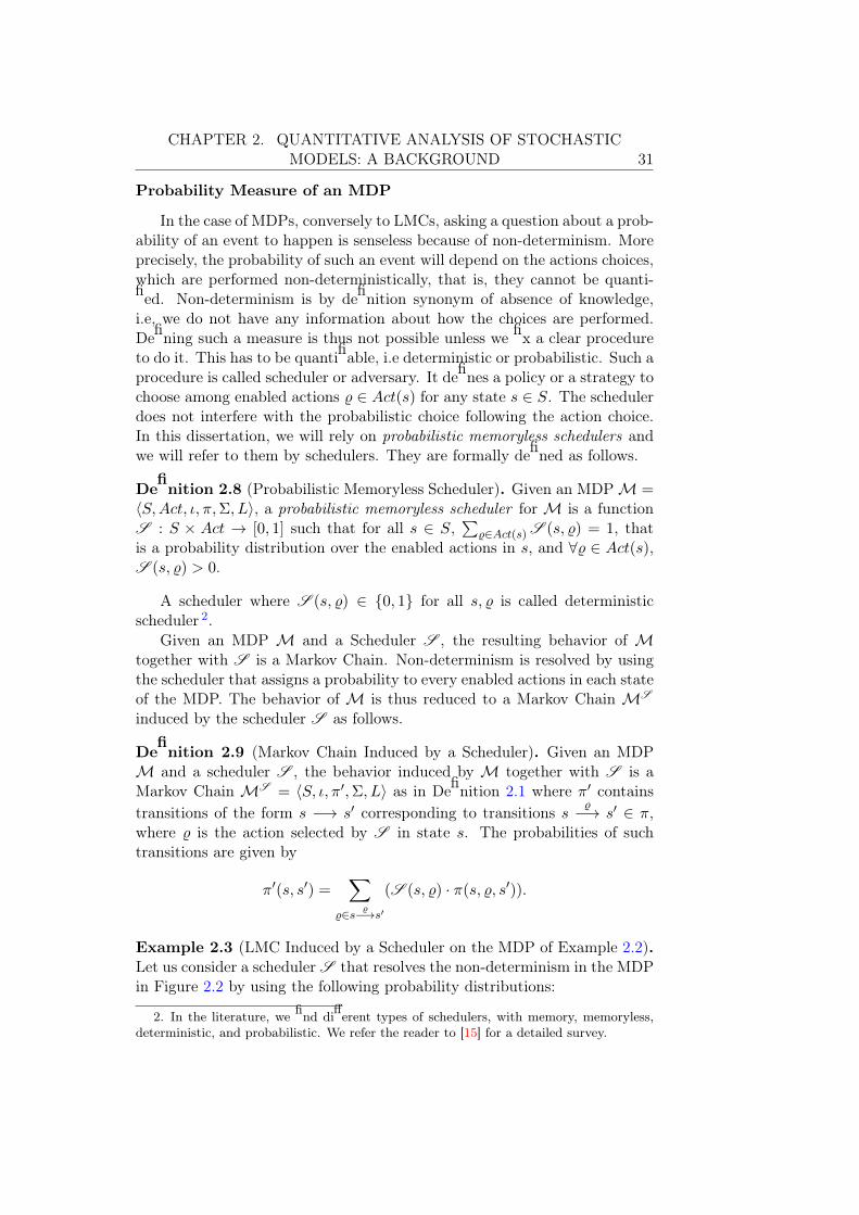
CHAPTER 2. QUANTITATIVE ANALYSIS OF STOCHASTICMODELS: A BACKGROUND 31
Probability Measure of an MDP
In the case of MDPs, conversely to LMCs, asking a question about a prob-ability of an event to happen is senseless because of non-determinism. Moreprecisely, the probability of such an event will depend on the actions choices,which are performed non-deterministically, that is, they cannot be quanti-fied. Non-determinism is by definition synonym of absence of knowledge,i.e, we do not have any information about how the choices are performed.Defining such a measure is thus not possible unless we fix a clear procedureto do it. This has to be quantifiable, i.e deterministic or probabilistic. Such aprocedure is called scheduler or adversary. It defines a policy or a strategy tochoose among enabled actions � ∈ Act(s) for any state s ∈ S. The schedulerdoes not interfere with the probabilistic choice following the action choice.In this dissertation, we will rely on probabilistic memoryless schedulers andwe will refer to them by schedulers. They are formally defined as follows.
Definition 2.8 (Probabilistic Memoryless Scheduler). Given an MDP M =�S,Act, ι,π,Σ, L�, a probabilistic memoryless scheduler for M is a functionS : S × Act → [0, 1] such that for all s ∈ S,
��∈Act(s) S (s, �) = 1, that
is a probability distribution over the enabled actions in s, and ∀� ∈ Act(s),S (s, �) > 0.
A scheduler where S (s, �) ∈ {0, 1} for all s, � is called deterministicscheduler 2.
Given an MDP M and a Scheduler S , the resulting behavior of Mtogether with S is a Markov Chain. Non-determinism is resolved by usingthe scheduler that assigns a probability to every enabled actions in each stateof the MDP. The behavior of M is thus reduced to a Markov Chain MS
induced by the scheduler S as follows.
Definition 2.9 (Markov Chain Induced by a Scheduler). Given an MDPM and a scheduler S , the behavior induced by M together with S is aMarkov Chain MS = �S, ι,π�,Σ, L� as in Definition 2.1 where π� contains
transitions of the form s −→ s� corresponding to transitions s�−→ s� ∈ π,
where � is the action selected by S in state s. The probabilities of suchtransitions are given by
π�(s, s�) =�
�∈s �−→s�
(S (s, �) · π(s, �, s�)).
Example 2.3 (LMC Induced by a Scheduler on the MDP of Example 2.2).Let us consider a scheduler S that resolves the non-determinism in the MDPin Figure 2.2 by using the following probability distributions:
2. In the literature, we find different types of schedulers, with memory, memoryless,deterministic, and probabilistic. We refer the reader to [15] for a detailed survey.
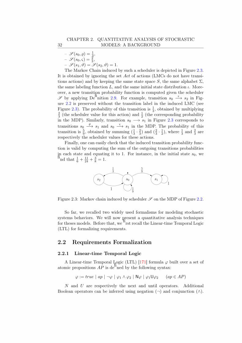
32CHAPTER 2. QUANTITATIVE ANALYSIS OF STOCHASTIC
MODELS: A BACKGROUND
– S (s0, �) =13 ,
– S (s0, ς) =23 ,
– S (s1,ϑ) = S (s2,ϑ) = 1.The Markov Chain induced by such a scheduler is depicted in Figure 2.3.
It is obtained by ignoring the set Act of actions (LMCs do not have transi-tions actions) and by keeping the same state space S, the same alphabet Σ,the same labeling function L, and the same initial state distribution ι. More-over, a new transition probability function is computed given the schedulerS by applying Definition 2.9. For example, transition s0
ς−→ s2 in Fig-ure 2.2 is preserved without the transition label in the induced LMC (seeFigure 2.3). The probability of this transition is 1
3 , obtained by multiplying23 (the scheduler value for this action) and 1
2 (the corresponding probabilityin the MDP). Similarly, transition s0 −→ s1 in Figure 2.3 corresponds to
transitions s0�−→ s1 and s0
ς−→ s1 in the MDP. The probability of thistransition is 5
9 , obtained by summing (13 · 23) and (23 · 1
2), where 13 and 2
3 arerespectively the scheduler values for these actions.
Finally, one can easily check that the induced transition probability func-tion is valid by computing the sum of the outgoing transitions probabilitiesin each state and equating it to 1. For instance, in the initial state s0, wefind that 1
6 + 1124 + 3
8 = 1.
s1s2 s01
19
13
59
1
Figure 2.3: Markov chain induced by scheduler S on the MDP of Figure 2.2.
So far, we recalled two widely used formalisms for modeling stochasticsystems behaviors. We will now present a quantitative analysis techniquesfor theses models. Before that, we first recall the Linear-time Temporal Logic(LTL) for formalizing requirements.
2.2 Requirements Formalization
2.2.1 Linear-time Temporal Logic
A Linear-time Temporal Logic (LTL) [171] formula ϕ built over a set ofatomic propositions AP is defined by the following syntax:
ϕ := true | ap | ¬ϕ | ϕ1 ∧ ϕ2 | Nϕ | ϕ1Uϕ2 (ap ∈ AP )
N and U are respectively the next and until operators. AdditionalBoolean operators can be inferred using negation (¬) and conjunction (∧).

CHAPTER 2. QUANTITATIVE ANALYSIS OF STOCHASTICMODELS: A BACKGROUND 33
Moreover, temporal operators such as G (always) and F (eventually) are de-fined as Fϕ ≡ true Uϕ and Gϕ ≡ ¬F¬ϕ. LTL formulas are interpreted oninfinite traces σ = σ0σ1 . . . ∈ Σω as follows:
– σ � true;– σ � ap iff ap ∈ σ0– σ � ¬ϕ iff σ � ϕ– σ � ϕ1 ∧ ϕ2 iff σ � ϕ1 and σ � ϕ2;– σ � Nϕ iff σ[1..] � ϕ– σ � ϕ1Uϕ2 iff ∃k ≥ 0 s.t. σ[k..] � ϕ2 and ∀j ∈ [0, k[ holds σ[j..] � ϕ1;
Definition 2.10. Given an LMC M and an LTL property ϕ, the probabilityfor M to satisfy ϕ is denoted by P (M � ϕ) and is given by the measurePM{σ ∈ Traces(M) | σ |= ϕ}. In addition, we say that M satisfies ϕdenoted by M � ϕ iff ∀σ ∈ Traces(M),σ � ϕ. This is different from P (M �ϕ) = 1, which is known as almost sure model-checking 3.
2.3 Statistical Model Checking
The model checking approach was shown to be useful for the rigorousanalysis of systems. As stated in the introduction, we are following a model-driven approach and we are relying on model checking for system-level ver-ification of performance requirements. This implies the use quantitativetechniques for the analysis of stochastic models.
During the last decades, there has been a great interest to extend classicalmodel checking algorithms to cover the probabilistic setting. Probabilisticmodel checking has emerged in the early eighties [200] and has experiencedmany improvements that continue today [183, 59, 117, 113, 52, 14, 173, 67].It has been successfully implemented in various tools, which reached certaindegree of maturity [139, 126, 51], and has been applied in several case studiescovering various application domains such as automotive [5], industrial pro-cess control [132], cloud computing [129], power management [161], avionicscommunication protocols [27], security [191], and biology [106], to mentionbut a few.
Given a stochastic model and a formal property, probabilistic model-checking aims to answer the following question: what is the probability thatthe model satisfies the property of interest ? There are two main categoriesof algorithms to solve the probabilistic model checking problem.
The first category, which is also the earliest, contains algorithms perform-ing exhaustive exploration of the state space of the system. These algorithmsrely upon numerical techniques, such as solving systems of linear equationsor reformulating them as linear optimization problems. Due to their exhaus-tive nature, these algorithms provide accurate results. This is paradoxically
3. There might be an infinite trace of M that does satisfy the property ϕ and whichhas a null probability (See [13] for more details).

34CHAPTER 2. QUANTITATIVE ANALYSIS OF STOCHASTIC
MODELS: A BACKGROUND
the source of their weakness: a known limitation of numerical techniques, isactually scalability. Numerical algorithms are not tractable when confrontedwith real-life applications having a large state space. To overcome this issue,there has been several proposals such as abstraction [172, 125], symmetryreduction [137], symbolic representation through special data structure suchas multi-terminal binary decision diagrams (MTBDDs) [91].
The second category is more recent and emerged as an answer to theabove challenges. It consists of statistical model checking (SMC) which re-lies on simulation and statistics to bypass the exhaustive exploration of thestate space of the system. SMC explores only a sub-part of the state spaceand provides only an estimation. Using statistical techniques allows to gen-eralize, under certain assumptions, the partial result (obtained on a sampleof observations) to the whole system with a fixed confidence. Two formula-tions of the problem have been proposed by Younes and Simmons [209, 213]on one hand, and by Lassaigne and Peyronnet [142] on the other. The for-mer propose to position the probability with respect to a given thresholdwithout computing it, while the latter propose to estimate it. Whereas thefirst proposal relies on hypothesis testing and provides a qualitative answer,the second uses probability estimation and could be seen as quantitative.
In the following, we detail statistical model checking, which is the tech-nique we are adopting in this work for system-level performance evaluationof many-cores embedded systems.
Formally, given a Markov Chain M and an LTL property ϕ, statisticalmodel checking refers to a series of simulation-based techniques that can beused to answer two types of questions:
Qualitative: Is the probability for M to satisfy ϕ greater or equal (loweror equal) to a certain threshold θ ?
Quantitative: What is the probability for M to satisfy ϕ ?
General Setting. Let Yi be a discrete random variable with a Bernoullidistribution of parameter p, i.e., Yi ∼ B(p). Such a variable can only take twovalues 0 and 1 with P (Yi = 1) = p and Pr(Yi = 0) = 1−p. In the context ofstatistical model checking, each variable Yi represents one simulation of thesystem model M. The outcome for Yi, denoted yi, is 1 if the ith simulationsatisfies ϕ and 0 otherwise.
Remark that, in the above formulation, in order to be able to evaluatesimulations outcomes yi in a finite time, and hence to ensure the terminationof the SMC procedure, one needs to consider bounded simulation traces.Thus, the formalism to be used to express system requirements has also tobe bounded. In this case, we usually rely on bounded LTL (BLTL) [89],a variant of LTL with bounded temporal operators. Furthermore, in orderto allow expressing probabilistic queries, a probabilistic variant of BLTL isusually used as depicted hereafter.
CHAPTER 2. QUANTITATIVE ANALYSIS OF STOCHASTICMODELS: A BACKGROUND 35
2.3.1 Probabilistic Bounded LTL
We use Probabilistic Bounded Linear Temporal Logic (PBLTL) as a for-malism for describing probabilistic linear temporal properties of a consideredsystem. As stated earlier, this is required to guarantee the termination ofthe SMC procedure and to allow expressing probabilistic requirements. Thebounded fragment of LTL (denoted BLTL) restricts the use of the until op-erator U to its bounded variant Ui. BLTL formulas over the set of atomicpropositions AP are syntactically defined as follows.
ϕ := true | ap | ¬ϕ | ϕ1 ∧ ϕ2 | N iϕ | ϕ1Uiϕ2 (ap ∈ AP )
Similarly to LTL, additional bounded temporal operators may be inferredGi (always) and Fi (eventually). They are respectively defined as Fiϕ ≡true Uiϕ and Giϕ ≡ ¬Fi¬ϕ. Moreover, we syntactically define PBLTLformula as BLTL formula ϕ encapsulated within probabilistic operator P ,i.e. P [ϕ]. The P operator have two variants depending on the type of thequery: when it is qualitative, we use P�θ[ϕ], and when it is quantitative, we
use P=?[ϕ].
The semantics of a BLTL formula is defined with respect to a finite traceσ = σ0σ1 · · · ∈ Σ∗. It only differs from LTL for the bounded operator Ni
and Ui which have respectively the following semantics:
– σ � Niϕ iff σ[1..] ∩ σ[..i] � ϕ– σ � ϕ1U
iϕ2 iff ∃k ∈ [0, i] s.t. σ[k..] � ϕ2 and ∀j ∈ [0, k[, σ[..j] � ϕ1.
Definition 2.11. Given an LMC M and a BLTL property ϕ, the probabilityfor M to satisfy ϕ denoted by P (M � ϕ) is given as in Definition 2.10, thatis, PM{σ ∈ Tracesfin(M) | σ |= ϕ}.
Example 2.4. Given the Craps Gambling Game model in Figure 2.1, it ispossible, for instance, to check the following P(B)LTL properties.
– The probability to win in one step: P (true U1 won) = 0.22– The probability to win in two steps: P (true U2 won) = 0.3– The probability to eventually loose: P (F lost) = 0.51– The probability to always win: P (G won) = 0
2.3.2 Qualitative Analysis
The main approaches [209, 188] proposed to answer the qualitative ques-tion are based on hypothesis testing. Let p = P (M |= ϕ), to determinewhether p ≥ θ, we can test H : p ≥ θ against K : p < θ 4. A simulation-basedsolution does not guarantee a correct result but it is possible to bound theprobability of making an error. The strength of a test is determined by two
4. Note that we are illustrating the hypothesis testing for p ≥ θ, however it is similarlyapplicable for p ≤ θ.

36CHAPTER 2. QUANTITATIVE ANALYSIS OF STOCHASTIC
MODELS: A BACKGROUND
parameters, (α, β), such that the probability of accepting K (respectively,H) when H (respectively, K) holds, called a Type-I error (respectively, aType-II error ) is less or equal to α (respectively, β). A test has ideal perfor-mance if the probability of the Type-I error (respectively, Type-II error) isexactly α (respectively, β). However, it is impossible to ensure a low prob-ability for both types of errors simultaneously (see [209, 205] for details).A solution is to relax the test using an indifference region [p1, p0] (with θin [p1, p0]) and to test H0 : p≥ p0 against H1 : p≤ p1. Usually, we use anindifference region centered on θ by choosing a value δ such that p1 = θ − δand p0 = θ + δ.
We now briefly sketch a hypothesis testing algorithm that is called thesequential probability ratio test (SPRT) [205]. In SPRT, one has to choosetwo values A and B (A > B) that ensure that the strength (α, β) of the testis respected. Let m be the number of observations that have been made sofar. The test is based on the following quotient:
p1mp0m
=m�
i=1
P (Yi = yi | p = p1)
P (Yi = yi | p = p0)=
pdm1 (1− p1)m−dm
pdm0 (1− p0)m−dm,
where dm =�m
i=1 yi. The idea behind the test is to accept H0 if p1mp0m
≥ A,
and H1 if p1mp0m
≤ B. The SPRT algorithm computes p1mp0m
for successive valuesof m until either H0 or H1 is satisfied and it is shown to terminate withprobability 1 [205]. Sequentially dealing with observations has the advantageof minimizing the number of required simulations. In his thesis [209], Younesproposed a logarithmic based SPRT algorithm that given p0, p1,α and βimplements the sequential ratio testing procedure.
When one has to compare θ to 0 or 1, it is better to use Single SamplingPlan (SSP) (see [209, 144, 188] for details), another hypothesis testing algo-rithm whose number of simulations is pre-computed in advance. In general,this number is higher than the one needed by SPRT, but it is known tobe optimal for the above mentioned values. More details about hypothesistesting algorithms and a comparison between SSP and SPRT can be foundin [144].
2.3.3 Quantitative Analysis
In [110, 141] Peyronnet et al. propose an estimation procedure to com-pute the probability p for M to satisfy ϕ. Given a precision δ, Peyronnet’sprocedure, which we call PESTIM, computes a approximation p� such that|p� − p|≤δ with confidence α, i.e., P (|p� − p|≤δ) ≥ 1 − α. The procedure isbased on the Chernoff-Hoeffding bound [115].
Let Y1 . . . Ym be m discrete random variables with a Bernoulli distributionof parameter p associated with m simulations of the system. Recall that theoutcome for each of the Yi, denoted yi, is 1 if the simulation satisfies ϕ and 0

CHAPTER 2. QUANTITATIVE ANALYSIS OF STOCHASTICMODELS: A BACKGROUND 37
otherwise. Let p� = (�m
i=1 bi)/m, then Chernoff-Hoeffding bound [115] gives
P (|p� − p| > δ) < 2e−mδ2
4 .
As a consequence, if we consider a number of simulations m≥ 4δ2
log( 2α),then we are guaranteed that P (|p�−p|≤δ) ≥ 1−α. Observe that if the valuep� returned by PESTIM is such that p�≥θ − δ, then P (M |= ϕ) ≥ θ withconfidence 1− α.
2.3.4 Playing with Statistical Model Checking Algorithms
The efficiency of the above algorithms is characterized by the numberof simulations needed to obtain an answer. This number may change fromexecutions to executions and can only be estimated (see [209] for an expla-nation). However, some generalities are known. For the qualitative case, itis known that, except for some situations, SPRT is always faster than SSP.PESTIM can also be used to solve the qualitative problem, but it is alwaysslower than SSP [209]. If θ is unknown, then a good strategy is to estimateit using PESTIM with a low confidence and then validate the result withSPRT and a strong confidence.
2.4 Conclusions and Related Work
In this first chapter, we recalled a set of preliminary concepts aimed tobe a background reference for the different notions introduced in the forth-coming chapters of the dissertation. Along the chapter, we tried to explainthe main principles of statistical model checking, and to recall some widelyused stochastic formalism for system modeling, namely, LMCs and MDPs.We also presented probabilistic bounded LTL as requirements specificationformalism.
Statistical model checking has received an increasing interest during thelast decade. A considerable amount of work in both theoretical and practicalsides have been done around. It has been also used in different case studiesin various application domains such as avionics communication protocols[27, 26], sensor networks [147, 146], multimedia applications [178], Microgrids[56], analog and mixed-signal circuits [60, 61, 206], subway control systems[86], energy aware buildings [73], wireless networks [50], satellite systems[156], and biology [63, 157, 101, 216]. In the sequel, we enumerate, withoutclaiming to be exhaustive, a panel of related works in term of technical andtheoretical contributions.
Besides various emerging full-fledged statistical model checkers, an in-creasing number of existing probabilistic model checkers have also adoptedthe statistical approach in addition to their classical numerical techniques.

38CHAPTER 2. QUANTITATIVE ANALYSIS OF STOCHASTIC
MODELS: A BACKGROUND
Most of these tools implements both probability estimation and hypothe-sis testing procedures and mainly differ in term of the provided systemsmodeling/properties specification formalisms and slight implementations de-tails. For instance, Prism [139], which is originally a symbolic model checkerand relies on numerical techniques, considers Discrete Time Markov Chains(DTMCs), Continuous Time Markov Chains (CTMCs), Markov DecisionProcess (MDPs), Probabilistic Automata (PAs) [185, 186], and recently Prob-abilistic Timed Automata (PTAs) [138] for systems modeling. As for require-ments specification, it accepts a variety of inputs such as PLTL, Probabilis-tic Computation Tree Logic (PCTL) [105], and Continuous Stochastic Logic(CSL) [12, 11]. Uppaal-smc [51] is a statistical model checking extensionfor the UPPAAL model checker. It accepts Priced Timed Automata (PTAs)[74] as a system modeling formalism and Weighted Metric Temporal Logic(WMTL) [131, 46] as properties specification language. Other tools likeVesta [190] supports, in addition to DTMCs and CTMCs, a rewrite-basedspecification languages, namely PMaude [134, 2] for modeling stochastic sys-tems, and Quantitative Temporal Expressions (QuaTEx) [2] in addition toCSL for requirements specification. Cosmos [19] is another statistical modelchecker that considers Generalized Semi-Markov Processes (GSMPs) [98, 7](specified as Generalized Stochastic Petri Net), a more general formalism notrestricted to finite state space and to the Markovian assumption 5. It relieson the Hybrid Automata Stochastic Logic (HASL) [20] for requirements spec-ifications. Plasma Lab [119] is a modular and extensible statistical modelchecker that may be extended with external simulator and checkers. The de-fault configuration accepts discrete-time models specified in the Prism formatand requirements expressed in PBLTL. Ymer [210] is one of the first toolsto implement sequential hypothesis testing algorithms. It considers GMSPsand CTMCs specified using an extension of the Prism input language andaccepts both PCTL and CSL for requirements specification. MRMC [126]is originally an explicit-state model checker. It accepts classical DTMCs,CTMCs in addition to a rewards-enriched variants: Discrete Time MarkovReward Models (DMRMs) and Continuous Time Markov Reward Models(CMRMs) and Continuous Time Markov Decision Processes (CTMDPs). Itaccepts different logic such as PCTL,CSL, Probabilistic Reward ComputationTree Logic (PRCTL), and Continuous Stochastic Reward Logic (CSRL).
In [162], we present a new statistical model checking tool called BIPSMC ,which is briefly discussed in Chapter 7 among others technical contributions.The tool accepts a component-based stochastic formalism called SBIP hav-ing an MDP semantics for systems modeling. The latter is introduced indetail in the next chapter. For requirements specification, BIPSMC consid-ers for now PBLTL properties.
5. In a GSMP, the used probability distributions are not limited to memoryless distri-bution, e.g., Exponential.

CHAPTER 2. QUANTITATIVE ANALYSIS OF STOCHASTICMODELS: A BACKGROUND 39
It is worth mentioning that some of the above tools implement differentvariants of the hypothesis testing algorithm. For example, MRMC usesconfidence intervals [214], while Vesta implements simple hypothesis testing[188] rather than the sequential one as in the case of Ymer, Prism, andPlasma Lab. We refer the reader to [117, 123] for a comparison betweensome statistical model checking tools and techniques.
A key advantage of statistical algorithms is that they are easy to paral-lelize, since they rely on independent samples. In his thesis [209], Younesaddressed this question and proposed a parallel implementation of the se-quential hypothesis testing procedure in Ymer. Other tools in the aforemen-tioned list also provide distributed implementation such as [6, 119].
Far from the initial time-bounded properties verification, statistical modelchecking has evolved to cover properties with unbounded until operator andto verify steady states [189, 212, 85]. It has been also extended to handleblack-box systems [188, 211]. In [121, 217], a Bayesian approach of bothhypothesis testing and probability estimation procedures is proposed. Itis shown that, in specific cases, the Bayesian hypothesis testing algorithmrequires fewer observations compared to the classical SPRT algorithm [121].
Statistical model checking has also some disadvantages, such as provid-ing only probabilistic guarantees with respect to requirements satisfaction.This is a real issue when using statistical model checking algorithms to ver-ify safety-critical systems. However, in less constrained contexts such asverifying QoS requirements, this becomes less important. This is why webelieve that SMC is more suited for performance evaluation. Another well-known limitation is that it cannot effectively handle rare events [181], thatis, event with very small probabilities of occurrence. Several recent worktackle this issue, for instance, using coupling and importance sampling [21],importance sampling and cross-entropy optimization [64, 118], or using im-portance splitting [120]. Another potential hindrance towards applying SMCis non-determinism, as explained in the beginning of this chapter. Given anMDP, one can only compute the minimal and maximal probability bounds.Various solutions were proposed to remedy to this issue, such as partial or-der reduction [41] which rarely works, or the use of re-enforcement learningto find an optimal scheduler maximizing the probability of satisfying theproperty under consideration [108].
In the next chapter, we introduce a new stochastic modeling formalismcalled SBIP. This enables building MDPs models in a component-basedfashion. It also allows defining probabilistic schedulers on top of them inorder to produce analyzable LMCs models using statistical model checkingtechniques, in particular through the BIPSMC tool.


Chapter 3Stochastic Component-based
Modeling
In the previous chapter we introduced the Statistical Model Checkingtechnique for quantitative analysis of stochastic systems. We also recalledsome general stochastic formalisms and provided some basis on requirementsformalization. More precisely, we saw that, given a stochastic system modeland a set of formalized requirements (properties), Statistical Model Check-ing enables to estimate the probabilities for the considered stochastic modelto satisfy the requirements of interest using simulation and statistical tech-niques.
Component-based modeling approach allows for building independentand reusable components that can be assembled together for different mod-eling purposes. Different parts of the whole system can be actually managedseparately by different teams, which has the advantage to lighten the mod-eling burden and considerably reduce time. Modeling is henceforth seen asa matter of reconfiguring and reorganizing existing components, which isnot always trivial and should not be neglected. Although, this allows sys-tems designers to focus on what to model instead of how to model. Froman enterprise point of view, more efficiency and flexibility is brought to theproduction process. In this context, we introduce a new formalism for mod-eling stochastic systems in a component-based fashion. This is built as anextension of the component-based modeling formalism BIP [22].
The remainder of this chapter is organized as follow. We first recallthe main aspects of the BIP formalism, then detail the proposed stochasticextension called SBIP. Our construction follows a recursive scheme, that is,in a first time, we extend basic building blocks (atomic components) withprobabilities and show that their underlying semantics is an MDPs. Then,we tackle assembly of such stochastic building blocks using BIP compositionoperators, and show that they induce new components having the same
41
42 CHAPTER 3. STOCHASTIC COMPONENT-BASED MODELING
semantics. In order to enable Statistical Model Checking on these models,we show in the second part of the chapter, how to resolve non-determinismand hence obtain purely stochastic Markov Chains. We then illustrate theuse of the SBIP extension together with SMC on a real-life multimediaexample. Finally, in the last part, we focus on the expressiveness of ourconstruction. We show how it is straightforward to model LMCs as well asMDPs in SBIP and discuss equivalence and state space size issues.
3.1 Background on BIP
BIP (Behavior -Interaction-Priority) [22] is a formal framework for build-ing complex systems by coordinating the behavior of a set of atomic com-ponents. Behavior is defined as a labeled transition system extended withdata. The coordination between components, also referred to as the Glue,is layered. The first layer describes the interactions between components,whereas, the second layer describes dynamic priorities between interactionsand is used to express scheduling policies. BIP has a clean operational se-mantics that describes the behavior of a system model as the compositionof the behaviors of its atomic components. This allows a direct relation be-tween the underlying semantic model (labeled transition systems) and itsimplementation.
Before moving to BIP definitions, let us first recall Labeled TransitionSystems (LTS), which represents the underlying semantics of atomic BIPcomponents. In the literature, one can find several formulations of LTSs.In this dissertation, we adopt a definition where labels are action names ontransitions.
Definition 3.1 (Labeled Transition System). A labeled transition systemis a tuple (Q,Act,→, Q0), where
– Q is a set of states,– Act is a set of action names, that is transition labels.– → ⊆ Q × Act × Q is a set of labeled transitions. For convenience, if(q,κ, q�) ∈ →, we write q
κ−→ q�,– Q0 ⊆ Q is a set of initial states.
3.1.1 Atomic Components
Atomic components are the elementary building blocks for modeling asystem. They are described as labeled transition systems extended withvariables used to store local data. Transitions are steps, labeled by ports,from a control location to another. They have associated a guard and anupdate function, that are, respectively, a Boolean condition and a compu-tation defined on local variables. Ports are action names generally used forsynchronization with other components. States denote control locations at

CHAPTER 3. STOCHASTIC COMPONENT-BASED MODELING 43
which the components await for synchronization. In BIP, data and their re-lated computation are written in C/C++ language. The syntax of an atomiccomponent in BIP is formally defined as follow.
Given a set of variables V , we denote Bool(V) the set of Boolean condi-tions over V , Expr(V) the set of expressions over V , and Func(V) the set offunctions over V .
Definition 3.2 (Syntax of Atomic Components). An atomic component isa labeled transition system extended with data B = (L,P, T , l0,V), where:
– V = {v1, . . . , vn} is a set of local variables,– (L,P, T , l0) is a labeled transition system, with L = {l1, l2, . . . , lk} a
set of control locations, P a set of communication ports, T is a setof transitions of the form (l, prt, g, f, l�), where l, l� ∈ L, prt ∈ P, g ∈Bool(V) is a guard, and f ∈ Func(V) is a deterministic update func-tion on a subset of V . Finally, l0 ∈ L is the initial location.
Let D be a finite universal domain. Given a set of variables V , we definevaluations for variables as functions X : V → D that associate each variablein V with a value in D. We denote the set of valuations of variables inV as DV = {X0, X1, . . .}. Given a valuation X ∈ DV and an expressione ∈ Expr(V), we denote by e(X) the value of e under the valuation X. Aset of variables V is initially associated with a default valuation X0 ∈ DV .We use small scripts x to denote valuation of single variables v ∈ V .
update
tick
t = 0
l2
l1
out
v = h(...)
[t ≥ 10]
t = t+ 1
[t < 20]
Figure 3.1: An example of a BIP atomic component.
Example 3.1. Figure 3.1 shows a graphical representation of a BIP atomiccomponent. This contains two control locations, l1 the initial location, andl2, related through transitions labeled with ports out, tick, and update. Froml1, the out transition is always enabled 1 and leads to location l2. This tran-sition deterministically updates the variable t = 0. From l2, two transitionsare possible, tick and update. These respectively lead to l2 and l1 and areassociated with guards t < 20 and t ≥ 10. These guards state that thetick transition is enabled whenever t < 20 and that the update transition is
1. We will conventionally consider, throughout the dissertation, that omitted guardsevaluate to true.

44 CHAPTER 3. STOCHASTIC COMPONENT-BASED MODELING
enabled whenever t ≥ 10. Given that variable t is set to 0 on transition out,only the tick transition is first enabled. Executing tick increments the vari-able t until it reaches 10, where the update transition becomes also enabled.In such a situation (when several transitions are simultaneously enabled), anon-deterministic choice among the enabled transitions is performed, that is,each transition has an unknown likelihood to be selected. When tick is se-lected it continues incrementing t and remains in location l2, whereas updatemoves to location l1 and executes function h that updates variable v.
To summarize, within a BIP atomic component, for a given valuationof variables, a transition can be executed if and only if its associated guardevaluates to true. When several transitions are simultaneously enabled, anon-deterministic choice is performed to select one of them. Firing a transi-tion implies an atomic execution of its internal computation f . Formally:
Definition 3.3 (Semantics of Atomic Components). The semantics of anatomic component B = (L,P, T , l0,V) is an LTS (Q,Act,→, Q0), such that
– Q = L × DV is the set of states,– Act = P is the set of transitions labels,– → is a set including transitions of the form ((l;X), prt, (l�;X �)) such
that, g(X) evaluates to true and X � = f(X) for some τ = (l, prt, g, f, l�) ∈T ,
– Q0 = {(l0;X0)} ⊆ Q is the initial state.
Remark 3.1. The unique source of non-determinism at the level of atomiccomponents is when several transitions are enabled simultaneously. Suchnon-determinism, like the one appearing in location l2 in the previous exam-ple, may be resolved by using disjoint guards or priorities, as shown in thenext section. These force a single transition to be enabled each time.
It is worth to mention that, in the BIP semantics, it is not permittedto have, from the same control location, several outgoing transitions labeledwith the same port, unless having disjoint guards.
Example 3.2 (An Abstract Model of a Processing Unit). We provide asecond example to illustrate how to model real-life systems using BIP. Weconsider the processing unit of a video decoding system depicted farther inthis chapter. The role of this unit within the whole system is to sequentiallyread input macro-blocks, then to decode them and write them to a buffer.An abstract view of the processing unit behavior is shown in Figure 3.2.It consists of a component having two states, namely, IDLE and PROCESS.The former models a state where the processing unit is waiting to read amacro-block, while the latter models the processing state of the unit.
Moving from one state to another is performed through the read and writetransitions which respectively model reading a macro-block and writing it toa buffer. Read and write are actually the ports of the component that allowfor composition with other components as we will see in the next section.

CHAPTER 3. STOCHASTIC COMPONENT-BASED MODELING 45
In both states of the component tick transitions are added to model timeprogress. In the IDLE state, this models the waiting time until a macro-blockis available for read, whereas, in the PROCESS state, tick models the timefor processing a macro-block, which is proportional to its size.
Note that in this example, there exists also non-deterministic choicesbetween tick and read transitions at the IDLE state, and between tick andwrite transitions at the PROCESS state.
IDLEtick
readperiod = token.cycles / frequency
tickPROCESS
[period = 0]write
t = t + 1
period = period − 1t = t + 1
Figure 3.2: A BIP component of a processing unit of a video decoding system.The processing unit decodes macro-blocks at a pre-specified frequency. Theprocessing time of each macro-block corresponds to its size.
Atomic components capture individual sub-behaviors of a more complexstructure. These have to be assembled together in order to produce a de-sired global behavior, which is achieved by using compositional or glue oper-ators. BIP provides several operators that allow composing and coordinatingatomic components. The next section introduces these operators.
3.1.2 Composition Operators
In component-based design, systems are defined by assembling atomiccomponents using composition operators. BIP offers a layered glue whichprovides mechanisms for coordinating components behaviors, namely inter-actions and priorities.
Interactions
The first layer of the BIP glue relies on connectors. These provide mech-anisms to relate ports from different sub-components towards composition.They represent sets of interactions, that are, non-empty sets of ports thathave to be jointly executed. For every such interaction, the underlying con-nector provides a guard and a data transfer function, that are, respectively,an enabling condition and an exchange of data across the involved ports.
For a model built from a set of component B1,B2, . . . , Bn, where Bi =(Li,Pi, Ti, l0i ,Vi), we assume that their respective sets of ports and variablesare pairwise disjoint, i.e. for any i �= j in {1 . . . n}, we require that Pi∩Pj = ∅and Vi∩Vj = ∅. Thus, we define the set P =
�ni=1 Pi of all ports in the model

46 CHAPTER 3. STOCHASTIC COMPONENT-BASED MODELING
as well as the set V =�n
i=1 Vi of all variables. An interaction is formallydefined as follow.
Definition 3.4 (Interaction). An interaction a is a triple (Pa, ga, fa) wherePa ⊆ P is a set of ports, ga is a guard, and fa is a data transfer function. Werestrict Pa so that it contains at most one port of each component, thereforewe denote Pa = {prti}i∈I with prti ∈ Pi and I ⊆ {1 . . . n}. The guard ga andthe data transfer function fa are defined on the variables of the interactingcomponents.
Given a set of interactions γ, the composition of components B1, . . . ,Bn
using γ is an atomic component in which, for a given valuation of variables,an interaction a ∈ γ can be executed if its associated guard ga evaluatesto true and all its involved ports Pa are enabled. The execution of a is anatomic sequence of two micro-steps:
1. Execution of the interacting ports {prti}i∈I ∈ Pa, which is a synchro-nization between the underlying components, with an exchange of datathrough the execution of the data transfer function fa, followed by
2. Execution of internal update functions fi associated with the respectivetransitions τi labeled with ports {prti}i∈I ∈ Pa.
We denote by f1 � f2 the sequence of execution of function f1 followed bythe execution of function f2. The composition operations is formally definedas follow.
Definition 3.5 (Composition). The composition γ(B1, . . . ,Bn) of n atomiccomponents using the set of interactions γ, where Bi = (Li,Pi, T i, l0i ,Vi) isan atomic component B = (L, γ, T , l0,V), where
– L = L1 × . . .× Ln is the set control locations,– γ is the set of ports,– T contains transitions of the form τ = ((l1, . . . , ln), a,Ga, Fa, (l
�1, . . . , l
�n))
obtained by synchronization of sets of transitions {τi = (li, prti, gi, fi, l�i) ∈
Ti}i∈I such that, a = {prti}i∈I ∈ γ, Ga = ga ∧ �i∈I gi, Fa = fa ��
i∈I fi, and l�j = lj if j /∈ I.
– l0 = l01 × . . .× l0n is the initial control location,– V =
�ni=1 Vi is the resulting set of variables.
Example 3.3. Figure 3.3 shows the component System consisting of threeinteracting sub-components, Sender, Buffer and Receiver assembled usingthree connectors io1, io2, and toc. We graphically represent ports involvedin interactions by boxes containing ports names. Furthermore, when sucha port is associated with variables, they are represented in a second boxnear the port. Black bullets in the connectors ends state that the un-derlying synchronizations are of type rendez-vous, that is a strong syn-

CHAPTER 3. STOCHASTIC COMPONENT-BASED MODELING 47
chronization between the participating ports 2. A rendez-vous connectoryields one interaction. For instance, the io1 connector gives the interac-tion a = (Pa = {out1, in2}, fa = (v2 = v1), ga evaluates to true). Note thatthe data transfer function is optional as for the toc connector.
Sender
in2
tick3
Buffer Receiver
tick1
tick1
tick3
toc
System
update1 update3
out1
tick2
out2 in3
tick2
t = 0
io1 io2
l5
l4
l2
l1
v1 v2 v2 v3
t = t+ 1
[t ≥ 10]
v1 = h(...)
v2 = v1 v3 = v2v1 = x0
in3t = 0v4 = h�(v3)
[t ≥ 5]
t = t+ 1
out2l3out1in2
Figure 3.3: BIP example: Sender-Buffer-Receiver system.
The System component models a producer-consumer scheme through abuffer. The Sender produces new data values, represented by v1, usingthe update function h, and write them to the Buffer. This is performedafter 10 time units as forced by the tick1 transition and the guard t ≥ 10.Communication between the Sender and the Buffer is performed through theio1 connector which provides a data transfer function v2 = v1, where v2 is theBuffer local variable representing the buffer memory. Similarly, the Receivercomponent communicates with the Buffer through the io2 connector. Thisensures data transfer from the Buffer to the Receiver (v3 = v2). The latterreads from the Buffer after 5 time units and uses the received data for somelocal computation v4 = h�(v3). The toc connector synchronizes the ticktransitions of the different components to enable overall time progress.
Non-determinism appears at this level when several interactions are en-abled simultaneously. In the previous example for instance, from locationl4 of the Receiver, ports tick3 and in3, involved in interactions toc and io2respectively, are both enabled when t ≥ 5.
Given the composition semantics above, assembling deterministic compo-nents provides no guarantee that the produced component will be determin-istic. Similarly, assembling non-deterministic ones does not imply necessarilythat the obtained component is non-deterministic. This really depends onthe used connectors and their respective guards. In addition to the use ofdisjoint guards, another mechanism to deal with non-determinism appearingat this level is to use priority rules introduced below.
2. BIP offers different types of connectors, e.g broadcast which are out of the scope ofthis dissertation. We refer the reader to [22] for more details.
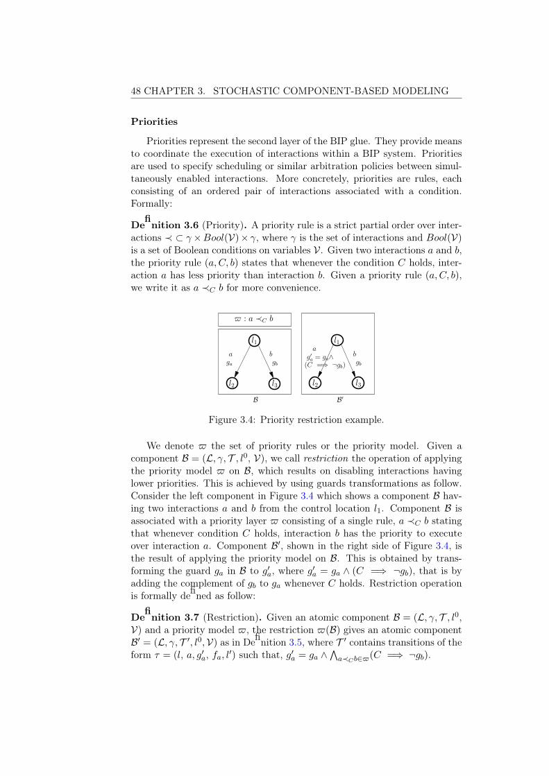
48 CHAPTER 3. STOCHASTIC COMPONENT-BASED MODELING
Priorities
Priorities represent the second layer of the BIP glue. They provide meansto coordinate the execution of interactions within a BIP system. Prioritiesare used to specify scheduling or similar arbitration policies between simul-taneously enabled interactions. More concretely, priorities are rules, eachconsisting of an ordered pair of interactions associated with a condition.Formally:
Definition 3.6 (Priority). A priority rule is a strict partial order over inter-actions ≺ ⊂ γ×Bool(V)× γ, where γ is the set of interactions and Bool(V)is a set of Boolean conditions on variables V . Given two interactions a and b,the priority rule (a, C, b) states that whenever the condition C holds, inter-action a has less priority than interaction b. Given a priority rule (a, C, b),we write it as a ≺C b for more convenience.
gb
bga gb
ba
� : a ≺C b
l3
l1l1
l2 l3l2
B B�
(C =⇒ ¬gb)
ag�a = ga∧
Figure 3.4: Priority restriction example.
We denote � the set of priority rules or the priority model. Given acomponent B = (L, γ, T , l0, V), we call restriction the operation of applyingthe priority model � on B, which results on disabling interactions havinglower priorities. This is achieved by using guards transformations as follow.Consider the left component in Figure 3.4 which shows a component B hav-ing two interactions a and b from the control location l1. Component B isassociated with a priority layer � consisting of a single rule, a ≺C b statingthat whenever condition C holds, interaction b has the priority to executeover interaction a. Component B�, shown in the right side of Figure 3.4, isthe result of applying the priority model on B. This is obtained by trans-forming the guard ga in B to g�a, where g�a = ga ∧ (C =⇒ ¬gb), that is byadding the complement of gb to ga whenever C holds. Restriction operationis formally defined as follow:
Definition 3.7 (Restriction). Given an atomic component B = (L, γ, T , l0,V) and a priority model �, the restriction �(B) gives an atomic componentB� = (L, γ, T �, l0,V) as in Definition 3.5, where T � contains transitions of theform τ = (l, a, g�a, fa, l
�) such that, g�a = ga ∧�
a≺Cb∈�(C =⇒ ¬gb).

CHAPTER 3. STOCHASTIC COMPONENT-BASED MODELING 49
Example 3.4 (Following Example 3.3). In Example 3.3, the goal is to havea model acting as follow. Whenever the Sender writes data to the Buffer, theReceiver reads it before it gets overridden by a new data, since the Buffer hasa single memory location. That is, we should never have successive writesnor reads. The expected behavior is shown in Figure 3.5a.
In the model presented in Figure 3.3, this is performed using time syn-chronization. The Sender is forced to write data after 10 time units whilethe Receiver reads it after 5 time units. In this way they are expected toalternate production and consumption. As previously mentioned, the modelin Figure 3.3 exhibits non-determinism which actually alters the desired be-havior. Consider a situation where the Sender is writing data to the Bufferthrough the io1 connector. Meanwhile, the Receiver is waiting in locationl4. When t ≥ 5, both tick3 and in3 become enabled. A non-deterministicchoice is then performed among them. What may happen is that tick3 istaken 10 consecutive times, which implies that tick1 has also been taken 10times (ticks are strongly synchronized using toc connector). This enablesthe Sender to write new data to the Buffer while the previous one is not yetconsumed by the Receiver as shown in Figure 3.5b.
time
toc toc
Sender.out Receiver.in Sender.out
0 5 10. . .
(a) Expected behavior of the System
model
time
toc
Sender.out Sender.out Receiver.in
0 5 10. . .
(b) System actual behavior
Figure 3.5: Behavior of the System component in Figure 3.3.
To resolve such a situation, one may change the Buffer model in sucha way it does not allow successive reads nor writes which is very restrictivesince it does not allow components reuse. Another alternative consists touse priorities to force in and out actions, when enabled, to execute over tick.A priority model consists thus on
� : toc ≺C io1, toc ≺C io2
. The C condition in this case is simply true. The priority model � stipulatesthat whenever the participating ports in io1 or io2 are enabled simultane-ously with a tick, they will have the priority to execute. For instance, when
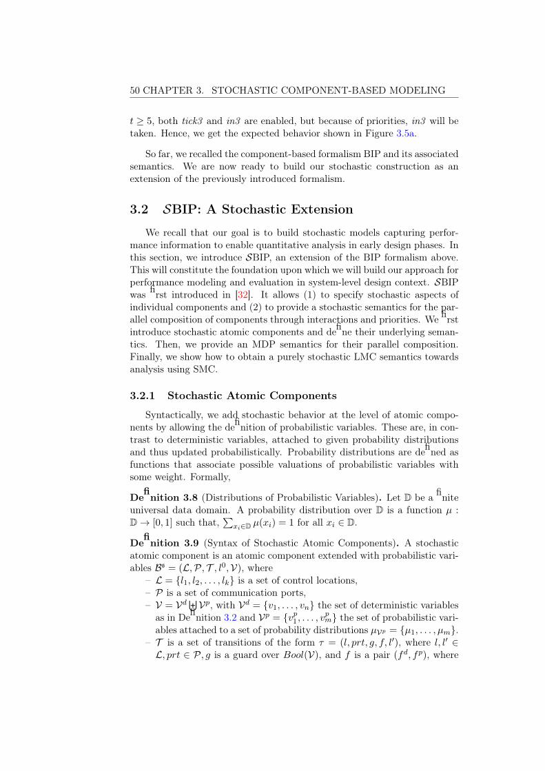
50 CHAPTER 3. STOCHASTIC COMPONENT-BASED MODELING
t ≥ 5, both tick3 and in3 are enabled, but because of priorities, in3 will betaken. Hence, we get the expected behavior shown in Figure 3.5a.
So far, we recalled the component-based formalism BIP and its associatedsemantics. We are now ready to build our stochastic construction as anextension of the previously introduced formalism.
3.2 SBIP: A Stochastic Extension
We recall that our goal is to build stochastic models capturing perfor-mance information to enable quantitative analysis in early design phases. Inthis section, we introduce SBIP, an extension of the BIP formalism above.This will constitute the foundation upon which we will build our approach forperformance modeling and evaluation in system-level design context. SBIPwas first introduced in [32]. It allows (1) to specify stochastic aspects ofindividual components and (2) to provide a stochastic semantics for the par-allel composition of components through interactions and priorities. We firstintroduce stochastic atomic components and define their underlying seman-tics. Then, we provide an MDP semantics for their parallel composition.Finally, we show how to obtain a purely stochastic LMC semantics towardsanalysis using SMC.
3.2.1 Stochastic Atomic Components
Syntactically, we add stochastic behavior at the level of atomic compo-nents by allowing the definition of probabilistic variables. These are, in con-trast to deterministic variables, attached to given probability distributionsand thus updated probabilistically. Probability distributions are defined asfunctions that associate possible valuations of probabilistic variables withsome weight. Formally,
Definition 3.8 (Distributions of Probabilistic Variables). Let D be a finiteuniversal data domain. A probability distribution over D is a function µ :D → [0, 1] such that,
�xi∈D µ(xi) = 1 for all xi ∈ D.
Definition 3.9 (Syntax of Stochastic Atomic Components). A stochasticatomic component is an atomic component extended with probabilistic vari-ables Bs = (L,P, T , l0,V), where
– L = {l1, l2, . . . , lk} is a set of control locations,– P is a set of communication ports,– V = Vd
�Vp, with Vd = {v1, . . . , vn} the set of deterministic variablesas in Definition 3.2 and Vp = {vp1 , . . . , vpm} the set of probabilistic vari-ables attached to a set of probability distributions µVp = {µ1, . . . , µm}.
– T is a set of transitions of the form τ = (l, prt, g, f, l�), where l, l� ∈L, prt ∈ P, g is a guard over Bool(V), and f is a pair (fd, fp), where

CHAPTER 3. STOCHASTIC COMPONENT-BASED MODELING 51
fd is a deterministic update function on V as in Definition 3.2, andfp ⊆ Vp is the subset of probabilistic variables to be updated on τ ,
– l0 is the initial location.
We define valuations of probabilistic variables as in the deterministiccase. We denote the set of valuations of a set of probabilistic variablesVp as DVp
. Vp is initially associated with a default valuation Xp0 ∈ DVp
.Each probabilistic variable vp ∈ Vp is attached to a probability distributionµ ∈ µVp , denoted as vp ∼ µ. Note that the used probability distributions arediscrete and assumed to be independent. We use small scripts xv
pto denote
valuations of single probabilistic variables vp ∈ Vp.
Semantics of Stochastic Atomic Components
The introduction of probabilistic variables at the level of atomic compo-nents engenders a probabilistic behavior over transitions. Let us considerthe atomic component Bs in Figure 3.6a. We graphically represent updateof probabilistic variables using � near variables names. Component Bs has aunique transition going from location l1 to location l2 using port prt whichupdates the probabilistic variable vp, defined over domain Dvp ⊆ D, accord-ing to the distribution µ : Dvp → [0, 1]. Assuming the initial value of vp
is xvp
0 , when executing Bs, there will be several possible transitions, havingthe same label prt, from state (l1, x
vp0 ) to states (l2, x
vpi ) for all xv
p
i ∈ Dvp asillustrated in Figure 3.6b. According to the definition of probabilistic vari-
l1
prt
vp = xp0
vp ∼ µ
vp�
l2
(a) A Stochastic Atomic Component Bs
(l1, xvp
0 )
µ
(l2, xvp
i )
prt prt
(b) Behavior of Bs
Figure 3.6: Example of a stochastic atomic component Bs and its behavior.
ables, the probabilities of these transitions will then be given by µ. Notethat when several probabilistic variables are updated, the resulting distribu-tion on transitions will be the product of the distributions associated to eachvariable as will be shown in Example 3.5. We recall that these distributionsare fixed during variables declaration, and are considered to be independentas stated in the beginning of this section.
Adapting the semantics of an atomic component in BIP as presented inDefinition 3.3 to atomic components with probabilistic variables leads to be-

52 CHAPTER 3. STOCHASTIC COMPONENT-BASED MODELING
haviors that combine both stochastic and non-deterministic aspects. Indeed,even if transitions are either purely deterministic or purely stochastic 3, sev-eral transitions can be enabled in a given state. In such a case, the choicebetween them is non-deterministic as explained in the BIP background sec-tion.
Consider a stochastic component Bs = (L,P, T , l0,V). Given a state
(l;Xp;X) in L×DVp×DVd, we denote by Enabled(l;Xp;X) the set of transi-
tions in T that are enabled in that state, i.e. transitions τ = (l, prt, g, f, l�) ∈T , such that g(Xp;X) is satisfied. Remark that the set Enabled(l;Xp;X)may have a cardinality |Enabled(l;Xp;X)| ≥ 1, as explained earlier. Inthe associated semantics of Bs, a non-deterministic choice between portsin Enabled(l;Xp;X) is first performed. Then, probabilistic selection of thenext state is done according to distributions attached to probabilistic vari-ables updated on the transition labeled by the selected port. The semanticsof a stochastic atomic component is thus an MDP as formally stated below:
Definition 3.10. The semantics of a stochastic atomic component Bs =(L,P, T , l0,V) is a Markov Decision Process M = �S,Act, ι,π,Σ, L�, where
– S = L × DVp × DVdis the set of states,
– Act = P is the set of actions,– ι(l0) = 1 is the initial probability distribution,– Σ is the set of atomic proposition over V ,– L : S → Σ is the state labeling function,
– π : S ×Act× S → [0, 1] contains transition of the form sprt−→ s� where
s = (l;Xp;X) and s� = (l�;X �p;X �) for some τ = (l, prt, g, (fd, fp), l�) ∈Enabled(l;Xp;X) where,
X �p(vp) = Xp(vp) for all vp /∈ fp
X �p(vp) = xvp
for each vp ∈ fp, where xvp ∈ Dvp ,
(X ��p, X �) = fd(X �p, X), and the probability to take a transition isdefined using µVp , the set of probability distributions attached to Vp
as follow:
π(s, prt, s�) =�
vp∈fp
µvp(xvp)
Let Bs be a stochastic atomic component and M be the associatedMDP. A state s ∈ S is seen as the combination of a control location l ∈ Lwith the valuations of the probabilistic and deterministic variables, respec-tively Xp and X. We write s = (l;Xp;X). The set of enabled actionsin some state Act(s) corresponds to the set of ports labeling transitionsτ ∈ Enabled(l;Xp;X), where s = (l;Xp;X). That is, Act(s) = {prt ∈P | τ = (l, prt, g, (fd, fp), l�) ∈ Enabled(l;Xp;X)}.
3. In the sense that they are associated or not with probabilistic variables.

CHAPTER 3. STOCHASTIC COMPONENT-BASED MODELING 53
From now on, we will use Act(s) to denote the set of ports enabled insome state s of a stochastic atomic component and ports labels to denotetransitions. We will also adopt the prt-successor notation from the MDPdefinition in Chapter 2.
In each state s ∈ S, we select a port prt ∈ Act(s) non-deterministically.We recall that all variables vp ∈ Vp are defined over domains Dvp ⊆ DVp
and are associated with distributions vp ∼ µvp . A prt-successor state s� =(l;X �p;X �) is obtained by:
1. Keeping valuations of non-updated probabilistic variables on prt un-changed, i.e., ∀vp /∈ fp, X �p(vp) = Xp(vp),
2. Assigning new valuations xvp ∈ Dvp to updated ones, i.e., ∀vp ∈
fp, X �p(vp) = xvp, and
3. Updating variables according to fd, i.e., (X ��p, X �) = fd(X �p, X).
The probability of a transition sprt−→ s� is the product of the distributions
µvp of all vp ∈ fp, that is�
vp∈fp µvp(xvp).
Example 3.5. Consider a stochastic atomic component Bs having three lo-cations l1, l2, and l3 and two enabled transitions prt1 and prt2 from l1 to l2and l3 respectively, as shown in Figure 3.7a. Transition prt1 is associatedwith a probabilistic variable vp1 ∼ µ1 and prt2 is associated with two proba-bilistic variables vp2 ∼ µ2 and vp3 ∼ µ3. Moreover, vp1 is defined over domainD1 = {1, 2}, and vp2 and vp3 are respectively defined over domains D2 = {3, 4}and D3 = {true, false}. The probabilities of variables valuations are givenby the associated distributions.
In the underlying MDP semantics depicted in Figure 3.7c, we find theenabled actions prt1 and prt2, each unfolded with respect to its associatedprobability distribution as defined in the Bs component. For instance, weidentify two transitions labeled prt1 having probabilities µ1(1) and µ1(2). Forprt2, since its is associated with two probabilistic variables in Bs, we obtainfour transitions labeled prt2, due to the product µ2µ3, having the probabil-ities µ2(3)µ3(true), µ2(3)µ3(false), µ2(4)µ3(true), and µ2(4)µ3(false).
Example 3.6 (Part of a Stochastic Multimedia Stream Source). In thisexample, we model the stochastic behavior of an MPEG2-coded video streamsource. This will actually be part of the input stream model for the videodecoding system initially introduced in Example 3.2. In this sub-model of theinput stream source, we only consider frames generation. An MPEG2-codedstream is composed of coded video frames of three types, namely I,P, and B[133]. These are organized following a predefined Group Of Pictures (GOP)pattern: IBBPBBPBBPBB, IBBPBBPBBPBB, . . . Figure 3.8 showsan SBIP component modeling this behavior, where frames sizes are producedin a probabilistic fashion following three different probability distributions(µi, µp, µb), each corresponding to a frame type.

54 CHAPTER 3. STOCHASTIC COMPONENT-BASED MODELING
prt1 prt2vp2�vp1�
l1
l3
vp3�
vp2 ∼ µ3
l2
vp1 ∼ µ1vp1 = 1vp2 = 3 vp2 ∼ µ2
vp3 = false
(a) A Stochastic BIP Component Bs
(l1; 1, 3, false)
(l3; 1, 4, false)(l3; 1, 4, true)
prt1 prt2
µ2µ3
(l3; 1, 3, false)
µ1
(l3; 1, 3, true)
(l2; 2, 3, false)(l2; 1, 3, false)
(b) Underlying Behavior of Bs
s1
s2
s3
s4
s5
s6
s7
prt2, µ2(4)µ3(false)
prt1, µ1(1)
prt1, µ1(2)
prt2, µ2(3)µ3(true)
prt2, µ2(4)µ3(true)
prt2, µ2(3)µ3(false)
(c) The MDP semantics of Bs
Figure 3.7: Example of a stochastic atomic component Bs and its underlyingsemantics when several transitions are simultaneously enabled.
generate
generate
generate
generate
generate
l1
l3
l4
l2
vpb�
vpb�
x = x+ 1
vpi �
vpi ∼ µivpp ∼ µp
x = 0
fs = vpi
[x ∈ {3, 6, 9}]
fs = vpbx = x+ 1
fs = vpb
vpb�
[x == 12]
fs = vpp
vpi �vpb ∼ µb
x = x+ 1
x = 0fs = vpi
vpp�x = x+ 1fs = vpb
Figure 3.8: Stochastic Multimedia Stream Source model: frames generatorcomponent.
Till now, we saw that the semantics of an SBIP component is defined asa Markov Decision Process. In the next section we provide definitions forassembling stochastic components using BIP composition operators.

CHAPTER 3. STOCHASTIC COMPONENT-BASED MODELING 55
3.2.2 Composition of Stochastic Components
In this section we define the semantics of the parallel composition ofstochastic atomic components. In this context, compositional operators areunchanged, that is, we adopt the same definitions of interactions (Defini-tion 3.4) and priorities (Definition 3.6). For the sake of simplicity, we restrictdata transfer functions on interactions to be deterministic. Thus, probabilis-tic and deterministic variables are transferred in a deterministic way.
When considering a system with n stochastic components Bsi = (Li,Pi, Ti,
l0i ,Vi) and a set of interactions γ, the construction of the product componentBs = γ(Bs
1, . . . ,Bsn) is performed as in BIP. Formally:
Definition 3.11. (Composition of Stochastic Components) Given a set ofinteractions γ, the composition of n stochastic components γ(Bs
1, . . . ,Bsn),
where Bsi = (Li,Pi, Ti, l0i ,Vi) is a stochastic atomic component Bs = (L,γ, T ,
l0,V) where,
– L = L1 × . . .× Ln, is a set of control locations,– γ is the set of ports,– T contains transitions of the form τ = ((l1, . . . , ln), a,Ga, (F
da , F
pa ),
(l�1, . . . , l�n)) obtained by synchronization of sets of transitions {τi =
(li, prti, gi, fi, l�i) ∈ Ti}i∈I such that,
– a = {prti}i∈I ∈ γ,– Ga = ga ∧
�i∈I gi,
– F da = fd
a ��i∈I f
di ,
– F pa =
�i∈I f
pi , and
– l�j = lj if j /∈ I,
– l0 = l01 × . . .× l0n,– V =
�ni=1 Vi, is the set of deterministic and probabilistic variables.
Restriction operation over stochastic atomic components is performedusing priority rules in Definition 3.6. It consists of the same guards trans-formation operation presented in Definition 3.7. Thus, it produces a newstochastic component.
By construction, as assembling stochastic atomic components using com-position operators (composition and restriction) produces a stochastic atomiccomponent, its semantics is a Markov Decision Process given by Defini-tion 3.10.
Example 3.7. Consider the stochastic BIP components Bs1 and Bs
2 given inFigure 3.9a. Bs
1 has a single probabilistic variable vp1 , defined over domainD1 and attached to distribution µ1, and a single transition from locationl11 to location l12 using port prt1, where vp1 is updated. In location l11, thevariable vp1 is assumed to have value xp0 ∈ D1. Bs
2 has two probabilisticvariables vp2 and vp3 respectively defined over domains D2 and D3, to whichare attached distributions µ2 and µ3 respectively. Bs
2 has two transitions: a
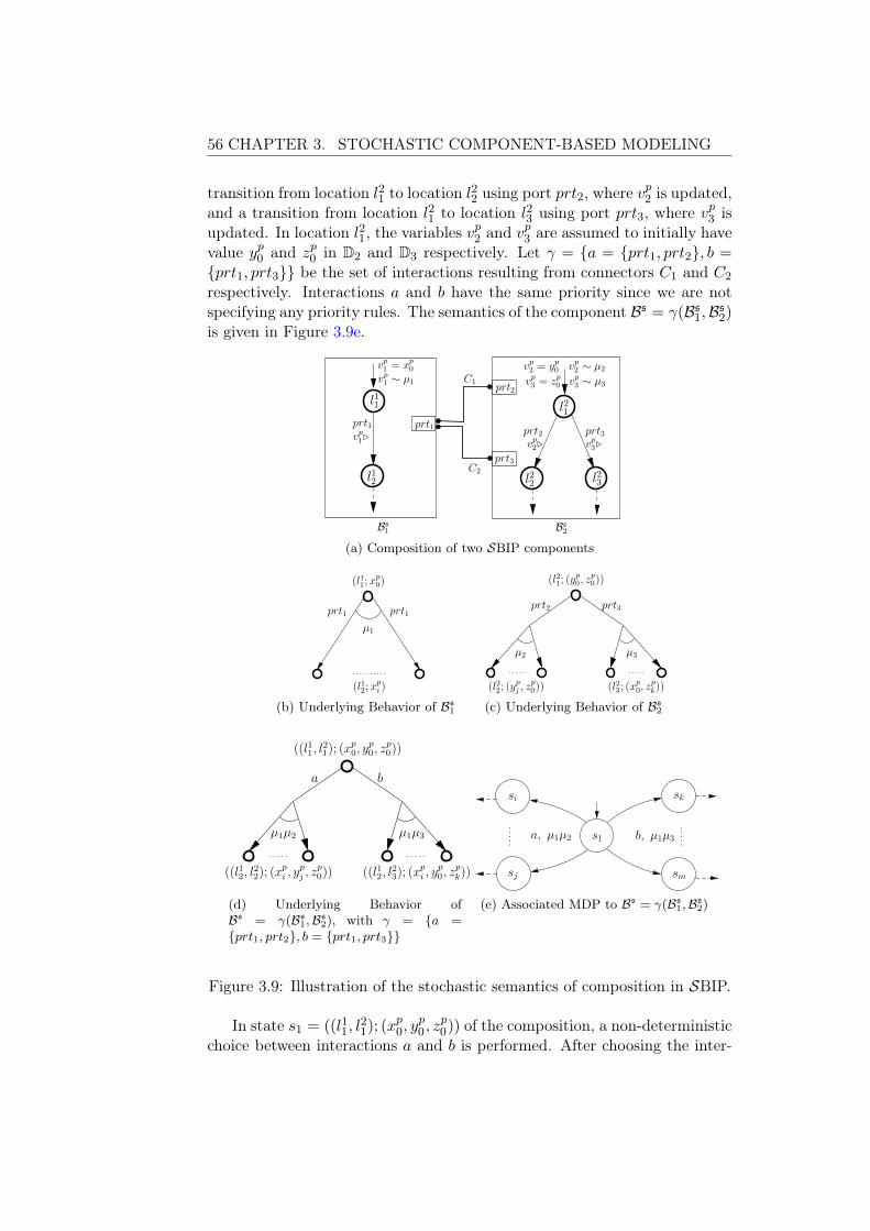
56 CHAPTER 3. STOCHASTIC COMPONENT-BASED MODELING
transition from location l21 to location l22 using port prt2, where vp2 is updated,and a transition from location l21 to location l23 using port prt3, where vp3 isupdated. In location l21, the variables vp2 and vp3 are assumed to initially havevalue yp0 and zp0 in D2 and D3 respectively. Let γ = {a = {prt1, prt2}, b ={prt1, prt3}} be the set of interactions resulting from connectors C1 and C2
respectively. Interactions a and b have the same priority since we are notspecifying any priority rules. The semantics of the component Bs = γ(Bs
1,Bs2)
is given in Figure 3.9e.
prt2 prt3vp3�vp2�
l22
l21
vp3 = zp0
prt1prt1
vp1 ∼ µ1
l12
l11
vp2 = yp0vp1 = xp0
vp1�
prt3
vp2 ∼ µ2
vp3 ∼ µ3
l23
prt2
Bs2Bs
1
C2
C1
(a) Composition of two SBIP components
(l11; xp0)
µ1
prt1 prt1
(l12; xpi )
(b) Underlying Behavior of Bs1
(l22; (ypj , z
p0))
(l21; (yp0, z
p0))
µ2 µ3
prt2 prt3
(l23; (xp0, z
pk))
(c) Underlying Behavior of Bs2
((l12, l22); (x
pi , y
pj , z
p0))
((l11, l21); (x
p0, y
p0, z
p0))
µ1µ2 µ1µ3
a b
((l12, l23); (x
pi , y
p0, z
pk))
(d) Underlying Behavior ofBs = γ(Bs
1,Bs2), with γ = {a =
{prt1, prt2}, b = {prt1, prt3}}
s1
si
sj
b, µ1µ3
sk
sm
a, µ1µ2
(e) Associated MDP to Bs = γ(Bs1,Bs
2)
Figure 3.9: Illustration of the stochastic semantics of composition in SBIP.
In state s1 = ((l11, l21); (x
p0, y
p0 , z
p0)) of the composition, a non-deterministic
choice between interactions a and b is performed. After choosing the inter-

CHAPTER 3. STOCHASTIC COMPONENT-BASED MODELING 57
action, the corresponding transition is taken, updating the correspondingprobabilistic variables with the associated distributions. As an example, theprobability of going to state ((l12, l
22); (x
pi , y
pj , z
p0)), where xpi ∈ D1 and ypj ∈ D2,
after non-deterministically choosing interaction a is µ1(xpi )µ2(y
pj ), while the
probability of going to state ((l12, l23); (x
pi , y
p0 , z
pk)), x
pi ∈ D1 and zpk ∈ D3, after
non-deterministically choosing interaction b is µ1(xpi )µ3(z
pk).
Example 3.8 (Stochastic Multimedia Stream Source). This example depictsthe full stochastic multimedia stream source model started in Example 3.6.The underlying model is a composition of three components consisting ofthe Frames Generator (see Example 3.6), a Splitter, and a Transfer Mediacomponent. The generated output stream is made of macro-blocks whichare going to be stored in the input buffer of the decoding unit. The numberof bits (the size) of every macro-block, together with a bit-rate parameterof the transfer media, determine the arrival time of the macro-block to thebuffer. This number of bits is specific for each macro-block type (w.r.t frametypes) and follows a specific probability distribution (µmb) parametrized byframe sizes.
Figure 3.10 shows the SBIP component modeling this behavior. Framesare produced following the GOP pattern as explained earlier in Example 3.6.Each frame is split into 330 micro-blocks, having probabilistically distributedsizes, by the Splitter component. Each macro-block is then sent for storagethrough the Transfer Media component which model the arrival time ofmacro-blocks to the buffer.
The components are assembled together using two connectors C1 andC2 providing data transfer facilities. The first connector enables deliveringframes to the Splitter, whereas the second ensures the transfer of the gener-ated macro-blocks to the Transfer Media component. Finally, it is worth tomention that the transfer and tick ports of the Transfer Media componentare made available as interfaces for the Source component to communicatewith the rest of the video decoding system model presented later in thechapter.
Stochastic atomic components as well as their composition have an MDPsemantics that encompasses non-deterministic and probabilistic decisions.However, to be able to perform quantitative analysis such as SMC on thesemodels, it is required to resolve any non-determinism. In the following, weshow how to reduce SBIP models to produce a purely stochastic semantics.
3.2.3 Purely Stochastic Semantics
Building rich stochastic performance models and using SMC to quanti-tatively analyze them is the main motivation behind the proposed stochasticextension. To this end, one needs to produce a purely stochastic behaviorwhere only probabilistic choices are possible. Given the SBIP construction

58 CHAPTER 3. STOCHASTIC COMPONENT-BASED MODELING
generate
generate
generate
generate
generate
get_mb
transferresume
generate_mb
get_frame
get_frame get_mb transfer
tick
split
generate_mbgenerate
C1 C2
tick
transfer
Splitter Transfer MediaFrames Generator
tick
l1
l3
l4
l2
vpb�
x = x+ 1
vpi �
vpi ∼ µivpp ∼ µp
x = 0
[x ∈ {3, 6, 9}]
f = vpbx = x+ 1
f = vpb
vpb�
[x == 12]
f = vpp
vpb ∼ µb
x = x+ 1
x = 0f = vpi
vpp�
l1l1
l2
l3 l2
[period == 0]
period = mb.size/bit_rate
y = y + 1
[y == 330]
y = 0
y = 0
[y < 330]
vpmb�
x = x+ 1f = vpb
vpb�
f = vpivpi �
tmp period = 0tmpf mb mb
period
vpmb ∼ µmb(tmp) vpmb
period = period− 1t = t+ 1
tmp = f mb = vpmb
Figure 3.10: SBIP component of an MPEG2 Stream Source.
above, we propose to use probabilistic schedulers in order to produce a purelystochastic LMC semantics of SBIP models. We first define the semantics ofa purely stochastic component. Then, adapt the definition of schedulers inChapter 2 and provide definition of the induced LMC in this context.
In chapter 2, we introduced schedulers and shown that it yields MarkovChain semantics, when applied on MDPs. We build upon chapter 2 defini-tions to define schedulers for SBIP models. We recall that non-determinismoccurs in SBIP models, whenever several interactions are simultaneouslyenabled. A scheduler, in this context, provides probability distributions toselect among enabled interactions in global states as in Definition 2.8. Givena stochastic atomic component and a scheduler S , the produced behavioris purely stochastic. It allows probabilistic choices between transitions inAct(s) instead of non-deterministic choices. The resulting underlying be-havior is thus a Markov Chain as given by Definition 2.9.
Let Bs = (L,P, T , l0,V) be a stochastic atomic component and M =�S,Act, ι,π,Σ, L� the associated MDP semantics. In the Markov ChainMS = �S, ι,π�,Σ, L� induced by the scheduler S on Bs, the probability
of taking transition s −→ s� ∈ π� corresponding to transition sprt−→ s� ∈ π,
where s = (l;Xp;X) and s� = (l;X �p;X �) ∈ S and τ = (l, prt, g, (fd, fp), l�) ∈Act(s) is computed as follows. A probabilistic choice over enabled transitionsin Act(s) using the distribution provided by S is performed first, followed bya probabilistic choice using probability distributions attached to probabilisticvariables as earlier, that is,
π�(s, s�) =�
sprt−→s�
(S (s, prt) ·�
vp∈fp
µvp(xvp))
Example 3.9 (Induced Markov Chain by a Uniform Scheduler on the MDPFigure 3.7c). Consider the SBIP model and its associated MDP in Exam-ple 3.5 where non-determinism appears only on state s1 = (l1; 1, 3, false),

CHAPTER 3. STOCHASTIC COMPONENT-BASED MODELING 59
where Act(s1) = {prt1, prt2}. In order to resolve this non-determinism andproduce a fully stochastic behavior, we may use a scheduler S that uniformlyselects among enabled actions in each state. Hence, ∀s ∈ S, each prt ∈Act(s) has an equal probability to be selected. In this case,
S (s1, prti) =1
|Enabled(s1)|=
1
2, where 1 ≤ i ≤ 2.
Figure 3.11 depicts the induced Markov Chain. In this example, the differ-ence between the MDP and the induced LMC is at the level of probabili-ties of transitions (no structural transformation has been operated). Theseare obtained by multiplying the probabilities of the MDP transition by thescheduler value, that is, 1
2 .
s1
s2
s3
s4
s5
s6
s7
12µ2(3)µ3(false)
12µ2(4)µ3(false)
12µ2(3)µ3(true)1
2µ1(1)
12µ1(2)
12µ2(4)µ3(true)
Figure 3.11: LMC induced by a uniform scheduler S on the MDP Fig-ure 3.7c.
It is worth mentioning that defining probabilistic schedulers for SBIPmodels that encompass non-deterministic behavior requires a bit of care. Letus consider a component Bs and its associated MDP semantics M. Given astate s ∈ S, where three actions are possible {�, ς,ϑ}, it is not sufficient to de-fine a single probability distribution over them, but we need to specify a prob-ability distribution for each possible Act(s). Actually, the non-determinismimplies that we don’t have any apriori knowledge about which actions will beenabled each time, that is, Act(s) ∈ {{�, ς,ϑ}, {�, ς}, {�,ϑ}, {ς,ϑ}, {�}, {ς}},or {ϑ}. This is tedious to do for each state of the model especially in forindustrial-size models. In the current state of this work, we stick to uni-form distributions which implicitly takes into account the number of en-abled actions in Act(s), i.e. ∀� ∈ Act(s),π(s, �, s�) = 1
|Act(s)| . Details oninvestigating possible representation of probabilistic schedulers with othersprobability distributions in SBIP are discussed as perspective work in theconclusion chapter of the manuscript.
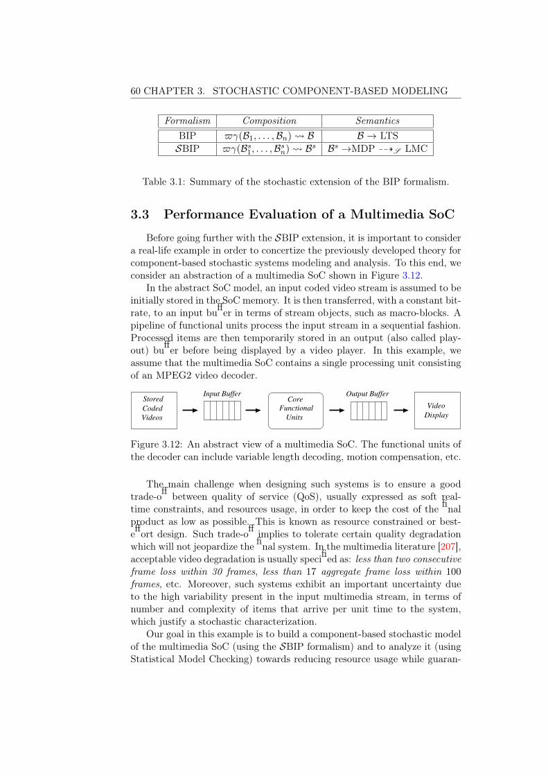
60 CHAPTER 3. STOCHASTIC COMPONENT-BASED MODELING
Formalism Composition Semantics
BIP �γ(B1, . . . ,Bn) � B B → LTS
SBIP �γ(Bs1, . . . ,Bs
n) � Bs Bs →MDP ���S LMC
Table 3.1: Summary of the stochastic extension of the BIP formalism.
3.3 Performance Evaluation of a Multimedia SoC
Before going further with the SBIP extension, it is important to considera real-life example in order to concertize the previously developed theory forcomponent-based stochastic systems modeling and analysis. To this end, weconsider an abstraction of a multimedia SoC shown in Figure 3.12.
In the abstract SoC model, an input coded video stream is assumed to beinitially stored in the SoC memory. It is then transferred, with a constant bit-rate, to an input buffer in terms of stream objects, such as macro-blocks. Apipeline of functional units process the input stream in a sequential fashion.Processed items are then temporarily stored in an output (also called play-out) buffer before being displayed by a video player. In this example, weassume that the multimedia SoC contains a single processing unit consistingof an MPEG2 video decoder.
Core
Functional
Units
Stored
Coded
Videos Display
Video
Output BufferInput Buffer
Figure 3.12: An abstract view of a multimedia SoC. The functional units ofthe decoder can include variable length decoding, motion compensation, etc.
The main challenge when designing such systems is to ensure a goodtrade-off between quality of service (QoS), usually expressed as soft real-time constraints, and resources usage, in order to keep the cost of the finalproduct as low as possible. This is known as resource constrained or best-effort design. Such trade-off implies to tolerate certain quality degradationwhich will not jeopardize the final system. In the multimedia literature [207],acceptable video degradation is usually specified as: less than two consecutiveframe loss within 30 frames, less than 17 aggregate frame loss within 100frames, etc. Moreover, such systems exhibit an important uncertainty dueto the high variability present in the input multimedia stream, in terms ofnumber and complexity of items that arrive per unit time to the system,which justify a stochastic characterization.
Our goal in this example is to build a component-based stochastic modelof the multimedia SoC (using the SBIP formalism) and to analyze it (usingStatistical Model Checking) towards reducing resource usage while guaran-

CHAPTER 3. STOCHASTIC COMPONENT-BASED MODELING 61
tying a tolerable loss in video quality. We will mainly focus on the firstspecification of tolerable video degradation, i.e., less than two consecutiveframe loss within 30 frames, while trying to reduce the buffer sizes. A Frameloss is seen at the player end. The latter starts reading decoded items afteran initial delay (also called play-out delay). Reads are then performed peri-odically from the output buffer. A loss happens when the player do not findthe required items to display in a specific period. This is denoted as bufferunderflow and can be interpreted as a deadline miss, that is, the decodingunit failed to provide the required items in time. Figure 3.13 illustrates suchbehavior.
0 2 4 6 8 10 12 14 16
x 109
0
100
200
300
400
500
600
700
800
Time (ns)
Num
ber
of m
acro
-blo
cks
Play-out Buffer Fill-levelPlay-out Buffer Underflow
Figure 3.13: Evolution of the play-out buffer fill-level over time. It alsoshows the buffer underflow evolution. This is obtained by simulating theSBIP model below with an initial delay equal to 75 ms.
Our goal is to estimate the probability that buffer underflow (denotedU) is less than two consecutive frames in 30 frames, given the followingparameters of the multimedia SoC:
– A set of video clips of certain bit-rate (r) and resolution,– The maximum frequency of the MPEG2 decoding unit (f),– The consumption rate of the player device (c),– The start-up values for the initial delay (d), input buffer size (ibs), and
play-out buffer size (obs).
3.3.1 SBIP Model of the Multimedia SoC
The SBIP model of the multimedia SoC is obtained in a straightforwardmanner from the description above. It has a component for each part ofthe SoC shown in Figure 3.12. This model captures the stochastic behaviorof the system in the following way. The coded object’s arrival time to theinput buffer follows defined probability distributions which are constructedfrom a given set of video clips (See Figure 3.14). Thus, the decoded object’sarrival to the output buffer is also probabilistic, which leads to probabilistic
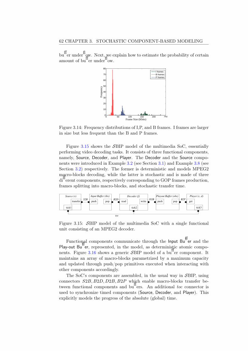
62 CHAPTER 3. STOCHASTIC COMPONENT-BASED MODELING
buffer underflow. Next, we explain how to estimate the probability of certainamount of buffer underflow.
0 50 100 150 200 2500
10
20
30
40
50
60
70
80
Frame Size (Kbits)
Fre
quen
cy
I framesB framesP frames
Figure 3.14: Frequency distributions of I,P, and B frames. I frames are largerin size but less frequent than the B and P frames.
Figure 3.15 shows the SBIP model of the multimedia SoC, essentiallyperforming video decoding tasks. It consists of three functional components,namely, Source, Decoder, and Player. The Decoder and the Source compo-nents were introduced in Example 3.2 (see Section 3.1) and Example 3.8 (seeSection 3.2) respectively. The former is deterministic and models MPEG2macro-blocks decoding, while the latter is stochastic and is made of threedifferent components, respectively corresponding to GOP frames production,frames splitting into macro-blocks, and stochastic transfer time.
pop
Source (r) Decoder (f) Player (c, d)
tick1 tick2 tick3
read write push
Input Buffer (ibs)
push pop
Playout Buffer (obs)
transfer get
toc
S2B B2D D2B B2P
Figure 3.15: SBIP model of the multimedia SoC with a single functionalunit consisting of an MPEG2 decoder.
Functional components communicate through the Input Buffer and thePlay-out Buffer, represented, in the model, as deterministic atomic compo-nents. Figure 3.16 shows a generic SBIP model of a buffer component. Itmaintains an array of macro-blocks parametrized by a maximum capacityand updated through push/pop primitives executed when interacting withother components accordingly.
The SoC’s components are assembled, in the usual way in SBIP, usingconnectors S2B,B2D,D2B,B2P which enable macro-blocks transfer be-tween functional components and buffers. An additional toc connector isused to synchronize timed components (Source, Decoder, and Player). Thisexplicitly models the progress of the absolute (global) time.
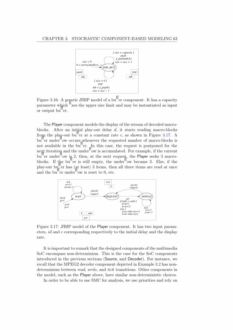
CHAPTER 3. STOCHASTIC COMPONENT-BASED MODELING 63
[ size < capacity ]push
f_push(mb,b)size = 0
b = (array)malloc(...)SND_RCV
mb
push
[ size > 0 ]pop
mb = f_pop(b)
size = size + 1
size = size − 1
mb
pop
Figure 3.16: A generic SBIP model of a buffer component. It has a capacityparameter which fixes the upper size limit and may be instantiated as inputor output buffer.
The Player component models the display of the stream of decoded macro-blocks. After an initial play-out delay d, it starts reading macro-blocksfrom the play-out buffer at a constant rate c, as shown in Figure 3.17. Abuffer underflow occurs whenever the requested number of macro-blocks isnot available in the buffer. In this case, the request is postponed for thenext iteration and the underflow is accumulated. For example, if the currentbuffer underflow is 2, then, at the next request, the Player seeks 3 macro-blocks. If the buffer is still empty, the underflow became 3. Else, if theplay-out buffer has (at least) 3 items, then all three items are read at onceand the buffer underflow is reset to 0, etc.
REQUEST DISPLAY
q=1id=d
request
[id=0]
WAIT
u=0
tickt=t+1p=p−1
request[p=0]
mbsq
tick
p
p=c
id=id−1t=t+1tick
getif (mbs = null) {
q=q+1u=u+1}
else {q=q−mbs.size+1u=u−mbs.size}
get
Figure 3.17: SBIP model of the Player component. It has two input param-eters, id and c corresponding respectively to the initial delay and the displayrate.
It is important to remark that the designed components of the multimediaSoC encompass non-determinism. This is the case for the SoC componentsintroduced in the previous sections (Source, and Decoder). For instance, werecall that the MPEG2 decoder component depicted in Example 3.2 has non-determinism between read, write, and tick transitions. Other components inthe model, such as the Player above, have similar non-deterministic choices.
In order to be able to use SMC for analysis, we use priorities and rely on

64 CHAPTER 3. STOCHASTIC COMPONENT-BASED MODELING
a uniform scheduler to resolve such non-deterministic behavior. For instancethe following priority model is used to enable components progress:
� : toc < S2B, toc < B2D, toc < D2B, toc < B2P.
This gives high priority to decode macro-blocks and to transfer them, whenenabled, over time progress.
3.3.2 QoS Requirements Evaluation
To evaluate QoS requirements of the multimedia SoC, we apply statisticalmodel checking on the SBIP model presented above. Before presenting theexperiment details, it is worth to report some important observations withrespect to the SoC model operation.
We previously stated that play-out buffer underflow is observed at thePlayer end, and that this component has two parameters c and d, respec-tively defining the initial delay after which it has to start reading from thebuffer, and the periodicity of reading. Both parameters, together with thedecoder frequency and the arrival time of macro-blocks to the input buffer,have an impact on buffer underflow. Actually, when the initial delay is high,and when both the decoder and the arrival time are not too slow, the play-out buffer will accumulate an important number of macro-blocks before theplayer starts reading 4, which reduces the probability of occurrence of un-derflow later on. In the opposite scenario, the probability of having bufferunderflow becomes higher.
In the following experiments, the decoder frequency, the macro-blocksarrival time to the input buffer 5, as well as the periodicity of the Playerare considered to be fixed. We will try to tune the remaining parameters,such that to obtain a good trade-off between the play-out buffer size and theprobability of having two consecutive frames loss within 30 frames.
In order to estimate the probability of this requirement, we use an Ob-
server which monitors the occurrence of the frames loss. This will run inparallel with the SoC components and reacts to relevant events related tothe property of interest, that is, play-out buffer pops. We exploit BIP ex-pressiveness to encode the observer behavior as an atomic component whichwill be connected to the B2P connector between the play-out buffer and thePlayer. As shown in Figure 3.18, the Observer has three states: OK, PAR-
TIAL, and FAIL. The FAIL state capture the fact that two consecutive frameswithin 30 have been lost. The component starts in the OK state. When asingle frame is lost, the observer moves from state OK to PARTIAL. Later,if there is an additional frame loss, within the same window of 30 frames,
4. A very high initial delay requires an big play-out buffer size and may induce a bufferoverflow. In this experiment, we are only focusing on buffers underflow.
5. This is defined by the bit-rate of the considered video clips.

CHAPTER 3. STOCHASTIC COMPONENT-BASED MODELING 65
[ lost = true ]lost1frame
observe
[ lost = true ]lost2frames
lost
success
if ( frames = 30 )frames = frame + 1
{ lost = false frames = 0 }
PARTIALOK FAIL
[ frames = 30 v lost = false ]
observeframes = frame + 1
lost = falseif ( frames = 30 ) frames = 0
frames = 0
lost = false
observe
Figure 3.18: SBIP model of the Observer component. It models the QoSproperty to be verified. The variable frame counts the number of frames tocheck if two consecutive loss occurs within a second (i.e. within 30 frames).The read port of the Observer is synchronized with the read port of thePlayer. A variable lost is associated with the read port records a frame loss.
the Observer moves to the FAIL state. Otherwise, when no additional losseshappen within that widow, it moves back to the OK state.
Analysis and Results
This section sketches QoS requirement probabilities estimated using thestatistical model checking technique. The experiments were conducted forlow bit-rates and low resolution clips (352 ∗ 240) obtained from an opensource 6. The bit-rate of the input videos is 1.5 Mbits per second and theframe output rate is 30 frames per seconds (fps). We used an MPEG2implementation optimized for speed 7. The MPEG2 source was annotatedto get the number of bits corresponding to each compressed macro-block.The execution cycles for each macro-block is obtained from the processorsimulator SimpleScalar 8. We chose the video files cact.m2v, mobile.m2v,
and tennis.m2v for our experiments.Recall that we used the observer component to monitor events corre-
sponding to two consecutive frames loss within 30 frames (which is equiva-lent to 1 second given the frame output rate of 30 fps). As explained earlier,this raises a flag denoted lost whenever it catches that event. Thus, we usedthe following BLTL property to query the SoC model with respect to theprobability to never get two consecutive frames loss within a second.
φ = Gt(¬lost)
We choose t = 1500000 steps, such that to display all the macro-blocks ofeach video clip. Note that all the considered clips are composed of 148500
6. ftp://ftp.tek.com/tv/test/streams/Element/index.html
7. http://libmpeg2.sourceforge.net
8. http://www.simplescalar.com/

66 CHAPTER 3. STOCHASTIC COMPONENT-BASED MODELING
macro-blocks, that is, 450 frames. Finally, we applied SMC with inputs theSoC model, the BLTL property φ and the confidence parameters δ = 5 10−2
and α = β = 10 −2. We did measure the probability of φ for different play-out delay values and observed the play-out buffer fill-level evolution. Werepeated the same experiment for the three video clips selected previously.
0,230.160.10.050380
400
420
440
460
480
500
520
540
560
580
1 - P()
Buf
fer
fill
-lev
el (
in K
Byt
es)
170 130 120
Play-out Delay (in milliseconds)140 135
Figure 3.19: Play-out buffer fill-level and probability of φ for various play-out delay values for cact.m2v. For this video clip, the processor frequencyis set to 109 Mhz.
Figures 3.19, 3.20, and 3.21 plots the results of the play-out buffer fill-levelfor various play-out delay values, and corresponding probabilistic bounds. Inthese figures, we report, in the X axis, the probability of eventually havingtwo consecutive frames loss withing a second, i.e., (1− P (φ)). The play-outbuffer fill-level and the play-out delay evolution are respectively depicted inthe Y and Z axis (in the top).
Let us first focus on the impact of the play-out delay on the probabilityof φ. As expected, one can see that increasing the play-out delay reducesthe probability of eventual underflow (1−P (φ)) for the different video clips.With respect to the buffer fill-level, we observe that it reduces substantiallyeven for a small decrease of probabilistic value. For instance, there could bea buffer size reduction of 40% for an increase in the value of the probabilisticbound from 0 to 0.2 (Figures 3.20). In fact the buffer savings can be largerif we compare the buffer size required for no underflow and the memoryrequired for the QoS property to be always true. It is worth mentioningthat these results confirm our claim that, for tolerable degradation in videoquality, output buffer size could be significantly reduced compared to thebuffer size required for playing lossless videos.
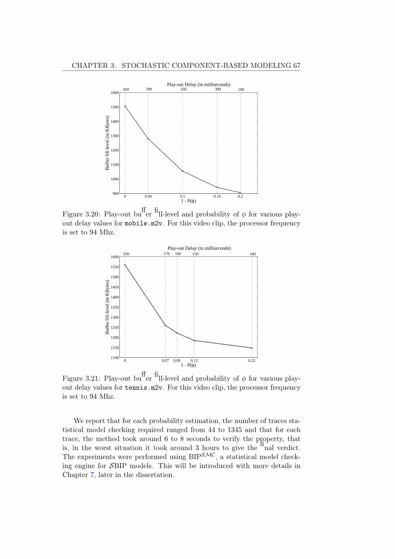
CHAPTER 3. STOCHASTIC COMPONENT-BASED MODELING 67
0,20.160.10.040900
1000
1100
1200
1300
1400
1500
1600
1 - P()
Buf
fer
fill
-lev
el (
in K
Byt
es)
450 390 330 300 290Play-out Delay (in milliseconds)
Figure 3.20: Play-out buffer fill-level and probability of φ for various play-out delay values for mobile.m2v. For this video clip, the processor frequencyis set to 94 Mhz.
0 0,07 0,09 0.12 0.221100
1150
1200
1250
1300
1350
1400
1450
1500
1550
1600
1 - P()
Buf
fer
fill
-lev
el (
in K
Byt
es)
170 160 140250 150Play-out Delay (in milliseconds)
Figure 3.21: Play-out buffer fill-level and probability of φ for various play-out delay values for tennis.m2v. For this video clip, the processor frequencyis set to 94 Mhz.
We report that for each probability estimation, the number of traces sta-tistical model checking required ranged from 44 to 1345 and that for eachtrace, the method took around 6 to 8 seconds to verify the property, thatis, in the worst situation it took around 3 hours to give the final verdict.The experiments were performed using BIPSMC , a statistical model check-ing engine for SBIP models. This will be introduced with more details inChapter 7, later in the dissertation.

68 CHAPTER 3. STOCHASTIC COMPONENT-BASED MODELING
In this example, we used the SBIP formalism to model an abstractionof a multimedia SoC performing MPEG2 video decoding. We were able tocapture the stochastic behavior of the SoC and to model it using stochasticcomponents with realistic probability distributions of macro-blocks arrivaltime. These were obtained from a software MPEG2 decoder executed onthe SimpleScalar simulator for concrete video clips. In the second part ofthe dissertation, in Chapter 6, we present a systematic approach for learningprobability distributions characterizing performance information at system-level. QoS requirements analysis were performed using statistical modelchecking techniques. We were able to find good trade-offs between buffersizes and acceptable video degradation in small time.
We illustrated the combined use of the SBIP formalism and the statisticalmodel checking technique to capture systems stochastic behavior and toperform quantitative analysis on a real-life example. Next, we show howthe SBIP formalism is able to capture any MDP or LMC behavior in asystematic way.
3.4 SBIP Expressiveness
So far, we introduced the SBIP stochastic extension for the BIP formal-ism and we showed that its underlying semantics is either an MDP or anLMC when using schedulers. In this section, we are interested in evaluatingthe expressiveness of our stochastic formalism. SBIP inherits BIP expres-siveness which is shown, not only theoretically [37, 38] but also in practice[29, 24, 23], to be sufficiently expressive to model a variety of systems in dif-ferent application domains. In the sequel, we show how the SBIP extensionenables to capture more general stochastic models such as MDPs and LMCs.
3.4.1 Modeling LMCs in SBIP
Given an LMC M = �S, ι,π,Σ, L�, we build the corresponding stochas-tic atomic component Bs = (L,P, T , l0,V) by defining its set of controllocations from the set of states of M, where the initial location is simplythe initial state of the LMC. The set of ports of Bs consists of two ports{sample,move}. The set of variables V is induced from the LMC states andtheir labels. The distributions of the probabilistic variables Vp are obtainedfrom the probability transition function of the LMC. Finally, two type oftransitions will compose the set T as formally defined hereafter.
Definition 3.12 (Syntactic Transformation of LMCs to SBIP). Given anLMC M = �S, ι,π,Σ, L�, we define the syntactic transformation from M toa stochastic atomic component Bs = (L,P, T , l0,V) as follows:
– L = S ∪ {s̄ for each s /∈ DetM(S)},– l0 = s0, such that ι(s0) = 1,

CHAPTER 3. STOCHASTIC COMPONENT-BASED MODELING 69
– P = {sample,move} is the set of ports,– V = Vd ∪ Vp, where Vd = {vap | ap ∈ AP} and Vp = {vps | s /∈DetM(S) for each s, µs : S → [0, 1] and µs(s
�) = π(s, s�)},– T contains transition of the form (s, prt, g, (fd, fp), s�), where s, s� ∈L, prt ∈ P, g is defined over Bool(V), and fd and fp are respectivelythe deterministic and probabilistic update functions, such that,
s −→ s� ∈ π, π(s, s�) < 1
(s, sample, true, (∅, vps), s̄), (s̄,move, vps == s�, (�(s, s�), ∅), s�) ∈ T (3.1)
s −→ s� ∈ π, π(s, s�) = 1
(s,move, true, (�(s, s�), ∅), s�) ∈ T (3.2)
where �(s, s�) is a function that assigns deterministic variables with theircorresponding valuations in each state as follow: for all s, s� ∈ S,�(s, s�) ={vap := x | (ap ∈ L(s) ∧ x = false) ∨ (ap ∈ L(s�) ∧ x = true)}.
{a,b}
{b,c}
s
s�
π(s, s�)
(a) An LMC transition
sample
move
s
s̄
s�
vps�
vb := trueva := true
vc := false
va := falsevc := true
[vps == s�]
(b) Bs transition (Rule 3.1)
move
s
s�
va := false
va := truevb := truevc := false
vc := true
(c) Bs transition (Rule 3.2)
Figure 3.22: Transformation rules of LMCs to SBIP model.
Intuitively, this transformation states that each transition s −→ s� ∈ πhaving probability π(s, s�) < 1 is associated, in the corresponding Bs com-ponent, with two transitions as shown by rule (3.1), where:
– The first is a stochastic transition (s, sample, true, (∅, vps), s̄) from lo-cation s to s̄, where vps is a probabilistic variable attached to a distri-bution µs obtained from π such as µs(s
�) = π(s, s�).– The second transition (s̄,move, vps == s�, (�(s, s�), ∅), s�) is determin-
istic. It leads to location s� given a guard that checks if vps == s�, thatis, corresponding to the target state.
The second case considered by the transformation concerns transitions s −→s�, where π(s, s�) = 1. In such cases, a unique deterministic transition(s,move, true, (�(s, s�), ∅), s�) is produced in Bs as specified by rule (3.2).
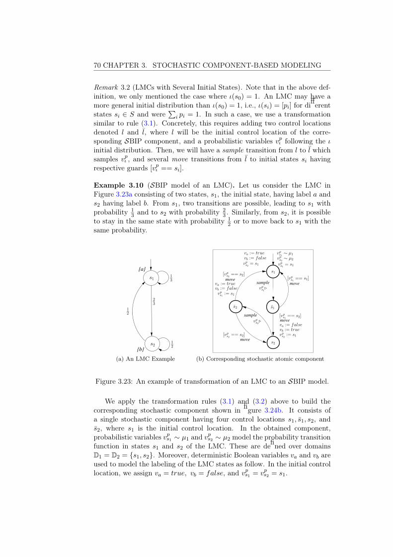
70 CHAPTER 3. STOCHASTIC COMPONENT-BASED MODELING
Remark 3.2 (LMCs with Several Initial States). Note that in the above def-inition, we only mentioned the case where ι(s0) = 1. An LMC may have amore general initial distribution than ι(s0) = 1, i.e., ι(si) = [pi] for differentstates si ∈ S and were
�i pi = 1. In such a case, we use a transformation
similar to rule (3.1). Concretely, this requires adding two control locationsdenoted l and l̄, where l will be the initial control location of the corre-sponding SBIP component, and a probabilistic variables vpι following the ιinitial distribution. Then, we will have a sample transition from l to l̄ whichsamples vpι , and several move transitions from l̄ to initial states si havingrespective guards [vpι == si].
Example 3.10 (SBIP model of an LMC). Let us consider the LMC inFigure 3.23a consisting of two states, s1, the initial state, having label a ands2 having label b. From s1, two transitions are possible, leading to s1 withprobability 1
3 and to s2 with probability 23 . Similarly, from s2, it is possible
to stay in the same state with probability 12 or to move back to s1 with the
same probability.
{a}
{b}
23
s2
s1
12
13
12
(a) An LMC Example
sample
sample
move
move
move
move
[vps2 == s2]
vps1�
[vps1 == s1]
[vps2 == s2]
s̄1s̄2
s2
s1
vps2 = s1 vps1 = s1
vps1 := s1
[vps1 == s2]
va := falsevb := truevps2 := s1
vps2�
va := truevb := false
vps1 ∼ µ1
vps2 ∼ µ2
va := truevb := false
(b) Corresponding stochastic atomic component
Figure 3.23: An example of transformation of an LMC to an SBIP model.
We apply the transformation rules (3.1) and (3.2) above to build thecorresponding stochastic component shown in figure 3.24b. It consists ofa single stochastic component having four control locations s1, s̄1, s2, ands̄2, where s1 is the initial control location. In the obtained component,probabilistic variables vps1 ∼ µ1 and vps2 ∼ µ2 model the probability transitionfunction in states s1 and s2 of the LMC. These are defined over domainsD1 = D2 = {s1, s2}. Moreover, deterministic Boolean variables va and vb areused to model the labeling of the LMC states as follow. In the initial controllocation, we assign va = true, vb = false, and vps1 = vps2 = s1.

CHAPTER 3. STOCHASTIC COMPONENT-BASED MODELING 71
From location s1, a sample transition associated with vps1 leads to s̄1from which a move transition to location s1 or s2 is performed dependingon the outcome of vps1 (s1 or s2). When moving to s2, variables va is set tofalse, vb is set to true, and vps2 is set to s1. The same behavior is replicatedfrom location s2, that is, a sample transition associated this time with vps2and leading to s̄2 is performed. This is followed by a move transition to s1or s2 depending on the valuation of vps2 (s1 or s2). When moving to locations1, va is set to true, vb is set to false, and vps1 is set to s1.
The SBIP component Bs obtained by the construction in Definition 3.12is an LMC MBs
. While in general SBIP models have an MDP semantics,relying on disjoint guards to capture the original model purely stochasticbehavior, prevents any non-determinism and produces an LMC semantics.
Obviously, the state space engendered by this component is bigger thanthe original state space of M. This is due to locations {s̄ ∈ L}, added foreach state s /∈ DetM(S). Therefore, the state space of MBs
grows linearlywhen compared to the original state space. Nevertheless, MBs
is equivalentto M, when observing the relevant set of atomic propositions.
To prove the statement above, let us first take a look to the paths gen-erated by MBs
. These are of the form r = s −→ s̄ −→ s� −→ . . ., wheres = (l;Xp;X). The corresponding traces are of the form σ = (Xp;X) −→(X �p;X) −→ (X �p, X �) −→ . . ., that is, a succession of two steps, the first is asampling of probabilistic variables and the second is a deterministic update.Whereas probabilities of probabilistic steps are given by π(s, s�), the tran-sition probability function of M as specified by the transformation above,deterministic steps have a probability one, hence they do not contribute onthe probability of the generated transition.
When considering Example 3.10 above, one should note that sampletransitions from s to s̄ induces two transitions (since vps1 is defined over D1).For instance, the sample transitions from s1 to s̄1 induces transitions fromstate (s1; (s1, s1); (t, f)) to states (s̄1; (s1, s1); (t, f)) and (s̄1; (s2, s1); (t, f))respectively with probabilities 1
3 and 23 . Similarly, the one from s2 to s̄2 gen-
erates two transitions from state (s2; (s2, s1); (f, t)) to states (s̄2; (s2, s1); (f, t))and (s̄2; (s2, s2); (f, t)) with the same probability 1
2 . This behavior is shownin Figure 3.24a, which gives a clear idea about the type of traces that theSBIP component may generate. For instance,
– σ1 = ((s1, s1); (t, f))23−→ ((s2, s1); (t, f)) −→ ((s2, s1); (f, t)) −→ . . .,
when vps1 evaluates to s2 on transition sample from s1 to s̄1, and
– σ2 = ((s1, s1); (t, f))13−→ ((s1, s1); (t, f)) −→ ((s1, s1); (t, f)) −→ . . .,
when vps1 evaluates to s1 on the same transition.
Coming back to the equivalence statement. Given the generated traces,it suffices to specify the set of observable atomic propositions to be theone of M. This is because building the corresponding stochastic atomic
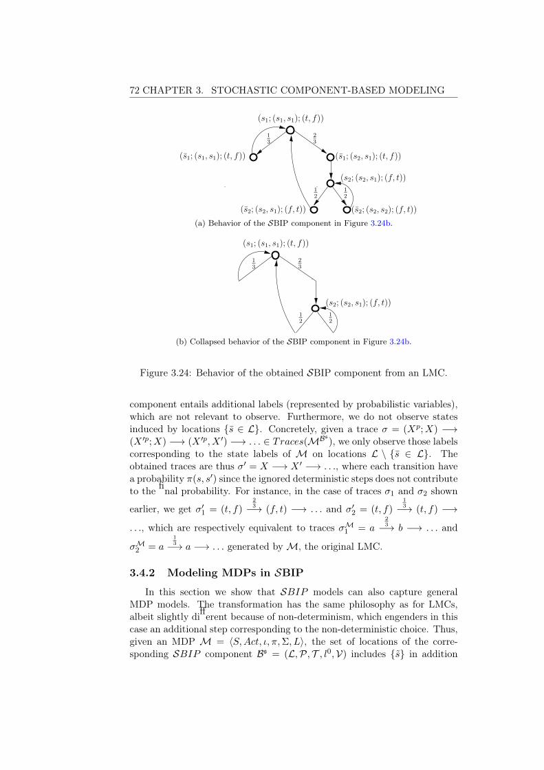
72 CHAPTER 3. STOCHASTIC COMPONENT-BASED MODELING
(s1; (s1, s1); (t, f))
13
23
(s̄2; (s2, s2); (f, t))
(s̄1; (s2, s1); (t, f))(s̄1; (s1, s1); (t, f))
(s2; (s2, s1); (f, t))
(s̄2; (s2, s1); (f, t))
12
12
(a) Behavior of the SBIP component in Figure 3.24b.
(s1; (s1, s1); (t, f))
13
23
(s2; (s2, s1); (f, t))
12
12
(b) Collapsed behavior of the SBIP component in Figure 3.24b.
Figure 3.24: Behavior of the obtained SBIP component from an LMC.
component entails additional labels (represented by probabilistic variables),which are not relevant to observe. Furthermore, we do not observe statesinduced by locations {s̄ ∈ L}. Concretely, given a trace σ = (Xp;X) −→(X �p;X) −→ (X �p, X �) −→ . . . ∈ Traces(MBs
), we only observe those labelscorresponding to the state labels of M on locations L \ {s̄ ∈ L}. Theobtained traces are thus σ� = X −→ X � −→ . . ., where each transition havea probability π(s, s�) since the ignored deterministic steps does not contributeto the final probability. For instance, in the case of traces σ1 and σ2 shown
earlier, we get σ�1 = (t, f)
23−→ (f, t) −→ . . . and σ�
2 = (t, f)13−→ (t, f) −→
. . ., which are respectively equivalent to traces σM1 = a
23−→ b −→ . . . and
σM2 = a
13−→ a −→ . . . generated by M, the original LMC.
3.4.2 Modeling MDPs in SBIP
In this section we show that SBIP models can also capture generalMDP models. The transformation has the same philosophy as for LMCs,albeit slightly different because of non-determinism, which engenders in thiscase an additional step corresponding to the non-deterministic choice. Thus,given an MDP M = �S,Act, ι,π,Σ, L�, the set of locations of the corre-sponding SBIP component Bs = (L,P, T , l0,V) includes {s̃} in addition

CHAPTER 3. STOCHASTIC COMPONENT-BASED MODELING 73
to S and {s̄} previously. Moreover, locations, are identified using actionsnames when several actions are enabled from a given state. The set of portsof the component is obtained by the set Act of M plus additional Act and{sample}. Deterministic variables are obtained from the state labels asfor LMCs, while probabilistic ones are induced from probabilistic distribu-tions associated with the MDP actions. Finally, Bs transitions are of threetypes, corresponding respectively to a non-deterministic step (labeled with�̄ ∈ Act), followed by a probabilistic step (labeled with sample), and finallythe actual move to the successor state (labeled with � ∈ Act). Formally,
Definition 3.13 (Syntactic Transformation of MDPs to SBIP). Given anMDP M = �S,Act, ι,π,Σ, L�, we define the syntactic transformation fromM to a stochastic atomic component Bs = (L,P, T , l0,V) as follows:
– L = S ∪ {(s̄×Act) for each s /∈ ProbM(S)} ∪ {(s̃×Act) for each s /∈DetM(S)},
– l0 = s0, such that ι(s0) = 1,– P = Act ∪ Act ∪ {sample} is the set of ports,– V = Vd ∪ Vp, where Vd = {vap for each ap ∈ AP} and Vp = {vps,� for
each s /∈ ProbM(S) and s /∈ DetM(S) | ∀s� �-successor of s, µs : S ⊂D → [0, 1] and µs,�(s
�) = π(s, �, s�)} ∪ {vps for each s ∈ ProbM(S) and s /∈DetM(S) | ∀s� �-successor of s, µs : S ⊂ D → [0, 1] and µs(s
�) =π(s, �, s�)},
– T contains transition of the form (s, prt, g, (fd, fp), s�), where s, s� ∈L, prt ∈ P, g is defined over Bool(V), and fd and fp are respectivelythe deterministic and probabilistic update functions, such that,
s�−→ s� ∈ π, such that |Act(s)| > 1 and π(s, �, s�) < 1
(s, �̄, true, ∅, (s̄, �)), ((s̄, �), sample, true, (∅, vps,�), (s̃, �)),((s̃, �), �, vps,� == s�, (�(s, s�), ∅), s�) ∈ T
(3.3)
s�−→ s� ∈ π, such that |Act(s)| > 1 and π(s, �, s�) = 1
(s, �̄, true, ∅, (s̄, �)), ((s̄, �), �, true, (�(s, s�), ∅), s�) ∈ T (3.4)
s�−→ s� ∈ π, such that |Act(s)| = 1 and π(s, �, s�) < 1
(s, sample, true, (∅, vps), (s̃, �)),((s̃, �), �, vps == s�, (∅,�(s, s�)), s�) ∈ T
(3.5)
s�−→ s� ∈ π, such that |Act(s)| = 1 and π(s, �, s�) = 1
(s, �, true, (�(s, s�), ∅), s�) ∈ T (3.6)
In the previous definition, one can distinguish two general cases withrespect to the type of the transition to deal with in the given MDP. Thefirst situation is when the transition label is the unique enabled action �from state s, that is, Act(s) = {�}. This corresponds to Rules (3.5) and(3.6) illustrated respectively in Figures 3.25d and 3.25e. In such case, wehave almost the same rules for building an LMC transition (see Figure 3.22cand 3.22b), since there is no non-determinism. With the difference of the

74 CHAPTER 3. STOCHASTIC COMPONENT-BASED MODELING
{a,b}
{b}
s
s�
π(s, �, s�)�
(a) An MDP transition
sample
va := false�
�̄
s̄, �
s̃, �
s
s�
va := truevb := true
vps,��
[vps,� == s�]
(b) Rule (3.3)
�̄
s̄, �
s
s�
va := truevb := true
�va := false
(c) Rule (3.4)
sample
va := false�
s̃, �
s
s�
va := truevb := true
[vps == s�]
vps�
(d) Rule (3.5)
s
s�
va := false
�
va := truevb := true
(e) Rule (3.6)
Figure 3.25: Transformation rules of MDPs to SBIP model.
ports names here given by the MDP actions. The second case is when thetransition is labeled with an action, which is one among many other enabledfrom the corresponding state s, that is, |Act(s)| > 1. In this case, there aretwo possible situations. Depending whether the transition have a probabilityone (deterministic) or not, Rule (3.3) or (3.4) is applied. The first, have anon-deterministic step from s to (s̄, �) followed by a probabilistic step from(s̄, �) to (s̃, �), and finally a deterministic step from (s̃, �) to s�, while thesecond does not have a probabilistic step and moves directly from (s̄, �) tos� as shown in Figures 3.25b and 3.25c.
Example 3.11 (Transforming MDPs to SBIP Components). Figure 3.26ashows an MDP M consisting of states S = {s1, s2, s3} labeled respec-tively by atomic propositions a, c, and b. Form s1, the initial state, a non-deterministic choice exists between actions � and ς, i.e., Act(s1) = {�, ς},where π(s1, �, s1) = 3
4 , π(s1, �, s2) = 14 and ,π(s1, ς, s3) = 1. From states
s2 and s3, only purely probabilistic choice exists, i.e., Act(s2) = {κ} andAct(s3) = {ϑ}, where π(s2,κ, s2) = 1, π(s3,ϑ, s3) =
12 , and π(s3,ϑ, s2) =
12 .
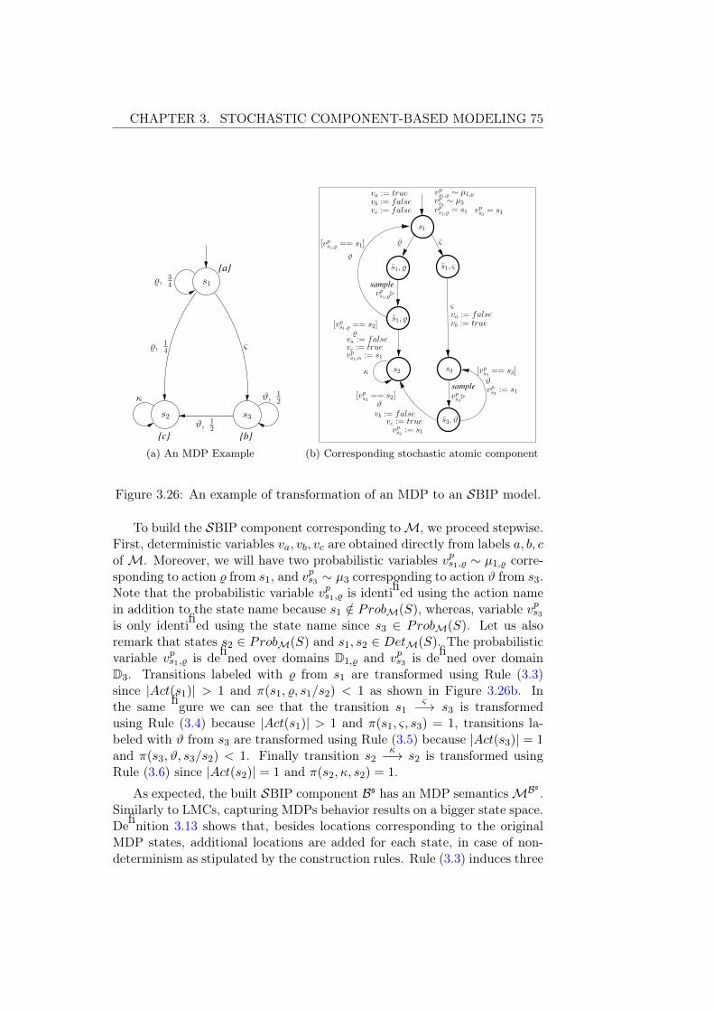
CHAPTER 3. STOCHASTIC COMPONENT-BASED MODELING 75
{b}{c}
{a}
ϑ, 12
s1
�, 14
ς
ϑ, 12κ
�, 34
s3s2
(a) An MDP Example
sample
sample
s1
va := truevb := falsevc := false
ςva := falsevb := true
s3
s̃3,ϑ
vps3�
vps1,��
[vps1,� == s1]
�
vps1,� = s1
ς̄
s̄1, � s̄1, ς
s̃1, �
s2
vps1,� ∼ µ1,�vps3 ∼ µ3
vc := truevb := false
[vps3 == s2]ϑ
vps3 := s1ϑ
�̄
κ
vps3 := s1
[vps1,� == s2]�
va := falsevc := truevps1,α := s1
[vps3 == s3]
vps3 = s1
(b) Corresponding stochastic atomic component
Figure 3.26: An example of transformation of an MDP to an SBIP model.
To build the SBIP component corresponding to M, we proceed stepwise.First, deterministic variables va, vb, vc are obtained directly from labels a, b, cof M. Moreover, we will have two probabilistic variables vps1,� ∼ µ1,� corre-sponding to action � from s1, and vps3 ∼ µ3 corresponding to action ϑ from s3.Note that the probabilistic variable vps1,� is identified using the action namein addition to the state name because s1 /∈ ProbM(S), whereas, variable vps3is only identified using the state name since s3 ∈ ProbM(S). Let us alsoremark that states s2 ∈ ProbM(S) and s1, s2 ∈ DetM(S). The probabilisticvariable vps1,� is defined over domains D1,� and vps3 is defined over domainD3. Transitions labeled with � from s1 are transformed using Rule (3.3)since |Act(s1)| > 1 and π(s1, �, s1/s2) < 1 as shown in Figure 3.26b. Inthe same figure we can see that the transition s1
ς−→ s3 is transformedusing Rule (3.4) because |Act(s1)| > 1 and π(s1, ς, s3) = 1, transitions la-beled with ϑ from s3 are transformed using Rule (3.5) because |Act(s3)| = 1and π(s3,ϑ, s3/s2) < 1. Finally transition s2
κ−→ s2 is transformed usingRule (3.6) since |Act(s2)| = 1 and π(s2,κ, s2) = 1.
As expected, the built SBIP component Bs has an MDP semantics MBs.
Similarly to LMCs, capturing MDPs behavior results on a bigger state space.Definition 3.13 shows that, besides locations corresponding to the originalMDP states, additional locations are added for each state, in case of non-determinism as stipulated by the construction rules. Rule (3.3) induces three

76 CHAPTER 3. STOCHASTIC COMPONENT-BASED MODELING
locations for each state in the MDP enabling non-deterministic and proba-bilistic choices, while Rule (3.6) induces one location for each state enablingpurely deterministic choice. Finally, Rules (3.4) and (3.5) induce two loca-tions for each state in the MDP. All these cases engender a stochastic atomiccomponent with linearly bigger state space. Nonetheless, several generatedstates does not bring useful information and thus will be ignored as forLMCs. Concretely, we only consider states induced by locations L \ {s̄∪ s̃}.Furthermore, we only observe deterministic variables corresponding to theMDP labels. Hence, we can follow the same procedure for LMCs and observethat MBs
is structurally equivalent to the original MDP M.
(s1; (s1, s1); (t, f, f))
p�2
p2
(s2; (s2, s1); (f, f, t))
((s̄1, �); (s1, s1); (t, f, f))
(s3; (s1, s1); (f, t, f))((s̃1, �); (s1, s1); (t, f, f))
((s̄1, ς); (s1, s1); (t, f, f))p1
((s3,ϑ); (s1, s3); (f, t, f))((s3,ϑ); (s1, s2); (f, t, f))
p�1((s̃1, �); (s2, s1); (t, f, f))
(a) Corresponding stochastic atomic component behavior.
(s1; (s1, s1); (t, f, f))
(s2; (s2, s1); (f, f, t))
(s3; (s1, s1); (f, t, f))
κ
ς
ϑ, 12
�, 34
�, 14
ϑ, 12
(b) Corresponding stochastic atomic component collapsed behavior.
Figure 3.27: Behavior of the obtained SBIP component from an MDP.
For instance, when considering Example 3.11, the induced behavior of Bs
in Figure 3.26b is given in Figure 3.27a. This shows the potential traces thatmay be generated when executing Bs. For instance, given a run (s1; (s1, s1);
(t, f, f)) −→ ((s̄1, �); (s1, s1); (t, f, f))34−→ ((s̃1, �); (s1, s1); (t, f, f)) −→ (s1;
(s1, s1); (t, f, f)) −→ . . ., the associated trace when observing all the states
and variables is σ = ((s1, s1); (t, f, f)) −→ ((s1, s1); (t, f, f))34−→ ((s1, s1);
(t, f, f)) −→ ((s1, s1); (t, f, f)) −→ . . ., whereas, if we only observe the spec-

CHAPTER 3. STOCHASTIC COMPONENT-BASED MODELING 77
ified set of states and variables we obtain σ� = (t, f, f)34−→ (t, f, f) −→ . . .,
which is equivalent to the trace σM = a34−→ a −→ . . . of the original MDP.
3.5 Conclusions
The proposed stochastic extension of the BIP formalism enables build-ing stochastic models in a component-based fashion, that is, in an itera-tive and incremental way as explained in [24]. It allows for capturing non-deterministic as well as purely stochastic behaviors by using priorities andschedulers.
We draw the reader’s attention that in this work, we are not concernedwith finding an optimal scheduler given certain requirements as in [108]. Thisis a separate problem that has its own challenges and is out of the scope ofthis dissertation. Our concern here is, to build a purely stochastic SBIPmodel, and to use SMC to analyze it with respect to different properties ofinterest.
As stated in the beginning of the previous section, our stochastic exten-sion inherits BIP expressiveness. We have shown how straightforward it is tomodel MDPs or LMCs using the SBIP formalism. This have been alreadyused in many case studies covering a multitude of domains such as ran-domized distributed protocols [165], automotive [147, 146], avionics [25, 27],many-cores embedded systems [163], multimedia [178], etc. Although, werecognize some limitations and possible amelioration discussed in more de-tails in the conclusion of the dissertation. For instance,
– The size of the induced state space when modeling MDPs or LMCSin SBIP is significant. However, this is not an issue in the context ofthis work since analysis using SMC do not require to build the wholestate space and store it. Furthermore, in the next chapter, we proposea technique aiming to reduce state space size and hence to improve theperformance of SMC.
– Uniform schedulers to resolve non-determinism is the default choice wemade and the easiest to implement. Other alternatives enabling theuse of different probability distributions is discussed in the perspectivesection of the conclusion of the dissertation.
– Currently, SBIP allows only to capture discrete time models. Nonethe-less, it may be extended to cover continuous time by allowing contin-uous data domains for example. We speculate that this will have aGeneralized Semi Markov Process (GSMP) semantics.
– For now, we capture MDPs and LMCs behaviors in a single BIP com-ponent. What would be interesting is to capture it over several SBIPcomponents. This is quite challenging because it will need to synthe-size the corresponding glue.

78 CHAPTER 3. STOCHASTIC COMPONENT-BASED MODELING
From the application perspective, one may ask where to find the proba-bility distributions to be used in the model under construction. The originof such distributions depends on the application domain of the system tobe modeled. For instance, this work focuses on the design of manycore em-bedded systems. In Chapter 6, we present an approach based on statisticalinference to learn probability distributions for the SBIP model. Before reach-ing that point, in the next chapter, we introduce an abstraction techniqueaiming to improve statistical model checking scalability.

Chapter 4Stochastic Abstraction
In the previous chapters, we recalled the probabilistic model checking(PMC) setting and we saw that it is recognized among the most success-ful approaches for quantitative analysis of stochastic models. We discussedthe two main techniques that implement it (numerical and statistical) withmore focus on SMC, which we are adopting in this work for system-level per-formance evaluation. These are shown to be more efficient handling biggermodels, since relying on simulation and statistics.
In spite of its wide use and acceptance, probabilistic model checking tech-niques still encounters significant difficulties when used on real-life systems.First, the stochastic modeling of these systems might be extremely cumber-some. Actually, high expertise is generally required to produce any kind ofmeaningful formal model. For stochastic models, besides functional aspects,they must include stochastic information in form of probabilities. These arehardly available and usually incomprehensible by an average system designer.
Second, whenever such stochastic models exist, they can be very detailedand contain too much information than actually needed for analysis purposes.This is usually the case when stochastic system models are automaticallygenerated from higher level descriptions, e.g., as part of various design flows[22]. For instance, in the case of SMC, Monte-Carlo simulation becomesproblematic as individual simulation time (time to obtain a single executiontrace) could be very long. Henceforth, it could not be possible to obtain anybut only a limited number of traces and consequently, prevent the use ofSMC techniques 1. Moreover, it is worth mentioning that for verification ofsystem-level properties, the observation of any such trace in detail is rarelyneeded. Most of the time, such properties are expressed in terms of fewobservable actions/states of the system while the remaining are completelyirrelevant and can be safely ignored.
1. Similarly, numerical techniques could not be applied in such settings because ex-haustive exploration will not be feasible due to size of the generated models.
79

80 CHAPTER 4. STOCHASTIC ABSTRACTION
In this chapter, we aim at improving the general applicability of proba-bilistic model checking, especially the SMC technique which will be used inthe next part of the dissertation for system-level performance analysis. Tothis end, we propose the combined use of projection and machine learningtechniques to automatically construct faithful abstractions of system mod-els and therefore to overcome the issues discussed earlier. To decide on theappropriate level of abstraction to produce, we suggest using the propertiesunder verification as a guide.
Nowadays, machine learning is an active field of research and learningalgorithms are constantly developed and improved in order to address newchallenges and new classes of problems (see [202] for a recent survey ongrammatical inference). In our context, learning is combined with projectionas follows. Given a property of interest and a (usually large) sample ofpartial traces generated from a concrete system (or system model), we firstuse projection to restrict the amount of visible information on traces tothe minimum required to evaluate the property and then, use learning toconstruct an abstract, probabilistic model which conforms to the abstractedsample set. Under some additional restrictions detailed later in this chapter,the resulting model is a sound abstraction of the concrete model, in thesense that the probability to satisfy the property is approximately the samein the learned and the original model. Hence, it can be used to correctlypredict/generate the entire abstract behavior of the system, in particular, asan input model for SMC.
The above approach has multiple benefits. First of all, the sample set oftraces can be generated directly from an existing black-box implementationof the system, as opposed to a concrete detailed model. In many practicalsituations, such detailed system models simply do not exist and the costfor building them using reverse-engineering could be prohibitive. In suchcases, learning provides an effective, automated way to obtain a model andto get some valuable insight on the system behavior. The use of projectionis also mostly beneficial. In most of the cases, the complexity of the learningalgorithms as well as the complexity of the resulting models are directlycorrelated to the number of distinct observations of traces. Moreover, undernormal considerations, a larger alphabet requires a larger size for the sampleset. Intuitively, the more complex the final model is, the more traces areneeded to learn it correctly. Nevertheless, one should mention that a bit ofcare is needed to meaningfully combine projection and learning. That is,projection may change a deterministic model into a non-deterministic one,and henceforth has an impact on the learning algorithms needed for it.
We start the chapter by a brief reminder of some probabilistic model-ing and learning techniques. Then, we detail the joint use of projection andlearning as a method to compute an appropriate system abstraction for anal-ysis. The convergence and the correctness of the proposed method are thendiscussed and assumptions are clearly stated. We finally show the concrete

CHAPTER 4. STOCHASTIC ABSTRACTION 81
use of the method on Herman’s Self Stabilizing Algorithm with an increasingnumber of processes, before concluding the chapter and presenting a benchof related works.
4.1 Preliminaries
We first recall and define some important notions for the forthcomingdevelopment. We mainly recall the concept of determinism in the contextof LMCs. We also provide a definition for probabilistic automata as analternative model for stochastic systems. These are also the models that mostof the learning algorithms were designed for. Finally, we give an overview ofprobabilistic learning techniques.
4.1.1 Additional Stochastic Models
Probabilistic Finite Automata
Probabilistic finite automata (PFA) represent an alternative for modelingprobabilistic systems. They are defined similarly to LMC with the differenceof having termination states.
Definition 4.1. (Probabilistic Finite Automata) The probability transitionfunction π is now defined on S×S ∪ {$} and π(s, $) stands for the probabilityto terminate execution at state s. Henceforth, the associated notions ofpaths and traces correspond to finite paths and finite traces for an LMC.The probability of a finite path r = s0s1...sn of a PFA is
P (r) = ι(s0) · (n−1�
i=0
π(si, si+1)) · π(sn, $).
Deterministic PFA are defined similarly to DLMCs and are denoted asDPFA.
4.1.2 Probabilistic Learning Techniques
Learning probability distributions over traces is a hard problem [76] withpotential applications in a wide range of domains, far beyond formal veri-fication. Many methods have been proposed in the research literature andare continuously improved and challenged on learning research competitions[202]. The family of state merging techniques is one of the most success-ful nowadays. Intuitively, these techniques proceed by first constructingsome large automata-based representation of the set of input traces andthen progressively compacting them, by merging states, into a smaller au-tomaton, while preserving as much as possible trace occurrence frequen-cies/probabilities. Different algorithms in this family can learn either DPFAmodels [54, 78, 77] or general PFA models [193, 180, 81].

82 CHAPTER 4. STOCHASTIC ABSTRACTION
The AAlergia Algorithm
AAlergia [153] is a state merging algorithm that exclusively learn de-terministic models. It is a variant of the Alergia algorithm [54] proposedby Carrasco and Oncina in early nineties. Given a sample of traces, thealgorithm proceeds in three steps, as depicted in Figure 4.1.
Step 1: it builds an intermediate representation, named Frequency Pre-fix Tree Acceptor (FPTA), which is a restricted form of DPFA thatrepresents all the traces in the input sample and their correspondingfrequencies (number of occurrence in the sample).
Step 2: based on a compatibility criterion parametrized by αA (see [153]for details), it iteratively merges states of the FPTA having the samelabels and similar probability distributions until reaching a compactDPFA.
Step 3: it transforms the obtained DPFA into a DLMC model by normal-izing the probabilities of termination.
Step 3Step 2 DLMCA sample of N traces
Step 1FPTA DPFA
αA
Figure 4.1: Main steps of the AAlergia algorithm.
AAlergia is proven to converge to the correct model in the limit 2 if theinput traces are generated randomly, and with random lengths, from anLMC model [153]. A first consequence concerns verification on DLMCs andensures that, in the limit, a given LTL property will hold on the original andthe learned model with approximately the same probability. This result ispartially extended to LMC. That is, for arbitrary Markov chain models, thealgorithm might not converge to the good model in general. In the case ofinput traces from a non-deterministic LMC model (which moreover, does nothave an equivalent deterministic representation), as the sample size increases,AAlergia will build a sequence of DLMCs (usually, of increasing size) tendingto approximate the original model. It is proven that, in the limit, theselearned DLMC models provide an increasingly better approximation for theinitial (prefix) behavior, and hence preserve the satisfaction of bounded LTLproperties.
2. When the sample size tends to be infinite, the learned model converges to the originalsystem. This is known as identification in the limit and is widely used in grammaticalinference [99].

CHAPTER 4. STOCHASTIC ABSTRACTION 83
4.2 Abstraction via Learning and Projection
The verification problem in the stochastic setting amounts to computeP (M |= ϕ) for an LMC model M and an LTL property ϕ. In several cases,M is not explicitly known, that is, it could be a black-box probabilisticsystem which can be executed arbitrarily many times in order to producearbitrarily long traces. As stated in the introduction of the chapter, produc-ing any stochastic system model is inherently difficult. Moreover, decidingon the appropriate level of abstraction of the model, that is, the amount ofdetails to model/ignore, is an open question and is quite challenging. Finally,the verification complexity is proportional to the produced model size.
Due to these reasons, we would like to avoid the verification of ϕ onthe original model M. Instead, we would like to perform it on a smaller,abstract model M� which preserves the satisfaction probability of ϕ, that is,P (M |= ϕ) = P (M� |= ϕ). We propose hereafter a method to compute suchan abstraction M� by combining learning and a projection operator on tracesparametrized by the property ϕ. The idea is based on the observation that,when checking a model against a property, only a subset of the propositionsis really relevant. In fact, only the atomic propositions mentioned explicitlyin the property are useful while the others can be safely ignored.
The proposed approach is depicted in Figure 4.2. It consists of initiallygenerating a finite set of random finite traces T (with random lengths) fromM (the sampling operation). In a second step, a projection is applied ontraces T in order to restrict the atomic propositions to the ones needed forthe evaluation of the property ϕ. The projection is guided by the propertyϕ as detailed below. Third, the set of projected traces is used as an inputto a learning algorithm. For the experiments, we will use the AAlergiaalgorithm [153], however, any other algorithm could be used. The outputof the learning step denoted M� on Figure 4.2 will be used to evaluate theproperty of interest ϕ.
traces(Learning)(Execution)
(Learning)traces
(Relabeling)
(Execution)
T M �
Ta (M� ≈ Ma)
(M� ≈ M)
M�
(Projectionϕ)
M = �S, τ,π,Σ, L�
Ma = �S, τ, π,Σ, La�
Figure 4.2: Illustration of our approach for learning abstract models.
It is worthwhile to mention that, in our approach, the sampling step(which could be time consuming depending on the used sample size) is doneonly once, while the following steps (projection and learning) are repeatedgiven different properties 3. Our approach ensures a significant time reduc-
3. This is not always need as will be shown later. Basically, we redo projection onlyfor those classes of properties that have different sets of symbols.

84 CHAPTER 4. STOCHASTIC ABSTRACTION
tion with respect to applying SMC directly on the black-box system sinceit generally requires trace re-sampling every time. In [188], a method isproposed to avoid re-sampling in a slightly different setting, but it raisesconfidence issues as discussed in the related work section at the end of thechapter. In addition, some SMC algorithms, besides their termination guar-antee, might potentially need a huge number/length of traces depending onthe required confidence level.
The proposed approach is sound under some conditions. Note that aprojection may potentially introduce non-deterministic behavior at the levelof traces. Consequently, we need to distinguish several cases. The first oneis when the traces are generated from a DLMC and the projection operationdoes not introduce any non-determinism. In this case any learning algorithm,for instance AAlergia, works. Another case is when the traces are generatedfrom an LMC and/or the projection introduces non-determinism. This caseis divided into two sub-cases depending on the type of non-determinism.If the non-deterministic model has an equivalent deterministic one, thenany learning algorithm can be used. Otherwise, one needs to use learningalgorithms capable to learn non-deterministic models such as [193, 81].
Next, we detail the main steps of the approach and illustrate them onthe Craps Gambling Game example. The correctness is formally establishedby Theorem 4.1.
4.2.1 Abstraction Steps
In this subsection, we illustrate the different steps of the abstractionapproach on the Craps Gambling Game model presented in Chapter 2. Wefirst define the projection operation and depict the learning phase using theAAlergia algorithm. We then show the learned models obtained for twoexample properties. Finally, we provide verification results on the obtainedmodels using SMC.
Projection
The projection operation is defined on sample traces generated from thestochastic system, so as to reduce the number of labels and henceforth, lateron, the number of states in the learned model. In this work, we introducea first syntactic definition of a projection operator. It intuitively consists ofignoring the atomic propositions that are not relevant to the property underverification as formally defined below.
Definition 4.2. Given a property ϕ, we define Vϕ ⊆ AP the support of ϕas the set of atomic propositions occurring explicitly in ϕ.
Definition 4.3. The projection operator Pϕ : Σ∗ → Σ∗ is defined as
Pϕ(σ0σ1...σn) = σ�0σ
�1...σ
�n

CHAPTER 4. STOCHASTIC ABSTRACTION 85
where σ�i = σi ∩ Vϕ for all i ∈ [0, n].
Given the definitions above, one can easily see that for two differentproperties ϕ1 and ϕ2, the projection operation may produce the same setof traces, if they have the same support, that Vϕ1 = Vϕ2 . We define a classof properties as the set of properties that have the same support. For suchproperties, the projection and learning steps are required once. Furthermore,if the support of ϕ1 is only a subset of ϕ2 (Vϕ1 ⊂ Vϕ2), then the learned modelgiven ϕ2 may be used to verify both properties.
Example 4.1 (Projection on the Craps Gambling Game Traces). Given aset T of traces generated from the Craps Gambling Game model in Fig-ure 2.1 and the properties ϕ1 = F won and ϕ2 = F (won ∨ lost), we applyDefinitions 4.2 and 4.3 respectively to compute the corresponding supportsVϕ1 = {won}, Vϕ2 = {won, lost} and the sets of projected traces Ta1 andTa2 below.
– T = {start won, start lost lost, start won won won won won won wonwon won, start point5, start point10 point10 point10 point10 point10,start point9 point9, . . .};
– Ta1 = {τ won, τ τ τ , τ won won won won won won won won won,τ τ , τ τ τ τ τ τ , τ τ τ , . . .};
– Ta2 = {τ won, τ lost lost, τ won won won won won won won won won,τ τ , τ τ τ τ τ τ , τ τ τ , . . .}
Learning
We briefly illustrate the learning phase using AAlergia on the runningexample. Figure 4.3 shows three abstract models of the Craps GamblingGame obtained from the set T of 5000 traces generated from the model inFigure 2.1 (partially presented in Example 4.1). One can note from this figurethe important reduction of the sizes of the obtained models with respect tothe original one. Figure 4.3a shows the model learned by AAlergia takingas input the set Ta2 , that is, with respect to property ϕ2 = F (won ∨ lost).Figure 4.3b is obtained by applying AAlergia on the set Ta1 , that is, projectedwith respect to ϕ1 = F won. Remark that this model is not equivalent butonly an approximation of the original model in Figure 2.1. That is, in thelatter there exists some non null probability to never reach the won state,whereas, in the learned model the won state is reachable with probability 1.This approximation could however improve if a larger set of traces is usedfor learning as stated in the previous section. Finally, the third learnedmodel shown in Figure 4.3c is equally obtained from Ta1 but when using analgorithm able to learn non-deterministic models such as the one in [193].

86 CHAPTER 4. STOCHASTIC ABSTRACTION
1 1
0.110.67
0.22
0.72
0.170.11
lostwon
S3
S0
S2
τ
S1
τ
(a) Scenario 1
1
0.47 0.53
0.37
0.63
won
S1
S2
τ
S0
τ
(b) Scenario 2
1 1
0.110.67
0.22
0.72
0.170.11
won
S2
S1
τ
S3
τ
S0τ
(c) Scenario 3
Figure 4.3: Learned Abstract Models of the Craps Gambling Game. 4.3aand 4.3b are obtained using AAlergia, while 4.3c is obtained using [193]. Forall of them, we used 5000 traces generated from the model in Figure 2.1 andperformed projection with respect to properties ϕ1 and ϕ2.
Abstract Model Analysis
Once the model is learned, we evaluate the property used for projec-tion on the obtained abstraction. Table 4.1 provides results of verifying theproperty ϕ1 = F won on the obtained Craps Gambling Game models. Itshows that the model in Figure 4.3a exhibits similar probability to the orig-inal Craps Gambling Game model, whereas the one in Figure 4.3b showsa different result. The reason is that the projection performed in this caseintroduced non-determinism in the input sample. In addition, it seems thatin this case there is no equivalent deterministic model that could be learnedby AAlergia. Finally, note that the model in Figure 4.3a is obtained withrespect to ϕ2 having the support Vϕ2 = {won, lost} and that we were ableto use it to verify ϕ1 since Vϕ1 = {won} ⊆ Vϕ2 as explained earlier.
Models P (ϕ1)
Scenario 1(Figure 4.3a) 0.485
Scenario 2 (Figure 4.3b) 1
Original Model (Figure 2.1) 0.493
Table 4.1: Verification results of ϕ1 on the original and the abstract CrapsGambling Game models using SMC (PESTIM).
4.2.2 Correctness Statement
The correctness of our approach is formally stated as follows.

CHAPTER 4. STOCHASTIC ABSTRACTION 87
Theorem 4.1. Let M be an LMC model and let ϕ be an LTL property. LetM� be the learned model from a sample set of size n of traces generated fromM and projected according to ϕ as in Definition 4.3. Then, in the limit, M�
is a correct abstraction for the verification of ϕ, that is
P ( limn→∞
P (M |= ϕ) = P (M� |= ϕ)) = 1
if eitheri) ϕ belongs to the bounded fragment BLTL and the learning algorithm
converges for DLMC models, orii) the learning algorithm converges for arbitrary LMC models.
Proof. First, let us remark that M� is constructed as illustrated by the thickline in Figure 5.1. Let us moreover observe that any sample set of projectedtraces Ta obtained from M is equally obtained from Ma, that is, from the"abstracted" version of M where only the labeling function has changed fromL into La by taking La(s) = L(s) ∩ Vϕ, for all s ∈ S. In other words, theleft-hand side of the diagram shown in Figure 5.1 commutes. Henceforth, Mand Ma are identical with respect to the satisfaction of ϕ. The underlyingset of runs and their associated probabilities are the same in M and Ma.As the atomic propositions occurring in ϕ are preserved by relabeling, itobviously holds that P (M |= ϕ) = P (Ma |= ϕ).
Moreover, learning from the sample set Ta leads eventually to Ma. Thatis, under particular restrictions specific to the learning algorithms and limitconditions, the learned model M� will be an equivalent representation ofMa, that is, M� ≈ Ma. We distinguish two cases depending on the learningalgorithm:
i) In the case of deterministic models learning (e.g., AAlergia), the learnedmodel M� is provable equivalent only for a deterministic input modelMa. But, in addition, for the general case, this models is also pro-viding good approximations for the initial (prefix) behavior of Ma
and hence preserve the probability of satisfaction for properties in theBLTL fragment (see Theorem 3 in [153]). Thereof, by using AAlergiaor a similar learning algorithm, it holds that P (limn→∞ P (Ma |= ϕ) =P (M� |= ϕ)) = 1 whenever ϕ belongs to BLTL.
ii) In the general case of non-deterministic models learning, it is guar-anteed in the limit that Ma ≈ M�. Thereof, one can safely concludethat P (limn→∞ P (Ma |= ϕ) = P (M� |= ϕ)) = 1 for any ϕ.
Henceforth, in both cases it holds that
P ( limn→∞
P (M |= ϕ) = P (M� |= ϕ)) = 1 (4.1)
Table 4.2 summarizes the key results of the abstraction approach. The �symbol identifies the case where the used learning algorithm is only able to

88 CHAPTER 4. STOCHASTIC ABSTRACTION
learn DLMCs (such as AAlergia) and when M is non-deterministic (eitherinherently or because of projection) and ϕ is an LTL property. In general,equality 4.1 does not hold in this scenario. However, when there exists anequivalent deterministic model to M, this may hold.
Learning Algorithm
Converge to a DLMC M� Converge to an LMCM�
M DLMC LMC (D)LMC
ϕ (B)LTL BLTL LTL (B)LTL
Equality 4.1 � � � �
Table 4.2: Summary of the possible settings and the corresponding results.
4.3 Herman’s Self Stabilizing Algorithm
To experiment our approach, we use the Herman’s Self Stabilizing Pro-tocol [111]. The goal of such a protocol is to perform fault tolerance byenabling a distributed system starting in an arbitrary state to converge to alegitimate one in a finite time. Given a token ring network where the pro-cesses are indexed from 1 to M (M must be odd) and ordered anticlockwise,the algorithm operates synchronously. Processes can possess tokens, whichcirculate in one direction around the ring. At every step, each process witha token tosses a coin. Depending on the outcome, it decides to keep it or topass it on to the right neighbor. When a process holds two tokens, they areeliminated. Thus, the number of tokens remains odd. The network is saidto be stable if exactly one process has a token. Once such a configuration isreached, the token circulates forever, fairly, around the ring.
We apply our abstraction approach to several configurations of the pro-tocol (M = {7, 11, 19, 21}). Note that as the number of processes in-creases, the state space becomes very large and makes the verification quiteheavy even using simulation-based methods such as SMC. We use AAler-gia for learning and show that we are able to reduce the state space whilestill accurate for several properties. We consider the bounded propertiesϕL = P (true UL stable) and ψL
M = P (tokenM UL stable) where M is thenumber of processes in the network and L is a bound. The first propertystates that the protocol reaches the stable state in L steps whatever theintermediate ones are. The second specifies in addition that the protocoldirectly moves from M tokens to the stable state (1 token), that is, all thestates before stable are tokenM. We first apply the projection on the tracesgenerated from the different configurations using the properties supportsVϕL = {stable} and VψL
M= {tokenM, stable}. Then, we use AAlergia to
learn the corresponding models shown in Figure 4.4. The models obtained

CHAPTER 4. STOCHASTIC ABSTRACTION 89
for M = {19, 21} are similar to M = 11. Finally, we verify the obtainedabstractions with respect to different instances of the properties ϕL and ψL
M ,that is, for various values of L and M .
1
0.89 0.11
0.2
0.8
stable
S1
S2
τ
S0
τ
(a) Given ϕL
1
0.87 0.11
0.2
0.8
stable
token70.02
S1
S2
τ
S0
(b) Given ψL7
stable
1
0.07
0.93
S0
τ
S1
(c) Given ϕL
stable
token11
0.88
1
0.1190.001
0.922
0.078
S1
S2
τ
S0
(d) Given ψL11
Figure 4.4: Abstract Herman’s Self Stabilizing Protocol models learned usingAAlergia with respect to ϕ and ψ, for M = 7 (a,b) and M = 11 (c,d).
Table 4.3 summarizes the learned models characteristics, AAlergia perfor-mance when combined with projection, and verification results using PRISM[139]. In this table, the first two columns list the used configurations andtheir corresponding sizes. The third column depicts the properties underconsideration. Information about the learning process are then detailed: αA
is the AAlergia compatibility criterion parameter, Size is the learned modelsize, and Time is the learning time in seconds. The last part concerns thecomparison of the original and the learned model in term of properties prob-abilities and verification time. The verification part relies on the PESTIMalgorithm which is parametrized by two confidence parameters δ and α.
The results in Table 4.3 point out two important facts. The first is thedrastic reduction of the learned models sizes and SMC time compared to theoriginal Herman’s Self Stabilizing protocol model. Figure 4.5 summarizes theSMC time of ϕ10 for the learned and the original models when increasingthe number of processes M . Figure 4.5 and the Table 4.3 allow us to seehow big is the SMC time of the original model with respect to the abstractone. Figure 4.5 shows in addition the learning time which is also far belowthe SMC time of the original model for M > 11. Moreover, one can see thatthe time to learn plus the time to verify the abstract model is below theSMC time of the original model for M > 11, which confirms the pertinenceof our approach for big models. For instance, for M = 19, learning takesabout 83 seconds and verification takes about 0.307 seconds while verifyingthe original model takes about 13 hours. Furthermore, since the samplingstep is done only once in our approach, its time impact is reduced whenconsidering many properties. The second fact shown in Table 4.3 is that,

90 CHAPTER 4. STOCHASTIC ABSTRACTION
Size Prop.Learning SMC
δ,αLearned Model Original Model
αA Size Time(s) Prob. Time(s) Prob. Time
M = 7 27
ϕ10 [2−9, 20] 3 69.7010−2, 10−1 0.874 0.180 0.874 3.40 s10−2, 10−2 0.880 0.320 0.873 5.44 s
ψ30 [2−6, 26] 3 45.9810−2, 10−1 0.112 0.050 0.112 0.93 s10−2, 10−2 0.109 0.111 0.111 1.51 s
φ [2−8, 20] 4 167.50 – 0.160 0.005 0.167 0.02 sSample Size = 5000
M = 11 211
ϕ10 [2−4, 26] 2 54.6710−2, 10−1 0.517 0.250 0.543 33.1 s10−2, 10−2 0.518 0.440 0.543 58.3 s
ψ30 [2−6, 26] 3 60.2210−2, 10−1 0.011 0.039 0.012 12.1 s10−2, 10−2 0.012 0.070 0.011 21.7 s
Sample Size = 5000
M = 19 219
ϕ10 [2−4, 26] 2 82.9510−2, 10−1 0.197 0.180 0.148 8.1 h10−2, 10−2 0.191 0.307 0.151 13.3 h
ψ30 [2−6, 26] 3 172.5810−2, 10−1 0.000 0.040 0.0001 5.7 h10−2, 10−2 0.000 0.074 0.0008 10.1 h
Sample Size = 10000
M = 21 221ϕ10 [2−10, 20] 3 253.71
10−2, 10−1 0.169 0.355 0.172 34 h10−2, 10−2 0.163 0.616 − > 5 d
Sample Size = 10000
Table 4.3: Abstraction and verification results of ϕ10 and ψ30 using PESTIM.
besides this reduction, the models are quite accurate in terms of probabilitymeasures as clearly shown in Figures 4.6, 4.7a, and 4.7b as well. Thesefigures show the verification results of ϕL (for different L) on the originalprotocol versus the learned model for all the considered configurations. Forexample, for M = 21, the probability to satisfy ϕ10 is 0.172 for the originalmodel and 0.169 for the learned one, that 3. 10−3 of inaccuracy.
It is worth to mention that the results for M = 21 shown in Figure 4.7bare obtained using the PESTIM algorithm with confidence δ = 5.10−2,α =5.10−3. That is, with less confidence when compared to the results in Table4.3. This choice is made to reduce the experiments time since the goal ofthe figure is to show the global behavior of the learned model with respectto the original one. It was sufficient in this case to take low confidence levelto get very similar shapes.
In addition to PESTIM, we used the SPRT technique to validate withmore confidence the results of the property ψL
M = P (tokenM UL token1) ≥ θfor M = 7, 11. We fixed the confidence parameters to α = β = 10 −3
and δ = 10−3. Table 4.4 shows the verification results and performanceof the SMC algorithm (verification time and number of traces) for differentL values. Note that for this experiment, we used the same model learnedpreviously. In this table, θ is the probability range to satisfy ψL
M , Tracesis the number of traces used by SPRT, and Time is the SMC time. This

CHAPTER 4. STOCHASTIC ABSTRACTION 91
1e
+0
01
e+
02
1e
+0
41
e+
06
Number of processes in Herman's Protocol
Tim
e in
se
co
nd
s
7 11 19 21
SMC Time - Original modelSMC Time - Learned modelLearning Time
Figure 4.5: Statistical Model Checking Time of ϕ10: original vs. abstractHerman’s Self Stabilizing Protocol model. Obtained using PESTIM algo-rithm with δ = 10−2,α = 10−2.
Figure 4.6: ϕL verification results using PESTIM for M = {7, 11}.
table confirms the observation made in the previous experiment, that is,the reduction of the SMC time when using the abstract model while theprobability estimation is still accurate.
Results on Unbounded LTL using Numerical PMC We did an ad-ditional experiment on the Herman’s Self Stabilizing protocol with M = 7in order to investigate the usability of this instance of the approach for un-

92 CHAPTER 4. STOCHASTIC ABSTRACTION
(a) M = 19.
(b) M = 21.
Figure 4.7: ϕL verification results using PESTIM for M = {19, 21}.
bounded LTL properties (all the considered properties so far were bounded).We considered the property φ = P (N(token5 U stable)) which queries themodel with respect to the probability to reach a stable state directly from astate with 5 tokens. N is the Next operator and is used for technical reasons.Since the initial state of the Herman’s Protocol with M = 7 has 7 tokens,we use Next to avoid this state. Otherwise, the probability of φ will be 0.
The learned abstract model corresponding the this experiment is shownin Figure 4.8 and the verification results are depicted in Table 4.3. The

CHAPTER 4. STOCHASTIC ABSTRACTION 93
LOriginal Model Learned Model
θ Traces Time(s) θ Traces Time(s)
M = 7L = 1 [0.109, 0.110[ 622018 25.643 [0.107, 0.108[ 588357 1.363L = 30 [0.111, 0.112[ 622834 25.749 [0.108, 0.109[ 533885 1.282L = 65 [0.111, 0.112[ 651434 26.756 [0.108, 0.109[ 476883 1.118
M = 11L = 1 [0.011, 0.012[ 147178 85.135 [0.012, 0.013[ 163600 0.411L = 30 [0.011, 0.012[ 105362 60.206 [0.013, 0.014[ 098493 0.262L = 65 [0.011, 0.012[ 137469 80.648 [0.013, 0.014[ 248300 0.564
Table 4.4: Statistical Model Checking of ψLM on the original and the learned
Herman’s Self Stabilizing Protocol models. Obtained using the SPRT algo-rithm with α = β = 10 −3, δ = 10−3.
1
0.330.56
0.11
0.789
0.0010.21
stable token5
0.58
0.31
0.11
S3
S0
S2
τ
S1
τ
Figure 4.8: Abstract Herman’s Self Stabilizing Protocol model with M = 7using the AAlergia algorithm. Obtained with respect to property φ.
obtained results show that the probability of satisfying φ is almost the samefor the abstract and the original protocol models. Concretely, we obtained0.160 for the abstract model and 0.167 for the learned one. This is possible(to check unbounded LTL properties on the abstract model with a goodaccuracy) because, in this case, there exist an equivalent deterministic modelfor the original Herman’s Self Stabilizing protocol (which encompasses non-determinism) that AAlergia was able to capture. For the verification part, weused numerical probabilistic model checking algorithm implemented withinPRISM to show that the proposed abstraction method is also beneficial forthis category of algorithms.
4.4 Conclusions and Related Work
Conclusions and Future Work
Reducing the PMC time, and more specifically the SMC time, of a givenLTL property on large stochastic models is the primary benefit of our abstrac-

94 CHAPTER 4. STOCHASTIC ABSTRACTION
tion approach. This gain is achieved through the combined use of projectionon traces and machine learning. Projection is performed by considering thesupport of the property of interest, that is, the set of symbols explicitlyappearing in that property, while learning automatically infers a compactmodel using state merging techniques. The proposed approach could be in-stantiated with any learning algorithm, under the assumption that it respectsthe conditions discussed earlier. It produces accurate models preserving theprobability of satisfying the property of interest. Experimental results showthat (1) verifying the property of interest on the abstract model is faster thandoing it on the original one, and (2) that the estimation of the probabilityof satisfying the properties is accurate with respect to the one obtained onthe original system.
In the current stage of work, the proposed projection definition is quitesimple. It allowed us to instantiate our methodology and to implement itfor validation. As future work, we are planning to improve it to obtaincoarser abstractions, yet preserving the probability of the underlying prop-erty (as opposed to a class of properties currently). This could be potentiallyachieved by taking into account the semantics of the LTL operators. We shallalso apply the approach to other real-life systems and consider using otheralgorithms able to learn non-deterministic models. An important extensionwould be to adopt it for learning SBIP components and their correspond-ing glue. Furthermore, the proposed approach is only applicable to discretestochastic systems. An interesting direction to investigate is its extension tocontinuous systems such as continuous time Markov chains or probabilistictimed automata. We provide hereafter some pertinent works that may helpobtaining such an extension.
Related Work
In this section, we first provide an overview of studies that applied learn-ing techniques for systems verification in general. These are not necessarilystate merging, nor in the limit identification techniques. For more details, werefer the reader to the literature survey by Martin Leucker [148]. With refer-ence to the future research directions mentioned above, we present a benchof algorithms that allow for learning non-deterministic behavior of systemsin addition to probabilities. In the same perspective, we introduce otheralgorithms for learning stochastic continuous-time models such as CTMCsand GSMPs.
Pena et al. propose to use machine learning for the purpose of statereduction in incompletely specified finite state machines (for which for allstates and all inputs, the next state or outputs are unknown) [167]. Themain motivation of this work is that (a) it is proven that the state reductionin incompletely specified finite state machines is NP-complete, and (b) theexact and heuristic existing solutions are time consuming. The authors ap-

CHAPTER 4. STOCHASTIC ABSTRACTION 95
proach the problem using learning techniques to obtain a minimal system forgiven input/output mappings. Based on Angluin’s L* algorithm, which com-putes the minimal DFA in polynomial time, the authors propose a learningtechnique to obtain an equivalent FSM to the given input.
Cobleigh et al. propose to use learning for assumptions generation inassume-guarantee style compositional verification to address state space ex-plosion problem in verification of systems [65]. Verification is achieved inan incremental fashion, that is, an assumption that characterizes a certaincomponent C context is first generated and combined with a property, thenchecked with respect to C. If the assumption is satisfied by C and on the restof the system as well, it is proven that the property is verified on the wholesystem. This iterative process is shown to terminate. In fact, the algorithmconverges to an assumption that is necessary and sufficient for the propertyto hold on the underlying system.
Peled et al. propose to combine model checking, testing, and learning toautomatically check properties of systems whose structure is unknown [166].This paper motivates black-box checking where a user performs acceptancetests and does not have access to the design, nor to the internal structureof the system. The authors, however, conclude that the complexity of theiralgorithms could be reduced if an abstract model of the system would beavailable. Additionally, the authors point out the need to take into accountthe property of interest to tackle verification complexity.
In the same context, (of black-box systems), we also mention the workby Sen et al. which propose an SMC algorithm to verify this kind of sys-tem [188]. In this work, systems are assumed to be uncontrolled, that is,traces cannot be generated on demand. The approach cannot guarantee cor-rect answers within required error bounds. It computes instead a p-value asa confidence measure. In contrast to our approach, [188] uses pre-generatedtraces as direct input to their SMC algorithm. This raises confidence issuesbut makes it faster since no learning is performed.
Habermehl et al. propose to use learning for regular model checkinginfinite-state systems [102]. The learning technique enables generating asample of reachable configurations of the given system. Methods for inferenceof regular languages are used to generalize the sample towards obtaining thefull reachability set or an over-approximation where the property of interestholds.
In the first part of the chapter, we briefly mentioned some algorithms forlearning non-deterministic models such as PFAs. These are all following astate merging approach. Here, we introduce additional algorithms using adifferent technique and detail both categories.
Recently, Mao et al. proposed a new algorithm called IOAlergia to learnMDPs [154] from sample traces, following the same assumptions and pro-cedure in AAlergia [153]. IOAlergia is an adaptation of the Alergia algo-rithm [54] in the context of non-deterministic models, specifically for de-

96 CHAPTER 4. STOCHASTIC ABSTRACTION
terministic labeled MDPS. Stolcke and Omohundro propose a Bayesian al-gorithm for learning the parameters and the structure of Hidden MarkovModels (HMMs) [177] 4 following a state merging fashion [194, 193]. In thiswork, similarly to Alergia, an initial specific representation consisting of thetraining input data is first built. Then, based on Bayesian posterior proba-bility, a more general model is derived by merging states. Ron et al. proposean algorithm for learning a subclass of acyclic PFAs [180]. This work alsouses state merging starting from an initial representation of input traces.The merge criterion is based on frequencist statistics in contrast to the pre-vious Bayesian approach. The above mentioned algorithms are all proven tolearn the correct target model in the limit.
In contrast to the previous merging-based algorithms, more recent work[81, 103] proposes to learn more powerful models 5 such as Multiplicity Au-tomata (MA). These works performs identification of underlying rationallanguages residuals and iteratively solve equations over them.
The previously mentioned works essentially focus on discrete-time mod-els. However, others work, albeit few, exists for learning continuous-timemodels. For instance, Verwer et al. propose to learn Timed Automata (TA)from timed systems observations [203]. The algorithm start by a prefix treeand performs merging and splitting based on hypothesis testing and well-known statistical tests. This work learns models in the deterministic con-text, in the sense of no probabilistic behavior. In the following, we presenttwo algorithms for learning stochastic continuous-timed models. Sen et al.proposed an algorithm to learn CTMCs models from sample traces [187].In this work, the authors follow the state merging approach by providing avariant of the Alergia algorithm. In [79], Pedri et al. propose an algorithmfollowing the same strategy to learn more general continuous-time models,namely GSMPs. This uses new statistical clocks estimators, in addition tothe state compatibility criterion of Alergia.
So far, we presented a set of formalisms and techniques for both prob-abilistic modeling and analysis of stochastic systems. This first part ofthe dissertation could be seen as a stochastic framework for component-based stochastic modeling, automatic stochastic abstraction through ma-chine learning, and stochastic model analysis using probabilistic model check-ing and more specifically, statistical model checking.
In the next part, we will introduce a method for dealing with performanceaspects at system-level in the context of embedded systems design. There, wewill be using our stochastic framework to build functional high-level modelsencompassing performance details and to analyze them with respect to globalextra-functional requirements.
4. These could be seen as PFAs where the strings generation is performed accordingto probability distributions of state symbols.
5. For more details about the classification of the above mentioned models in term ofexpressiveness, we refer the reader to [202].

PART II
METHODS AND FLOW
97


Chapter 5Rigorous System-level Performance
Modeling and Analysis
The first part of the manuscript has set up most of the foundations of thepresent work. It depicted our contributions in terms of formalism for stochas-tic modeling of systems, that is, the SBIP component-based formalism, inaddition to techniques for probabilistic analysis of these systems and theirabstraction. In this second part, we will use these ingredients to construct arigorous approach for system-level performance modeling and analysis of em-bedded systems. The part is split into four chapters. The first introduces theASTROLABE approach and its different steps. In the second chapter, wegive a detailed view on the method we propose for statistical characterizationof performance data. The third chapter presents a tool-flow implementationfor the approach and finally in the fourth chapter, we illustrate the proposedapproach and tool-flow on a real-life case study for image recognition.
The increasing complexity of modern embedded systems together withthe growing competition and the time-to-market constraints, forced design-ers to consider more elaborated and systematic ways for system design. Al-though several design methods were proposed in the last decades, a tangiblelack of support for performance aspects remains. Extra-functional aspectsin general are becoming as important as functional ones. As discussed inthe introduction, performance has become very important due to the pro-liferation of electronic and multimedia devices in our everyday lives. Theseare expected to ensure several functionalities, that is, they must be designedin a flexible and programmable manner. At the same time, they must beefficient and provide good performance while delivering services.
In this chapter we propose an approach for modeling and analyzing per-formance in early design phases. We first explain the choices we made toconceive this method with respect to the identified challenges for embeddedsystems design in general and for dealing with performance at system-level.
99
100CHAPTER 5. RIGOROUS SYSTEM-LEVEL PERFORMANCE
MODELING AND ANALYSIS
We then depict the different steps of the method in the following sections.
5.1 ASTROLABE : An Integrated Approach
5.1.1 Answering General Design Challenges
Rigorous design approaches, in contrast to empirical approaches, specifysystematic and methodical ways to transform a set of specifications or ideasto a concrete artifact or to an unambiguous design which is realizable ina straightforward manner, e.g., a net-list for circuits design, a plan of abuilding. To be successful, a design approach must decompose an initialproblem to a set of humanly tractable sub-problems addressed in iterativeand incremental fashion [192]. Iterative is intended in the sense of repetitionwhile incremental means to consolidate results when moving from a step toanother, that is, preserving previous results and improving them in the nextsteps.
As explained in the introduction, in addition to the divide and conquerapproach, system-level design allows to handle systems complexity by en-abling reasoning at high-level of abstraction. Moreover, model-driven ap-proaches help representing and capturing the considered concepts and antic-ipating potential errors. Besides, models helps realizing the previous aspectsas they may be initially abstract then refined in an incremental manner. Sev-eral iterations may be also necessary to converge to good refinement. Fur-thermore, rigor imposes to rely on unambiguous models, which have clearsemantics and that are not subject to divergent interpretations. This maybe applied using formal models and analysis techniques.
Design space exploration is among the most important activities in system-level design. It aims at finding the most appropriate design alternativesmatching the initial requirements. This must be performed following theprevious guidelines, i.e., iteratively and incrementally as illustrated in Fig-ure 1.3. System-level design also advocates separation of concerns, whichdistinguishes between communication and computation on one hand, andbetween application and architecture on the other hand. This is actuallya realization of the more general divide and conquer principle. From thisperspective, the Y-chart pattern proposed in [17] is a concrete implementa-tion of this principle. It consists of considering an application model, severaltarget architecture models, several mappings, and trying to figure out thebest configuration with respect to given requirements, generally concerningperformance.
Following these guidelines, we propose a rigorous approach that enablesperformance modeling and analysis during early systems design phases:
– It is rigorous because it relies on formal methods for modeling, modeltransformations, abstractions, and analysis.

CHAPTER 5. RIGOROUS SYSTEM-LEVEL PERFORMANCEMODELING AND ANALYSIS 101
– It is model-based because it is centered around the SBIP formal mod-eling language which guides the different design activities.
– It operates at system-level because of the high-level of abstraction en-abled by the used formalism and abstraction techniques.
– It is iterative as it proposes a limited number of steps to repeat untilreaching an optimal design. These steps consists mainly on modelingand verification steps as detailed later.
– It is incremental since moving from an iteration to another preservesproperties as guaranteed by the used formalism.
– It also applies the divide and conquer principle through the Y-chartpattern. It explores different models of applications and architecture,in addition to several mapping.
5.1.2 Answering Performance Specific Challenges
As discussed in the introduction, extra-functional aspect, especially per-formance, have become as important as functional ones, and taking them intoaccount in the earliest design phases is a must for successful designs. Hence,we need rigorous methods to characterize them faithfully, to build modelsthat integrate them in addition to functional behavior, and to analyze them.
Performance details are related to the physical part of the system, thatis, the execution of application functions on architecture components, e.g.,execution time of a specific functions, say a Fourier transformation, by aprocessing unit, communication delay of a bus or a NoC used by some com-ponent, amount of consumed energy or dissipated temperature induced byperforming a specific functionality. Nonetheless, such details are rarely avail-able in early design phases, which makes the process of building high-levelperformance models quite challenging.
Moreover, following the system-level philosophy, one wants to deal withabstract models that minimize modeling effort and enable fast exploration.These models are required to capture low-level performance details in or-der to precisely reflect the reality and enable accurate reasoning about thewhole system performance. These contradictory goals raise several naturalquestions. How to capture performance information in early design phases ?What kind of formalism is appropriate to characterize them ? And, how tointegrate them in the abstract system model ?
The above challenges maybe classified into modeling and analysis chal-lenges. The proposed approach is thought in term of these steps whichconstitute its main activities. One great modeling challenge is to enablebuilding abstract models while being faithful. Ensuring these contradictorygoals clearly requires trade-offs. Moreover, these models must correctly cap-ture performance variability. The approach has also to enable an easy way toproduce distributed models for many-core platforms. For the analysis part,contradictory objectives are also to satisfy. It is required to enable accurate
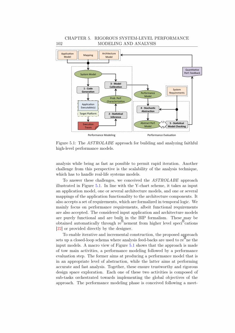
102CHAPTER 5. RIGOROUS SYSTEM-LEVEL PERFORMANCE
MODELING AND ANALYSIS
Applica'on Model
Mapping
1 -‐ Code Genera,on
2 -‐ Sta,s,cal Inference
Target Pla3orm
Applica'on Executable(s)
3 -‐ Model Calibra,on
5 -‐ Sta,s,cal Model Checking
Quan'ta've Perf. Feedback
System Requirements
Execu'on Traces
Architecture Model
4 -‐ Stochas,c Abstrac,on
Performance Modeling Performance Evalua'on
System Model
Prob. Perf. Characteriza'on
Performance Model
Abstract Perf. Model
Figure 5.1: The ASTROLABE approach for building and analyzing faithfulhigh-level performance models.
analysis while being as fast as possible to permit rapid iteration. Anotherchallenge from this perspective is the scalability of the analysis technique,which has to handle real-life systems models.
To answer these challenges, we conceived the ASTROLABE approachillustrated in Figure 5.1. In line with the Y-chart scheme, it takes as inputan application model, one or several architecture models, and one or severalmappings of the application functionality to the architecture components. Italso accepts a set of requirements, which are formalized in temporal logic. Wemainly focus on performance requirements, albeit functional requirementsare also accepted. The considered input application and architecture modelsare purely functional and are built in the BIP formalism. These may beobtained automatically through refinement from higher level specifications[22] or provided directly by the designer.
To enable iterative and incremental construction, the proposed approachsets up a closed-loop schema where analysis feed-backs are used to refine theinput models. A macro view of Figure 5.1 shows that the approach is madeof tow main activities, a performance modeling followed by a performanceevaluation step. The former aims at producing a performance model that isin an appropriate level of abstraction, while the latter aims at performingaccurate and fast analysis. Together, these ensure trustworthy and rigorousdesign space exploration. Each one of these two activities is composed ofsub-tasks orchestrated towards implementing the global objectives of theapproach. The performance modeling phase is conceived following a meet-

CHAPTER 5. RIGOROUS SYSTEM-LEVEL PERFORMANCEMODELING AND ANALYSIS 103
in-the-middle scheme to ensure the targeted abstraction trade-off, whereasthe analysis part is top-down as explained hereafter.
A Meet-in-the-Middle Modeling Solution
Top-Down Trajectory. The top-down branch of the modeling phase con-sists of generating a distributed implementation of the application and anassociated deployment strategy on the target architecture with respect tothe input mapping. This take advantage of the component-based modelingformalism we are adopting. This task is twofold, first a functional systemsmodel consisting of the combination of the application with the architecturewith respect to the given mapping is automatically built [44]. Then, auto-matic code generation is performed to produce a concrete implementation ofthe application functionality and the corresponding deployment schema withrespect to the mapping on the target platform given some runtime support.The target platform could be, depending on the design phase, an alreadyexisting board, a virtual prototype, or an Instruction-Set Simulator (ISS).The code generation step produces instrumented code with respect to theinput requirements. This specifies the performance dimension to estimate.
Bottom-Up Trajectory. The bottom-up branch of the modeling phase isperformed on the traces obtained by execution of generated code on thetarget platform. This consists of first learning a probabilistic characterizationof the specified performance aspects. As we will explain later in detail, thisrelies on a statistical inference procedure. This choice is made to captureperformance variability in a probabilistic manner. The second step in thisbottom-up part is the calibration of functional system models. This willaugment the BIP system model with performance information.
The meet-in-the-middle solution for performance modeling produces SBIPmodels encompassing functional behavior and performance details. We claimthat such an approach produces models with a good level of abstraction,which are sufficiently faithful for the earliest phases of the design.
A Formal Analysis Approach
In the ASTROLABE approach, we propose to use formal verificationas means to quantitatively analyze the obtained model with respect to theinput requirements. This is enabled because of the formal semantics of theSBIP formalism. We rely on statistical model checking since it combinessimulation and statistical techniques and thus provides a good trade-off be-tween speed and accuracy. For scalability issues, we will use our stochasticabstraction technique proposed in Chapter 4 to compute smaller models forfaster analysis.
The remainder of the chapter describes the different steps of performance
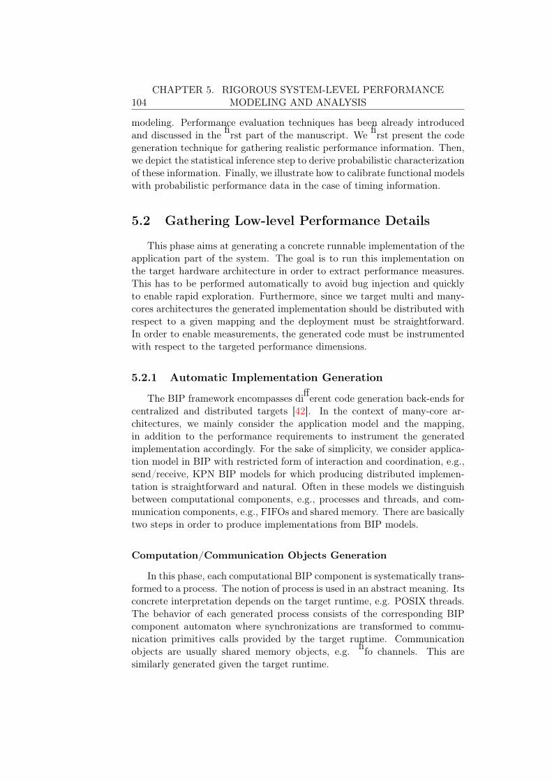
104CHAPTER 5. RIGOROUS SYSTEM-LEVEL PERFORMANCE
MODELING AND ANALYSIS
modeling. Performance evaluation techniques has been already introducedand discussed in the first part of the manuscript. We first present the codegeneration technique for gathering realistic performance information. Then,we depict the statistical inference step to derive probabilistic characterizationof these information. Finally, we illustrate how to calibrate functional modelswith probabilistic performance data in the case of timing information.
5.2 Gathering Low-level Performance Details
This phase aims at generating a concrete runnable implementation of theapplication part of the system. The goal is to run this implementation onthe target hardware architecture in order to extract performance measures.This has to be performed automatically to avoid bug injection and quicklyto enable rapid exploration. Furthermore, since we target multi and many-cores architectures the generated implementation should be distributed withrespect to a given mapping and the deployment must be straightforward.In order to enable measurements, the generated code must be instrumentedwith respect to the targeted performance dimensions.
5.2.1 Automatic Implementation Generation
The BIP framework encompasses different code generation back-ends forcentralized and distributed targets [42]. In the context of many-core ar-chitectures, we mainly consider the application model and the mapping,in addition to the performance requirements to instrument the generatedimplementation accordingly. For the sake of simplicity, we consider applica-tion model in BIP with restricted form of interaction and coordination, e.g.,send/receive, KPN BIP models for which producing distributed implemen-tation is straightforward and natural. Often in these models we distinguishbetween computational components, e.g., processes and threads, and com-munication components, e.g., FIFOs and shared memory. There are basicallytwo steps in order to produce implementations from BIP models.
Computation/Communication Objects Generation
In this phase, each computational BIP component is systematically trans-formed to a process. The notion of process is used in an abstract meaning. Itsconcrete interpretation depends on the target runtime, e.g. POSIX threads.The behavior of each generated process consists of the corresponding BIPcomponent automaton where synchronizations are transformed to commu-nication primitives calls provided by the target runtime. Communicationobjects are usually shared memory objects, e.g. fifo channels. This aresimilarly generated given the target runtime.

CHAPTER 5. RIGOROUS SYSTEM-LEVEL PERFORMANCEMODELING AND ANALYSIS 105
Deployment/Glue Code Generation
This produces code that maps the generated objects on the target hard-ware architecture. That is, the processes to specific processing units and thecommunication objects to memory.
Remark that the above process is strongly related to the target runtimeand that we only provide a generic description of the main steps. Additionaldetails are presented in Chapter 8 where we consider STHORM [155] as atarget architecture and an implementation of the MCAPI 1 standard as theunderlying runtime.
5.2.2 Instrumentation
Instrumentation consists of annotating the generated implementationwith specific function calls for measuring performance, e.g., timing, tem-perature. At this level, both communication and computation functionalityare handled similarly. Each communication routine or computation function-ality is enclosed withing specific annotations that specify the desired segmentto measure its time or energy consumption for instance. This is currentlydone manually and depend on the provided support of the target runtime.
5.3 Characterizing Performance Information
Depending on the observed performance dimension, collected data mayreflect timing behavior of computation or communication, temperature dis-sipation, energy consumption, or memory utilization. These performanceaspects are necessary together with functional behavior to enable trustwor-thy system analysis. Our goal is to characterize these details in order toobtain a faithful and abstract representation of performance data.
An important characteristic that must be considered is variability. Per-formance behavior is ideally deterministic, although due to several reasons,it is affected by some fluctuation which should be taken into considerationfor trustworthy analysis. Variable workloads are among these reasons, al-beit, there exist systems which have constant performance with respect tovariable inputs. Another source of fluctuation is the environment where thesystem will be deployed. For example, when considering temperature as aperformance metric, the role of the environment is preponderant since itdirectly impacts components temperature. Furthermore, some mechanismssuch as caches and arbitration impact performance evolution.
In general, variability induced by the above reasons may be determisti-cally characterized. However, besides being in contradiction with the system-level design guidelines, this is generally unfeasible. Precisely characterizingthe environment is unfeasible unless the system is designed for very specific
1. www.multicore-association.org/workgroup/mcapi.php

106CHAPTER 5. RIGOROUS SYSTEM-LEVEL PERFORMANCE
MODELING AND ANALYSIS
missions and targeted to a well known and controlled environment. Similararguments apply for the input data. Moreover, this requires to have detailedspecifications, which are rarely available in early design phases. Assumingthat such details are available, this will induce a considerable understandingand interpretation efforts, and consequently huge models. This eventuallyleads to an ad hoc approach which is tedious and error prone. We recall thatthe goal is to build faithful high-level models. Abstraction of details is thus amust. For instance, low-level arbitration and conflict resolution mechanismscannot be modeled in details during early design phases.
Our proposal is to consider that performance evolves probabilistically.We argue that this approach provides very natural abstractions. Let us con-sider a coin tossing experiment. In such a setting, it is common to considerthat the coin have a probabilistic outcome. However, this is an abstract viewof reality. Actually, if we are able to precisely characterize the coin, e.g., itsweight, the environment where the experiment is happening, e.g., wind speedand direction, and the flipping power, we would be able to precisely computethe outcome of the experiment using physics laws. Probabilistic modeling isa natural choice to abstract details either because we don’t care about themat the moment, or because we are not able to handle all of them, e.g., wedon’t have access to details, it takes too much time, they are too complex.
...
Shared Memory
Arbitration
f1 f2 fn
Figure 5.2: Memory access and arbitration mechanism.
Let us consider a situation where the goal is to characterize the executiontime of a function (or a process) f running periodically on a specific pro-cessing unit. The latter is assumed to execute only f , that is, no scheduling(context swap) overhead is induced. However, data to be processed by f isstored in a shared memory which is accessible by different processing unitsexecuting similar functions as shown in Figure 5.2. Thus, the execution timeof f will vary depending on the number of processes and the way they areaccessing the shared memory each time. Formally, if at time t, f tries toaccess the memory alone, the execution time will be x1. If P is the peri-odicity of f , and at time t + P f accesses the memory with y concurrentprocesses (in competition), the execution time will be x2 = x1 + �, where� is an arbitration overhead which depends on the number of processes y.Figure 5.3 below illustrates this setting.

CHAPTER 5. RIGOROUS SYSTEM-LEVEL PERFORMANCEMODELING AND ANALYSIS 107
begint t+P
execution
end
Coccurrent Memory AccessSimple Memory Access
memory access
Time
end
execution
x1
x2
Figure 5.3: Impact of arbitration mechanism on execution time.
Characterizing such behaviors probabilistically avoids modeling arbitra-tion mechanisms precisely and enables capturing the context in which theconsidered function is evolving, denoted interference, faithfully and in an ab-stract fashion. Again, it is possible to build a detailed model of interference,where the execution time evolves with respect to the number of processesaccessing the shared memory and given the used arbitration mechanism butthis is not our objective. This maybe need for refining the abstract model.
Probabilistic modeling provides various abstraction possibilities, rangingfrom simple point estimate, e.g., mean, variance, to more sophisticated mod-els, e.g., probability density function, stochastic processes. This depends onthe level of details required to resolve a given problem but also on the usedmethod to build such models. In our case, we aim to summarize performancedetails obtained from concrete executions while being faithful. Such proce-dure may be seen as learning general characteristic of some process, assumedto be probabilistic, by only observing some of its manifestations, e.g, runningdata. This bottom up approach, in contrast to building probabilistic modelsfrom specifications, is often called Statistical Inference.
We use Distribution Fitting, which will be detailed in Chapter 6, togetherwith and overview of statistical inference, to probabilistically characterizeperformance information. In distribution fitting, we consider probabilitydistributions as potential model for the data, i.e, it is only possible to char-acterize the data as a probability distribution. It is based on the threefollowing steps detailed in Chapter 6:
1. Exploratory Analysis: in this first step, we explore the data in term ofits shape to get a first idea on possible standard probability distribu-tions that may match.
2. Parameters Estimation: once we have some candidate distributions,we estimate their parameters using known estimation techniques.
3. Evaluation: finally, we evaluate the obtained fits using established sta-tistical tests.

108CHAPTER 5. RIGOROUS SYSTEM-LEVEL PERFORMANCE
MODELING AND ANALYSIS
5.4 Calibrating Functional Models
The calibration process aims to augment functional BIP models withperformance information, learned using distribution fitting. This transfor-mation produces stochastic BIP models that enables probabilistic analysis.The inferred probabilistic characterizations are used as probability distribu-tions related to the SBIP probabilistic variables that are added to model thedesired performance dimensions.
We focus on calibration of functional application models. The reasonfor this choice is to avoid building architecture components in the very earlydesign phases. Moreover, we are positioning this work in the setting where weare given a target architecture as part the system specifications. The mainquestion is thus how to map the different application functionalities intothe target architecture. However, we claim that the proposed approach canbe easily extended to handle architecture models as well. A previous workin the context embedded systems design in BIP [44] proposed a library ofarchitecture components. We can rely on this work to calibrate architecturecomponents in a similar manner.
5.4.1 Timing Information
Functional models are generally untimed or limited to functional use oftime, e.g., timeouts specification. They only concern the functional behaviorof the system. Calibrating such models with timing information has twomain consequences. First, it produces a timed model out of a “zero-time” oruntimed functional model. Second, since the timing information is proba-bilistically characterized, this will engender a stochastic model. The result isthus a new model, denoted performance model, that encompasses in one handthe functional behavior of the system and in the other hand the stochasticcharacterization of timing behavior.
Timing information may be of two types, Computation time or Commu-nication time. The first is the result of executing some application func-tionality on certain architecture component. Application functionality maybe a software process running on a programmable processing unit or de-signed as dedicated hardware component. Communication time is inducedby software or hardware components that solicit communication resourcessuch buses, NoCs, etc. These are handled differently when calibrating func-tional models.
In order to introduce computation time of a specific function within acomponent, a probabilistic variable related to the corresponding learned dis-tribution is first added then the learned computation time behavior is in-jected trough a waiting time using a tick interaction. Communication timeare slightly more complicated since are decomposed into begin and end ac-tions as shown in the remainder of this section.
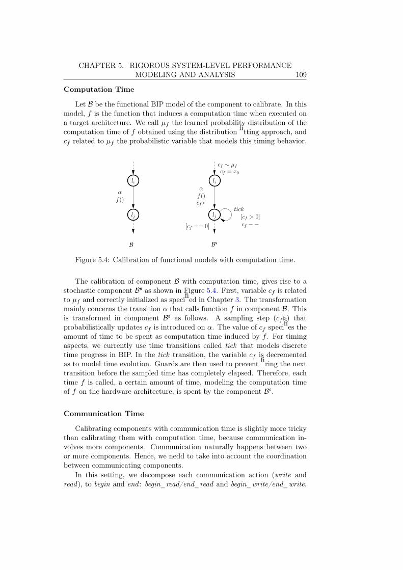
CHAPTER 5. RIGOROUS SYSTEM-LEVEL PERFORMANCEMODELING AND ANALYSIS 109
Computation Time
Let B be the functional BIP model of the component to calibrate. In thismodel, f is the function that induces a computation time when executed ona target architecture. We call µf the learned probability distribution of thecomputation time of f obtained using the distribution fitting approach, andcf related to µf the probabilistic variable that models this timing behavior.
li
lj
α
f()
li
lj
α
f()
[cf == 0]
tick
[cf > 0]
cf −−
B Bs
cf�
cf ∼ µf
cf = x0
Figure 5.4: Calibration of functional models with computation time.
The calibration of component B with computation time, gives rise to astochastic component Bs as shown in Figure 5.4. First, variable cf is relatedto µf and correctly initialized as specified in Chapter 3. The transformationmainly concerns the transition α that calls function f in component B. Thisis transformed in component Bs as follows. A sampling step (cf�) thatprobabilistically updates cf is introduced on α. The value of cf specifies theamount of time to be spent as computation time induced by f . For timingaspects, we currently use time transitions called tick that models discretetime progress in BIP. In the tick transition, the variable cf is decrementedas to model time evolution. Guards are then used to prevent firing the nexttransition before the sampled time has completely elapsed. Therefore, eachtime f is called, a certain amount of time, modeling the computation timeof f on the hardware architecture, is spent by the component Bs.
Communication Time
Calibrating components with communication time is slightly more trickythan calibrating them with computation time, because communication in-volves more components. Communication naturally happens between twoor more components. Hence, we nedd to take into account the coordinationbetween communicating components.
In this setting, we decompose each communication action (write andread), to begin and end : begin_read/end_read and begin_write/end_write.
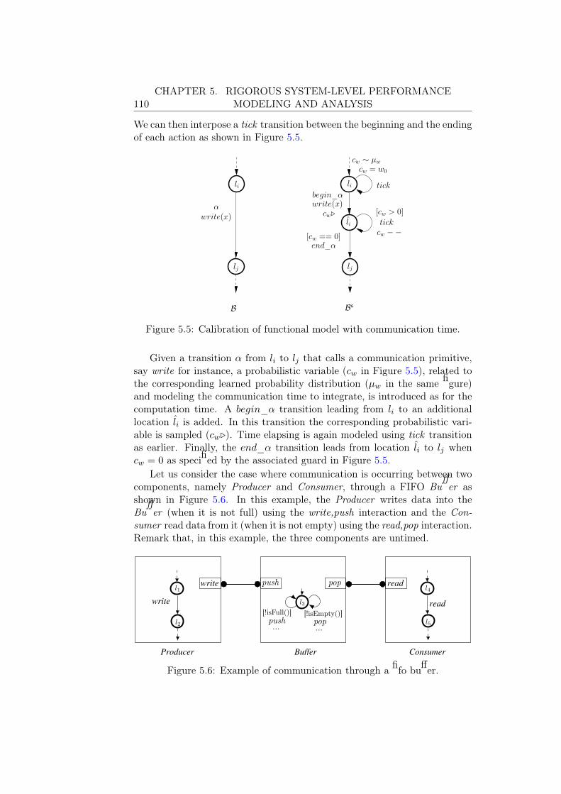
110CHAPTER 5. RIGOROUS SYSTEM-LEVEL PERFORMANCE
MODELING AND ANALYSIS
We can then interpose a tick transition between the beginning and the endingof each action as shown in Figure 5.5.
lj
B Bs
αwrite(x)
[cw == 0]end_α
cw −−
li li
l̂i
lj
[cw > 0]cw�write(x)begin_α
tick
tick
cw ∼ µw
cw = w0
Figure 5.5: Calibration of functional model with communication time.
Given a transition α from li to lj that calls a communication primitive,say write for instance, a probabilistic variable (cw in Figure 5.5), related tothe corresponding learned probability distribution (µw in the same figure)and modeling the communication time to integrate, is introduced as for thecomputation time. A begin_α transition leading from li to an additionallocation l̂i is added. In this transition the corresponding probabilistic vari-able is sampled (cw�). Time elapsing is again modeled using tick transitionas earlier. Finally, the end_α transition leads from location l̂i to lj whencw = 0 as specified by the associated guard in Figure 5.5.
Let us consider the case where communication is occurring between twocomponents, namely Producer and Consumer, through a FIFO Buffer asshown in Figure 5.6. In this example, the Producer writes data into theBuffer (when it is not full) using the write,push interaction and the Con-sumer read data from it (when it is not empty) using the read,pop interaction.Remark that, in this example, the three components are untimed.
write
write read
read
Producer Buffer Consumer
l4l1
l3
push pop
l2 l5
[!isFull()]push...
[!isEmpty()]pop...
Figure 5.6: Example of communication through a fifo buffer.

CHAPTER 5. RIGOROUS SYSTEM-LEVEL PERFORMANCEMODELING AND ANALYSIS 111
Given two probability distributions corresponding to the writing andreading time into/from the buffer, we will calibrate this model to intro-duce communication timing aspects. We will only calibrate the Producerand Consumer components and keep the Buffer untimed. This is Becausewe generally learn the communication time from the initiating processes per-spective (in this case Producer and Consumer). In such a setting, applyingthe transformation illustrated in Figure 5.5, requires to modify the push andpop actions of the Buffer as follows, begin_push, end_push, and begin_pop,end_pop. It is then straightforward to see that begin actions (respectivelyend actions) are synchronized together for all components as illustrated inFigure 5.7, which show the obtained model after calibration.
end_pop
...
end_push
Producer
end_pop
bgn_pop
end_rdtick3
bgn_rd
end_push
ConsumerBuffer
tick3
tick
tick1
bgn_wrt
end_wrt
tick1
bgn_wrt
tick1
end_wrt
...
bgn_push
... ...
bgn_rd
tick3
end_rd...
...
bgn_push
[!isFull()]
[!isEmpty()]bgn_pop
l3
l6
l7
l̂6
l5
l4l1
l̂1
l2
Figure 5.7: Calibration of the functional model in Figure 5.6.
The obtained execution sequence when applying the transformation illus-trated in Figure 5.5 is the following. When the Producer wants to send somedata, the interaction begin_write,begin_push is executed. This is only pos-sible when the Buffer have sufficient free memory. Otherwise, the Produceris blocked (tick1 transition in l1 is executed until some memory is freed).When begin_write,begin_push is executed, the corresponding probabilisticvariable is sampled and the tick1 transition in l̂1 becomes enabled. Duringthis time, the Consumer is blocked until writing has completed. The tick3transition on l6 enables correct time progress through the tick interaction.Omitting this transition engenders a deadlock (same as tick1 transition inl1). The sampled time elapses in l̂1 through the tick interaction. When itis done, the end_write,end_push is performed, which enables the Consumerto read following the same scheme. That is, begin_read,begin_pop, tick, thenend_read,end_pop. A complete typical execution sequence is thus 2
begin_write, begin_push → tickm → end_write, end_push →
begin_read, begin_pop → tickm → end_read, end_pop.
2. The used notations are as follow. action1, action2 depict an interaction, that is thestrong synchronization of the involved actions (see Chapter 3 for more details). The →stand for a sequence of actions. Finally, tickm means that the action is performed m time.

112CHAPTER 5. RIGOROUS SYSTEM-LEVEL PERFORMANCE
MODELING AND ANALYSIS
Remark 5.1 (Read/Write Blocking Time). It is important to remark fromthis example that the blocking time when reading or writing data is alreadycaptured by the functional part of the model. The push (respectively the pop)action of the Buffer component is blocking if the buffer is full (respectivelyempty). We have to take this into account when learning communicationtime distributions in order to correctly model it. To avoid modeling blockingtime redundantly, we have to learn only the communication time that doesnot include blocking parts. Such observation is quite important and enablesto precisely instrument the pertinent parts of the generated code to observeright timing aspects.
Observe that for the communication time, we didn’t used the same cal-ibration technique as for the computation time, that is, independently cali-brating components. The latter approach will not actually work correctly inthe case of communication as shown below.
Following the computation time calibration approach, illustrated in Fig-ure 5.4, will consist to calibrate the Producer by the time to write to thebuffer and the Consumer by the time to read from the buffer as shown inFigure 5.8. What is expected is that the producer performs the write action,then a certain time modeling the communication elapses before the consumercan perform read from the buffer. Then, some time modeling the readingfrom the buffer will elapse. That is,
write, push → tickm → read, pop → tickm
write read
Producer Buffer Consumer
write
tick1
read
tick1
tick1
tick3
tick3
tick3
tick
l3
push pop
[!isFull()]push...
[!isEmpty()]pop...
l1
l2
cw�
[cw > 0]
cw −−
l4
l5[cr > 0]
cr −−
cr�
[cr == 0][cw == 0]
cw ∼ µwcw = w0
cr ∼ µr
cr = r0
Figure 5.8: Bad calibration of the functional model in Figure 5.6.
However, if we transform the Producer and the Consumer as in Fig-ure 5.4, what will happen when running the system is the following. Whenthe Producer wants to send some data, the interaction write, push is per-formed (when the buffer is full or empty, the same reasoning as previously isapplied). As a consequence, in the Producer component, the tick1 transition

CHAPTER 5. RIGOROUS SYSTEM-LEVEL PERFORMANCEMODELING AND ANALYSIS 113
in l2 becomes enabled. Similarly, the pop action in the Buffer component be-comes enabled since the push action is performed instantaneously. We recallthat this component is kept untimed. The Consumer component is thus en-abled to read data. The interaction read, pop is assumed to become enabledwhenever pop is enabled. As specified in Chapter 3, the interaction involvingtick transitions is often given the lowest priority to enable system progressdeterministically. Hence, the interaction read, pop has a higher priority andis thus performed. The obtained execution sequence is thus
write, push → read, pop → tickm.
This sequence implies that the communication time (or at least a partof it) induced by writing data and the one induced by reading data (or atleast a part of it) are spent in parallel, which is not the desired behavior.Thus, the previous approach is not appropriate to calibrate components withcommunication time.
To correctly represent time in BIP, all the timed components, having ticktransitions, have to be correctly synchronized to enable overall time progress.A bit of care is needed to build such representations since bad synchroniza-tion of timed components lead inevitably to deadlocks as discussed for thel6 location in the previous example. It is possible to rely on the real-timecapabilities of BIP [1] instead of discrete tick transitions to capture timeevolution. This enable using built-in clock variables and transition firingwith respect to specified deadlines instead of guards. It is worth to men-tion that we are learning continuous probability distributions, while the theSBIP semantics introduced in Chapter 3 assumes finite models, hence finitedata domains. We are thus performing a discretization step of the obtainedprobability distributions to match the SBIP semantics.
5.5 Conclusions
In this chapter we presented the ASTROLABE approach for rigorousperformance modeling and analysis for system-level design of embedded sys-tems. The proposed approach combines several activities which are organizedtogether to answers various design challenges. The latter have been identi-fied as general ones and to more specific to performance aspects, which is theprimary goal of this work. The approach consists of first building abstractand faithful performance models. These are then analyzed with respect toperformance requirements in order to obtain quantitative feed-backs whichare used to refine initial models.
Starting from purely functional models of application and architecture,the modeling step first generates a distributed implementation for a targethardware architecture. The generated implementation is instrumented with

114CHAPTER 5. RIGOROUS SYSTEM-LEVEL PERFORMANCE
MODELING AND ANALYSIS
respect to given requirements to report on performance metrics. Executiontraces obtained by running this implementation on the target platform arethen statistically analyzed to learn a probabilistic characterization of per-formance behavior. Finally, the latter are injected into functional modelsthrough a calibration step to obtain stochastic performance models encom-passing functional and performance behavior.
The analysis phase takes as input the stochastic performance model andthe formalized requirements and operates an abstraction step to reduce themodel size. This is followed by a statistical model checking step that checksif the considered model that represents a given design alternative verify thegiven performance requirements or the expected properties. The results arethen used to refine the initial models or to modify the input mapping.
The described process enables vertical evolution through models refine-ment but also horizontal exploration of different performance dimensions fora given configuration, that is, a specific mapping with a fixed set of pa-rameters, e.g., FIFOs sizes. In the above description we mainly focusedon timing. Other performance aspects such as energy or temperature, canbe similarly handled in the approach by introducing probabilistic variablesmodeling temperature evolution or energy consumption. This will constitutethe subject of future work and further discussions in the conclusion. Before,we detail in the next chapter the distribution fitting technique we use forprobabilistically characterizing performance information.

Chapter 6Statistical Characterization of
Performance
In the previous chapter, we presented the ASTROLABE approach andoverview its different steps. We briefly discussed how to statistically char-acterize performance information obtained from concrete executions. In thischapter, we present in more detail the general statistical inference procedureand introduce specifically distribution fitting, the method we use to learnprobability distributions that characterize low-level performance data.
6.1 Statistical Inference
Probabilistic modeling often consists of deriving probabilistic character-izations from specifications of an artifact. Another possible approach, inthis context, is when we are given data obtained from running the artifact(this may be for instance polling data, or data from a dice experiment). Inthis case, inferential analysis, that is bottom up trajectory must be taken tobuild probabilistic model. Statistical inference is thus the process of proba-bilistically characterizing the behavior of an artifact from data. In our case,data concern performance information obtained from concrete execution orlow-level simulation of functional models on a target hardware platform.
From this perspective, data is assumed to be generated by a stochas-tic process for which the governing law is unknown. Our goal is to infersuch a law from a subset of observations, called a sample, since the wholepopulation is generally not available. Formally, given x1, ..., xn a set of ob-servations, we assume that there exist X1, ..., Xn independent and identicallydistributed (iid) random variables such that xi is a possible realization of Xi.Independence is to be understood in the sense that one outcome of a randomexperiment does not affect the outcome of another. Identically distributedrandom variables basically means that they all follow the same probability
115

116CHAPTER 6. STATISTICAL CHARACTERIZATION OF
PERFORMANCE
distribution D(ω) where ω ∈ Θ is the set of parameters of the distributiondefined over the space Θ.
One should pay attention to the independence assumption above sincethis will enable accurate generalizations of the inference results. Note thatthe goal is not only to characterize the available data. The most importantis to be able to generalize the result to the generating process. That is,to conclude that the generating process follows some probability distribu-tion. Concretely, the independence assumption states that observations areobtained randomly. Two possible configurations are generally possible:
– The first is when an experiment is conceived with the aim to observe aspecific phenomenon. In such a case, independence is easy to guaranteesince the procedure is completely controlled.
– The second case is when we perform observations on a process whichis not under our control (or partially controlled), e.g simulation orexecution of a system.
We are in the latter setting, where independence cannot be assumed butmust be checked. Several ways exists to check independence albeit not alwayseasy to understand. One can, for example, use specific plots, e.g., Lag plot,which require expertise for interpretation or rely on existing statistical testssuch as Box-Pierce [47], Ljung-Box [151], and runs test 1.
Several inference approaches giving different abstractions are available.These learning procedures may be automatic or not and may produce variousprobabilistic models ranging from probability distributions to Markov ormore general stochastic models. In section 4.4, we detailed several automatictechniques based on machine learning that allow to learn such probabilisticmodels. These could be used in this context to characterize performanceinformation.
It is worth to mention that adopting a method or another, in additionto being dependent on the desired abstraction, also depends on the availabledata which reflect the artifact dynamics under certain circumstances. Datamay show a certain structure, that is, dependency on other factors. Forinstance, the execution time of a certain function may depend on its inputs,the communication delay may depend on the number of process that solicitthe communication media at that time, the temperature of a component ata time t depends on its temperature at time t − 1 but may also depend onthe temperature of others components or the ambient temperature. Thissuggest a state-based characterization of the data or an analytical formulathat capture this relationship. The latter are for instance obtained usingtime series methods such as regression analysis approaches [8, 96, 175, 3]that characterize data as a random variable called dependent obtained as alinear or non-linear relations of a set of other variables called independentand some random error, called noise.
1. http://www.itl.nist.gov/div898/handbook/eda/section3/eda35d.htm
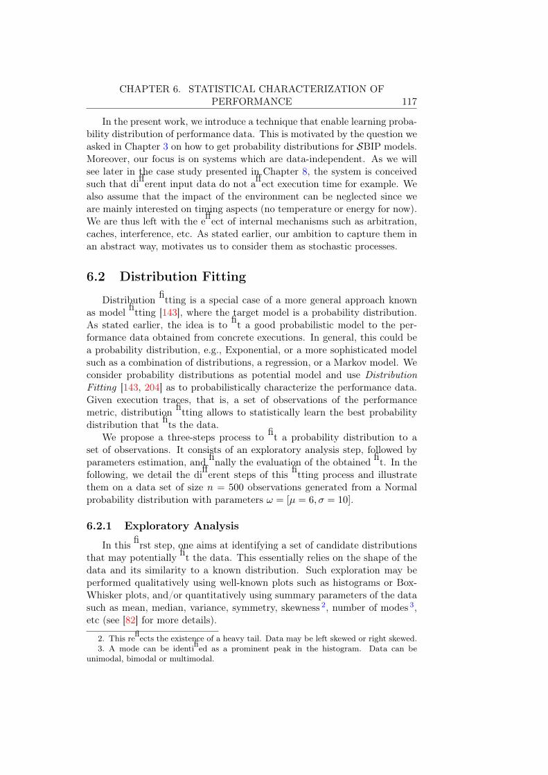
CHAPTER 6. STATISTICAL CHARACTERIZATION OFPERFORMANCE 117
In the present work, we introduce a technique that enable learning proba-bility distribution of performance data. This is motivated by the question weasked in Chapter 3 on how to get probability distributions for SBIP models.Moreover, our focus is on systems which are data-independent. As we willsee later in the case study presented in Chapter 8, the system is conceivedsuch that different input data do not affect execution time for example. Wealso assume that the impact of the environment can be neglected since weare mainly interested on timing aspects (no temperature or energy for now).We are thus left with the effect of internal mechanisms such as arbitration,caches, interference, etc. As stated earlier, our ambition to capture them inan abstract way, motivates us to consider them as stochastic processes.
6.2 Distribution Fitting
Distribution fitting is a special case of a more general approach knownas model fitting [143], where the target model is a probability distribution.As stated earlier, the idea is to fit a good probabilistic model to the per-formance data obtained from concrete executions. In general, this could bea probability distribution, e.g., Exponential, or a more sophisticated modelsuch as a combination of distributions, a regression, or a Markov model. Weconsider probability distributions as potential model and use DistributionFitting [143, 204] as to probabilistically characterize the performance data.Given execution traces, that is, a set of observations of the performancemetric, distribution fitting allows to statistically learn the best probabilitydistribution that fits the data.
We propose a three-steps process to fit a probability distribution to aset of observations. It consists of an exploratory analysis step, followed byparameters estimation, and finally the evaluation of the obtained fit. In thefollowing, we detail the different steps of this fitting process and illustratethem on a data set of size n = 500 observations generated from a Normalprobability distribution with parameters ω = [µ = 6,σ = 10].
6.2.1 Exploratory Analysis
In this first step, one aims at identifying a set of candidate distributionsthat may potentially fit the data. This essentially relies on the shape of thedata and its similarity to a known distribution. Such exploration may beperformed qualitatively using well-known plots such as histograms or Box-Whisker plots, and/or quantitatively using summary parameters of the datasuch as mean, median, variance, symmetry, skewness 2, number of modes 3,etc (see [82] for more details).
2. This reflects the existence of a heavy tail. Data may be left skewed or right skewed.3. A mode can be identified as a prominent peak in the histogram. Data can be
unimodal, bimodal or multimodal.
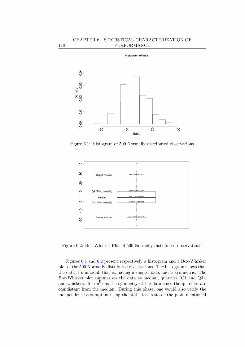
118CHAPTER 6. STATISTICAL CHARACTERIZATION OF
PERFORMANCE
Histogram of data
data
Density
-20 0 20 40
0.00
0.01
0.02
0.03
0.04
Figure 6.1: Histogram of 500 Normally distributed observations.
-20
-10
01
02
03
04
0
-17.1676641453136
-1.30676498597915
4.30730137645451
10.6652286027237
28.4290467955677
Lower whisker
Q1 (First quartile)
Median
Q3 (Third quartile)
Upper whisker
Figure 6.2: Box-Whisker Plot of 500 Normally distributed observations.
Figures 6.1 and 6.2 present respectively a histogram and a Box-Whiskerplot of the 500 Normally distributed observations. The histogram shows thatthe data is unimodal, that is, having a single mode, and is symmetric. TheBox-Whisker plot summarizes the data as median, quartiles (Q1 and Q3),and whiskers. It confirms the symmetry of the data since the quartiles areequidistant from the median. During this phase, one would also verify theindependence assumption using the statistical tests or the plots mentioned
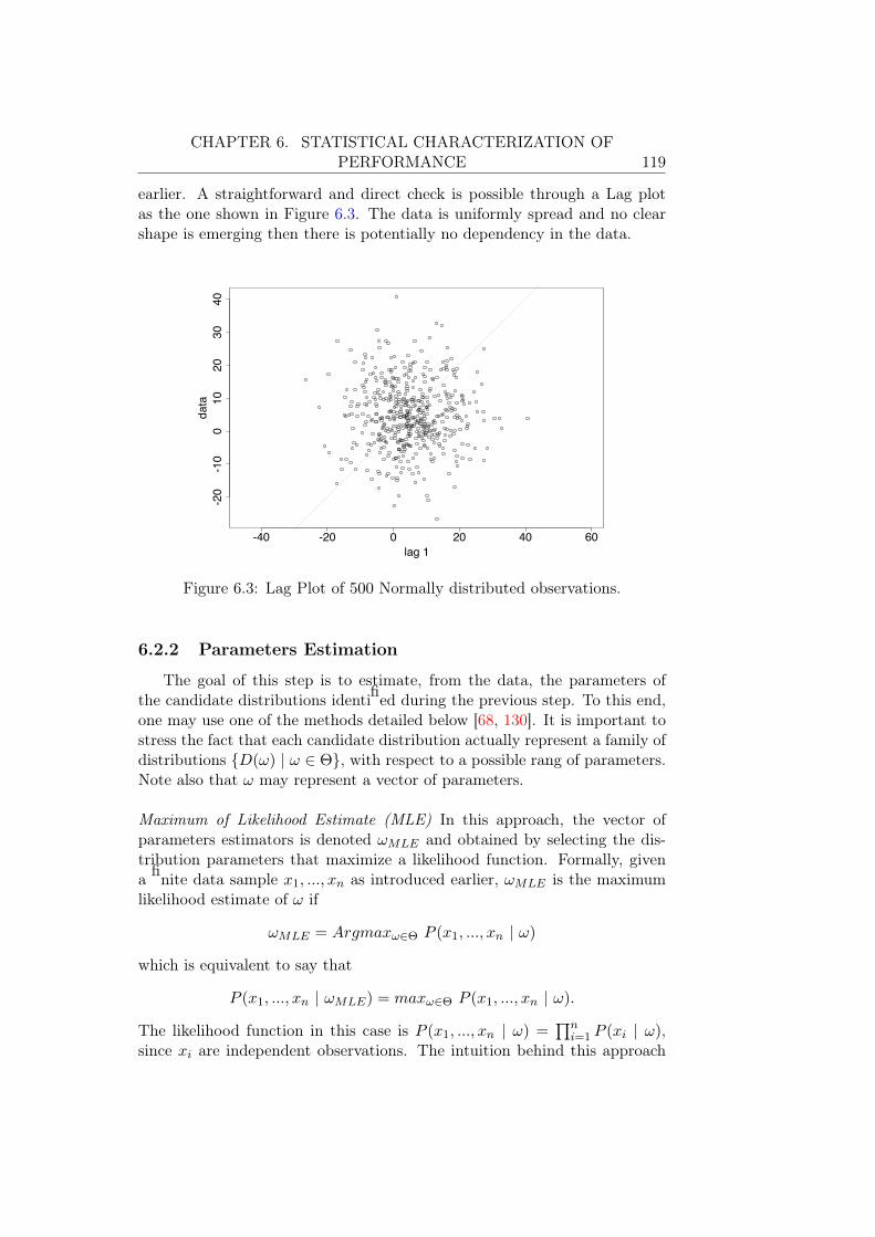
CHAPTER 6. STATISTICAL CHARACTERIZATION OFPERFORMANCE 119
earlier. A straightforward and direct check is possible through a Lag plotas the one shown in Figure 6.3. The data is uniformly spread and no clearshape is emerging then there is potentially no dependency in the data.
-40 -20 0 20 40 60
-20
-10
01
02
03
04
0
lag 1
da
ta
Figure 6.3: Lag Plot of 500 Normally distributed observations.
6.2.2 Parameters Estimation
The goal of this step is to estimate, from the data, the parameters ofthe candidate distributions identified during the previous step. To this end,one may use one of the methods detailed below [68, 130]. It is important tostress the fact that each candidate distribution actually represent a family ofdistributions {D(ω) | ω ∈ Θ}, with respect to a possible rang of parameters.Note also that ω may represent a vector of parameters.
Maximum of Likelihood Estimate (MLE) In this approach, the vector ofparameters estimators is denoted ωMLE and obtained by selecting the dis-tribution parameters that maximize a likelihood function. Formally, givena finite data sample x1, ..., xn as introduced earlier, ωMLE is the maximumlikelihood estimate of ω if
ωMLE = Argmaxω∈Θ P (x1, ..., xn | ω)
which is equivalent to say that
P (x1, ..., xn | ωMLE) = maxω∈Θ P (x1, ..., xn | ω).
The likelihood function in this case is P (x1, ..., xn | ω) =�n
i=1 P (xi | ω),since xi are independent observations. The intuition behind this approach

120CHAPTER 6. STATISTICAL CHARACTERIZATION OF
PERFORMANCE
is that the probability to obtain the observations xi when selecting the goodparameters ω is expected to be the highest, otherwise (when the selectedparameters are not good) it is low. It is worth to mention that MLE estimatesmight be not unique or even, in some cases, not exist.
For the considered 500 observations, using the MLE method we obtainωLME = [µMLE = 4.82,σMLE = 9.78]. We also report a standard error(SE) of the estimates: 0.44 for the mean and 0.31 for the standard devia-tion. This reflect the marge of error due to data fluctuation. When fixing aconfidence level of 95% for instance, we can provide a confidence interval forthe estimations [82]. For the mean for example, this interval is equal to 4
5.74± (1.96× 0.44) � [3.96, 5.68].
This meas that if we generate several data sets of size 500 from a Normaldistribution with µ = 6 and σ = 10, then 95% of these sets will have a meanestimator within this interval.
Moments Matching Estimate (MME) We denote the vector of parametersestimators as ωMME . In this approach, the idea is to resolve a system ofm independent linear equations. These are obtained with respect to thedifferent moments of the considered iid random variables Xi, where m isthe number of parameters of the underlying distributions. That is, it isrequired to have exactly 5 as many moments as the number of parametersof the distributions. In the case of the Normal distribution for instance,we have only two parameters (µ,σ). Then, we will have a linear systemcomposed of two equations to resolve. Concretely, the vector of estimatorsis ωMME = [µMME ,σMME ].
The moments m of a random variable following a certain probabilitydistribution corresponds to the expectation values E[Xm
i ] of that variable.For instance, for a Normal distribution, the first moment is simply the mean,i.e., E[Xi] = µ and the second moment is E[(Xi − µ)2] = σ2. Based on theweak law of large numbers [8], in the case of n = 500 normally distributedobservations, the system of equations is
µMME = 1n
�ni=1Xi
σ2MME = 1
n
�ni=1(Xi − µMME)
2
That is, we are simply estimating the mean of the population by the meanof the considered sample and similarly for the standard deviation. The es-timated values are ωMME = [µMME = 4.73,σMME = 9.17]. This approach
4. The general formula to compute a confidence interval (CI) for the mean, under theassumption that the data is drawn from a Normal distribution, is CI = PE± (1.96×SE)for a 95% confidence level and where PE is the point estimate obtained using MLE forinstance.
5. In generalized method of moments (GMM), we may have more equations than theparameters to estimate. This induce the existence of several possible solutions.
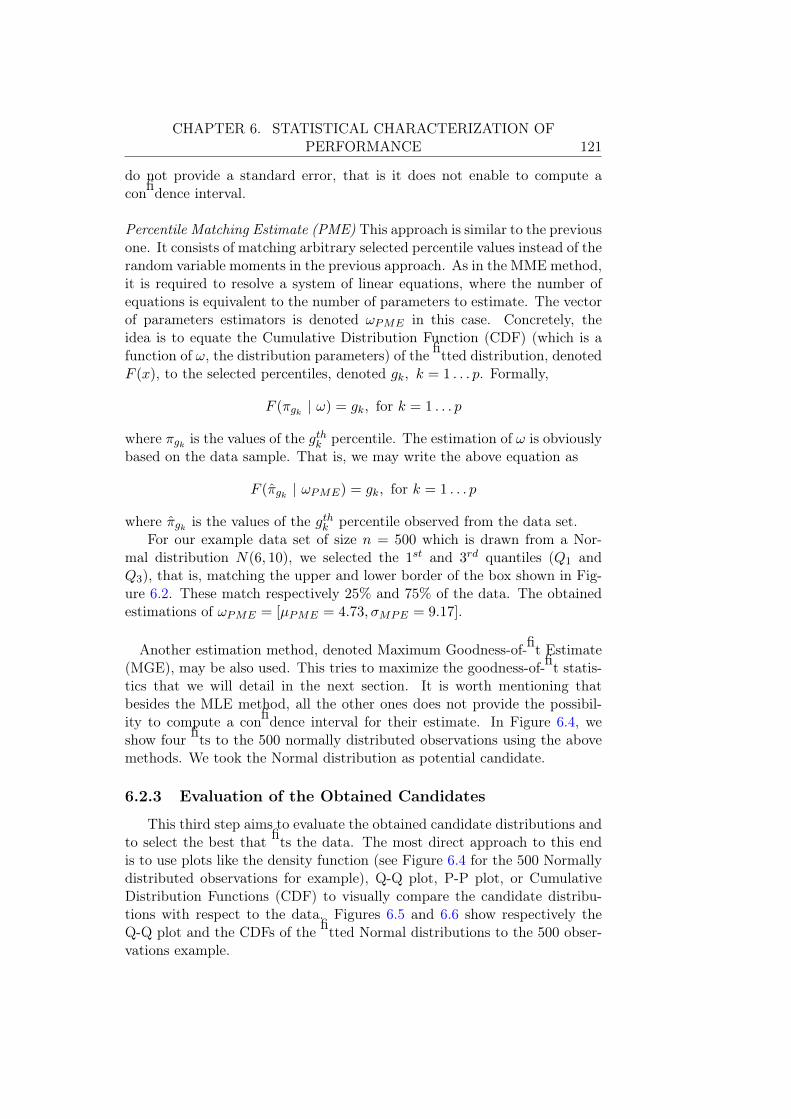
CHAPTER 6. STATISTICAL CHARACTERIZATION OFPERFORMANCE 121
do not provide a standard error, that is it does not enable to compute aconfidence interval.
Percentile Matching Estimate (PME) This approach is similar to the previousone. It consists of matching arbitrary selected percentile values instead of therandom variable moments in the previous approach. As in the MME method,it is required to resolve a system of linear equations, where the number ofequations is equivalent to the number of parameters to estimate. The vectorof parameters estimators is denoted ωPME in this case. Concretely, theidea is to equate the Cumulative Distribution Function (CDF) (which is afunction of ω, the distribution parameters) of the fitted distribution, denotedF (x), to the selected percentiles, denoted gk, k = 1 . . . p. Formally,
F (πgk | ω) = gk, for k = 1 . . . p
where πgk is the values of the gthk percentile. The estimation of ω is obviouslybased on the data sample. That is, we may write the above equation as
F (π̂gk | ωPME) = gk, for k = 1 . . . p
where π̂gk is the values of the gthk percentile observed from the data set.For our example data set of size n = 500 which is drawn from a Nor-
mal distribution N(6, 10), we selected the 1st and 3rd quantiles (Q1 andQ3), that is, matching the upper and lower border of the box shown in Fig-ure 6.2. These match respectively 25% and 75% of the data. The obtainedestimations of ωPME = [µPME = 4.73,σMPE = 9.17].
Another estimation method, denoted Maximum Goodness-of-fit Estimate(MGE), may be also used. This tries to maximize the goodness-of-fit statis-tics that we will detail in the next section. It is worth mentioning thatbesides the MLE method, all the other ones does not provide the possibil-ity to compute a confidence interval for their estimate. In Figure 6.4, weshow four fits to the 500 normally distributed observations using the abovemethods. We took the Normal distribution as potential candidate.
6.2.3 Evaluation of the Obtained Candidates
This third step aims to evaluate the obtained candidate distributions andto select the best that fits the data. The most direct approach to this endis to use plots like the density function (see Figure 6.4 for the 500 Normallydistributed observations for example), Q-Q plot, P-P plot, or CumulativeDistribution Functions (CDF) to visually compare the candidate distribu-tions with respect to the data. Figures 6.5 and 6.6 show respectively theQ-Q plot and the CDFs of the fitted Normal distributions to the 500 obser-vations example.
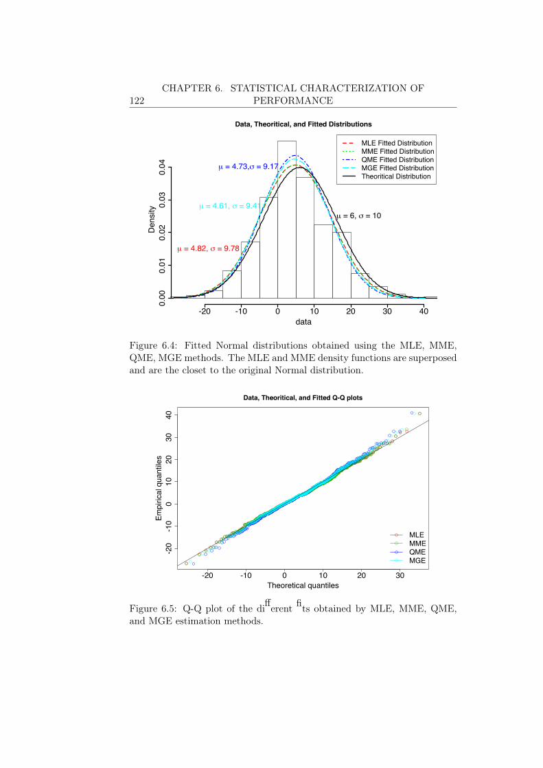
122CHAPTER 6. STATISTICAL CHARACTERIZATION OF
PERFORMANCE
Data, Theoritical, and Fitted Distributions
data
De
nsity
-20 -10 0 10 20 30 40
0.0
00
.01
0.0
20
.03
0.0
4
fit 1fit 2fit 3fit 4
μ = 6, σ = 10
μ = 4.82, σ = 9.78
μ = 4.73,σ = 9.17
μ = 4.61, σ = 9.41
MLE Fitted DistributionMME Fitted DistributionQME Fitted DistributionMGE Fitted DistributionTheoritical Distribution
Figure 6.4: Fitted Normal distributions obtained using the MLE, MME,QME, MGE methods. The MLE and MME density functions are superposedand are the closet to the original Normal distribution.
-20 -10 0 10 20 30
-20
-10
01
02
03
04
0
Data, Theoritical, and Fitted Q-Q plots
Theoretical quantiles
Em
pir
ica
l qu
an
tile
s
MLEMMEQMEMGE
Figure 6.5: Q-Q plot of the different fits obtained by MLE, MME, QME,and MGE estimation methods.

CHAPTER 6. STATISTICAL CHARACTERIZATION OFPERFORMANCE 123
-20 -10 0 10 20 30 40
0.0
0.2
0.4
0.6
0.8
1.0
Data, Theoritical, and Fitted CDFs
data
CD
F
fit 1fit 2fit 3fit 4
MLE Fitted CDFMME Fitted CDFQME Fitted CDFMGE Fitted CDFTheoritical CDF
Figure 6.6: Comparison of the Cumulative Distribution Functions (CDFs)of the Normal fits obtained by using MLE, MME, QME, GME on the 500Normally distributed observations.
Using plots requires human interpretation, which may be subjective andchange from a person to another. It is thus better to rely on numericalmeasures or scores that quantify how close or far a candidate fit is from thedata. This is usually performed using a goodness-of-fit test which is based onwell-known statistics especially designed for this task, such as Kolmogorov-Smirnov (K-S), Anderson-Darling (A-D), and Carmer-Von Mises (C-VM)[204, 130] in the case of continuous distributions, or on the χ2 test [68, 8]when the fitted distribution is discrete. We illustrate hereafter the main in-tuition of the statistics used in the continuous case since these are our target.
Goodness-of-fit test A goodness-of-fit test is a special case of a hypothesistest where the goal is to give a measure of how well the null hypothesis H0 iscompatible with the considered data, without using an alternative hypothesisH1 [68] (as was the case for example in Chapter 2). This may be performed byconstructing a test static whose value reflects the agreement degree betweenthe null hypothesis H0 and the data. In this case, the hypothesis H0 statesthat observed data is coming from a population governed by a candidatedistribution (obtained in the previous steps).
Let us consider again the coin tossing experiment. Assume one tossesthe coin N times and obtains h heads and t = N − h tails. Let us considerthe hypothesis H0 as “the coin is unbiased or fair ”, that is the probabilitiesfor heads and tails are equal. Our goal is to quantify to what extent the

124CHAPTER 6. STATISTICAL CHARACTERIZATION OF
PERFORMANCE
observed h and t for certain N are consistent with H0. In this case, one canfor instance use the number of heads h as a test statistics (h is a randomvariable). This is known to follow a binomial distribution, h ∼ B(N, p),where N is the number of tosses and p is the probability to obtain a headoutcome in each toss. When the coin is assumed to be fair, that is, H0 istrue, the probability p = 0.5. Given these, we can compute the probabilityto observe h heads in N tosses using the following formula
f(h,N, p) = P (h) = CNh ph(1− p)N−h. (6.1)
We take N = 20 tosses and we assume we observed h = 17 heads.Given N = 20 and p = 0.5, we know that the expected value for h isE[h] = Np = 10 (expectation of a Binomial random variable). We canobserve a clear difference between the expected value of number of heads forthis configuration and what we actually observed. In order to quantify thelevel of this discrepancy, one may give the probability to obtain such resultsor more extreme given the hypothesis H0 is true, that is,
P (to obtain the observed results or more extreme | H0 is true),
which is known as p-value [8]. In this case, the observed result is h = 17and more extreme results would be h = 18, 19, 20 but also h = 0, 1, 2, 3(symmetrical values). Using equation 6.1, and by summing the probabilitiesfor each h above, one obtain P = 0.0026. When specifying a significancelevel α, we may take a decision with respect to hypothesis H0 as follow.
– If the p-value is lower than α, we conclude that it is very unlikely toget the observed data when the null hypothesis were actually true, andhence we reject H0.
– If the p-value is greater than α, we conclude that it is likely to get theobserved data even if the null hypothesis were true, and hence we donot reject H0.
In general, we specify α = 0.05 or 0.01. In this example, for both α, thehypothesis H0 is rejected since 0.0026 < 0.01. That is, given the observationsof 17 heads in 20 tosses, we reject the hypothesis that the used coin is fair.
The test statistics presented above were specifically designed to test ifa given sample was drawn from a certain distribution. They use differentconstructions for testing such hypothesis. For instance, the Kolmogorov-Smirnov [130] statistic is based on the measure of the difference between thetheoretical and the empirical cumulative distribution function. Similarly theAnderson-Darling [130] and the Carmer-Von Mises [204] statistics are basedon difference measure of the cumulative distributions function. However,they perform weighted and quadratic tests. The For example, the Anderson-Darling statistic gives more weight to the information on the tail.
For the 500 normally distributed observations, the obtained evaluationresults using the above methods are presented in Table 6.1. We observe

CHAPTER 6. STATISTICAL CHARACTERIZATION OFPERFORMANCE 125
that the K-S statistic is lower than the significance level α = 0.05 fixed inthis case, and suggests to reject the Normal fit, while both A-D and C-VMare greater. We thus accept the hypothesis that the data is drawn from aNormal process.
Kolmogorov-Smirnov Carmer-Von Mises Anderson-Darling
MLE 0.0355 0.1090 0.5778
MME 0.0355 0.1090 0.5778
QME 0.0331 0.0852 0.8180
MGE 0.0295 0.0678 0.5954
Table 6.1: Results of the goodness-of-fit tests of the fitted distributions ob-tained using the previous estimation methods on the 500 considered obser-vations with a significance level α = 0.05.
The last phase of the distribution fitting process is quite important sinceit allows to select the best distribution that fits the data. In addition tothe aforementioned test statistics, other tools may be of use, like BayesianInformation Criterion (BIC) and Akaike Information Criterion (AIC) [130]which provide a way to quantitatively compare the candidate models basedon the likelihood function and the number of parameters used in the model.The latter is mainly aimed to prevent over fitting issues, that is, to choosea model (in our case a distribution) with an important number of param-eters. For instance, for the 500 Normally distributed observations, we areconsidering the AIC and BIC scores are shown in Table 6.2 below.
BIC score AIC score
MLE 3713.4 3705.0
MME 3713.4 3705.0
QME 3718.1 3709.6
MGE 3715.3 3706.9
Table 6.2: BIC and AIC scores for the four previously illustrated parametersestimation methods on the 500 normally distributed observations.
By crossing the quantitative results with the obtained plots, it is clearthat the Normal distribution is a good fit for the data (which is expectedin this example, because we initially generated these observations using aNormal distribution). Moreover, we may use the estimation obtained by theMLE and MME methods since they are the closest to the original parameters.In the general case, where the original parameters are unknown, we choosethe fit which is accepted by a maximum number of tests, having great p-values, and lower BIC/AIC scores.

126CHAPTER 6. STATISTICAL CHARACTERIZATION OF
PERFORMANCE
It is important to mention that in some cases, a pre-processing phase ofthe data may be required before performing the fitting. For instance, datamay need scaling, outliers analysis (we will give an example about outliersin the next chapter), and/or log transformations. Such requirements areusually detected during the exploratory analysis phase.
6.3 Conclusions
In this chapter, we presented the general statistical inference setting andintroduced a distribution fitting process in order to characterize performanceinformation in a probabilistic fashion. The proposed process is composedof three steps potentially leading to a probability distribution that fits theinput data. We recall that for distribution fitting to work properly, it isrequired that the data do not show any dependency. This assumption mustbe checked during the first exploratory analysis step, which also enables toidentify candidate distributions that characterize the data. The second stepin the process is to estimate the parameters of the identified distributions.Finally, an evaluation step of the obtained distributions and estimated pa-rameters is performed.
In the next chapter, we will present a tool that assists designers to ac-complish this process, as part of a complete tool-flow covering most of thesteps of the ASTROLABE approach.
Chapter 7The ASTROLABE Tool-flow
In the previous chapters of this part, we presented ASTROLABE, a rig-orous method for performance modeling and evaluation for early phases ofsystem-level design. We mainly depicted the approach philosophy and itsdifferent steps, that is, code generation and instrumentation together withstatistical inference and model calibration for building faithful performancemodels, followed by stochastic abstraction and statistical model checking forperformance evaluation.
Design automation has become essential for modern companies to beproactive and to be able to bring quick answers to rapidly evolving markets.Besides time reduction, automation reduces manual tasks which are errorprone and hence reduces debugging and testing efforts and tends to increasedesigner efficiency. The ASTROLABE approach is in line with this viewin that it is conceived to enable a maximum of automation. This chapterdescribes a tool-flow set-up to automate and materialize the proposed ap-proach. The flow is composed of several interconnected tools that automatemost of the approach tasks, that is:
– Automatic generation of distributed implementations,– Assisting designer to perform distribution fitting,– Automatically learning stochastic abstraction for faster analysis,– Statistical model checking the obtained models with respect to perfor-
mance requirements.
Model instrumentation and calibration are still performed manually at thecurrent state.
7.1 Overview
The tool-flow is centered on the BIP and the SBIP models. All themanipulated models are either BIP models or stochastic ones expressed inSBIP. Figure 7.1 shows the different tools used in the different phases of
127
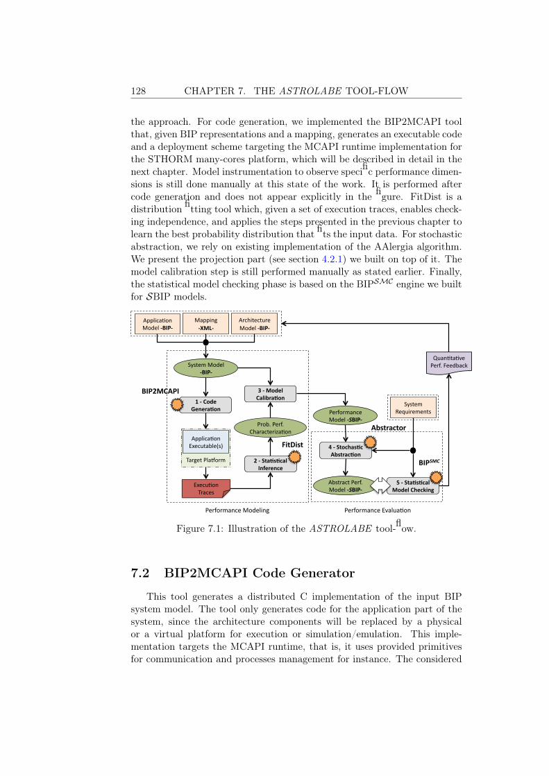
128 CHAPTER 7. THE ASTROLABE TOOL-FLOW
the approach. For code generation, we implemented the BIP2MCAPI toolthat, given BIP representations and a mapping, generates an executable codeand a deployment scheme targeting the MCAPI runtime implementation forthe STHORM many-cores platform, which will be described in detail in thenext chapter. Model instrumentation to observe specific performance dimen-sions is still done manually at this state of the work. It is performed aftercode generation and does not appear explicitly in the figure. FitDist is adistribution fitting tool which, given a set of execution traces, enables check-ing independence, and applies the steps presented in the previous chapter tolearn the best probability distribution that fits the input data. For stochasticabstraction, we rely on existing implementation of the AAlergia algorithm.We present the projection part (see section 4.2.1) we built on top of it. Themodel calibration step is still performed manually as stated earlier. Finally,the statistical model checking phase is based on the BIPSMC engine we builtfor SBIP models.
Applica'on Model -‐BIP-‐
Mapping -‐XML-‐
1 -‐ Code Genera2on
2 -‐ Sta2s2cal Inference
Target Pla3orm
Applica'on Executable(s)
3 -‐ Model Calibra2on
5 -‐ Sta2s2cal Model Checking
Quan'ta've Perf. Feedback
System Requirements
Execu'on Traces
Architecture Model -‐BIP-‐
4 -‐ Stochas2c Abstrac2on
Performance Modeling Performance Evalua'on
System Model -‐BIP-‐
Prob. Perf. Characteriza'on
Performance Model -‐SBIP-‐
Abstract Perf. Model -‐SBIP-‐
BIP2MCAPI
FitDist
BIPSMC
Abstractor
Figure 7.1: Illustration of the ASTROLABE tool-flow.
7.2 BIP2MCAPI Code Generator
This tool generates a distributed C implementation of the input BIPsystem model. The tool only generates code for the application part of thesystem, since the architecture components will be replaced by a physicalor a virtual platform for execution or simulation/emulation. This imple-mentation targets the MCAPI runtime, that is, it uses provided primitivesfor communication and processes management for instance. The considered

CHAPTER 7. THE ASTROLABE TOOL-FLOW 129
MCAPI implementation is provided by CEA 1 in the context of the SMECYproject 2 and is specifically designed for the STHORM many-cores platform,which is designed by STMicroelectronics 3. Given the functional BIP model,a set of design parameters, e.g., buffers sizes, and a mapping, this step con-sists to generate the low-level running C/MCAPI code for STHORM plat-form. This is performed in two main steps: (1) Object generation, that isprocesses, queues, and shared objects, and (2) Deployment/Glue code gen-eration, which maps the generated objects on the target platform.
7.2.1 Process Generation
During this step, each BIP component is transformed to a C/MCAPIprocess. A challenging point at this level is to generate small set of processlocal variables to fit the small amount of available memory per process stackon STHORM. The generated processes are basically composed of two parts:
– Initialization: in this part, BIP components interfaces (ports) aretransformed into equivalent MCAPI endpoints. The generated processendpoints are initialized, opened, and connected to other processes inthis same block. Moreover, endpoints memory attributes are generatedto allocate FIFO buffers and shared objects (given their sizes) and tomap them into specific memory locations. MCAPI implementationfor STHORM provides several possibility to map buffers into specifictarget memory as shown in Table 7.1. Buffers could be mapped eitherin L3, L2 or L1 memory using the attributes shown in the table. ForL1 memory, it depends on the sender/receiver processes location. Ifthese run in the same cluster, the buffer is allocated in the L1 memoryof that cluster. Otherwise, it is mapped in the L1 of the cluster wherethe sender (respectively the receiver) runs.
Target Memory Sender Attribute Receiver Attribute
L3 Remote RemoteL2 Shared Shared
Receiver L1 Shared LocalSender L1 Local Shared
Table 7.1: MCAPI endpoints memory attributes.
– Behavior: in this part, BIP component behavior is transformed toequivalent C code with MCAPI primitives calls. It consists essentiallyon an infinite while loop with several steps (using Switch/Case state-ments) reproducing the BIP automata behavior. In the generated code,
1. Commisariat à l’energie atomique et aux energies alternatives, http://www.cea.fr2. http://www.artemis-ia.eu/project/25-smecy.html
3. http://www.st.com
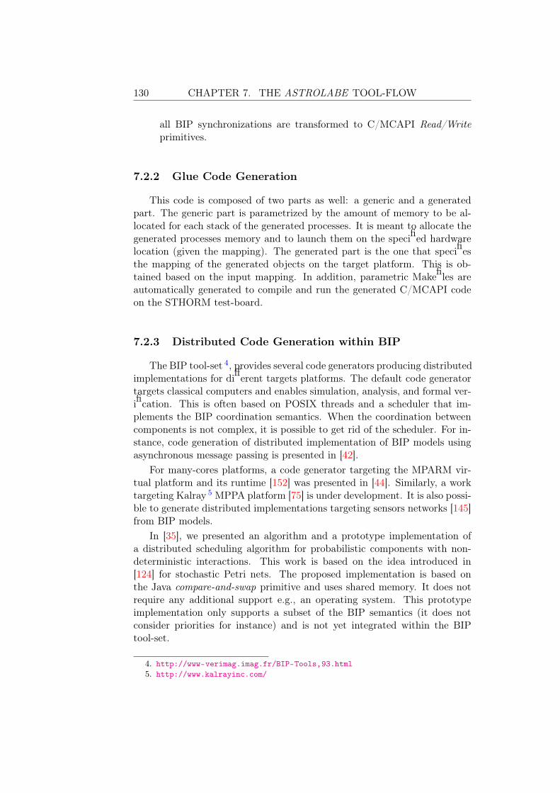
130 CHAPTER 7. THE ASTROLABE TOOL-FLOW
all BIP synchronizations are transformed to C/MCAPI Read/Writeprimitives.
7.2.2 Glue Code Generation
This code is composed of two parts as well: a generic and a generatedpart. The generic part is parametrized by the amount of memory to be al-located for each stack of the generated processes. It is meant to allocate thegenerated processes memory and to launch them on the specified hardwarelocation (given the mapping). The generated part is the one that specifiesthe mapping of the generated objects on the target platform. This is ob-tained based on the input mapping. In addition, parametric Makefiles areautomatically generated to compile and run the generated C/MCAPI codeon the STHORM test-board.
7.2.3 Distributed Code Generation within BIP
The BIP tool-set 4, provides several code generators producing distributedimplementations for different targets platforms. The default code generatortargets classical computers and enables simulation, analysis, and formal ver-ification. This is often based on POSIX threads and a scheduler that im-plements the BIP coordination semantics. When the coordination betweencomponents is not complex, it is possible to get rid of the scheduler. For in-stance, code generation of distributed implementation of BIP models usingasynchronous message passing is presented in [42].
For many-cores platforms, a code generator targeting the MPARM vir-tual platform and its runtime [152] was presented in [44]. Similarly, a worktargeting Kalray 5 MPPA platform [75] is under development. It is also possi-ble to generate distributed implementations targeting sensors networks [145]from BIP models.
In [35], we presented an algorithm and a prototype implementation ofa distributed scheduling algorithm for probabilistic components with non-deterministic interactions. This work is based on the idea introduced in[124] for stochastic Petri nets. The proposed implementation is based onthe Java compare-and-swap primitive and uses shared memory. It does notrequire any additional support e.g., an operating system. This prototypeimplementation only supports a subset of the BIP semantics (it does notconsider priorities for instance) and is not yet integrated within the BIPtool-set.
4. http://www-verimag.imag.fr/BIP-Tools,93.html
5. http://www.kalrayinc.com/
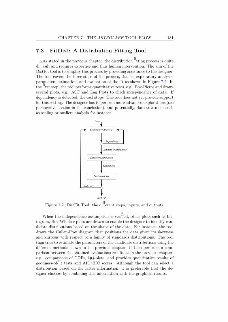
CHAPTER 7. THE ASTROLABE TOOL-FLOW 131
7.3 FitDist: A Distribution Fitting Tool
As stated in the previous chapter, the distribution fitting process is quitedifficult and requires expertise and thus human intervention. The aim of theDistFit tool is to simplify this process by providing assistance to the designer.The tool covers the three steps of the process, that is, exploratory analysis,parameters estimation, and evaluation of the fit as shown in Figure 7.2. Inthe first step, the tool performs quantitative tests, e.g., Box-Pierce and drawsseveral plots, e.g., ACF and Lag Plots to check independence of data. Ifdependency is detected, the tool stops. The tool does not yet provide supportfor this setting. The designer has to perform more advanced explorations (seeperspective section in the conclusion), and potentially, data treatment suchas scaling or outliers analysis for instance.
Parameters Estimation
Fit Evaluation
Dipendency
Cadidate Distributions
Estimations
Best Fit
Bad Fits
Data
Exploratory Analysis
Figure 7.2: DistFit Tool: the different steps, inputs, and outputs.
When the independence assumption is verified, other plots such as his-togram, Box-Whisker plots are drawn to enable the designer to identify can-didate distributions based on the shape of the data. For instance, the tooldraws the Cullen-Fray diagram that positions the data given its skewnessand kurtosis with respect to a family of standards distributions. The toolthen tries to estimate the parameters of the candidate distributions using thedifferent methods shown in the previous chapter. It then performs a com-parison between the obtained evaluations results as in the previous chapter,e.g., comparisons of CDFs, QQ-plots, and provides quantitative results ofgoodness-of-fit tests and AIC/BIC scores. Although the tool can select adistribution based on the latter information, it is preferable that the de-signer chooses by combining this information with the graphical results.

132 CHAPTER 7. THE ASTROLABE TOOL-FLOW
The tool is built in the R 6 statistical environment [196]. It uses a specificpackage called fitdistrplus, that offers various facilities for fitting a distribu-tion to a set of input data [80], in addition to the lawstat package[116] forspecific statistical tests.
7.4 Stochastic Abstraction Tool
As explained in Chapter 4, the stochastic abstraction is mainly basedon machine learning algorithms. The illustrated results are based on theAAlergia algorithm [153], for which a Matlab implementation is provided 7.We built upon this existing work and implemented the projection phase ofthe stochastic abstraction in Python. We created a set of scripts that, givena set of input strings and the support of an LTL property φ, i.e., the setof symbols explicitly appearing in φ, produces a set of projected strings byreplacing the irrelevant symbols in the strings by a special symbol.
7.5 BIPSMC: An SMC Engine for SBIP Models
S Simulator - executable -
BIP Compilation
Φ Monitor - executable -
SMC Core SSP / SPRT / PESTIM
- executable -
System S -SBIP -
OK / KO trace
verdict
Final Verdict
execution trace
Property Φ - PBLTL -
PBLTL Compilation
Parameters δ , (α , β)
triggers
produces
collects trace length n
Figure 7.3: BIPSMC tool architecture: diagram of the main modules.
The BIPSMC tool implements several statistical testing algorithms forstochastic systems verification, namely, Single Sampling Plan (SSP), Sim-
6. http://www.r-project.org/
7. http://mi.cs.aau.dk/code/aalergia/

CHAPTER 7. THE ASTROLABE TOOL-FLOW 133
ple Probability Ratio Test (SPRT) [205, 209], and Probability Estimation(PESTIM) [110]. Figure 7.3 shows the most important modules of the tooland how they interact in order to perform statistical model checking. Thetool takes as inputs a stochastic model description in SBIP format, a PBLTLproperty to check, and a series of confidence parameters needed by the statis-tical test. During an initial phase, the tool performs a syntactic validationof the PBLTL formula through a parser module. Then, it builds an exe-cutable model and a monitor for the property under verification. Next, itwill iteratively trigger the stochastic BIP engine to generate independentexecution traces which are monitored to produce local verdicts. This pro-cedure is repeated until a global decision can be taken by the SMC coremodule (that implements the statistical algorithms). As our approach relieson SMC and since it considers bounded LTL properties, we are guaranteedthat the procedure will eventually terminate.
7.5.1 SBIP Modeling Language
We consider the following example of binary signal generator to illustratethe SBIP modeling language. Figure 7.4 shows a DTMC model of the gen-erator and its corresponding SBIP model. The textual description of thiscomponent is given hereafter.
/* Declares an atomic component */
atomic type binary_generator
data int v0, v1 // Declares probabilistic variables
data distribution_t d0 // Declares probabilistic distributions
...
export port Port print_0() // Declares and exports ports
...
place l0, l1, l0’, l1’ // Declares BIP locations
initial to l0 do {
d0 = init_distribution(’distribution0.txt’); // Initialize d0
... }
...
on internal from l0 to l0’ do { // Transition from l0 to l0’
v0 = select(d0); // Update v0 w.r.t. d0
}
/* Transition from l0’ to l0 */
on print_0 from l0’ to l0 provided (v0 == 0)
/* Transition from l0’ to l1 */
on print_1 from l0’ to l1 provided (v0 == 1)
...
end
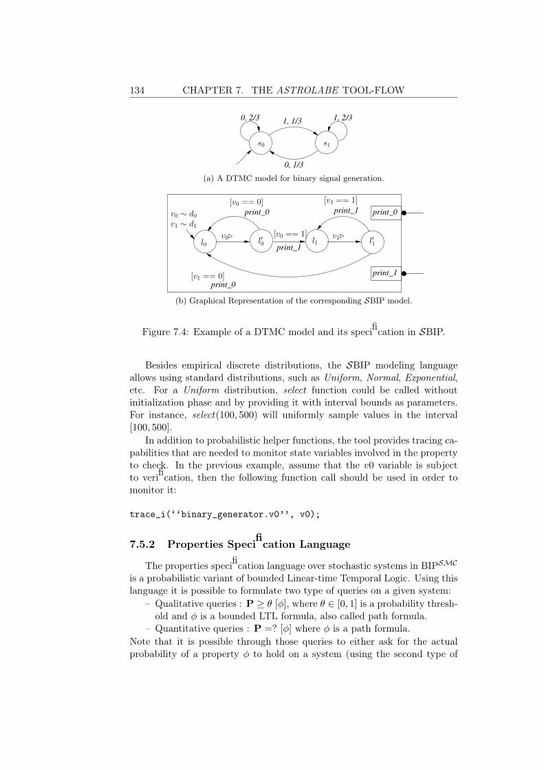
134 CHAPTER 7. THE ASTROLABE TOOL-FLOW
1, 1/3
0, 1/3
1, 2/30, 2/3
s1s0
(a) A DTMC model for binary signal generation.
print_0 print_1
print_0
print_1
print_1
print_0
l0 l1v0� l�1
[v0 == 1]
[v0 == 0] [v1 == 1]
l�0v1�
[v1 == 0]
v0 ∼ d0v1 ∼ d1
(b) Graphical Representation of the corresponding SBIP model.
Figure 7.4: Example of a DTMC model and its specification in SBIP.
Besides empirical discrete distributions, the SBIP modeling languageallows using standard distributions, such as Uniform, Normal, Exponential,etc. For a Uniform distribution, select function could be called withoutinitialization phase and by providing it with interval bounds as parameters.For instance, select(100, 500) will uniformly sample values in the interval[100, 500].
In addition to probabilistic helper functions, the tool provides tracing ca-pabilities that are needed to monitor state variables involved in the propertyto check. In the previous example, assume that the v0 variable is subjectto verification, then the following function call should be used in order tomonitor it:
trace_i(‘‘binary_generator.v0’’, v0);
7.5.2 Properties Specification Language
The properties specification language over stochastic systems in BIPSMC
is a probabilistic variant of bounded Linear-time Temporal Logic. Using thislanguage it is possible to formulate two type of queries on a given system:
– Qualitative queries : P ≥ θ [φ], where θ ∈ [0, 1] is a probability thresh-old and φ is a bounded LTL formula, also called path formula.
– Quantitative queries : P =? [φ] where φ is a path formula.
Note that it is possible through those queries to either ask for the actualprobability of a property φ to hold on a system (using the second type of

CHAPTER 7. THE ASTROLABE TOOL-FLOW 135
queries) or to determine if the property satisfies some threshold θ (using thefirst type of queries).
Path formulas, in SBIP, are defined using four bounded temporal oper-ators namely, Next (N{l} ψ), Until (ψ1U{l} ψ2), Eventually (F{l} ψ), andAlways (G{l} ψ) where l is an integer value that specify the length of thetrace to consider and ψ,ψ1,ψ2 are called state formulas, that is, Booleanpredicates evaluated on system state. For example, the following PBLTLformula
P =?[G{1000}(abs(Master.tm− Slave.ts) ≤ 160)]
asks "what is the probability that the absolute value of the difference betweenvariable tm and variable ts is always under the bound 160 ?".
In this example, the path formula is
G{1000}(abs(Master.tm− Slave.ts) ≤ 160)
and the state formula is abs(Master.tm−Slave.ts) ≤ 160. Variables namesare always specified as component_name.variable_name. Note that SBIPgives the possibility to use built-in predefined mathematical functions instate formulas. For the example above, abs() function is called to computethe absolute value of the difference between tm and ts.
Monitoring LTL Properties
For applying statistical model checking on stochastic systems it is manda-tory to be able to evaluate the BLTL property under consideration on systemexecution traces. Indeed, this monitoring operation shall generate binary ob-servations xi = {0, 1} (single trace verdict) which are requested by the sta-tistical algorithms to provide a global verdict that concerns the whole system(final verdict). In theory, monitoring consists to check if some word (labelingthe current execution trace) belongs to the language generated by some au-tomaton encoding the property. Actually, there exist an important researchliterature about the efficient transformation from LTL to Buchi [93, 208] oralternating [201] automata. Some of these works cover bounded LTL [89, 94].
In BIPSMC , we syntactically restricted BLTL to a fragment where thetemporal operators cannot be nested. This simplification restricts the defini-tion to a finite number of automata patterns that covers all property classes.Moreover, this fragment has been expressive enough to cover all propertiesof interest in practical applications. Furthermore, it is always possible toenrich this set with additional patterns, as needed.
7.5.3 Technical details and Tool Availability
BIPSMC is fully developed in Java programming language. It uses JEP2.4.1 library 8 (under GPL license) for parsing and evaluating mathemati-
8. http://www.singularsys.com/jep/

136 CHAPTER 7. THE ASTROLABE TOOL-FLOW
cal expressions and ANTLR 3.2 9 for PBLTL parsing and monitoring. Atthis stage, BIPSMC only runs on GNU/Linux operating systems since it iscoupled to BIP. The first release of the tool only works on command linemode. We are working on a graphical user interface that will be availablein the next release. The model checker can be downloaded from http:
//www-verimag.imag.fr/Statistical-Model-Checking.html, where youcan find additional resources on how to install it and use it with the BIPframework.
7.6 Integration within the BIP Design Flow
The presented tool-flow completes a set of already existing tools withinthe BIP design flow. This offers a rigorous approach for tackling embeddedsystems design challenges. As shown in Figure 7.5, it offers an ensemble oftools for formal modeling, model transformations, formal verification, andcode generation. We present hereafter the one which are in direct relationwith the present work.
7.6.1 DOL and DOL2BIP
DOL stands for Distributed Operation Layer [198]. It is a frameworkdevoted to the specification and analysis of mixed hardware/software sys-tems. DOL provides languages for the representation of particular classes ofapplications software, multi-processor architectures and their mappings. InDOL, application software is defined using a variant of Kahn process net-work [95] model. It consists of a set of deterministic, sequential processes (inC) communicating asynchronously through FIFO channels. The hardwarearchitecture is described as interconnections of computational and commu-nication resources such as processors, buses and memories. The mappingassociates application software components to resources of the hardware ar-chitecture, that is, processes to processors and FIFO channels to memories.
DOL2BIP [44] is a tool that transforms DOL specifications into BIPmodels. Figure 7.6 shows a KPN model composed of six processes, namelyConfig, Splitter, Joiner, and three Worker instances. The communicationbetween these processes is based on blocking Read/Write primitives on FIFOchannels following the DOL semantics. In this example, the initial stepconsists of configuring (data size, data type, etc.) the Worker processes.It is performed by the Config process. Generic processes are considered toenable the processing of different data types/sizes. After configuration, thedata to be processed is split and sent by the Splitter to the workers that runin parallel. Finally, the results is collected by the Joiner.
9. http://www.antlr3.org/

CHAPTER 7. THE ASTROLABE TOOL-FLOW 137
Applica'on Model -‐BIP-‐
Mapping -‐XML-‐
1 -‐ Code Genera2on
2 -‐ Sta2s2cal Inference
Target Pla3orm
Applica'on Executable(s)
3 -‐ Model Calibra2on
5 -‐ Sta2s2cal Model Checking
System Requirements
Execu'on Traces
Architecture Model -‐BIP-‐
4 -‐ Stochas2c Abstrac2on
Performance Modeling Performance Evalua'on
System Model -‐BIP-‐
Prob. Perf. Characteriza'on
Performance Model -‐SBIP-‐
Abstract Perf. Model -‐SBIP-‐
BIP2MCAPI
FitDist
BIPSMC
Abstractor
KPN Applica'on Model (C + XML)
Mapping (XML)
Architecture Model (XML)
DOL
D-‐Finder
Func'onal Results
BIP Hw Components
Library
DOL2BIP
BIPWeaver
Quan'ta've Perf. Feedback
Figure 7.5: The ASTROLABE tool-flow extended with several tools: DOL,DOL2BIP, BIPWeaver, the BIP Hw library, and D-Finder.
Splitter
Worker
Worker Joiner
Worker
Config
Figure 7.6: A KPN model example consisting of a split/join schema: Asplitter, Several parallel workers, and a joiner process.
Given the KPN model in Figure 7.6, the generation of the correspondingBIP representation is straightforward. As shown in Figure 7.7, each processis transformed to an atomic BIP component modeled as an extended automa-ton following the BIP formalism. Additional components modeling commu-nication through FIFOs are explicitly introduced. In each BIP componentcorresponding to a DOL process, the DOL Read/Write calls are transformed
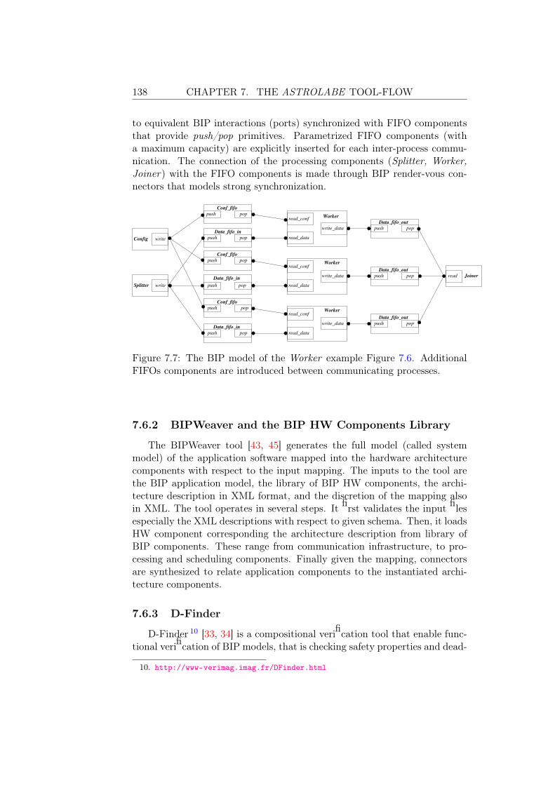
138 CHAPTER 7. THE ASTROLABE TOOL-FLOW
to equivalent BIP interactions (ports) synchronized with FIFO componentsthat provide push/pop primitives. Parametrized FIFO components (witha maximum capacity) are explicitly inserted for each inter-process commu-nication. The connection of the processing components (Splitter, Worker,Joiner) with the FIFO components is made through BIP render-vous con-nectors that models strong synchronization.
read_data
read_conf
write_data
read_data
read_conf
write_data
Worker
read_data
read_conf
write_data
Worker
writeSplitter
push pop
Data_fifo_out
push pop
Data_fifo_out
push pop
Data_fifo_out
read Joiner
Worker
push
push
pop
pop
push pop
Conf_fifo
push pop
poppush
Conf_fifo
Conf_fifo
writeConfig push pop
Data_fifo_in
Data_fifo_in
Data_fifo_in
Figure 7.7: The BIP model of the Worker example Figure 7.6. AdditionalFIFOs components are introduced between communicating processes.
7.6.2 BIPWeaver and the BIP HW Components Library
The BIPWeaver tool [43, 45] generates the full model (called systemmodel) of the application software mapped into the hardware architecturecomponents with respect to the input mapping. The inputs to the tool arethe BIP application model, the library of BIP HW components, the archi-tecture description in XML format, and the discretion of the mapping alsoin XML. The tool operates in several steps. It first validates the input filesespecially the XML descriptions with respect to given schema. Then, it loadsHW component corresponding the architecture description from library ofBIP components. These range from communication infrastructure, to pro-cessing and scheduling components. Finally given the mapping, connectorsare synthesized to relate application components to the instantiated archi-tecture components.
7.6.3 D-Finder
D-Finder 10 [33, 34] is a compositional verification tool that enable func-tional verification of BIP models, that is checking safety properties and dead-
10. http://www-verimag.imag.fr/DFinder.html

CHAPTER 7. THE ASTROLABE TOOL-FLOW 139
lock freedom. It uses an abstraction technique based on invariant and reach-ability analysis to avoid exhaustive and costly verification. To this end, itenables an efficient generation of components and communication invariant.The tool has been used to verify several case-studies and has been recentlyextended to invariant generation of timed models [10].
7.7 Conclusions
In this chapter, we presented a tool-flow implementation associated withthe ASTROLABE approach introduced in Chapter 5. The goal of this tool-flow is to enable rigorous and especially automatic performance modelingand analysis at system-level. We mainly presented a code generator forthe STHORM platform and the MCAPI runtime, denoted BIP2MCAPI, anassistance tool for distribution fitting, an automatic way to build stochasticabstractions, and a statistical model checker, namely BIPSMC .
The BIPSMC model checker consists of 22 Java classes summing up to∼ 3500 lines of code (loc), the BIP2MCAPI code generator consists of 7 Javaclasses summing up to ∼ 1740 loc, and the DistFit tool is one R file thatcontains about 650 loc. As stated earlier, the stochastic abstraction toolis based on an existing Matlab implementation of the AAlergia algorithm.We implemented on top of it a set of Python scripts for the projection partwhich is about 130 loc.
In the next and last chapter of this part, we present a case study thatillustrates the use of the ASTROLABE approach and the associated tool-flow. The case study consists of an image recognition application runningon a many-cores platform.


Chapter 8Image Recognition on Many-cores
In this chapter we illustrate the use of the ASTROLABE approach andits associated tool-flow for the design of an embedded system for image recog-nition and contour detection. The application part of this system consists ofthe HMAX models algorithm for object recognition that operates on severalsteps as detailed hereafter. In this case study, the architecture part is com-pletely specified and consists of a many-cores platform, namely STHORM.With reference to the possible design configurations (see Section 1.2.3 inIntroduction), this falls within the second setting, where the goal is to effi-ciently design and map the application into the specified architecture. Forthis case study, we will be considering timing as the main efficiency criterion.
8.1 Application Overview
HMAX models algorithm [160] is a hierarchical computational model ofobject recognition which attempts to mimic the rapid object recognition ofhuman brain. Hierarchical approaches to generic object recognition have be-come increasingly popular over the years, they indeed have been shown toconsistently outperform flat single-template (holistic) object recognition sys-tems on a variety of object recognition task. Recognition typically involvesthe computation of a set of target features at one step, and their combinationin the next step. A combination of target features at one step is called alayer, and can be modeled by a 3D array of units which collectively repre-sent the activity of set of features (F) at a given location in a 2D input grid.HMAX starts with an image layer of gray scale pixels (a single feature layer)and successively computes higher layers, alternating “S” and “C” layers:
– Simple (“S”) layers apply local filters that compute higher-order fea-tures by combining different types of units in the previous layer.
– Complex (“C”) layers increase invariance by pooling units of the sametype in the previous layer over limited ranges. At the same time, the
141
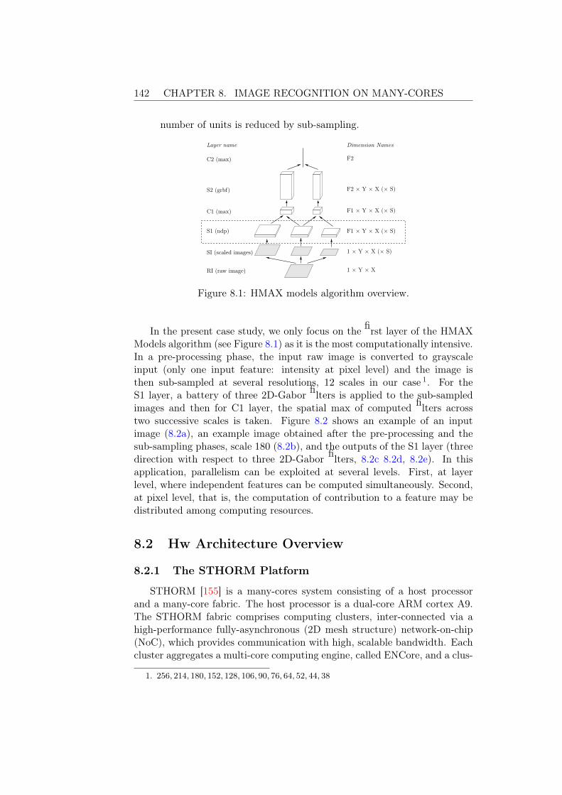
142 CHAPTER 8. IMAGE RECOGNITION ON MANY-CORES
number of units is reduced by sub-sampling.
1 × Y × X
1 × Y × X (× S)
F1 × Y × X (× S)
F1 × Y × X (× S)
F2 × Y × X (× S)
F2
Dimension Names
C2 (max)
S2 (grbf)
C1 (max)
S1 (ndp)
SI (scaled images)
Layer name
RI (raw image)
Figure 8.1: HMAX models algorithm overview.
In the present case study, we only focus on the first layer of the HMAXModels algorithm (see Figure 8.1) as it is the most computationally intensive.In a pre-processing phase, the input raw image is converted to grayscaleinput (only one input feature: intensity at pixel level) and the image isthen sub-sampled at several resolutions, 12 scales in our case 1. For theS1 layer, a battery of three 2D-Gabor filters is applied to the sub-sampledimages and then for C1 layer, the spatial max of computed filters acrosstwo successive scales is taken. Figure 8.2 shows an example of an inputimage (8.2a), an example image obtained after the pre-processing and thesub-sampling phases, scale 180 (8.2b), and the outputs of the S1 layer (threedirection with respect to three 2D-Gabor filters, 8.2c 8.2d, 8.2e). In thisapplication, parallelism can be exploited at several levels. First, at layerlevel, where independent features can be computed simultaneously. Second,at pixel level, that is, the computation of contribution to a feature may bedistributed among computing resources.
8.2 Hw Architecture Overview
8.2.1 The STHORM Platform
STHORM [155] is a many-cores system consisting of a host processorand a many-core fabric. The host processor is a dual-core ARM cortex A9.The STHORM fabric comprises computing clusters, inter-connected via ahigh-performance fully-asynchronous (2D mesh structure) network-on-chip(NoC), which provides communication with high, scalable bandwidth. Eachcluster aggregates a multi-core computing engine, called ENCore, and a clus-
1. 256, 214, 180, 152, 128, 106, 90, 76, 64, 52, 44, 38

CHAPTER 8. IMAGE RECOGNITION ON MANY-CORES 143
(a) Input image (b) Sampled grayscale image
(c) Output imagedirection 1
(d) Output imagedirection 2
(e) Output imagedirection 3
Figure 8.2: Example of input and output images of the HMAX S1 layer.
ter controller (CC). The ENCore embeds a set of tightly-coupled processorelements (PE) which are customizable 32-bit STxP70-v4 RISC processorsfrom ST Microelectronics. On the STHORM test-board used in our exper-iments, the fabric comprises 4 clusters, with 16 PEs each. The PEs in onecluster share a multi-banked level-1 (L1) data memory of 256 KBytes. Thebanks of the L1 memory can be accessed in parallel in one processor cycle.Each PE has its private instruction cache with a size of 16 KBytes.
The CC consists of a cluster core (STxP70-v4), a multi-channel advancedDMA engine, and specialized hardware for synchronization. The latter twoare accessible also by the PEs. The CC interconnects with two interfaces: oneto the ENCore and one to the asynchronous NoC. All clusters share 1 MByteof level-2 (L2) memory, accessible via the NoC. The access time is severaltens of cycles. A DDR3 level-3 (L3) memory is available off-chip (1 GByte);this memory has a large size, however its access time and bandwidth aremuch slower than the ones of the on-chip memory.
In summary, due to area and power constraints, the fast memory availableon the chip is scarce. Furthermore, the host processor and the cores on thefabric have a different instruction-set-architecture. These two aspects makeefficient programming on STHORM a challenging task.
8.2.2 The Multi-core Communication API
The main objective of the MCAPI implementation on STHORM is tooffer a homogeneous programming interface for the entire platform (fabricand host). This uniform representation covering the entire platform can per-fectly integrate the full design flow targeting STHORM, which significantly

144 CHAPTER 8. IMAGE RECOGNITION ON MANY-CORES
eases code generation and analysis. The current MCAPI implementationfeatures five domains: one for each cluster on the fabric, and one for thehost as shown in Figure 8.3.
Figure 8.3: MCAPI domains on STHORM.
The five domains naturally reflect the STHORM hardware organization.Furthermore, in each cluster-domain each MCAPI node is mapped on a PE.The host-domain has only a single node corresponding to the ARM dual-core processor. The host node is responsible for the deployment of the entireexecution, as it is the main entry point of an application. The MCAPI ini-tialization of the host node automatically loads the fabric binary code intothe L2 memory, and starts the fabric MCAPI nodes. The MCAPI imple-mentation totally hides from application the complexity dynamic loading ofof binary and symbols dependency solution. A single semantic for the entireSTHORM platform is exposed for homogeneous programming.
The channels are implemented using FIFO buffers allocated in any of thememory levels available on STHORM. The size of the allocated buffer andits memory placement can be set by using endpoint attributes, as specifiedin the MCAPI standard. The sending endpoint and the receiving endpointmust have consistent attributes definition for the creation of a channel. NoMCAPI node is mapped on the CCs, meaning that they are not directlyvisible to the programmer. Instead, they are used internally in the MCAPIimplementation to support the various communication mechanisms and syn-chronizations. DMA engines are also hidden from the programmer, but usedby the implementation to transfer data between memory levels and domains.
8.3 Performance Requirements Overview
As stated in the beginning of this chapter, we will mainly focus on thetiming dimension of the system, which will constitute the efficiency criterion.We are interested on the overall execution time and the time to process single

CHAPTER 8. IMAGE RECOGNITION ON MANY-CORES 145
lines of the input image. More precisely, we will compute the probabilitiesthat the overall execution time is always lower than a given bound Δ and thatthe variability in the processing time of successive lines is always boundedby Ψ . To this end, we specify the above requirements in BLTL as follows:
1. Overall execution time: φ1 = Gl(t < Δ), where t is the monitoredoverall execution time.
2. Variability of the time of processing successive lines : φ2 = Gl(|tl| < Ψ),where tl is the difference between the processing time of successivelines.
8.4 Functional and Performance Modeling
8.4.1 High-Level Reconfigurable KPN Model
We developed a parametric KPN model for the S1 layer of HMAX inDOL. The model is based on the worker pattern presented previously. Ituses a certain number of reconfigurable processes for implementing the 2D-Gabor filtering and image splitting/joining. Every image is handled by oneprocessing group consisting of one Splitter, one or more Gabor (Worker)and one Joiner, connected through blocking FIFO channels as illustratedin Figure 8.4. This model exploits parallelism both at image level, as dif-ferent images are processed in parallel by different processing groups andat pixel level, as different stripes of the image are processed in parallel bydifferent Gabor processes. Moreover, parallelism is exploited between purecomputation on Gabor processes and data transfer from/to main memoryby Splitter/Joiner processes.
Gabor
Gabor
Gabor
… x 14
Splitter Joiner Main
246
Gabor
Gabor
Gabor
… x 14
Splitter Joiner
Gabor
Gabor
Gabor
… x 6
Splitter Joiner
Main
106
180
204
152
128
90
76
64
52
44
38
170
142
118
96
80
66
54
42
34
28
256 214
Processing Group
Host Host
Processing Group
Processing Group
Figure 8.4: An abstract view of the S1 layer of HMAX models algorithm.

146 CHAPTER 8. IMAGE RECOGNITION ON MANY-CORES
The computation of the entire S1 layer is coordinated by a single mainprocess. Several image scales are handled concurrently. That is, the twelvescaled images are statically pre-allocated and mapped on different processinggroups. For every image scale, the processing is pipelined as follows. Initially,the main process sends the first 10 + P lines to the corresponding processinggroup, where P ≥ 0 is an integer parameter called line pressure that specifiesthe pipelining rate. In normal regime, one input line is sent and one outputline is received, for every filter rotation (that is, actually three output lines).Finally, once all the input image has been sent, the main process receives Pmore output lines. At this point, the processing group is ready (empty) andcan be reconfigured to restart computation for another image scale.
/** DOL Gabor Process **/
void gabor_init()
{ status = CONFIG; }
void gabor_fire(){
if(status == CONFIG){
/* Read configuration parameters
from input configuration FIFO */
read(CONF_FIFO, &config);
/* Update number of steps */
step = config.step;
/* Update status */
status = EXEC; }
if(status == EXEC){
/* Read data from input data FIFO */
read(DATA_FIFO_IN, &data);
/* Execute computation function */
compute_filter(&data);
/* Write data to output FIFO */
write(DATA_FIFO_OUT, data);
/* Update number of steps */
step--;
/* Update status */
if(step == 0) status = CONFIG;
}
}
Within the processing group, the Splitter receives input images, line byline from the main process. Every line is split into a number of equal length(and overlapping) fragments, one for every Gabor process, and sent to theseprocesses. Gabor processes implement the computation of the 2D-filter itself(A DOL code sample of the Gabor process is given above). Filter size is fixedto 11 × 11 in the case study. Hence, Gabor processes need to accumulate 11

CHAPTER 8. IMAGE RECOGNITION ON MANY-CORES 147
line fragments in order to perform computation. Henceforth, they maintainand compute the result operating on an internal "sliding" window of 11 linefragments. Finally, the resulting fragments are sent further to the Joiner,which packs them into complete output lines and sends them to the mainprocess.
In this experiment, for the sake of simplicity, we only consider one imagescale (256×256), that is, one processing group will be actually used as shownin Figure 8.5. Besides, reducing the model size, this restriction relaxes data-dependency since a single input size is considered. It is worth mentioningthat, given one image scale as input, each process will always handle the sameworkload (amount of data) which increases the statistical learning confidence.
Gabor
Gabor
Gabor
… x 14
Splitter Joiner Main 246
Main 256
Cluster
Host Host
Figure 8.5: The simplified model of the S1 layer of HMAX models algorithm.
Given the KPN model above, we generate a BIP model using the DOL2BIPtool described in the previous section. We depict in Figure 8.6 the obtainedBIP component for the Gabor process, which consists of an automaton thatreproduces the behavior described earlier. That is, a configuration step in l0given the configuration data (this specifies for instance the number of frag-ment to process denoted steps in Figure 8.6), followed by several iterations(from l1 to l4, which depends on the number of steps to perform) consistingof reading a fragment from the input queue DATA_FIFO_IN, computingthe filer, and writing the results into the output queue DATA_FIFO_OUT.The DOL2BIP transformation produces in addition FIFO components, asdescribed earlier. Figure 8.7 shows such a component.
write_data
compute_filter(&data)
read(DATA_FIFO_IN, &data)
read_data
[steps != 0]
steps−−
[status==EXEC]
[steps == 0]
status = CONFIG
data
write_data
read(CONF_FIFO, &config)
status = EXEC
steps = config.steps
read_conf
[status == CONFIG]
data
write(DATA_FIFO_OUT, data)read_conf
configread_data
status = CONFIG
l0 l1 l2
l3l4
Figure 8.6: A functional BIP model of the Gabor process.

148 CHAPTER 8. IMAGE RECOGNITION ON MANY-CORES
data
receive
data
b = new Queue(max)push(b, data);
receive
[b.size < max]
send
[b.size > 0]
pop(b,&data);
send
l0
Figure 8.7: A BIP model of a FIFO buffer.
Once we generate the functional BIP model of the application, we pro-duce a distributed implementation using the BIP2MCAPI code generatortool. Note that in this case study we are not producing a complete systemmodel (composed of the application mapped to the architecture) as describedin in Chapter 5. Since we are given the target platform, we are not consid-ering a model of the architecture but only a model of the application and amapping. A sample of generated code, corresponding to the Gabor process,is shown below. The produced code is instrumented in order to observe ex-ecution and communication time of each process. In this case study, we relyon a physical STHORM test-board in order to gather low-level performancedata. The generated implementation is therefore deployed and executed andthe corresponding performance traces can be directly produced.
void gabor_ins_execute(void* args) {
/* Initialization part */
...
/* Behavior part */
while(Wlcontinue){
switch(BIP_CTRL_LOC){
case L0 : {
if (status == CONFIG){ ...
status = EXEC; BIP_CTRL_LOC = S0; }
if (status == EXEC) BIP_CTRL_LOC = S1;
break; }
case L1 : {
mcapi_pktchan_recv(h_WORKER_read_data, (void**)&mcapi_buffer,
&mcapi_received, &mcapi_status);
if((mcapi_received != size) || (mcapi_status != MCAPI_SUCCESS))
ERR_RAISE("FAIL TO READ DATA");
memcpy(data, mcapi_buffer, mcapi_received);
size = mcapi_received;
mcapi_pktchan_release(mcapi_buffer, &mcapi_status);
if(mcapi_status != MCAPI_SUCCESS) ERR_RAISE("FAIL TO RELEASE CHANNEL");
BIP_CTRL_LOC=S2 ;
break; }
case L2 : {
compute(&data); BIP_CTRL_LOC=S3;
break; }

CHAPTER 8. IMAGE RECOGNITION ON MANY-CORES 149
case L3 : {
mcapi_pktchan_send(h_WORKER_write_data, data, size, &mcapi_status);
if(mcapi_status != MCAPI_SUCCESS) ERR_RAISE("FAIL TO SEND DATA");
step--; BIP_CTRL_LOC=S4;
break; }
...
}
}
}
8.4.2 Performance Characterization and Model Calibration
Now that we dispose of execution traces that concern the performancedimension of interest, that is time, we apply the distribution fitting processto learn probability distributions that characterizes these data. We illustratethe different steps of the process on the execution time of the Gabor process.Exploratory Analysis is first performed to observe if the data provide anyclues to resemble to a standard probability distribution. Runs and Box plotsare initially used to observe the data shape and evolution. The corresponding
66
56
70
67
56
80
Exe
c. T
ime
(u
s)
0 200 400 600 800
66
56
70
67
56
80
Observation Index
Exe
c. T
ime
(u
s)
Figure 8.8: Box-Whisker and Runs plots of the Gabor execution time. Ex-treme observations correspond to the end of the process execution.
plots are presented in Figure 8.8, which reveal the presence of very extremevalues clearly deviating from the other observations, these are considered asoutliers 2 and are eliminated from the sample under study. Figure 8.9 showsthe same plots after removing outliers.
2. http://www.itl.nist.gov/div898/handbook/eda/section3/eda35h.htm

150 CHAPTER 8. IMAGE RECOGNITION ON MANY-CORES
67
6.0
67
6.5
67
7.0
67
7.5
67
8.0
67
8.5
67
9.0
Exe
c. T
ime
(u
s)
0 200 400 600 800
67
6.0
67
6.5
67
7.0
67
7.5
67
8.0
67
8.5
67
9.0
Observation IndexE
xe
c. T
ime
(u
s)
Figure 8.9: Box-Whisker and Runs plots of the Gabor execution time obser-vations after outlier elimination (observation are more compact).
676.0 676.5 677.0 677.5 678.0 678.5 679.0
67
66
77
67
86
79
lag 1
da
ta
Figure 8.10: Lag plot of the Gabor execution time observations. It showsrandom spread of the data (no specific shape is appearing).
To check if the data observations are independent, we first use the Lagplot. This draws the observations xi in the y-axis and xj in the x-axis,where i− j is the fixed lag. For instance, Figure 8.10 shows the Lag plot ofthe Worker execution time with lag equal to 1. The figure clearly shows arandom dispersion of the observations. To get more confidence, we used the
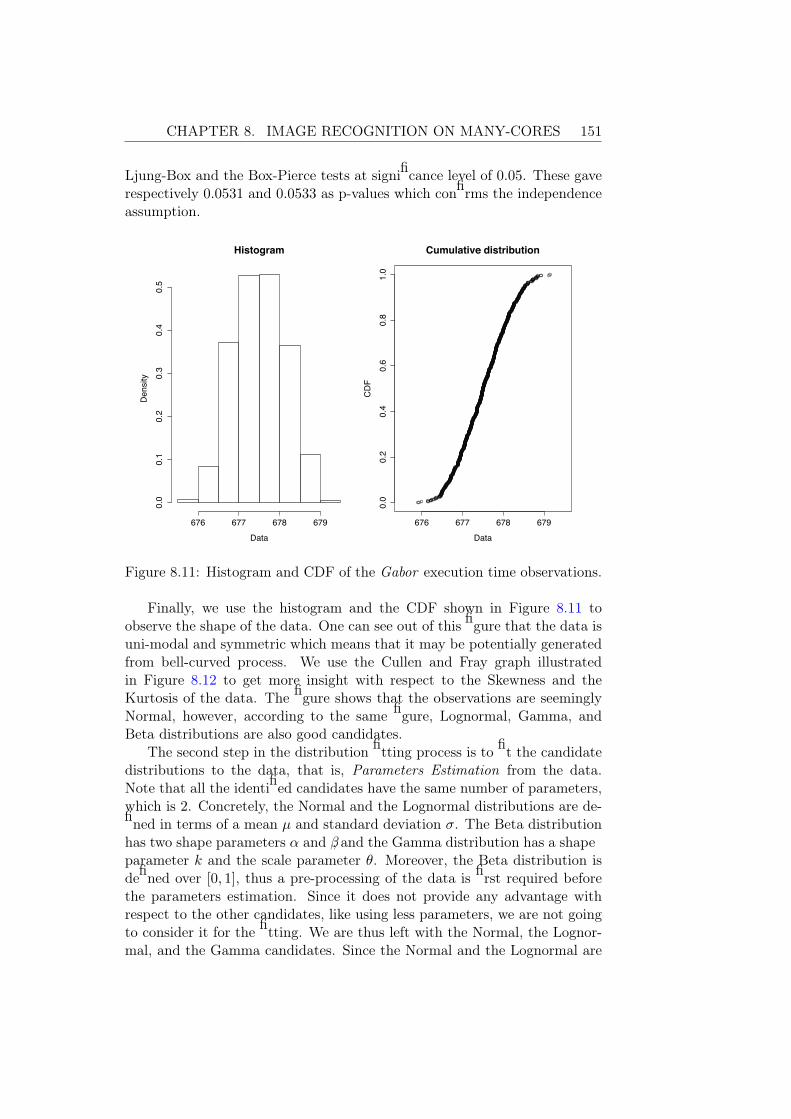
CHAPTER 8. IMAGE RECOGNITION ON MANY-CORES 151
Ljung-Box and the Box-Pierce tests at significance level of 0.05. These gaverespectively 0.0531 and 0.0533 as p-values which confirms the independenceassumption.
Histogram
Data
Density
676 677 678 679
0.0
0.1
0.2
0.3
0.4
0.5
676 677 678 679
0.0
0.2
0.4
0.6
0.8
1.0
Cumulative distribution
Data
CDF
Figure 8.11: Histogram and CDF of the Gabor execution time observations.
Finally, we use the histogram and the CDF shown in Figure 8.11 toobserve the shape of the data. One can see out of this figure that the data isuni-modal and symmetric which means that it may be potentially generatedfrom bell-curved process. We use the Cullen and Fray graph illustratedin Figure 8.12 to get more insight with respect to the Skewness and theKurtosis of the data. The figure shows that the observations are seeminglyNormal, however, according to the same figure, Lognormal, Gamma, andBeta distributions are also good candidates.
The second step in the distribution fitting process is to fit the candidatedistributions to the data, that is, Parameters Estimation from the data.Note that all the identified candidates have the same number of parameters,which is 2. Concretely, the Normal and the Lognormal distributions are de-fined in terms of a mean µ and standard deviation σ. The Beta distributionhas two shape parameters α and β, and the Gamma distribution has a shapeparameter k and the scale parameter θ. Moreover, the Beta distribution isdefined over [0, 1], thus a pre-processing of the data is first required beforethe parameters estimation. Since it does not provide any advantage withrespect to the other candidates, like using less parameters, we are not goingto consider it for the fitting. We are thus left with the Normal, the Lognor-mal, and the Gamma candidates. Since the Normal and the Lognormal are

152 CHAPTER 8. IMAGE RECOGNITION ON MANY-CORES
0 1 2 3 4
Cullen and Frey graph
square of skewness
ku
rto
sis
10
98
76
54
32
1 Observation Theoretical distributions
normal
uniform
exponential
logistic
beta
lognormal
gamma
(Weibull is close to gamma and lognormal)
Figure 8.12: Cullen and Frey graph for the Gabor execution time.
quite similar 3, we only consider the Normal and the Gamma distributions aspertinent candidates for the fitting process. Observe that the above choicesare mostly subjective and are mainly based on human interpretation.
We now move to estimate the parameters of the retained candidates. Tothis end, we used the method of moment (MME) described in the previouschapter, which gives the following estimates:
– For the Normal candidate: µ = 677.52µs and σ = 0.626µs.– For the Gamma candidate: k = 1172721.38µs and θ = 1730.909µs
The final step in this fitting process is to Evaluate the Obtained Fitsthrough a goodness-of-fit test. We used the different test statistics describedin the previous chapter, that is, Kolmogorv-Smirnov (K-S), Carmer-VonMises (C-VM), and Anderson-Darling (A-D), for which the results are givenin Table 8.1.
K-S C-VM A-D AIC BIC
Normal 0.0331 0.1931 1.342 1398.534 1407.731
Gamma 0.0330 0.1930 1.340 1398.517 1407.714
Table 8.1: Goodness of fit evaluation results for the Normal and the Gammadistributions.
3. They can be obtained from each other using a Log transformation.

CHAPTER 8. IMAGE RECOGNITION ON MANY-CORES 153
The goodness-of-fit tests were performed at a significance level of 0.05. InTable 8.1, two results out of three (Carmer-Von Mises (C-VM) and Anderson-Darling (A-D)) show that both candidates provide good fits, since the ob-tained p-values in each case are greater that 0.05. Thus the we cannotreject the hypothesis stating that the data is normally distributed withµ = 677.52µs and σ = 0.626µs, neither the hypothesis stating that thedata follows a Gamma distribution with k = 1172721.38 and θ = 1730.909.In Table 8.1, we give in addition the obtained AIC and the BIC scores, whichare very similar in this case and do not help us to select. We rely on addi-tional plots to visually compare the two candidates. In Figure 8.13, we show
Histogram and theoretical densities
data
Density
676.0 676.5 677.0 677.5 678.0 678.5 679.0
0.0
0.1
0.2
0.3
0.4
0.5
0.6
NormalGamma
(a) Comparison of PDFs
676.0 676.5 677.0 677.5 678.0 678.5 679.0
0.0
0.2
0.4
0.6
0.8
1.0
Empirical and theoretical CDFs
data
CDF
NormalGamma
(b) Comparison of CDFs
Figure 8.13: Graphical comparison between the Normal and the Gamma fits.The obtained curves for both fits are very similar.
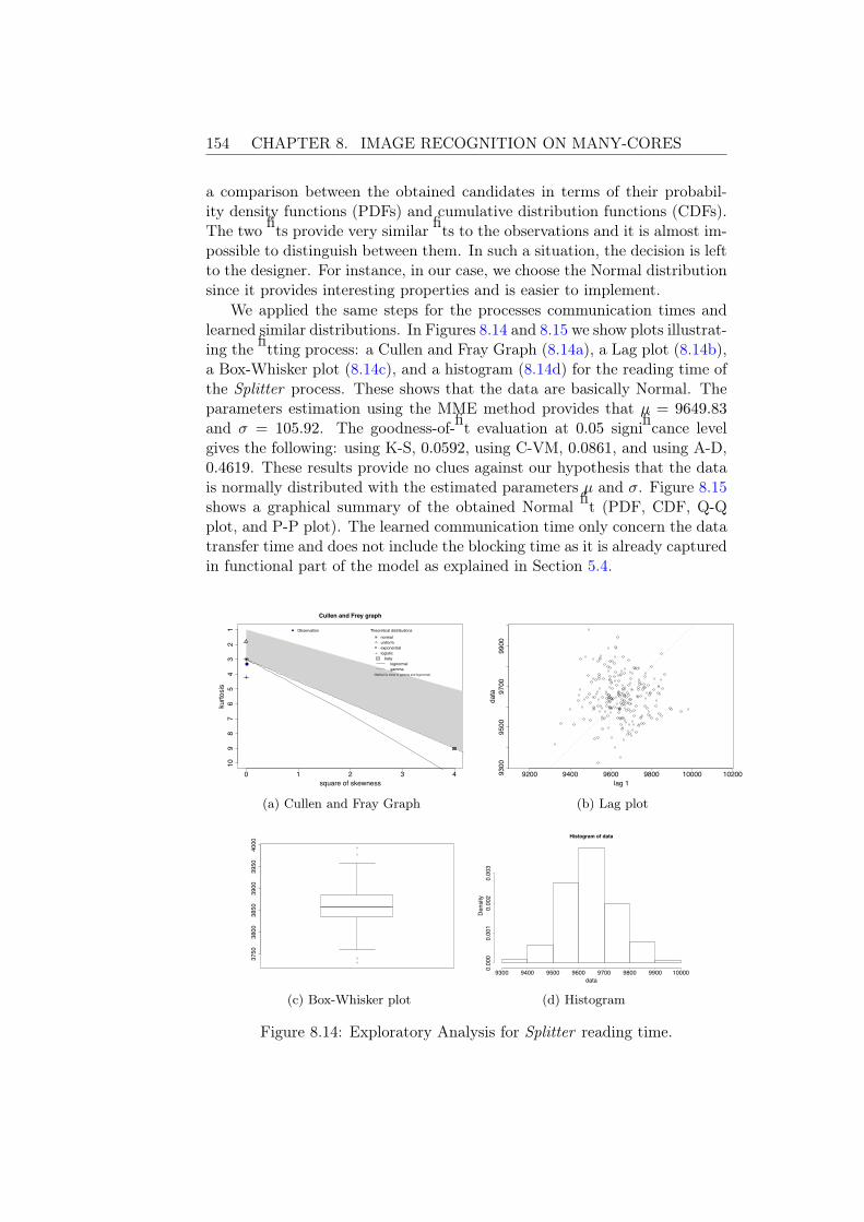
154 CHAPTER 8. IMAGE RECOGNITION ON MANY-CORES
a comparison between the obtained candidates in terms of their probabil-ity density functions (PDFs) and cumulative distribution functions (CDFs).The two fits provide very similar fits to the observations and it is almost im-possible to distinguish between them. In such a situation, the decision is leftto the designer. For instance, in our case, we choose the Normal distributionsince it provides interesting properties and is easier to implement.
We applied the same steps for the processes communication times andlearned similar distributions. In Figures 8.14 and 8.15 we show plots illustrat-ing the fitting process: a Cullen and Fray Graph (8.14a), a Lag plot (8.14b),a Box-Whisker plot (8.14c), and a histogram (8.14d) for the reading time ofthe Splitter process. These shows that the data are basically Normal. Theparameters estimation using the MME method provides that µ = 9649.83and σ = 105.92. The goodness-of-fit evaluation at 0.05 significance levelgives the following: using K-S, 0.0592, using C-VM, 0.0861, and using A-D,0.4619. These results provide no clues against our hypothesis that the datais normally distributed with the estimated parameters µ and σ. Figure 8.15shows a graphical summary of the obtained Normal fit (PDF, CDF, Q-Qplot, and P-P plot). The learned communication time only concern the datatransfer time and does not include the blocking time as it is already capturedin functional part of the model as explained in Section 5.4.
0 1 2 3 4
Cullen and Frey graph
square of skewness
ku
rto
sis
10
98
76
54
32
1 Observation Theoretical distributions
normal
uniform
exponential
logistic
beta
lognormal
gamma
(Weibull is close to gamma and lognormal)
(a) Cullen and Fray Graph
9200 9400 9600 9800 10000 1020093
00
95
00
97
00
99
00
lag 1
da
ta
(b) Lag plot
3750
3800
3850
3900
3950
4000
(c) Box-Whisker plot
Histogram of data
data
Density
9300 9400 9500 9600 9700 9800 9900 10000
0.000
0.001
0.002
0.003
(d) Histogram
Figure 8.14: Exploratory Analysis for Splitter reading time.

CHAPTER 8. IMAGE RECOGNITION ON MANY-CORES 155
Empirical and theoretical dens.
Data
De
nsity
9300 9500 9700 99000.0
00
0.0
02
9400 9600 980093
00
96
00
99
00
Q-Q plot
Theoretical quantiles
Em
pir
ica
l qu
an
tile
s
9300 9500 9700 9900
0.0
0.4
0.8
Empirical and theoretical CDFs
Data
CD
F
0.0 0.2 0.4 0.6 0.8 1.0
0.0
0.4
0.8
P-P plot
Theoretical probabilities
Em
pir
ica
l pro
ba
bili
ties
Figure 8.15: Normal Fit Summary for Splitter reading time.
It is worthwhile mentioning that, in this case study, only the Gabor pro-cess computation time, that is, the compute_filter function was consideredsince we observed that it is the most time consuming. For the other pro-cesses (Splitter and Joiner), only the communication time was character-ized. These are actually doing very light computation consisting of cuttingand assembling data. We also draw the reader attention to the fact thatthe learning of the computation time behavior of the Gabor process is per-formed only for one process. Since all the running Gabors in the system areinstances of the same component which run the same compute_filter func-tion and execute on identical cores, it is safe to calibrate them with the sameprobability distribution. This actually an advantage of using probabilisticcharacterization.
Once all the performance aspects of interest are characterized (in thiscase, we recall that we only consider time), calibration is performed by anno-tating the functional BIP model using the learned distributions as illustratedin Chapter 5. Figure 8.16 shows an example of calibrated BIP component.This corresponds to the Gabor process in Figure 8.6, which is augmentedwith timing information that concerns communication, i.e read and writetime, and the computation time of the compute_filter function, which rep-resents the core computation part of the process. Three different probabilitydistributions where learned to this end, namely µr for the read time, µw forthe writing time, and µc for the computation time. Note that the calibrationphase implies also to modify the FIFO components, as we did in Chapter 5,that is, by decomposing the push and pop actions into begin and end.

156 CHAPTER 8. IMAGE RECOGNITION ON MANY-CORES
[steps == 0]
status = CONFIG
[status==EXEC]
begin_read_data
read(DATA_FIFO_IN, &data)
end_read_data
[time==0]
[steps != 0]
[time>0]
ticktime−−
[time==0]
[time>0]ticktime−−
[time==0]
end_write_data
begin_read_data
data
end_read_data
compute_filter(&data)
data
begin_write_data
write(DATA_FIFO_OUT, data)
[time>0]
tick
time−−steps−−
ticktime−−
status = CONFIG
begin_write_dataend_write_data
read(CONF_FIFO, &config)
steps = config.steps
status = EXEC
[status == CONFIG]
read_conf
read_conf
config
time
tick
l1
l̂3l4
tc ∼ µc
tr ∼ µr
tw ∼ µw
time = trl̂1
l3
tr�
tc�time = tc
tw�time = tw
time = ∞
l0 l2
Figure 8.16: The calibrated model of the Gabor process. An SBIP modelthat represents a part of the obtained performance model of the designedsystem.
8.5 Performance Evaluation
Before using SMC to check the system-level timing requirements, wewanted to validate the calibrated model with respect to the actual imple-mentation. To this end, we compared the overall execution time obtainedby 1) running the generated HMAX implementation on the test-board and2) simulating the calibrated SBIP model. We observed that the time on themodel is about 20% lower than what we obtained on the test-board. Thisresult is expected since the calibrated model does not take into account allthe implementation delays. For instance, the splitting and joining time werenot introduced in the model. Moreover, high-level models are generally moreoptimistic due to abstraction.
Now that we built a high-level performance model that encompasses thefunctional behavior and which is calibrated with timing information, it canbe used for performance evaluation using SMC. We recall that the obtainedmodel is an SBIP model where non-determinism is resolved using prioritieson one hand, and uniform schedulers on the other (see Chapter 3 for moredetails). We use the SPRT algorithm implemented within The BIPSMC
statistical model checker with confidence parameters α = β = 0.001 andδ = 0.05. We checked the aforementioned performance requirements, i.e.,φ1 = Gl(t < Δ) and φ2 = Gl(|tl| < Ψ), for different pipelining rate P ∈{0, 2}. For this case study, we have used arbitrary FIFOs sizes as follows:Main-Splitter= 10 KB, Splitter-Worker= 112 B, Worker-Joiner= 336 B,and Joiner-Main= 30 KB. Note that such a choice might be also exploredusing our approach.

CHAPTER 8. IMAGE RECOGNITION ON MANY-CORES 157
Δ (ms) 572.75 572.79 572.8 572.83 572.85 572.87 572.89 572.91 572.95
P (φ1) 0 0.2 0.28 0.57 0.75 0.91 0.98 0.99 1
Traces 66 457 1513 1110 488 954 171 89 66
Table 8.2: P (φ1) and number of used SMC traces when varying Δ (P = 0).
Table 8.2 shows the probability evolution of φ1 for different Δ and thecorresponding required SMC traces. This first analysis is performed with nopipelining, i.e., P = 0. One can for instance conclude out of this table thatthe overall execution time is always lower than 572.95ms with probability 1.What would be interesting to verify is for instance a trade-off between theobtained timing bound and the used resources in terms of memory utilization.That is, when decreasing the FIFOs sizes, how the overall execution time isimpacted? This is an ongoing work for the moment.
In Figure 8.17, Tables 8.3 and 8.4, we present two results of verifyingφ2 when varying the bound Ψ . The curve on 8.17a is obtained with nopipelining, i.e., (P = 0), while the one on 8.17b is obtained with P =2. The two curves have similar evolution with a small difference in thebounds. The second curve (P = 2) has actually greater values, which reflectmore variation. We recall that when P = 0, all the processes are perfectlysynchronized which yields to small variation over line processing time. UsingP > 0 leads to greater variation since it somehow alter this synchronization.We finally mention that the SMC time was relatively small given the modelsize: 5 hours in average for each property. The BIP model has 47 BIPcomponents and ∼ 6000 lines of code. Components have in average 20control locations and 10 integer variables each, which induces a big statespace.
Ψ (µs) 2095 2100 2110 2115 2120 2125 2130
P (φ2) 0 0.1 0.24 0.47 0.76 0.94 1
Traces 66 65 255 1036 2371 410 66
Table 8.3: P (φ2) and number of used SMC traces when varying Ψ (P = 0).
Ψ (µs) 2280 2285 2290 2300 2305 2310 2315 2320
P (φ2) 0 0.1 0.14 0.64 0.89 0.98 0.99 1
Traces 66 418 394 752 853 206 65 66
Table 8.4: P (φ2) and number of used SMC traces when varying Ψ (P = 2).
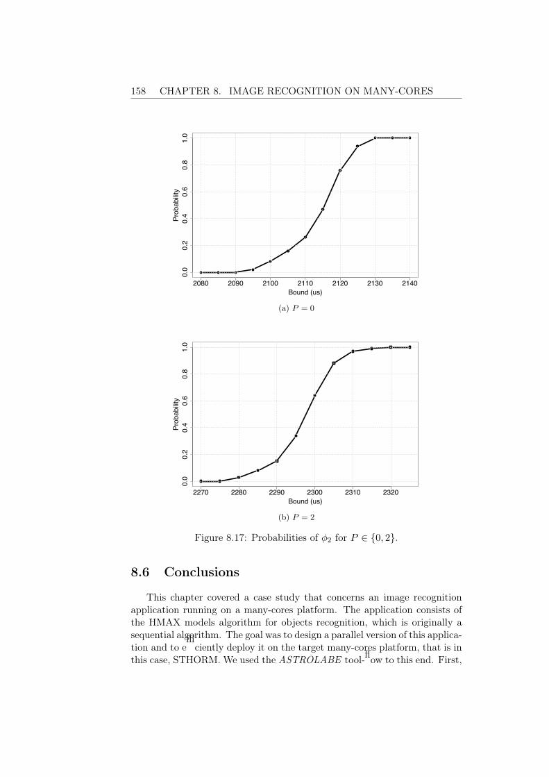
158 CHAPTER 8. IMAGE RECOGNITION ON MANY-CORES
2080 2090 2100 2110 2120 2130 2140
0.0
0.2
0.4
0.6
0.8
1.0
Bound (us)
Pro
ba
bili
ty
(a) P = 0
2270 2280 2290 2300 2310 2320
0.0
0.2
0.4
0.6
0.8
1.0
Bound (us)
Pro
ba
bili
ty
(b) P = 2
Figure 8.17: Probabilities of φ2 for P ∈ {0, 2}.
8.6 Conclusions
This chapter covered a case study that concerns an image recognitionapplication running on a many-cores platform. The application consists ofthe HMAX models algorithm for objects recognition, which is originally asequential algorithm. The goal was to design a parallel version of this applica-tion and to efficiently deploy it on the target many-cores platform, that is inthis case, STHORM. We used the ASTROLABE tool-flow to this end. First,

CHAPTER 8. IMAGE RECOGNITION ON MANY-CORES 159
we built a KPN model of the application following a join/split schema. Usingthe DOL2BIP tool, we obtained a functional BIP model, which was used togenerate a distributed implementation of the application and to deploy it onSTHORM given a certain mapping. We then performed statistical learningto characterize timing information and to derive a performance model, whichwas finally analyzed using SMC against the timing requirements.
Due to time and technical issues, we were not able to explore severalaspects of the system. Actually, the STHORM project was unfortunatelyshut-down by STMicroelectronics and we were only able to experiment on atest-board provided by CEA for limited use. We hence performed only timinganalysis for a single mapping and on a sub-part of the system. What wouldbe interesting is to explore the full version, that is, processing all the inputimage scales and to analyze trade-offs between time and memory, especiallybecause memory is scarce on the fabric side of the platform. Explorationcould also cover several mappings and various images allocation settings. Apreliminary work in this direction can be found in a technical report [164].It is worth mentioning that for this study, we did not use the abstractiontechnique introduced in Chapter 4, since the obtained performance modelwas affordable using bare SMC algorithms.


Chapter 9Conclusions and Perspectives
Conclusions
The main objective of the present work is to enable better support ofperformance aspects in system-level design of many-core embedded systems.As exposed along the manuscript, our belief is that such support can only bepossible within a holistic and rigorous approach that provides systematic andtool-supported steps performed in an iterative and incremental fashion. Ourgoal was thus to conceive an approach that follows these guide-lines and thateventually leads to a correct and efficient implementation of a given system.To precisely identify how to handle performance at system-level, we analyzedthe existing and sought challenges in this area. We were able to identifymodeling and analysis as essential activities and to specify requirements thatmust be satisfied to answer the identified challenges.
We proposed the SBIP stochastic component-based modeling languageand its associated formal semantics as answer to rigorousness, incrementality,and expressiveness requirements. The proposed modeling language is seen asthe spine of the conceived approach. It enables to capture different aspects ofembedded systems, especially performance and induced variability, throughthe proposed stochastic semantics that allows for modeling probabilistic andnon-deterministic behaviors, i.e., MDPs. Designing following a component-based fashion enables natural thinking and building of systems and helpsmastering complexity. Furthermore, formal semantics allows for rigorousand automated reasoning about the designed system.
On top of the SBIP formalism, we built a probabilistic model checker,namely BIPSMC , in order to perform quantitative analysis, which is ofparamount importance for performance evaluation. This tool uses a mixof simulation and statistical-based approaches, which provide a good trade-off between accuracy, rapidity, and scalablity requirements. We presentedan example of using the SBIP formalism and the BIPSMC tool for verifying
161
162 CHAPTER 9. CONCLUSIONS AND PERSPECTIVES
a multimedia system. As for any formal analysis technique, SMC suffersfrom state space explosion issues. To bypass this hindrance, we proposedan abstraction technique that computes a smaller stochastic model given acertain requirement. The suggested technique uses projection with respectto a given property to keep only the relevant behavior of the system, andmachine learning to build a compact representation. The method was shownto converge in the limit to a small yet accurate representation of the originalsystem.
The above contributions, which were presented in the first part of themanuscript, besides being an important part of the theoretical foundation ofthe proposed performance modeling and analysis approach, they representa generic and a formal framework for rigorous modeling and quantitativeanalysis of stochastic systems. They may be used in a different context thanperformance modeling and analysis at system-level. This is the reason wechoose to present them in a separate part.
An important challenge that was identified during the analysis of require-ments for system-level performance modeling is to figure out the appropriatelevel of abstraction of the system model to build. To produce a trustwor-thy design, such models must capture a sufficient amount of information thatconcern functional and performance aspects of the system, that is, they mustbe faithful. Given this requirement, we conceived a modeling approach thataims at producing performance models offering good trade-offs between thelevel of abstraction and the degree of faithfulness required in early designphases. The proposed method follows a meet-in-the-middle scheme and iscomposed of three main tasks, namely, code generation, distribution fitting,and models calibration. The idea of the approach is to combine behavioralinformation coming from high-level functional models and low-level perfor-mance details obtained from real executions or low-level simulations.
In spite of being part of the performance modeling approach, the codegeneration contribution answers the requirement of quickly programming andsoftware prototyping on many-cores platforms. The goal of this task is togenerate a distributed implementations and the associated deployment of agiven high-level functional model on a target many-cores platform. Such im-plementation allows for concrete executions and thus for observing real per-formance evolution, which is enabled through code instrumentation with re-spect to the performance dimension of interest. In order to faithfully capturesuch information and to characterize it, we opted for probabilistic modelingwhich enables to capture performance fluctuations and allows for operatingnatural abstraction of irrelevant details. To this end, we used a statisticalinference process, more precisely distribution fitting, which consists of learn-ing the best probability distribution that characterizes the performance data.Finally, we combine the high-level functional behavior with the probabilis-tic performance characterization to obtain a stochastic performance modelusing a model calibration step. Calibration consists of injecting the learned

CHAPTER 9. CONCLUSIONS AND PERSPECTIVES 163
probability distributions within the functional model by introducing prob-abilistic variables and time progress in the case of timing performance forinstance.
All the above steps compose the ASTROLABE integrated approach weproposed for performance modeling and analysis at system-level. In thisapproach, performance modeling relies on the steps above and the obtainedperformance model is analyzed with respect to performance requirements us-ing the stochastic abstraction and the statistical model checking techniques.We also depicted a tool-flow covering most of the steps of the ASTROLABEapproach, e.g., DistFit tool for distribution fitting and BIP2MCAPI codegenerator for the STHORM many-core platform and the MCAPI runtime.The approach and its associated tool-flow was illustrated on a fragment ofa real-life case study for image recognition. The initial results of this studywere encouraging and showed that good performance models can be ob-tained quickly and easily from high-level specifications. Moreover, analysisusing statistical model checking provided quick and accurate results. Anal-ysis is for now done only for timing aspects and we are planning to extendit for further performance dimensions as stated in the perspective sectionhereafter.
Perspectives
In the above contributions, several amelioration and extensions are soughtto enable covering additional aspects and hence ensure more generality forthe proposed approach for system-level performance modeling and analysis.
The SBIP Extension
The SBIP formalism can be extended at different levels. First, with re-spect to time granularity. As presented in Chapter 3, the proposed semanticsonly covers discrete-time, i.e., MDPs and LMCs. It would be interesting toextend this semantics to cover in addition continuous time. Such extensionwould help to build models that capture timing aspects more naturally. Forinstance, when calibrating functional models with probability distributionscharacterizing computation or communication time, one can think of addingstochastic clocks that evolve continuously with respect to the learned prob-ability distributions, instead of adding probabilistic variables and modelingtime evolution via discrete transitions. To do so, we may rely on the real-timesemantics of the BIP formalism [1] where time is a first-class concept, thatis, a full-fledged part of the semantics. In contrast, to the BIP semantics, inreal-time BIP, time is not explicitly simulated using discrete transitions, e.g.,tick, but is implicitly handled by an engine that implements the real-timesemantics.

164 CHAPTER 9. CONCLUSIONS AND PERSPECTIVES
Considering stochastic clocks is not trivial, especially in a component-based formalism because of the induced complexity of parallel compositionof components. Various works have proposed models combining time andstochastic behavior such as Stochastic Petri nets [4], stochastic process al-gebra [112, 114], stochastic automata [71, 72], stochastic timed automata[70, 36] used for instance in MoDest, and priced timed automata used in Up-paal [74]. These models often have CTMCs or more general GSMPs [98, 7]semantics.
A second amelioration in SBIP may cover the probabilistic schedulers,which are currently limited to uniform distributions. As stated in Chapter 3,this is the default choice we made for simplicity of implementation. Allow-ing additional probability distributions for schedulers, implies to extend theSBIP modeling language. This can be done for instance using weights addedon interactions or on the ports of the components. Given a set of enabledinteractions at some point, a normalization is then performed in order tocompute the underlying probabilities and to accordingly select the interac-tion to fire. We may also extend the proposed formalism with a rewardsemantics. This will be useful when considering other performance aspectssuch as energy and temperature. We believe that such extension is straight-forward if we use SBIP variables and associate them with reward functions.This is for instance the case in Uppaal [74] and Prism [139].
Stochastic Abstraction
In the present work, we used the AAlergia algorithm to instantiate ourapproach for automatically building sound abstractions. We recall that theapproach is limited to bounded LTL properties when using algorithms onlyable to learn deterministic models such as AAlergia, and when the used datacontains non-determinism. This represents a hindrance towards checkingunbounded properties using probabilistic model checking for instance, espe-cially that the proposed projection potentially introduces non-determinismin the data. We may use other algorithms able to learn non-deterministicmodels, such as 1 [194, 193, 154, 180] to remedy to this issue. However, werecall that when learning non-deterministic models, it is only possible tocompute upper and lower probability bounds for various schedulers requiredto resolve non-determinism.
With respect to the projection part, there are also possibilities of im-provement. The current projection definition enables building abstractionfor classes of properties since it considers the support of a given property asthe set of its explicitly appearing symbols. We may for example take intoaccount the semantics of LTL operators to define coarser projections and ob-tain consequently more compact abstractions, albeit this has the limitation
1. Additional work are presented in the related work section in Chapter 4.

CHAPTER 9. CONCLUSIONS AND PERSPECTIVES 165
of recalculating a new abstraction for each single property.
Remark that the models obtained by using our abstraction techniqueare LMCs or MDPs. These may be easily transformed into SBIP modelsas shown in Section 3.4. However, the proposed transformation capturesthe given model as a single SBIP component, that is, we loose composi-tionality. It would be interesting to learn SBIP models in a compositionalfashion, that is, models having different interacting components. Such ap-proach would require in addition to learn connections or a glue between theobtained components, which is a challenging task. Some work has been donein this direction within the BIP framework [25, 27, 26, 39], although still in apreliminary state. This approach may be directly integrated within a learn-ing algorithm, which is quite difficult, or performed post learning, that is,once an LMC or MDP model is obtained.
Statistical Inference
The statistical inference procedure described in Chapter 6 is anotherlearning technique that aims at inferring probabilistic models from inputdata. In the present work, we used distribution fitting as to learn probabilitydistributions. A more general approach is model fitting that fits an arbitrarymodel to the data. In the case of distribution fitting, the target model canbe only a probability distribution and obey to some assumptions such asdata independence as discussed in Chapter 6. A well known family of modelfitting techniques is regression analysis [8, 96, 175, 3]. Techniques as suchARMA and ARIMA can be used to characterize the behavior of a certainrandom variable as a linear or non-linear function of a single or several othervariables.
A learned lesson from the case study we performed in this work is thatstatistical inference techniques require human expertise and intervention.Various activities in such process rely on human interpretation and are thusdifficult to automate, such as the exploratory analysis phase in the proposeddistribution fitting approach. A possible fully automated procedure mayrely on machine learning. In the related work section in Chapter 4, wediscussed several algorithms that are able to learn probabilistic and timedmodels for instance. These may be appropriate to characterize in moredetail timing aspects of embedded systems. Consequently, they may be usedin advanced phases of the design to learn more detailed description. Suchalgorithms produce Markov models and not probability distributions. Thus,model calibration will consist of transforming the learned model to an SBIPcomponent and to inject it in the functional model, which requires to addextra connectors for synchronization.

166 CHAPTER 9. CONCLUSIONS AND PERSPECTIVES
The ASTROLABE Approach
At the level of the proposed ASTROLABE approach, we suggest ad-ditional future directions. The proposed approach provides quantitativeanalysis results with respect to performance requirements. However, suchfeed-backs do not explicitly guide the designer to improve or modify specificparts of the input models or mapping. In design space exploration, the idea isto keep, at each design phase, configurations ensuring functional correctnessand good trade-offs between the explored performance aspects. Coming-upwith different design alternatives is a separate matter which is more relatedto human expertise.
Design trade-offs may be obtained by exploring the space of quantitativefeed-backs that concern the performance dimensions of interest, e.g., timing,memory utilization, energy consumption. Exploration can be performedmanually [92], or using exhaustive [215] or randomized [49, 9] search forinstance. Additional possibilities exist such as the reduction to a singleobjective [57] or problem-dependent approaches [195] (see [136, 31] for adetailed classifications and discussion). These exploration techniques rely ondifferent search and optimization algorithms often multi-objective since theyconcern various aspects of the systems, which are generally contradictoryand of different nature. A well known technique that enables comparison ofsuch heterogeneous aspects is Pareto Dominance, which allows for a partialordering. Example of approaches used for design space exploration rely ongenetic algorithms [48], multi-objective optimization [174, 122], dependency[97] and Pareto sensitivity [90] analysis techniques.
We recall that in our work, we rely on statistical model checking to quan-titatively evaluate design alternatives with respect to performance require-ments. Such evaluation is based on verifying formal properties expressed inLTL for example. We can formalize properties that cover the different per-formance dimensions as a conjunction of several aspects. Consequently, oneobtains a single probability measure, that quantify the different performancedimensions, per configuration. Now for different configurations it is easier topick the highest probability.
Note that in the current state of the work we only cover one performancedimension, that is, timing. The reason for this limitation is the distributionfitting approach and the strong assumption of data independence. If weextend our statistical inference technique as discussed in the previous section,it is possible to handle other dimensions such as energy and temperature,which often expose dependencies.
Technical Improvements
In addition to the above improvement, we may think of technical en-hancement for the tool-flow we implemented. For instance, the BIPSMC

CHAPTER 9. CONCLUSIONS AND PERSPECTIVES 167
tool may benefit from a graphical interface instead of command-line. Sev-eral optimization may be also operated, such as the properties monitoringalgorithm, in addition to the possible extension of the property specificationlanguage to cover nested operators, which requires systematic procedure forgenerating more complex monitors. It is also worth continuing the explo-ration of the image processing case study with respect to trade-offs betweentime and memory utilization and to consider the full S1 layer to challengethe statistical model checking technique we are using for analysis. This mayrequire using the abstraction technique for instance as the obtained modelmight be too big. The instrumentation of the generated code to get per-formance data can be automated through the use of special annotations.The latter could be introduced at the level of the functional BIP model anddeduced from the performance properties under consideration. Later, whenperforming code generation the introduced annotations may be transformedto specific functions calls, given the target runtime and platform support.We can also automate the calibration process, at least for timing information,following the rules defined in Chapter 5.


List of Figures
1.1 The Y-chart Scheme for mapping application to architecture. 61.2 Schematic view of exploring the design space. . . . . . . . . . 71.3 A generic process of design space exploration. . . . . . . . . . 81.4 Building separate purely functional and performance models. 151.5 Illustration of the model checking verification method. . . . . 191.6 Overview of the ASTROLABE method. . . . . . . . . . . . . 22
2.1 An LMC model for the Craps Gambling Game. . . . . . . . . 292.2 An MDP example. . . . . . . . . . . . . . . . . . . . . . . . . 302.3 Markov chain induced by scheduler S on the MDP of Figure 2.2. 32
3.1 An example of a BIP atomic component. . . . . . . . . . . . . 433.2 A BIP component of a processing unit of a video decoding
system. . . . . . . . . . . . . . . . . . . . . . . . . . . . . . . 453.3 BIP example: Sender-Buffer-Receiver system. . . . . . . . . . 473.4 Priority restriction example. . . . . . . . . . . . . . . . . . . . 483.5 Behavior of the System component in Figure 3.3. . . . . . . . 493.6 Example of a stochastic atomic component Bs and its behavior. 513.7 Example of a stochastic atomic component Bs and associated
MDP. . . . . . . . . . . . . . . . . . . . . . . . . . . . . . . . 543.8 A Stochastic Multimedia Stream Source model. . . . . . . . . 543.9 Illustration of the stochastic semantics of composition in SBIP. 563.10 SBIP component of an MPEG2 Stream Source. . . . . . . . . 583.11 LMC induced by a uniform scheduler S on the MDP Fig-
ure 3.7c. . . . . . . . . . . . . . . . . . . . . . . . . . . . . . . 593.12 An abstract view of a multimedia SoC. . . . . . . . . . . . . . 603.13 Evolution of the play-out buffer fill-level over time. . . . . . . 613.14 Frequency distributions of I,P, and B frames. . . . . . . . . . 623.15 SBIP model of the multimedia SoC. . . . . . . . . . . . . . . 623.16 A generic SBIP model of a buffer component. . . . . . . . . . 633.17 SBIP model of the Player component. . . . . . . . . . . . . . 63
169

170 LIST OF FIGURES
3.18 SBIP model of the Observer component. . . . . . . . . . . . . 653.19 Play-out buffer fill-level and probability of φ for cact.m2v. . . 663.20 Play-out buffer fill-level and probability of φ for mobile.m2v. 673.21 Play-out buffer fill-level and probability of φ for tennis.m2v. 673.22 Transformation rules of LMCs to SBIP model. . . . . . . . . 693.23 An example of transformation of an LMC to an SBIP model. 703.24 Behavior of the obtained SBIP component from an LMC. . . 723.25 Transformation rules of MDPs to SBIP model. . . . . . . . . 743.26 An example of transformation of an MDP to an SBIP model. 753.27 Behavior of the obtained SBIP component from an MDP. . . 76
4.1 Main steps of the AAlergia algorithm. . . . . . . . . . . . . . 824.2 Illustration of our approach for learning abstract models. . . . 834.3 Learned abstract models of the Craps Gambling Game. . . . . 864.4 Abstract Herman’s Self Stabilizing Protocol models. . . . . . 894.5 Statistical Model Checking Time of ϕ10 using PESTIM. . . . 914.6 ϕL verification results using PESTIM for M = {7, 11}. . . . . 914.7 ϕL verification results using PESTIM for M = {19, 21}. . . . 924.8 Abstract Herman’s Self Stabilizing Protocol model with M =
7 for φ. . . . . . . . . . . . . . . . . . . . . . . . . . . . . . . 93
5.1 The ASTROLABE approach. . . . . . . . . . . . . . . . . . . 1025.2 Memory access and arbitration mechanism. . . . . . . . . . . 1065.3 Impact of arbitration mechanism on execution time. . . . . . 1075.4 Calibration of functional models with computation time. . . . 1095.5 Calibration of functional model with communication time. . . 1105.6 Example of communication through a fifo buffer. . . . . . . . 1105.7 Calibration of the functional model in Figure 5.6. . . . . . . . 1115.8 Bad calibration of the functional model in Figure 5.6. . . . . . 112
6.1 Histogram of 500 Normally distributed observations. . . . . . 1186.2 Box-Whisker Plot of 500 Normally distributed observations. . 1186.3 Lag Plot of 500 Normally distributed observations. . . . . . . 1196.4 Fitted Normal distributions obtained using the estimation
methods. . . . . . . . . . . . . . . . . . . . . . . . . . . . . . . 1226.5 Q-Q plot of the different fits. . . . . . . . . . . . . . . . . . . 1226.6 Comparison of the CDFs of the obtained fits. . . . . . . . . . 123
7.1 Illustration of the ASTROLABE tool-flow. . . . . . . . . . . . 1287.2 DistFit Tool: the different steps, inputs, and outputs. . . . . . 1317.3 BIPSMC tool architecture: diagram of the main modules. . . 1327.4 Example of a DTMC model and its specification in SBIP. . . 1347.5 The ASTROLABE tool-flow extended with several tools. . . . 1377.6 A KPN model example consisting of a split/join schema. . . . 1377.7 The BIP model of the Worker example Figure 7.6. . . . . . . 138

LIST OF FIGURES 171
8.1 HMAX models algorithm overview. . . . . . . . . . . . . . . . 1428.2 Example of input and output images of the HMAX S1 layer. . 1438.3 MCAPI domains on STHORM. . . . . . . . . . . . . . . . . . 1448.4 An abstract view of the S1 layer of HMAX models algorithm. 1458.5 The simplified model of the S1 layer of HMAX models algorithm.1478.6 A functional BIP model of the Gabor process. . . . . . . . . . 1478.7 A BIP model of a FIFO buffer. . . . . . . . . . . . . . . . . . 1488.8 Box and Runs plots of the Gabor execution time. . . . . . . . 1498.9 Box and Runs plots of the Gabor execution time without out-
liers. . . . . . . . . . . . . . . . . . . . . . . . . . . . . . . . . 1508.10 Lag plot of the Gabor execution time. . . . . . . . . . . . . . 1508.11 Histogram and CDF of the Gabor execution time observations. 1518.12 Cullen and Frey graph for the Gabor execution time. . . . . . 1528.13 Graphical comparison between the Normal and the Gamma fits.1538.14 Exploratory Analysis for Splitter reading time. . . . . . . . . 1548.15 Normal Fit Summary for Splitter reading time. . . . . . . . . 1558.16 The calibrated model of the Gabor process. . . . . . . . . . . 1568.17 Probabilities of φ2 for P ∈ {0, 2}. . . . . . . . . . . . . . . . . 158


List of Tables
3.1 Summary of the stochastic extension of the BIP formalism. . 60
4.1 Verification results of ϕ1 on Craps: original vs. abstract models 864.2 Summary of the possible settings and the corresponding results. 884.3 Abstraction and verification results of ϕ10 and ψ30 using PES-
TIM. . . . . . . . . . . . . . . . . . . . . . . . . . . . . . . . . 904.4 SMC of ψL
M on the original and the learned Herman’s models. 93
6.1 Results of the goodness-of-fit tests of the obtained fits. . . . . 1256.2 BIC and AIC scores for the obtained fits. . . . . . . . . . . . 125
7.1 MCAPI endpoints memory attributes. . . . . . . . . . . . . . 129
8.1 GOF evaluation results for the Normal and Gamma fits. . . . 1528.2 P (φ1) and number of used SMC traces when varying Δ (P = 0).1578.3 P (φ2) and number of used SMC traces when varying Ψ (P = 0).1578.4 P (φ2) and number of used SMC traces when varying Ψ (P = 2).157
173


Bibliography
[1] Tesnim Abdellatif, Jacques Combaz, and Joseph Sifakis. Rigorous im-plementation of real-time systems–from theory to application. Mathe-matical Structures in Computer Science, 23(04):882–914, 2013.
[2] Gul Agha, José Meseguer, and Koushik Sen. Pmaude: Rewrite-based specification language for probabilistic object systems. Elec-tronic Notes in Theoretical Computer Science, 153(2):213–239, 2006.
[3] Sumit Ahuja, Deepak A Mathaikutty, Avinash Lakshminarayana, andSandeep K Shukla. Scope: Statistical regression based power modelsfor co-processors power estimation. Journal of Low Power Electronics,5(4):407–415, 2009.
[4] Marco Ajmone Marsan, Gianni Conte, and Gianfranco Balbo. A classof generalized stochastic petri nets for the performance evaluationof multiprocessor systems. ACM Transactions on Computer Systems(TOCS), 2(2):93–122, 1984.
[5] Husain Aljazzar, Manuel Fischer, Lars Grunske, Matthias Kuntz, Flo-rian Leitner-Fischer, and Stefan Leue. Safety analysis of an airbagsystem using probabilistic fmea and probabilistic counterexamples. InQuantitative Evaluation of Systems, 2009. QEST’09. Sixth Interna-tional Conference on the, pages 299–308. IEEE, 2009.
[6] Musab AlTurki and José Meseguer. Pvesta: A parallel statistical modelchecking and quantitative analysis tool. In CALCO, pages 386–392,2011.
[7] Rajeev Alur, Costas Courcoubetis, and David Dill. Model-checkingfor probabilistic real-time systems. In Automata, Languages and Pro-gramming, pages 115–126. Springer, 1991.
[8] Theodore Wilbur Anderson. The new statistical analysis of data.Springer, 1996.
[9] Urs Anliker, Jan Beutel, Matthias Dyer, Rolf Enzler, Paul Lukowicz,Lothar Thiele, and Gerhard Troster. A systematic approach to the
175

176 BIBLIOGRAPHY
design of distributed wearable systems. Computers, IEEE Transactionson, 53(8):1017–1033, 2004.
[10] Lacramioara Aştefănoaei, Souha Ben Rayana, Saddek Bensalem, Mar-ius Bozga, and Jacques Combaz. Compositional invariant generationfor timed systems. In Tools and Algorithms for the Construction andAnalysis of Systems, pages 263–278. Springer, 2014.
[11] Adnan Aziz, Kumud Sanwal, Vigyan Singhal, and Robert Brayton.Model-checking continuous-time markov chains. ACM Transactionson Computational Logic (TOCL), 1(1):162–170, 2000.
[12] Adnan Aziz, Vigyan Singhal, Felice Balarin, Robert K Brayton, andAlberto L Sangiovanni-Vincentelli. It usually works: The temporallogic of stochastic systems. In Computer Aided Verification, pages155–165. Springer, 1995.
[13] Christel Baier, Nathalie Bertrand, Patricia Bouyer, Thomas Brihaye,and M Grosser. Almost-sure model checking of infinite paths in one-clock timed automata. In Logic in Computer Science, 2008. LICS’08.23rd Annual IEEE Symposium on, pages 217–226. IEEE, 2008.
[14] Christel Baier, Edmund M Clarke, Vasiliki Hartonas-Garmhausen,Marta Kwiatkowska, and Mark Ryan. Symbolic model checking forprobabilistic processes. Springer, 1997.
[15] Christel Baier and Joost-Pieter Katoen. Principles of model checking.MIT Press, 2008.
[16] Amol Bakshi, Viktor K Prasanna, and Akos Ledeczi. Milan: A modelbased integrated simulation framework for design of embedded sys-tems. ACM Sigplan Notices, 36(8):82–93, 2001.
[17] Felice Balarin. Hardware-software co-design of embedded systems: thePOLIS approach. Springer, 1997.
[18] Felice Balarin, Yosinori Watanabe, Harry Hsieh, Luciano Lavagno,Claudio Passerone, and Alberto Sangiovanni-Vincentelli. Metropo-lis: An integrated electronic system design environment. Computer,36(4):45–52, 2003.
[19] Paolo Ballarini, Hilal Djafri, Marie Duflot, Serge Haddad, and NihalPekergin. Cosmos: a statistical model checker for the hybrid automatastochastic logic. In Quantitative Evaluation of Systems (QEST), 2011Eighth International Conference on, pages 143–144. IEEE, 2011.
[20] Paolo Ballarini, Hilal Djafri, Marie Duflot, Serge Haddad, and NihalPekergin. Hasl: an expressive language for statistical verification ofstochastic models. In Proceedings of the 5th International ICST Con-ference on Performance Evaluation Methodologies and Tools, pages306–315. ICST (Institute for Computer Sciences, Social-Informaticsand Telecommunications Engineering), 2011.

BIBLIOGRAPHY 177
[21] Benoît Barbot, Serge Haddad, and Claudine Picaronny. Coupling andimportance sampling for statistical model checking. In Tools and Algo-rithms for the Construction and Analysis of Systems, pages 331–346.Springer, 2012.
[22] Ananda Basu, Saddek Bensalem, Marius Bozga, Paraskevas Bourgos,Mayur Maheshwari, and Joseph Sifakis. Component assemblies in thecontext of manycore. In FMCO, pages 314–333, 2011.
[23] Ananda Basu, Saddek Bensalem, Marius Bozga, Paraskevas Bourgos,Mayur Maheshwari, and Joseph Sifakis. Component assemblies in thecontext of manycore. In Formal Methods for Components and Objects,pages 314–333. Springer, 2013.
[24] Ananda Basu, Saddek Bensalem, Marius Bozga, Paraskevas Bourgos,and Joseph Sifakis. Rigorous system design: the bip approach. InMathematical and Engineering Methods in Computer Science, pages1–19. Springer, 2012.
[25] Ananda Basu, Saddek Bensalem, Marius Bozga, Benoît Caillaud,Benoît Delahaye, and Axel Legay. Statistical abstraction and model-checking of large heterogeneous systems. In Formal Techniques forDistributed Systems, pages 32–46. Springer, 2010.
[26] Ananda Basu, Saddek Bensalem, Marius Bozga, Benoît Delahaye, andAxel Legay. Statistical abstraction and model-checking of large het-erogeneous systems. STTT, 14(1):53–72, 2012.
[27] Ananda Basu, Saddek Bensalem, Marius Bozga, Benoît Delahaye, AxelLegay, and Emmanuel Sifakis. Verification of an afdx infrastructureusing simulations and probabilities. In RV, pages 330–344, 2010.
[28] Ananda Basu, Marius Bozga, and Joseph Sifakis. Modeling heteroge-neous real-time components in bip. In SEFM, pages 3–12, 2006.
[29] Ananda Basu, Matthieu Gallien, Charles Lesire, Thanh-Hung Nguyen,Saddek Bensalem, Félix Ingrand, and Joseph Sifakis. Incrementalcomponent-based construction and verification of a robotic system.In ECAI, volume 178, pages 631–635, 2008.
[30] Gerd Behrmann, Alexandre David, and Kim G Larsen. A tutorial onuppaal. In Formal methods for the design of real-time systems, pages200–236. Springer, 2004.
[31] Meena Belwal and TSB Sudarshan. A survey on design space explo-ration for heterogeneous multi-core. In Embedded Systems (ICES),2014 International Conference on, pages 80–85. IEEE, 2014.
[32] Saddek Bensalem, Marius Bozga, Benoît Delahaye, Cyrille Jégourel,Axel Legay, and Ayoub Nouri. Statistical model checking qos propertiesof systems with sbip. In ISoLA (1), pages 327–341, 2012.

178 BIBLIOGRAPHY
[33] Saddek Bensalem, Marius Bozga, Thanh-Hung Nguyen, and JosephSifakis. D-finder: A tool for compositional deadlock detection andverification. In CAV, pages 614–619, 2009.
[34] Saddek Bensalem, Andreas Griesmayer, Axel Legay, Thanh-HungNguyen, Joseph Sifakis, and Rongjie Yan. D-finder 2: Towards ef-ficient correctness of incremental design. In NASA Formal Methods,pages 453–458. Springer, 2011.
[35] Saddek Bensalem, Axel Legay, Ayoub Nouri, and Doron Peled.Synthesizing distributed scheduling implementation for probabilisticcomponent-based systems. In MEMOCODE, pages 87–96, 2013.
[36] Nathalie Bertrand, Patricia Bouyer, Thomas Brihaye, Quentin Menet,Christel Baier, Marcus Groesser, and Marcin Jurdzinski. Stochastictimed automata. arXiv preprint arXiv:1410.2128, 2014.
[37] Simon Bliudze and Joseph Sifakis. The algebra of connectors - struc-turing interaction in bip. IEEE Trans. Computers, 57(10):1315–1330,2008.
[38] Simon Bliudze and Joseph Sifakis. A notion of glue expressiveness forcomponent-based systems. In CONCUR 2008-Concurrency Theory,pages 508–522. Springer, 2008.
[39] Simon Bliudze and Joseph Sifakis. Synthesizing glue operators fromglue constraints for the construction of component-based systems. InSoftware Composition, pages 51–67. Springer, 2011.
[40] Alex Bobrek, Joshua J Pieper, Jeffrey E Nelson, JoAnn M Paul, andDonald E Thomas. Modeling shared resource contention using a hybridsimulation/analytical approach. In Design, Automation and Test inEurope Conference and Exhibition, 2004. Proceedings, volume 2, pages1144–1149. IEEE, 2004.
[41] Jonathan Bogdoll, Luis María Ferrer Fioriti, Arnd Hartmanns, andHolger Hermanns. Partial order methods for statistical model checkingand simulation. In Formal Techniques for Distributed Systems, pages59–74. Springer, 2011.
[42] Borzoo Bonakdarpour, Marius Bozga, Mohamad Jaber, Jean Quilbeuf,and Joseph Sifakis. A framework for automated distributed implemen-tation of component-based models. Distributed Computing, 25(5):383–409, 2012.
[43] P Bourgos, A Basu, S Bensalem, K Huang, and J Sifakis. Integratingarchitectural constraints in application software by source-to-sourcetransformation in bip. Technical report, Technical Report TR-2011-1,Verimag Research Report, 2010.
[44] Paraskevas Bourgos. Rigorous Design Flow for Programming ManycorePlatforms. PhD thesis, Univesité de Grenoble, 2013.
BIBLIOGRAPHY 179
[45] Paraskevas Bourgos, Ananda Basu, Marius Bozga, Saddek Bensalem,Joseph Sifakis, and Kai Huang. Rigorous system level modeling andanalysis of mixed hw/sw systems. In MEMOCODE, pages 11–20, 2011.
[46] Patricia Bouyer, Kim G Larsen, and Nicolas Markey. Model-checkingone-clock priced timed automata. In Foundations of Software Scienceand Computational Structures, pages 108–122. Springer, 2007.
[47] George EP Box and David A Pierce. Distribution of residual auto-correlations in autoregressive-integrated moving average time seriesmodels. Journal of the American statistical Association, 65(332):1509–1526, 1970.
[48] Carlo Brandolese, William Fornaciari, Luigi Pomante, Fabio Salice,and Donatella Sciuto. Affinity-driven system design exploration forheterogeneous multiprocessor soc. Computers, IEEE Transactions on,55(5):508–519, 2006.
[49] Davide Bruni, Alessandro Bogliolo, and Luca Benini. Statistical designspace exploration for application-specific unit synthesis. In Design Au-tomation Conference, 2001. Proceedings, pages 641–646. IEEE, 2001.
[50] Peter Bulychev, Alexandre David, Kim G Larsen, Axel Legay, andMarius Mikučionis. Computing nash equilibrium in wireless ad hoc net-works: A simulation-based approach. arXiv preprint arXiv:1202.4506,2012.
[51] Peter E. Bulychev, Alexandre David, Kim Guldstrand Larsen, MariusMikucionis, Danny Bøgsted Poulsen, Axel Legay, and Zheng Wang.Uppaal-smc: Statistical model checking for priced timed automata. InQAPL, pages 1–16, 2012.
[52] Doron Bustan, Sasha Rubin, and Moshe Y Vardi. Verifying ω-regularproperties of markov chains. In Computer Aided Verification, pages189–201. Springer, 2004.
[53] Lukai Cai and Daniel Gajski. Transaction level modeling: an overview.In Proceedings of the 1st IEEE/ACM/IFIP international conference onHardware/software codesign and system synthesis, pages 19–24. ACM,2003.
[54] Rafael C. Carrasco and José Oncina. Learning stochastic regular gram-mars by means of a state merging method. In ICGI, pages 139–152,1994.
[55] Samarjit Chakraborty, Simon Künzli, and Lothar Thiele. A generalframework for analysing system properties in platform-based embed-ded system designs. In DATE, volume 3, page 10190. Citeseer, 2003.
[56] Souymodip Chakraborty, Joost-Pieter Katoen, Falak Sher, and MartinStrelec. Modelling and statistical model checking of a microgrid. In-ternational Journal on Software Tools for Technology Transfer, pages1–18, 2014.

180 BIBLIOGRAPHY
[57] Chantana Chantrapornchai, Edwin H-M Sha, and Xiaobo SharonHu. Efficient design exploration based on module utility selection.Computer-Aided Design of Integrated Circuits and Systems, IEEETransactions on, 19(1):19–29, 2000.
[58] Stavros Tripakis Christopher Brooks, Edward A. Lee. Ptolemy tutorial:Exploring models of computation with ptolemy ii. A tutorial presentedin ESWeek, 2010.
[59] Frank Ciesinski and Marcus Größer. On probabilistic computation treelogic. In Validation of Stochastic Systems, pages 147–188. Springer,2004.
[60] Edmund M Clarke, Alexandre Donzé, and Axel Legay. Statisticalmodel checking of mixed analog circuits. Formal Verification of AnalogCircuits, Workshop of CAV, 2008.
[61] Edmund M Clarke, Alexandre Donzé, and Axel Legay. On simulation-based probabilistic model checking of mixed-analog circuits. FormalMethods in System Design, 36(2):97–113, 2010.
[62] Edmund M Clarke and E Allen Emerson. Design and synthesis of syn-chronization skeletons using branching time temporal logic. Springer,1982.
[63] Edmund M Clarke, James R Faeder, Christopher J Langmead,Leonard A Harris, Sumit Kumar Jha, and Axel Legay. Statisticalmodel checking in biolab: Applications to the automated analysis of t-cell receptor signaling pathway. In Computational Methods in SystemsBiology, pages 231–250. Springer, 2008.
[64] Edmund M Clarke and Paolo Zuliani. Statistical model checking forcyber-physical systems. In Automated Technology for Verification andAnalysis, pages 1–12. Springer, 2011.
[65] Jamieson M Cobleigh, Dimitra Giannakopoulou, and Corina S Păsăre-anu. Learning assumptions for compositional verification. In Toolsand Algorithms for the Construction and Analysis of Systems, pages331–346. Springer, 2003.
[66] Joseph E Coffland and Andy D Pimentel. A software framework forefficient system-level performance evaluation of embedded systems. InProceedings of the 2003 ACM symposium on Applied computing, pages666–671. ACM, 2003.
[67] Costas Courcoubetis and Mihalis Yannakakis. The complexity of prob-abilistic verification. Journal of the ACM (JACM), 42(4):857–907,1995.
[68] Glen Cowan. Statistical data analysis. Oxford University Press, 1998.
[69] Andreas E Dalsgaard, Mads Chr Olesen, Martin Toft, René RydhofHansen, and Kim Guldstrand Larsen. Metamoc: Modular execution

BIBLIOGRAPHY 181
time analysis using model checking. In OASIcs-OpenAccess Series inInformatics, volume 15. Schloss Dagstuhl-Leibniz-Zentrum fuer Infor-matik, 2010.
[70] Pedro R D’Argenio, Holger Hermanns, Joost-Pieter Katoen, and RicKlaren. Modest:a modelling and description language for stochastictimed systems. In Process Algebra and Probabilistic Methods. Perfor-mance Modelling and Verification, pages 87–104. Springer, 2001.
[71] Pedro R D’Argenio, Joost-Pieter Katoen, and H Brinksma. A stochas-tic automata model and its algebraic approach. 1997.
[72] Pedro Ruben D’Argenio. Algebras and automata for timed and stochas-tic systems. Universiteit Twente, 1999.
[73] Alexandre David, DeHui Du, Kim G Larsen, Marius Mikučionis, andArne Skou. An evaluation framework for energy aware buildings us-ing statistical model checking. Science China Information Sciences,55(12):2694–2707, 2012.
[74] Alexandre David, Kim G Larsen, Axel Legay, Marius Mikučionis,Danny Bøgsted Poulsen, Jonas Van Vliet, and Zheng Wang. Statisti-cal model checking for networks of priced timed automata. In FormalModeling and Analysis of Timed Systems, pages 80–96. Springer, 2011.
[75] Benoît Dupont de Dinechin, Renaud Ayrignac, P-E Beaucamps,Patrice Couvert, Benoit Ganne, Pierre Guironnet de Massas, FrançoisJacquet, Samuel Jones, Nicolas Morey Chaisemartin, Frédéric Riss,et al. A clustered manycore processor architecture for embedded andaccelerated applications. In High Performance Extreme ComputingConference (HPEC), 2013 IEEE, pages 1–6. IEEE, 2013.
[76] Colin De la Higuera. Grammatical inference, volume 96. CambridgeUniversity Press Cambridge, 2010.
[77] Colin de la Higuera and José Oncina. Identification with probabilityone of stochastic deterministic linear languages. In ALT, pages 247–258, 2003.
[78] Colin de la Higuera, José Oncina, and Enrique Vidal. Identification ofdfa: data-dependent vs data-independent algorithms. In ICGI, pages313–325, 1996.
[79] André de Matos Pedro, Paul Andrew Crocker, and Simão Melode Sousa. Learning stochastic timed automata from sample executions.In Leveraging Applications of Formal Methods, Verification and Vali-dation. Technologies for Mastering Change, pages 508–523. Springer,2012.
[80] Marie Laure Delignette-Muller, Regis Pouillot, Jean-Baptiste Denis,and Christophe Dutang. Fitdistrplus: Help to fit of a parametric dis-tribution to non-censored or censored data, 2010.

182 BIBLIOGRAPHY
[81] François Denis, Yann Esposito, and Amaury Habrard. Learning ratio-nal stochastic languages. In COLT, pages 274–288, 2006.
[82] David M Diez, Christopher D Barr, and Mine Cetinkaya-Rundel. Open-Intro statistics. CreateSpace independent publishing platform, 2012.
[83] Laurent Doyen, Thomas A Henzinger, and Jean-François Raskin.Equivalence of labeled markov chains. International journal of foun-dations of computer science, 19(03):549–563, 2008.
[84] Cindy Eisner and Dana Fisman. A practical introduction to PSL.Springer, 2007.
[85] Diana El Rabih and Nihal Pekergin. Statistical model checking us-ing perfect simulation. In Automated Technology for Verification andAnalysis, pages 120–134. Springer, 2009.
[86] Huixing Fang, Jianqi Shi, Huibiao Zhu, Jian Guo, Kim GuldstrandLarsen, and Alexandre David. Formal verification and simulation forplatform screen doors and collision avoidance in subway control sys-tems. International Journal on Software Tools for Technology Transfer,pages 1–23, 2014.
[87] Peter H Feiler and David P Gluch. Model-Based Engineering withAADL: An Introduction to the SAE Architecture Analysis & DesignLanguage. Addison-Wesley, 2012.
[88] Peter H Feiler, Bruce A Lewis, and Steve Vestal. The sae architectureanalysis & design language (aadl) a standard for engineering perfor-mance critical systems. In Computer Aided Control System Design,2006 IEEE International Conference on Control Applications, 2006IEEE International Symposium on Intelligent Control, 2006 IEEE,pages 1206–1211. IEEE, 2006.
[89] Bernd Finkbeiner and Henny Sipma. Checking finite traces using alter-nating automata. Formal Methods in System Design, 24(2):101–127,2004.
[90] William Fornaciari, Donatella Sciuto, Cristina Silvano, and VittorioZaccaria. A sensitivity-based design space exploration methodologyfor embedded systems. Design Automation for Embedded Systems,7(1-2):7–33, 2002.
[91] Masahiro Fujita, Patrick C. McGeer, and JC-Y Yang. Multi-terminalbinary decision diagrams: An efficient data structure for matrix rep-resentation. Formal methods in system design, 10(2-3):149–169, 1997.
[92] Daniel D Gajski, Frank Vahid, Sanjiv Narayan, and Jie Gong. System-level exploration with specsyn. In Proceedings of the 35th annual De-sign Automation Conference, pages 812–817. ACM, 1998.
[93] Paul Gastin and Denis Oddoux. Fast ltl to büchi automata translation.In Computer Aided Verification, pages 53–65. Springer, 2001.

BIBLIOGRAPHY 183
[94] Dimitra Giannakopoulou and Klaus Havelund. Automata-based ver-ification of temporal properties on running programs. In AutomatedSoftware Engineering, 2001.(ASE 2001). Proceedings. 16th Annual In-ternational Conference on, pages 412–416. IEEE, 2001.
[95] KAHN Gilles. The semantics of a simple language for parallel pro-gramming. In In Information Processing 74: Proceedings of the IFIPCongress, volume 74, pages 471–475, 1974.
[96] Paolo Giusto, Grant Martin, and Ed Harcourt. Reliable estimation ofexecution time of embedded software. In Proceedings of the conferenceon Design, automation and test in Europe, pages 580–589. IEEE Press,2001.
[97] Tony Givargis, Frank Vahid, and Jörg Henkel. System-level explorationfor pareto-optimal configurations in parameterized system-on-a-chip.Very Large Scale Integration (VLSI) Systems, IEEE Transactions on,10(4):416–422, 2002.
[98] Peter W Glynn. On the role of generalized semi-markov processes insimulation output analysis. In Proceedings of the 15th conference onWinter simulation-Volume 1, pages 39–44. IEEE Press, 1983.
[99] E Mark Gold. Language identification in the limit. Information andcontrol, 10(5):447–474, 1967.
[100] M González Harbour, JJ Gutiérrez García, JC Palencia Gutiérrez, andJM Drake Moyano. Mast: Modeling and analysis suite for real timeapplications. In Real-Time Systems, 13th Euromicro Conference on,2001., pages 125–134. IEEE, 2001.
[101] Radu Grosu, Doron Peled, CR Ramakrishnan, Scott A Smolka, Scott DStoller, and Junxing Yang. Using statistical model checking for mea-suring systems. 2014.
[102] Peter Habermehl and Tomás Vojnar. Regular model checking usinginference of regular languages. Electr. Notes Theor. Comput. Sci.,138(3):21–36, 2005.
[103] Amaury Habrard, François Denis, and Yann Esposito. Using pseudo-stochastic rational languages in probabilistic grammatical inference. InGrammatical Inference: Algorithms and Applications, pages 112–124.Springer, 2006.
[104] Wolfgang Haid, Matthias Keller, Kai Huang, Iuliana Bacivarov, andLothar Thiele. Generation and calibration of compositional perfor-mance analysis models for multi-processor systems. In Systems, Ar-chitectures, Modeling, and Simulation, 2009. SAMOS’09. InternationalSymposium on, pages 92–99. IEEE, 2009.
[105] Hans Hansson and Bengt Jonsson. A logic for reasoning about timeand reliability. Formal aspects of computing, 6(5):512–535, 1994.

184 BIBLIOGRAPHY
[106] John Heath, Marta Kwiatkowska, Gethin Norman, David Parker, andOksana Tymchyshyn. Probabilistic model checking of complex biolog-ical pathways. Theoretical Computer Science, 391(3):239–257, 2008.
[107] Rafik Henia, Arne Hamann, Marek Jersak, Razvan Racu, KaiRichter, and Rolf Ernst. System level performance analysis–thesymta/s approach. IEE Proceedings-Computers and Digital Tech-niques, 152(2):148–166, 2005.
[108] David Henriques, Joao G Martins, Paolo Zuliani, André Platzer, andEdmund M Clarke. Statistical model checking for markov decisionprocesses. In Quantitative Evaluation of Systems (QEST), 2012 NinthInternational Conference on, pages 84–93. IEEE, 2012.
[109] Thomas A Henzinger and Joseph Sifakis. The embedded systems de-sign challenge. In FM 2006: Formal Methods, pages 1–15. Springer,2006.
[110] Thomas Hérault, Richard Lassaigne, Frédéric Magniette, and SylvainPeyronnet. Approximate probabilistic model checking. In VMCAI,pages 73–84, 2004.
[111] Ted Herman. Probabilistic self-stabilization. Information ProcessingLetters, 35(2):63–67, 1990.
[112] Holger Hermanns, Ulrich Herzog, and Joost-Pieter Katoen. Processalgebra for performance evaluation. Theoretical computer science,274(1):43–87, 2002.
[113] Holger Hermanns, Björn Wachter, and Lijun Zhang. Probabilistic ce-gar. In Computer Aided Verification, pages 162–175. Springer, 2008.
[114] Jane Hillston. A compositional approach to performance modelling,volume 12. Cambridge University Press, 2005.
[115] Wassily Hoeffding. Probability inequalities for sums of boundedrandom variables. Journal of the American statistical association,58(301):13–30, 1963.
[116] Wallace Hui, Yulia R Gel, and Joseph L Gastwirth. lawstat: an rpackage for law, public policy and biostatistics. J Stat Softw, 28:1–26,2008.
[117] David N Jansen, Joost-Pieter Katoen, Marcel Oldenkamp, MariëlleStoelinga, and Ivan Zapreev. How fast and fat is your probabilisticmodel checker? an experimental performance comparison. In Hardwareand Software: Verification and Testing, pages 69–85. Springer, 2008.
[118] Cyrille Jegourel, Axel Legay, and Sean Sedwards. Cross-entropy op-timisation of importance sampling parameters for statistical modelchecking. In Computer Aided Verification, pages 327–342. Springer,2012.

BIBLIOGRAPHY 185
[119] Cyrille Jégourel, Axel Legay, and Sean Sedwards. A platform for highperformance statistical model checking - plasma. In TACAS, pages498–503, 2012.
[120] Cyrille Jegourel, Axel Legay, and Sean Sedwards. Importance split-ting for statistical model checking rare properties. In Computer AidedVerification, pages 576–591. Springer, 2013.
[121] Sumit K Jha, Edmund M Clarke, Christopher J Langmead, Axel Legay,André Platzer, and Paolo Zuliani. A bayesian approach to model check-ing biological systems. In Computational Methods in Systems Biology,pages 218–234. Springer, 2009.
[122] Zai Jian Jia, Tomás Bautista, Antonio Núñez, Andy D Pimentel, andMark Thompson. A system-level infrastructure for multidimensionalmp-soc design space co-exploration. ACM Transactions on EmbeddedComputing Systems (TECS), 13(1s):27, 2013.
[123] J Katoen and Ivan S Zapreev. Simulation-based ctmc model checking:An empirical evaluation. In Quantitative Evaluation of Systems, 2009.QEST’09. Sixth International Conference on the, pages 31–40. IEEE,2009.
[124] Joost-Peter Katoen and Doron Peled. Taming confusion for modelingand implementing probabilistic concurrent systems. In ProgrammingLanguages and Systems, pages 411–430. Springer, 2013.
[125] Joost-Pieter Katoen, Daniel Klink, Martin Leucker, and Verena Wolf.Three-valued abstraction for probabilistic systems. The Journal ofLogic and Algebraic Programming, 81(4):356–389, 2012.
[126] Joost-Pieter Katoen, Ivan S Zapreev, Ernst Moritz Hahn, Holger Her-manns, and David N Jansen. The ins and outs of the probabilisticmodel checker mrmc. Performance evaluation, 68(2):90–104, 2011.
[127] Kurt Keutzer, A Richard Newton, Jan M Rabaey, and AlbertoSangiovanni-Vincentelli. System-level design: orthogonalization of con-cerns and platform-based design. Computer-Aided Design of IntegratedCircuits and Systems, IEEE Transactions on, 19(12):1523–1543, 2000.
[128] Bart Kienhuis, Ed F Deprettere, Pieter Van Der Wolf, and Kees Vis-sers. A methodology to design programmable embedded systems. InEmbedded processor design challenges, pages 18–37. Springer, 2002.
[129] Shinji Kikuchi and Yasuhide Matsumoto. Performance modeling ofconcurrent live migration operations in cloud computing systems usingprism probabilistic model checker. In Cloud Computing (CLOUD),2011 IEEE International Conference on, pages 49–56. IEEE, 2011.
[130] Stuart A Klugman, Harry H Panjer, and Gordon E Willmot. Lossmodels: from data to decisions, volume 715. John Wiley & Sons, 2012.
186 BIBLIOGRAPHY
[131] Ron Koymans. Specifying real-time properties with metric temporallogic. Real-time systems, 2(4):255–299, 1990.
[132] Heiko Koziolek, Bastian Schlich, and Carlos Bilich. A large-scale in-dustrial case study on architecture-based software reliability analysis.In Software Reliability Engineering (ISSRE), 2010 IEEE 21st Interna-tional Symposium on, pages 279–288. IEEE, 2010.
[133] Marwan Krunz and Satish K Tripathi. On the characterization ofvbr mpeg streams. In ACM SIGMETRICS Performance EvaluationReview, volume 25, pages 192–202. ACM, 1997.
[134] Nirman Kumar, Koushik Sen, José Meseguer, and Gul Agha. Arewriting based model for probabilistic distributed object systems. InFMOODS, pages 32–46, 2003.
[135] S Kunzli, Francesco Poletti, Luca Benini, and Lothar Thiele. Com-bining simulation and formal methods for system-level performanceanalysis. In Design, Automation and Test in Europe, 2006. DATE’06.Proceedings, volume 1, pages 1–6. IEEE, 2006.
[136] Simon Kunzli. Efficient design space exploration for embedded systems.PhD thesis, Swiss Federal Institute of Technology Zurich, Switzerland,2006.
[137] Marta Kwiatkowska, Gethin Norman, and David Parker. Symmetryreduction for probabilistic model checking. In Computer Aided Verifi-cation, pages 234–248. Springer, 2006.
[138] Marta Kwiatkowska, Gethin Norman, Roberto Segala, and JeremySproston. Automatic verification of real-time systems with discreteprobability distributions. Theoretical Computer Science, 282(1):101–150, 2002.
[139] Marta Z. Kwiatkowska, Gethin Norman, and David Parker. Prism 4.0:Verification of probabilistic real-time systems. In CAV, pages 585–591,2011.
[140] Leslie Lamport. The temporal logic of actions. ACM Transactionson Programming Languages and Systems (TOPLAS), 16(3):872–923,1994.
[141] Sophie Laplante, Richard Lassaigne, Frédéric Magniez, Sylvain Pey-ronnet, and Michel de Rougemont. Probabilistic abstraction for modelchecking: An approach based on property testing. ACM Trans. Com-put. Log., 8(4), 2007.
[142] Richard Lassaigne and Sylvain Peyronnet. Approximate verificationof probabilistic systems. In Process Algebra and Probabilistic Methods:Performance Modeling and Verification, pages 213–214. Springer, 2002.
[143] Jean-Yves Le Boudec. Performance evaluation of computer and com-munication systems. EPFL Press, 2010.

BIBLIOGRAPHY 187
[144] Axel Legay, Benoît Delahaye, and Saddek Bensalem. Statistical modelchecking: An overview. In RV, pages 122–135, 2010.
[145] Alexios Lekidis, Pareskivas Bourgos, Djoko-Djoko Simplis, MariusBozga, and Saddek Bensalem. Building distributed sensor networkapplications using bip. In In IEEE Sensors Applications Symposium,2015.
[146] Alexios Lekidis, Marius Bozga, and Saddek Bensalem. Model-basedvalidation of canopen systems. In Factory Communication Systems(WFCS), 2014 10th IEEE Workshop on, pages 1–10. IEEE, 2014.
[147] Alexios Lekidis, Marius Bozga, Didier Mauuary, and Saddek Bensalem.A model-based design flow for can-based systems. In 14th InternationalCAN Conference, Eurosites République, Paris, volume 4, 2013.
[148] Martin Leucker. Learning meets verification. In FMCO, pages 127–151,2006.
[149] Orna Lichtenstein, Amir Pnueli, and Lenore Zuck. The glory of thepast. Springer, 1985.
[150] Paul Lieverse, Pieter Van Der Wolf, Kees Vissers, and Ed Deprettere. Amethodology for architecture exploration of heterogeneous signal pro-cessing systems. Journal of VLSI signal processing systems for signal,image and video technology, 29(3):197–207, 2001.
[151] Greta M Ljung and George EP Box. On a measure of lack of fit intime series models. Biometrika, 65(2):297–303, 1978.
[152] Mirko Loghi, Federico Angiolini, Davide Bertozzi, Luca Benini, andRoberto Zafalon. Analyzing on-chip communication in a mpsoc envi-ronment. In Proceedings of the conference on Design, automation andtest in Europe-Volume 2, page 20752. IEEE Computer Society, 2004.
[153] Hua Mao, Yingke Chen, Manfred Jaeger, Thomas D. Nielsen, Kim G.Larsen, and Brian Nielsen. Learning probabilistic automata for modelchecking. In QEST, pages 111–120, 2011.
[154] Hua Mao, Yingke Chen, Manfred Jaeger, Thomas D Nielsen, Kim GLarsen, and Brian Nielsen. Learning markov decision processes formodel checking. arXiv preprint arXiv:1212.3873, 2012.
[155] Diego Melpignano, Luca Benini, Eric Flamand, Bruno Jego, ThierryLepley, Germain Haugou, Fabien Clermidy, and Denis Dutoit. Plat-form 2012, a many-core computing accelerator for embedded socs: per-formance evaluation of visual analytics applications. In Proceedingsof the 49th Annual Design Automation Conference, pages 1137–1142.ACM, 2012.
[156] Marius Mikučionis, Kim Guldstrand Larsen, Jacob Illum Rasmussen,Brian Nielsen, Arne Skou, Steen Ulrik Palm, Jan Storbank Pedersen,

188 BIBLIOGRAPHY
and Poul Hougaard. Schedulability analysis using uppaal: Herschel-planck case study. In Leveraging Applications of Formal Methods, Ver-ification, and Validation, pages 175–190. Springer, 2010.
[157] Natasa Miskov-Zivanov, Paolo Zuliani, Edmund M Clarke, andJames R Faeder. Studies of biological networks with statistical modelchecking: application to immune system cells. In Proceedings of the In-ternational Conference on Bioinformatics, Computational Biology andBiomedical Informatics, page 728. ACM, 2013.
[158] Sumit Mohanty and Viktor K Prasanna. Rapid system-level perfor-mance evaluation and optimization for application mapping onto socarchitectures. In ASIC/SOC Conference, 2002. 15th Annual IEEEInternational, pages 160–167. IEEE, 2002.
[159] Imed Moussa, Thierry Grellier, and Giang Nguyen. Exploring sw per-formance using soc transaction-level modeling. In Design, Automationand Test in Europe Conference and Exhibition, 2003, pages 120–125.IEEE, 2003.
[160] Jim Mutch and David G Lowe. Object class recognition and localiza-tion using sparse features with limited receptive fields. InternationalJournal of Computer Vision, 80(1):45–57, 2008.
[161] Gethin Norman, David Parker, Marta Kwiatkowska, Sandeep Shukla,and Rajesh Gupta. Using probabilistic model checking for dynamicpower management. Formal Aspects of Computing, 17(2):160–176,2005.
[162] Ayoub Nouri, Saddek Bensalem, Marius Bozga, Benoit Delahaye,Cyrille Jégourel, and Axel Legay. Statistical model checking qos prop-erties of systems with sbip. International Journal on Software Toolsfor Technology Transfer, pages 1–15, 2014.
[163] Ayoub Nouri, Marius Bozga, Anca Molnos, Axel Legay, and SaddekBensalem. Building faithful high-level models and performance evalu-ation of manycore embedded systems. In Formal Methods and Modelsfor Codesign (MEMOCODE), 2014 Twelfth ACM/IEEE InternationalConference on, pages 209–218. IEEE, 2014.
[164] Ayoub Nouri, Anca Molnos, Julien Mottin, Marius Bozga, Saddek Ben-salem, Arnaud Tonda, and Francois Pacull. A model-based approachfor rapid prototyping of parallel applications on manycore. Technicalreport, 2014.
[165] Ayoub Nouri, Balaji Raman, Marius Bozga, Axel Legay, and SaddekBensalem. Faster statistical model checking by means of abstractionand learning. In Runtime Verification, pages 340–355. Springer, 2014.
[166] Doron Peled, Moshe Y. Vardi, and Mihalis Yannakakis. Blackbox checking. Journal of Automata, Languages and Combinatorics,7(2):225–246, 2002.

BIBLIOGRAPHY 189
[167] Jorge M Pena and Arlindo L Oliveira. A new algorithm for exactreduction of incompletely specified finite state machines. Computer-Aided Design of Integrated Circuits and Systems, IEEE Transactionson, 18(11):1619–1632, 1999.
[168] Andy D Pimentel. The artemis workbench for system-level perfor-mance evaluation of embedded systems. International Journal of Em-bedded Systems, 3(3):181–196, 2008.
[169] Andy D Pimentel, Cagkan Erbas, and Simon Polstra. A system-atic approach to exploring embedded system architectures at multipleabstraction levels. Computers, IEEE Transactions on, 55(2):99–112,2006.
[170] Andy D Pimentel, Mark Thompson, Simon Polstra, and Cagkan Er-bas. Calibration of abstract performance models for system-level designspace exploration. Journal of Signal Processing Systems, 50(2):99–114,2008.
[171] Amir Pnueli. The temporal logic of programs. In Foundations ofComputer Science, 1977., 18th Annual Symposium on, pages 46–57.IEEE, 1977.
[172] Amir Pnueli, Jessie Xu, and Lenore Zuck. Liveness with (0, 1, )-counterabstraction. In Computer Aided Verification, pages 107–122. Springer,2002.
[173] Amir Pnueli and Lenore D Zuck. Probabilistic verification. Informationand computation, 103(1):1–29, 1993.
[174] Luigi Pomante. System-level design space exploration for dedicatedheterogeneous multi-processor systems. In Application-Specific Sys-tems, Architectures and Processors (ASAP), 2011 IEEE InternationalConference on, pages 79–86. IEEE, 2011.
[175] Petro Poplavko. Multiprocessor performance analysis: Ensuring guar-anteed throughput of dynamic multimedia streaming applications.2009.
[176] Jean-Pierre Queille and Joseph Sifakis. Specification and verificationof concurrent systems in cesar. In International Symposium on Pro-gramming, pages 337–351. Springer, 1982.
[177] Lawrence Rabiner. A tutorial on hidden markov models and selectedapplications in speech recognition. Proceedings of the IEEE, 77(2):257–286, 1989.
[178] Balaji Raman, Ayoub Nouri, Deepak Gangadharan, Marius Bozga,Ananda Basu, Mayur Maheshwari, Axel Legay, Saddek Bensalem, andSamarjit Chakraborty. Stochastic modeling and performance analysisof multimedia socs. In ICSAMOS, pages 145–154, 2013.

190 BIBLIOGRAPHY
[179] Wolfgang Reisig. Petri nets: an introduction. Springer-Verlag NewYork, Inc., 1985.
[180] Dana Ron, Yoram Singer, and Naftali Tishby. On the learnabilityand usage of acyclic probabilistic finite automata. In Proceedings ofthe eighth annual conference on Computational learning theory, pages31–40. ACM, 1995.
[181] Gerardo Rubino, Bruno Tuffin, et al. Rare event simulation usingMonte Carlo methods. Wiley Online Library, 2009.
[182] James Rumbaugh, Ivar Jacobson, and Grady Booch. Unified ModelingLanguage Reference Manual, The. Pearson Higher Education, 2004.
[183] Jan JMM Rutten, Marta Kwiatkowska, Gethin Norman, and DavidParker. Mathematical techniques for analyzing concurrent and proba-bilistic systems. American Mathematical Soc., 2004.
[184] Alberto Sangiovanni-Vincentelli and Grant Martin. Platform-baseddesign and software design methodology for embedded systems. IEEEDesign & Test of Computers, 18(6):23–33, 2001.
[185] Roberto Segala. A compositional trace-based semantics for probabilis-tic automata. In CONCUR’95: Concurrency Theory, pages 234–248.Springer, 1995.
[186] Roberto Segala and Nancy Lynch. Probabilistic simulations for prob-abilistic processes. Nordic Journal of Computing, 2(2):250–273, 1995.
[187] Koushik Sen, Mahesh Viswanathan, and Gul Agha. Learning continu-ous time markov chains from sample executions. In Quantitative Eval-uation of Systems, 2004. QEST 2004. Proceedings. First InternationalConference on the, pages 146–155. IEEE, 2004.
[188] Koushik Sen, Mahesh Viswanathan, and Gul Agha. Statistical modelchecking of black-box probabilistic systems. In CAV, pages 202–215,2004.
[189] Koushik Sen, Mahesh Viswanathan, and Gul Agha. On statisticalmodel checking of stochastic systems. In Computer Aided Verification,pages 266–280. Springer, 2005.
[190] Koushik Sen, Mahesh Viswanathan, and Gul A. Agha. Vesta: A statis-tical model-checker and analyzer for probabilistic systems. In QEST,pages 251–252, 2005.
[191] Vitaly Shmatikov. Probabilistic analysis of an anonymity system. Jour-nal of Computer Security, 12(3):355–377, 2004.
[192] Joseph Sifakis. Rigorous system design. Foundations and Trends R� inElectronic Design Automation, 6(EPFL-ARTICLE-185999):293–362,2012.
[193] Andreas Stolcke. Bayesian learning of probabilistic language models.PhD thesis, University of California, Berkeley, 1994.

BIBLIOGRAPHY 191
[194] Andreas Stolcke and Stephen Omohundro. Hidden markov model in-duction by bayesian model merging. Advances in neural informationprocessing systems, pages 11–11, 1993.
[195] Radoslaw Szymanek, Francky Catthoor, and Krzysztof Kuchcinski.Time-energy design space exploration for multi-layer memory archi-tectures. In Design, Automation and Test in Europe Conference andExhibition, 2004. Proceedings, volume 1, pages 318–323. IEEE, 2004.
[196] R Core Team et al. R: A language and environment for statisticalcomputing. 2012.
[197] Bart D Theelen. Performance modelling for system-level design. PhDthesis, Eindhoven University of Technology, 2004.
[198] Lothar Thiele, Iuliana Bacivarov, Wolfgang Haid, and Kai Huang.Mapping applications to tiled multiprocessor embedded systems. InApplication of Concurrency to System Design, 2007. ACSD 2007. Sev-enth International Conference on, pages 29–40. IEEE, 2007.
[199] Lothar Thiele, Samarjit Chakraborty, and Martin Naedele. Real-timecalculus for scheduling hard real-time systems. In Circuits and Sys-tems, 2000. Proceedings. ISCAS 2000 Geneva. The 2000 IEEE Inter-national Symposium on, volume 4, pages 101–104. IEEE, 2000.
[200] Moshe Y Vardi. Automatic verification of probabilistic concurrent fi-nite state programs. In Foundations of Computer Science, 1985., 26thAnnual Symposium on, pages 327–338. IEEE, 1985.
[201] Moshe Y Vardi. Alternating automata and program verification. InComputer Science Today, pages 471–485. Springer, 1995.
[202] Sicco Verwer, Rémi Eyraud, and Colin de la Higuera. Results ofthe pautomac probabilistic automaton learning competition. In ICGI,pages 243–248, 2012.
[203] Sicco E Verwer, Mathijs M de Weerdt, Cees Witteveen, Louis We-henkel, Pierre Geurts, and Raphael Maree. Efficiently learning timedmodels from observations. In Benelearn, pages 75–76, 2008.
[204] David Vose. Risk analysis: a quantitative guide. John Wiley & Sons,2008.
[205] Abraham Wald. Sequential tests of statistical hypotheses. The Annalsof Mathematical Statistics, 16(2):117–186, 1945.
[206] Ying-Chih Wang, Anvesh Komuravelli, Paolo Zuliani, and Edmund MClarke. Analog circuit verification by statistical model checking. InProceedings of the 16th Asia and South Pacific Design AutomationConference, pages 1–6. IEEE Press, 2011.
[207] Duminda Wijesekera and Jaideep Srivastava. Quality of service (qos)metrics for continuous media. Multimedia Tools and Applications,3(2):127–166, 1996.

192 BIBLIOGRAPHY
[208] Pierre Wolper. Constructing automata from temporal logic formulas:A tutorial. In Lectures on Formal Methods and PerformanceAnalysis,pages 261–277. Springer, 2001.
[209] Hakan L Younes. Verification and planning for stochastic processeswith asynchronous events. PhD thesis, 2005.
[210] Håkan L. S. Younes. Ymer: A statistical model checker. In CAV, pages429–433, 2005.
[211] Håkan LS Younes. Error control for probabilistic model checking. InVerification, Model Checking, and Abstract Interpretation, pages 142–156. Springer, 2006.
[212] Håkan LS Younes, Edmund M Clarke, and Paolo Zuliani. Statisticalverification of probabilistic properties with unbounded until. In For-mal Methods: Foundations and Applications, pages 144–160. Springer,2011.
[213] Håkan LS Younes and Reid G Simmons. Probabilistic verification ofdiscrete event systems using acceptance sampling. In Computer AidedVerification, pages 223–235. Springer, 2002.
[214] Ivan S Zapreev. Model checking markov chains: Techniques and tools.2008.
[215] Qingfeng Zhuge, Zili Shao, Bin Xiao, and EH-M Sha. Design spaceminimization with timing and code size optimization for embeddeddsp. In Hardware/Software Codesign and System Synthesis, 2003. FirstIEEE/ACM/IFIP International Conference on, pages 144–149. IEEE,2003.
[216] Paolo Zuliani. Statistical model checking for biological applications.arXiv preprint arXiv:1405.2705, 2014.
[217] Paolo Zuliani, André Platzer, and Edmund M Clarke. Bayesian statisti-cal model checking with application to stateflow/simulink verification.Formal Methods in System Design, 43(2):338–367, 2013.