ALGORITHMS FOR RIGOROUS ENTROPY BOUNDS ANDSYMBOLIC DYNAMICS

SARAH DAY!, RAFAEL FRONGILLO† , AND RODRIGO TREVINO‡

Abstract. The aim of this paper is to introduce a method for computing rigorous lower boundsfor topological entropy. The topological entropy of a dynamical system measures the number oftrajectories that separate in finite time and quantifies the complexity of the system. Our methodrelies on extending existing computational Conley index techniques for constructing semi-conjugatesymbolic dynamical systems. Besides o!ering a description of the dynamics, the constructed symbolsystem allows for the computation of a lower bound for the topological entropy of the originalsystem. Our overall goal is to construct symbolic dynamics that yield a high lower bound forentropy. The method described in this paper is algorithmic and, although it is computational, yieldsmathematically rigorous results. For illustration, we apply the method to the Henon map, where wecompute a rigorous lower bound for topological entropy of 0.4320.

Key words. topological entropy, symbolic dynamics, Conley index, Henon map, computer-assisted proof

AMS subject classifications. 37B10, 37B40, 37B30, 37C25, 37M99

1. Introduction. There has been a significant increase in computer-assistedproofs in dynamical systems in the past ten years. Many of these studies use topo-logical techniques and carry at heart ideas introduced by Conley [Con78] as well asextensions derived from them. Conley’s ideas, which were generalizations of Morse’stheory for gradient-like flows, have spawned two computational approaches for study-ing complicated dynamics in discrete dynamical systems. The first is the method ofcorrectly aligned windows (also known as the method of covering relations), whichtraces its roots to work on windows introduced by Easton in [Eas75]. In this paper,we exploit the algorithmic nature of a second approach that relies on the more gen-eral tools of Conley index theory. While many of the algorithms for this approachwere introduced in earlier works (see e.g. [Szy95], [DJM04], [Day03] and referencestherein), it was necessary to develop additional techniques and algorithms for thisproject. In particular, we describe extended techniques for locating a region of thedomain to be used for computations in Section 3.1 and present a newly developed au-tomated procedure for taking a computed Conley index and producing an appropriaterepresentative symbolic dynamical system in Section 3.2.

We use the computational techniques based on Conley index theory to build asemi-conjugacy from a map f : S ! S, S " Rn, to a symbolic dynamical system andobtain a corresponding lower bound on the topological entropy (one measure of com-plexity) for the system. Since the symbols we use to construct the symbolic dynamicscorrespond to disjoint regions of the phase space Rn, one benefit of this approachis that the symbolic dynamics o!ers a description of the dynamics on S, includinginformation about the location of points along trajectories in S. Furthermore, thesymbolic dynamics acts as a lower bound (via the semi-conjugacy) for the dynamicsof f on S; for any trajectory in the symbolic system there is at least one correspondingtrajectory of f in S. It follows, as stated in Theorem 2.7, that the topological entropy

!The College of William and Mary, Department of Mathematics , P. O. Box 8795, Williamsburg,VA 23187-8795 (sday@math.wm.edu)

†Cornell University (rmf25@cornell.edu)‡Department of Mathematics, University of Maryland, College Park, MD 20742-4015

(rodrigo@math.umd.edu)

1

of the symbolic system is a lower bound for the topological entropy of f . Since ourgoal is to compute a high lower bound, our approach relies on trying to maximize thecomplexity of the constructed symbolic system. We discuss our main approach formaximizing the complexity of the constructed system in Section 3.

Topological entropy is a measurement that many have studied (see e.g. [NBGM08],[AAC90], [ACE+87], [Col02], [Gal02]) using a variety of techniques. We see the au-tomation of our techniques and their independence from the typical constraint thatstable and unstable manifolds are one-dimensional and restricted to the plane as thetwo main strengths in our approach. Indeed, results in [DJM04] lead to entropybounds for the infinite dimensional Kot-Scha!er map in a similar way to the workdescribed here, and in future work we plan to apply the automated techniques intro-duced in Section 3 to this map to improve the bounds. In this paper, we apply ourapproach to the well studied Henon map in order to obtain results to compare withprevious work in this area. We use our automated computational approach basedon the ideas outlined above to construct a semi-conjugacy between the dynamics onan appropriate subset of the Henon attractor and a constructed symbolic dynamicalsystem. Based on this construction, we give a rigorous lower bound of 0.4320 onthe topological entropy of the Henon map in Theorem 4.2. Section 4 also contains acomparison of this sample result with other work in this area.

This paper is organized in the following way: in Section 2, we review the nec-essary background from dynamical systems and computational Conley index theory.Section 3 contains a detailed description of our extensions of this work to produce au-tomated procedures for constructing complicated semi-conjugate symbolic dynamics.Finally, in Section 4 we apply these procedures to give sample results for the Henonsystem.

2. Background. In this section we review some basic definitions and ideas fromdynamical systems theory and computational Conley index theory. We will state def-initions and theorems which are relevant to our work, and refer the reader to [Rob95],[Con78], [MM02] and references therein for further development and details.

2.1. Symbolic Dynamics and Topological Entropy. Let f : X ! X " Rn

be a continuous map. We will focus on maps that exhibit complicated dyamics ona compact subset S " X. Because the study of such maps and sets can be verycomplicated, they are often studied via a representation on a symbol space giving riseto symbolic dynamics.

We focus on symbolic dynamics in the form of subshifts of finite type. Fix an inte-ger m # 2 and let T be an m$m matrix with entries tij % {0, 1}. The correspondingsymbol space is

"T := {s = (s0s1 . . .)|tsksk+1 = 1 for all k}

Although the matrix T is often referred to as the adjacency matrix in graph theoryliterature, we will refer to T as the symbol transition matrix since it captures theallowed or admissible “transitions” between symbols. Finally, we define the shift map!T : "T ! "T by

!T (s) := s! , where s!i = si+1.

In this framework, ("T , !T ) is called a subshift of finite type, denoting both that weare working with only a finite list of (m) symbols and that only a subset of the set ofall sequences on these m symbols are allowed by the symbol transition matrix T .

2

It is important to note that for an appropriate choice of metric on "T , !T isa continuous map and !T : "T ! "T is a dynamical system (see e.g. [Rob95]).Subshifts of finite type are particularly nice in that dynamical objects of interest areoften readily identifiable. For example, if one is looking for a period n orbit, then onechecks that there is a symbol sequence s" = (s0, s1, . . .) % "T such that si+n = si

for all i = 0, 1, . . .. If we view T as an adjacency matrix defining a directed graph,then s" corresponds to an n-cycle, or cycle of length n, in the graph. For clarity, weinclude the following definition of the terms cycle and simple cycle.

Definition 2.1. A path of length n in the directed graph G is a sequence ofvertices v0, v1, . . . , vn such that each pair (vi, vi+1) is an edge in G. If in addition,v0 = vn, then v0, v1, . . . , vn is a cycle of length n. Finally, a cycle v0, v1, . . . , vn is asimple cycle provided that it contains no shorter cycles, namely vi = vj with i &= j ifand only if i, j % {0, n}.

While subshifts of finite type and symbolic dynamical systems in general are niceto work with from a mathematical point of view, many interesting dynamical systemsdo not come in this form. Instead, as mentioned above, we may seek to represent amore general discrete dynamical system by symbolic dynamics. This representationoften comes in the form of a topological conjugacy or topological semi-conjugacy.

Definition 2.2. A continuous map " : X ! Y is a topological semi-conjugacybetween f : X ! X and g : Y ! Y if " ' f = g ' " and " is surjective (onto). If, inaddition, " is injective (one-to-one), then " is a topological conjugacy.

Topological conjugacies preserve many properties of dynamical systems. One suchexample is the following theorem. (For more details, see [Dev89].)

Theorem 2.3. Let " be a topological conjugacy between f : X ! X and g : Y !Y . Then y % Y is a periodic point of period n under g (i.e. gn(y) = y) if and only if"#1(y) is a periodic point of period n under f .

If f is topologically conjugate to a subshift of finite type, then we have a conve-nient list of trajectories of f given by the subshift. Indeed, in this case, the topologicalconjugacy acts as a coordinate transformation of the original system onto a decipher-able (symbolic) system. In practice, such a complete description may be beyond ourreach and we instead construct topological semi-conjugacies to appropriate subshiftsof finite type. As illustrated by Theorem 2.7, these semi-conjugate subshift systemso!er lower bounds for the complexity of the dynamics of the original system.

One way to quantify how complicated a given dynamical system is, is to computeits topological entropy. The following is based on Bowen’s definition of topologicalentropy in [Bow71].

Definition 2.4. Let f : X ! X be a continuous map. A set W " X is called(n, #, f)-separated if for any two di!erent points x, y % W there is an integer j with0 ( j < n so that the distance between f j(x) and f j(y) is greater than #. Let s(n, #, f)be the maximum cardinality of any (n, #, f)-separated set. The topological entropy off is the number

htop(f) = lim!$0

lim supn$%

log(s(n, #, f))n

. (2.1)

As a measurement of chaos, we say that a map f for which htop(f) > 0 is chaotic,and, if htop(f) > htop(g), then f is ’more chaotic’ than g.

Once again, we can turn to symbolic dynamics in order to perform concretecomputations.

3

Theorem 2.5 (Robinson, [Rob95]). Let T be a symbol transition matrix and let!T : "T ! "T be the associated subshift of finite type. Then

htop(!T ) = log(sp(T ))

where sp(T ) is the spectral radius of T .In essence, (n, #,!T )-separation is encoded in the representation of the system

and may be computed directly from the symbol transition matrix T .Computing the topological entropy of a system not given as a subshift proves to

be more challenging. In this setting and from a computational perspective, (2.1) mayappear daunting. For one thing, sensitive dependence on initial conditions, a prop-erty commonly associated to chaotic systems, makes careful, precise measurements of(n, #, f)-separation for large n and small # di#cult if not impossible. One techniquefor dealing with this problem is to focus on computing periodic points up to somecut-o! period N rather than length N segments of general trajectories. The problemof finding periodic points may be reduced to finding fixed points for a su#cientlyhigh iterate of the map and two di!erent periodic orbits of period n are necessarily(n, #, f)-separated for su#ciently small #. One then checks that

!log(#{periodic points of period n})

n

"

n&N

appears to be converging. Galias employed this approach in his study of the Henonmap in [Gal01]. The question now becomes, “is N su#ciently large to yield a good ap-proximation for topological entropy?” This leads us to a second fundamental obstacleto a mathematically rigorous computational approach – the need to obtain asymptoticmeasurements in both n and #. In Theorem 2.7 we use a special construction of asemi-conjugacy to a subshift system to overcome these di#culties and to compute arigorous lower bound.

This construction relies on tools from Conley index theory discussed in Section 2.2.We use these tools to build the subshift system with the itinerary function serving asthe semi-conjugacy linking the systems.

Definition 2.6. Suppose N " X may be decomposed into m < ) disjoint,closed subsets (N = *i=1,...mNi). Let S be the maximal invariant set in N (i.e. S isthe largest set such that S " N and f(S) = S). Then f j(S) " N for all j = 0, 1, . . ..Finally, let T be the m$m symbol transition matrix given by

tij =!

1 if f(S +Nj) +Ni &= ,0 otherwise

The itinerary function " : S ! "T is given by "(x) = s0s1 . . ., where sj = i for f j(x) % Ni.This function is continuous under the appropriate choice of metrics. (See [Dev89],[Rob95] for more details.)

Finally, the following theorem allows us to use this semi-conjugacy to obtain alower bound for the topological entropy of the system under study.

Theorem 2.7. Suppose that the itinerary function " is a semi-conjugacy fromf : S ! S to !T : "T ! "T for some S " X and subshift of finite type (!T ,"T ) withsymbol transition matrix T . Then

htop(f) # log(sp(T )) = htop(!T ).

where sp(T ) is the spectral radius of T .4

Proof. Let d(Ni, Nj) := minx'Ni,y'Nj d(x, y) > 0 be the minimal distance be-tween the two disjoint, closed sets Ni and Nj . Since there are only a finite number ofthese sets, #" := min1&i (=j&m d(Ni, Nj) > 0.

For s = (s0, s1, . . .) % "T , call the sequence of n symbols, Bn := (s0, . . . , sn#1),an admissible n-block under T . For each admissible n-block Bn = (s0, . . . , sn#1),choose xBn % S such that "(xBn) = (s0, s1, . . . , sn#1, sn, . . .) % "T . Such a pointexists in S since " maps S onto "T . Furthermore, for # <# ", the points chosenin S corresponding to two di!erent admissible n-blocks must be (n, #, f)-separatedsince within n iterates, their itineraries carry them to two disjoint subsets of S +N ,separated by a distance of at least #".

We now have that for # < #", s(n, #, f) # #{admissible n-blocks under T}. Theasymptotic size of the set of admissible n-blocks may be computed as follows (seeTheorem 1.9(b) in [Rob95]), to obtain the desired result.

htop(f) = lim!$0

lim supn$%

log(s(n, #, f))n

(2.2)

# lim supn$%

log(#{admissible n-blocks under T})n

= log(sp(T ))= htop(!T ).

Thus, we may bound the topological entropy of a map f from below by findinga semi-conjugacy from f to an appropriate subshift of finite type. The higher thespectral radius of the symbol transition matrix T , the better the lower bound weachieve for the topological entropy of the original system.

2.2. Conley Index Theory. We now present some of the topological tools usedto build the subshift of finite type required for Theorem 2.7. These tools are basedon Conley index theory for which we now give definitions, facts, and theorems whichare relevant to our work. A discussion of the implementation of these ideas in acomputational framework follows in Section 2.4.

Let f : Rn ! Rn be a continuous map. A trajectory through x % Rn is a sequence

$x := (. . . , x#1, x0, x1, . . .) (2.3)

such that x0 = x and xn+1 = f(xn) for all n % Z. We now define the invariant setrelative to N " Rn as

Inv(N, f) := {x % N | there exists a trajectory $x with $x " N} (2.4)

One example of a relative invariant set is the domain S = Inv(N, f) on which wedefined the itinerary function " in Definition 2.6.

We are now ready to present some of the basic structures in Conley index theory.Definition 2.8. A compact set N " Rn is an isolating neighborhood if

Inv(N, f) " int(N) (2.5)

where int(N) denotes the interior of N . S is an isolated invariant set if S = Inv(N, f)for some isolating neighborhood N .

5

We use the next two definitions to encode the dynamics on an isolating neighbor-hood.

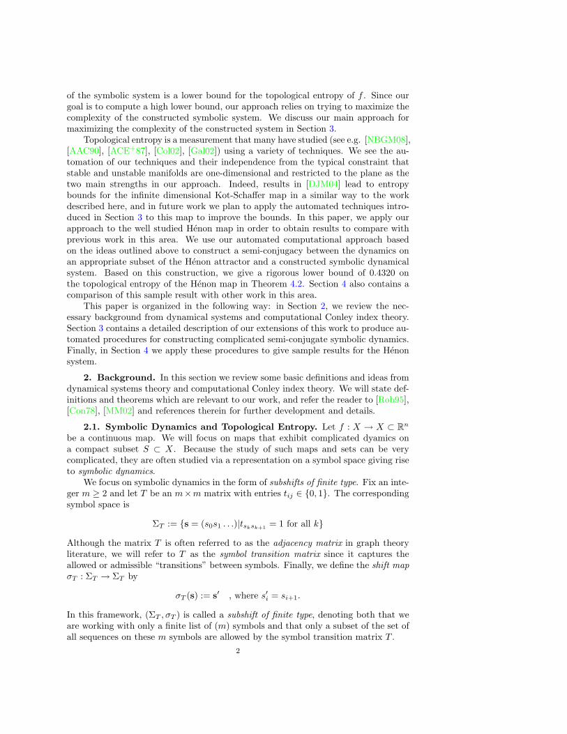
Definition 2.9. Let P = (P1, P0) be a pair of compact sets with P0 " P1 " X.The map induced on the pointed quotient space (P1/P0, [P0]) is

fP (x) :=!

f(x) if x, f(x) % P1 \ P0

[P0] otherwise (2.6)

Definition 2.10. ([RS88]) The pair of compact sets P = (P1, P0) with P0 "P1 " X is an index pair for f provided that

1. the induced map, fP , is continuous,2. P1 \ P0, the closure of P1 \ P0, is an isolating neighborhood.

In this case, we say that P is an index pair for the isolated invariant set S =Inv(P1 \ P0, f).

The following definition is required for the definition of the Conley index.Definition 2.11. Two group homomorphisms, % : G ! G and & : G! ! G!

on abelian groups G and G! are shift equivalent if there exist group homomorphismsr : G ! G! and s : G! ! G and a constant m % N (referred to as the ‘lag’) such that

r ' % = & ' r, s ' & = % ' s, r ' s = &m, and s ' r = %m.

The shift equivalence class of %, denoted [%]s, is the set of all homomorphisms & suchthat & is shift equivalent to %.

Definition 2.12. Let P = (P1, P0) be an index pair for the isolated invariantset S = Inv(P1 \ P0, f) and let fP" : H"(P1, P0) ! H"(P1, P0) be the map induced onthe relative homology groups H"(P1, P0) from the map fP . The Conley index of S isthe shift equivalence class of fP"

Con(S, f) := [fP"]s. (2.7)

The Conley index for the isolated invariant set S given in Definition 2.12 is well-defined, namely, every isolated invariant set has an index pair, and the correspondingshift equivalence class remains invariant under di!erent choices for this index pair (seee.g. [MM02]).

So far we have passed from continuous maps to induced maps on relative homol-ogy. Our overall goal, however, is to describe the dynamics of our original map. Herewe present measurements based on the map on homology that may give us informa-tion about the original map. The first theorem is Wazewski’s Principle in the contextof Conley index theory.

Theorem 2.13. If Con(S, f) &= [0]s, then S &= ,.By requiring additional structure in the isolating neighborhood N of S, we can

use a modification of Theorem 2.13 to study finer structure in S.Corollary 2.14. Let N " X be the union of disjoint, compact sets N1, . . . , Nm

and let S := Inv(N, f) be the isolated invariant set relative to N . Let

S! = Inv(N1, fNn ' · · · ' fN1) " S

where fNi denotes the restriction of the map f to the region Ni. If

Con(S!, fNn ' · · · ' fN1) &= [0]s, (2.8)6

then S! &= ,. More specifically, there exists a point in S whose trajectory under ftravels through the regions N1, . . . , Nn in the prescribed order.

We here note that given the hypotheses of Corollary 2.14, there is a nice techniquefor obtaining the index of S! given the computed index map fP", where P = (P1, P0)is an index pair with N = P1 \ P0. Using an approach developed by Szymczak in[Szy95], we set

f ijP (x) :=

!f(x) if x % Ni and f(x) % Nj

[P0] otherwise (2.9)

Then f ijP" : H"(P1, P0 * (*l (=iNl)) ! H"(P1, P0 * (*l (=jNl)). Given fPk in matrix

form representing the linear map on Hk(P1, P0), we may label the columns/rows bylocation of the associated relative homology generators in the subgroups Hk(P1, P0 *(*l (=1Nl)), . . . Hk(P1, P0 * (*l (=nNl)). To simplify notation, we say that generator g

is in region Ni if g % Hk(P1, P0 * (*l (=iNl)). Then f ijPk is the nj $ ni submatrix with

ni columns corresponding to the ni generators in Ni and nj rows corresponding tothe nj generators in Nj . Furthermore, (P1, P0 * (*l (=1Nl)) is an index pair for theisolated invariant set S! = Inv(N1, fNn ' · · · ' fN1) with index map fn1

P" ' · · · ' f12P" :

H"(P1, P0 * (*l (=1Nl)) ! H"(P1, P0 * (*l (=1Nl)). Therefore,

Con(S!, fNn ' · · · ' fN1) = [fn1P" ' · · · ' f12

P"]s (2.10)

Since the more general problem of determining whether the linear map fPk :Hk(P1, P0) ! Hk(P1, P0) is not shift equivalent to 0 may be di#cult, we here focuson a computable, su#cient condition. Trace is preserved by shift equivalence, and weadopt the notation

tr k(Con(S, f)) := tr (fPk)

where tr (fPk) denotes the trace of the linear map fPk : Hk(P1, P0) ! Hk(P1, P0).Then if tr k(Con(S, f)) &= 0 for some k, Con(S, f) &= [0]s.

Corollary 2.15. If tr k(Con(S!, fNin' · · · ' fNi1

)) &= 0 for some k then thereexists x % S! with "(x) = i1i2 . . . ini1i2 . . . in . . ..

Taking this approach we are close to showing something stronger, namely thatthere is a periodic orbit under f with the corresponding cyclic symbol sequence. Thisstronger statement relies on computing the Lefschetz number.

Definition 2.16. Let S be an isolated invariant set. The Lefschetz number ofS is defined as

L(S, f) :=#

k

(-1)k tr (fPk) (2.11)

where P = (P1, P0) is an index pair for S.The Lefschetz number is essential to the following theorem and its corollary.Theorem 2.17. Let S be an isolated invariant set. If

L(S, f) &= 0, (2.12)

then S contains a fixed point.For a proof, see [Szy96]. As before, a refinement of the approach allows us to

study symbolic dynamics.7

Corollary 2.18. Let N " X be the finite union of disjoint, compact setsN1, . . . , Nm, and let S := Inv(N, f). Let S! = Inv(N1, fNn ' · · · ' fN1) " S where fNi

denotes the map f restricted to the region Ni. If

L(S!, fNn ' · · · ' fN1) &= 0, (2.13)

then fNn ' · · · ' fN1 contains a fixed point in S! that corresponds to a periodic pointof period n in S that under f travels through the regions N1, . . . , Nn in order.

In what follows, we will develop algorithms based on Corollary 2.15 to constructand verify symbolic dynamics. However, in the special case where the index mapfP" is nontrivial on exactly one level (as occurs with the Henon map), we may useCorollary 2.18 to show that the constructed semi-conjugate symbolic systems has theadded stronger property that every periodic orbit in the symbolic system correspondsto a periodic orbit in the original system of the same period.

2.3. Multivalued and Combinatorial Maps. Now that we have the rele-vant tools from Conley index theory, we can begin applying them algorithmically toextract information about the dynamical system f : X ! X. In this section, wedescribe the construction of a combinatorial representation of f . The first step is todefine a multivalued map F that will be used to incorporate bounded errors in therepresentation.

Definition 2.19. The multivalued map F : X ! X is a map from X to itspower set, i.e. for all x % X, F (x) " X. If for a continuous, single-valued mapf : X ! X, f(x) % F (x) and F (x) is acyclic (i.e. has the homology of a point) forall x % X, then f is a continuous selector of F and F is an enclosure of f .

In what follows, we discuss how to construct an enclosure of the map under study.The purpose of the enclosure is to incorporate round-o! and other errors that occurin computations. This construction requires rigorous, small error bounds in order tocreate an enclosure whose images are not so large as to obscure all relevant dynamics.Given an appropriate enclosure, the topological tools from Section 2.2 may be used touncover dynamics of the underlying map. Furthermore, there are algorithms for boththe construction of the enclosure and the computation of the Conley index. Thesealgorithms require a further step – discretizing the domain in order to store it in thecomputer as a finite list of objects.

We begin by using the subdivision procedure implemented in the software packageGAIO [DFJ01] to create a grid G on a compact (rectangular) region in X. In prac-tice, the region chosen for representation is usually determined either experimentallythrough non-rigorous numerical simulations or analytically given a special structure orsymmetry for the system (e.g. a compact attracting region). We partition a specifiedrectangular set W =

$nk=1[x

#k , x+

k ] " Rn into a cubical grid

G(d) :=

%n&

k=1

'x#k +

ikrk

2d, x#k +

(ik + 1)rk

2d

( ))))) ik %*0, . . . , 2d - 1

+,

where rk = x+k -x#k is the radius of W in the kth coordinate and the depth d is a non-

negative integer. We call an element of the grid, B =$n

k=1

-x#k + ikrk

2d , x#k + (ik+1)rk

2d

.,

a box. For a collection of boxes, G " G = G(d), define the topological realization of Gas |G| := *B'GB " Rn.

Constructing a useful combinatorial enclosure involves bounding all round-o! andother errors. In our study of the Henon map in Section 4, we construct a combinatorial

8

enclosure by computing images of f(|G|) using interval arithmetic software. Thisproduces a bounding box, f(|G|), for the image f(|G|), which is then intersected withthe grid G to produce the combinatorial enclosure image

F(G) := {G! % G : |G!| + f(|G|) &= ,}.

This combinatorial enclosure, F : G ! G, yields an enclosure F = |F| of f in thefollowing way: define |F| : W ! W , where W = *G'G |G|,

|F|(x) :=/

G'G with x'|G|

|F(G)|. (2.14)

More importantly, e#cient algorithms exist for computing isolating neighborhoods,index pairs, and Conley indices for f from an appropriate combinatorial enclosure Fof f .

2.4. Computational Conley Index Theory. Now we give algorithms for com-puting the isolating neighborhoods, index pairs, and Conley indices first introducedin Section 2.2 in the setting of combinatorial enclosures.

Definition 2.20. A combinatorial trajectory of a combinatorial enclosure Fthrough G % G is a bi-infinite sequence $G = (. . . , G#1, G0, G1, . . .) with G0 = G,Gn % G, and Gn+1 % F(Gn) for all n % Z.

Definition 2.21. The combinatorial invariant set in N " G for a combinatorialenclosure F is

Inv(N ,F) := {G % G : there exists a trajectory $G " N}.

Definition 2.22. The combinatorial neighborhood of B " G is

o(B) := {G % G : |G| + |B| &= ,}.

This set, |o(B)|, sometimes referred to as a one box neighborhood of B in G, is thesmallest representable neighborhood of |B| in the grid G.

While there are di!erent characterizations of isolation in the setting of combina-torial enclosures, we chose the following for this work.

Definition 2.23. If

o(Inv(N ,F)) " N

then N " G is a combinatorial isolating neighborhood under F .Note that by construction, the topological realization |N | of a combinatorial iso-

lating neighborhood N under F is an isolating neighborhood under any continuousselector f % |F|. This definition is stronger than what is actually required to guaran-tee isolation on the topological level. It is, however, the definition that we will use inthis work and is computable using the following approach.

Let S " G. Set N = S and let o(N ) be the combinatorial neighborhood of N inG. If Inv(o(N ),F) = N , then N is isolated under F . If not, set N := Inv(o(N ),F)and repeat the above procedure. In this way, we grow the set N until either theisolation condition is met, or the set grows to intersect the boundary of G in whichcase the algorithm fails to locate an isolating neighborhood in G. This procedure isoutlined in more detail in the following algorithm from [DJM04].

Algorithm 1 (Grow Isolating Neighborhood).

9

INPUT: grid G, combinatorial enclosure F on G, set S " GOUTPUT: a combinatorial isolating neighborhood N containing S

or N = , if the isolation condition is not met

N = grow isolating neighborhood(G, F, S)G boundary:= {G % G : |G| + '|G| &= ,};N := S;while Inv(o(N ),F)) &" N and N + G boundary= ,,

N := Inv(o(N ),F);endif N + G boundary= ,, return N;else return ,;end

Once we have an isolating neighborhood for f , our next goal is to compute acorresponding index pair. The following definition of a combinatorial index pair againemphasizes our goal of using the combinatorial enclosure to compute structures for f .

Definition 2.24. A pair P = (P1,P0) of cubical sets is a combinatorial indexpair for a combinatorial enclosure F if the corresponding topological realization P =(P1, P0), where Pi := |Pi|, is an index pair for any continuous selector f % |F|.Namely, P1 \ P0 = |P1 \ P0| is an isolating neighborhood under f and the map fP , asdefined in Definition 2.9, is continuous.

The following algorithm produces a combinatorial index pair associated to a com-binatorial isolating neighborhood produced via Algorithm 1. While there are otheralgorithms for producing combinatorial index pairs, this algorithm works well withlater index computations. For more details, see the description of modified combina-torial index pairs in [Day03].

Algorithm 2 (Build Index Pair).INPUT: grid G, combinatorial enclosure F on G,

combinatorial isolating neighborhood N produced by Algorithm 1OUTPUT: combinatorial index pair P = (P1,P0) with P1 \ P0 = N

[P1,P0] = build index pair(G, F, N)P0 := ,;New := F(N ) + o(N ) \ N;while New &= ,

P0 := P0 *New;New := (F(P0) + o(N )) \ P0;

endP1 := N * P0;return [P1, P0];

We now have an isolating neighborhood |N | and corresponding index pair P :=(|P1|, |P0|) for f . What remains in computing the Conley index for the associatedisolated invariant set, S := Inv(|N |, f), is to compute the map fP" : H"(|P1|, |P0|) !H"(|P1|, |P0|). Once again, the combinatorial enclosure o!ers the appropriate compu-tational framework and we use the software program homcubes in [Pil98] to computefP". This step is outlined in Algorithm 3.

10

Algorithm 3 (Compute Index Map).INPUT: grid G, combinatorial enclosure F on G,

combinatorial index pair P = (P1,P0) produced by Algorithm 2OUTPUT: relative homology groups H"(|P1|, |P0|),

the induced index map fP" : H"(|P1|, |P0|) ! H"(|P1|, |P0|),and the induced submaps {f ij

Pk} on connected components

[fP" H"(|P1|, |P0|) {f ijPk}] = compute index map(G, F, P1, P0)

Q1 = F(P1);Q0 = F(P0);[fP" H"(|P1|, |P0|) {f ij

Pk}] := homcubes(P1, P0, Q1, Q0, F);return [fP" H"(|P1|, |P0|) {f ij

Pk}];

Algorithm 3 produces a sequence of matrices for the maps fP0, fP1, . . . , fPn

where n is the dimension of the phase space X. For k > n, fPk = 0. The asso-ciated Conley index is Con"(S) = [fP"]s, for S := Inv(|P1 \ P0|, f). The submapsf ij

Pk : Hk(|P1|, |P0| *l (=i |Nl|) ! Hk(|P1|, |P0| *l (=j |Nl|), where |N1|, . . . |Nn| are theconnected components of |P1 \ P0|, are given as submatrices of fPk. These are themaps required for Corollaries 2.14, 2.15, and 2.18. In the following section, we describean algorithmic procedure for using this index information to construct the appropriatesubshift of finite type.

3. Constructing and Verifying Complicated Symbolic Dynamics. Givenf : X ! X, the general method we adopt for computing a lower bound on topologicalentropy consists of the following steps:

• constructing a fixed cubical grid G on a subset of X and a combinatorialenclosure F of f on G (Section 2.3),

• locating a region of interest S in G (Section 3.1),

• computing the associated Conley index (Section 2.4),

• constructing semi-conjugate symbolic dynamics (Section 3.2),

• using the constructed symbolic dynamical system to compute a lower boundon the topological entropy of f (Theorem 2.7).

While many steps of this general procedure have been carried out in previous work(e.g. [DJM04] for the first four steps, and [Gal01] for the last step), we here seek touncover far more complicated symbolic dynamics. This requires a more automatedapproach based on setting verifiable conditions for uncovering and proving the ex-istence of cyclic symbolic dynamics and ignoring or giving up on the verification ofdynamics that does not satisfy these conditions. Along these lines, we now give al-gorithms for locating a region of interest (Section 3.1) and processing the resultingindex information (Section 3.2) that allow us to uncover more complicated dynamicsthan previously found using related techniques. This improved procedure producesthe entropy bounds presented in Section 4.

11

3.1. Locating a region of interest. We now turn to the second task in this list– that of locating the region of the grid where we will attempt to compute interestingsymbolic dynamics. More specifically, the set that we are calling the region of interestwill serve as the input, S, for Algorithm 1. We show three di!erent methods forlocating regions of interest for the Henon map in Sections 4.1, 4.2, and 4.3. In thissection, we focus on the method that, of these three, is both general (i.e. is notrestricted to studies of the Henon map) and yields high entropy bounds. This isthe method followed in Section 4.2. The first step in this approach is similar inspirit to the work of Cvitanovic and others in using periodic orbits of low periods toapproximate chaotic attractors. We begin by finding short cycles in the combinatorialenclosure (directed graph) F . These short cycles correspond to possible periodic orbitsof low period for f . We then add a level of complexity by searching for paths in thedirected graph between these short cycles. From a dynamics point of view, thesepaths represent possible mixing between the periodic regions.

We construct a list of short cycles in G by setting a computational parameterMax Cycle Length % Z+, and locating the cycles in F of length k with 1 ( k (Max Cycle Length. These cycles are nonzero entries on the diagonal of F (whenviewed as a transition matrix) raised to the kth power. The corresponding computedvertices in F are the regions in G that may contain period k points of f . Starting withS = ,, we begin adding the short cycles to S one by one, starting with the shortest.Just before adding a cycle to S, we grow its isolating neighborhood using Algorithm 1and then check that this neighborhood does not intersect the isolating neighborhoodof the current collection. This corresponds to a possible increase in the number ofsymbols and/or the number of admissible transitions between symbols in the resultingconstructed symbolic system and may eventually lead to a higher entropy bound. Ifthis condition is not met, we do not add the cycle and move to the next cycle in thelist, continuing until the list is exhausted. We next use breadth first search (BFS) tofind shortest path, pairwise connections between the short cycles in S and add theseconnecting paths to S. This procedure is outlined in Algorithm 4.

Algorithm 4 (Locating Region of Interest/Joining Low Cycles).INPUT: grid G, combinatorial enclosure F on G,

computational parameter Max Cycle LengthOUTPUT: region of interest S " G

S = find and connect low cycles(G, F, Max Cycle Length)S = ,;N = ,;for n = 1 : Max Cycle Length,

for each length n cycle c in F,Nc = grow isolating neighborhood(G, F, c);if Nc +N = ,,

S = S * c;N = grow isolating neighborhood(G, F, N * c);

endend

endSc := S;for each vertex vi % Sc,

12

A !! B !!

""

C !! D !! E !!

""

F !! G

##

N

$$

M%% L%% K

$$

%% J%%

&&!!!!!!!I%% H

''

%%

Fig. 3.1. Symbol transition graph constructed from a 2-cycle, two 4-cycles, and pairwise con-nections.

for each vertex vj % Sc,$ = shortest path in F from vi to vj in G\o(o(S));S := S * $;

endendreturn S;

Here, we explicitly compute cycles with lengths up to Max Cycle Length, whichin practice is small. However, we obtain many new cycles by adding pairwise connec-tions between the computed cycles. This allows us to uncover complicated dynamicswithout having to explicitly search for the long cycles that correspond to periodicorbits of high period. As illustration, Figure 3.1 depicts a subshift of finite type con-structed from a region of interest consisting of a length 2 cycle, two length 4 cyclesand pairwise shortest connecting paths between these three objects. Note that the re-sulting subshift system contains infinitely many cycles (of lengths 5, 8, 10 and higher)and positive topological entropy.

While e!ective in computation of entropy bounds for the Henon map (see Sec-tion 4.2), this approach for the construction of the region of interest, S, could beimproved. Given a fixed combinatorial enclosure F on a grid G, one goal would be tooptimize the construction of S in order to produce a subshift of finite type with thehighest possible entropy. As a first step along these lines, the relationship betweenthe entropy bound and the maximal cycle length used in Algorithm 4 in a study ofthe Henon map is depicted in Figure 4.4. In addition, there is a clear trade-o! be-tween refining the grid in order to find, isolate, and connect more low period cyclesto produce a higher bound and the associated increase in computational cost. (Thee!ect of refining the grid on increasing the bound is illustrated for the Henon map inFigure 4.5.) Another improvement to these techniques related to this balance wouldinvolve making the computation of G, and therefore S, adaptive. The goal here wouldbe to refine the grid in areas where new low period periodic orbits and connectionsmay be uncovered without having to recompute structures in the remainder of thespace.

3.2. Processing Index Information. Recall that our goal is to compute com-plicated symbolic dynamics. If we are successful in locating an appropriate region ofinterest in the domain (one approach is described in Section 3.1), the correspondingConley index computed by the algorithms described in Section 2.4 is given as a largematrix representing the map induced on an index pair consisting of many disjointcomponents.

From this index map, we wish to find a symbol transition matrix T such that f issemi-conjugate to the subshift on "T . We first use some properties of shift equivalenceto simplify the computed index map. We then construct T from a collection of cycles,called verified cycles, that satisfy the hypotheses of Corollary 2.15.

13

3.2.1. Removing Transient Generators. We begin our processing of the in-dex map fP" : H"(P1, P0) ! H"(P1, P0) by removing generators from H"(P1, P0) thatdo not correspond to asymptotic invariant behavior. More specifically, we utilize thefact that the Conley index, Con"(S, f), is the shift equivalence class of fP" to constructa new representative of the class obtained by removing generators ( % Hk(P1, P0) suchthat f l

Pk(() = 0 or ( /% f lPk(Hk(|P1|, |P0|)) for some l % Z.

Note that since we are considering continuous maps f on Rn, fPk : Hk(P1, P0) !Hk(P1, P0) are linear maps on (finite) vector spaces. We therefore choose to think offPk as a square matrix. Suppose that fPk is similar to a matrix A, i.e. fPk = B#1ABfor some invertible matrix B. Then, by setting r = B, s = B#1, and m = 0 inDefinition 2.11, we see that [fPk]s = [A]s. In what follows, B will be an appropriatereordering of the basis so that A takes on the block lower triangular form required forthe following theorem.

Theorem 3.1. Let

A =

0

1A11 0 0A21 A22 0A31 A32 A33

2

3

be a 3$ 3 block lower-triangular matrix, with square matrices Aii on the diagonal. IfAl

11 = 0 and Al33 = 0 for some l, then A is shift equivalent to A22.

Proof. For i = 1, 2, 3, let ni $ ni be the size of the square matrix Aii, and defineprojection and inclusion maps respectively as follows:

) =40n22)n11 In22 0n22)n33

5

and

* = )*.

One can check that the maps R := )Al and S := Al* satisfy the conditions statedin Definition 2.11 to give the desired shift equivalence between A and A22 with lagconstant m = 2l.

The motivation for the previous theorem was to find a simpler representative forthe shift equivalence class of fPk. This relies on finding a reordering of the basisfor fPk that yields a similar matrix A satisfying the hypotheses of Theorem 3.1. Inorder to use existing e#cient algorithms, we now turn to a graph interpretation of thel $ l matrix fPk. More specifically, we consider the directed graph G = (V,E) withvertices 1, . . . , l and edges (j, i) % E if and only if fPk(i, j) &= 0. Let

V3 := {v % V | any path starting at v has length less than l} (3.1)

V1 := {v % V \ V3| any path ending at v has length less than l}. (3.2)

and

V2 := V \ (V1 * V3). (3.3)

Note that since there are l vertices, V1 is the set of vertices that are not connectedto cycles in backward time and V3 is the set of all vertices that are not connected tocycles in forward time. The following two lemmas show that the partition {V1, V2, V3}of the vertex set V is useful for finding zeros in the matrix fPk.

14

Lemma 3.2. The submatrix fPk(V1, V2 * V3) of fPk corresponding to the rowsindexed by V1 and columns indexed by V2 * V3 is the zero matrix of the appropriatesize.

Proof. Suppose that fPk(w, v) &= 0 for w % V1 and v % V2 * V3. Then (v, w) isan edge in the associated directed graph G. Since v is not in V1, there exists a pathv1, . . . , vl, v in G. Then v1, . . . , vl, v, w is a length l + 1 path in G, contradicting ourassumption that w % V1.

Lemma 3.3. The submatrix fPk(V2, V3) of fPk corresponding to the rows indexedby V2 and columns indexed by V3 is the zero matrix of the appropriate size.

Proof. Suppose that fPk(w, v) &= 0 for w % V2 and v % V3. Then (v, w) is anedge in the associated directed graph G. Since w is not in V3, there exists a pathw, v1, . . . , vl in G. Then v, w, v1, . . . , vl must also be a path in G, contradicting ourassumption that v % V3.

We have now shown that if we reorder the basis by listing the basis elements inV1, followed by those in V2, followed by those in V3, we obtain the following blockform (with rows and columns labeled by location in the specified sets):

fPk . A =

6

7

V1 V2 V3

V1 A11 0 0V2 A21 A22 0V3 A31 A32 A33

8

9

What remains to show in order to use Theorem 3.1 is the following lemma.Lemma 3.4. The two matrices, Al

11 and Al33, are zero matrices of the appropriate

sizes.Proof. We obtained the block lower triangular matrix A by a reordering of the

basis for the matrix fPk. Therefore, the associated directed graph GA for A is thedirected graph G with relabeled vertices. With a slight abuse of notation, we consideragain the subsets V1, V2, V3 in GA to be the sets satisfying (3.2), (3.3), and (3.1)respectively. Interpreting nonzero entries of A to be weights on the correspondingedges, we may use powers of A to study paths in GA. More specifically, Al(i, j) &= 0implies that there exists a length l path from vertex j to vertex i in GA (see, e.g.[Die05]). Now suppose that Al(i, j) = Al

11(i, j) &= 0 for some i, j % V1. Then by theabove argument, there exists a length l path in GA that ends at a vertex in V1. Thiscontradicts (3.2). Therefore, Al

11 = 0. A similar argument shows that Al33(i, j) = 0

for all i, j % V3.We now have that fPk is similar (and hence shift equivalent) to A which is shift

equivalent to fPk := A22 by Lemma 3.4 and Theorem 3.1. Therefore, we may takefPk to be the new, possibly smaller representative of the Conley index

Con(S, f) = [fPk]s = [fPk]s.

This procedure is outlined in Algorithm 5. Here, algorithms based on depth or breadthfirst search may be used to e#ciently compute the required sets V1, V2, and V3. Aswe will show in Section 4 this technique may give a drastic decrease in the size of therepresentative index map.

Algorithm 5 (Remove Transient Generators).INPUT: square matrix fPk

OUTPUT: shift equivalent (square) matrix fPk

15

fPk = remove transient generators(fPk)G = (V,E) is the directed graph associated to fPk;V3 = {v % V | any path starting at v is finite};V1 = {v % V | any path ending at v is finite};V2 = V \ (V1 * V3);fPk = fPk(V2, V2);return fPk;

3.2.2. Cycle verification. We now automate a procedure for using Conley in-dex computations to construct a semi-conjugate subshift of finite type. As describedin Theorem 3.6 below, we construct the subshift system from a collection of cyclesthat are verified using Corollary 2.15. As will be seen in Section 4, the automationof this procedure becomes necessary as we build increasingly complicated subshiftsof finite type. In particular, building a subshift system containing infinitely manyperiodic orbits may, in principle, lead to an infinite list of computations to verifythat the hypotheses of Corollary 2.15 hold for each cycle. In the following approach,we present an algorithm which uses a finite list of computations to verify a possiblyinfinite set of cycles.

Given an index pair P = (P1, P0), we begin by labeling each of the (m) disjointregions of the isolating neighborhood N := P1 \ P0. Let N = *m

i=1Ni with Ni closedand nonempty and Ni + Nj = , for all i &= j. By construction, each Ni has acorresponding cubical representation Ni " N . Recall that the associated itineraryfunction " is defined by "(x) = (s0s1 . . .) with sj = i if f j(x) % Ni. Let T be the matrixof admissible transitions between the regions Ni allowed by F . More specifically, Tis the m$m matrix with entries

tij =!

1 if F(Nj) +Ni &= ,0 otherwise. (3.4)

Then " : S ! "T where S := Inv(N, f) and "T and !T : "T ! "T are the subshiftof finite type defined in Section 2. As previously discussed, " : S ! "T may not besurjective and, hence, !T : "T ! "T may not be semi-conjugate to f : S ! S. Wewill now construct a subshift system, !T : "T ! "T , with "T " "T , that we proveis semi-conjugate via " to f : S ! S with S " S.

Let G = (V,E) be the directed graph associated to the symbol transition graphT (viewed as an adjacency matrix). More specifically, the vertices are named for theregions, Ni with V = {1, 2, . . . m} and the edge set E := {(j, i) % V $ V |tij = 1}represents the admissible transitions between regions. In our approach, we begin byremoving all paths in G that are not contained in cycles. These paths correspondto dynamics that we will not check using index theory. A practical way to performthis step is to remove edges and vertices not contained in the strongly connectedcomponents (SCC) of G. We will now study Conley indices for periodic symbolsequences in "T represented by cycles in G.

As discussed in Section 2.2, we consider restricted index maps

f ijPk : Hk (P1, P0 * (*l (=iNl)) ! Hk(P1, P0 * (*l (=jNl)).

To do this, we first group the generators of Hk(P1, P0) remaining after running Al-gorithm 5 by region Ni. Again, thinking of fPk as a matrix with rows and columns

16

corresponding to the generators of Hk(P1, P0), we have that

f ijPk := fPk(gNj , gNi) (3.5)

where gNi are the (row/column) indices of generators in Hk(P1, P0 *:

l (=i Nl) "Hk(P1, P0). Here, f ij

Pk is as an nj $ ni matrix where ni and nj are the numberof generators in regions Ni and Nj respectively. To simplify notation, for a pathp = (s1, s2, . . . , sn), let

fpPk := fsn!1sn

Pk ' · · · ' fs1s2Pk . (3.6)

Definition 3.5. We say that a cycle, c = (s1, s2, . . . , sn, s1) in G is verified iffor some k,

tr (fcPk) = tr k Con(S!, fNsn

' · · · ' fNs1) &= 0

where S! := Inv(Ns1 , f |Nsn$Ns1' · · · ' f |Ns1$Ns2

). Note that by Corollary 2.15,"#1(s) &= ,, where s = (s1s2 . . . sns1 . . . sn . . .) is the periodic symbol sequence corre-sponding to the verified cycle.

Before discussing our automated approach for verifying cycles, we give the fol-lowing theorem to serve as motivation for this work.

Theorem 3.6. Let "T be the space of symbol sequences with symbol transitionmatrix T and let Per("T ) be the set of periodic symbol sequences in "T under !T .Suppose that "T = Per("T ) and for each s = (s1 . . . sns1 . . . sn . . .) % Per("T ), thecorresponding cycle c = (s1, s2, . . . , sn, s1) in G has been verified according to Defini-tion 3.5. Then the itinerary function " is a semi-conjugacy between f : S ! S and!T : "T ! "T , where S := "#1("T ) " S.

Proof. The itinerary function, " : S ! "T is continuous and " ' f = !T ' " (seeSection 2 and references therein). Furthermore, since each cycle in G correspondingto a periodic symbol sequence in "T has been verified according to Definition 3.5, "maps onto Per("T ). Since " is continuous, S := Inv(N, f) is compact, and "T isHausdor!, " must map onto the closure of the set of of periodic symbol sequences,Per("T ) = "T . Therefore, " : S ! "T is a semi-conjugacy.

The list of cycles that may be verified according to Definition 3.5 relies im-plicitly on the form of fP and, more specifically, on f ij

Pk for k = 0, 1, 2, . . . andi, j % {1, . . . ,m}. For the examples studied in Section 4, the homology maps fPk

are trivial for all k &= 1. Therefore, for these examples we fix k = 1, as any otherchoice will necessarily lead to a zero trace and failure to verify all cycles. For di!erentsystems, there may be more flexibility in the choice of k. Given a fixed k, the questionof how the list of verified cycles relies on choices of i and j is far more subtle. Webegin this discussion by fixing k and considering the case where each region containsexactly one homology generator (ni = 1 for all i = 1, . . . ,m). We will then discussthe more di#cult case where some regions have multiple homology generators.

Note that if there is only one generator per region, then f ijPk is a scalar for all

admissible transitions tji = 1 in T . In this case, if f ijPk &= 0 for all admissible transi-

tions, then for any admissible periodic symbol sequence s = (s1s2 . . . sns1s2 . . . sn . . .)with corresponding cycle c = (s1s2 . . . sns1), tr (fc

Pk) &= 0, and, therefore, all cycles inG are verified. If, on the other hand, f ij

Pk = 0 for some admissible transition, thenany cycle c with edge (i, j) will have tr (fc

Pk) = 0 and cannot be verified using thisapproach. In this case, we remove this transition from the set of admissible transi-tions by removing the edge (i, j) from G and, correspondingly, by setting tji = 0 in

17

T . In essence, cycle verification computations in the setting where there is exactlyone homology generator per component boil down to a (finite) check that entries infPk corresponding to admissible transitions in T are nonzero.

If there are regions that contain more than one generator of homology, thenthese computations become more complicated. In what follows, we will systematicallyprocess the cycles in G. In the first phase of the procedure, we process paths andcycles in G in an attempt verify cycles. Alternatively, one can think about identifyingall cycles that may not be verified by our approach. Along these lines, we will labelcertain cycles as unverifiable and certain paths as unconcatenable. From these, wewill identify a collection of edges that need to be removed from the graph so thatall remaining cycles are verified cycles. Note that in what follows, labeling a pathunconcatenable does not mean that cycles containing this path may not be verifiedaccording to Definition 3.5, only that we may not verify some such cycles using ourprescribed list of finite computations. Let Max Iter be a nonnegative integer thatwill serve as a computational parameter.

Definition 3.7. Define the edge set for a path p = (v0, . . . , vn) to be

E(p) := {(vi, vi+1) % E(G)|i = 0, . . . , n- 1}

and the length of p to be |p| = n. Consider a cycle c = (s, v2, v3, . . . , vn#1, s) startingand ending at vertex s. If tr (fc

Pk) = 0, then c is unverifiable. (See also Definition 3.5.)A path p = (s, v2, v3, . . . , vn#1, t) from s to t of length |p| ( Max Iter, is uncon-

catenable if fpPk = 0.

For a path p = (s, v2, v3, . . . , vn#1, t) from s to t of length |p| = Max Iter, pis concatenable if there exists a path p! from s to t with |p!| < Max Iter, E(p!) /E(p), and fp

Pk = (fp"

Pk &= 0 for some ( &= 0. If no such path p! exists, then p isunconcatenable.

Finally, an edge set E is prohibited (at computational parameter Max Iter) if atleast one of the following holds:

1. there exists an unverifiable cycle c with |c| ( Max Iter and E(c) / E

2. there exists an unconcatenable path p with E(p) / E

Lemma 3.8. If c is a cycle whose edge set E(c) is not prohibited then c is averified cycle.

Proof. Suppose that |c| ( Max Iter. Since E(c) is not prohibited, c must be averified cycle.

Next, notice that in the natural partial ordering on edge sets, if E! is prohibitedthen so is E for any E containing E!. Therefore, E(c) must not contain any prohibitedsubsets. If |c| > Max Iter, then c is the concatenation of 2 paths, p1 and p2, where|p2| = Max Iter. We will use the notation p1p2 to denote the concatenation of pathsp1 and p2. Label the start/end vertices s1, t1 and s2, t2 of p1 and p2 respectively. Notethat s1 = t2 and t1 = s2 by construction. Since E(p2) / E(c) is not prohibited, thereexists a path p!2 from s2 to t2 with E(p!2) / E(p2), |p!2| < Max Iter, and fp2

Pk = (fp"2Pk

for some ( &= 0. Therefore,

fcPk = fp2

Pkfp1Pk

= (fp"2Pkfp1

Pk

= (fc"

Pk

18

where c! = p1p!2 is a cycle with E(c!) = E(p1)*E(p!2) / E(c) and length |c!| ( |c|-1.Continuing this process, we obtain a cycle c with |c| ( Max Iter, E(c) / E(c), andfc

Pk = (f cPk for some ( &= 0. Since E(c) cannot be prohibited, c must be verifiable

and

tr (fcPk) = tr ((f c

Pk) = (tr (f cPk) &= 0.

Therefore, c is a verified cycle.Lemma 3.8 and Theorem 3.6 provide an outline of our approach for constructing

the semi-conjugate system. By Lemma 3.8, we know that all cycles that do nothave prohibited edge sets are verified cycles and may be used to construct the semi-conjugate system according to Theorem 3.6. In practice, we use the prohibited edgesets to identify a collection of edges to be removed from G, resulting in the desiredsemi-conjugate system.

We now give an outline of our procedure for locating prohibited edge sets bycollecting and testing appropriate matrix products along paths in G. The algorithmoutputs a collection of minimal prohibited edge sets B, that is for any prohibited edgeset E, there is a prohibited edge set E! % B with E! / E.

Algorithm 6 (Find Prohibited Edge Sets).INPUT: graph G, index map fPk, computational parameter Max Iter;OUTPUT: list of minimal prohibited edge sets B

B = find prohibited edge sets(G, {fPk}, Max Iter)B = ,;for all s, t % V (G), E " E(G), set all M(s, t, E, k) = ,;for all (s, t) % E(G),if s == t and tr (fst

Pk) == 0, B = B * {(s, t)};else M(s, t, {(s, t)}, 1) = {fst

Pk};end

end

for k = 1.. Max Iter,for s, t % V (G), E / E(G), M %M(s, t, E, k),for (t, u) % E(G),

E! = E * (t, u);M ! = f tu

PkM;if (M ! == 0) or (s == u and tr (M !) == 0),B = B * {E!};set M(s!, t!, E!!, +) = , for all s!, t! % V (G), E! / E!! / E(G), + ( k;

else if & 0M !! %:

!<kE""+E"

M(s, t, E!!, +), with M !! == (M ! for some ( &= 0,

M(s, t, E!, k + 1) = M(s, t, E!, k + 1) * {M !};end

endend

end

B = B * {E " E(G) | M(s, t, E, Max Iter) &= , and E minimal};return B;

19

In practice, it is more e#cient to apply Algorithm 6 only to a subgraph of G thatcaptures the behavior of the system in the regions with multiple homology generators.More specifically, we first study G restricted to the vertices for multiple generatorregions and the neighboring single generator regions. This allows us to take advantageof the fact that fp

Pk is a scalar for all paths p starting and ending at vertices forsingle generator regions. By removing enough edges so that there are no remainingprohibited edge sets in the subgraph, we can reduce the check that cycles remainingin G are verified to a check that the maps f ij

Pk between single generator regions arenonzero. This is the approach we adopt for the results described in Section 4.

For all cycles c in G that do not contain any prohibited edge sets (listed in B), cis a verified cycle by Lemma 3.8. What remains for the construction of a subgraphG! of verified cycles, is to remove enough edges so that we no longer have any cycleswith prohibited edge sets. Since our goal is to obtain a high lower bound for entropy,we will select one edge from each prohibited edge set so that the removal of theseedges results in the semi-conjugate symbolic system with highest entropy. Again,since the list of prohibited edge sets is finite (and each prohibited edge set is finite),the computation of optimal edges to remove is finite. Removing the edges yields agraph in which all cycles may be verified using Corollary 2.15. By Theorem 3.6, thecorresponding adjacency matrix, T , defines a semi-conjugate symbolic system.

The following is an outline of the procedure for breaking prohibited edge sets.

Algorithm 7 (Break Prohibited Edge Sets).INPUT: graph G, a list of prohibited edge sets B,OUTPUT: graph G! in which all cycles may be verified via Corollary 2.15

G! = break prohibited edge sets(G, B)if B = ,, return G! = G;hmax = -1;Ec = ,;for each set {e1, e2, . . . , eN}, where ei is an edge on the ith cycle in B,let G! be the subgraph of G obtained by removing edges e1, e2, . . . , eN;let T (G!) be the adjacency matrix for G!;h = log(sp(T (G!)));if h > hmax,

hmax = h;Ec = {e1, e2, . . . , eN};

endendlet G! be the subgraph of G obtained by removing the edges in Ec;return G!;

Combining Algorithms 6 and 7, Theorem 3.6 guarantees that the following algo-rithm produces a symbol transition matrix T with ! : "T ! "T semi-conjugate tof : S ! S. Noting that f ij

Pk = 0 will cause the verification procedure to fail for anycycle containing edge (i, j), we will start with a graph G on the same vertex set withthe edge set E = {(i, j)|f ij

Pk &= 0}.

Algorithm 8 (Build Subshift).INPUT: index map fPk : Hk(|P1|, |P0|) ! Hk(|P1|, |P0|),

20

computational parameter Max IterOUTPUT: symbol transition matrix T for semi-conjugate subshift of

finite type

T = build subshift(fPk, Hk(|P1|, |P0|), Max Iter)fPk = remove transient generators(fPk);set m to be the number of disjoint components of Hk(|P1|, |P0|);V = {1, . . . ,m};E = {(i, j) % V $ V |f ij

Pk &= 0};G = G(V,E);G = SCC(G); (removes all edges not contained in cycles)U = find prohibited edge sets(G, fPk, Max Iter);G! = break prohibited edge sets (G, U);T is the adjacency matrix for graph G!;return T;

4. An example: the Henon map. As illustration, we now apply our tech-niques to the Henon map

h(x, y) = (1 + y - ax2, bx) (4.1)

at the classical parameters a=1.4, b=0.3. Since its first appearance in [Hen76], therehas been extensive research on the Henon map. The first result concerning a realdescription of the chaotic dynamics of the Henon map is [MS80], where the existenceof a transverse homoclinic point, and hence the existence of horseshoe dynamics, isproved. In [Szy97], Szymczak used Conley index theory to give a computer-assistedproof of the existence of periodic orbits of all periods except three and five. In [Gal02],Galias employed the method of covering relations (related to Easton’s windows) togive a computer-assisted proof of the existence of an infinite number of homoclinicand heteroclinic trajectories. [Gal02] also contains a result which gives a rigorouslower bound for the topological entropy of the map htop(h) # 0.4300. In [NBGM08],Newhouse et al. use the planar structure of the Henon map to compute htop(h) #0.46469, the highest lower bound on the entropy for Henon at the classical parametervalues currently reported.

For this work, we use the GAIO software package to construct grids, G(d), atdiscretization depths 0 ( d ( 12, on the initial box [-1.425, 1.425] $ [-0.425, 0.425](see Section 2.3). We then use the interval arithmetic package INTLAB [Cse99] tocompute a combinatorial enclosure, H, on G(d) as

H(I1 $ I2) = {G % G(d)|h(I1, I2) +G &= ,}

where I1 $ I2 is an element in G(d) in interval product notation and h(I1, I2) denotesthe rectangular image of h(I1, I2) computed using (outward rounding) interval arith-metic. Finally, we use Matlab scripts encoding the algorithms outlined throughoutthe paper to find and compute the required Conley index structures and subshifts offinite type. In the following sample results, we describe three di!erent techniques forproducing the region of interest S " Gd. Given S, the main approach is the following:

Algorithm 9 (Main).INPUT: grid Gd, combinatorial enclosure H on G,

21

(a)

C !! E

""

A

$$

F

""

%%

D

$$

((B))

(b)

Fig. 4.1. (a) A combinatorial index pair, (P1,P0), computed using Algorithms 1 and 2 for theHenon map at depth d = 7. (P0 is the collection of boxes shown in cyan.) (b) The correspondingsymbol transition graph produced by Algorithm 8.

region of interest S, computational parameter Max IterOUTPUT: lower bound on the topological entropy of h ENTROPY

ENTROPY = compute entropy lower bound(Gd, H, S, Max Iter)ENTROPY = 0;N = grow isolating neighborhood(S); (Algorithm 1)[P1,P0] = build index pair(N); (Algorithm 2)fP" = compute index map(P1, P0, H, Gd); (Algorithm 3)for k = 1..dim(Gd), with fPk &= 0,

T = build subshift(fPk, Hk(|P1|, |P0|), Max Iter); (Algorithm 8)ENTROPY := max{ENTROPY, log(sp(T ))};

endreturn ENTROPY;

4.1. Joining two short cycles. For purposes of illustration, we begin with arelatively simple example on the grid at depth d = 7. Although the resulting entropylower bound, 0.2406, is small, this example provides us with matrices of reasonablesizes for depicting the results of various stages of the procedure. For this example,we locate a region of interest, S, by searching the computed enclosure H on G(7) fora cycle of length 2, a cycle of length 4 and shortest path connections from the 2-cycleto the 4-cycle and from the 4-cycle to the 2-cycle. S is the union of these four objects.Applying Algorithms 1 and 2 to S result in the index pair given in Figure 4.1.

Theorem 4.1. The topological entopy of the Henon map (4.1) is bounded frombelow by 0.2406.

22

Proof. The computed index map for the index pair depicted in Figure 4.1(a) is

hP,1 =

6

;;;;;;;;;;;;;;7

A B B B B C D E F F

A 0 0 0 0 0 0 -1 0 0 -1B 0 0 0 0 0 0 -1 0 0 0B 0 0 0 0 0 0 0 0 0 0B 0 0 0 0 0 0 0 0 1 0B 0 0 0 0 0 0 0 0 1 0C 1 0 0 0 0 0 0 0 0 0D 0 1 0 1 0 0 0 0 0 0E 0 0 0 0 0 1 0 0 0 0F 0 0 0 0 0 0 0 -1 0 0F 0 0 0 0 0 0 0 1 0 0

8

<<<<<<<<<<<<<<9

The rows and columns are labeled by location of the corresponding homology genera-tor in the labeled regions of the isolating neighborhood (see Figure 4.1(a)). ApplyingAlgorithm 5 for removing transient generators to hP,1 produces the shift equivalentmatrix

A =

6

;;;;;;;;;;7

A B B C D E F F

A 0 0 0 0 -1 0 0 -1B 0 0 0 0 -1 0 0 0B 0 0 0 0 0 0 1 0C 1 0 0 0 0 0 0 0D 0 1 1 0 0 0 0 0E 0 0 0 1 0 0 0 0F 0 0 0 0 0 -1 0 0F 0 0 0 0 0 1 0 0

8

<<<<<<<<<<9

This is the matrix labeled A22 in Theorem 3.1 and is obtained by an appropriatereordering of the basis. Note that this algorithm removed two of the homology gen-erators in region B and, therefore, reduced the size of the representative of the shiftequivalence class/Conley index.

As an example computation, using Corollary 2.15 to verify the cycle (B, D,B),we check that

tr 1(Con(S!, f |D$B ' f |B$D)) = tr=hDB

P,1 hBDP,1

>

= tr 1

?'-1

0

( 41 1

5@

= tr 1

?'-1 -1

0 0

(@

&= 0.

Running Algorithm 8 on A to verify a collection of cycles results in the construc-tion of a semi-conjugate subshift system with symbol transition matrix

T =

6

;;;;;;7

A B C D E F

A 0 0 0 1 0 1B 0 0 0 1 0 1C 1 0 0 0 0 0D 0 1 0 0 0 0E 0 0 1 0 0 0F 0 0 0 0 1 0

8

<<<<<<9.

23

Fig. 4.2. The combinatorial index pair, (P1,P0), constructed starting with Algorithm 4 forTheorem 4.2 at depth 12. (P0 is the collection of boxes shown in cyan.)

The corresponding symbol transition graph is given in Figure 4.1(b). Since the log ofthe spectral radius of T is greater than 0.2406, the result follows from Theorem 2.7.

4.2. Joining low cycles (Algorithm 4). We now focus on improving thebound by refining the grid and using Algorithm 4 to compute a more complicatedregion of interest.

This approach results in the following theorem.Theorem 4.2. The topological entopy of the Henon map (4.1) is bounded from

below by 0.4320.Outline of Proof. Given the enclosure H on G(12), we use Algorithm 4 with

Max Cycle Length=7 to produce the region of interest S. We then follow Algo-rithm 9. The index pair for S appears in Figure 4.2. Algorithm 3 returns an indexmap on 1521 relative homology generators. Algorithm 5 reduces this map to a shiftequivlalent map on 309 generators. Finally, Algorithm 8 produces a semi-conjugatesubshift of finite type with 247 symbols. The symbol transition matrix for the con-structed subshift is depicted in Figure 4.3. The log of the spectral radius of T isbounded from below by 0.4320. The result then follows from Theorem 2.7. "

For the above result computed on the grid G(12), we choose the maximal cyclelength for Algorithm 4 to be Max Cycle Length= 7. This choice is made becausechoosing Max Cycle Length< 7 yields a lower bound than that given in Theorem 4.2,and choosing Max Cycle Length> 7 yields an entropy lower bound of 0. This behavioris depicted in Figure 4.4. The reason that choosing a large maximal cycle length leads

24

0 50 100 150 200

0

20

40

60

80

100

120

140

160

180

200

Fig. 4.3. A depiction of the nonzero entries of the 247! 247 symbol transition matrix for thesubshift of finite type constructed for Theorem 4.2.

to a 0 lower bound is that the corresponding isolating neighborhood produced byAlgorithm 1 is a covering of the entire attractor, with corresponding trivial symbolicdynamics.

In principle, improving the bound requires only extra computational cost. Fig-ure 4.5 shows the change in the computed entropy bound with increase in resolutionof the grid (and corresponding increase in computational expense) for the Henonmap. The dip in the graph at depth 11 is of interest because, in general, we expecta monotonic increase in the computed entropy bound with increase in resolution ofthe grid. This non-monotonic behavior indicates that our choice of region of interest,S, in Algorithm 4 is indeed sub-optimal. In fact, choosing S to be the boxes in G(11)

contained in the isolating neighborhood N returned by Algorithm 4 and Algorithm 1on G(10) would yield the same entropy as that computed at depth 10 and so it ispossible to compute a higher entropy bound at this resolution.

4.3. Fold preimage removal. A priori knowledge of the Henon map sug-gests another approach for constructing the region of interest S. We notice thatindices for cycles traveling too close to the “fold” of the attractor (at approximately(1.2717,-0.0207)) are necessarily trivial. Here, the Henon map loses hyperbolicity,and the resulting induced map on homology maps the corresponding generator tozero. Out of curiosity, we now take the opposite approach of removing boxes fromthe covering of the attractor in an attempt to find an isolating neighborhood withinteresting associated symbolic dynamics. Here we start with a box covering of the

25

1 2 3 4 5 6 7 80

0.05

0.1

0.15

0.2

0.25

0.3

0.35

0.4

0.45

maximum cycle length

en

tro

py

Fig. 4.4. Entropy lower bounds computed using Algorithm 4 for the Henon map on grid G(12)

at varying maximal cycle lengths N .

maximal invariant set (in this case, Henon’s strange attractor) and remove a smallbox neighborhood of the fold. We then remove a fixed number of preimages of thiscollection of boxes from the covering of the maximal invariant set. This procedure isoutlined in Algorithm 10. From the resulting region of interest, we grow an isolatingneighborhood and construct and verify symbolic dynamics as outlined in Algorithm 9.

Algorithm 10 (Fold Preimage Removal for Constructing S).INPUT: grid Gd, combinatorial enclosure H on Gd,

region N 0f " Gd containing the fold point,

computational parameter Max Preimage IterOUTPUT: region of interest S

S = fold preimage removal(Gd, H, Max Preimage Iter)Nf = N 0

f ;S = Gd \ Nf;for i = 1.. Max Preimage Iter,

Fold Iter = H#1(Nf );S = S \ Nf;

endreturn S;

Figure 4.6 depicts entropy bounds resulting from computations made starting26

7 8 9 10 11 120

0.05

0.1

0.15

0.2

0.25

0.3

0.35

0.4

0.45

depth

entropy

Fig. 4.5. Entropy lower bounds for the Henon map computed on regions given by Algorithm 4on grids G(d) of varying depth d.

with Algorithm 10 and various values of Max Preimage Iter. Removing too fewpreimages of the fold boxes (Max Preimage Iter small) does not yield interestingsymbolic dynamics since we are unable to isolate this set at the given resolution.Removing too many preimages (Max Preimage Iter large) results in a subshift systemconsisting of disjoint cycles with 0 entropy. At depth 12, Max Preimage Iter = 11provides the highest entropy bound and this optimal constant increases at greaterdepths.

We obtain the following theorem by applying this third approach to the Henonmap.

Theorem 4.3. (Fold and preimage removal) The topological entopy of the Henonmap (4.1) is bounded from below by 0.4225.

Outline of Proof. Starting with a covering of the Henon attractor by elements inG(12), we use Algorithm 10 to remove Max Preimage Iter = 11 preimages (under H)of (1.2717,-0.0207) + [-0.04, 0.04] $ [-0.002, 0.002], a neighborhood of the “fold”.We then use the resulting region of interest S together with G(12), and H as the inputfor Algorithm 9. The computed index pair is shown in Figure 4.7. The homologymap computed using Algorithm 3 is a map on 1281 generators of the first relativehomology group. Algorithm 5 reduces the number of required generators to 191 bycomputing an appropriate shift equivalent index map. Finally, Algorithm 8 producesa topologically conjugate subshift on 129 symbols with topological entropy boundedfrom below by 0.4225. The result follows from Theorem 2.7. "

27

9 10 11 12 13 14 150

0.05

0.1

0.15

0.2

0.25

0.3

0.35

0.4

0.45

preimage number

en

tro

py

Fig. 4.6. Entropy lower bounds computed using the fold preimage removal technique for theHenon map on grid G(12). The horizontal axis gives the number, Max Preimage Iter, of preimagesof the fold removed before growing the isolating neighborhood.

5. Concluding Remarks. We have described an automated, algorithmic methodfor studying the dynamics of a discrete dynamical system f : X ! X. The methodnot only constructs a semi-conjugate subshift of finite type, but also uses this infor-mation to compute a rigorous lower bound on the topological entropy for the system.The essential ingredient to this approach is a computable “coarse” level of hyperbolic-ity in the map which is required to obtain a nontrivial Conley index. As the procedurestands, greater computational e!ort may be employed to improve the bounds. How-ever, further analysis and optimization of the procedure described in Section 3.1 forlocating a region of interest should lead to even stronger results. A referee sugges-tion to consider more general sofic shifts rather than subshifts of finite type may alsolead to the construction of semi-conjugate symbolic dynamical systems with higherentropy.

The index processing techniques introduced in Section 3.2 will enable furtherstudies along these lines. As mentioned in the Introduction, even infinite dimensionalsystems may be studied in this manner. For such systems, it is necessary to incor-porate both a dimension reduction for obtaining a computable system and analysisto overcome this reduction. These ideas are described in more detail in [DJM04] andwould not, in principle, hinder entropy measurements of the type presented here.

6. Acknowledgements. The authors would like to thank Jim Wiseman and areferee for very helpful comments on the content and the structure of this paper. Thiswork was made possible through the support of the Cornell University Summer 2006

28

Fig. 4.7. The combinatorial index pair, (P1,P0), constructed starting with Algorithm 10 atdepth 12. (P0 is the collection of boxes shown in cyan.) The black rectangle shows the neighborhoodof the fold point whose preimages were removed to construct the region of interest S.

REU program.

29

REFERENCES

[AAC90] Roberto Artuso, Erik Aurell, and Predrag Cvitanovic, Recycling of strange sets. I. Cy-cle expansions, Nonlinearity 3 (1990), no. 2, 325–359. MR MR1054579 (92c:58104)

[ACE+87] Ditza Auerbach, Predrag Cvitanovic, Jean-Pierre Eckmann, Gemunu Gunaratne, andItamar Procaccia, Exploring chaotic motion through periodic orbits, Phys. Rev.Lett. 58 (1987), no. 23, 2387–2389. MR MR890474 (88g:58111)

[Bow71] Rufus Bowen, Periodic points and measures for Axiom A di!eomorphisms, Trans.Amer. Math. Soc. 154 (1971), 377–397. MR MR0282372 (43 #8084)

[Col02] Pieter Collins, Symbolic dynamics from homoclinic tangles, Internat. J. Bifur. ChaosAppl. Sci. Engrg. 12 (2002), no. 3, 605–617. MR MR1894884 (2003d:37053)

[Con78] Charles Conley, Isolated invariant sets and the Morse index, CBMS Regional Confer-ence Series in Mathematics, vol. 38, American Mathematical Society, Providence,R.I., 1978. MR MR511133 (80c:58009)

[Cse99] Tibor Csendes (ed.), INTLAB - INTerval LABoratory, Dordrecht, Springer, 1999,Proceedings of the International Symposium on Scientific Computing, ComputerArithmetic and Validated Numerics. Selected papers from the symposium (SCAN-98) held in Budapest, September 22–25, 1998, Reprinted in Developments in reli-able computing [213–357, Kluwer Acad. Publ., Dordrecht, 1999], Reliab. Comput.5 (1999), no. 3. MR MR1743193 (2001b:65007b)

[Day03] S. Day, A rigorous numerical method in infinite dimmensions, PhD. Thesis, GeorgiaInstitute of Technology, 2003.

[Dev89] Robert L. Devaney, An introduction to chaotic dynamical systems, second ed.,Addison-Wesley Studies in Nonlinearity, Addison-Wesley Publishing Company Ad-vanced Book Program, Redwood City, CA, 1989. MR MR1046376 (91a:58114)

[DFJ01] Michael Dellnitz, Gary Froyland, and Oliver Junge, The algorithms behind GAIO-setoriented numerical methods for dynamical systems, Ergodic theory, analysis, ande"cient simulation of dynamical systems, Springer, Berlin, 2001, pp. 145–174,805–807. MR 2002k:65217

[Die05] Reinhard Diestel, Graph theory, third ed., Graduate Texts in Mathematics, vol. 173,Springer-Verlag, Berlin, 2005. MR MR2159259 (2006e:05001)

[DJM04] S. Day, O. Junge, and K. Mischaikow, A rigorous numerical method for the globalanalysis of infinite-dimensional discrete dynamical systems, SIAM J. Appl. Dyn.Syst. 3 (2004), no. 2, 117–160 (electronic). MR MR2067140

[Eas75] Robert W. Easton, Isolating blocks and symbolic dynamics, J. Di!erential Equations17 (1975), 96–118. MR MR0370663 (51 #6889)

[Gal01] Zbigniew Galias, Interval methods for rigorous investigations of periodic orbits, Inter-nat. J. Bifur. Chaos Appl. Sci. Engrg. 11 (2001), no. 9, 2427–2450. MR MR1862915(2002i:65149)

[Gal02] Z. Galias, Obtaining rigorous bounds for topological entropy for discrete time dynam-ical systems, Proc. Int. Symposium on Nonlinear Theory and its Applications,NOLTA’02 (Xi’an, PRC), 2002, pp. 619–622.

[Hen76] M. Henon, A two-dimensional mapping with a strange attractor, Comm. Math. Phys.50 (1976), no. 1, 69–77. MR MR0422932 (54 #10917)

[MM02] Konstantin Mischaikow and Marian Mrozek, Conley index, Handbook of dynamicalsystems, Vol. 2, North-Holland, Amsterdam, 2002, pp. 393–460. MR MR1901060(2003g:37022)

[MS80] Micha#l Misiurewicz and Boles#law Szewc, Existence of a homoclinic point for the Henonmap, Comm. Math. Phys. 75 (1980), no. 3, 285–291. MR MR581950 (82d:58046)

[NBGM08] S. Newhouse, M. Berz, J. Grote, and K. Makino, On the estimation of topologicalentropy on surfaces, Contemporary Mathematics 469 (2008), 243–270, to appear.

[Pil98] P. Pilarczyk, Homology computation-software and examples, Jagiellonian University,1998, (http://www.im.uj.edu.pl/!pilarczy/homology.htm).

[Rob95] Clark Robinson, Dynamical systems, Studies in Advanced Mathematics, CRC Press,Boca Raton, FL, 1995, Stability, symbolic dynamics, and chaos. MR MR1396532(97e:58064)

[RS88] Joel W. Robbin and Dietmar Salamon, Dynamical systems, shape theory and theConley index, Ergodic Theory Dynam. Systems 8! (1988), no. Charles ConleyMemorial Issue, 375–393. MR MR967645 (89h:58094)

[Szy95] Andrzej Szymczak, The Conley index for decompositions of isolated invariant sets,Fund. Math. 148 (1995), no. 1, 71–90. MR MR1354939 (96m:58154)

[Szy96] , The Conley index and symbolic dynamics, Topology 35 (1996), no. 2, 287–299.

30

MR MR1380498 (97b:58054)[Szy97] , A combinatorial procedure for finding isolating neighbourhoods and index

pairs, Proc. Roy. Soc. Edinburgh Sect. A 127 (1997), no. 5, 1075–1088. MRMR1475647 (98i:58151)

31