ALGORITHMS AND REGRET BOUNDSFOR MULTI-OBJECTIVE CONTEXTUAL

BANDITS WITH SIMILARITYINFORMATION

a thesis submitted to

the graduate school of engineering and science

of bilkent university

in partial fulfillment of the requirements for

the degree of

master of science

in

electrical and electronics engineering

By

Eralp Turgay

January 2019

Algorithms and Regret Bounds for Multi-objective Contextual Bandits

with Similarity Information

By Eralp Turgay

January 2019

We certify that we have read this thesis and that in our opinion it is fully adequate,

in scope and in quality, as a thesis for the degree of Master of Science.

Cem Tekin(Advisor)

Orhan Arıkan

Umut Orguner

Approved for the Graduate School of Engineering and Science:

Ezhan KarasanDirector of the Graduate School

ii

ABSTRACT

ALGORITHMS AND REGRET BOUNDS FORMULTI-OBJECTIVE CONTEXTUAL BANDITS WITH

SIMILARITY INFORMATION

Eralp Turgay

M.S. in Electrical and Electronics Engineering

Advisor: Cem Tekin

January 2019

Contextual bandit algorithms have been shown to be effective in solving sequential

decision making problems under uncertain environments, ranging from cognitive

radio networks to recommender systems to medical diagnosis. Many of these

real world applications involve multiple and possibly conflicting objectives. In

this thesis, we consider an extension of contextual bandits called multi-objective

contextual bandits with similarity information. Unlike single-objective contex-

tual bandits, in which the learner obtains a random scalar reward for each arm

it selects, in the multi-objective contextual bandits, the learner obtains a ran-

dom reward vector, where each component of the reward vector corresponds to

one of the objectives and the distribution of the reward depends on the context

that is provided to the learner at the beginning of each round. For this setting,

first, we propose a new multi-objective contextual multi-armed bandit problem

with similarity information that has two objectives, where one of the objectives

dominates the other objective. Here, the goal of the learner is to maximize its

total reward in the non-dominant objective while ensuring that it maximizes its

total reward in the dominant objective. Then, we propose the multi-objective

contextual multi-armed bandit algorithm (MOC-MAB), and define two perfor-

mance measures: the 2-dimensional (2D) regret and the Pareto regret. We show

that both the 2D regret and the Pareto regret of MOC-MAB are sublinear in

the number of rounds. We also evaluate the performance of MOC-MAB in syn-

thetic and real-world datasets. In the next problem, we consider a multi-objective

contextual bandit problem with an arbitrary number of objectives and a high-

dimensional, possibly uncountable arm set, which is endowed with the similarity

information. We propose an online learning algorithm called Pareto Contextual

Zooming (PCZ), and prove that it achieves sublinear in the number of rounds

Pareto regret, which is near-optimal.

iii

iv

Keywords: Online learning, contextual bandits, multi-objective bandits, dom-

inant objective, multi-dimensional regret, Pareto regret, 2D regret, Similarity

Information.

OZET

BENZERLIK BILGISINE SAHIP COK AMACLIBAGLAMSAL HAYDUT PROBLEMLERINDE

PISMANLIK SINIRLARI VE ALGORITMALAR

Eralp Turgay

Elektrik ve Elektronik Muhendisligi, Yuksek Lisans

Tez Danısmanı: Cem Tekin

Ocak 2019

Baglamsal haydut algoritmalarının, bilissel radyo aglarından tavsiye sistemler-

ine ve tıbbi tanıya kadar, belirsiz ortamlarda sıralı karar verme problemlerini

cozmede etkili oldugu gosterilmistir. Bu uygulamaların bircogu birden fazla

ve muhtemelen birbiriyle celisen amaclar icerir. Bu tezde, baglamsal haydut

problemlerinin bir uzantısı olan benzerlik bilgisine sahip cok amaclı baglamsal

haydut problemleri ele alınmıstır. Ogrenicinin sectigi her kol icin rastgele bir

skaler odul aldıgı tek amaclı baglamsal haydut problemlerinin aksine, cok amaclı

baglamsal haydut problemlerinde, ogrenici sectigi her kol icin rastgele bir odul

vektoru elde eder. Bu odul vektorunun her bir elemanı bir amaca karsılık gelir ve

odul vektorunun dagılımı, o turun baslangıcında gozlemlenen baglama baglıdır.

Ilk olarak, bu tezde, bu yapıya uyan, amaclardan birinin diger amaca baskın

oldugu, iki amaclı, benzerlik bilgisine sahip yeni bir cok amaclı baglamsal hay-

dut problemi tanımlanmıstır. Burada, ogrenicinin amacı, baskın olan amactaki

toplam odulunu en ust duzeye cıkardıgından emin olmak kaydıyla baskın ol-

mayan amactaki toplam odulunu en ust duzeye cıkarmaktır. Bu problem icin bir

cok amaclı baglamsal haydut algoritması (the multi-objective contextual multi-

armed bandit algorithm veya kısaca MOC-MAB) onerilmistir ve iki farklı per-

formans olcutu tanımlanmıstır: 2-boyutlu (2D) pismanlık ve Pareto pismanlık.

Ardından, MOC-MAB’ın hem 2D pismanlıgının hem de Pareto pismanlıgının, tur

sayısının altdogrusal bir fonksiyonu oldugu gosterilmistir. Ayrıca MOC-MAB’ın

sentetik ve gercek dunya veri kumelerindeki performansı degerlendirilmistir. Bir

sonraki problemde, rastgele sayıda amaca ve benzerlik bilgisine sahip, aynı za-

manda yuksek boyutlu ve muhtemelen sayılamayan bir kol kumesi bulunduran

cok amaclı baglamsal haydut problemi ele alınmıstır. Pareto Contextual Zoom-

ing (PCZ) adında bir cevrimici ogrenme algoritması onerilmis ve PCZ’nin Pareto

v

vi

pismanlıgının, tur sayısının altdogrusal bir fonksiyonu oldugu ve bu fonksiyounun

optimuma yakın oldugu gosterilmistir.

Anahtar sozcukler : Cevrimici ogrenme, baglamsal haydut problemleri, cok amaclı

haydut problemleri, baskın amac, cok boyutlu pismanlık, Pareto pismanlık, 2D

pismanlık, Benzerlik Bilgisi.

Acknowledgement

I would first like to thank my advisor Dr. Cem Tekin, for his support, and

guidance throughout my graduate studies. His technical and editorial advice was

essential to the completion of this dissertation.

Besides my advisor, I would like to thank the rest of my thesis committee: Prof.

Orhan Arıkan, and Dr. Umut Orguner, for their time, and valuable feedbacks.

I am indebted to Kubilay Eksioglu, Cem Bulucu, Umitcan Sahin, Safa Sahin

and Anjum Qureshi for enjoyable coffee breaks, valuable conversations and mak-

ing my stay in Ankara a pleasant and memorable one.

Finally, I would like to thank my family for all their support they gave me in

everything that was accomplished.

This work was supported by TUBITAK Grants 116C043 and 116E229.

vii

Contents

1 Introduction 2

1.1 Applications of Multi-objective Contextual Bandits in Cognitive

Radio Networks . . . . . . . . . . . . . . . . . . . . . . . . . . . . 7

1.1.1 Multichannel Communication . . . . . . . . . . . . . . . . 7

1.1.2 Network Routing . . . . . . . . . . . . . . . . . . . . . . . 8

1.1.3 Cross-layer Learning in Heterogeneous Cognitive Radio

Networks . . . . . . . . . . . . . . . . . . . . . . . . . . . 8

1.2 Our Contributions . . . . . . . . . . . . . . . . . . . . . . . . . . 9

1.3 Organization of the Thesis . . . . . . . . . . . . . . . . . . . . . . 10

2 Related Work 12

2.1 The Classical MAB . . . . . . . . . . . . . . . . . . . . . . . . . . 12

2.2 The Contextual MAB . . . . . . . . . . . . . . . . . . . . . . . . . 14

2.3 The Multi-objective MAB . . . . . . . . . . . . . . . . . . . . . . 15

viii

CONTENTS ix

3 Multi-objective Contextual Multi-Armed Bandit with a Domi-

nant Objective 17

3.1 Problem Formulation . . . . . . . . . . . . . . . . . . . . . . . . . 18

3.1.1 Definitions of the 2D Regret and the Pareto Regret . . . . 20

3.1.2 Applications of CMAB-DO . . . . . . . . . . . . . . . . . . 21

3.2 Multi-objective Contextual Multi-armed Bandit Algorithm (MOC-

MAB) . . . . . . . . . . . . . . . . . . . . . . . . . . . . . . . . . 24

3.3 Regret Analysis of MOC-MAB . . . . . . . . . . . . . . . . . . . . 27

3.4 Extensions . . . . . . . . . . . . . . . . . . . . . . . . . . . . . . . 39

3.4.1 Learning Under Periodically Changing Reward Distributions 39

3.4.2 Lexicographic Optimality for dr > 2 Objectives . . . . . . 40

3.5 Illustrative Results . . . . . . . . . . . . . . . . . . . . . . . . . . 42

3.5.1 Experiment 1 - Synthetic Dataset . . . . . . . . . . . . . . 43

3.5.2 Experiment 2 - Multichannel Communication . . . . . . . 45

3.5.3 Experiment 3 - Display Advertising . . . . . . . . . . . . . 45

4 Multi-objective Contextual X -armed Bandit 50

4.1 Problem Formulation . . . . . . . . . . . . . . . . . . . . . . . . . 51

4.2 Pareto Contextual Zooming Algorithm (PCZ) . . . . . . . . . . . 53

4.3 Regret Analysis of PCZ . . . . . . . . . . . . . . . . . . . . . . . 56

4.4 Lower Bound of PCZ . . . . . . . . . . . . . . . . . . . . . . . . . 64

CONTENTS x

4.5 Illustrative Results . . . . . . . . . . . . . . . . . . . . . . . . . . 65

5 Conclusion and Future Works 69

A Concentration Inequality [1, 2] - MOC-MAB 77

B Concentration Inequality [1, 2] - PCZ 78

C Table of Notation 79

List of Figures

3.1 Regrets of MOC-MAB and the other algorithms for Experiment 1. 44

3.2 Total rewards of MOC-MAB and the other algorithms for Experi-

ment 2. . . . . . . . . . . . . . . . . . . . . . . . . . . . . . . . . 46

3.3 Total rewards of MOC-MAB and the other algorithms for Experi-

ment 3. . . . . . . . . . . . . . . . . . . . . . . . . . . . . . . . . 49

4.1 Expected reward of Context-Arm Pairs (Yellow represents 1, Dark

Blue represents 0) . . . . . . . . . . . . . . . . . . . . . . . . . . 66

4.2 (i) Pareto Regret vs. Number of Rounds (ii) Selection Ratio of the

Pareto Front Bins . . . . . . . . . . . . . . . . . . . . . . . . . . . 68

xi

List of Tables

2.1 Comparison of the regret bounds and assumptions in our work

with the related literature. . . . . . . . . . . . . . . . . . . . . . 13

C.1 Table of Notation . . . . . . . . . . . . . . . . . . . . . . . . . . 80

xii

List of Publications

This thesis includes content from following publications:

1. E. Turgay, D. Oner, and C. Tekin, ”Multi-objective contextual bandit prob-

lem with similarity information” in Proc. 21st. Int. Conf. on Artificial

Intelligence and Statistics, pp. 1673-1681, 2018.

2. C. Tekin and E. Turgay ”Multi-objective contextual multi-armed bandit

with a dominant objective” IEEE Transactions on Signal Processing, vol.

66, no. 14, pp. 3799-3813, 2018.

1

Chapter 1

Introduction

In reinforcement learning, a learner interacts with its environment, and modifies

its actions based on feedback received in response to its actions. The standard

reinforcement learning framework considers the learner operating in discrete time

steps (rounds) and the experience the learner has gathered from interaction with

the environment in one round may thus be represented by a set of four-tuples:

current state of the environment, action, observed feedback (reward) and next

state of the environment. The aim of the learner is to maximize its cumulative

reward and this learning model naturally appears in many real-world problems.

For instance, an autonomous car receives information about the position and the

velocity of its surrounding objects, chooses a direction to move and receives a feed-

back about how many meters have been moved to the desired location. The exact

behavior of the environment is unknown to the learner and it is learned by the

aforementioned four-tuple vectors obtained from previous interactions. However,

various frameworks such as Markov Decision Processes (MDPs) or Multi-Armed

Bandits (MABs) are used to model the environment and in general, it is assumed

that the learner knows the framework but not its parameters.

One class of reinforcement learning methods is based on the MAB frame-

work which provides a principled way to model sequential decision making in

an uncertain environment. In the classical MAB problem, originally proposed

2

by Robbins [3], a gambler is presented with a sequence of trials where in each

trial it has to choose a slot machine (it is also called “one-armed bandit”, and

referred to as “arm” hereafter) to play from a set of arms, each providing stochas-

tic rewards over time with unknown distribution. The gambler observes a noisy

reward based on its selection and the goal of the gambler is to use the knowl-

edge it obtains through these observations to maximize its expected long-term

reward. For this, the gambler needs to identify arms with high rewards without

wasting too much time on arms with low rewards. In conclusion, it needs to

strike the balance between exploration (trying out each arm to find the best one)

and exploitation (playing the arm believed to have highest expected reward).

This sequential intelligent decision making mechanism has received much atten-

tion because of the simple model it provides of the trade-off between exploration

and exploitation, and consequently has been widely adopted in real-world ap-

plications. While these applications ranging from cognitive radio networks [4]

to recommender systems [5] to medical diagnosis [6] require intelligent decision

making mechanisms that learn from the past, majority of them involve side-

observations that can guide the decision making process by informing the learner

about the current state of the environment, which does not fit into the classi-

cal MAB model. These tasks can be formalized by new MAB models, called

contextual multi-armed bandits (contextual MABs), that learn how to act opti-

mally based on side-observations [5,7,8]. On the other hand, the aforementioned

real-world applications also involve multiple and possibly conflicting objectives.

For instance, these objectives include throughput and reliability in a cognitive

radio network, semantic match and job-seeking intent in a talent recommender

system [9], and sensitivity and specificity in medical diagnosis. This motivates us

to work on multi-objective contextual MAB problems which address the learning

challenges that arise from side-observations and presence of multiple objectives

at the same time.

In the multi-objective contextual MAB problems, at the beginning of each

round, the learner observes a context from a context set and then selects an arm

from an arm set. In general, size of the context set is infinite but size of the arm

set can be finite or infinite, depending on the application area of the contextual

3

bandit model. At the end of the round, the learner receives a multi-dimensional

reward whose distribution depends on the observed context and the selected arm.

Aim of the learner is to maximize its total reward for each objective. However,

since the rewards are no longer scalar, the definition of a benchmark to compare

the learner against becomes obscure. Different performance metrics are proposed

such as Pareto regret and scalarized regret [10]. Pareto regret measures sum of

the distances of the arms selected by the learner to the Pareto front. On the

other hand, in the scalarized approach, weights are assigned for each objective,

from which for each arm a weighted sum of the expected rewards of the objectives

are calculated and the difference between the optimal arm and the selected arm

is defined as the scalarized regret. However, these performance metrics cannot

model all existing real-world problems. For instance, consider a multichannel

communication system, where a user chooses a channel and a transmission rate

at each round and when the user completes its transmission at the end of a

round, it receives a two dimensional reward vector that contains throughput and

reliability of the transmission. Aim of the user is to choose the channel that

maximizes reliability among all channels that maximize throughput. To model

this problem accurately, dominance relation between the objectives should be

considered.

In this thesis, we consider two multi-objective contextual MAB problems. In

the first one, we work on multi-objective contextual MAB problem with similarity

information that has two objectives, where one of the objectives dominates the

other objective. Simply, similarity information is an assumption that relates the

distances between contexts to the distances between expected rewards of an arm.

For this problem, we use a novel performance metric, called the 2D regret, which

we proposed in [11] to deal with problems involving dominant and non-dominant

objectives. In the second problem, we consider a multi-objective contextual MAB

problem with an arbitrary number of objectives and a high-dimensional, possibly

uncountable arm set, which is also endowed with the similarity information. Ad-

ditionally, we include the proposed solutions for these problems in [11] and [12].

Essentially, the first problem is a multi-objective contextual MAB with two

objectives. We assume that the learner seeks to maximize its expected reward in

4

the second (non-dominant) objective subject to the constraint that it maximizes

its expected reward in the first (dominant) objective. We call this problem multi-

objective contextual multi-armed bandit with a dominant objective (CMAB-DO).

In this problem, we assume that the learner is endowed with similarity informa-

tion, which relates the variation in the expected reward of an arm as a function of

the context to the distance between the contexts. It is a common assumption in

contextual MAB literature [8,13,14], and merely states that the expected reward

function is Lipschitz continuous in the context. In CMAB-DO, the learner com-

petes with the optimal arm (i.e., the arm that maximizes the expected reward in

the second objective among all arms that maximize the expected reward in the

first objective), and hence, the performance of the learner is measured in terms

of its 2D regret which is a vector whose ith component corresponds to the dif-

ference between the expected total reward of an oracle in objective i that selects

the optimal arm for each context and that of the learner by round T . For this

problem, we propose an online learning algorithm called multi-objective contex-

tual multi armed bandit algorithm (MOC-MAB) and we prove that it achieves

O(T (2α+dx)/(3α+dx)) 2D regret, where dx is the dimension of the context and α

is a constant that depends on the similarity information. Hence, MOC-MAB is

average-reward optimal in the limit T →∞ in both objectives. Additionally, we

show that MOC-MAB achieves O(T (2α+d)/(3α+d)) Pareto regret, since the optimal

arm lies in the Pareto front. We also show that by adjusting the parameters,

MOC-MAB can achieve O(T (α+dx)/(2α+dx)) Pareto regret such that it becomes or-

der optimal up to a logarithmic factor [8] but this comes at an expense of making

the regret in the non-dominant objective of MOC-MAB linear in the number of

rounds. Performance of MOC-MAB is evaluated through simulations and it is

observed that the proposed algorithm outperforms its competitors, which are not

specifically designed to deal with problems involving dominant and non-dominant

objectives.

In the next problem, we consider a multi-objective contextual MAB problem

with an arbitrary number of objectives and a high-dimensional, possibly uncount-

able arm set (also called multi-objective contextual X -armed bandit problem). In

5

this problem, since the arm set may contain infinite number of arms, it is impos-

sible to explore all arms and find the optimal one. To facilitate the learning in the

arm and the context sets, we assume that the learner is endowed with similarity

information in these sets such that it relates the distances between context-arm

pairs to the distances between expected rewards of these pairs. This similar-

ity information is an intrinsic property of the similarity space, which consists of

all feasible context-arm pairs, and implies that the expected reward function is

Lipschitz continuous.

In order to evaluate the performance of the algorithms in this problem, we

adopt the notion of contextual Pareto Regret which we defined in [11] for two

objectives, and extend it to work for an arbitrary number of objectives. How-

ever, the challenge we faced in this problem is Pareto front can vary from context

to context, which makes its complete characterization difficult even when the

expected rewards of the context-arm pairs are known. Additionally, in many

applications where sacrificing one objective over another one is disadvantageous,

it is necessary to ensure that all of the Pareto optimal context-arm pairs are

equally treated. We address these challenges and propose an online learning al-

gorithm called Pareto Contextual Zooming (PCZ). We also show that it achieves

O(T (1+dp)/(2+dp)) Pareto regret, where dp is the Pareto zooming dimension, which

is an optimistic version of the covering dimension that depends on the size of

the set of near-optimal context-arm pairs. PCZ is built on the contextual zoom-

ing algorithm in [7], and achieves this regret bound by adaptively partitioning

context-arm set according to context arrivals, empirical distribution of arm se-

lections and observed rewards. We also find a lower bound Ω(T (1+dp)/(2+dp)) for

this problem in [12], so Pareto regret of PCZ is order optimal up to a logarithmic

factor.

6

1.1 Applications of Multi-objective Contextual

Bandits in Cognitive Radio Networks

In this section, we describe potential applications of the multi-objective contex-

tual MAB for Cognitive Radio Networks (CRNs). Simply, a CRN is a wireless

communication system that adopts and optimizes its transmission parameters

according to the changes in its surroundings. In that way, it improves the utiliza-

tion efficiency of the existing radio spectrum. CRNs include the methods that

optimize the inter-layer and inter-user communication parameters and actions,

and many of these methods use a MAB framework [15–17]. However, many of

the problems in CRNs also involve multiple and possibly conflicting objectives.

Hence, multi-objective contextual MAB can be adopted for these problems, and

three examples of such applications are described below.

1.1.1 Multichannel Communication

Consider a multi-channel communication application in which a user chooses a

channel Q ∈ Q and a transmission rate R ∈ R in each round after receiving

context xt := SNRQ,tQ∈Q, where SNRQ,t is the transmit signal to noise ratio of

channel Q in round t. For instance, if each channel is also allocated to a primary

user, then SNRQ,t can change from round to round due to time varying transmit

power constraint in order not to cause outage to the primary user on channel Q.

In this setup, each arm corresponds to a transmission rate-channel pair (R,Q)

denoted by aR,Q. Hence, the set of arms is A = R × Q. When the user com-

pletes its transmission at the end of round t, it receives a 2-dimensional reward

where one of the objectives is related to throughput and the other one is related

to reliability. Here, in the objective related to throughput, the learner receives

“0” reward for failed transmission and “1” reward for successful transmission.

In the other objective, if the transmission is successful, the learner receives a

reward directly proportional to the selected transmission rate. It is usually the

7

case that the probability of failed transmission increases with the transmission

rate, so maximizing the throughput and reliability are usually conflicting objec-

tives. This problem is adopted for the multi-objective contextual MAB with a

dominant objective setting and details of the application are given in Section 3.1.

Additionally, illustrative results on this application are given in Section 3.5.

1.1.2 Network Routing

Packet routing in a communication network commonly involves multiple paths.

Adaptive packet routing can improve the performance by avoiding congested and

faulty links. In many networking problems, it is desirable to minimize energy

consumption as well as the delay due to the energy constraints of sensor nodes.

Given a source destination pair (src, dst) in an energy constrained wireless sensor

network, we can formulate routing of the flow from node src to node dst using

multi-objective contextual MAB. At the beginning of each round, the network

manager observes the network state xt, which can be the normalized round-trip

time on some measurement paths. Then, it selects a path from the set of available

paths A and observes the normalized random energy consumption and delay over

the selected path. These costs are converted to rewards by extracting them from

a constant value. This problem is also adopted for the multi-objective contextual

MAB with a dominant objective setting and details of the application are given

in Section 3.1.

1.1.3 Cross-layer Learning in Heterogeneous Cognitive

Radio Networks

In [18], a contextual MAB model for cross-layer learning in heterogeneous cogni-

tive radio networks is proposed. In this method, in the physical layer, application

adaptive modulation (AAM) is implemented and bit error rate constraint is con-

sidered as the context for the contextual MAB model. It is assumed that the

channel state information is not known beforehand. Bit error rate constraint is

8

given to the physical layer from the application layer and since each application

has a dynamic packet error rate constraint, it is used to determine the bit error

rate constraint at the physical layer. However, this problem intrinsically contains

two different objectives and it can be well modeled by the multi-objective con-

textual MAB framework. One of the objectives is to satisfy the bit error rate

constraint and the other one is to maximize the expected bits per symbol (BPS)

rate. At the beginning of each round, the learner observes a context that informs

the learner about the bit error rate constraint, then it selects an AAM from the

available set of AAM (For instance, AAM set may correspond to a set of uncoded

QAM modulations with different constellation sizes). After this selection, the

learner observes a two dimensional reward vector. One of the dimensions of the

reward vector corresponds to the bit error rate constraint. For this dimension,

the learner receives “1” reward if this constraint is satisfied and, the learner ob-

serves “0” reward, if it is not satisfied. The other dimension of the reward vector

is directly proportional to the selected BPS rate of the transmission.

In this section, we described potential applications of the multi-objective con-

textual MAB for CRNs. However, it is also applicable in many other areas such

as online binary classification problems and recommender systems. Example ap-

plications for each of these problems are given in Section 3.1.

1.2 Our Contributions

Contributions of this thesis are summarized as follows:

In multi-objective contextual multi-armed bandit with a dominant objec-

tive;

– To the best of our knowledge, our work [11] (which is the extended

version of [19]) is the first to consider a multi-objective contextual

MAB problem where the expected arm rewards and contexts are re-

lated through similarity information.

9

– We propose a novel contextual MAB problem with two objectives in

which one objective is dominant and the other is non-dominant.

– To measure the performance of the algorithms in this problem, we

propose a new performance metric called 2D regret.

– We extend the Pareto regret proposed in [10] to take into account the

dependence of the Pareto front on the context.

– We propose a multi-objective contextual multi-armed bandit algorithm

(MOC-MAB).

– We show that both the 2D regret and the Pareto regret of MOC-MAB

are sublinear in the number of rounds.

– We investigate the performance of MOC-MAB numerically.

In multi-objective contextual X -armed bandit problem;

– We adopted the notion of contextual Pareto regret defined in [11] for

two objectives, and extend it to work for an arbitrary number of ob-

jectives.

– We propose an online learning algorithm called Pareto Contextual

Zooming (PCZ).

– We show that the Pareto regret of PCZ is sublinear in the number of

rounds.

– We show an almost matching lower bound, which shows that our bound

is tight up to logarithmic factors.

– We investigate the performance of PCZ numerically.

1.3 Organization of the Thesis

The rest of the thesis is organized as follows. Next chapter includes literature

review. In the first section of Chapter 2, we introduce classical multi-armed prob-

lem and then, in Sections 2.2 and 2.3, we include literature review on contextual

multi-armed bandits and multi-objective bandits respectively.

10

In Chapter 3, details of CMAB-DO and MOC-MAB are given. Problem for-

mulation of CMAB-DO, 2D regret and the Pareto regret are described in Section

3.1. We introduce MOC-MAB in Section 3.2 and analyze its regret in Section

3.3. An extension of MOC-MAB that deals with dynamically changing reward

distributions is proposed and the case where there are more than two objectives is

considered in Section 3.4. Numerical results related to MOC-MAB are presented

in Section 3.5. In Chapter 4, we introduce a multi-objective contextual MAB

problem with an arbitrary number of objectives and a high-dimensional, possibly

uncountable arm set and the learning algorithm that solves this problem, i.e.,

PCZ. Problem formulation is given in Section 4.1, and PCZ is explained in Sec-

tion 4.2. Pareto Regret of PCZ is upper bounded in Section 4.3. A lower bound

on the Pareto regret of PCZ is given in Section 4.4. Numerical experiments for

PCZ are given in Section 4.5. The last chapter concludes the thesis.

11

Chapter 2

Related Work

In the past decade, many variants of the classical MAB have been introduced.

Two notable examples are contextual MAB [7, 21, 22] and multi-objective MAB

[10]. Mostly, these examples have been studied separately in prior works, but in

our works [11, 12], we fused contextual MAB and multi-objective MAB together

due to its applicability in various fields mentioned in Section 1.1 and Section 3.1.

Below, we discuss the related work on the classical MAB, contextual MAB, and

multi-objective MAB. The differences between our works and related works are

summarized in Table 2.1.

2.1 The Classical MAB

This Section was published in [11].1

The classical MAB involves K arms with unknown reward distributions. The

learner sequentially selects arms and observes noisy reward samples from the

selected arms. The goal of the learner is to use the knowledge it obtains through

1©2018 IEEE. Reprinted, with permission, from C. Tekin and E. Turgay, ”Multi-objectiveContextual Multi-armed Bandit With a Dominant Objective”, IEEE Transactions on SignalProcessing, July 2018.

12

Table 2.1: Comparison of the regret bounds and assumptions in our work withthe related literature.Bandit algorithm Regret bound Multi-

objectiveContextual Linear

rewardsSimilarityassumption

Contextual Zooming [7] O(T 1−1/(2+dz)) No Yes No Yes

Query-Ad-Clustering [8] O(T 1−1/(2+dc)) No Yes No Yes

SupLinUCB [20] O(√T ) No Yes Yes No

Pareto-UCB1 [10] O(log(T )) Yes No No NoScalarized-UCB1 [10] O(log(T )) Yes No No No

PCZ [12](our work) O(T 1−1/(2+dp))(Pareto regret)

Yes Yes No Yes

MOC-MAB [11] (our work) O(T (2α+dx)/(3α+dx))(2D and Paretoregrets)

Yes Yes No Yes

O(T (α+dx)/(2α+dx))(Pareto regretonly)

these observations to maximize its long-term reward. For this, the learner needs

to identify arms with high rewards without wasting too much time on arms with

low rewards. In conclusion, it needs to strike the balance between exploration

and exploitation.

A thorough technical analysis of the classical MAB is given in [23], where it is

shown that O(log T ) regret is achieved asymptotically by index policies that use

upper confidence bounds (UCBs) for the rewards. This result is tight in the sense

that there is a matching asymptotic lower bound. Later on, it is shown in [24]

that it is possible to achieve O(log T ) regret by using index policies constructed

using the sample means of the arm rewards. The first finite-time logarithmic

regret bound is given in [25]. Strikingly, the algorithm that achieves this bound

computes the arm indices using only the information about the current round,

the sample mean arm rewards and the number of times each arm is selected.

This line of research has been followed by many others, and new algorithms with

tighter regret bounds have been proposed [26].

13

2.2 The Contextual MAB

This Section was published in [11].2

In the contextual MAB, different from the classical MAB, the learner observes

a context (side information) at the beginning of each round, which gives a hint

about the expected arm rewards in that round. The context naturally arises

in many practical applications such as social recommender systems [27], medical

diagnosis [14] and big data stream mining [13]. Existing work on contextual MAB

can be categorized into three based on how the contexts arrive and how they are

related to the arm rewards.

The first category assumes the existence of similarity information (usually pro-

vided in terms of a metric) that relates the variation in the expected reward of an

arm as a function of the context to the distance between the contexts. For this

category, no statistical assumptions are made on how the contexts arrive. How-

ever, given a particular context, the arm rewards come from a fixed distribution

parameterized by the context.

This problem is considered in [8], and the Query-Ad-Clustering algorithm that

achieves O(T 1−1/(2+dc)+ε) regret for any ε > 0 is proposed, where dc is the covering

dimension of the similarity space. In addition, Ω(T 1−1/(2+dp)−ε) lower bound on

the regret, where dp is the packing dimension of the similarity space, is also

proposed in this work. The main idea behind Query-Ad-Clustering is to partition

the context space into disjoint sets and to estimate the expected arm rewards for

each set in the partition separately. A parallel work [7] proposes the contextual

zooming algorithm which partitions the similarity space non-uniformly, according

to both sampling frequency and rewards obtained from different regions of the

similarity space. It is shown that contextual zooming achieves O(T 1−1/(2+dz))

regret, where dz is the zooming dimension of the similarity space, which is an

optimistic version of the covering dimension that depends on the size of the set

2©2018 IEEE. Reprinted, with permission, from C. Tekin and E. Turgay, ”Multi-objectiveContextual Multi-armed Bandit With a Dominant Objective”, IEEE Transactions on SignalProcessing, July 2018

14

of near-optimal arms.

In this contextual MAB category, reward estimates are accurate as long as the

contexts that lie in the same set of the context set partition are similar to each

other. However, when dimension of the context is high, the regret bound becomes

almost linear. This issue is addressed in [28], where it is assumed that the arm

rewards depend on an unknown subset of the contexts, and it is shown that the

regret in this case only depends on the number of relevant context dimensions.

The second category assumes that the expected reward of an arm is a linear

combination of the elements of the context. For this model, LinUCB algorithm

is proposed in [5]. A modified version of this algorithm, named SupLinUCB, is

studied in [20], and is shown to achieve O(√Td) regret, where d is the dimension of

the context. Another work [29] considers LinUCB and SupLinUCB with kernel

functions and proposes an algorithm whwith O(√T d) regret, where d is the

effective dimension of the kernel feature space.

The third category assumes that the contexts and arm rewards are jointly

drawn from a fixed but unknown distribution. For this case, the Epoch-Greedy

algorithm with O(T 2/3) regret is proposed in [21], and more efficient learning

algorithms with O(T 1/2) regret are developed in [30] and [22].

Our problems in this thesis are similar to the problems in the first category in

terms of the context arrivals and existence of the similarity information.

2.3 The Multi-objective MAB

This Section was published in [11].3

In the multi-objective MAB problem, the learner receives a multi-dimensional

3©2018 IEEE. Reprinted, with permission, from C. Tekin and E. Turgay, ”Multi-objectiveContextual Multi-armed Bandit With a Dominant Objective”, IEEE Transactions on SignalProcessing, July 2018

15

reward in each round. Since the rewards are no longer scalar, the definition of

a benchmark to compare the learner against becomes obscure. Existing work on

multi-objective MAB can be categorized into two: Pareto approach and scalarized

approach.

In the Pareto approach, the main idea is to estimate the Pareto front set

which consists of the arms that are not dominated by any other arm. Dominance

relationship is defined such that if the expected reward of an arm a∗ is greater

than the expected reward of another arm a in at least one objective, and the

expected reward of the arm a is not greater than the expected reward of the

arm a∗ in any objective, then the arm a∗ dominates the arm a. This approach

is proposed in [10], and a learning algorithm called Pareto-UCB1 that achieves

O(log T ) Pareto regret is proposed. Essentially, this algorithm computes UCB

indices for each objective-arm pair, and then, uses these indices to estimate the

Pareto front arm set, after which it selects an arm randomly from the Pareto

front set. A modified version of this algorithm where the indices depend on both

the estimated mean and the estimated standard deviation is proposed in [31].

Numerous other variants are also considered in prior works, including the Pareto

Thompson sampling algorithm in [32] and the Annealing Pareto algorithm in [33].

On the other hand, in the scalarized approach [10, 34], a random weight is

assigned to each objective at each round, from which for each arm a weighted

sum of the indices of the objectives are calculated. In short, this method turns

the multi-objective MAB into a single-objective MAB. For instance, Scalarized

UCB1 in [10] achieves O(S ′ log(T/S ′)) scalarized regret where S ′ is the number

of scalarization functions used by the algorithm.

In addition to the works mentioned above, several other works consider multi-

criteria reinforcement learning problems, where the rewards are vector-valued

[35,36].

16

Chapter 3

Multi-objective Contextual

Multi-Armed Bandit with a

Dominant Objective

In this chapter, we consider a multi-objective contextual MAB with two objec-

tives, where one of the objectives dominates the other objective. We call this

problem contextual multi-armed bandit with a dominant objective (CMAB-DO).

For this problem, we define two performance measures: the 2-dimensional (2D)

regret and the Pareto regret. The first section includes problem formulation of

CMAB-DO, 2D regret and the Pareto regret definitions. Then, we propose MOC-

MAB in Section 3.2 and show that both the 2D regret and the Pareto regret of

MOC-MAB are sublinear in the number of rounds in Section 3.3. An extension

of MOC-MAB that deals with dynamically changing reward distributions is pro-

posed and the case where there are more than two objectives is considered in

Section 3.4 and we present numerical results of MOC-MAB in Section 3.5. This

work was published in [11] .1

1©2018 IEEE. Reprinted, with permission, from C. Tekin and E. Turgay, ”Multi-objectiveContextual Multi-armed Bandit With a Dominant Objective”, IEEE Transactions on SignalProcessing, July 2018

17

3.1 Problem Formulation

The system operates in a sequence of rounds indexed by t ∈ 1, 2, . . .. At the

beginning of round t, the learner observes a dx-dimensional context denoted by xt.

Without loss of generality, we assume that xt lies in the context set X := [0, 1]dx .

After observing xt the learner selects an arm at from a finite set A, and then,

observes a two dimensional random reward rt = (r1t , r2t ) that depends both on xt

and at. Here, r1t and r2t denote the rewards in the dominant and the non-dominant

objectives, respectively, and are given by r1t = µ1at(xt) +κ1t and r2t = µ2

at(xt) +κ2t ,

where µia(x), i ∈ 1, 2 denotes the expected reward of arm a in objective i given

context x, and the noise process (κ1t , κ2t ) is such that the marginal distribution

of κit, i ∈ 1, 2 is conditionally 1-sub-Gaussian,2 i.e.,

∀λ ∈ R E[eλκit|a1:t,x1:t,κ

11:t−1,κ

21:t−1] ≤ exp(λ2/2)

where b1:t := (b1, . . . , bt). The expected reward vector for context-arm pair (x, a)

is denoted by µa(x) := (µ1a(x), µ2

a(x)).

The set of arms that maximize the expected reward for the dominant objective

for context x is given as A∗(x) := arg maxa∈A µ1a(x). Let µ1

∗(x) := maxa∈A µ1a(x)

denote the expected reward of an arm in A∗(x) in the dominant objective. The

set of optimal arms is given as the set of arms in A∗(x) with the highest expected

rewards for the non-dominant objective. Let µ2∗(x) := maxa∈A∗(x) µ

2a(x) denote

the expected reward of an optimal arm in the non-dominant objective. We use

a∗(x) to refer to an optimal arm for context x. The notion of optimality that is

defined above coincides with lexicographic optimality [37], which is widely used

in multicriteria optimization, and has been considered in numerous applications

such as achieving fairness in multirate multicast networks [38] and bit allocation

for MPEG video coding [39].

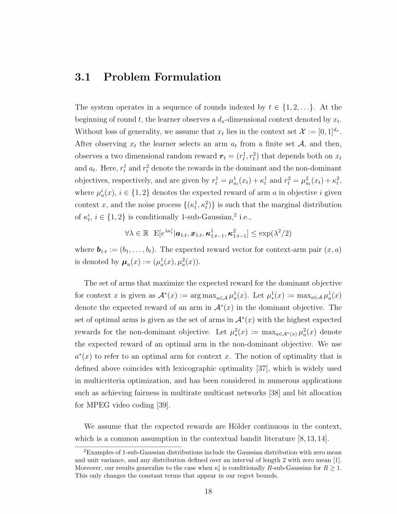
We assume that the expected rewards are Holder continuous in the context,

which is a common assumption in the contextual bandit literature [8, 13,14].

2Examples of 1-sub-Gaussian distributions include the Gaussian distribution with zero meanand unit variance, and any distribution defined over an interval of length 2 with zero mean [1].Moreover, our results generalize to the case when κit is conditionally R-sub-Gaussian for R ≥ 1.This only changes the constant terms that appear in our regret bounds.

18

Assumption 1. There exists L > 0, 0 < α ≤ 1 such that for all i ∈ 1, 2 , a ∈ Aand x, x′ ∈ X , we have

|µia(x)− µia(x′)| < L ‖x− x′‖α .

Since Holder continuity implies continuity, for any nontrivial contextual MAB

in which the sets of optimal arms in the first objective are different for at least

two contexts, there exists at least one context x ∈ X for which A∗(x) is not a

singleton. Let X∗ denote the set of contexts for which A∗(x) is not a singleton.

Since we make no assumptions on how contexts arrive, it is possible that majority

of contexts that arrive by round T are in set X∗. This implies that contextual

MAB algorithms that only aim at maximizing the rewards in the first objective

cannot learn the optimal arms for each context.

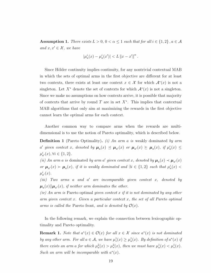
Another common way to compare arms when the rewards are multi-

dimensional is to use the notion of Pareto optimality, which is described below.

Definition 1 (Pareto Optimality). (i) An arm a is weakly dominated by arm

a′ given context x, denoted by µa(x) µa′(x) or µa′(x) µa(x), if µia(x) ≤µia′(x),∀i ∈ 1, 2.(ii) An arm a is dominated by arm a′ given context x, denoted by µa(x) ≺ µa′(x)

or µa′(x) µa(x), if it is weakly dominated and ∃i ∈ 1, 2 such that µia(x) <

µia′(x).

(iii) Two arms a and a′ are incomparable given context x, denoted by

µa(x)||µa′(x), if neither arm dominates the other.

(iv) An arm is Pareto optimal given context x if it is not dominated by any other

arm given context x. Given a particular context x, the set of all Pareto optimal

arms is called the Pareto front, and is denoted by O(x).

In the following remark, we explain the connection between lexicographic op-

timality and Pareto optimality.

Remark 1. Note that a∗(x) ∈ O(x) for all x ∈ X since a∗(x) is not dominated

by any other arm. For all a ∈ A, we have µ1∗(x) ≥ µ1

a(x). By definition of a∗(x) if

there exists an arm a for which µ2a(x) > µ2

∗(x), then we must have µ1a(x) < µ1

∗(x).

Such an arm will be incomparable with a∗(x).

19

3.1.1 Definitions of the 2D Regret and the Pareto Regret

Initially, the learner does not know the expected rewards; it learns them over

time. The goal of the learner is to compete with an oracle, which knows the

expected rewards of the arms for every context and chooses the optimal arm

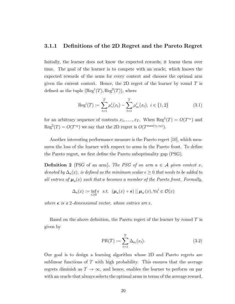
given the current context. Hence, the 2D regret of the learner by round T is

defined as the tuple (Reg1(T ),Reg2(T )), where

Regi(T ) :=T∑t=1

µi∗(xt)−T∑t=1

µiat(xt), i ∈ 1, 2 (3.1)

for an arbitrary sequence of contexts x1, . . . , xT . When Reg1(T ) = O(T γ1) and

Reg2(T ) = O(T γ2) we say that the 2D regret is O(Tmax(γ1,γ2)).

Another interesting performance measure is the Pareto regret [10], which mea-

sures the loss of the learner with respect to arms in the Pareto front. To define

the Pareto regret, we first define the Pareto suboptimality gap (PSG).

Definition 2 (PSG of an arm). The PSG of an arm a ∈ A given context x,

denoted by ∆a(x), is defined as the minimum scalar ε ≥ 0 that needs to be added to

all entries of µa(x) such that a becomes a member of the Pareto front. Formally,

∆a(x) := infε≥0

ε s.t. (µa(x) + ε) || µa′(x),∀a′ ∈ O(x)

where ε is a 2-dimensional vector, whose entries are ε.

Based on the above definition, the Pareto regret of the learner by round T is

given by

PR(T ) :=T∑t=1

∆at(xt). (3.2)

Our goal is to design a learning algorithm whose 2D and Pareto regrets are

sublinear functions of T with high probability. This ensures that the average

regrets diminish as T → ∞, and hence, enables the learner to perform on par

with an oracle that always selects the optimal arms in terms of the average reward.

20

3.1.2 Applications of CMAB-DO

In this subsection we describe four possible applications of CMAB-DO.

3.1.2.1 Multichannel Communication

Consider a multi-channel communication application in which a user chooses a

channel Q ∈ Q and a transmission rate R ∈ R in each round after receiving

context xt := SNRQ,tQ∈Q, where SNRQ,t is the transmit signal to noise ratio of

channel Q in round t. For instance, if each channel is also allocated to a primary

user, then SNRQ,t can change from round to round due to time varying transmit

power constraint in order not to cause outage to the primary user on channel Q.

In this setup, each arm corresponds to a transmission rate-channel pair (R,Q)

denoted by aR,Q. Hence, the set of arms is A = R × Q. When the user com-

pletes its transmission at the end of round t, it receives a 2-dimensional reward

where the dominant one is related to throughput and the non-dominant one is

related to reliability. Here, r2t ∈ 0, 1 where 0 and 1 correspond to failed and

successful transmission, respectively. Moreover, the success rate of aR,Q is equal

to µ2aR,Q

(xt) = 1 − pout(R,Q, xt), where pout(·) denotes the outage probability.

Here, pout(R,Q, xt) also depends on the gain on channel Q whose distribution

is unknown to the user. On the other hand, for aR,Q, r1t ∈ 0, R/Rmax and

µ1aR,Q

(xt) = R(1 − pout(R,Q, xt))/Rmax, where Rmax is the maximum rate. It is

usually the case that the outage probability increases with R, so maximizing the

throughput and reliability are usually conflicting objectives.3 Illustrative results

on this application are given in Section 3.5.

3Note that in this example, given that arm aR,Q is selected, we have κ1t = r1t − µ1aR,Q

(xt)

and κ2t = r2t −µ2aR,Q

(xt). Clearly, both κ1t and κ2t are zero mean with support in [−1, 1]. Hence,

they are 1-sub-Gaussian.

21

3.1.2.2 Online Binary Classification

Consider a medical diagnosis problem where a patient with context xt (including

features such as age, gender, medical test results etc.) arrives in round t. Then,

this patient is assigned to one of the experts inA who will diagnose the patient. In

reality, these experts can either be clinical decision support systems or humans,

but the classification performance of these experts are context dependent and

unknown a priori. In this problem, the dominant objective can correspond to

accuracy while the non-dominant objective can correspond to false negative rate.

For this case, the rewards in both objectives are binary, and depend on whether

the classification is correct and a positive case is correctly identified.

3.1.2.3 Recommender System

Recommender systems involve optimization of multiple metrics like novelty and

diversity in addition to accuracy [40,41]. Below, we describe how a recommender

system with accuracy and diversity metrics can be modeled using CMAB-DO.

At the beginning of round t a user with context xt arrives to the recommender

system. Then, an item from set A is recommended to the user along with a

novelty rating box which the user can use to rate the item as novel or not novel.4

The recommendation is considered to be accurate when the user clicks to the

item, and is considered to be novel when the user rates the item as novel.5 Thus,

r1t = 1 if the user clicks to the item and 0 otherwise. Similarly, r2t = 1 if the user

rates the item as novel and 0 otherwise. The distribution of (r1t , r2t ) depends on

xt and is unknown to the recommender system.

Another closely related application is display advertising [42], where an ad-

vertiser can place an ad to the publisher’s website for the user currently visiting

4An example recommender system that uses this kind of feedback is given in [41].5In reality, it is possible that some users may not provide the novelty rating. These users

can be discarded from the calculation of the regret.

22

the website through a payment mechanism. The goal of the advertiser is to max-

imize its click through rate while keeping the costs incurred through payments

at a low level. Thus, it aims at placing an ad only when the current user with

context xt has positive probability of clicking to the ad. Illustrative results on

this application are given in Section 3.5.

3.1.2.4 Network Routing

Packet routing in a communication network commonly involves multiple paths.

Adaptive packet routing can improve the performance by avoiding congested and

faulty links. In many networking problems, it is desirable to minimize energy

consumption as well as the delay due to the energy constraints of sensor nodes.

For instance, lexicographic optimality is used in [43] to obtain routing flows in a

wireless sensor network with energy limited nodes. Moreover, [44] studies a com-

munication network with elastic and inelastic flows, and proposes load-balancing

and rate-control algorithms that prioritize satisfying the rate demanded by in-

elastic traffic.

Given a source destination pair (src, dst) in an energy constrained wireless

sensor network, we can formulate routing of the flow from node src to node

dst using CMAB-DO. At the beginning of each round, the network manager

observes the network state xt, which can be the normalized round-trip time on

some measurement paths. Then, it selects a path from the set of available paths

A and observes the normalized random energy consumption c1t and delay c2t over

the selected path. These costs are converted to rewards by setting r1t = 1 − c1tand r2t = 1− c2t .

23

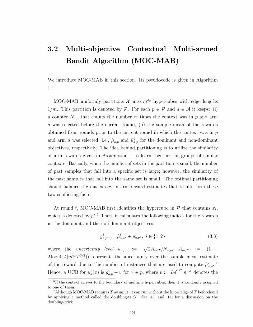
3.2 Multi-objective Contextual Multi-armed

Bandit Algorithm (MOC-MAB)

We introduce MOC-MAB in this section. Its pseudocode is given in Algorithm

1.

MOC-MAB uniformly partitions X into mdx hypercubes with edge lengths

1/m. This partition is denoted by P . For each p ∈ P and a ∈ A it keeps: (i)

a counter Na,p that counts the number of times the context was in p and arm

a was selected before the current round, (ii) the sample mean of the rewards

obtained from rounds prior to the current round in which the context was in p

and arm a was selected, i.e., µ1a,p and µ2

a,p for the dominant and non-dominant

objectives, respectively. The idea behind partitioning is to utilize the similarity

of arm rewards given in Assumption 1 to learn together for groups of similar

contexts. Basically, when the number of sets in the partition is small, the number

of past samples that fall into a specific set is large; however, the similarity of

the past samples that fall into the same set is small. The optimal partitioning

should balance the inaccuracy in arm reward estimates that results form these

two conflicting facts.

At round t, MOC-MAB first identifies the hypercube in P that contains xt,

which is denoted by p∗.6 Then, it calculates the following indices for the rewards

in the dominant and the non-dominant objectives:

gia,p∗ := µia,p∗ + ua,p∗ , i ∈ 1, 2 (3.3)

where the uncertainty level ua,p :=√

2Am,T/Na,p, Am,T := (1 +

2 log(4|A|mdxT 3/2)) represents the uncertainty over the sample mean estimate

of the reward due to the number of instances that are used to compute µia,p∗ .7

Hence, a UCB for µia(x) is gia,p + v for x ∈ p, where v := Ldα/2x m−α denotes the

6If the context arrives to the boundary of multiple hypercubes, then it is randomly assignedto one of them.

7Although MOC-MAB requires T as input, it can run without the knowledge of T beforehandby applying a method called the doubling-trick. See [45] and [14] for a discussion on thedoubling-trick.

24

Algorithm 1 MOC-MAB

1: Input: T , dx, L, α, m, β2: Initialize sets: Create partition P of X into mdx identical hypercubes3: Initialize counters: Na,p = 0, ∀a ∈ A, ∀p ∈ P , t = 14: Initialize estimates: µ1

a,p = µ2a,p = 0, ∀a ∈ A, ∀p ∈ P

5: while 1 ≤ t ≤ T do6: Find p∗ ∈ P such that xt ∈ p∗7: Compute gia,p∗ for a ∈ A, i ∈ 1, 2 as given in (3.3)8: Set a∗1 = arg maxa∈A g

1a,p∗ . (break ties randomly)

9: if ua∗1,p∗ > βv then10: Select arm at = a∗111: else12: Find set of candidate optimal arms A∗ given in (3.4)13: Select arm at = arg maxa∈A∗ g

2a,p∗ (break ties randomly)

14: end if15: Observe rt = (r1t , r

2t )

16: µiat,p∗ ← (µiat,p∗Nat,p∗ + rit)/(Nat,p∗ + 1), i ∈ 1, 217: Nat,p∗ ← Nat,p∗ + 118: t← t+ 119: end while

non-vanishing uncertainty term due to context set partitioning. Since this term

is non-vanishing, we also name it the margin of tolerance. The main learning

principle in such a setting is called optimism under the face of uncertainty. The

idea is to inflate the reward estimates from arms that are not selected often by a

certain level, such that the inflated reward estimate becomes an upper confidence

bound for the true expected reward with a very high probability. This way, arms

that are not selected frequently are explored, and this exploration potentially

helps the learner to discover arms that are better than the arm with the highest

estimated reward. As expected, the uncertainty level vanishes as an arm gets

selected more often.

After calculating the UCBs, MOC-MAB judiciously determines the arm to

select based on these UCBs. It is important to note that the choice a∗1 :=

arg maxa∈A g1a,p∗ can be highly suboptimal for the non-dominant objective. To

see this, consider a very simple setting, where A = a, b, µ1a(x) = µ1

b(x) = 0.5,

µ2a(x) = 1 and µ2

b(x) = 0 for all x ∈ X . For an algorithm that always selects

at = a∗1 and that randomly chooses one of the arms with the highest index in the

25

dominant objective in case of a tie, both arms will be equally selected in expec-

tation. Hence, due to the noisy rewards, there are sample paths in which arm

2 is selected more than half of the time. For these sample paths, the expected

regret in the non-dominant objective is at least T/2. MOC-MAB overcomes the

effect of the noise mentioned above due to the randomness in the rewards and the

partitioning of X by creating a safety margin below the maximal index g1a∗1,p∗ for

the dominant objective, when its confidence for a∗1 is high, i.e., when ua∗1,p∗ ≤ βv,

where β > 0 is a constant. For this, it calculates the set of candidate optimal

arms given as

A∗ :=a ∈ A : g1a,p∗ ≥ µ1

a∗1,p∗ − ua∗1,p∗ − 2v

(3.4)

=a ∈ A : µ1

a,p∗ ≥ µ1a∗1,p

∗ − ua∗1,p∗ − ua,p∗ − 2v.

Here, the term −ua∗1,p∗ − ua,p∗ − 2v accounts for the joint uncertainty over

the sample mean rewards of arms a and a∗1. Then, MOC-MAB selects at =

arg maxa∈A∗ g2a,p∗ .

On the other hand, when its confidence for a∗1 is low, i.e., when ua∗1,p∗ > βv,

it has a little hope even in selecting an optimal arm for the dominant objective.

In this case it just selects at = a∗1 to improve its confidence for a∗1. After its arm

selection, it receives the random reward vector rt, which is then used to update

the counters and the sample mean rewards for p∗.

Remark 2. At each round, finding the set in P that xt belongs to requires O(dx)

computations. Moreover, each of the following processes requires O(|A|) compu-

tations: (i) finding maximum value among the indices of the dominant objective,

(ii) creating a candidate set and finding maximum value among the indices of

the non-dominant objective. Hence, MOC-MAB requires O(dxT )+O(|A|T ) com-

putations in T rounds. In addition, the memory complexity of MOC-MAB is

O(mdx|A|).

Remark 3. MOC-MAB allows the sample mean reward of the selected arm to be

less than the sample mean reward of a∗1 by at most ua∗1,p∗ + ua,p∗ + 2v. Here, 2v

term does not vanish as arms get selected since it results from the partitioning of

the context set. While setting v based on the time horizon allows the learner to

26

control the regret due to partitioning, in some settings having this non-vanishing

term allows MOC-MAB to achieve reward that is much higher than the reward

of the oracle in the non-dominant objective. Such an example is given in Section

3.5.

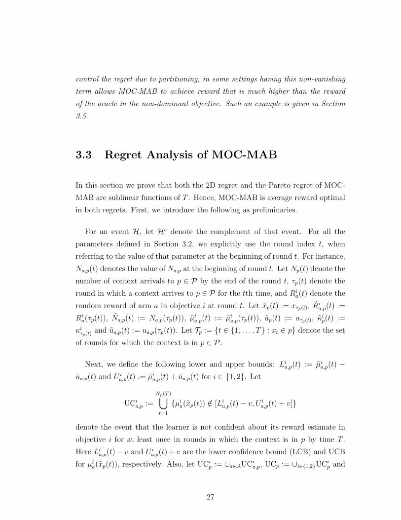
3.3 Regret Analysis of MOC-MAB

In this section we prove that both the 2D regret and the Pareto regret of MOC-

MAB are sublinear functions of T . Hence, MOC-MAB is average reward optimal

in both regrets. First, we introduce the following as preliminaries.

For an event H, let Hc denote the complement of that event. For all the

parameters defined in Section 3.2, we explicitly use the round index t, when

referring to the value of that parameter at the beginning of round t. For instance,

Na,p(t) denotes the value of Na,p at the beginning of round t. Let Np(t) denote the

number of context arrivals to p ∈ P by the end of the round t, τp(t) denote the

round in which a context arrives to p ∈ P for the tth time, and Ria(t) denote the

random reward of arm a in objective i at round t. Let xp(t) := xτp(t), Ria,p(t) :=

Ria(τp(t)), Na,p(t) := Na,p(τp(t)), µ

ia,p(t) := µia,p(τp(t)), ap(t) := aτp(t), κ

ip(t) :=

κiτp(t) and ua,p(t) := ua,p(τp(t)). Let Tp := t ∈ 1, . . . , T : xt ∈ p denote the set

of rounds for which the context is in p ∈ P .

Next, we define the following lower and upper bounds: Lia,p(t) := µia,p(t) −ua,p(t) and U i

a,p(t) := µia,p(t) + ua,p(t) for i ∈ 1, 2. Let

UCia,p :=

Np(T )⋃t=1

µia(xp(t)) /∈ [Lia,p(t)− v, U ia,p(t) + v]

denote the event that the learner is not confident about its reward estimate in

objective i for at least once in rounds in which the context is in p by time T .

Here Lia,p(t)− v and U ia,p(t) + v are the lower confidence bound (LCB) and UCB

for µia(xp(t)), respectively. Also, let UCip := ∪a∈AUCi

a,p, UCp := ∪i∈1,2UCip and

27

UC := ∪p∈PUCp, and for each i ∈ 1, 2, p ∈ P and a ∈ A, let

µia,p = supx∈p

µia(x) and µia,p

= infx∈p

µia(x).

Let

Regip(T ) :=

Np(T )∑t=1

µi∗(xp(t))−Np(T )∑t=1

µiap(t)(xp(t))

denote the regret incurred in objective i for rounds in Tp (regret incurred in

p ∈ P). Then, the total regret in objective i can be written as

Regi(T ) =∑p∈P

Regip(T ). (3.5)

Thus, the expected regret in objective i becomes

E[Regi(T )] =∑p∈P

E[Regip(T )]. (3.6)

In the following analysis, we will bound both Regi(T ) under the event UCc and

E[Regi(T )]. For the latter, we will use the following decomposition:

E[Regip(T )] = E[Regip(T ) | UC] Pr(UC) + E[Regip(T ) | UCc] Pr(UCc)

≤ CimaxNp(T ) Pr(UC) + E[Regip(T ) | UCc] (3.7)

where Cimax is the maximum difference in the expected reward of an optimal arm

and any other arm for objective i.

Having obtained the decomposition in (3.7), we proceed by bounding the terms

in (3.7). For this, we first bound Pr(UCp) in the next lemma.

Lemma 1. For any p ∈ P, we have Pr(UCp) ≤ 1/(mdxT ).

Proof. From the definitions of Lia,p(t), Uia,p(t) and UCi

a,p, it can be observed that

the event UCia,p happens when µia(xp(t)) does not fall into the confidence interval

[Lia,p(t) − v, U ia,p(t) + v] for some t. The probability of this event could be eas-

ily bounded by using the concentration inequality given in Appendix A, if the

28

expected reward from the same arm did not change over rounds. However, this

is not the case in our model since the elements of xp(t)Np(T )t=1 are not identical

which makes the distributions of Ria,p(t), t ∈ 1, . . . , Np(T ) different.

In order to resolve this issue, we propose the following: Recall that

Ria,p(t) = µia(xp(t)) + κip(t)

and

µia,p(t) =

∑t−1l=1 R

ia,p(l)I(ap(l) = a)

Na,p(t).

when Na,p(t) > 0. Note that when Na,p(t) = 0, we have µia,p(t) = 0. We define

two new sequences of random variables, whose sample mean values will lower and

upper bound µia,p(t). The best sequence is defined as Ri

a,p(t)Np(T )t=1 where

Ri

a,p(t) = µia,p + κip(t)

and the worst sequence is defined as Ria,p(t)

Np(T )t=1 where

Ria,p(t) = µi

a,p+ κip(t).

Let

µia,p(t) :=t−1∑l=1

Ri

a,p(l)I(ap(l) = a)/Na,p(t)

µia,p

(t) :=t−1∑l=1

Ria,p(l)I(ap(l) = a)/Na,p(t).

for Na,p(t) > 0 and µia,p(t) = µia,p

(t) = 0 for Na,p(t) = 0.

We have

µia,p

(t) ≤ µia,p(t) ≤ µia,p(t) ∀t ∈ 1, . . . , Np(T )

almost surely.

Let

Li

a,p(t) := µia,p(t)− ua,p(t)

29

Ui

a,p(t) := µia,p(t) + ua,p(t)

Lia,p(t) := µia,p

(t)− ua,p(t)

U ia,p(t) := µi

a,p(t) + ua,p(t).

Note that Pr(µia(xp(t)) /∈ [Lia,p(t) − v, U ia,p(t) + v]) = 0 for Na,p(t) = 0 since we

have Lia,p(t) = −∞ and U ia,p(t) = +∞ when Na,p(t) = 0. Thus, in the rest of the

proof, we focus on the case when Na,p(t) > 0. It can be shown that

µia(xp(t)) /∈ [Lia,p(t)− v, U ia,p(t) + v] ⊂ µia(xp(t)) /∈ [L

i

a,p(t)− v, Ui

a,p(t) + v]

∪ µia(xp(t)) /∈ [Lia,p(t)− v, U ia,p(t) + v].

(3.8)

The following inequalities can be obtained from the Holder continuity assumption:

µia(xp(t)) ≤ µia,p ≤ µia(xp(t)) + L

(√dxm

)α(3.9)

µia(xp(t))− L(√

dxm

)α≤ µi

a,p≤ µia(xp(t)). (3.10)

Since v = L(√

dx/m)α

, using (3.9) and (3.10) it can be shown that

(i) µia(xp(t)) /∈[Li

a,p(t)− v, Ui

a,p(t) + v] ⊂ µia,p /∈ [Li

a,p(t), Ui

a,p(t)],

(ii) µia(xp(t)) /∈[Lia,p(t)− v, U ia,p(t) + v] ⊂ µi

a,p/∈ [Lia,p(t), U

ia,p(t)].

Plugging these into (3.8), we get

µia(xp(t)) /∈ [Lia,p(t)− v, U ia,p(t) + v]

⊂ µia,p /∈ [Li

a,p(t), Ui

a,p(t)] ∪ µia,p /∈ [Lia,p(t), Uia,p(t)].

Then, using the equation above and the union bound, we obtain

Pr(UCia,p) ≤ Pr

Np(T )⋃t=1

µia,p /∈ [Li

a,p(t), Ui

a,p(t)]

+ Pr

Np(T )⋃t=1

µia,p

/∈ [Lia,p(t), Uia,p(t)]

.

30

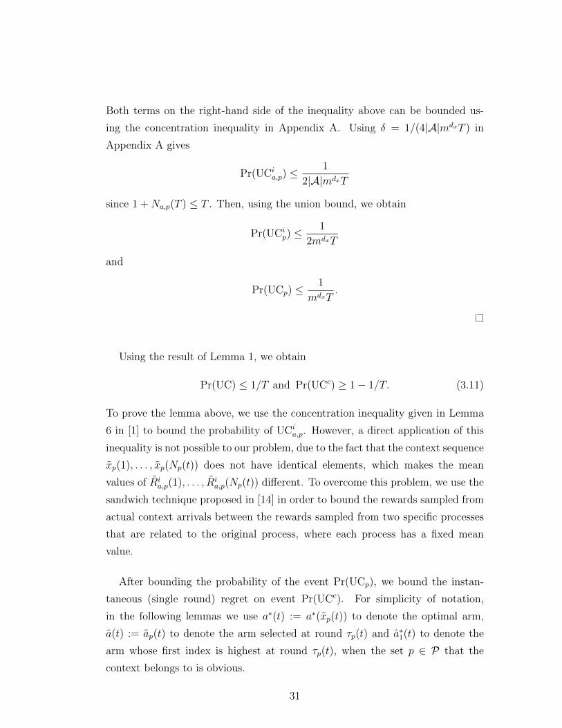
Both terms on the right-hand side of the inequality above can be bounded us-

ing the concentration inequality in Appendix A. Using δ = 1/(4|A|mdxT ) in

Appendix A gives

Pr(UCia,p) ≤

1

2|A|mdxT

since 1 +Na,p(T ) ≤ T . Then, using the union bound, we obtain

Pr(UCip) ≤

1

2mdxT

and

Pr(UCp) ≤1

mdxT.

Using the result of Lemma 1, we obtain

Pr(UC) ≤ 1/T and Pr(UCc) ≥ 1− 1/T. (3.11)

To prove the lemma above, we use the concentration inequality given in Lemma

6 in [1] to bound the probability of UCia,p. However, a direct application of this

inequality is not possible to our problem, due to the fact that the context sequence

xp(1), . . . , xp(Np(t)) does not have identical elements, which makes the mean

values of Ria,p(1), . . . , Ri

a,p(Np(t)) different. To overcome this problem, we use the

sandwich technique proposed in [14] in order to bound the rewards sampled from

actual context arrivals between the rewards sampled from two specific processes

that are related to the original process, where each process has a fixed mean

value.

After bounding the probability of the event Pr(UCp), we bound the instan-

taneous (single round) regret on event Pr(UCc). For simplicity of notation,

in the following lemmas we use a∗(t) := a∗(xp(t)) to denote the optimal arm,

a(t) := ap(t) to denote the arm selected at round τp(t) and a∗1(t) to denote the

arm whose first index is highest at round τp(t), when the set p ∈ P that the

context belongs to is obvious.

31

The following lemma shows that on event UCcp the regret incurred in a round

τp(t) for the dominant objective can be bounded as function of the difference

between the upper and lower confidence bounds plus the margin of tolerance.

Lemma 2. When MOC-MAB is run, on event UCcp, we have

µ1a∗(t)(xp(t))− µ1

a(t)(xp(t)) ≤ U1a(t),p(t)− L1

a(t),p(t) + 2(β + 2)v

for all t ∈ 1, . . . , Np(T ).

Proof. We consider two cases. When ua∗1(t),p(t) ≤ βv, we have

U1a(t),p(t) ≥ L1

a∗1(t),p(t)− 2v ≥ U1

a∗1(t),p(t)− 2ua∗1(t),p(t)− 2v

≥ U1a∗1(t),p

(t)− 2(β + 1)v.

On the other hand, when ua∗1(t),p(t) > βv, the selected arm is a(t) = a∗1(t). Hence,

we obtain

U1a(t),p(t) = U1

a∗1(t),p(t) ≥ U1

a∗1(t),p(t)− 2(β + 1)v.

Thus, for both cases, we have

U1a(t),p(t) ≥ U1

a∗1(t),p(t)− 2(β + 1)v (3.12)

and

U1a∗1(t),p

(t) ≥ U1a∗(t),p(t). (3.13)

On event UCcp, we also have

µ1a∗(t)(xp(t)) ≤ U1

a∗(t),p(t) + v (3.14)

and

µ1a(t)(xp(t)) ≥ L1

a(t),p(t)− v. (3.15)

By combining (3.12)-(3.15), we obtain

µ1a∗(t)(xp(t))− µ1

a(t)(xp(t)) ≤ U1a(t),p(t)− L1

a(t),p(t) + 2(β + 2)v.

32

The lemma below bounds the regret incurred in a round τp(t) for the non-

dominant objective on event UCcp when the uncertainty level of the arm with the

highest index in the dominant objective is low.

Lemma 3. When MOC-MAB is run, on event UCcp, for t ∈ 1, . . . , Np(T ) if

ua∗1(t),p(t) ≤ βv

holds, then we have

µ2a∗(t)(xp(t))− µ2

a(t)(xp(t)) ≤ U2a(t),p(t)− L2

a(t),p + 2v.

Proof. When ua∗1(t),p(t) ≤ βv holds, all arms that are selected as candidate optimal

arms have their index for objective 1 in the interval [L1a∗1(t),p

(t) − 2v, U1a∗1(t),p

(t)].

Next, we show that U1a∗(t),p(t) is also in this interval.

On event UCcp, we have

µ1a∗(t)(xp(t)) ∈ [L1

a∗(t),p(t)− v, U1a∗(t),p(t) + v]

µ1a∗1(t)

(xp(t)) ∈ [L1a∗1(t),p

(t)− v, U1a∗1(t),p

(t) + v].

We also know that

µ1a∗(t)(xp(t)) ≥ µ1

a∗1(t)(xp(t)).

Using the inequalities above, we obtain

U1a∗(t),p(t) ≥ µ1

a∗(t)(xp(t))− v ≥ µ1a∗1(t)

(xp(t))− v ≥ L1a∗1(t),p

(t)− 2v.

Since the selected arm has the maximum index for the non-dominant objective

among all arms whose indices for the dominant objective are in [L1a∗1(t),p

(t) −2v, U1

a∗1(t),p(t)], we have U2

a(t),p(t) ≥ U2a∗(t),p(t). Combining this with the fact that

UCcp holds, we get

µ2a(t)(xp(t)) ≥ L2

a(t),p(t)− v (3.16)

and

µ2a∗(t)(xp(t)) ≤ U2

a∗(t),p(t) + v ≤ U2a(t),p(t) + v. (3.17)

33

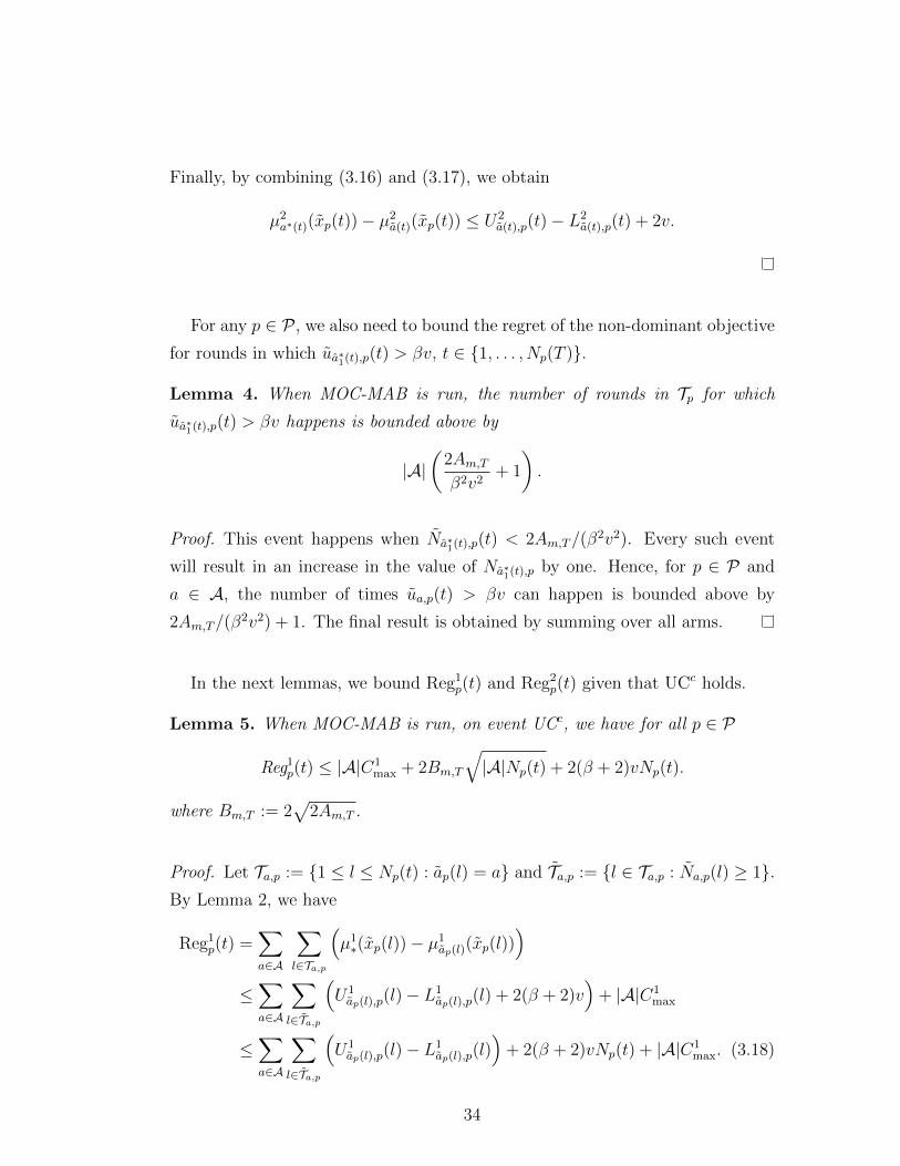
Finally, by combining (3.16) and (3.17), we obtain

µ2a∗(t)(xp(t))− µ2

a(t)(xp(t)) ≤ U2a(t),p(t)− L2

a(t),p(t) + 2v.

For any p ∈ P , we also need to bound the regret of the non-dominant objective

for rounds in which ua∗1(t),p(t) > βv, t ∈ 1, . . . , Np(T ).

Lemma 4. When MOC-MAB is run, the number of rounds in Tp for which

ua∗1(t),p(t) > βv happens is bounded above by

|A|(

2Am,Tβ2v2

+ 1

).

Proof. This event happens when Na∗1(t),p(t) < 2Am,T/(β

2v2). Every such event

will result in an increase in the value of Na∗1(t),pby one. Hence, for p ∈ P and

a ∈ A, the number of times ua,p(t) > βv can happen is bounded above by

2Am,T/(β2v2) + 1. The final result is obtained by summing over all arms.

In the next lemmas, we bound Reg1p(t) and Reg2

p(t) given that UCc holds.

Lemma 5. When MOC-MAB is run, on event UCc, we have for all p ∈ P

Reg1p(t) ≤ |A|C1max + 2Bm,T

√|A|Np(t) + 2(β + 2)vNp(t).

where Bm,T := 2√

2Am,T .

Proof. Let Ta,p := 1 ≤ l ≤ Np(t) : ap(l) = a and Ta,p := l ∈ Ta,p : Na,p(l) ≥ 1.By Lemma 2, we have

Reg1p(t) =

∑a∈A

∑l∈Ta,p

(µ1∗(xp(l))− µ1

ap(l)(xp(l)))

≤∑a∈A

∑l∈Ta,p

(U1ap(l),p(l)− L

1ap(l),p(l) + 2(β + 2)v

)+ |A|C1

max

≤∑a∈A

∑l∈Ta,p

(U1ap(l),p(l)− L

1ap(l),p(l)

)+ 2(β + 2)vNp(t) + |A|C1

max. (3.18)

34

We also have

∑a∈A

∑l∈Ta,p

(U1ap(l),p(l)− L

1ap(l),p(l)

)≤∑a∈A

Bm,T

∑l∈Ta,p

√1

Na,p(l)

≤ Bm,T

∑a∈A

Na,p(t)−1∑k=0

√1

1 + k

≤ 2Bm,T

∑a∈A

√Na,p(t) (3.19)

≤ 2Bm,T

√|A|Np(t) (3.20)

where Bm,T = 2√

2Am,T , and (3.19) follows from the fact that

Na,p(t)−1∑k=0

√1

1 + k≤∫ Na,p(t)

x=0

1√xdx = 2

√Na,p(t).

Combining (3.18) and (3.20), we obtain that on event UCc

Reg1p(t) ≤ |A|C1

max + 2Bm,T

√|A|Np(t) + 2(β + 2)vNp(t).

Lemma 6. When MOC-MAB is run, on event UCc we have for all p ∈ P

Reg2p(t) ≤ C2max|A|

(2Am,Tβ2v2

+ 1

)+ 2vNp(t) + 2Bm,T

√|A|Np(t).

Proof. Using the result of Lemma 4, the contribution to the regret of the non-

dominant objective in rounds for which ua∗1(t),p(t) > βv is bounded by

C2max|A|

(2Am,Tβ2v2

+ 1

). (3.21)

Let T 2a,p := l ≤ Np(t) : ap(l) = a and Na,p(l) ≥ 2Am,T/(β

2v2). By Lemma 3,

we have∑a∈A

∑l∈T 2

a,p

(µ2∗(xp(l))− µ2

ap(l)(xp(l)))≤∑a∈A

∑l∈T 2

a,p

(U2ap(l),p(l)− L

2ap(l),p(l) + 2v

)=∑a∈A

∑l∈T 2

a,p

(U2ap(l),p(l)− L

2ap(l),p(l)

)+ 2vNp(t)

(3.22)

35

We have on event UCc

∑a∈A

∑l∈T 2

a,p

(U2ap(l),p(l)− L

2ap(l),p(l)

)≤∑a∈A

Bm,T

∑l∈T 2

a,p

√1

Na,p(l)

≤ Bm,T

∑a∈A

Na,p(t)−1∑k=0

√1

1 + k

≤ 2Bm,T

∑a∈A

√Na,p(t)

≤ 2Bm,T

√|A|Np(t). (3.23)

where Bm,T = 2√

2Am,T . Combining (3.21), (3.22) and (3.23), we obtain

Reg2p(t) ≤ C2

max|A|(

2Am,Tβ2v2

+ 1

)+ 2vNp(t) + 2Bm,T

√|A|Np(t).

Next, we use the result of Lemmas 1, 5 and 6 to find a bound on Regi(t) that

holds for all t ≤ T with probability at least 1− 1/T .

Theorem 1. When MOC-MAB is run, we have for any i ∈ 1, 2

Pr(Regi(t) < εi(t) ∀t ∈ 1, . . . , T) ≥ 1− 1/T

where

ε1(t) = mdx|A|C1max + 2Bm,T

√|A|mdxt+ 2(β + 2)vt

and

ε2(t) = mdx|A|C2max +mdxC2

max|A|(

2Am,Tβ2v2

)+ 2Bm,T

√|A|mdxt+ 2vt.

Proof. By (3.5) and Lemmas 5 and 6, we have on event UCc:

Reg1(t) ≤mdx|A|C1max + 2Bm,T

∑p∈P

√|A|Np(t) + 2(β + 2)vt

≤mdx|A|C1max + 2Bm,T

√|A|mdxt+ 2(β + 2)vt.

36

and

Reg2(t) ≤mdx |A|C2max +mdxC2

max|A|(

2Am,Tβ2v2

)+ 2Bm,T

∑p∈P

√|A|Np(t) + 2vt

≤mdx |A|C2max +mdxC2

max|A|(

2Am,Tβ2v2

)+ 2Bm,T

√|A|mdxt+ 2vt

for all t ≤ T . The result follows from the fact that UCc holds with probability at

least 1− 1/T .

The following theorem shows that the expected 2D regret of MOC-MAB by

time T is O(T2α+dx3α+dx ).

Theorem 2. When MOC-MAB is run with inputs m = dT 1/(3α+dx)e and β > 0,

we have

E[Reg1(T )] ≤C1max + 2dx|A|C1

maxTdx

3α+dx + 2(β + 2)Ldα/2x T2α+dx3α+dx

+2dx/2+1Bm,T

√|A|T

1.5α+dx3α+dx

and

E[Reg2(T )] ≤ 2dx/2+1Bm,T

√|A|T

1.5α+dx3α+dx + C2

max + 2dxC2max|A|T

dx3α+dx

+

(2Ldα/2x +

C2max|A|21+2α+dxAm,T

β2L2dαx

)T

2α+dx3α+dx .

Proof. E[Regi(T )] is bounded by using the result of Theorem 1 and (3.7):

E[Regi(T )] ≤ E[Regi(T ) | UCc] +∑p∈P

CimaxNp(T ) Pr(UC)

≤ E[Regi(T ) | UCc] +∑p∈P

CimaxNp(T )/T

= E[Regi(T ) | UCc] + Cimax.

Therefore, we have

E[Reg1(T )] ≤ ε1(T ) + C1max

E[Reg2(T )] ≤ ε2(T ) + C2max.

37

It can be shown that when we set m = dT 1/(2α+dx)e regret bound of the dominant

objective becomes O(T (α+dx)/(2α+dx)) and regret bound of the non-dominant ob-

jective becomes O(T ). The optimal value for m that makes both regrets sublinear

is m = dT 1/(3α+dx)e. With this value of m, we obtain

E[Reg1(T )] ≤2dx|A|C1maxT

dx3α+dx + 2(β + 2)Ldα/2x T

2α+dx3α+dx

+ 2dx/2+1Bm,T

√|A|T

1.5α+dx3α+dx + C1

max

and

E[Reg2(T )] ≤(

2Ldα/2x +C2

max|A|21+2α+dxAm,Tβ2L2dαx

)T

2α+dx3α+dx

+ C2max + 2dxC2

max|A|Tdx

3α+dx

+ 2dx/2+1Bm,T

√|A|T

1.5α+dx3α+dx .

From the results above we conclude that both regrets are O(T (2α+dx)/(3α+dx)),

where for the first regret bound the constant that multiplies the highest order of

the regret does not depend on A, while the dependence on this term is linear for

the second regret bound.

Next, we show that the expected value of the Pareto regret of MOC-MAB

given in (3.2) is also O(T (2α+dx)/(3α+dx)).

Theorem 3. When MOC-MAB is run with inputs m = dT 1/(3α+dx)e and β > 0,

we have

Pr(PR(t) < ε1(t) ∀t ∈ 1, . . . , T) ≥ 1− 1/T

where ε1(t) is given in Theorem 1 and

E[PR(T )] ≤C1max + 2dx|A|C1

maxTdx

3α+dx + 2(β + 2)Ldα/2x T2α+dx3α+dx

+ 2dx/2+1Bm,T

√|A|T

1.5α+dx3α+dx .

Proof. Consider any p ∈ P and t ∈ 1, . . . , Np(T ). By definition ∆a(t)(xp(t)) ≤µ1a∗(t)(xp(t))− µ1

a(t)(xp(t)). This holds since for any ε > 0, adding µ1a∗(t)(xp(t))−

38

µ1a(t)(xp(t))+ε to µ1

a(t)(xp(t)) will either make it (i) dominate the arms in O(xp(t))

or (ii) incomparable with the arms in O(xp(t)). Hence, using the result in Lemma

2, we have on event UCc

∆a(t)(xp(t)) ≤ U1a(t),p(t)− L1

a(t),p(t) + 2(β + 2)v.

Let PRp(T ) :=∑Np(T )

t=1 ∆a(t)(xp(t)). Hence, PR(T ) =∑

p∈P PRp(T ). Due to this,

the results derived for Reg1(t) and Reg1(T ) in Theorems 1 and 2 also hold for

PRp(t) and PRp(T ).

Theorem 3 shows that the regret measures E[Reg1(T )], E[Reg2(T )] and

E[PR(T )] for MOC-MAB are all O(T (2α+dx)/(3α+dx)) when it is run with m =

dT 1/(3α+dx)e. This implies that MOC-MAB is average reward optimal in all re-

gret measures as T → ∞. The growth rate of the Pareto regret can be fur-

ther decreased by setting m = dT 1/(2α+dx)e. This will make the Pareto regret

O(T (α+dx)/(2α+dx)) (which matches with the lower bound in [8] for the single-

objective contextual MAB with similarity information up to a logaritmic factor)

but will also make the regret in the non-dominant objective linear.

3.4 Extensions

3.4.1 Learning Under Periodically Changing Reward Dis-

tributions

In many practical cases, the reward distribution of an arm changes periodically

over time even under the same context. For instance, in a recommender system

the probability that a user clicks to an ad may change with the time of the day,

but the pattern of change can be periodical on a daily basis and this can be

known by the system. Moreover, this change is usually gradual over time. In this

section, we extend MOC-MAB such that it can deal with such settings.

For this, let Ts denote the period. For the dx-dimensional context xt =

39

(x1,t, x2,t, ..., xdx,t) received at round t let xt := (x1,t, x2,t, ..., xdx+1,t) denote the

extended context where xdx+1,t := (t mod Ts)/Ts is the time context. Let Xdenote the dx + 1 dimensional extended context set constructed by adding the

time dimension to X . It is assumed that the following holds for the extended

contexts.

Assumption 2. Given any x, x′ ∈ X , there exists L > 0 and 0 < α ≤ 1 such

that for all i ∈ 1, 2 and a ∈ A, we have

|µia(x)− µia(x′)| ≤ L||x− x′||α.

Note that Assumption 2 implies Assumption 1 with L = L and α = α

when xdx+1 = x′dx+1. Moreover, for two contexts (x1, . . . , xdx , xdx+1) and

(x1, . . . , xdx , x′dx+1), we have

|µia(x)− µia(x′)| ≤ L|xdx+1 − x′dx+1|α

which implies that the change in the expected rewards is gradual. Under As-

sumption 2, the performance of MOC-MAB is bounded as follows.

Corollary 1. When MOC-MAB is run with inputs L, α, m = dT 1/(3α+dx+1)e,and β > 0 by using the extended context set X instead of the original context set

X , we have

E[Regi(T )] = O(T (2α+dx+1)/(3α+dx+1)) for i ∈ 1, 2.

Proof. The proof simply follows from the proof of Theorem 2 by extending the

dimension of the context set by one.

3.4.2 Lexicographic Optimality for dr > 2 Objectives

Our problem formulation can be generalized to handle dr > 2 objectives as

follows. Let rt := (r1t , . . . , rdrt ) denote the reward vector in round t and

µa(x) := (µ1a(x), . . . , µdra (x)) denote the expected reward vector for context-arm

40

pair (x, a). We say that arm a lexicographically dominates arm a′ in the first j

objectives for context x, denoted by µa(x) >lex,j µa′(x) if µia(x) > µia′(x), where

i := min k ≤ j : µka(x) 6= µka′(x).8 Then, arm a is defined to be lexicographically

optimal for context x if there is no other arm that lexicographically dominates it

in dr objectives.

Let µi∗(x) denote the expected reward of a lexicographically optimal arm for

context x in objective i. Then, the dr-dimensional regret is defined as follows:

Reg(T ) := (Reg1(T ), . . . ,Regdr(T )) where

Regi(T ) :=T∑t=1

µi∗(xt)−T∑t=1

µiat(xt), i ∈ 1, . . . , dr.

Generalizing MOC-MAB to achieve sublinear regret for all objectives will re-

quire construction of a hierarchy of candidate optimal arm sets similar to the

one given in 3.4. We leave this interesting research problem as future work,

and explain when lexicographically optimality in the first two objectives indi-

cates lexicographic optimality in dr objectives and why the number of cases in

which lexicographically optimality in the first two objectives does not indicate

lexicographic optimality in dr objectives is scarce.

Let A∗j(x) denote the set of lexicographically optimal arms for context x in the

first j objectives. We call the case A∗2(x) = A∗dr(x) for all x ∈ X the degenerate

case of the dr-objective contextual MAB. Similarly, we call the case when there

exists some x ∈ X , for which A∗2(x) 6= A∗dr(x) as the non-degenerate case of

the dr-objective contextual MAB. Next, we argue that non-degenerate case is

uncommon. Since A∗j(x) ⊇ A∗j+1(x) for j ∈ 1, . . . , dr − 1 and there is at least

one lexicographically optimal arm, A∗2(x) 6= A∗dr(x) implies that A∗2(x) is not a

singleton. This implies existence of two arms a and b such that µ1a(x) = µ1

b(x)

and µ2a(x) = µ2

b(x). In contrast, for the contextual MAB to be non-trivial, we

only require existence of at least one context x ∈ X and arms a and b such that

µ1a(x) = µ1

b(x).

8If i does not exist then µka(x) = µk

a′(x) for all k ∈ 1, . . . , j, and hence, arm a does notlexicographically dominate arm a′ in the first j objectives.

41

3.5 Illustrative Results

In order to evaluate the performance of MOC-MAB, we run three different ex-

periments both with synthetic and real-world datasets.

We compare MOC-MAB with the following MAB algorithms:

Pareto UCB1 (P-UCB1): This is the Empirical Pareto UCB1 algorithm pro-

posed in [10].

Scalarized UCB1 (S-UCB1): This is the Scalarized Multi-objective UCB1

algorithm proposed in [10].

Contextual Pareto UCB1 (CP-UCB1): This is the contextual version of

P-UCB1 which partitions the context set in the same way as MOC-MAB does,

and uses a different instance of P-UCB1 in each set of the partition.

Contextual Scalarized UCB1 (CS-UCB1): This is the contextual version of

S-UCB1, which partitions the context set in the same way as MOC-MAB does,

and uses a different instance of S-UCB1 in each set of the partition.

Contextual Dominant UCB1 (CD-UCB1): This is the contextual version of

UCB1 [25], which partitions the context set in the same way as MOC-MAB does,

and uses a different instance of UCB1 in each set of the partition. This algorithm

only uses the rewards from the dominant objective to update the indices of the

arms.

For S-UCB1 and CS-UCB1, the weights of the linear scalarization functions

are chosen as [1, 0], [0.5, 0.5] and [0, 1]. For all contextual algorithms, the par-

tition of the context set is formed by choosing m according to Theorem 2, and

L and α are taken as 1. For MOC-MAB, β is chosen as 1 unless stated oth-

erwise. In addition, we scaled down the uncertainty level (also known as the

confidence term or the inflation term) of all the algorithms by a constant chosen

from 1, 1/5, 1/10, 1/15, 1/20, 1/25, 1/30, since we observed that the regrets of

all algorithms in the dominant objective may become smaller when the uncer-

tainty level is scaled down. The reported results correspond to runs performed

using the optimal scale factor for each experiment.

42

3.5.1 Experiment 1 - Synthetic Dataset

In this experiment, we compare MOC-MAB with other MAB algorithms on a

synthetic multi-objective dataset. We take X = [0, 1]2 and assume that the

context at each round is chosen uniformly at random from X . We consider 4 arms

and the time horizon is set as T = 105. The expected arm rewards for 3 of the

arms are generated as follows: We generate 3 multivariate Gaussian distributions

for the dominant objective and 3 multivariate Gaussian distributions for the non-

dominant objective. For the dominant objective, the mean vectors of the first two

distributions are set as [0.3, 0.5], and the mean vector of the third distribution is

set as [0.7, 0.5]. Similarly, for the non-dominant objective, the mean vectors of the

distributions are set as [0.3, 0.7], [0.3, 0.3] and [0.7, 0.5], respectively. For all the

Gaussian distributions the covariance matrix is given by 0.3∗ I where I is the 2 by

2 identity matrix. Then, each Gaussian distribution is normalized by multiplying

it with a constant, such that its maximum value becomes 1. These normalized

distributions form the expected arm rewards. In addition, the expected reward

of the fourth arm for the dominant objective is set as 0, and its expected reward

for the non-dominant objective is set as the normalized multivariate Gaussian

distribution with mean vector [0.7, 0.5]. We assume that the reward of an arm in

an objective given a context x is a Bernoulli random variable whose parameter is

equal to the magnitude of the corresponding normalized distribution at context

x.

Every algorithm is run 100 times and the results are averaged over these runs.

Simulation results given in Fig. 3.1 show the change in the regret of the al-

gorithms in both objectives as a function of time (rounds). As observed from

the results, MOC-MAB beats all other algorithms in both objectives except CD-

UCB1. While the regret of CD-UCB1 in the dominant objective is slightly better

than that of MOC-MAB, its regret is much worse than MOC-MAB in the non-

dominant objective. This is expected since it only aims to maximize the reward

in the dominant objective without considering the other objective.

43

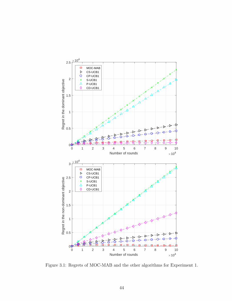
0 1 2 3 4 5 6 7 8 9 10

Number of rounds 104

0

0.5

1

1.5

2

2.5R

egre

t in

the

dom

inan

t obj

ectiv

e104

MOC-MABCS-UCB1CP-UCB1S-UCB1P-UCB1CD-UCB1

0 1 2 3 4 5 6 7 8 9 10

Number of rounds 104

0

0.5

1

1.5

2

2.5

3

Reg

ret i

n th

e no

n-do

min

ant o

bjec

tive

104

MOC-MABCS-UCB1CP-UCB1S-UCB1P-UCB1CD-UCB1

Figure 3.1: Regrets of MOC-MAB and the other algorithms for Experiment 1.

44

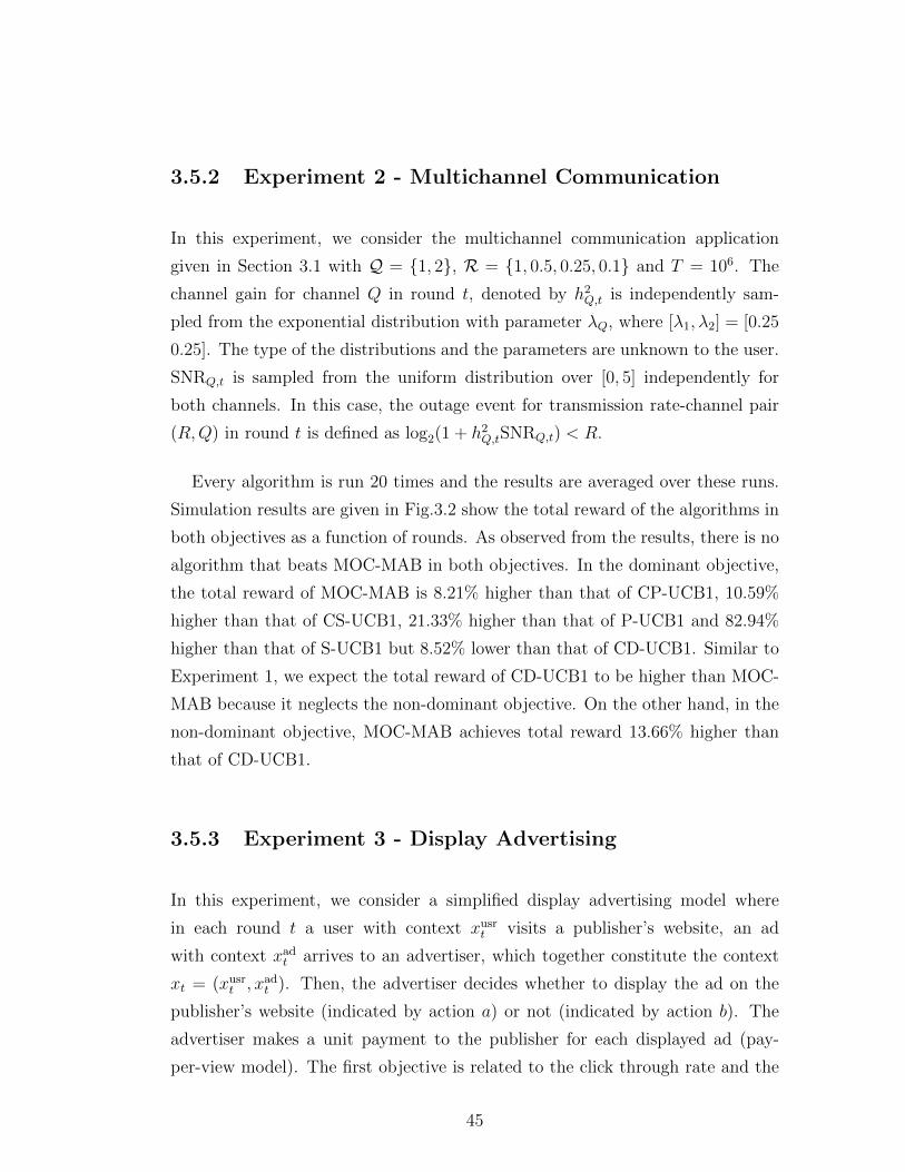
3.5.2 Experiment 2 - Multichannel Communication

In this experiment, we consider the multichannel communication application

given in Section 3.1 with Q = 1, 2, R = 1, 0.5, 0.25, 0.1 and T = 106. The

channel gain for channel Q in round t, denoted by h2Q,t is independently sam-

pled from the exponential distribution with parameter λQ, where [λ1, λ2] = [0.25

0.25]. The type of the distributions and the parameters are unknown to the user.

SNRQ,t is sampled from the uniform distribution over [0, 5] independently for

both channels. In this case, the outage event for transmission rate-channel pair

(R,Q) in round t is defined as log2(1 + h2Q,tSNRQ,t) < R.

Every algorithm is run 20 times and the results are averaged over these runs.

Simulation results are given in Fig.3.2 show the total reward of the algorithms in

both objectives as a function of rounds. As observed from the results, there is no

algorithm that beats MOC-MAB in both objectives. In the dominant objective,

the total reward of MOC-MAB is 8.21% higher than that of CP-UCB1, 10.59%

higher than that of CS-UCB1, 21.33% higher than that of P-UCB1 and 82.94%

higher than that of S-UCB1 but 8.52% lower than that of CD-UCB1. Similar to

Experiment 1, we expect the total reward of CD-UCB1 to be higher than MOC-

MAB because it neglects the non-dominant objective. On the other hand, in the

non-dominant objective, MOC-MAB achieves total reward 13.66% higher than

that of CD-UCB1.

3.5.3 Experiment 3 - Display Advertising

In this experiment, we consider a simplified display advertising model where

in each round t a user with context xusrt visits a publisher’s website, an ad

with context xadt arrives to an advertiser, which together constitute the context

xt = (xusrt , xadt ). Then, the advertiser decides whether to display the ad on the

publisher’s website (indicated by action a) or not (indicated by action b). The

advertiser makes a unit payment to the publisher for each displayed ad (pay-

per-view model). The first objective is related to the click through rate and the

45

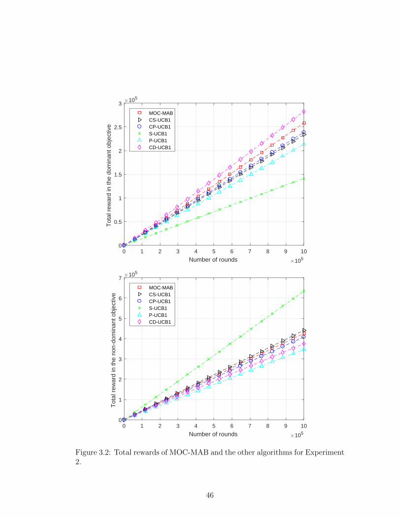
0 1 2 3 4 5 6 7 8 9 10

Number of rounds 105

0

0.5

1

1.5

2

2.5

3T

otal

rew

ard

in th

e do

min

ant o

bjec

tive

105

MOC-MABCS-UCB1CP-UCB1S-UCB1P-UCB1CD-UCB1

0 1 2 3 4 5 6 7 8 9 10

Number of rounds 105

0

1

2

3

4

5

6

7

Tot

al r

ewar

d in

the

non-

dom

inan

t obj

ectiv

e

105

MOC-MABCS-UCB1CP-UCB1S-UCB1P-UCB1CD-UCB1

Figure 3.2: Total rewards of MOC-MAB and the other algorithms for Experiment2.

46

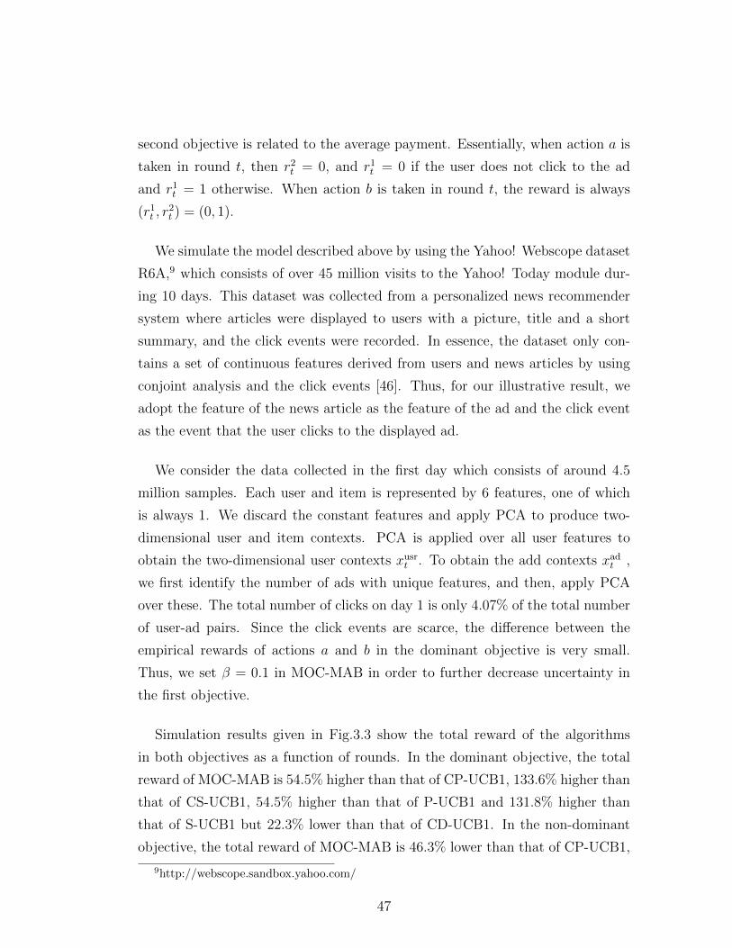
second objective is related to the average payment. Essentially, when action a is

taken in round t, then r2t = 0, and r1t = 0 if the user does not click to the ad

and r1t = 1 otherwise. When action b is taken in round t, the reward is always

(r1t , r2t ) = (0, 1).

We simulate the model described above by using the Yahoo! Webscope dataset

R6A,9 which consists of over 45 million visits to the Yahoo! Today module dur-

ing 10 days. This dataset was collected from a personalized news recommender

system where articles were displayed to users with a picture, title and a short

summary, and the click events were recorded. In essence, the dataset only con-

tains a set of continuous features derived from users and news articles by using

conjoint analysis and the click events [46]. Thus, for our illustrative result, we

adopt the feature of the news article as the feature of the ad and the click event

as the event that the user clicks to the displayed ad.

We consider the data collected in the first day which consists of around 4.5

million samples. Each user and item is represented by 6 features, one of which

is always 1. We discard the constant features and apply PCA to produce two-

dimensional user and item contexts. PCA is applied over all user features to

obtain the two-dimensional user contexts xusrt . To obtain the add contexts xadt ,

we first identify the number of ads with unique features, and then, apply PCA

over these. The total number of clicks on day 1 is only 4.07% of the total number

of user-ad pairs. Since the click events are scarce, the difference between the

empirical rewards of actions a and b in the dominant objective is very small.

Thus, we set β = 0.1 in MOC-MAB in order to further decrease uncertainty in

the first objective.

Simulation results given in Fig.3.3 show the total reward of the algorithms

in both objectives as a function of rounds. In the dominant objective, the total

reward of MOC-MAB is 54.5% higher than that of CP-UCB1, 133.6% higher than

that of CS-UCB1, 54.5% higher than that of P-UCB1 and 131.8% higher than

that of S-UCB1 but 22.3% lower than that of CD-UCB1. In the non-dominant

objective, the total reward of MOC-MAB is 46.3% lower than that of CP-UCB1,

9http://webscope.sandbox.yahoo.com/

47

60% lower than that of CS-UCB1, 46.3% lower than that of P-UCB1, 59.7%

lower than that of S-UCB1 and 4751.9% higher than that of CD-UCB1. As seen

from these results, there is no algoritm that outperforms MOC-MAB in both

objectives. Although CD-UCB1 outperforms MOC-MAB in the first objective,

its total reward in the second objective is much less than the total reward of

MOC-MAB.

48

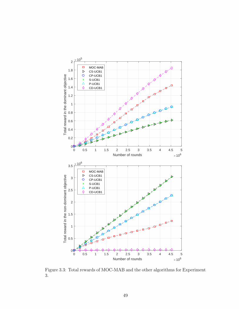
0 0.5 1 1.5 2 2.5 3 3.5 4 4.5 5

Number of rounds 106

0

0.2

0.4

0.6

0.8

1

1.2

1.4

1.6

1.8

2T

otal

rew

ard

in th

e do

min

ant o

bjec

tive

105

MOC-MABCS-UCB1CP-UCB1S-UCB1P-UCB1CD-UCB1

0 0.5 1 1.5 2 2.5 3 3.5 4 4.5 5

Number of rounds 106

0

0.5

1

1.5

2

2.5

3

3.5

Tot

al r

ewar

d in

the

non-

dom

inan

t obj

ectiv

e

106

MOC-MABCS-UCB1CP-UCB1S-UCB1P-UCB1CD-UCB1

Figure 3.3: Total rewards of MOC-MAB and the other algorithms for Experiment3.

49

Chapter 4

Multi-objective Contextual

X -armed Bandit

In this chapter, we consider a multi-objective contextual MAB problem with

an arbitrary number of objectives and a high-dimensional, possibly uncountable

arm set (also called multi-objective contextual X -armed bandit problem). First

section includes problem formulation and the definition of the contextual Pareto

regret (referred to as the Pareto regret hereafter), which is defined in [19] for two

objectives. Here, we extend it to work for an arbitrary number of objectives. For

this problem, we propose an online learning algorithm called Pareto Contextual

Zooming (PCZ) in Section 4.2 and its Pareto regret is analyzed in Section 4.3.

We prove that the regret bound of PCZ is nearly optimal by providing an almost

matching lower bound in Section 4.4. Lastly, we evaluate the performance of PCZ

in synthetic dataset in Section 4.5. This work was published in [12].1

1E. Turgay, D. Oner, and C. Tekin, ”Multi-objective contextual bandit problem with sim-ilarity information” in Proc. 21st. Int. Conf. on Artificial Intelligence and Statistics, pp.1673-1681, 2018.

50

4.1 Problem Formulation

The system operates in rounds indexed by t ∈ 1, 2, . . .. At the beginning of

each round, the learner observes a context xt that comes from a dx-dimensional

context set X . Then, the learner chooses an arm at from a da-dimensional arm set

A. After choosing the arm, the learner obtains a dr-dimensional random reward

vector rt := (r1t , . . . , rdrt ) where rit denotes the reward obtained from objective

i ∈ 1, . . . , dr in round t. Let µia(x) denote the expected reward of arm a in

objective i for context x and µa(x) := (µ1a(x), . . . , µdra (x)). The random reward

vector obtained from arm at in round t is given as rt := µat(xt) + κt where κt is

the dr-dimensional noise process whose marginal distribution for each objective

is conditionally 1-sub-Gaussian, i.e., ∀λ ∈ R

E[eλκit | a1:t, x1:t, κ1:t−1] ≤ exp (λ2/2)

where b1:t := (b1, . . . , bt). Context and arm sets together constitute the set of

feasible context-arm pairs, denoted by F := X × A. We assume that the Lips-

chitz condition holds for the set of feasible context-arm pairs with respect to the

expected rewards for all objectives.

Assumption 3. For all i ∈ 1, . . . , dr, a, a′ ∈ A and x, x′ ∈ X , we have

|µia(x)− µia′(x′)| ≤ D((x, a), (x′, a′))

where D is the distance function known by the learner such that D((x, a), (x′, a′)) ≤1 for all x, x′ ∈ X and a, a′ ∈ A.

(F , D) denotes the similarity space. In the multi-objective bandit problem,

since the objectives might be conflicting, finding an arm that simultaneously

maximizes the expected reward in all objectives is in general not possible. Thus,

an intuitive way to define optimality is to use the notion of Pareto optimality.

Definition 3 (Pareto optimality). (i) An arm a is weakly dominated by arm

a′ given context x, denoted by µa(x) µa′(x) or µa′(x) µa(x), if µia(x) ≤µia′(x),∀i ∈ 1, . . . , dr.

51

(ii) An arm a is dominated by arm a′ given context x, denoted by µa(x) ≺ µa′(x)

or µa′(x) µa(x), if it is weakly dominated and ∃i ∈ 1, . . . , dr such that

µia(x) < µia′(x).

(iii) Two arms a and a′ are incomparable given context x, denoted by

µa(x)||µa′(x), if neither arm dominates the other.

(iv) An arm is Pareto optimal given context x if it is not dominated by any other

arm given context x. The set of all Pareto optimal arms given a particular context

x, is called the Pareto front, and is denoted by O(x).

The expected loss incurred by the learner in a round due to not choosing an

arm in the Pareto front is equal to the Pareto suboptimality gap (PSG) of the

chosen arm, which is defined as follows.

Definition 4 (PSG). The PSG of an arm a ∈ A given context x, denoted by

∆a(x), is defined as the minimum scalar ε ≥ 0 that needs to be added to all

entries of µa(x) such that a becomes a member of the Pareto front. Formally,

∆a(x) := infε≥0

ε s.t. (µa(x) + ε) || µa′(x),∀a′ ∈ O(x)

where ε is a dr-dimensional vector, whose entries are ε.

We evaluate the performance of the learner using the Pareto regret, which is

given as

PR(T ) :=T∑t=1

∆at(xt). (4.1)

The Pareto regret measures the total loss due to playing arms that are not in

the Pareto front. The goal of the learner is to minimize its Pareto regret while

ensuring fairness over the Pareto optimal arms for the observed contexts. Our

regret bounds depend on the Pareto zooming dimension, which is defined below.

Definition 5. (i) F ⊂ F is called an r-packing of F if all z, z′ ∈ F satis-

fies D(z, z′) ≥ r. For any r > 0, the r-packing number of F is Apackingr (F) :=

max|F | : F is an r-packing of F.(ii) For a given r > 0, let Fµ,r := (x, a) ∈ F : ∆a(x) ≤ 12r denote the set of

52

near-optimal context-arm pairs. The Pareto r-zooming number Nr is defined as

the r-packing number of Fµ,r.(iii) The Pareto zooming dimension given any constant c > 0 is defined as

dp(c) := infd > 0 : Nr ≤ cr−d,∀r ∈ (0, 1). With an abuse of notation we

let dp := dp(p) for p > 0.

4.2 Pareto Contextual Zooming Algorithm

(PCZ)

In this section, we present a multi-objective contextual bandit algorithm called

Pareto Contextual Zooming (PCZ). Pseudo-code of PCZ is given in Algorithm

2. PCZ is a multi-objective extension of the single objective contextual zoom-

ing algorithm [7]. The proposed algorithm partitions the similarity space non-

uniformly according to the arms selected, and the contexts and rewards observed

in the past by using a set of active balls B which may change from round to

round. Each active ball B ∈ B has a radius r(B), center (xB, aB) and a domain

in the similarity space. The domain of ball B at the beginning of round t is

denoted by domt(B), and is defined as the subset of B that excludes all active

balls at the beginning of round t that have radius strictly smaller than r(B), i.e.,

domt(B) := B \ (∪B′∈B:r(B′)<r(B)B′). The domains of all active balls cover the

similarity space.

Initially, PCZ takes as inputs the time horizon T ,2 the similarity space (F , D),

the confidence parameter δ ∈ (0, 1), and creates an active ball centered at a

random point in the similarity space with radius 1 whose domain covers the entire

similarity space. At the beginning of round t, PCZ observes the context xt, and

finds the set of relevant balls denoted by R(xt) := B ∈ B : (xt, a) ∈ domt(B)

for some a ∈ A.

After finding the set of relevant balls, PCZ uses the principle of optimism under

2While PCZ requires T as input, it is straightforward to extend it to work without knowingT beforehand, by using a standard method, called the doubling trick.

53

the face of uncertainty to select a ball and an arm. In this principle, the estimated

rewards of the balls are inflated by a certain level, such that the inflated reward

estimates (also called indices) become an upper confidence bound (UCB) for the

expected reward with high probability. Then, PCZ selects a ball whose index is

in the Pareto front. In general, this allows the balls that are rarely selected to get

explored (because their indices will remain high due to the sample uncertainty

being high), which enables the learner to discover new balls that are potentially

better than the frequently selected balls in terms of the rewards.

Algorithm 2 Pareto Contextual Zooming

1: Input: (F , D), T , δ2: Data: Collection B of ”active balls” in (F ,D); counters NB and estimatesµiB, ∀B ∈ B, ∀i ∈ 1, . . . , dr

3: Init: Create ball B, with r(B) = 1 and an arbitrary center in F . B ← B4: µiB = 0, ∀i ∈ 1, . . . , dr and NB = 05: while 1 ≤ t ≤ T do6: Observe xt7: R(xt)← B ∈ B : (xt, a) ∈ domt(B) for some a ∈ A8: B∗ ← B ∈ R(xt) : gB 6≺ gB′ , ∀B′ ∈ R(xt)9: Select an arm at uniformly at random from a : (xt, a) ∈ ∪B∈B∗domt(B),

and observe the rewards ri, ∀i ∈ 1, . . . , dr10: Uniformly at random choose a ball B ∈ B∗ whose domain contains (xt, at)11: if uB ≤ r(B) then12: Activate (create) a new ball B′ whose center is (xt, at) and radius is

r(B′) = r(B)/213: B ← B ∪B′, and µiB′ = NB′ = 0, ∀i ∈ 1, . . . , dr.14: Update the domains of balls in B.15: end if16: Update estimates µi

B= ((µi

BNB) + ri)/(NB + 1), ∀i ∈ 1, . . . , dr and the

counter NB = NB + 117: end while

The index for each relevant ball is calculated in the following way: First, PCZ

computes a pre-index for each ball in B given by

gi,preB :=µiB + uB + r(B), i ∈ 1, . . . , dr

which is the sum of the sample mean reward µiB, the sample uncertainty uB :=√2AB/NB, where AB := (1 + 2 log(2

√2drT

32/δ)) and NB is the number of times

ball B is chosen, and the contextual uncertainty r(B). The sample uncertainty

54

represents the uncertainty in the sample mean estimate of the expected reward

due to the limited number of random samples in ball B that are used to form

this estimate. On the other hand, the contextual uncertainty represents the

uncertainty in the sample mean reward due to the dissimilarity of the contexts

that lie within ball B. When a ball is selected, its sample uncertainty decreases

but its contextual uncertainty is always fixed. Essentially, the pre-index gi,preB is

a UCB for the expected reward at the center of ball B in objective i. PCZ uses

these pre-indices to compute an index for each relevant ball, given as

gB := (g1B, . . . , gdrB ) where

giB :=r(B) + minB′∈B

(gi,preB′ +D(B′, B))

and D(B′, B) represents the distance between the centers of the balls B′ and B

in the similarity space.

After the indices of the relevant balls are calculated, PCZ computes the Pareto

front among the set of balls in R(xt) by using gB for ball B ∈ R(xt) as a proxy

for the expected reward (see Definition 3), which is given as B∗ := B ∈ R(xt) :

gB 6≺ gB′ ,∀B′ ∈ R(xt), and uniformly at random selects an arm in the union of

the domains of the balls whose indices are in the Pareto front. After observing

the reward of the selected arm, it uniformly at random picks a ball whose index

is in the Pareto front and contains (xt, at), updates its parameters, and the above

procedure repeats in the next round. This selection ensures fairness over the

estimated set of Pareto optimal arms in each round.

The remaining important issue is how to create the balls in order to trade-

off sample uncertainty and contextual uncertainty in an optimal way. This is a

difficult problem due to the fact that the learner does not know how contexts

arrive beforehand, and the rate that the contexts arrive in different regions of the

context set can dynamically change over time. To overcome these issues, PCZ

uses the concept of contextual zooming. Basically, PCZ adaptively partitions the

context space according to the past context arrivals, arm selections and obtained

rewards. Specifically, the radius of the balls are adjusted to optimize the two

sources of error described above. For this, when the sample uncertainty of the

selected ball B is found to be smaller than or equal to the radius of the ball (say

55

in round t), a new child ball B′ centered at (xt, at) whose radius is equal to the

half of the parent ball’s (ball B’s) radius is created, and the domains of all active

balls are updated.3 Note that when a child ball is created, it does not contain any

sample, so its sample uncertainty is infinite. This results in an infinite pre-index.

For this reason, giB is used instead of gi,preB as an enhanced UCB, which is in

general tighter than the UCB based on the pre-index.

4.3 Regret Analysis of PCZ

In this section, we prove that PCZ achieves (i) O(T (1+dp)/(2+dp)) Pareto regret

with probability at least 1− δ, and (ii) O(T (1+dp)/(2+dp)) expected Pareto regret,

where dp is the Pareto zooming dimension.

First, we define the variables that will be used in the Pareto regret analysis.

For an event H, let Hc denote the complement of that event. For all the parame-

ters defined in the pseudo-code of PCZ, we explicitly use the round index t, when

referring to the value of that parameter at the beginning of round t. For instance,

NB(t) denotes the value of NB at the beginning of round t, and B(t) denotes the

set of balls created by PCZ by the beginning of round t. Let B′(T ) denote the set

of balls chosen at least once by the end of round T . Note that B′(T ) ⊂ B(T ) and

B(T ) is a random variable that depends both on the contexts arrivals, selected

arms and observed rewards. Let RiB(t) denote the random reward of ball B in

objective i at round t and let τB(t) denote the first round after the round in which

ball B is chosen by PCZ for the tth time. Moreover, the round that comes just

after B ∈ B(T ) is created is denoted by τB(0), and the domain of B when it is

created is denoted by dom(B). Hence, domt(B) ⊆ dom(B), ∀t ∈ τB(0), . . . , T.For B ∈ B′(T ), let TB denote the set of rounds in τB(0), . . . , T in which ball

B is selected by PCZ. Also let xB(t) := xτB(t)−1, aB(t) := aτB(t)−1, RiB(t) :=

RiB(τB(t) − 1), κiB(t) := κiτB(t)−1, NB(t) := NB(τB(t)), µiB(t) := µiB(τB(t)),

gi,preB (t) := gi,preB (τB(t)), giB(t) := giB(τB(t)), and uB(t) := uB(τB(t)). We note

3We also use Bpar to denote the parent of a ball B.

56

that all inequalities that involve random variables hold with probability one un-

less otherwise stated. Let

PRB(T ) :=

NB(T+1)∑t=1

∆aB(t)(xB(t))

denote the Pareto regret incurred in ball B ∈ B′(T ) for rounds in TB. Then, the

Pareto regret in (4.1) can be written as

PR(T ) =∑

B∈B′(T )

PRB(T ).

Next, we define the following lower and upper bounds: LiB(t) := µiB(t) − uB(t)

and U iB(t) := µiB(t) + uB(t), LiB(t) := µiB(t)− uB(t) and U i

B(t) := µiB(t) + uB(t)

for i ∈ 1, . . . , dr. Let

UCiB :=

T+1⋃t=τB(0)

µiaB(xB) /∈ [LiB(t)− r(B), U iB(t) + r(B)]

denote the event that the learner is not confident about its reward estimate in

objective i in ball B for at least once from round τB(0) to round T , and

UCi

B :=

NB(T+1)⋃t=0

µiaB(xB) /∈ [LiB(t)− r(B), U iB(t) + r(B)].

Let τB(NB(T + 1) + 1) = T + 2. Then, for z = 0, . . . , NB(T + 1) the events

µiaB(xB) /∈ [LiB(t)−r(B), U iB(t)+r(B)] and µiaB(xB) /∈ [LiB(t′)−r(B), U i

B(t′)+

r(B)] are identical for any t, t′ ∈ τB(z), . . . , τB(z + 1)− 1. Thus,

τB(z+1)−1⋃t=τB(z)

µiaB(xB) /∈ [LiB(t)− r(B), U iB(t) + r(B)]

= µiaB(xB) /∈ [LiB(z)− r(B), U iB(z) + r(B)].

Hence, we conclude that UCiB = UC

i

B. Let UCB := ∪i∈1,...,drUCiB and UC :=

∪B∈B(T )UCB. Next, we will bound E[PR(T )]. We have

E[PR(T )] = E[PR(T ) | UC] Pr(UC) + E[PR(T ) | UCc] Pr(UCc)

≤ CmaxT Pr(UC) + E[PR(T ) | UCc] (4.2)

57

where Cmax := sup(x,a)∈F ∆a(x). Since B(T ) is a random variable, we have

Pr(UC) =

∫Pr(UC|B(T ))dQ(B(T )) (4.3)

where Q(B(T )) denotes the distribution of B(T ). We also have

Pr(UC|B(T )) = Pr(∪B∈B(T )UCB|B(T )) ≤∑

B∈B(T )

Pr(UCB|B(T )). (4.4)

We proceed by bounding the term Pr(UC) in (4.2). For this, first we bound

Pr(UCB|B(T )) in the next lemma.

Lemma 7. When PCZ is run, we have Pr(UCB|B(T )) ≤ δ/T , ∀B ∈ B(T ).

Proof. From the definitions of LiB(t), U iB(t) and UC

i

B, it can be observed that

the event UCiB happens when µiB(t) remains away from µiaB(xB) for some

t ∈ 0, . . . , NB(T + 1). Using this information, we can use the concentration

inequality given in Appendix B. In this formulation expected rewards of the

arms must be equal in all rounds, but in our case, µiaB(t)(xB(t)) changes since the

elements of xB(t), aB(t)NB(T+1)t=1 are not identical which makes distributions of

RiB(t), t ∈ 1, . . . , NB(T + 1) different.

In order to overcome this issue, we use the sandwich technique proposed in [6]

and later used in [19]. For any ball B ∈ B(T ), we have Pr(µiaB(xB) /∈ [LiB(0) −r(B), U i

B(0) + r(B)]) = 0 since µiB(0) = 0, LiB(0) = −∞ and U iB(0) = ∞.

Thus, for B ∈ B(T ) \ B′(T ), we have Pr(UCB|B(T )) = 0. Hence, we proceed by

bounding the probabilities of the events µiaB(xB) /∈ [LiB(t)−r(B), U iB(t)+r(B)],

for t > 0 and for the balls in B′(T ). Recall that RiB(t) = µiaB(t)(xB(t)) + κiB(t)

and µiB(t) =∑t

l=1 RiB(l)/t (for t > 0 and B ∈ B′(T )). For each i ∈ 1, . . . , dr,

B ∈ B′(T ), let

µiB = sup(x,a)∈dom(B)

µia(x) and µiB

= inf(x,a)∈dom(B)

µia(x).

We define two new sequences of random variables, whose sample mean val-

ues will lower and upper bound µiB(t). The best sequence is defined as

RiB(t)NB(T+1)

t=1 where Ri

B(t) := µiB + κiB(t), and the worst sequence is defined

58

as RiB(t)NB(T+1)

t=1 where RiB(t) := µi

B+ κiB(t). Let µiB(t) :=

∑tl=1R

i

B(l)/t and

µiB

(t) :=∑t

l=1RiB(l)/t. We have

µiB

(t) ≤ µiB(t) ≤ µiB(t) ∀t ∈ 1, . . . , NB(T + 1).

Let

Li

B(t) := µiB(t)− uB(t)

Ui

B(t) := µiB(t) + uB(t)

LiB(t) := µiB

(t)− uB(t)

U iB(t) := µi

B(t) + uB(t).

It can be shown that

µiaB(xB) /∈ [LiB(t)− r(B), U iB(t) + r(B)] (4.5)

⊂ µiaB(xB) /∈ [Li

B(t)− r(B), Ui

B(t) + r(B)]

∪ µiaB(xB) /∈ [LiB(t)− r(B), U iB(t) + r(B)].

Moreover, the following inequalities can be obtained from Assumption 3:

µiaB(xB) ≤ µiB ≤ µiaB(xB) + r(B) (4.6)

µiaB(xB)− r(B) ≤ µiB≤ µiaB(xB). (4.7)

Using (4.6) and (4.7) it can be shown that

µiaB(xB) /∈ [Li

B(t)− r(B), Ui

B(t) + r(B)] ⊂ µiB /∈ [Li

B(t), Ui

B(t)],

µiaB(xB) /∈ [LiB(t)− r(B), U iB(t) + r(B)] ⊂ µi

B/∈ [LiB(t), U i

B(t)].

Plugging this to (4.5), we get

µiaB(xB) /∈ [LiB(t)− r(B), U iB(t) + r(B)]

⊂ µiB /∈ [Li

B(t), Ui

B(t)]⋃µi

B/∈ [LiB(t), U i

B(t)].

Using the equation above and the union bound we obtain

Pr(UCiB|B(T )) ≤ Pr

NB(T+1)⋃t=1

µiB /∈ [Li

B(t), Ui

B(t)]

59

+ Pr

NB(T+1)⋃t=1

µiB/∈ [LiB(t), U i

B(t)]

.

Both terms on the right-hand side of the inequality above can be bounded using

the concentration inequality in Appendix B. Using θ = δ/(2drT ), in Appendix B

gives Pr(UCiB|B(T )) ≤ δ/(drT ), since 1 + NB(t) ≤ 1 + NB(T + 1) ≤ 2T . Then,

using the union bound over all objectives, we obtain Pr(UCB|B(T )) ≤ δ/T .

Next, we bound Pr(UC). Since |B(T )| ≤ T , by using union bound over all

created balls, (4.3) and (4.4) we obtain

Pr(UC) ≤∫

Pr(UC|B(T ))dQ(B(T ))

≤∫ ( ∑

B∈B(T )

Pr(UCB|B(T ))

)dQ(B(T ))

≤ δT

T

∫dQ(B(T )) ≤ δ.

Then, by using (4.2),

E[PR(T )] ≤ CmaxT Pr(UC) + E[PR(T ) | UCc] ≤ CmaxTδ + E[PR(T ) | UCc].

(4.8)

In the remainder of the analysis we bound PR(T ) on event UCc. Then, we

conclude the analysis by using this to bound 4.8. For simplicity of notation, in

the following lemmas we use B(t) to denote the ball selected in round t.

Lemma 8. Consider a virtual arm with expected reward vector gB(t)(t), where

giB(t)(t) denotes the expected reward in objective i. On event UCc, we have

gB(t)(t) 6≺ µa(xt),∀a ∈ A.

Proof. For any relevant ball B ∈ R(xt) and i ∈ 1, . . . , dr, let Bi :=

arg minB′∈B(t)gi,preB′ (t) + D(B,B′). Then, ∀a such that (xt, a) ∈ domt(B), we

have

giB(t) = r(B) + gi,preBi

(t) +D(B, Bi)

60

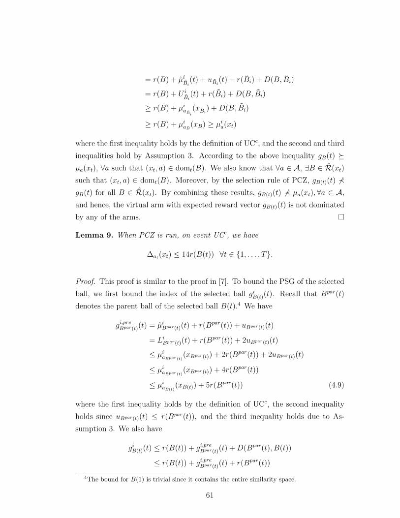
= r(B) + µiBi

(t) + uBi(t) + r(Bi) +D(B, Bi)

= r(B) + U iBi

(t) + r(Bi) +D(B, Bi)

≥ r(B) + µiaBi(xBi) +D(B, Bi)

≥ r(B) + µiaB(xB) ≥ µia(xt)

where the first inequality holds by the definition of UCc, and the second and third

inequalities hold by Assumption 3. According to the above inequality gB(t) µa(xt), ∀a such that (xt, a) ∈ domt(B). We also know that ∀a ∈ A, ∃B ∈ R(xt)

such that (xt, a) ∈ domt(B). Moreover, by the selection rule of PCZ, gB(t)(t) 6≺gB(t) for all B ∈ R(xt). By combining these results, gB(t)(t) 6≺ µa(xt),∀a ∈ A,

and hence, the virtual arm with expected reward vector gB(t)(t) is not dominated

by any of the arms.

Lemma 9. When PCZ is run, on event UCc, we have

∆at(xt) ≤ 14r(B(t)) ∀t ∈ 1, . . . , T.

Proof. This proof is similar to the proof in [7]. To bound the PSG of the selected

ball, we first bound the index of the selected ball giB(t)(t). Recall that Bpar(t)

denotes the parent ball of the selected ball B(t).4 We have

gi,preBpar(t)(t) = µiBpar(t)(t) + r(Bpar(t)) + uBpar(t)(t)

= LiBpar(t)(t) + r(Bpar(t)) + 2uBpar(t)(t)

≤ µiaBpar(t)(xBpar(t)) + 2r(Bpar(t)) + 2uBpar(t)(t)

≤ µiaBpar(t)(xBpar(t)) + 4r(Bpar(t))

≤ µiaB(t)(xB(t)) + 5r(Bpar(t)) (4.9)

where the first inequality holds by the definition of UCc, the second inequality

holds since uBpar(t)(t) ≤ r(Bpar(t)), and the third inequality holds due to As-

sumption 3. We also have

giB(t)(t) ≤ r(B(t)) + gi,preBpar(t)(t) +D(Bpar(t), B(t))

≤ r(B(t)) + gi,preBpar(t)(t) + r(Bpar(t))

4The bound for B(1) is trivial since it contains the entire similarity space.

61

≤ r(B(t)) + µiaB(t)(xB(t)) + 6r(Bpar(t))

≤ µiaB(t)(xB(t)) + 13r(B(t))

≤ µiat(xt) + 14r(B(t))

where the third inequality follows from (4.9). Since giB(t)(t)−µiat(xt) ≤ 14r(B(t))

for all i ∈ 1, . . . , dr and the virtual arm is not dominated by any arm in the

Pareto front by Lemma 8, the PSG of the selected arm is bounded by ∆at(xt) ≤14r(B(t)).

Lemma 10. When PCZ is run, on event UCc, the maximum number of radius

r balls that are created by round T is bounded by the Pareto r-zooming number

Nr given in Definition 5. Moreover, in any round t in which a radius r ball is

created, we have ∆at(xt) ≤ 12r.

Proof. Assume that a new ball is created at round t whose parent is B(t). Let

B′(t) denote the created ball. We have,

giB(t)(t) ≤ r(B(t)) + gi,preB(t) (t)

= µiB(t)(t) + 2r(B(t)) + uB(t)(t)

= LiB(t)(t) + 2r(B(t)) + 2uB(t)(t)

≤ µiaB(t)(xB(t)) + 3r(B(t)) + 2uB(t)(t)

≤ µiaB(t)(xB(t)) + 5r(B(t))

≤ µiaB′(t)(xB′(t)) + 6r(B(t))

≤ µiaB′(t)(xB′(t)) + 12r(B′(t))

where the first inequality follows from the definition of giB(t)(t), the second in-

equality holds by the definition of UCc, the third inequality holds due to the fact

that B(t) is a parent ball, the fourth inequality holds due to Assumption 3, and

the last inequality follows from r(B′(t)) = r(B(t))/2. Similar to the proof of

Lemma 9, since giB(t)(t) − µiaB′(t)(xB′(t)) ≤ 12r(B′(t)) for all i ∈ 1, . . . , dr and

the virtual arm is not dominated by any arm in the Pareto front by Lemma 8, the

PSG of point (xB′(t), aB′(t)) = (xt, at) is bounded by 12r(B′(t)). This implies that

center of the ball created in any round t has a PSG that is at most 12r(B′(t)).

62

Thus, the center of B′(t) is in Fµ,r(B′(t)). Next, consider any two balls B and B′

with radius r created by PCZ. Based on the ball creation and domain update

rules of PCZ, the distance between the centers of these balls must be at least r.

As a result, the maximum number of radius r balls created is bounded by the

r-packing number of Fµ,r, which is Nr.

The following lemma bounds the regret of PCZ in terms of Nr by using the

results in Lemma 10 and 9.

Lemma 11. On event UCc, the Pareto regret of PCZ by round T is bounded by

PR(T ) ≤ 28Tr0 +∑

r=2−i:i∈N,r0≤r≤1 56r−1Nr log(2√

2drT32 e/δ) for any r0 ∈ (0, 1].

Proof. The maximum number of times a radius r ball B can be selected before

it becomes a parent ball is upper bounded by 1 + 2r−2(1 + 2 log(2√

2drT32/δ)).

From the result of Lemma 9, we know that the Pareto regret in each of these

rounds is upper bounded by 14r. Note that after ball B becomes a parent ball,

it will create a new radius r/2 child ball every time it is selected. From Lemma

10, we know that the Pareto regret in each of these rounds is bounded above by

12(r/2). Therefore, we can include the Pareto regret incurred in a round in which

a new child ball with radius r is created from a parent ball as a part of the child

ball’s (total) Pareto regret. Hence, the Pareto regret incurred in a radius r ball

is upper bounded by

14r(

1 + 2r−2(1 + 2 log(2√

2drT32/δ))

)+ 12r

≤ 14r(

2 + 2r−2(1 + 2 log(2√

2drT32/δ))

)≤ 56r−1 log(2

√2drT

32 e/δ).

Let rl := 2dlog(r0)/ log(2)e. We have r0/2 ≤ rl/2 ≤ r0 ≤ rl ≤ 2r0. The one-round

Pareto regret of the balls whose radii are smaller than rl is bounded by 14rl on

event UCc according to Lemma 9. Also, we know that 14rl ≤ 28r0 by the above

inequality. Therefore, the Pareto regret due to all balls with radii smaller than rl

by time T is bounded by 28Tr0, and the Pareto regret due to all balls with radii

63

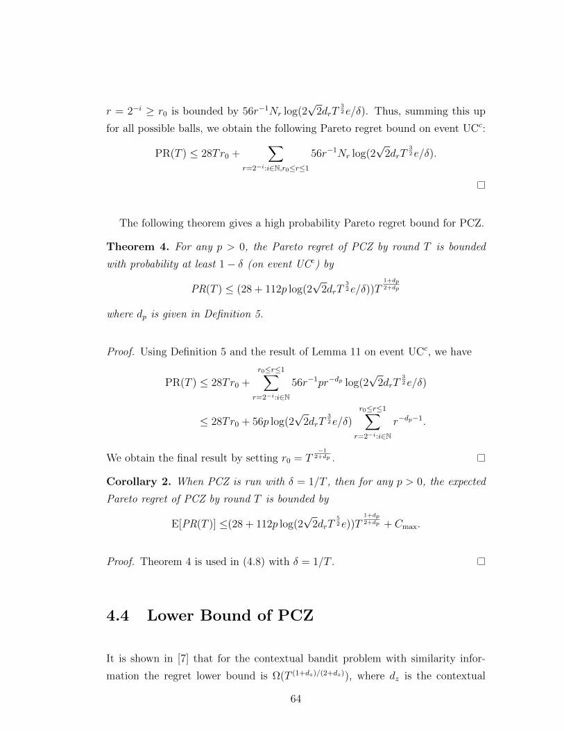
r = 2−i ≥ r0 is bounded by 56r−1Nr log(2√

2drT32 e/δ). Thus, summing this up

for all possible balls, we obtain the following Pareto regret bound on event UCc:

PR(T ) ≤ 28Tr0 +∑

r=2−i:i∈N,r0≤r≤1

56r−1Nr log(2√

2drT32 e/δ).

The following theorem gives a high probability Pareto regret bound for PCZ.

Theorem 4. For any p > 0, the Pareto regret of PCZ by round T is bounded

with probability at least 1− δ (on event UCc) by

PR(T ) ≤ (28 + 112p log(2√

2drT32 e/δ))T

1+dp2+dp

where dp is given in Definition 5.

Proof. Using Definition 5 and the result of Lemma 11 on event UCc, we have

PR(T ) ≤ 28Tr0 +

r0≤r≤1∑r=2−i:i∈N

56r−1pr−dp log(2√

2drT32 e/δ)

≤ 28Tr0 + 56p log(2√

2drT32 e/δ)

r0≤r≤1∑r=2−i:i∈N

r−dp−1.

We obtain the final result by setting r0 = T−1

2+dp .

Corollary 2. When PCZ is run with δ = 1/T , then for any p > 0, the expected

Pareto regret of PCZ by round T is bounded by

E[PR(T )] ≤(28 + 112p log(2√

2drT52 e))T

1+dp2+dp + Cmax.

Proof. Theorem 4 is used in (4.8) with δ = 1/T .

4.4 Lower Bound of PCZ

It is shown in [7] that for the contextual bandit problem with similarity infor-

mation the regret lower bound is Ω(T (1+dz)/(2+dz)), where dz is the contextual

64

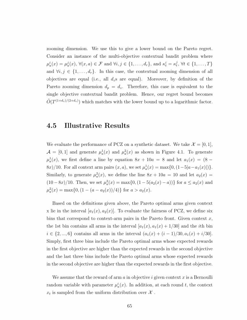
zooming dimension. We use this to give a lower bound on the Pareto regret.

Consider an instance of the multi-objective contextual bandit problem where

µia(x) = µja(x), ∀(x, a) ∈ F and ∀i, j ∈ 1, . . . , dr, and κit = κjt , ∀t ∈ 1, . . . , Tand ∀i, j ∈ 1, . . . , dr. In this case, the contextual zooming dimension of all

objectives are equal (i.e., all dzs are equal). Moreover, by definition of the

Pareto zooming dimension dp = dz. Therefore, this case is equivalent to the

single objective contextual bandit problem. Hence, our regret bound becomes

O(T (1+dz)/(2+dz)) which matches with the lower bound up to a logarithmic factor.

4.5 Illustrative Results

We evaluate the performance of PCZ on a synthetic dataset. We take X = [0, 1],

A = [0, 1] and generate µ1a(x) and µ2

a(x) as shown in Figure 4.1. To generate

µ1a(x), we first define a line by equation 8x + 10a = 8 and let a1(x) = (8 −

8x)/10. For all context arm pairs (x, a), we set µ1a(x) = max0, (1−5|a−a1(x)|).

Similarly, to generate µ2a(x), we define the line 8x + 10a = 10 and let a2(x) =

(10− 8x)/10. Then, we set µ2a(x) = max0, (1− 5(a2(x)− a)) for a ≤ a2(x) and

µ2a(x) = max0, (1− (a− a2(x))/4) for a > a2(x).

Based on the definitions given above, the Pareto optimal arms given context

x lie in the interval [a1(x), a2(x)]. To evaluate the fairness of PCZ, we define six

bins that correspond to context-arm pairs in the Pareto front. Given context x,

the 1st bin contains all arms in the interval [a1(x), a1(x) + 1/30] and the ith bin

i ∈ 2, ..., 6 contains all arms in the interval (a1(x) + (i − 1)/30, a1(x) + i/30].

Simply, first three bins include the Pareto optimal arms whose expected rewards

in the first objective are higher than the expected rewards in the second objective

and the last three bins include the Pareto optimal arms whose expected rewards

in the second objective are higher than the expected rewards in the first objective.

We assume that the reward of arm a in objective i given context x is a Bernoulli

random variable with parameter µia(x). In addition, at each round t, the context

xt is sampled from the uniform distribution over X .

65

0 0.1 0.2 0.3 0.4 0.5 0.6 0.7 0.8 0.9 1

Context x

0

0.1

0.2

0.3

0.4

0.5

0.6

0.7

0.8

0.9

1

Arm

a

1a(x)

0 0.1 0.2 0.3 0.4 0.5 0.6 0.7 0.8 0.9 1

Context x

0

0.1

0.2

0.3

0.4

0.5

0.6

0.7

0.8

0.9

1

Arm

a

2a(x)

Figure 4.1: Expected reward of Context-Arm Pairs (Yellow represents 1, DarkBlue represents 0)

We compare our algorithm with Contextual Zooming [7] and Random Selec-

tion, which chooses in each round an arm uniformly at random from A. Con-

textual Zooming only uses the rewards in the first objective. Both PCZ and

Contextual Zooming uses scaled Euclidean distance.5 We choose δ = 1/T in

PCZ, set T = 105, run each algorithm 100 times, and report the average of the

results in these runs.

The Pareto Regret is reported in Figure 4.2(i) as a function of the number

5We set D((x, a), (x′, a′)) =√

(x− x′)2 + (a− a′)2/√

2. While this choice does not satisfyAssumption 3, we use this setup to illustrate that learning is still possible when the distancefunction is not perfectly known by the learner.

66

of rounds. It is observed that the Pareto regret of PCZ at T = 105 is 3.61%

higher than that of Contextual Zooming and 17.1% smaller than that of Random

Selection. We compare the fairness of the algorithms in Figure 4.2(ii). For this,

we report the selection ratio of each Pareto front bin, which is defined for bin

i as the number of times a context-arm pair in bin i is selected divided by the

number of times a Pareto optimal arm is selected by round T . We observe that

the selection ratio of all bins are almost the same for PCZ, while Contextual

Zooming selects the context-arm pairs in the 1st bin much more than the other

bins.

67

0 1 2 3 4 5 6 7 8 9 10

Number of Rounds 104

0

2000

4000

6000

8000

10000

12000

14000

16000

18000P

aret

o R

egre

t

Pareto Contextual ZoomingContextual ZoomingRandom Selection

1 2 3 4 5 6

Pareto Front Bins

0

0.05

0.1

0.15

0.2

0.25

Sel

ectio

n R

atio

s of

the

Par

eto

Fro

nt B

ins

Pareto Contextual ZoomingContextual ZoomingRandom Selection

Figure 4.2: (i) Pareto Regret vs. Number of Rounds (ii) Selection Ratio of thePareto Front Bins

68

Chapter 5

Conclusion and Future Works

In this thesis, we consider two different multi-objective contextual MAB prob-

lems. In the first one, we propose a novel contextual MAB problem with two

objectives in which one objective is dominant and the other is non-dominant. We

also propose a new performance metric called 2D regret which is a vector whose

ith component corresponds to the difference between the expected total reward

of an oracle in objective i that selects optimal arm for each context and that of

the learner by round T . We extend the Pareto regret proposed in [10] to take into

account the dependence of the Pareto front on the context. For this problem, we

propose a multi-objective contextual multi-armed bandit algorithm (MOC-MAB)

and we prove that both the 2D regret and the Pareto regret of MOC-MAB are

sublinear in the number of rounds. However, MOC-MAB partitions the context

space uniformly and it is not an optimal solution when context sampling distri-

bution is complex. For the future, we will work on this problem by considering

adaptive partition and by this way, our initial assumption is to provide tighter

regret bounds in the 2D and the Pareto regret. In the second work of the thesis,

we consider a multi-objective contextual MAB problem with an arbitrary number

of objectives and a high-dimensional, possibly uncountable arm set. Then, we

propose an online learning algorithm called Pareto Contextual Zooming (PCZ)

and prove that Pareto regret of PCZ is sublinear in the number of rounds. We

69

also show an almost matching lower bound Ω(T (1+dp)/(2+dp)) based on a reduc-

tion to the classical contextual bandit problem with similarity information, which

shows that our bound is tight up to logarithmic factors. Performance of PCZ is

demonstrated in the simulations and we show that PCZ randomly alternates be-

tween the arms in the estimated Pareto front and ensures the arms in this set are

fairly selected. Future work will focus on evaluating the Pareto regret and the

fairness of the proposed algorithm in real-world datasets.

70

Bibliography

[1] Y. Abbasi-Yadkori, D. Pal, and C. Szepesvari, “Improved algorithms for lin-

ear stochastic bandits,” in Proc. 25th Conf. in Neural Information Processing

Systems, pp. 2312–2320, 2011.

[2] D. Russo and B. Van Roy, “Learning to optimize via posterior sampling,”

Mathematics of Operations Research, vol. 39, no. 4, pp. 1221–1243, 2014.

[3] H. Robbins, “Some aspects of the sequential design of experiments,” in Her-

bert Robbins Sel. Papers, pp. 169–177, Springer, 1985.

[4] Y. Gai, B. Krishnamachari, and R. Jain, “Learning multiuser channel al-

locations in cognitive radio networks: A combinatorial multi-armed bandit

formulation,” in Proc. 4th IEEE Symposium on New Frontiers in Dynamic

Spectrum, pp. 1–9, 2010.

[5] L. Li, W. Chu, J. Langford, and R. E. Schapire, “A contextual-bandit ap-

proach to personalized news article recommendation,” in Proc. 19th Int.

Conf. on World Wide Web, pp. 661–670, 2010.

[6] C. Tekin, J. Yoon, and M. van der Schaar, “Adaptive ensemble learning with

confidence bounds,” IEEE Transactions on Signal Processing, vol. 65, no. 4,

pp. 888–903, 2017.

[7] A. Slivkins, “Contextual bandits with similarity information,” J. of Machine

Learning Research, vol. 15, no. 1, pp. 2533–2568, 2014.

[8] T. Lu, D. Pal, and M. Pal, “Contextual multi-armed bandits,” in Proc. 13th

Int. Conf. on Artificial Intelligence and Statistics, pp. 485–492, 2010.

71

[9] M. Rodriguez, C. Posse, and E. Zhang, “Multiple objective optimization in

recommender systems,” in Proc. 6th ACM Conf. on Recommender Systems,

pp. 11–18, 2012.

[10] M. M. Drugan and A. Nowe, “Designing multi-objective multi-armed bandits

algorithms: A study,” in Proc. 23rd Int. Joint Conf. on Neural Networks,

pp. 1–8, 2013.

[11] C. Tekin and E. Turgay, “Multi-objective contextual multi-armed bandit

with a dominant objective,” IEEE Transactions on Signal Processing, vol. 66,

no. 14, pp. 3799–3813, 2018.

[12] E. Turgay, D. Oner, and C. Tekin, “Multi-objective contextual bandit prob-

lem with similarity information,” in Proc. 21st. Int. Conf. on Artificial In-

telligence and Statistics, pp. 1673–1681, 2018.

[13] C. Tekin and M. van der Schaar, “Distributed online learning via cooperative

contextual bandits,” IEEE Transactions on Signal Processing, vol. 63, no. 14,

pp. 3700–3714, 2015.

[14] C. Tekin, J. Yoon, and M. van der Schaar, “Adaptive ensemble learning with

confidence bounds,” IEEE Transactions on Signal Processing, vol. 65, no. 4,

pp. 888–903, 2017.

[15] W. Jouini, D. Ernst, C. Moy, and J. Palicot, “Multi-armed bandit based

policies for cognitive radio’s decision making issues,” in Proc. 3rd Int. Conf.

on Signals, Circuits and Systems, 2009.

[16] K. Liu and Q. Zhao, “Distributed learning in cognitive radio networks:

Multi-armed bandit with distributed multiple players,” in Proc. 35th IEEE

Int. Conf. on Acoustics Speech and Signal Processing, pp. 3010–3013, IEEE,

2010.

[17] K. Wang and L. Chen, “On optimality of myopic policy for restless multi-

armed bandit problem: An axiomatic approach,” IEEE Transactions on

Signal Processing, vol. 60, no. 1, pp. 300–309, 2012.

72

[18] M. A. Qureshi and C. Tekin, “Online cross-layer learning in heterogeneous

cognitive radio networks without csi,” in Proc. 26th Signal Processing and

Communications Applications Conf., pp. 1–4, IEEE, 2018.

[19] C. Tekin and E. Turgay, “Multi-objective contextual bandits with a domi-

nant objective,” in Proc. 27th IEEE Int. Workshop on Machine Learning for

Signal Processing, pp. 1–6, IEEE, 2017.

[20] W. Chu, Li, L. Reyzin, and R. E. Schapire, “Contextual bandits with lin-

ear payoff functions,” in Proc. 14th Int. Conf. on Artificial Intelligence and

Statistics, pp. 208–214, 2011.

[21] J. Langford and T. Zhang, “The epoch-greedy algorithm for contextual

multi-armed bandits,” Proc. Advances in Neural Information Processing Sys-

tems, vol. 20, pp. 1096–1103, 2007.

[22] A. Agarwal, D. Hsu, S. Kale, J. Langford, L. Li, and R. Schapire, “Taming

the monster: A fast and simple algorithm for contextual bandits,” in Proc.

31st Int. Conf. on Machine Learning, pp. 1638–1646, 2014.

[23] T. L. Lai and H. Robbins, “Asymptotically efficient adaptive allocation

rules,” Advances in Applied Mathematics, vol. 6, pp. 4–22, 1985.

[24] R. Agrawal, “Sample mean based index policies with O(log n) regret for the

multi-armed bandit problem,” Advances in Applied Probability, vol. 27, no. 4,

pp. 1054–1078, 1995.

[25] P. Auer, N. Cesa-Bianchi, and P. Fischer, “Finite-time analysis of the mul-

tiarmed bandit problem,” Machine Learning, vol. 47, no. 2-3, pp. 235–256,

2002.

[26] A. Garivier and O. Cappe, “The KL-UCB algorithm for bounded stochas-

tic bandits and beyond,” in Proc. 24th Annual Conf. on Learning Theory,

pp. 359–376, 2011.

[27] C. Tekin, S. Zhang, and M. van der Schaar, “Distributed online learning in

social recommender systems,” IEEE J. Sel. Topics Signal Processing, vol. 8,

no. 4, pp. 638–652, 2014.

73

[28] C. Tekin and M. van der Schaar, “RELEAF: An algorithm for learning and

exploiting relevance,” IEEE J. Sel. Topics Signal Processing, vol. 9, no. 4,

pp. 716–727, 2015.

[29] M. Valko, N. Korda, R. Munos, I. Flaounas, and N. Cristianini, “Finite-time

analysis of kernelised contextual bandits,” in Proc. 29th Conf. on Uncertainty

in Artificial Intelligence, pp. 654–663, 2013.

[30] M. Dudik, D. Hsu, S. Kale, N. Karampatziakis, J. Langford, L. Reyzin, and

T. Zhang, “Efficient optimal learning for contextual bandits,” in Proc. 27th

Conf. on Uncertainty in Artificial Intelligence, 2011.

[31] S. Q. Yahyaa, M. M. Drugan, and B. Manderick, “Knowledge gradient for

multi-objective multi-armed bandit algorithms.,” in Proc. 6th Int. Conf. on

Agents and Artificial Intelligence, pp. 74–83, 2014.

[32] S. Q. Yahyaa and B. Manderick, “Thompson sampling for multi-objective

multi-armed bandits problem,” in Proc. 23rd European Symposium on Ar-

tificial Neural Networks, Computational Intelligence and Machine Learning,

pp. 47–52, 2015.

[33] S. Q. Yahyaa, M. M. Drugan, and B. Manderick, “Annealing-Pareto multi-

objective multi-armed bandit algorithm,” in Proc. 4th IEEE Symposium on

Adaptive Dynamic Programming and Reinforcement Learning, pp. 1–8, 2014.

[34] M. M. Drugan and A. Nowe, “Scalarization based Pareto optimal set of arms

identification algorithms,” in Proc.24th Int. Joint Conf. on Neural Networks,

pp. 2690–2697, 2014.

[35] Z. Gabor, Z. Kalmar, and C. Szepesvari, “Multi-criteria reinforcement learn-

ing.,” in Proc. 15th Int. Conf. on Machine Learning, vol. 98, pp. 197–205,

1998.

[36] S. Mannor and N. Shimkin, “A geometric approach to multi-criterion re-

inforcement learning,” J. of Machine Learning Research, vol. 5, no. Apr,

pp. 325–360, 2004.

74

[37] M. Ehrgott, Multicriteria optimization, vol. 491. Springer Science & Business

Media, 2005.

[38] S. Sarkar and L. Tassiulas, “Fair allocation of utilities in multirate multi-

cast networks: A framework for unifying diverse fairness objectives,” IEEE

Transactions on Automatic Control, vol. 47, no. 6, pp. 931–944, 2002.

[39] D. T. Hoang, E. L. Linzer, and J. S. Vitter, “Lexicographic bit allocation for

mpeg video,” J. of Visual Communication and Image Representation, vol. 8,

no. 4, pp. 384–404, 1997.

[40] T. Zhou, Z. Kuscsik, J.-G. Liu, M. Medo, J. R. Wakeling, and Y.-C. Zhang,

“Solving the apparent diversity-accuracy dilemma of recommender systems,”

Proc. of the National Academy of Sciences, vol. 107, no. 10, pp. 4511–4515,

2010.

[41] J. A. Konstan, S. M. McNee, C.-N. Ziegler, R. Torres, N. Kapoor,

and J. Riedl, “Lessons on applying automated recommender systems to

information-seeking tasks,” in Proc. 21st Association for the Advancement

of Artificial Intelligence, vol. 6, pp. 1630–1633, 2006.

[42] S. McCoy, A. Everard, P. Polak, and D. F. Galletta, “The effects of online

advertising,” Communications of the ACM, vol. 50, no. 3, pp. 84–88, 2007.

[43] V. Shah-Mansouri, A.-H. Mohsenian-Rad, and V. W. Wong, “Lexicographi-

cally optimal routing for wireless sensor networks with multiple sinks,” IEEE

Transactions on Vehicular Technology, vol. 58, no. 3, pp. 1490–1500, 2009.

[44] R. Li, A. Eryilmaz, L. Ying, and N. B. Shroff, “A unified approach to op-

timizing performance in networks serving heterogeneous flows,” IEEE ACM

Transactions on Networking, vol. 19, no. 1, pp. 223–236, 2011.

[45] N. Cesa-Bianchi, Y. Freund, D. Haussler, D. P. Helmbold, R. E. Schapire,

and M. K. Warmuth, “How to use expert advice,” J. of the ACM, vol. 44,

no. 3, pp. 427–485, 1997.

[46] W. Chu, S.-T. Park, T. Beaupre, N. Motgi, A. Phadke, S. Chakraborty, and

J. Zachariah, “A case study of behavior-driven conjoint analysis on yahoo!:

75

front page today module,” in Proc. 15th ACM Int. Conf. on Knowledge

Discovery and Data Mining, pp. 1097–1104, ACM, 2009.

76

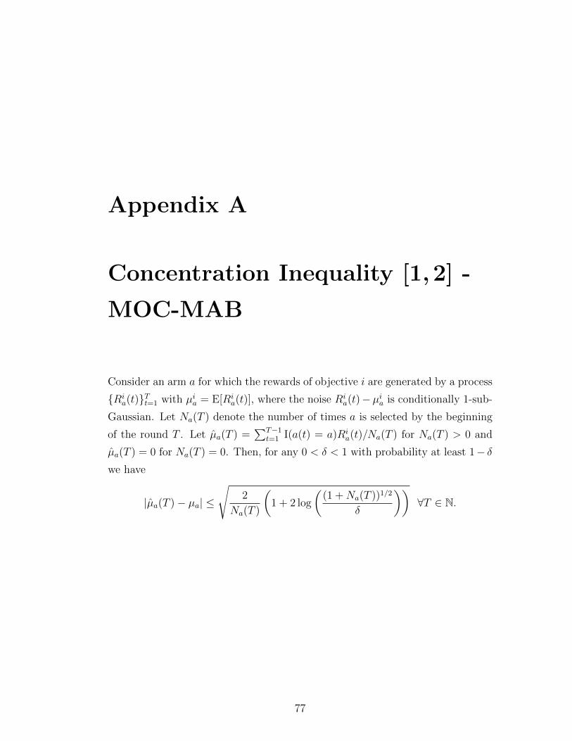
Appendix A

Concentration Inequality [1, 2] -

MOC-MAB

Consider an arm a for which the rewards of objective i are generated by a process

Ria(t)Tt=1 with µia = E[Ri

a(t)], where the noise Ria(t)−µia is conditionally 1-sub-

Gaussian. Let Na(T ) denote the number of times a is selected by the beginning

of the round T . Let µa(T ) =∑T−1

t=1 I(a(t) = a)Ria(t)/Na(T ) for Na(T ) > 0 and

µa(T ) = 0 for Na(T ) = 0. Then, for any 0 < δ < 1 with probability at least 1− δwe have

|µa(T )− µa| ≤

√2

Na(T )

(1 + 2 log

((1 +Na(T ))1/2

δ

))∀T ∈ N.

77

Appendix B

Concentration Inequality [1, 2] -

PCZ

Consider a ball B for which the rewards of objective i are generated by a process

RiB(t)Tt=1 with mean µiB = E[Ri

B(t)], where the noise RiB(t) − µiB is 1-sub-

Gaussian. Recall that B(t) is the ball selected in round t and NB(T ) is the

number of times ball B is selected by the beginning of round T . Let µiB(T ) =∑T−1t=1 I(B(t) = B)Ri

B(t)/NB(T ) for NB(T ) > 0 and µiB(T ) = 0 for NB(T ) = 0.

Then, for any 0 < θ < 1 with probability at least 1− θ we have

∣∣µiB(T )− µiB∣∣ ≤√ 2

NB(T )

(1 + 2 log

((1 +NB(T ))1/2

θ

))∀T ∈ N.

78

Appendix C

Table of Notation

79

Table C.1: Table of NotationNotation Description

xt dx-dimensional context vector observed by the learner at the be-ginning of round t

X Context setdx Number of dimensions of Xat Arm chosen by the learner at round tA Arm setda Number of dimensions of Arit Reward obtained from objective i ∈ 1, . . . , dr in round t.dr Number of objectivesrt (or rt) dr-dimensional reward vector obtained in round t, i.e. rt :=

(rit, . . . , rdrt )

µia(x) Expected reward of arm a ∈ A in objective i ∈ 1, . . . , dr, given

context x ∈ X .µa(x) (or µa(x)) dr-dimensional expected reward vector of arm a ∈ A, given con-

text x ∈ X . , i.e. µa(x) := (µia(x), . . . , µdr

a (x))κit Noise process obtained from objective i ∈ 1, . . . , dr in round t.κt (or κt) dr-dimensional noise process vector obtained in round t, i.e. κt :=

(κit, . . . , κdrt )

A∗(x) Set of arms that maximize the expected reward for the dominantobjective for context x

a∗(x) Optimal arm (for multi-objective contextual Bandit with a dom-inant objective problem formulation) given a context x ∈ X ,which is the one that maximizes the expected reward in the non-dominant objective among all arms that maximize the expectedreward in the dominant objective

O(x) Set of all Pareto optimal arms (also called the Pareto front), forgiven a particular context x,

Reg1(t) Cumulative 2D regret in the dominant objective until round tReg2(t) Cumulative 2D regret in the non-dominant objective until round

tPR(t) Cumulative Pareto regret until round t∆a(x), Pareto suboptimality gap of an arm a ∈ A given context x ∈ X .p∗ Partition such that xt ∈ p∗.P Partition setµ1a,p Sample mean of the rewards obtained from rounds prior to round

t in which the context was in p ∈ P and arm a ∈ A was selectedfor the dominant objective.

µ2a,p Sample mean of the rewards obtained from rounds prior to round

t in which the context was in p ∈ P and arm a ∈ A was selectedfor the non-dominant objective.

A∗ Candidate optimal arm set chosen by MOC-MAB

80

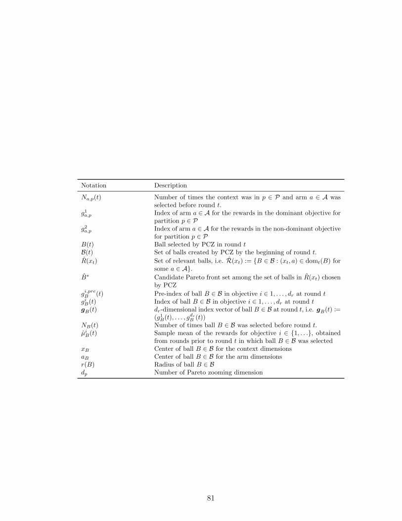
Notation Description

Na,p(t) Number of times the context was in p ∈ P and arm a ∈ A wasselected before round t.

g1a,p Index of arm a ∈ A for the rewards in the dominant objective forpartition p ∈ P

g2a,p Index of arm a ∈ A for the rewards in the non-dominant objectivefor partition p ∈ P

B(t) Ball selected by PCZ in round tB(t) Set of balls created by PCZ by the beginning of round t.

R(xt) Set of relevant balls, i.e. R(xt) := B ∈ B : (xt, a) ∈ domt(B) forsome a ∈ A.

B∗ Candidate Pareto front set among the set of balls in R(xt) chosenby PCZ

gi,preB (t) Pre-index of ball B ∈ B in objective i ∈ 1, . . . , dr at round tgiB(t) Index of ball B ∈ B in objective i ∈ 1, . . . , dr at round tgB(t) dr-dimensional index vector of ball B ∈ B at round t, i.e. gB(t) :=

(g1B(t), . . . , gdr

B (t))NB(t) Number of times ball B ∈ B was selected before round t.µiB(t) Sample mean of the rewards for objective i ∈ 1, . . ., obtained

from rounds prior to round t in which ball B ∈ B was selectedxB Center of ball B ∈ B for the context dimensionsaB Center of ball B ∈ B for the arm dimensionsr(B) Radius of ball B ∈ Bdp Number of Pareto zooming dimension

81