Lower bounds for single-machine scheduling problems
13
Lower Bounds for Single-Machine Scheduling Problems Reza H. Ahmadi University of California at Los Angeles, Los Angeles, California Uttarayan Bagchi" Department of Management, CBA 4.202, The University of Texas, Austin, Texas 78712 This article addresses deterministic, nonpreemptive scheduling of rz jobs with unequal release times on a single machine to minimize the sum of job completion times. This problem is known to be NP-hard. The article compares six available lower bounds in the literature and shows that the lower bound based on the optimal solution to the preemptive version of the problem is the dominant lower bound. Complexity studies of scheduling problems have shown that most scheduling problems in the literature are NP-hard, which makes it unlikely that polynomi- ally bounded algorithms will ever be found for any one of these probiems. That even simple-looking scheduling problems often turn out to be computational nightmares is best illustrated by the problem we consider in this article: deter- ministic, nonpreemptive scheduling of n jobs with unequal release times on a single machine to minimize the sum of job completion times. If release times are identical then the problem is solved by the well-known SPT (shortest processing time) sequencing rule (Smith [S]). When the release times are un- equal but preemption is allowed, the problem can be solved by the SRPT (shortest remaining processing time) sequencing rule (Baker [l]). If, however, the release times are unequal and preemption is not allowed, then the problem is NP-hard (Lenstra et al. [6]). Consequently, branch-and-bound algorithms for this problem have been proposed by Chandra [3] and Dessouky and Deogun [4]. The success of such an algorithm depends considerably on whether a tight lower bound to the objective function can be determined in an efficient manner. It is the purpose of this article to compare the available lower bounding proced- ures in the literature. The earliest and most straightforward lower bound is based on the SRPT solution to the preemptive version of the problem which was employed by Chandra [3]. The running time of this procedure is O(n1ogn). Dessouky and Deogun [4] obtained a lower bound in O(n2) time by partially relaxing the release times and sequencing the jobs in the order of earliest completion time. Several authors have addressed the weighted version of this problem in which each job has associated with it a positive weight and the scheduling objective is to minimize the sum of weighted completion times. Bianco and Ricciardelli [2] *To whom correspondence should be addressed. Naval Research Logistics, Vol. 37, pp. 967-979 (1990) Copyright 0 1990 by John Wiley & Sons, Inc. CCC 0028-1441/90/060967-13$04.00
-
Upload
independent -
Category
Documents
-
view
4 -
download
0
Transcript of Lower bounds for single-machine scheduling problems
Lower Bounds for Single-Machine Scheduling Problems
Reza H. Ahmadi University of California at Los Angeles, Los Angeles, California
Uttarayan Bagchi" Department of Management, CBA 4.202, The University of Texas, Austin, Texas
78712
This article addresses deterministic, nonpreemptive scheduling of rz jobs with unequal release times on a single machine t o minimize the sum of job completion times. This problem is known to be NP-hard. The article compares six available lower bounds in the literature and shows that the lower bound based on the optimal solution to the preemptive version of the problem is the dominant lower bound.
Complexity studies of scheduling problems have shown that most scheduling problems in the literature are NP-hard, which makes it unlikely that polynomi- ally bounded algorithms will ever be found for any one of these probiems. That even simple-looking scheduling problems often turn out to be computational nightmares is best illustrated by the problem we consider in this article: deter- ministic, nonpreemptive scheduling of n jobs with unequal release times on a single machine to minimize the sum of job completion times. If release times are identical then the problem is solved by the well-known SPT (shortest processing time) sequencing rule (Smith [S]). When the release times are un- equal but preemption is allowed, the problem can be solved by the SRPT (shortest remaining processing time) sequencing rule (Baker [l]). If, however, the release times are unequal and preemption is not allowed, then the problem is NP-hard (Lenstra et al. [6]). Consequently, branch-and-bound algorithms for this problem have been proposed by Chandra [3] and Dessouky and Deogun [4]. The success of such an algorithm depends considerably on whether a tight lower bound to the objective function can be determined in an efficient manner. It is the purpose of this article to compare the available lower bounding proced- ures in the literature.
The earliest and most straightforward lower bound is based on the SRPT solution to the preemptive version of the problem which was employed by Chandra [3]. The running time of this procedure is O(n1ogn). Dessouky and Deogun [4] obtained a lower bound in O(n2) time by partially relaxing the release times and sequencing the jobs in the order of earliest completion time. Several authors have addressed the weighted version of this problem in which each job has associated with it a positive weight and the scheduling objective is to minimize the sum of weighted completion times. Bianco and Ricciardelli [2]
*To whom correspondence should be addressed.
Naval Research Logistics, Vol. 37, pp. 967-979 (1990) Copyright 0 1990 by John Wiley & Sons, Inc. CCC 0028-1441/90/060967-13$04.00

968 Naval Research Logistics, Vol. 37, (1990)
4
obtained a lower bound by completely relaxing the release times and including a correction term for the job overlaps that result. The running time of their procedure is O(n’). Hariri and Potts [3] obtained a lower bound in O(n1ogn) time by performing a Lagrangian relaxation of the release time constraints. Further refinements yielded an improved lower bound with a running time of O(n2 logn). Recently, Posner [7] used job splitting to obtain a lower bound for the single-machine problem of minimizing the sum of weighted completion times subject to deadlines. Posner suggested that his lower bounding approach may also be used for the problem of minimizing the sum of weighted completion times subject to release times. This lower bounding approach has a running time of O(n logn).
We show in this article that the SRPT lower bound dominates the five other lower bounds referred to above. Because the time complexity of the SRPT lower bounding procedure is no worse than that of any of the other lower bounding procedures, it follows that the SRPT procedure is the best available. The rest of the article proceeds as follows. In Section 1 we present some notations and compute the SRPT lower bound for a numerical example. In the remaining sections we prove that the SRPT lower bound dominates the lower bound due to Dessouky and Deogun [4] the lower bound due to Bianco and Ricciardelli [3] the two lower bounds due to Hariri and Potts [5] , and the lower bound due to Posner [7].
2 3 1
1. PRELIMINARIES
The problem considered in this article say ( P ) , may be described as follows. A single machine is immediately available for processing n jobs (numbered 1,2, . . . ,n), one job at a time. Each job i, i = 1,2, . . . ,n is available for process- ing at its release time r , , has a processing time pi, and once. started must be processed without interruption. Without any loss of generality, we assume that the minimum release time is zero. Let C, be the completion time of job i. The objective is to determine a schedule of n jobs such that Z:=, C, is minimized.
Consider the following four-job example which will be used throughout the article :
i 1 2 3 4 Ti 0 2 5 1 Pi 5 1 1 3
The optimal schedule can be shown to be the following:
0 1 4 5 6 11 . The optimal sum of completion times is (4 + 5 + 6 + 11) = 26. Suppose now
that preemption is allowed. The optimal schedule obtained by using the SRPT scheduling rule is the following:

Ahmadi and Bagchi: Single-Machine Scheduling 969
0 1 2 3 5 6 10
The sum of completion times in the SRPT schedule is (3 + 5 + 6 + 10) = 24. The optimal solution under preempt-resume mode must be a lower bound on the optimal solution when preemption is not allowed. Thus the sum of com- pletion times in the SRPT schedule is a lower bound for (P) . We denote this bound by SRPTLBD. For the numerical example under consideration we have SRPTLBD = 24.
2. THE LOWER BOUND DUE TO DESSOUKY AND DEOGUN
Dessouky and Deogun [4] derived a lower bound for ( P ) by determining an earliest completion time (ECT) schedule with the release times partially relaxed. An ECT schedule is formed by scheduling jobs as early as possible in their order of processing where the next job to be scheduled has the earliest com- pletion time of all unscheduled jobs. Ties are broken by choosing the job with the earliest start time. Further ties are broken by choosing job i with minimum i. The ECT schedule is then modified to yield a lower bound. This modification does not change the sequence of jobs in the ECT schedule, but may change their start times. Each job in the modified ECT schedule is started at the completion time of the preceding job in the modified ECT schedule, or at the minimum release time of all unscheduled jobs, including itself, whichever is greater. The sum of the completion times in the modified ECT schedule, referred to as the DD schedule, is a lower bound for ( P ) . Let this lower bound be denoted by DDLBD.
The ECT schedule for the four-job example is
job 2 4 3 1 start time 2 3 6 7
completion time 3 6 7 12
The DD schedule is:
job 2 4 3 1 start time 0 1 4 5
completion time 1 4 5 10
which yields DDLBD = (1 + 4 + 5 + 10) = 20, as compared to SRPTLBD = 24.
THEOREM 1: For any instance of (P), SRPTLBD 2 DDLBD.
PROOF: See the appendix.
3. THE LOWER BOUND DUE TO BIANCO AND RICCIARDELLI
The lower bound due to Bianco and Ricciardelli [2], denoted by BRLBD, can be written as
970 Naval Research Logistics, Vol. 37, (1990)
n n--l "I
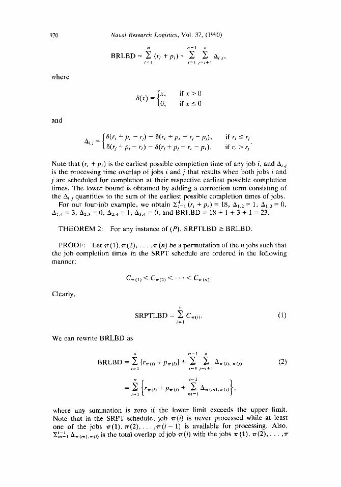
BRLBD = x ( r j + p i ) + 2- 2 Ai , i , i= 1 i = l / = i t 1
where
and
Note that ( r , + p i ) is the earliest possible completion time of any job i , and is the processing time overlap of jobs i and j that results when both jobs i and j are scheduled for completion at their respective earliest possible completion times. The lower bound is obtained by adding a correction term consisting of the A i j quantities to the sum of the earliest possible completion times of jobs.
For our four-job example, we obtain C;='=, (ri + p i ) = 18, At,* = 1, A l , 3 = 0, A1,4 = 3, A2,3 = 0, A2,4 = 1, A3,4 = 0, and BRLBD = 18 + 1 + 3 + 1 = 23.
THEOREM 2: For any instance of ( P ) , SRPTLBD 2 BRLBD.
PROOF: Let ~(1) ,7r (2) , . . . ,7r(n) be a permutation of the n jobs such that the job completion times in the SRPT schedule are ordered in the following manner:
Clearly,
n
SRPTLBD = 2 CT(;) . i = 1
We can rewrite BRLBD as
" n-1 n
where any summation is zero if the lower limit exceeds the upper limit. Note that in the SRPT schedule, job ~ ( i ) is never processed while at least one of the jobs ~ ( l ) , 7r(2), . , . , ~ ( i - 1) is available for processing. Also, xi- 1
m=l Am(m) ,n ( i ) is the total overlap of job ~ ( i ) with the jobs ~ ( l ) , 7r(2), . . . ,7r
Ahmadi and Bagchi: Single-Machine Scheduling
( i - 1). It follows that
i- 1
97 1
From (1)-(3) we obtain SRPTLBD 2 BRLBD.
4. THE LOWER BOUNDS DUE TO HARIRL AND POTTS
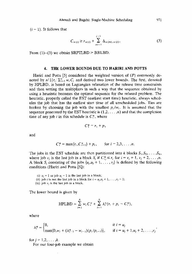
Hariri and Potts [5 ] considered the weighted version of ( P ) commonly de- noted by n ( 1 Jri I Xye1 wi Ci and derived two lower bounds. The first, denoted by HPLBD, is based on Lagrangian relaxation of the release time constraints and then setting the multipliers in such a way that the sequence obtained by using a heuristic becomes the optimal sequence for the relaxed problem. The heuristic, properly called the EST (earliest start time) heuristic, always sched- ules the job that has the earliest start time of all unscheduled jobs. Ties are broken by choosing the job with the smallest p i /wi . It is assumed that the sequence generated by the EST heuristic is (1,2, . . . ,n) and that the completion time of any job i in this schedule is C ? , where
and
C? = max{ri,C?-l} +pi, for i = 2,3,. . . ,n.
The jobs in the EST schedule are then partitioned into k blocks SlrS2, . . . , S k , where job v, is the last job in a block S, if C$, 5 ri for i = v, + 1, vj + 2, . . . ,~t.
A block S, consisting of the jobs {uj,u, + 1, . . . , v j } is defined by the following conditions (Hariri and Potts [5]):
(i) u, = 1 or job ii, - 1 is the last job in a block; (ii) job i is not the last job in a block for i = u,,u, + 1, . . . ,v, - 1:
(iii) job v, is the last job in a block.
The lower bound is given by
n n
HPLBD = E wiC? + 2 AF(rj + p i - CF), i = 1 i= 1
where
A: = {” if i = uj
if i = uj + l ,uj + 2 , . . . , v j ’ max{O,wi + - ~ ~ - ~ ) ( p ~ / p ~ - J } ,
for J = 1,2, . . . ,k . For our four-job example we obtain

912, Naval Research Logistics, Vol. 37, (1990)
C? = 5 , C 3 = 6 , C g = 7 , C$=lO, ~ 1 ~ 4 ; AT = 0, A 3 = 415, A S = 4f5, AX = 215,
and
HPLBD = ( 5 + 6 + 7 + 10) + (0)(5 - 5 ) + (4/5)(3 - 6)
+ (4/5)(6 - 7) + (2/5)(4 - 10)
= 28 - (1215 + 4/5 + 12/5)
= 22.4.
The second bound due to Hariri and Potts, denoted by IHPLBD, is an improvement on HPLBD and is based on the A,*. The jobs in the EST schedule are now reordered within each block in nondecreasing order of A T to give a permutation T = [T ( l ) , ~ (2), . , . ,T (n)] such that S, = {T ( u , ) , ~ (u, + l ) , . . . ,T
(v,)} and A * , ( , ) I I - I A*,cv , ) for all j . Further definitions include the following:
S(h) = Si(h-’) - { r ( u j + h - l)}, for h = 1,2, . . . ,vj - u j ; j = 1,2, . . . ,k , Si(0) = S,
pjh) = A* W ( U , + h ) - A*, (u j+h- l ) , for h = 1,2, . , . ,vj - uj; j = 1,2, . . . , k ,
bjh’ = c ( l i +Pi), i E sjh’
for h = 1,2, . . . ,vj - uj; j = 1,2, . . . ,k.
Also p(h) denotes the sum of completion times for the jobs in when they are sequenced according to the SRPT rule, for h = 1,2, . . . ,vj - u j ; j = 1,2 , . . . , k . The second lower bound is written as
where it is assumed that any summation is zero when its lower limit exceeds its upper limit.
For our four-job example we obtain
IHPLBD = 22.4 + (2/5)(14 - 13) + (2/5)(9 - 9) + (0)(6 - 6)
= 22.8.
Ahmadi and Bagchi: Single-Machine Scheduling 973
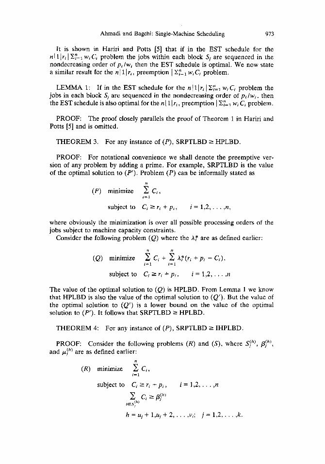
It is shown in Hariri and Potts [S ] that if in the EST schedule for the nllIri 1 XY='=, wiCi problem the jobs within each block S j are sequenced in the nondecreasing order of p i /wi then the EST schedule is optimal. We now state a similar result for the n 11 I r i , preemption I Z;==, wi Ci problem.
LEMMA 1: If in the EST schedule for the n 11 1 ri I XY=l wi Ci problem the jobs in each block Sj are sequenced in the nondecreasing order of p i / w i , then the EST schedule is also optimal for the n I 1 I ri, preemption 1 XY='=, wi Ci problem.
PROOF: The proof closely parallels the proof of Theorem 1 in Hariri and Potts [5] and is omitted.
THEOREM 3. For any instance of (P), SRPTLBD 2 HPLBD.
PROOF: For notational convenience we shall denote the preemptive ver- sion of any problem by adding a prime. For example, SRPTLBD is the value of the optimal solution to ( P ' ) . Problem (P) can be informally stated as
n
(PI minimize X ci, i= 1
subject to Ci L ri + pi, where obviously the minimization is over all jobs subject to machine capacity constraints.
Consider the following problem (Q) where
i = 1,2, . . . ,n,
possible processing orders of the
the A T are as defined earlier:
n n
(Q) minimize Ci + Af(ri + p i - Ci),
subject to Ci 2 ri + p i ,
i = 1 i= 1
i = 1,2, . , . ,n
The value of the optimal solution to (Q) is HPLBD. From Lemma 1 we know that HPLBD is also the value of the optimal solution to (Q'). But the value of the optimal solution to (Q') is a lower bound on the value of the optimal solution to (P'). It follows that SRPTLBD 2 HPLBD.
THEOREM 4: For any instance of ( P ) , SRPTLBD L IHPLBD.
PROOF: Consider the following problems ( R ) and ( S ) , where Sjh), @(", and pjh) are as defined earlier:
n
( R ) minimize E ci, i = 1
subject to Ci 2 ri + p i , i = 1,2, . . . ,n
h = uj + l,uj + 2, . . . ,vj; j = 1,2, . . . ,k .
974 Naval Research Logistics, Vol. 37, (1990)
k v - u I 1
i= 1 j = I h = l
subject to Ci 2 ri + p i , i = 1,2, . . . ,n.
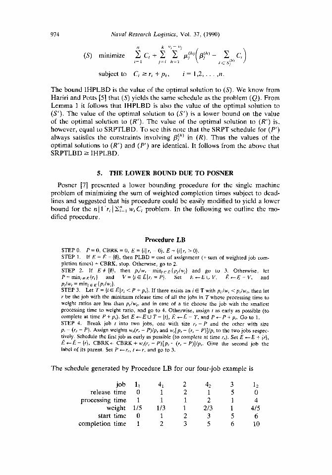
The bound IHPLBD is the value of the optimal solution to ( S ) . We know from Hariri and Potts [5] that (S) yields the same schedule as the problem (Q). From Lemma 1 it follows that IHPLBD is also the value of the optimal solution to (S’). The value of the optimal solution to ( S ’ ) is a lower bound on the value of the optimal solution to (R‘) , The value of the optimal solution to (R‘) is, however, equal to SRPTLBD. To see this note that the SRPT schedule for ( P ’ ) always satisfies the constraints involving pjh’ in ( R ) . Thus the values of the optimal solutions to (R’) and (P’) are identical. It follows from the above that SRPTLBD B IHPLBD.
5. THE LOWER BOUND DUE TO POSNER
Posner [7] presented a lower bounding procedure for the single machine problem of minimizing the sum of weighted completion times subject to dead- lines and suggested that his procedure could be easily modified to yield a lower bound for the n 11 1 ri 1 C$, wi Ci problem. In the following we outline the mo- dified procedure.
Procedure LB STEP 0. P = 0, CBRK = 0, E = {il rr = O}, E = {iI r, > 0). STEP 1. If E = E = {0}, then PLBD = cost of assignment (=sum of weighted job com- pletion times) + CBRK, stop. Otherwise, go to 2. STEP 2. If E # {0}, then p , / w , = min,,E{p,/w,} and go to 3. Otherwise, let P=min, ,E{rr} and V = { i E E ‘ ( r , = P } . Set E c E U V , E c E - V , and pdw, = min, E 6 {p,/w,}. STEP 3. Let T = {i E Elr, < P + pt}. If there exists an i E T with p 2 /w , < p,/w,, then let r be the job with the minimum release time of all the jobs in T whose processing time to weight ratios are less than p,lw,, and in case of a tie choose the job with the smallest processing time to weight ratio, and go to 4. Otherwise, assign t as early as possible (to complete at time P + p,). Set E +-E U T - {f}, E +-E - T , and P t P + p,. Go to 1. STEP 4. Break job f into two jobs, one with size rr - P and the other with size pr - (r , - P ) . Assign weights w,(r, - P ) / p , and w,[p, - (r , - P ) ] / p , to the two jobs respec- tively. Schedule the first job as early as possible (to complete at time rr). Set E c E + (r}, 6 - {r}, CBRK +- CBRK + wt(r, - P ) [ p , - (rr - P ) ] / p , . Give the second job the label of its parent. Set P e r , , t c r , and go to 3.
The schedule generated by Procedure LB for our four-job example is
job l1 41 2 42 3 1 2 release time 0 1 2 1 5 0
processing time 1 1 1 2 1 4 weight 1/5 113 1 213 1 415
start time 0 1 2 3 5 6 completion time 1 2 3 5 6 10

Ahmadi and Bagchi: Single-Machine Scheduling 975
The resulting lower bound is
PLBD = ((1/5)(1) + (1/3)(2) + (1)(3) + (2/3)(5) + (1)(6)
+ (4/5)(10)) + ((1)(1)(4)/5 + (1)(1)(2)/3) = 21.2 + 22/15
= 22:. 2
Let Z ( u ) be the sum of weighted completion times in any schedule a. Let u* denote the optimal schedule for ( P ) .
THEOREM 5:
PROOF:
For any instance of ( P ) , Z (u*) 2 PLBD.
The proof closely parallels the proof of Proposition 5 in Posner [7]. Let (Pl) be the scheduling problem generated by Procedure LB, with the additional jobs and new processing times and weights, and let v1 be the schedule generated by Procedure LB for (P) . Suppose that a job t of ( P ) is broken by Procedure LB into k pieces. Assume that the same job t in u* is broken into k pieces to match the processing times, weights, and sequencing order of these pieces in vl. Of course, these pieces are contiguous in CT*. When this analysis is repeated for each job broken by Procedure LB, we get a feasible schedule for (P l ) by breaking the jobs in u* . Let this schedule be vz. From the proof of Proposition 5 in Posner, we can write
Z(U*) = Z ( V ~ ) + CBRK(u*, y),
where CBRK(a*, v2) is the cost associated with deriving vz from u*. Further- more, we have
PLBD = Z ( V ~ ) + CBRK(u*, ~ 1 ) .
Clearly, CBRK(u*, y) = CBRK(a*, vl). It follows that to prove Theorem 5 , we need to show that Z( vz) 2 Z( vl). This is accomplished by proving that v1 is optimal for (Pl) .
Suppose that each job i in (P l ) is broken into pi unit size pieces, each with a weight w i /pi and a release time ri. The resulting procedure, denoted by (E), is the problem of scheduling unit processing time jobs with release times to minimize the sum of weighted completion times. It is easily shown that the optimal schedule for (P2) is obtained by scheduling jobs as early as possible, breaking ties by choosing the next job to be scheduled that has the minimum processing time to weight ratio among all immediately available jobs. It is easily verified that in the optimal schedule for (P2), say y, all the pi pieces of job i of (P l ) are contiguously placed and the set of these pieces is scheduled at the same time as job i in vl. Clearly, Z(vJ = Z(v3) + CBRK(vl, v3), and the preceding discussion concerning the breaking of jobs implies that v1 is optimal for (Pl) . It follows that Z(a*) 2 PLBD.
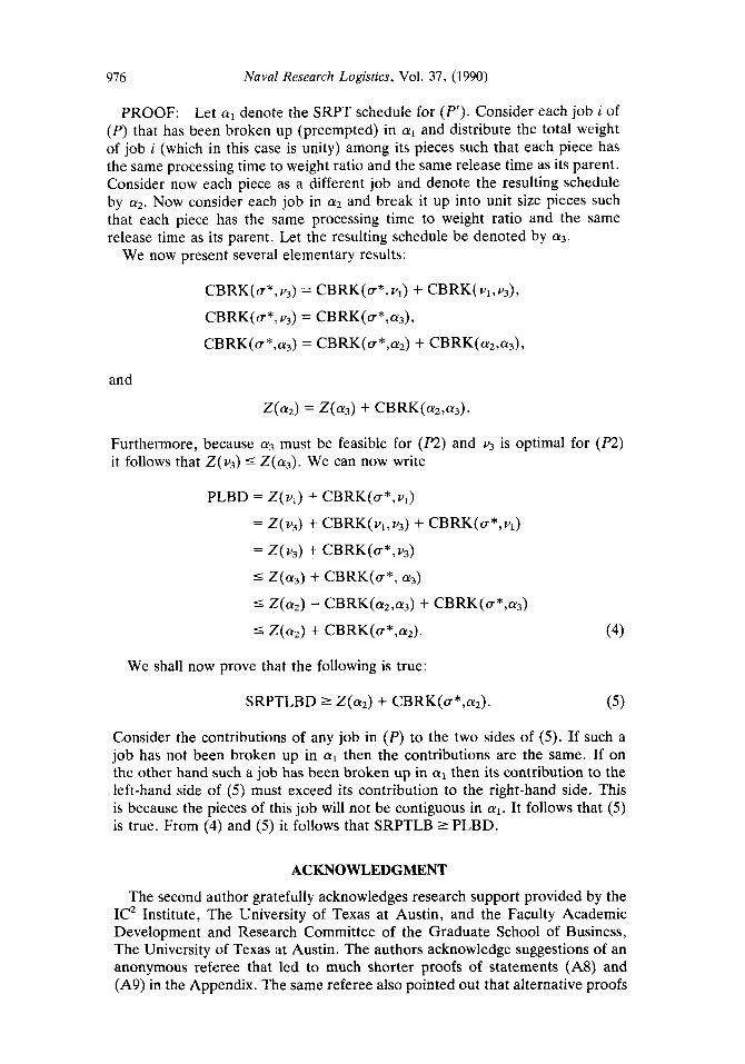
THEOREM 6: For any instance of ( P ) , SRPTLB L PLBD.
976 Naval Research Logistics, Vol. 37, (1990)
PROOF: Let a1 denote the SRPT schedule for (P’) . Consider each job i of ( P ) that has been broken up (preempted) in a1 and distribute the total weight of job i (which in this case is unity) among its pieces such that each piece has the same processing time to weight ratio and the same release time as its parent. Consider now each piece as a different job and denote the resulting schedule by a2. Now consider each job in a2 and break it up into unit size pieces such that each piece has the same processing time to weight ratio and the same release time as its parent. Let the resulting schedule be denoted by a3.
We now present several elementary results:
CBRK(C*,V~)= CBRK(a*,y) + CBRK(V~,V~) ,
C B R K ( ~ * , V ~ ) = CBRK(a*,a3),
CBRK(a*,a3) = CBRK(U*,(Y~) + CBRK(aZ,a3),
and
Furthermore, because a3 must be feasible for (P2) and v3 is optimal for (P2) it follows that Z(v3) 5 Z ( a 3 ) . We can now write
PLBD = Z ( v l ) + CBRK(a*,v,)
= Z ( y ) + CBRK(vl,v3) + CBRK(a*,vl)
= Z ( v 3 ) + CBRK(a*,v3)
I Z ( a 3 ) + CBRK(a*, a3)
5 Z(a2) - CBRK(a2,.3) + CBRK(U*,(U~)
5 Z ( ( Y ~ ) + CBRK(U*,(Y~). (4)
We shall now prove that the following is true:
SRPTLBD Z Z(a2) + CBRK(a*,az). ( 5 )
Consider the contributions of any job in ( P ) to the two sides of (5 ) . If such a job has not been broken up in a1 then the contributions are the same. If on the other hand such a job has been broken up in a1 then its contribution to the left-hand side of (5 ) must exceed its contribution to the right-hand side. This is because the pieces of this job will not be contiguous in aI. It follows that ( 5 ) is true. From (4) and ( 5 ) it follows that SRPTLB 2 PLBD.
ACKNOWLEDGMENT
The second author gratefully acknowledges research support provided by the IC2 Institute, The University of Texas at Austin, and the Faculty Academic Development and Research Committee of the Graduate School of Business, The University of Texas at Austin. The authors acknowledge suggestions of an anonymous referee that led to much shorter proofs of statements (A8) and (A9) in the Appendix. The same referee also pointed out that alternative proofs
Ahmadi and Bagchi: Single-Machine Scheduling 977
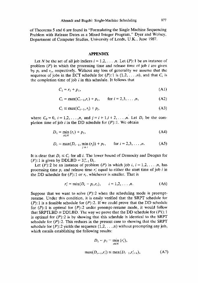
of Theorems 5 and 6 are found in “Formulating the Single Machine Sequencing Problem with Release Dates as a Mixed Integer Program,” Dyer and Wolsey, Department of Computer Studies, University of Leeds, U.K., June 1987.
APPENDIX
Let N be the set of all job indices i = 1,2, . . . ,n. Let ( P ) : 1 be an instance of problem ( P ) in which the processing time and release time of job i are given by p i and r i , respectively. Without any loss of generality we assume that the sequence of jobs in the ECT schedule for (P):l is (1,2, . . . ,n), and that Ci is the completion time of job i in this schedule. It follows that
Ci 5 max(CiPl, rj) + p i , (A31
where C, = 0, i = 1,2, . . . ,n, and j = i + 1,i + 2 , . . . ,n. Let Di be the com- pletion time of job i in the DD schedule for ( P ) : 1. We obtain
D1 = min ( r i ) + pl, (‘44) E N
Di = max(Di--l, min ( r j ) ) + p i , for i = 2,3, . . . ,n. (A51 jzi
It is clear that D j 5 Ci for all i. The lower bound of Dessouky and Deogun for (P):l is given by DDLBD = CY==, Di.
Let (P):2 be an instance of problem ( P ) in which job i, i = 1 , 2 , . . , ,n, has processing time pi and release time rl equal to either the start time of job i in the DD schedule for ( P ) : 1 or r i , whichever is smaller. That is
rl = min(Di - p i , r , ) , i = 1,2, . . . ,n. (A6)
Suppose that we want to solve (P):2 when the scheduling mode is preempt- resume. Under this condition, it is easily verified that the SRPT schedule for (P):l is a feasible schedule for (P):2. If we could prove that the DD schedule for (P):l is optimal for (P):2 under preempt-resume mode, it would follow that SRPTLBD r DDLBD. The way we prove that the DD schedule for (Pl): 1 is optimal for (P):2 is by showing that this schedule is identical to the SRPT schedule for (P):2. This reduces in the present case to showing that the SRPT schedule for (P):2 yields the sequence (1,2, . . .,n) without preempting any job, which entails establishing the following results:
D~ - p1 = min (rl), i E N
978 Naval Research Logistics, Vol. 37, (1990)
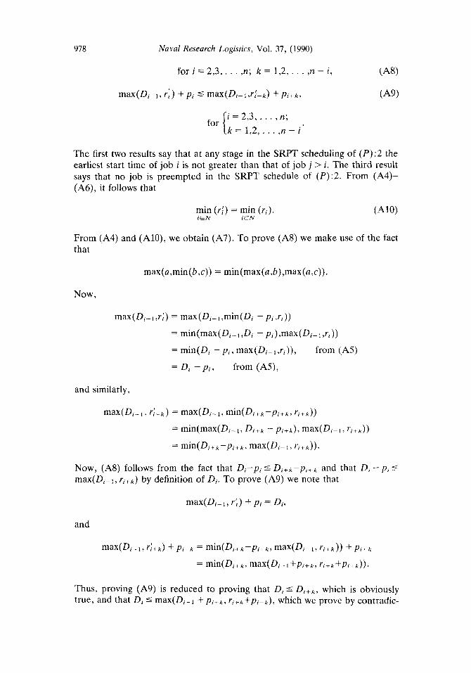
for i = 2,3, , . . ,n; k = 1,2,. . . ,n - i ,
max(Di- I , r l ) -t p i -i max(Di- 1 ,rftk) + p i + k ,
i = 2,3, . . . ,n; k = 1,2,. . . ,n - i
for [ The first two results say that at any stage in the SRPT scheduling of ( P ) : 2 the earliest start time of job i is not greater than that of job j > i . The third result says that no job is preempted in the SRPT schedule of ( P ) : 2 . From (A4)- (A6), it follows that
min (rf) = min (Y;). i E N ; E N
From (A4) and (AlO), we obtain (A7). To prove (A8) we make use of the fact that
max(a,min( b,c)) = min(max(a,b) ,max(a,c)).
Now,
max(Di-l,ril) = max(Di-l,min(Di - p i , r , ) )
= min(max(Di-,,Di - pi),max(Dj-l,r,))
= min(Dj - p i , max(Di-l,r,)),
- D, - p i ,
from (A5) - from (A5),
and similarly,
max(Di-,, r , ! + k ) = max(Dj-l, min(Di+k-pi+k, r i t k ) )
= min(max(Di-.,, Ditk - p i + k ) , max(DIpI , r i t k ) )
= min(Di+k-pi+k, max(Di-l, r i + d ) .
Now, (A8) follows from the fact that Dj-pi 5 D i + k - p i + k and that Di - p i I max(Di-I, r j t k ) by definition of Di. To prove (A9) we note that
max(Dj-l, r : ) + p i = Di,
and
Thus, proving (A9) is reduced to proving that Dj 5 Di+k, which is obviously true, and that Di 5 max(Di-l + p i + k r ri+k+pi+k), which we prove by contradic-
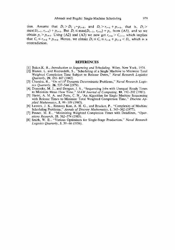
Ahmadi and Bagchi: Single-Machine Scheduling 979
tion. Assume that Di > Di-- l+pi+k, and Di > ri+k + P i + k , that is, Di > max(Di-l, r i + k ) + P i + k . But Di 5 max(DiPl, ri+J + p i , from (A5), and so we obtain p i > P i t k . Using (A2) and (A3) we now get r i f k > Ci-, , which implies that Ci 5 + P i t k . Hence, we obtain Di 5 Ci 5 ri+k + P i t k < Di, which is a contradiction.
REFERENCES [l] Baker,K. R. , Introduction to Sequencing and Scheduling. Wiley, New York, 1974. [2] Bianco, L. and Ricciardelli, S., “Scheduling of a Single Machine to Minimize Total
Weighted Completion Time Subject to Release Dates,” Naval Research Logistics Quarterly, 29, 151-167 (1982)
[3] Chandra, R., “On nll lE Dynamic Deterministic Problems,” Naval Research Logis- tics Quarterly, 26, 537-544 (1979).
[4] Dessouky, M. I . , and Deogun, J. S . , “Sequencing Jobs with Unequal Ready Times to Minimize Mean Flow Time,” SZAM Journal of Computing, 10, 192-202 (1981).
[5] Hariri, A. M. A. and Potts, C. N., ‘An Algorithm for Single Machine Sequencing with Release Times to Minimize Total Weighted Completion Time,” Discrete A p - plied Mathematics, 5 , 99-109 (1983).
[6] Lenstra, J. K., Rinnooy Kan, A. H. G., and Brucker, P., “Complexity of Machine Scheduling Problems,” Annals of Discrete Mathematics, 1, 343-362 (1977).
[7] Posner, M. E., “Minimizing Weighted Completion Times with Deadlines, “Oper- ations Research, 33, 562-574 (1985).
[8] Smith, W. E., “Various Optimizers for Single-Stage Production,” Naval Research Logistics Quarterly, 3, 59-66 (1956).