arX

iv:m

ath/

0210

016v

1 [

mat

h.PR

] 1

Oct

200

2

LOWER BOUNDS FOR BOUNDARY ROUGHNESS

FOR DROPLETS IN BERNOULLI PERCOLATION

HASAN B. UZUN AND KENNETH S. ALEXANDER

Abstract. We consider boundary roughness for the “droplet” created when su-percritical two-dimensional Bernoulli percolation is conditioned to have an opendual circuit surrounding the origin and enclosing an area at least l

2, for large l.The maximum local roughness is the maximum inward deviation of the dropletboundary from the boundary of its own convex hull; we show that for large l thismaximum is at least of order l

1/3(log l)−2/3. This complements the upper bound oforder l

1/3(log l)2/3 proved in [Al3] for the average local roughness. The exponent1/3 on l here is in keeping with predictions from the physics literature for interfacesin two dimensions.

1. Introduction

We consider Bernoulli bond percolation on the square lattice at supercritical den-sity, conditioned to have a large dual circuit enclosing the origin; we denote theoutermost such circuit by Γ0. (Complete definitions and the basic properties of themodel will be given in the next section.) The supercritical, or percolating, regimeof Bernoulli percolation is the analog of the low-temperature phase of a spin sys-tem, and the region enclosed by the dual circuit is the analog of the droplet thatoccurs with high probability in the Ising magnet below the critical temperature in afinite box with minus boundary condition, when it is conditioned to have a numberof plus spins somewhat larger than is typical [DKS]. In fact, the droplet boundaryin the Ising magnet appears as a circuit of open dual bonds in the correspondingFortuin-Kastelyn random cluster model (briefly, the FK model) of [FK], in view ofthe construction given in [ES]. One can gain information for the study of the Isingdroplet by studying the FK model conditioned on Γ0 enclosing at least a given areal2, as is done in [Al3]. The droplet boundary in this FK model thus corresponds toan interface; the heuristics in the case of Bernoulli percolation are the same, but themathematics is more tractable. We therefore refer to Γ0 and its interior as a droplet.Our main result is a lower bound on the maximum local roughness of the droplet, that

Date: February 1, 2008.1991 Mathematics Subject Classification. Primary: 60K35; Secondary: 82B20, 82B43.Key words and phrases. droplet, interface, local roughness.The research of the first author was supported by NSF grant DMS-9802368. The research of the

second author was supported by NSF grants DMS-9802368 and DMS-0103790.1

2 HASAN B. UZUN AND KENNETH S. ALEXANDER

is, the maximum inward deviation of the boundary of the droplet from the boundaryof its convex hull. Related upper bounds were proved in [Al3].

The study of the shapes of such droplets is related to a classical problem: Whena fixed volume of one phase is immersed in another, what is the equilibrium shapeof the droplet, or crystal, having minimal surface tension? When the surface tensionis known, this is an isoperimetric problem. The solution of the continuum version ofthe problem is given by Wulff [Wu]: Let τ(n) be the surface tension of a flat interfaceorthogonal to the outward normal n. For a fixed crystal volume, the equilibriumshape is given by the convex set

W = {x ∈ Rd | x · n ≤ τ(n), for all n}.(1.1)

In the two-dimensional Ising model, say with minus boundary condition and condi-tioned to have an excess of pluses, a rigorous justification of the Wulff constructionhas been given for the resulting droplet of plus phase. Minlos and Sinai considered aninstance in which the temperature T tends to zero as the volume grows to infinity, andproved that most of the excess plus spins form a single droplet of essentially squareshape ([MS1], [MS2]); the Wulff shape W also tends to a square as T → 0. Dobrushin,Kotecky and Shlosman [DKS] then provided a justification of the Wulff constructionat very low fixed temperatures. Moreover, they showed that the Hausdorff distancebetween the droplet boundary γ and the boundary of the Wulff shape W is boundedby a power of the linear scale of the droplet. This Hausdorff distance is related butnot equivalent to local roughness; see [Al3]. The very-low-temperature restriction wasremoved by Ioffe and Schonmann [IS], who proved Dobrushin-Kotecky-Schlosman the-orem up to the critical temperature. For Bernoulli percolation the Wulff constructionwas justified in [ACC], and for the FK model this was done in [Al3]. For these modelsthe surface tension is given by the inverse of the exponential rate of decay of the dualconnectivity.

Boundary roughness has been a topic of considerable interest in the physics litera-ture (see e.g. [KS]). The heuristics for the local roughness of Γ0, described in [Al3],are related to the boundary-roughness heuristics for two-dimensional growth mod-els such as first-passage percolation that are believed to be governed by the “KPZ”theory ([KPZ], [LNP], [NP]), to polymers in two-dimensional random environments[Pi], and, as noted in [Al3], to the heuristics of rigorously proved results on longestincreasing subsequences of random permutations [BDJ], which in turn are related tothe fluctuations of eigenvalues of random matrices (see [Jo]). In all cases for an objectof linear scale l there is known or believed to be roughness of order l1/3 and a lon-gitudinal correlation length of order l2/3. In the percolation droplet this correlationlength should appear as the typical separation between adjacent extreme points ofthe convex hull of Γ0.

In [Al3] the average local roughness, denoted ALR(Γ0), for the percolation dropletwas defined as the area between the droplet and its convex hull boundary, dividedby the Euclidean length of the convex hull boundary. It was proved there that with

LOWER BOUNDS FOR BOUNDARY ROUGHNESS 3

high probability, for a droplet conditioned to have area at least l2, the ALR(Γ0) isO(l1/3(log l)2/3). The main feature of interest is the exponent 1/3 matching the KPZheuristic; the power of log l may be considered an artifact of the proof. Here weconsider not average but maximum local roughness, denoted MLR(Γ0) and defined asthe maximum distance from any point of Γ0 to the convex hull boundary, and we showthat for the Bernoulli percolation droplet, for some c0 > 0, with high probability it isat least c0l

1/3(log l)−2/3. It was proved in [Al3] that with high probability MLR(Γ0) isO(l2/3(log l)1/3), but this is a presumably a very crude bound, lacking the right powerof l; it is more reasonable to compare the lower bound here on MLR(Γ0) to the upperbound for ALR(Γ0), as the two should differ by at most a multiplicative factor thatis a power of log l, as we explain next.

One way to obtain more-detailed heuristics for the droplet boundary is to viewit as having Gaussian fluctuations about a fixed Wulff shape of area l2, a point ofview justified in part by the results in [DH] and [Hr]. This point of view suggeststhat if we take a Brownian bridge on [0,1], rescale it by 2πl horizontally and l1/2

vertically, and wrap it around a circle of radius l, joining (0, 0) and (2πl, 0), the resultshould resemble the droplet boundary. In [Uz] it was proved that for this wrappedBrownian bridge the maximum local roughness is with high probability boundedbetween c1l

1/3(log l)2/3 and c2l1/3(log l)2/3 for some 0 < c1 < c2 < ∞. The exponent

2/3 on log l here is related to the Levy modulus of continuity for Brownian motion.The wrapped-Brownian-bridge heuristic suggests that ALR(Γ0) should be of orderl1/3, without a power of log l, supporting the idea that ALR(Γ0) and MLR(Γ0) differby only a multiplicative factor that is roughly a power of log l. The circle providesa reasonable heuristic here because Ioffe and Schonmann [IS] showed that for fixed pthe curvature of the boundary of the unit-area Wulff shape is bounded away from 0and ∞.

2. Definitions, Preliminaries, Statement of Main Result

A bond, denoted 〈xy〉, is an unordered pair of nearest neighbor sites x, y ∈ Z2. Theset of all bonds between the nearest neighbor sites of Z2, will be denoted by B2. Let{ω(b), b ∈ B2} be an i.i.d. family of Bernoulli random variables with P (ω(b) = 1) = p.Given a realization of ω, a bond b ∈ B2 is said to be open if ω(b) = 1 and closedif ω(b) = 0. Consider the random graph containing the vertex set of Z2 and theopen bonds only; the connected components of this graph are called open clusters.For p below the critical probability pc = 1/2 [Ke] all open clusters are finite withprobability one and when p > pc, there exists a unique infinite cluster of open bondswith probability one.

For x ∈ Z2 let x∗ denote x + (1/2, 1/2). The lattice with vertex set {x∗ : x ∈ Z2}and all nearest neighbor bonds is called the dual lattice. Each bond b has a uniquedual bond, denoted b∗, which is its perpendicular bisector; b∗ is defined to be openprecisely when b is closed, so that the dual configuration is Bernoulli percolation at

4 HASAN B. UZUN AND KENNETH S. ALEXANDER

density 1−p. A (dual) path is a sequence (x0, 〈x0x1〉, x1, · · · , 〈xn−1, xn〉) of alternating(dual) sites and bonds. A (dual) circuit is a path with xn = x0 which has all bondsdistinct and does not cross itself (in the obvious sense). Note we allow a circuit totouch itself without crossing, i.e. nondistinct sites are not restricted to xn = x0. Fora (dual) circuit γ, the interior Int(γ) is the union of the bounded components of thecomplement of γ in R2. An open dual circuit γ is called an exterior dual circuit ina configuration ω if γ ∪ Int(γ) is maximal among all open dual circuits in ω. A sitex is surrounded by at most one exterior dual circuit; when this circuit exits, it isdenoted by Γx. | · | denotes the Euclidean norm for vectors, cardinality for finite setsand Lebesgue measure for regions in R2, depending on the context. For x, y ∈ R2, letdist(·, ·) and diam(·) denote Euclidean distance and Euclidean diameter, respectively.Let Br(x), denote the open Euclidean ball of radius r about x. For A, B ⊂ R2, definedist(A, B) = inf{dist(x, y) : x ∈ A, y ∈ B} and dist(x, A) =dist({x}, A). We definethe average local roughness of a circuit γ by

ALR(γ) =|Co(γ) \ Int(γ)||∂Co(γ)| ,

where Co(·) denotes the convex hull. The maximum local roughness is

MLR(γ) = sup{dist(x, ∂Co(γ)) : x ∈ γ}

Throughout the paper, K1, K2, ... represent constants which depend only on p. Ourmain result is the following.

Theorem 2.1. Let 1/2 < p < 1. There exists K1 > 0 such that, under the measureP(·∣∣ | Int(Γ0)| ≥ l2

), with probability approaching 1 as l →∞ we have

MLR(Γ0) ≥ K1l1/3(log l)−2/3(2.1)

The main ingredients of the proof will be coarse graining concepts, the renewalstructure of long dual connections in the supercritical regime and exchangeabilityof the increments between regeneration points, all of which will be discussed below.The basic idea is that MLR(Γ0) < K1l

1/3(log l)−2/3 implies that Γ0 stays in a narrowtube along its own convex hull, which is a highly unlikely event, due to the Gaussianfluctuations of connectivities. More precisely, if w and w′ are extreme points of Co(Γ0)separated by a distance of order l2/3(log l)−1/3, then MLR(Γ0) < K1l

1/3(log l)−2/3

requres that Γ0 stay confined within O(l1/3(log l)−2/3) of the straight line from wto w′. Gaussian fluctuations, though, would say that the typical deviation from thestraight line is of order l1/3(log l)−1/6, which is the square root of the length of the line.Thus the confinement for the segment between w and w′ is analogous to keeping themaximum magnitude of a Brownian bridge below O((log l)−1/2), and such confinementalong the entire boundary of Γ0 is very unlikely. The Brownian bridge analogy is anunderlying heuristic but does not enter directly into our proofs.

LOWER BOUNDS FOR BOUNDARY ROUGHNESS 5

We use some notation, results and techniques introduced in [Al3]. For a familyof bond percolation models including Bernoulli percolation and the FK model, up-per bounds have been established in [Al3] for ALR(Γ0), MLR(Γ0) and the deviationbetween ∂Γ0 and Wulff shape. We denote the unit Wulff shape (i.e. the set Wof (1.1), normalized to have area 1) by K1. There exists constants Ki such thatthe following hold with probability approaching to 1, as l → ∞, under the measureP (· | | Int(Γ0)| ≥ l2):

ALR(Γ0) ≤ K2l1/3(log l)2/3,(2.2)

infx

distH

(∂Co(Γ0), x + ∂(lK1)

)≤ K3l

2/3(log l)1/3,(2.3)

MLR(Γ0) ≤ K4l2/3(log l)1/3.(2.4)

Together, (2.1) and (2.2) suggest that local roughness is of order l1/3, up to a possiblelogarithmic correction factor, for sufficiently large l.

We will use two standard inequalities for percolation: the Harris-FKG inequality[Ha] and the BK inequality [vdBK]. Let D ⊂ B2 and ω, ω ∈ {0, 1}D. We writeω ≥ ω if all open bonds in ω are also open in ω. An event A ⊂ {0, 1}D is increasing(decreasing) if its indicator function δA is nondecreasing (nonincreasing) according tothis partial order.

Harris-FKG inequality. For Bernoulli percolation, if A1, A2, · · · , An are all increas-ing, or all decreasing, events, then

P (A1 ∩ A2 ∩ · · · ∩An) ≥ P (A1)P (A2) · · ·P (An).

For sets S ⊂ B2, we will denote by ωS the restriction of ω to S. The event A is saidto occur on the set S in the configuration ω if ω′

S = ωS implies ω′ ∈ A. Two eventsA1 and A2 occur disjointly in ω, denoted by A1 ◦A2, if there exist disjoint sets S1, S2

(depending on ω) such that A1 occurs on S1, and A2 occurs on S2, in ω. The eventthat A1 and A2 occur disjointly is denoted A1 ◦ A2.

BK inequality. If A1, · · · , An are all increasing, or all decreasing, events then

P (A1 ◦ A2 ◦ · · · ◦ An) ≤ P (A1)P (A2) · · ·P (An).

Two points x, y ∈ (Z2)∗ are connected, an event written { x←→ y }, if there existsa path of open dual bonds leading from x to y. The Harris-FKG inequality impliesthat − log P (0↔ x) is a subadditive function of x, and therefore the limit

τ(x) = limn→∞

−1

nlog P (0∗ ↔ (nx)∗),

exists for x ∈ Q2, where the limit is taken through the values of n satisfying nx ∈ Z2.This definition extends to R2 by continuity (see [ACC]). τ is a strictly convex normon R2; the strict convexity is shown in [CI]. The τ -norm for unit vectors serves asthe surface tension for our context. Let S denote the unit circle in R2. It is known

6 HASAN B. UZUN AND KENNETH S. ALEXANDER

([Al2],[Me]) that for 1/2 < p < 1,

(2.5) 0 < minx∈S

τ(x) ≤ maxx∈S

τ(x) <∞,

β1|x|−β2 exp(−τ(x)) ≤ P (0∗ ↔ x∗) ≤ exp(−τ(x))(2.6)

for some constants β1, β2 > 0 and

τ(e)√2≤ τ(x)

|x| ≤√

2 τ(e),(2.7)

where e is a coordinate vector.For x, y ∈ R2, let distτ (·, ·) and diamτ (·) denote the τ -distance and the τ - diameter,

respectively. Some of the properties of connectivities and geometry of Wulff shapeswill be given next. Denote the unit τ -unit ball by U1:

U1={x ∈ R2 : τ(x) ≤ 1

}

and the Wulff shape by W1:

W1={t ∈ R2 : (t, z)2 ≤ τ(z) for all z ∈ S

},

so that 0 ∈ Int(W1) and K1 = W1/|W1|. We also refer to multiples of W1 as Wulffshapes. For the functional

W(γ) =

∫

γ

τ(vx) dx,

K1 minimizes W(∂V ) over all regions V with piecewise C1 boundary, subject to theconstraint |V | = 1; here vx is the unit forward tangent vector at x and dx is arclength. (A class larger than the regions with piecewise C1 boundary can be usedhere, but is not relevant for our purposes; for specifics see [Ta1], [Ta2].) We definethe Wulff constant W1 =W(∂K1). For every t ∈ ∂W1 and x ∈ ∂U1, we have

1 = maxy∈U1

(t, y)2 = maxs∈∂W1

(s, x)2.

Definition 2.2. Given x ∈ R2\{0}, a point t ∈ ∂W1 is polar to x if

(t, x)2 = τ(x) = maxs∈∂W1

(s, x)2

3. Renewal Structure of Connectivities

For the remainder of the paper we assume we have fixed 1/2 < p < 1.This section will follow Section 4 of [CI]. For x, y ∈ (Z2)∗ and t ∈ ∂W1, we define

the line

Htx = {z ∈ R2 | (t, z)2 = (t, x)2}

and the slab

Stx,y = {z ∈ R2 |(t, x)2 ≤ (t, z)2 ≤ (t, y)2}.

LOWER BOUNDS FOR BOUNDARY ROUGHNESS 7

When x and y are connected in the restriction of the percolation configuration to theslab St

x,y (excluding the bonds that are only partially in Stx,y), C

tx,y denotes the set of

sites in the corresponding common cluster inside Stx,y. Let e = e(t) be a unit vector

in the direction of one of the axes such that the scalar product of e with t is maximal.

Definition 3.1. For x, y ∈ (Z2)∗ satisfying (t, x)2 < (t, y)2, let{

xht←→ y

}denote

the event that x and y are ht-connected, meaning x and y are connected by an open

dual path in Stx,y. Let

{x

ht←→ y}

denote the event that x and y are ht-connected,meaning x and y are connected inside St

x,y and

Ctx,y ∩ St

x,x+e = {x, x + e} and Ctx,y ∩ St

y−e,y = {y − e, y}.

Let{

xft←→ y

}denote the event that x and y are ft-connected, meaning x

ht←→ y

and for no z ∈ Int(Stx,y) do both x

ht←→ z and zht←→ y.

Definition 3.2. Given a configuration and given x, y with x ↔ y, we say thatz ∈ (Z2)∗ is a regeneration point if (t, x)2 < (t, z)2 < (t, y)2 and C

tx,y ∩ St

z−e,z+e ={z − e, z, z + e}.

Let Rtx,y denote the random set of regeneration points of C

tx,y. Next, a probabilis-

tic bound on the size of Rtx,y will be given. For our purposes, we need a different

formulation of Lemma 4.1 of [CI]: we use{

xht←→ y

}instead of

{x

ht←→ y}

tostate the lemma, but the proof is same with minor changes.

Lemma 3.3. For every ǫ ∈ (0, 12), there exists λ > 0, δ > 0 and ν > 0 such that for

all t0 ∈ ∂W1, t ∈ Bλ(t0) and all x satisfying (t, x)2 ≥ (1− ǫ)τ(x) we have

(3.1) P(|Rt0

0,x| < δ|x| ; 0ht0←→ x

)≤ exp{−(t, x)2 − ν|x|}.

4. Coarse Graining and Related Preliminaries

We will use the coarse graining setup and results of [Al3]. For s > 0, and anycontour with a τ -diameter of at least 2s, the coarse graining algorithm selects a subset{w0, w1, · · · , wm+1} of the extreme points of Co(γ), with wm+1 = w0, called the s-hullskeleton of γ and denoted HSkels(γ). The points wi of HSkels(γ) appear in order asone traces γ in the direction of positive orientation. We denote the polygonal pathw0 → w1 → · · · → wm+1 by HPaths(γ). The specifics of the algorithm for choosingthe s-hull skeleton are not important to us here; we refer the reader to [Al3]. Whatwe need are the following properties, also from [Al3].

Lemma 4.1. There exist constants K5, K6, K7, K8 > 0 such that for every s > 0and every circuit γ having τ -diameter at least 2s, the s-hull skeleton HSkels(γ) ={w0, w1, · · · , wm+1} satisfies

(4.1) m + 1 <K5 diam(γ)

s,

8 HASAN B. UZUN AND KENNETH S. ALEXANDER

(4.2) | Int(γ) \ Int(HPaths(γ))| ≤ K6s2,

(4.3) supx∈Co(γ)

dist(x, Int(HPaths(γ)) ≤ K7s2

diam(γ),

(4.4) W(∂ Co(γ)) ≤ W(HPaths(γ)) +K8s

2

diam(γ).

For 0 < θ < 1 a small constant to be specified later, our choice of s is

s =

(θ√

π

2K7

)1/2

l2/3(log l)−1/3.

Suppose HSkels(Γ0) = {w0, w1, . . . , wm+1} with wm+1 = w0. We define

L =

{i : |wi+1 − wi| ≥

s√

π

16K5

}

For i ∈ L, we call the side between wi and wi+1 long. The next lemma gives a lowerbound on the sum of the lengths of long sides when diam(Γ0) is not abnormally large.From [Al3], for some K9, K10, K11 > 0, for T > 0,

P (diamτ (Γ0) ≥ T ) ≤ K9T4e−T

and

(4.5) P(| Int(Γ0)| ≥ l2

)≥ K10 exp

(−W1l −K11l

1/3(log l)2/3),

so that for large l,

P(diamτ (Γ0) ≥ 2W1l

∣∣ | Int(Γ0)| ≥ l2)≤ e−W1l/2.

Also using (2.7), we have

diam(Γ0) ≤√

2

τ(e)diamτ (Γ0) ≤

4√

2

W1

diamτ (Γ0)

where in the second inequality we use W1 ≤ 4τ(e), which follows from the fact thatthe unit square encloses the unit area. Therefore

(4.6) P(diam(Γ0) ≥ 8

√2l∣∣ | Int(Γ0)| ≥ l2

)≤ e−W1l/2.

so to prove Theorem 2.1 we need only consider configurations with diam(Γ0) <8√

2 l. We say that {w0, .., wm+1} is l-regular if there exists a configuration in which| Int(Γ0)| ≥ l2, diam(Γ0) < 8

√2 l and HSkels(Γ0) = {w0, .., wm+1}.

LOWER BOUNDS FOR BOUNDARY ROUGHNESS 9

Lemma 4.2. If {w0, w1, . . . , wm+1} is l-regular and l is sufficiently large, then

∑

i∈L

|wi+1 − wi| ≥√

π

2l(4.7)

Proof. (4.2) implies that for some K12, and Γ0 as in the definition of l-regular,

|Int(HPaths(Γ0))| ≥ l2 −K12l4/3(log l)−2/3 ≥ l2

2,

where the last inequality is satisfied for sufficiently large l. By the standard isoperi-metric inequality, it follows that

∑

i∈L

|wi+1 − wi|+∑

i∈Lc

|wi+1 − wi| ≥ l√

2π.

Using (4.1), the total number of sides can be bounded above:

m + 1 ≤ K5 diam(Γ0)

s≤ 8√

2 K5 l

s.

Therefore

∑

i∈Lc

|wi+1 − wi| ≤ (m + 1)s√

π

16K5≤√

π

2l,

and the lemma follows. �

We next need to specify the vector ti which will be used to define slabs and regen-eration points for the connection from wi to wi+1. The natural choice is to take tipolar to wi+1 − wi, but in order to avoid some technicalities in upcoming proofs wewill choose ti to be close to the polar value, but having rational slope. Let V ⊂ R2

denote the wedge consisting of those vectors x such that the angle from the positivehorizontal axis to x is in [0, π/4]. Due to lattice symmetries we may assume thatwi+1 − wi ∈ V . Let ti ∈ ∂K1 ∩ V be such that ti is polar to wi+1 − wi. Then theangular difference between ti and wi+1 − wi is at most π/4. The existence of a polarpoint with such properties is guaranteed by symmetries of K1. Let us fix ǫ ∈ (0, 1/2),and let λ = λ(ǫ) as in (3.1). We choose ti ∈ V ∩ Bλ(ti) ∩ ∂K1 so that the slope of tiis r/q, with q = [1/λ] + 1 and r ∈ Z. Choosing ti this way will allow us to use (3.1),with the parameters t0 and t chosen as ti and ti, respectively. Note that e(ti) = (1, 0),which we denote by ei.

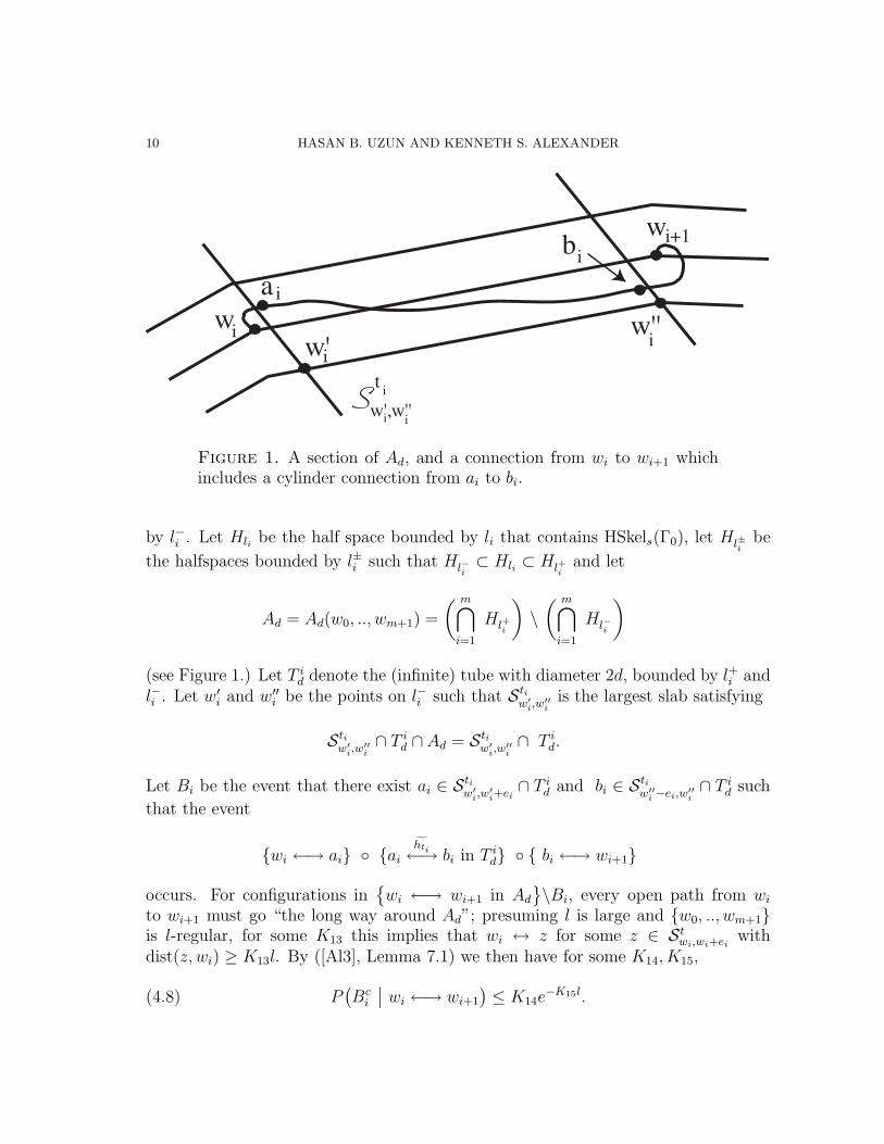
By (4.3) for our chosen s, the deviation between Co(Γ0) and Int(HPaths(Γ0)) insideit does not exceed θl1/3(log l)−2/3. Let li be the line through wi and wi+1. Weset d = 2θl1/3(log l)−2/3, and define Ad, the annular tube of diameter 2d aroundHSkels(Γ0), as follows. Denote the line parallel to li which is d units outside ofHSkels(Γ0) by l+i and the line parallel to li which is d units in the opposite direction

10 HASAN B. UZUN AND KENNETH S. ALEXANDER

w

a

b

w'

w

i

i

i

i

i

i+1

w''

i iw',w''

ti

S

Figure 1. A section of Ad, and a connection from wi to wi+1 whichincludes a cylinder connection from ai to bi.

by l−i . Let Hli be the half space bounded by li that contains HSkels(Γ0), let Hl±ibe

the halfspaces bounded by l±i such that Hl−i⊂ Hli ⊂ Hl+i

and let

Ad = Ad(w0, .., wm+1) =

( m⋂

i=1

Hl+i

)\( m⋂

i=1

Hl−i

)

(see Figure 1.) Let T id denote the (infinite) tube with diameter 2d, bounded by l+i and

l−i . Let w′i and w′′

i be the points on l−i such that Stiw′

i,w′′i

is the largest slab satisfying

Stiw′

i,w′′i∩ T i

d ∩Ad = Stiw′

i,w′′i∩ T i

d.

Let Bi be the event that there exist ai ∈ Stiw′

i,w′i+ei∩ T i

d and bi ∈ Stiw′′

i −ei,w′′i∩ T i

d such

that the event

{wi ←→ ai} ◦ {ai

hti←→ bi in T id} ◦ { bi ←→ wi+1}

occurs. For configurations in{wi ←→ wi+1 in Ad

}\Bi, every open path from wi

to wi+1 must go “the long way around Ad”; presuming l is large and {w0, .., wm+1}is l-regular, for some K13 this implies that wi ↔ z for some z ∈ St

wi,wi+eiwith

dist(z, wi) ≥ K13l. By ([Al3], Lemma 7.1) we then have for some K14, K15,

(4.8) P(Bc

i

∣∣ wi ←→ wi+1

)≤ K14e

−K15l.

LOWER BOUNDS FOR BOUNDARY ROUGHNESS 11

Lemma 4.3. There exists constants K14, K15 > 0 such that for {w0, .., wm+1} l-regular and ǫ, ti as in the preceeding, we have

P (wi ↔ wi+1 in Ad

∣∣wi ↔ wi+1)(4.9)

≤ K14 exp (−K15l) +∑

ai,bi

P (ai ↔ bi in T id

∣∣ ai

hti↔ bi)

where the sum is over all ai ∈ Stiw′

i,w′i+ei∩ T i

d ∩ (Z2)∗ and bi ∈ Stiw′′

i ,w′′i −ei∩ T i

d ∩ (Z2)∗.

Proof. By (4.8) we can bound P (wi ↔ wi+1 in Ad) by

K14e−K15lP (wi ↔ wi+1) +

∑

ai,bi

P({wi ↔ ai} ◦ {ai

hti←→ bi in T id} ◦ {bi ↔ wi+1}

),

where the sum is over all ai ∈ Stiw′

i,w′i+ei∩ T i

d ∩ (Z2)∗ and bi ∈ Stiw′′

i ,w′′i −ei∩ T i

d ∩ (Z2)∗.

We now apply the BK and FKG inequalities:

∑ai,bi

P

({wi ↔ ai} ◦ {ai

hti↔ bi in T id} ◦ {bi ↔ wi+1}

)

≤∑

ai,bi

P (wi ↔ ai) P (ai

hti↔ bi in T id) P (bi ↔ wi+1),

=∑

ai,bi

P (wi ↔ ai) P (ai

hti↔ bi) P (ai

hti↔ bi in T id | ai

hti↔ bi) P (bi ↔ wi+1)

≤∑

ai,bi

P (wi ↔ wi+1) P (ai

hti↔ bi in T id | ai

hti↔ bi),

and (4.9) follows. �

In order to bound the probability of the event{ai

hti←→ bi in T id

}using the renewal

structure of cylinder connectivities, we need control of the size of |bi−ai| to apply (3.1).The parallelogram Sti

w′i+e,w′′

i −e∩T id has 2 short sides (the sides not parallel to wi+1−wi),

one near wi and the other near wi+1 (see Figure 1). It follows easily from the factthat wi+1 − wi, ti are in the wedge V that for every a in the short side near wi wehave |wi − a| ≤ 2d

√2, and analogously for wi+1. Therefore

|wi − ai| ≤ 2d√

2 + 1, |wi+1 − bi| ≤ 2d√

2 + 1,

and hence

(4.10)∣∣(wi+1 − wi)− (bi − ai)

∣∣≤ 4d√

2 + 2.

Since

(4.11) τ(wi+1 − wi) = (ti, wi+1 − wi)2,

12 HASAN B. UZUN AND KENNETH S. ALEXANDER

provided l is large we have

(4.12) (ti, bi − ai)2 ≥ (1− ǫ)τ(bi − ai)

for our chosen ǫ.

Lemma 4.4. Given ǫ, ti, ai, bi as in the preceeding and δ as in (3.1), there existsν ′ > 0 such that provided l is sufficiently large,

P(|Rti

ai,bi| < δ|bi − ai|

∣∣ ai

hti↔ bi

)≤ exp(−ν ′|bi − ai|).(4.13)

Proof. From ([Al3] equation (7.6)), for some K16, K17 > 0, we have

P(ai

hti↔ bi

)≥ K16|bi − ai|−K17 exp

(− τ(bi − ai)

).(4.14)

By (4.12), Lemma 3.3 applies; with (4.14) this shows that for some ν > 0,

P(|Rti

ai,bi| < δ|bi − ai|

∣∣ ai

hti↔ bi

)(4.15)

≤ 1

K16

|bi − ai|K17 exp(− (ti, bi − ai)2 + τ(bi − ai)− ν|bi − ai|

).

By (4.10) and (4.11), we have

− (ti, bi − ai)2 + τ(bi − ai)− ν|bi − ai|≤ 2τ(wi+1 − wi − bi + ai)− ν|bi − ai|≤ K18(4d

√2 + 2)− ν|bi − ai|

for some K18 > 0. Since d is small compared to |bi − ai|, using this bound in (4.15),for some constant ν ′ < ν we have (4.13). �

Next, we will define orthogonal increments between adjacent regeneration points.There is no canonical choice of direction relative to which increments are defined; wewill use the direction orthogonal to the line joining wi and wi+1.

Definition 4.5. For any x ∈ Stiwi,wi+1

, define f : Stiw′

i,w′′i→ R as follows:

f(x) =

{dist(x, li), if x is above the line li, joining wi and wi+1,

− dist(x, li), if x is on or below the line li.

For the following definitions assume ai

hti↔ bi. The regeneration points between ai

and bi have a natural ordering according to their distance from Htiai

.

Definition 4.6. For r′ ∈ Stiai,bi

define ∆ : Stiai,bi→ R as follows:

∆(r′) =

f(r′), if r′ is the first regeneration point,

f(r′)− f(r), if r, r′ are successive regeneration points,

0 if r′ is not a regeneration point.

LOWER BOUNDS FOR BOUNDARY ROUGHNESS 13

Definition 4.7. For Htiz ⊂ Sti

ai,bidefine

∆(Htiz ) =

{∆(r′) if there is a regeneration point r′ ∈ Hti

z ,

0 otherwise.

We will refer to the values ∆(r) as increments. We need to show that, given ai

hti↔ bi,there are unlikely to be too many small increments. This will be proved by showingthat a positive proportion of increments have magnitude greater than equal to 1/2,with high probability. This result will be used to bound the variance of sums ofincrements from below.

For δ as in Lemma 3.3, and ai, bi fixed, let N = ⌊δ|bi − ai|⌋, and R = ⌊N/8⌋. LetU be the collection of all (z1, · · · , zR) such that for j = 1, · · · , R, we have

(i) zj ∈ Stiai,bi

; zj is on the line through wi, parallel to ti,(ii) (ti, z1)2 < (ti, z2)2 < · · · < (ti, zR)2,(iii) (IntSti

zj−4ei,zj+4ei) and (IntSti

zk−4ei,zk+4ei) are disjoint for j 6= k.

By property (i), there is a bijection pairing {z1, z2, · · · , zR} ∈ U and the set of linesHti

zjpassing through the points {z1, z2, · · · , zR}. Suppose Rti

ai,bi= {r1, r2, · · · , rI},

with I ≥ N . Next, we define Qtiai,bi

= {σ1, .., σR} ⊂ Rtiai,bi

according to the followingalgorithm:

(1) σ1 = rk1, where k1 is the smallest integer satisfying (ti, ai + 4ei)2 ≤ (ti, rk1

)2,(2) σj = rkj

, where kj is the smallest integer satisfying (ti, σj−1 +8ei)2 ≤ (ti, rkj)2,

for j = 2, 3, · · · , R.

For j ≥ 2, this algorithm can skip at most 7 regeneration points after σj−1 before itselects σj ; under the assumption that there are at least N regeneration points, it willsuccessfully choose exactly R regeneration points. (Qti

ai,biis undefined when there

are fewer than N regeneration points, so |Qtiai,bi| = R whenever Qti

ai,biis defined.)

Notice that, for some (z1, z2, · · · , zR) ∈ U , the regeneration point σj occurs on Htizj

,

for j = 1, 2, · · · , R. Also, since the slope of ti is rational, the line Htiσj

contains otherlattice points, which are also possible locations for the jth regeneration point, whenonly Hti

σjis specified.

Lemma 4.8. Given ǫ, ti, ai, bi as in the preceeding, for δ > 0 from (3.1), there existγ, ϕ > 0 such that(4.16)

P

( N∑

k=2

δ{|∆(rk)|≥ 1

2} ≤ γ|bi − ai| ; |Rti

ai,bi| > δ|bi − ai|

∣∣∣∣ ai

hti↔ bi

)≤ exp

(− ϕ|bi − ai|

).

14 HASAN B. UZUN AND KENNETH S. ALEXANDER

Proof. For some γ > 0 to be specified later, we write

P

( N∑

k=2

δ{|∆(rk)|≥ 1

2} ≤ γ|bi − ai| ; |Rti

ai,bi| > N

∣∣∣∣ ai

hti↔ bi

)(4.17)

≤∑

(z1,··· ,zR)∈U

P

(Qti

ai,bi⊂

R⋃

j=1

Htizj

;N∑

k=2

δ{|∆(rj)|≥1

2} ≤ γ|bi − ai|

∣∣∣∣ ai

hti↔ bi

)

≤∑

(z1,··· ,zR)∈U

P

(Qti

ai,bi⊂

R⋃

j=1

Htizj

;R∑

j=2

δ{|∆(H

tizj

)|≥ 1

2}≤ γ|bi − ai|

∣∣∣∣ ai

hti↔ bi

)

≤∑

(z1,··· ,zR)∈U

P

(Qti

ai,bi⊂

R⋃

j=1

Htizj

∣∣∣∣ ai

hti↔ bi

)×

P

( R∑

j=2

δ{|∆(H

tizj

)|≥ 1

2}≤ γ|bi − ai|

∣∣∣∣ Qtiai,bi⊂

R⋃

j=1

Htizj

; ai

hti↔ bi

).

We will bound the second probability in the last sum. In order to do this, we

will describe a “renewal shifting” procedure. For ω ∈ {Qtiai,bi⊂ ∪R

j=1Htizj

; ai

hti↔bi}, satisfying |∆(Hti

zj)| < 1

2for some fixed j ≥ 2, this procedure will produce a

configuration ω ∈ {Qtiai,bi⊂ ∪R

j=1Htizj

; ai

hti↔ bi}, which has at most a bounded number

of bonds different from ω, and which satisfies |∆(Htizj

)| ≥ 12. Moreover, this procedure

maps at most 2m configurations to the same ω, where m is the number of possibly-adjusted bonds. Once this procedure is described, for constants c1, c2, · · · , cj−1 weget

P

(|∆(Hti

zj)| < 1/2

∣∣∣∣ Qtiai,bi⊂

R⋃

j=1

Htizj

; ai

hti↔ bi ; ∆(Htizk

) = ck, 1 ≤ k < j

)(4.18)

≤ λ′ P

(|∆(Hti

zj)| ≥ 1/2

∣∣∣∣ Qtiai,bi⊂

R⋃

j=1

Htizj

; ai

hti↔ bi ; ∆(Htizk

) = ck, 1 ≤ k < j

),

where λ′ = λ′(p) > 0. This yields

P

(|∆(Hti

zj)| ≥ 1/2

∣∣∣∣ Qtiai,bi⊂

R⋃

j=1

Htizj

; ai

hti↔ bi; ∆(Htizk

) = ck, for 1 ≤ k < j

)

≥ 1

1 + λ′

LOWER BOUNDS FOR BOUNDARY ROUGHNESS 15

which is sufficient to bound the last probability in (4.17) by P(X < γ|bi−ai|), where

X is binomially distributed with parameters R−1 and p∗ = 11+λ′ . Taking γ < p∗ and

using a bound from [Ho] we have

P(X < γ|bi − ai|

)≤ exp

(−(R− 1)(p∗ − γ)2

2

)≤ exp(−ϕ|bi − ai|

),

for some ϕ > 0. Using this in the right side of (4.17) and observing that the events

{Qtiai,bi⊂ ⋃R

j=1Htizj} are disjoint for distinct (z1, z2, · · · , zR) ∈ U , we obtain (4.16),

after summing over all (z1, z2, · · · , zR) ∈ U .The proof will be completed by description of the “renewal shifting” procedure.

For a given configuration ω ∈ {Qtiai,bi⊂⋃R

j=1Htizj

; ai

hti↔ bi} and a fixed j ≤ R, let

us assume |∆(Htizj

)| < 12, for some j. We will define ω by modifying some dual bonds

inside Stizj−4ei,zj+4ei

. Since ti has slope rq, there exists infinitely many equally spaced

lattice points on the line Htizj

. We will use one of the two lattice points on Htizj

closest

to the regeneration point σj . Call these locations uj and vj, with uj = σj + (−r, q)and vj = σj + (r,−q). The configuration ω has open dual bonds 〈σj − ei, σj〉 and〈σj , σj + ei〉.

There exists a path γLj from σj−2ei to uj−ei in Sti

zj−3ei,zj−eihaving all steps upward

or leftward, with γLj ∩ Hti

σj−ei= {uj − ei}, and similarly a path γR

j from σj + 2ei to

uj +ei in Stizj+ei,zj+3ei

having all steps upward or leftward with γRj ∩Hti

σj+ei= {uj +ei}.

Let Aj be the closed region bounded by γLj , γR

j and the horizontal lines through σj

and uj. To make our choice of γLj , γR

j unique, let us specify that Aj be maximal under

the constraints we have imposed on γLj , γR

j . Let Dj be the set of all dual bonds havingone endpoint in ∂Aj and the other outside Aj. Note there are at most 12q dual bondscontained in Aj , and at most 2r + 2q + 10 dual bonds in Dj. Let ω be such that

(1) all dual bonds in ∂Aj\{〈σj − ei, σj〉, 〈σj , σj + ei〉} are open;(2) all other dual bonds contained in Aj are closed;(3) all dual bonds in Dj ∩C

tiai,bi

(ω) are open;

(4) all dual bonds in Dj\Ctiai,bi

(ω) are closed;(5) all other dual bonds retain their state from ω.

In the altered configuration ω, the regeneration point is still on Htizj

but shifted from

σj to uj. After these alterations, if |∆(Htizj

)| ≥ 12, then we are done. It is possible that

|∆(Htizj

)| < 12, for the following reason. Let k be such that zj = rk. If there are other

regeneration points in Stizj−3ei,zj+3ei

in ω, shifting the regeneration point to uj will de-

stroy these regeneration points; any regeneration points in Stizj−4ei,zj+4ei

\Stizj−3ei,zj+3ei

in ω may or may not be destroyed, depending on the exact geometry of the situation.At any rate, if rk−1 is destroyed, the new “preceding regeneration point” for zj will be

outside the slab Stizj−3ei,zj+3ei

, equal to rk−2 or rk−3, and we may have |∆(Htizj

)| < 12

in

16 HASAN B. UZUN AND KENNETH S. ALEXANDER

ω, depending on the location of this new preceding regeneration point relative to li. Ifthis is the case we shift the regeneration point from σj to vj instead of uj. For this weuse paths γL

j from σj−2ei to vj−ei and γRj from σj +2ei to vj + ei in place of γL

j and

γRj , under an analogous maximality constraint. Let xL

j (respectively xRj ) be the site in

γLj (respectively γR

j ) closest to Htiσj−3ei

(respectively Htiσj+3ei

). Due to the maximality

constraints we have imposed, since all our slabs have boundaries with slope −q/r,xL

j + (r,−q) is the site in γLj closest to Hti

σj−3ei, and xR

j + (r,−q) is the site in γRj

closest to Htiσj+3ei

. This means that γLj and γL

j intersect the same slabs orthogonal

to ti, and similarly for γRj and γR

j . As a consequence, the same regeneration pointsare destroyed, regardless of whether we shift to uj or vj, so ω has the same preceding

regeneration point either way. It follows that if shifting to uj results in |∆(Htizj

)| < 12,

then shifting to vj results in |∆(Htizj

)| ≥ 12, i.e. there is always a shift (the one we

choose to create ω) which results in |∆(Htizj

)| ≥ 12.

Note that only a bounded number of different configurations may map to the sameconfiguration ω. In any case, ω and ω yield the same value of Qti

ai,bi, and the proba-

bilities of ω and ω are within a bounded factor (depending on p), which yields (4.18),completing the proof. �

5. Exchangeability of Increments

The core idea in our proof of (2.1) is to make use of the renewal structure ofconnectivities, for connections between any two consecutive extreme points wi, wi+1

in the s-hull skeleton with i ∈ L, to see that the increments ∆(rj), 2 ≤ j ≤ N , forman exchangeable sequence under certain conditioning, that is, the joint distribution ispermutation invariant. The partial sums of this sequence behave like those of an i.i.d.sequence, and from this we can show that with high probability, the path of opendual bonds will not stay in the “narrow tube” from wi to wi+1 with diameter 2d =4θl1/3(log l)−2/3. In this section we will prove this exchangeability. Let ǫ, ti, ai, bi be asin the preceeding, δ as in (3.1) and γ as in (4.16). Define the event E = E(ai, bi, ti, γ, δ)by

E =

{ai

hti←→ bi

}∩{|Rti

ai,bi| ≥ δ|bi − ai|

}∩{ N∑

k=2

δ{|∆(rk)|≥ 1

2} ≥ γ|bi − ai|

}.

For v, w ∈ T id ∩ Sti

ai,bi∩ (Z2)∗, define the sets

V (v, w) =

{ζ = (ζ2, ..., ζN) ∈ RN−1 : |ζ2| ≥ |ζ3| ≥ · · · ≥ |ζN | ;

N∑

k=2

ζi = f(w)− f(v)

}.

For given ζ ′ ∈ V (v, w), let F = F (v, w, ζ ′) denote the event that the following allhold:

LOWER BOUNDS FOR BOUNDARY ROUGHNESS 17

(i) ai

hti←→ bi ,(ii) the first and N -th regeneration points are at v and w, respectively,(iii) for some permutation π : {2, · · · , N} → {2, · · · , N}, we have

∆(r2) = ζ ′π(2), ∆(r3) = ζ ′

π(3), · · · , ∆(rN) = ζ ′π(N).

Observe that condition (iii) determines the values of the ∆(rk)’s up to an ordering,

and (ii) and (iii) imply∑N

k=2 ∆(rk) = f(w)− f(v).

Lemma 5.1. For fixed ai, bi, ti, γ, δ, v, w, ζ ′, E, F as in the preceding, ∆(r2), · · · , ∆(rN)are exchangeable under the measure P (· | E ∩ F ).

Proof. E ∩ F determines the location of first and N -th regeneration points, andvalues of increments in between them, up to an ordering. We will first show how toexchange any two adjacent increments. Consider a configuration ω ∈ E ∩ F , with∆(r2) = ζ ′

2, ∆(r3) = ζ ′3, · · · , ∆(rN) = ζ ′

N . For fixed k ≥ 2, let us consider increments∆(rk) and ∆(rk+1). By definition of regeneration points, the bonds that are onlypartially in the slab Sti

rk,rk+1or have exactly one endpoint in the within-slab cluster

containing rk and rk+1 are all vacant. We construct a configuration ω such that outsideSti

rk−1,rk+1we have ω = ω. We obtain ω by interchanging the relative positions of the

configurations ωS

tirk−1,rk

and ωS

tirk,rk+1

and moving the bonds crossing Htirk

so that they

cross Htirk−1+(rk+1−rk) instead. The latter move is done in such a way that the relative

positions of the bonds remain the same, with the old position relative to rk becomingthe new position relative to rk−1 + (rk+1 − rk). More precisely, the configurationin Sti

rk−1,rkis translated by rk − rk−1, the configuration in Sti

rk,rk+1is translated by

rk−rk+1, and each bond touching or crossing Htirk

is translated by rk−1 +(rk+1−2rk).This moves the k-th regeneration point from rk to rk−1 +(rk+1− rk), without alteringthe locations of other regeneration points. The configuration ω is in E ∩ F and theincrements of ω satisfy

∆(rk) = ζ ′j+1, ∆(rk+1) = ζ ′

j, and ∆(rm) = ζ ′m, for 2 ≤ m ≤ N, k 6= m, m + 1.

Moreover, replacing ω with ω does not affect probability under the measure P (·| E ∩F ), due to shift invariance. We can repeat the exchanging of adjacent incrementsuntil we achieve the desired permutation of {2, 3 · · · , N}, and the lemma follows. �

6. Staying in the Narrow Tube

In this section, we will show that there is an extra probabilistic cost associated tothe event that Γ0 stays in the narrow tube T i

d, between ai and bi . The proof involvesrandomization of the order of the increments, using exchangeability.

Lemma 6.1. Let i ∈ L and let ǫ, ti, ai, bi be as in the preceeding. Let δ be as in (3.1)and γ as in (4.16). There exists κ = κ(γ) > 0 such that for all v, w ∈ T i

d∩Stiai,bi∩(Z2)∗

18 HASAN B. UZUN AND KENNETH S. ALEXANDER

and ζ ′ ∈ V (v, w)∩ [−2d, 2d]N , for E = E(ai, bi, ti, γ, δ), F = F (v, w, ζ ′), provided l islarge we have

P

(ai

hti←→ bi in T id

∣∣∣∣ E ∩ F

)≤ 2 exp

(−κ|wi+1 − wi|d2

).(6.1)

Proof. Observe that when ai

hti←→ bi in T id, every open path from ai to bi in T i

d mustpass through all regeneration points. Thus

(6.2) P(ai

hti←→ bi in T id | E ∩ F

)≤ P ({r1, r2, · · · , rN} ⊂ T i

d ∩ Stiai,bi

∣∣ E ∩ F).

We can relate the last probability to an event involving increments. If 1 ≤ k1 < k2 ≤N and

∣∣∑k2−1j=k1

∆(rj+1)∣∣ > 2d, then the k1-th or k2-th regeneration point must lie

outside of T id. Therefore,

P ({r1, r2, · · · , rN+1} ∈ T id ∩ Sti

ai,bi

∣∣ E ∩ F)

≤ P

(∣∣∣∣k2−1∑

j=k1

∆(rj+1)

∣∣∣∣ ≤ 2d, for all 1 ≤ k1 < k2 ≤ N

∣∣∣∣ E ∩ F

).(6.3)

Instead of looking at partial sums for all possible values of k1, k2, we will considerdisjoint blocks of increments with random lengths X1, X2, · · · , XB satisfying X1 +· · ·+XB < N , for some B ∈ N. Let Sn =

∑nk=1 Xk, for n = 1, · · · , B, and let S0 = 0.

Then (6.3) is bounded by

P

( B⋂

k=1

{max

1≤m≤Xk

∣∣∣∣Sk−1+m∑

j=Sk−1+1

∆(rj+1)

∣∣∣∣ ≤ 2d

}∣∣∣∣ E ∩ F

),(6.4)

where we define X0 = 0. If we take Xk, for 1 ≤ k ≤ B, to be deterministic, theincrements on these disjoint blocks will not be independent of the increments onother blocks. In order to reduce the dependence between these disjoint blocks, wewill take the Xk’s to be (non-independent) binomially distributed random variables.Next, we use exchangeability of increments to write (6.4) in an equivalent form. Forbinomially distributed X1 with parameters, N − 1 and p0, with p0 to be specifiedlater,

X1+1∑

j=2

∆(rj)d=

N∑

j=2

δj1ζ′j

where the δj1, j = 2, .., N are i.i.d. Bernoulli random variables with parameter p0.That is, the sum of first X1 increments have the same distribution as the sum ofincrements randomly selected according to the δj1’s. Continuing this way, for eachfollowing random block, we replace the sum of increments corresponding to that blockwith a sum of increments that are randomly selected from those increments remaining

LOWER BOUNDS FOR BOUNDARY ROUGHNESS 19

after the earlier steps of the increment–selection process. More precisely, we do thefollowing. Define p0 and the number of blocks by

p0 =K19d

2

|wi+1 − wi|, B = ⌊ 1

2p0

⌋,

where K19 = K19(γ) is sufficiently large constant, to be specified later. Observe thatp0 = O((log l)−1). For all 2 ≤ j ≤ N , define

δjk =

{0 with probability pk = 1−kp0

1−(k−1)p0

1 with probability 1− pk = p0

1−(k−1)p0,

(6.5)

with {δjk, j = 2, · · ·N , k = 1, · · · , B} independent random variables. Also defineYjk = (1− δj1)(1− δj2) · · · (1− δjk), for j = 2, .., N , k = 1, .., B. Then we have

Yjk =

{0 with probability kp0

1 with probability 1− kp0

(6.6)

The random variable Yjk = 1 says that the j-th increment is not selected for the firstk blocks, and Yj(k−1)δjk = 1 says that the j-th increment is selected for the k-th block.We define the length of the k-th block Xk as

Xk =N∑

j=2

Yj(k−1)δjk, for k = 1, 2, · · · , B.

It can be easily seen from (6.5) and (6.6) that the Xk’s are binomially distributed(but not independent) with parameters N − 1 and p0. By exchangeability, we canrewrite (6.4) as

P

( B⋂

k=1

{max

2≤m≤N

∣∣∣∣m∑

j=2

Yj(k−1)δjkζj

∣∣∣∣ ≤ 2d

} ∣∣∣∣ E ∩ F

),(6.7)

since∑B

k=1 Xk ≤ N , which holds because no j can be chosen for more than one block.We let

Dk =

{ω : max

2≤m≤N

∣∣∣∣m∑

j=2

Yj(k−1)δjkζj

∣∣∣∣ ≤ 2d

}.

We need to control the number of increments |ζj| ≥ 1/2 which remain after someblocks have been selected. By definition of E, there are at least ⌊γ|bi − ai|⌋ such

increments before the first block is selected. Let g =√

B⌊γ|bi − ai|⌋, let G1 = E∩F ,and for k = 2, · · · , B define

Gk =

{ω :

∣∣∣∣( ⌊γ|bi−ai|⌋∑

j=2

Yj(k−1)

)− (1− (k − 1)p0)⌊γ|bi − ai|⌋

∣∣∣∣ ≤ g

}.

20 HASAN B. UZUN AND KENNETH S. ALEXANDER

Let Ik = {j : Yj(k−1) = 1, 1 ≤ j ≤ N − 1}, be the random set of remaining increment

indices before the k-th block is selected. Then Gk−1 provides control over∣∣Ik ∩

{1, 2, · · · , ⌊γ|bi − ai|⌋}∣∣, the number of remaining increments that are greater than

or equal to 1/2; here we use the monotonicity of the |ζj|’s, and the fact that at least⌊γ|bi − ai|⌋ increments are greater than or equal to 1/2. By (6.2)–(6.4) we have

P(ai

hti←→ bi in T id

∣∣ E ∩ F)

≤ P

( B⋂

k=1

(Dk ∩Gk

) ∣∣∣∣ E ∩ F

)+ P

([ B⋂

k=1

Gk

]c ∣∣∣∣ E ∩ F

)(6.8)

First we bound the probability in (6.8) of a large deviation for some block for thenumber of available large increments, using a bound from [Ho]:

P

([ B⋂

k=1

Gk

]c ∣∣∣∣ E ∩ F

)≤

B∑

k=2

P (Gck | E ∩ F )(6.9)

≤ 2B exp( −2g2

⌊γ|bi − ai|⌋)

= 2B exp(−2B)

≤ exp(−B),

where the last inequality holds for l sufficiently large. Next, we consider the prob-ability the probability of staying in the narrow tube in the absence of such a largedeviation. This probability from (6.8) can be written

P(D1

∣∣ E ∩ F)×

B∏

k=2

P

(Dk ∩Gk

∣∣∣∣ E ∩ F ∩k−1⋂

j=1

(Dj ∩Gj)

)(6.10)

≤ P(D1

∣∣ E ∩ F)×

B∏

k=2

P

(Dk

∣∣∣∣ E ∩ F ∩k−1⋂

j=1

(Dj ∩Gj)

).

We will conclude by showing

P

(Dk

∣∣∣∣ E ∩ F ∩k−1⋂

j=1

(Dj ∩Gj)

)≤ 2/3,(6.11)

for k ≥ 2. The proof that P(D1

∣∣ E ∩F)≤ 2/3 follows by the same technique. Let

us fix k ≥ 2. We define a family of sets of indices:

Ik =

{Υ ⊂ {2, · · · , N − 1} :

∣∣∣∣⌊γ|bi−ai|⌋∑

j=2

δ{j∈Υ} − (1− (k − 1)p0)⌊γ|bi − ai|⌋∣∣∣∣ ≤ g

}.

LOWER BOUNDS FOR BOUNDARY ROUGHNESS 21

For Υ ∈ Ik, and n ≤ N − 1, define

Υn = Υ ∩ {2, 3, · · · , n}Observe that if Gk−1 occurs then Ik ∈ Ik. It follows that

P

(Dk

∣∣∣∣ E ∩ F ∩k−1⋂

j=1

(Dj ∩Gj)

)

=∑

Υ∈Ik

P

(Dk ∩ {Ik = Υ}

∣∣∣∣ E ∩ F ∩k−1⋂

j=1

(Dj ∩Gj)

).(6.12)

Fix Υ ∈ Ik and define the event Hk = [Ik = Υ] ∩E ∩ F ∩⋂k−1

j=1(Dj ∩Gj). Define

Q(k, Υn) =

[1

2

(p0(1− kp0)

(1− (k − 1)p0)2

)∑

j∈Υn

(ζ ′j)

2

]1/2

,

so that

Var

( ∑

j∈Υn

δjkζ′j

∣∣∣∣ Hk

)= 2[Q(k, Υn)]

2.

For any index set Υ ∈ Ik, one of three possibilities has to hold:

(1) for all n = 2, 3, ..., N∣∣∣∣E( ∑

j∈Υn

δjkζ′j

∣∣∣∣ Hk

)∣∣∣∣ =

∣∣∣∣∑

j∈Υn

p0

1− (k − 1)p0ζ ′j

∣∣∣∣ ≤ 2d + Q(k, Υn);

(2) for some n0, 2 ≤ n0 ≤ N

E

( ∑

j∈Υn0

δjkζ′j

∣∣∣∣ Hk

)> 2d + Q(k, Υn0

);

(3) for some n0, 2 ≤ n0 ≤ N

−E

( ∑

j∈Υn0

δjkζ′j

∣∣∣∣ Hk

)> 2d + Q(k, Υn0

).

In case (2),

P(Dk

∣∣ Hk

)

≤ P

(− 2d ≤

∑

j∈Υn0

δjkζ′j ≤ 2d

∣∣∣∣ Hk

)

≤ P

( ∑

j∈Υn0

[δjkζ

′j −

p0

1− (k − 1)p0ζ ′j

]< −Q(k, Υn0

)

∣∣∣∣ Hk

)

22 HASAN B. UZUN AND KENNETH S. ALEXANDER

By Chebyshev’s inequality, the last probability is bounded by

1

1 +[Q(k,Υn0

)]2

2[Q(k,Υn0)]2

=2

3.

In case (3), similarly, P (Dk | Hk) ≤ 2/3. Case (1) requires some extra work. UsingKolmogorov’s inequality we get

P (Dk | Hk) ≤ P

(max

2≤m≤N

∣∣∣∑

j∈Υm

δjkζ′j −

p0

1− (k − 1)p0ζ ′j

∣∣∣ < 4d + Q(k, ΥN)

∣∣∣∣ Hk

)

≤[6d + Q(k, ΥN)

]2

2[Q(k, ΥN)]2.

The proof of (6.11) will be concluded by showing

d2

2[Q(k, ΥN)]2≤ 1

98,

since this implies

[6d + Q(k, ΥN)

]2

2[Q(k, ΥN)]2≤ 2/3.

Since Υ ∈ Ik we have

∑

j∈Υ

(ζ ′j)

2 ≥ 1

4

∑

j∈Υ

δ{|ζ′j |≥1/2

}

≥ 1

4|Υ⌊γ|bi−ai|⌋|

≥ 1

4

((1− (k − 1)p0)⌊γ|bi − ai|⌋ − g

)

≥ 1

8

(⌊γ|bi − ai|⌋ − 2g

)

≥ 1

16γ|bi − ai|

since 12≤ 1− kp0 ≤ 1, for sufficiently large l. Therefore,

d2

2[Q(k, N)]2≤ 16d2((1− (k − 1)p0)

2)

p0(1− kp0)γ|bi − ai|≤ 32d2

p0γ|bi − ai|=

32|wi+1 − wi|K19γ|bi − ai|

By (4.10), we can choose K19 = K19(γ) (from the definition of p0) sufficiently largeso that the last expression is less than 1/98, for large l. Under each case (1)-(3) we

LOWER BOUNDS FOR BOUNDARY ROUGHNESS 23

have shown P (Dk | Hk) ≤ 2/3, for arbitrary Υ ∈ Ik. With (6.12) this proves (6.11).Using (6.8)–(6.10) we get

P(ai

hti←→ bi in T id

∣∣ E ∩ F)≤ (2/3)B + e−B

≤ 2 exp(−κ|wi+1 − wi|

d2

),

for some κ > 0, which concludes the proof of the lemma. �

Lemma 6.2. Let ǫ, ti, ai, bi be as in the preceeding, with i ∈ L. Let δ be as in (3.1),γ as in (4.16) and κ as in (6.1). Provided l is sufficiently large we have

P

(ai

hti←→ bi in T id

∣∣ ai

hti←→ bi

)≤ 3 exp

(−κ|wi+1 − wi|d2

).(6.13)

Proof. Let ν ′ be as in (4.13) and ϕ as in (4.16). We will consider intersections of the

event {ai

hti←→ bi in T id} with the events E = E(ai, bi, ti, δ, γ) and Ec, separately. First

we have

P

(Ec | ai

hti←→ bi

)

≤ P

(|Rti

ai,bi| < δ|bi − ai|

∣∣ ai

hti←→ bi

)

+P

( N∑

j=1

δ{|∆(rj)|≥1

2} ≤ γ|bi − ai| ; |Rti

ai,bi| > δ|bi − ai|

∣∣∣∣ ai

hti↔ bi

)

≤ exp(−ν ′|bi − ai|) + exp(−ϕ|bi − ai|),(6.14)

by (4.13) and (4.16). Since i ∈ L, this bound is small compared to the right sideof (6.13). Next, we have

P

({ai

hti←→ bi in T id} ∩ E

∣∣ ai

hti←→ bi

)(6.15)

≤∑

v,w∈T id∩S

tiai+3ei,bi

∩(Z2)∗

[ ∑

ζ′∈V (v,w)

P

({ai

hti↔ bi in T id} ∩ E ∩ F (v, w, ζ ′)

∣∣ ai

hti↔ bi

)],

where the first sum is over all possible locations of first and N-th regeneration points,and the second sum is over all possible sets of increments between v and w. If themagnitude of one of these increments is greater than 2d, this implies at least oneregeneration point must be outside the tube T i

d. Therefore, we can restrict the second

24 HASAN B. UZUN AND KENNETH S. ALEXANDER

sum to ζ ′ ∈ V (v, w) ∩ [−2d, 2d]N , and the last sum is bounded by(6.16)

∑

v,w∈T id∩S

tiai+3ei,bi

∩(Z2)∗

[ ∑

ζ′∈V ∩[−2d,2d]N

P

({ai

hti↔ bi in T id} ∩ E ∩ F (v, w, ζ ′)

∣∣ ai

hti↔ bi

)].

For the remainder of the proof, our sums are over v, w ∈ T id ∩ Sti

ai+3ei,bi∩ (Z2)∗ and

ζ ′ ∈ V (v, w) ∩ [−2d, 2d]N . We can write the last expression as

∑

v,w

[∑

ζ′

P(E ∩ F (v, w, ζ ′)| ai

hti↔ bi

)P(ai

hti↔ bi in T id

∣∣ E ∩ F (v, w, ζ ′))]

≤ 2 exp

(−κ|wi+1 − wi|d2

)∑

v,w

∑

ζ′

P(E ∩ F (v, w, ζ ′)| ai

hti↔ bi

),

using (6.1). Taking the double sum over the probabilities of disjoint events, in viewof (6.15) and (6.16) we get

P

({ai

hti←→ bi in T id} ∩ E

∣∣ ai

hti←→ bi

)≤ 2 exp

(−κ|wi+1 − wi|d2

).

Combining this with (6.14) completes the proof. �

7. Assembling the Segments

In the last section, we proved that on every long facet of the ∂HSkels(Γ0), thereis an extra probabilistic cost for staying in the narrow tube. In this section, we willbring the pieces in the preceding sections together to deduce that, there is an extraprobabilistic cost of staying in the annular region Ad (with diameter 2d), throughoutthe boundary of the HSkels(Γ0). We will show that in light of the inequality (4.3),leaving the annular region Ad implies that MLR(Γ0) > θl1/3(log l)−2/3. Then bybounding the number of possible skeletons, we will prove (2.1).

Lemma 7.1. There exists K20 = K20(δ, γ) such that for sufficiently large l, for alll-regular s-hull skeletons {w0, .., wm+1},(7.1)

P({

w0 ↔ w1

}◦ · · · ◦

{wm ↔ wm+1

}in Ad

)≤ exp(−W1l −

K20

θ2l1/3(log l)4/3).

Proof. Using the BK-inequality, we have

P({

w0 ↔ w1

}◦ · · · ◦

{wm ↔ wm+1

}in Ad

)≤

m∏

i=0

P (wi ↔ wi+1 in Ad).(7.2)

This last product can be written as products over long and short sides separately.We will bound the product over long sides further. As before for i ∈ L, let ai ∈

LOWER BOUNDS FOR BOUNDARY ROUGHNESS 25

Stiw′

i,w′i+ei∩ T i

d and bi ∈ Stiw′′

i ,w′′i −ei∩ T i

d; note there are at most 2d choices each for ai

and bi. Using (4.9), (6.13) and l-regularity we have∏

i∈L

P (wi ↔ wi+1 in Ad)(7.3)

≤∏

i∈L

P (wi ↔ wi+1)

[K14 exp (−K15l) + 4d2 max

ai,bi

P (ai ↔ bi in T id

∣∣ ai

hti↔ bi)

]

≤∏

i∈L

P (wi ↔ wi+1)

[K14 exp (−K15l) + 12d2 exp

(−κ|wi+1 − wi|d2

)]

≤∏

i∈L

P (wi ↔ wi+1)

[13d2 exp

(−κ|wi+1 − wi|d2

)].

Now we place a condition on the as-yet-unspecified constant θ; recall that

s =

(θ√

π

2K7

)1/2

l2/3(log l)−1/3, d = 2θl1/3(log l)−2/3.

For some β = β(K5, K7, κ), provided θ is sufficiently small we have

13d2 exp

(−κ|wi+1 − wi|2d2

)≤ 20θ2l2/3(log l)−4/3 exp(−βθ−3/2 log l) ≤ 1,

so that

13d2 exp

(−κ|wi+1 − wi|d2

)≤ exp

(−κ|wi+1 − wi|2d2

).

Therefore, using Lemma 4.2, the right side of (7.3) is bounded by

exp

(− κ

2d2·∑

i∈L

|wi+1 − wi|)·∏

i∈L

P (wi ↔ wi+1)

≤ exp

(− κ√

π

8θ2√

2l1/3(log l)4/3

)·∏

i∈L

P (wi ↔ wi+1).

Using (7.3) and (2.6) we then obtain

m∏

i=0

P (wi ↔ wi+1 in Ad) ≤ exp

(− κ√

π

8θ2√

2l1/3(log l)4/3

) m∏

i=0

P (wi ↔ wi+1)

≤ exp

(− κ√

π

8θ2√

2l1/3(log l)4/3 −

m∑

i=0

τ(wi+1 − wi)

).(7.4)

By l-regularity there exists a dual circuit γ0 with | Int(γ0)| ≥ l2, diam(γ0) ≤ 8√

2 land HSkels(γ0) = {w0, .., wm+1}. The first condition implies diam(γ0) ≥ l, and by

26 HASAN B. UZUN AND KENNETH S. ALEXANDER

definition of W1 we have W(∂Co(γ0) ≥ W1l. Therefore by (4.4), for some K21,

m∑

i=0

τ(wi+1 − wi) ≥ W1l −K21θl1/3(log l)−2/3.

The lemma now follows from this together with (7.2) and (7.4). �

Proof of Theorem 2.1: By (4.6),

P(

MLR(Γ0) ≤ θl1/3(log l)−2/3∣∣ | Int(Γ0)| ≥ l2

)

≤ P({MLR(Γ0) ≤ θl1/3(log l)−2/3} ∩ {diam(Γ0) ≤ 8

√2l}

∣∣ | Int(Γ0)| ≥ l2)

(7.5)

+ exp(−W1l/2).

This means we need only consider l-regular skeletons {w0, · · · , wm+1} for Γ0. When| Int(Γ0)| ≥ l2 we have diam(Γ0) ≥ l and therefore

K7s2

diam(Γ0)< d.

Presuming HSkels(Γ0) = {w0, · · · , wm+1}, this implies ∂Co(Γ0) ⊂ Ad. This meansthat in order to have MLR(Γ0) ≤ θl1/3(log l)−2/3, Γ0 must be entirely inside Ad. Thus

P({MLR(Γ0) ≤ θl1/3(log l)−2/3} ∩ {diam(Γ0) ≤ 8

√2l} ∩ {| Int(Γ0)| ≥ l2}

)

≤∑

{w0,··· ,wm+1}

P

( {HSkels(Γ0) = {w0, · · · , wm}

}

∩{ {

w0 ↔ w1

}◦ · · · ◦

{wm ↔ wm+1

}in Ad(w0, .., wm+1

}}), )(7.6)

where the sum is over all l-regular skeletons. By (4.1) the number of l-regular skeletonsis at most

(K22l2)K23θ−1/2l1/3(log l)1/3 ≤ exp(K24θ

−1/2l1/3(log l)4/3),

for some K22, K23, K24. This together with (7.1) and (7.6) gives

P({MLR(Γ0) ≤ θl1/3(log l)−2/3} ∩ {diam(Γ0) ≤ 8

√2l} ∩ {| Int(Γ0)| ≥ l2}

)

≤ exp

(−W1l −

(K20

θ2− K24

θ1/2

)l1/3(log l)4/3

)

which with (4.5) and (7.5) yields

P(

MLR(Γ0) ≤ θl1/3(log l)−2/3∣∣ | Int(Γ0)| ≥ l2

)

≤ exp

(−(

K20

θ2− K24

θ1/2

)l1/3(log l)4/3 + K11l

1/3(log l)2/3

)+ exp

(− W1l

2

).

For θ > 0, sufficiently small, the last bound tends to 0, as l →∞. �

LOWER BOUNDS FOR BOUNDARY ROUGHNESS 27

References

[Al1] Alexander, K.S., Approximation of subadditive functions and rates of convergence in limiting

shape results, Ann. Probab. 25 (1997), 30–55.[Al2] Alexander, K.S., Power-law corrections to exponential decay of connectivities and correlations

in lattice models, Ann. Probab. 29 (2001), 92–122.[Al3] Alexander, K.S., Cube-root boundary fluctuations for droplets in random cluster models, Com-

mun. Math Phys. 224 (2001), 733–781.[ACC] Alexander K.S., Chayes, J.T., and Chayes L., The Wulff construction and asymptotics of

the finite cluster distribution for two dimensional Bernoulli percolation, Commun. Math. Phys.131 (1990), 1-50.

[BDJ] Baik, J., Deift, P. and Johansson K., On the distribution of the length of the longest increasing

subsequence of random permutations, J. Amer. Math. Soc. 12 (1999), 1119–1178.[CI] Campanino, M. and Ioffe D., Ornstein-Zernike Theory for the Bernoulli bond percolation on

Zd, Ann. Probab. 30 (2002), 652–682.[DH] Dobrushin, R.L. and Hryniv, O., Fluctuations of the phase boundary in the 2D Ising ferro-

magnet, Commun. Math. Phys. 189 (1997), 395–445.[DKS] Dobrushin, R.L., Kotecky, R. and Shlosman, S., Wulff construction. A global shape from local

interaction, Translations of Mathematical Monographs, 104, American Mathematical Society,Providence (1992).

[ES] Edwards, R.G. and Sokal, A.D., Generalization of the Fortuin-Kasteleyn-Swendsen-Wang rep-

resentation and Monte Carlo algorithm, Phys. Rev. D 38 (1988), 2009-2012.[FK] Fortuin, C.M. and Kasteleyn, P.W., On the random cluster model. I. Introduction and relation

to other models, Physica 57 (1972), 536-564.[FKG] Fortuin, C.M., Kasteleyn, P.W. and Ginibre, J., Correlation inequalities on some partially

ordered sets, Commun. Math. Phys. 22 (1971), 89–103.[Ha] Harris T.E., A lower bound for the critical probability in a certain percolation process, Proc.

Camb. Phil. Soc. 56 (1960), 13–20.[Ho] Hoeffding, W., Probability inequalities for sums of bounded random variables, J. Amer. Statist.

Assoc. 58 (1953), 13–30.[Hr] Hryniv, O., On local behaviour of the phase separation line in the 2D Ising model, Probab.

Theory Rel. Fields 110 (1998), 91-107.[IS] Ioffe, D. and Schonmann, R.H., Dobrushin-Kotecky-Shlosman theorem up to the critical tem-

perature, Commun. Math Phys. 199 (1998), 91–107.[Jo] Johansson, K., Discrete orthogonal polynomial ensembles and the Plancherel measure, Ann.

Math. (2) 153 (2001), 259–296.[KPZ] Kardar, M., Parisi, G. and Zhang, Y.-C., Dynamic scaling of growing interfaces, Phys. Rev.

Lett. 56 (1986), 889–892.[Ke] Kesten, H., The critical probability of bond percolation on the square lattice equals 1

2, Commun.

Math. Phys. 74 (1980), 41–59.[KS] Krug, J. and Spohn, H., Kinetic roughening of growing interfaces, in Solids Far from Equi-

librium: Growth, Morphology and Defects (C. Godreche, ed.) 479–582, Cambridge UniversityPress, Cambridge (1991).

[LNP] Licea, C., Newman, C.M. and Piza, M.S.T., Superdiffusivity in first-passage percolation,Probab. Theory Rel. Fields 106 (1996), 559–591.

[Me] Menshikov, M.V., Coindidence of critical points in percolation problems, Soviet Math. Dokl.33 (1986), 856–859.

28 HASAN B. UZUN AND KENNETH S. ALEXANDER

[MS1] Minlos, R.A. and Sinai Ya.G.,The phenomenon of “phase separation” at low temperatures in

some lattice models of a gas. I., Mat. Sb. 73 (1967), 375–448. [English transl., Math. USSR-Sb.2 (1967), 335–395.]

[MS2] Minlos, R.A. and Sinai Ya.G., The phenomenon of ”phase separation” at low temperatures

in some lattice models of a gas. II., Tr. Moskov. Mat. Obshch. 19 (1968), 113–178. [Englishtransl., Trans. Moscow Math Soc. 19 (1968), 121–196.]

[NP] Newman, C.M. and Piza, M.S.T., Divergence of shape fluctuations in two dimensions, Ann.Probab. 23 (1995), 977–1005.

[Pi] Piza, M.S.T., Directed polymers in a random environment: Some results on fluctuations, J.Statist. Phys. 89 (1997), 581–603.

[Ta1] Taylor, J.E., Existence and structure of solutions to a class of nonelliptic variational problems,Symp. Math. 14 (1974), 499-508.

[Ta2] Taylor, J.E., Unique structure of solutions to a class of nonelliptic variational problems, Proc.Sympos. Pure Math. 27 (1975), 419–427.

[Uz] Uzun, H.B., On maximum local roughness of random droplets in two dimensions, Ph.D. disser-tation, Univ. of Southern California (2001).

[vdBK] van den Berg, J. and Kesten, H., Inequalities with applications to percolation and reliability,Journal of Applied Probability 22 (1985), 556–569.

[Wu] Wulff, G., Zur Frage der Geschwingkeit des Wachstums und der Auflosung der Krystallflachen,Z. Kryst. 34 (1901), 449-530.

ALEKS Corporation, 400 N. Tustin Avenue, Suite 300, Santa Ana, CA 92705 USA

E-mail address : huzun@aleks.com

Department of Mathematics DRB 155, University of Southern California, Los

Angeles, CA 90089-1113 USA

E-mail address : alexandr@math.usc.edu