Numerical investigation of the evaporation of two-component droplets

Fuel 90 (2011) 1492–1507

Contents lists available at ScienceDirect

Fuel

journal homepage: www.elsevier .com/locate / fuel

Numerical investigation of the evaporation of two-component droplets

George Strotos a,1, Manolis Gavaises b,⇑, Andreas Theodorakakos c, George Bergeles a

a National Technical University of Athens, Department of Mechanical Engineering 5 Heroon Polytechniou, 15710 Zografos, Athens, Greeceb City University London, School of Engineering and Mathematical Sciences Northampton Square, EC1V 0HB, London, UKc Fluid Research Co. 49 Laskareos Str, 11472, Athens, Greece

a r t i c l e i n f o

Article history:Received 15 June 2010Received in revised form 10 January 2011Accepted 11 January 2011Available online 25 January 2011

Keywords:Droplet evaporationMulti-component evaporationVOFSuspended droplet

0016-2361/$ - see front matter � 2011 Elsevier Ltd Adoi:10.1016/j.fuel.2011.01.017

⇑ Corresponding author.E-mail address: [email protected] (M. Gavaise

1 Present address: Technological Education InstiEngineering Department, Fluid Mechanics LaboratoryAegaleo, 12244, Greece

a b s t r a c t

A numerical model for the complete thermo-fluid-dynamic and phase-change transport processes of two-component hydrocarbon liquid droplets consisting of n-heptane, n-decane and mixture of the two invarious compositions is presented and validated against experimental data. The Navier–Stokes equationsare solved numerically together with the VOF methodology for tracking the droplet interface, using anadaptive local grid refinement technique. The energy and concentration equations inside the liquidand the gaseous phases for both liquid species and their vapor components are additionally solved, cou-pled together with a model predicting the local vaporization rate at the cells forming the interfacebetween the liquid and the surrounding gas. The model is validated against experimental data availablefor droplets suspended on a small diameter pipe in a hot air environment under convective flow condi-tions; these refer to droplet’s surface temperature and size regression with time. An extended investiga-tion of the flow field is presented along with the temperature and concentration fields. The equilibriumposition of droplets is estimated together with the deformation process of the droplet. Finally, extensiveparametric studies are presented revealing the nature of multi-component droplet evaporation on thedetails of the flow, the temperature and concentration fields.

� 2011 Elsevier Ltd All rights reserved.

1. Introduction

Droplet evaporation is an important phenomenon occurring innumerous engineering applications, physical and natural pro-cesses. Due to its importance, a number of studies and textbookshave been published, for example [1–3] among many others, whilerecent extended reviews are those of [4–7]. One of the first at-tempts to model droplet evaporation was made by Godsave [8]and Spalding [9] who proposed the well known ‘d2-law’. This mod-el predicts that the squared diameter of the droplet reduces line-arly with time during droplet vaporization. The model is basedon the assumption that the droplet’s temperature is uniform andremains constant in time and equal to the wet-bulb temperature.A more realistic approach was proposed by Law [10] who assumedthat droplet’s temperature changes in time but not in space byintroducing the infinite conductivity model (ICM) and later [11]furthermore assumed that droplet’s temperature changes also inthe radial direction by proposing the finite conductivity model(FCM). The liquid motion within the droplet was neglected in the

ll rights reserved.

s).tute of Piraeus, Mechanical, 250 Thivon & P. Ralli str.,

previous reported works and was modeled later in [12] byintroducing the effective conductivity model (ECM), which com-bines the FCM with a corrected thermal conductivity that takesinto account the internal liquid circulation. The internal liquidvelocity field was predefined by assuming that the liquid flowresembles a Hill’s vortex. In this work, the effect of the thickeningof hydrodynamic and thermal boundary layers, known as Stefanflow, was also implemented by correcting accordingly the heatand mass transfer numbers.

Detailed analysis of the flow field both inside the liquid and thesurrounding gas, which was neglected in the previous works, re-quires the solution of the Navier–Stokes equations. Such an ap-proach was presented in [13,14] who assumed a sphericaldroplet shape and used empirical correlations for the Nusselt andSherwood numbers including the effect of Stefan flow. The samemethodology was used in [15] who simulated the experiment of[16] for suspended droplets, but ignoring the presence of the drop-let suspender. The presence of the suspender was taken into con-sideration in a later work of [17]. In this study, the heatconduction from the droplet suspender to the liquid was includedunder the assumption of a spherical and non-moving droplet. Theyalso proved that a large suspender slows down the liquid motionbut promotes the formation of the smaller secondary vortex insidethe droplet; they also compared the results obtained for thesuspended droplet with the results obtained for a freely moving

http://dx.doi.org/10.1016/j.fuel.2011.01.017

mailto:[email protected]

http://dx.doi.org/10.1016/j.fuel.2011.01.017

http://www.sciencedirect.com/science/journal/00162361

http://www.elsevier.com/locate/fuel

Nomenclature

Symbol Quantity, SI unitA surface area, m2

B weight, NcD drag coefficient, –cp heat capacity, J/(kg K)d diameter, mD diffusion coefficient, m2/sFD drag force, N~f r surface tension force, Ng gravity acceleration, m/s2

k thermal conductivity coefficient, W/(m K)L latent heat of vaporization, J/kgl length, mm mass, kgMW molar weight, kg/kmoln normal coordinate to gas–liquid interface, –ns total number of liquid species, –p pressure, N/m2

R universal gas constant (=8314), J/(kmol K)R radius, mr coordinate in radial direction, msph deviation from spherical shape, –T temperature, KT� dimensionless temperature, ðT � Td0Þ=ðT1 � Td0Þ, –~T stress tensor, N/m2

t time, stc10 n-decane droplet lifetime, su velocity, m/sV volume, m3

x coordinate in direction of flow, mY mass concentration (kg/kg), –Yvol volume concentration (m3/m3), –

Greek symbolsa liquid volume fraction, –f evaporation constant, m2/sj curvature, m�1

l viscocity, kg/(m s)q density, kg/m3

r surface tension coefficient, N/ms non-dimensional time, s ¼ t=tC10

u general symbol for fluid physical propertyw stream function ðu� 1

r@w@rÞ, m3/s

x vorticity, s�1

Subscriptscell celld dropletevap evaporationexp experimentalg gas phasek kth species of the mixturel liquid phasem mixturemean mean0 initialrel relatives saturatedsurf surface interfacevap vapor1 conditions at the inlet of the computational domain

SuperscriptsSymbol quantity_u time rate of uu� dimensionless uuvol u volumetric (units u)/m3

Non-dimensional numbersBM Spalding number BM ¼ Yg;s�Yg;1

1�Yg;s

Re Reynolds number Re ¼ qg;1d0u1lg;1

Sh Sherwood number Sh ¼ 2þ 0:6Re1=2Pr1=3

AbbreviationsC10 n-decaneC7 n-heptaneC8 n-octaneC9 n-nonaneECM effective conductivity modelFCM finite conductivity modelFDM finite diffusivity modelFR force ratioICM infinite conductivity modelIDM infinite diffusivity modelVOF volume of fluid

G. Strotos et al. / Fuel 90 (2011) 1492–1507 1493

droplet at the same conditions. Contrary to suspended droplet, inthe free moving droplet a secondary vortex was not formed forthe Re number examined, while the free moving droplet had asmaller evaporation rate, mainly due to its deceleration. Generally,it has been acknowledged that the size of the suspender has a rel-atively small impact on the evaporation rate.

On the other hand, actual fuels blends used with combustionengines consist of many components and thus, their modeling isalso of engineering importance. In such systems, the liquid phaseproperties depend not only on the temperature but also on the spe-cies concentration. The latter exhibits gradients inside the droplet’svolume resulting from the different evaporation rate of eachcomponent. In combination with the liquid circulation, it has beenobserved that a portion of the most volatile component may beentrapped inside the liquid core towards the droplet centre. Undercertain circumstances, this phenomenon can lead to micro-explosion and droplet fragmentation, as discussed for example in[18].

Similarly to the aforementioned modeling studies investigatingsingle-component evaporation, a number of studies examine mul-ti-component evaporation. In the work of [19] the Infinite Diffusiv-ity Model (IDM) and later on in [20], the Finite Diffusivity Model(FDM) have been proposed; most recent works on bi-componentdroplet evaporation are those of [21,22].

A detailed modeling of the two-component droplet evaporationwas performed by Megaridis and Sirignano [23] assuming a two-dimensional axially symmetric geometry for a mixture consistingof equal amounts of n-octane and benzene and solving numericallythe Navier–Stokes equations. It was observed that there is a prefer-ential evaporation of the more volatile species, while a portion ofthe later is entrapped inside the recirculation zone developing atthe droplet’s centre. The work of [24] has demonstrated that formixtures in which the more volatile component is characterizedby higher latent heat of vaporization, it is possible for a poorer involatile species mixture to evaporate faster than a richer one,due to the higher heating of the droplet. The effect of using variable

1494 G. Strotos et al. / Fuel 90 (2011) 1492–1507

properties was studied by Megaridis [25] and it has concluded thatthe density variation of the mixture is more essential than the heatcapacity variation for the conditions examined.

A moving as well as deformable liquid–gas interface has beenalso simulated using various methodologies, such as the VOFmethodology. Such methods can capture more complicated heatand mass transfer mechanisms compared to those of sphericaldroplets. The impact and solidification of droplets onto a substratewere modeled in [26–30]. Furthermore, [31,32] modeled the im-pact of droplets onto a hot substrate for a wide range of substratetemperatures and Weber numbers by coupling the VOF methodol-ogy with a one-dimensional heat transfer model in the sub-layerbetween the droplet and the solid wall. Recent work from theauthor’s group has contributed to the calculation of the vapor layerthickness and the droplet levitation from the wall surface, asshown in numerical solution of the Navier–Stokes equations de-scribed in [33]. The extension of this work by Harvie and Fletcher[34] has focused on the vaporization of a stable droplet in contactwith a heated wall. In [35] the transitional phenomenon prior todroplet deposition was investigated and the cooling effectivenessof the droplet was quantified.

Despite the fact that many of the aforementioned modelingworks of [13,14,17,23–25] are quite detailed, their results are notcompared with experimental data. Furthermore, the approach ofthe non-deformable liquid–gas interface limits the generality ofthese models. On the other hand, predictions employing the VOFmethodology may account for the liquid–gas interface deforma-tion. However, such models so far have not been extended in caseswhich include the evaporation of multi-component liquids.

The present paper represents an extension of the work reportedrecently by the authors in [36,37] and examines the evaporation ofsingle- and multi-component droplets under forced convectionconditions in a hot air environment using the VOF methodology.Droplets are held in suspension on a spherical extremity and, com-pared to previous work, the present model accounts for the effectof the deformation of the droplet interface and gives informationfor the transient motion of the droplet together with a detaileddescription of the flow field. The numerical model solves simulta-neously for the heat and fluid flow both inside and outside thedroplet, while it solves simultaneously the evaporation rate atthe deformed droplet shape using a local evaporation rate model.At the same time, the species transport conservation equationsfor the different fuel components are simultaneously solvednumerically and account for the preferential diffusion/transportof one species into another, both inside the liquid and the sur-rounding gaseous phases.

The next section of the paper describes the developed numeri-cal model followed by a description of the test cases simulated.The numerical methodology is similar to that of the recent workof the authors; however, for purposes of clarity and completenes,the full governing equations are presented. The model is first vali-dated against experimental data available in bibliography andthen, parametric studies reveal the effect of the most influentialparameters.

2. Mathematical model

In a number of multi-phase flows with well defined interfaces,the liquid to cell volume fraction denoted by a, can be introducedas an additional scalar property identifying the liquid–gas inter-face; following the approach described in volume of fluid (VOF)methodology, as initially proposed by Hirt and Nichols [38], thevolume fraction a is defined as:

a ¼ liquid volumetotal cell volume

ð1Þ

where a takes the value 0 in the gas phase, 1 in the liquid phase andlies between 0 and 1 in the cells containing the interface area. Thetransport equation of the volume fraction a, including the effects ofphase change and liquid thermal expansion is given by:

@a@tþr � ða~uÞ

Xns

k¼1

_Vvolevap;k � a

1ql

Dql

Dtð2Þ

where ns is the number of species by which the droplet is composedand the phase change source term in Eq. (2) includes the total evap-oration of the liquid droplet. The discretization of Eq. (2) needs aspecial treatment in order to avoid numerical diffusion and smear-ing of the interface. The algorithm described in [39] is used for thediscretization of the convective term, while the Crank–Nicolsontime discretization scheme is employed together with small Cou-rant numbers of the order of 0.2–0.3 for modeling the temporalterm. The momentum equations for both phases are written inthe form:

@q~u@tþr � q~u�~u ¼ r �~T þ q~g þ~f r ð3Þ

where~u is the velocity vector,~T is the stress tensor and~f r is the vol-umetric force due to surface tension. Following the approach of[40], the surface tension force is equal to:

~f r ¼ rjðraÞ ð4Þ

where r is the surface tension coefficient, j is the curvature of theinterface while the Marangoni effect has been ignored. The flowfield is solved numerically on an unstructured numerical grid usingan adaptive local grid refinement technique, as described in detailin [41]. Details for the discretization of the above mentioned equa-tions can be found in [42]. Additionally, the transport equations forenergy, vapor and liquid species concentration are solved:

qcpDTDt¼ r � krT �

Xns

k¼1

_mvolevap;kLk þr �

Xns

k¼0

qcP;kTDk;mrYk

!ð5Þ

ð1� aÞqgDYg;k

Dt¼ r � ð1� aÞqgDg;k;mrYg;k þ _mvol

evap;k ; k ¼ 1� ns

ð6Þ

aqlDYl;k

Dt¼ r � aqlDl;k;mrYl;k � _mvol

evap;k ; k ¼ 2� ns ð7Þ

where Dg;k;m and Dl;k;m are the diffusion coefficients of kth species inthe gaseous and liquid mixtures, respectively. Eq. (6) is solved for allthe vapor species (k = 1�ns), while Eq. (7) is solved for all liquidspecies except of the main liquid species (k = 1), since its concentra-tion can be computed from the summation of liquid species concen-trations, which must equal to one. The solution of the extra Eq. (7)and its coupling with Eqs. (5) and (6) represents an innovative pointof the present work.

Cell properties are calculated according to [42] e.g.:

q ¼ aql þ ð1� aÞqg

l ¼ all þ ð1� aÞlg

cp ¼aql

qcp;l þ

ð1� aÞqg

qcp;g

k ¼ akl þ ð1� aÞkg

ð8Þ

Gas phase properties are mass averaged with the vapor concentra-tion, taking into consideration all the species existing in the gaseousphase:


ug ¼Xns

k¼1

Yg;kuvap;k þ ð1�Xns

k¼1

Yg;kÞuair;qg ¼p �MW

RT;

MW ¼Xns

k¼1

Yg;k

MWvap;kþ

1�Pns

k¼1Yg;k

MWair

0BB@

1CCA�1

ð9Þ

where u=l, k, cp.Liquid phase properties are also mass averaged with liquid

concentration:

ql ¼Xns

k¼1

Yl;k

ql;k

!�1

ul

Xns

k¼1

Yl;kul;k ð10Þ

where u=l, k, cp, and subscript 1 refers to the main liquid compo-nent, which is n-decane in the present work. The properties of thepure components are assumed to be function of temperatureaccording to [43] and are updated at every iteration during thenumerical solution. It has to be noted that for the estimation ofthe mixture properties, more accurate but also more complexexpressions like those reported in [44] could be used. Despite thefact that Eqs. (9) and (10) represent crude approximations of theestimation of mixture properties, they provide sufficient accuracywithout complicating further the already complex modeldeveloped.

The evaporation rate model employed is stemming from Fick’slaw and uses the vapor concentration gradient at the liquid–gasinterface as the driving force inducing vaporization; it further as-sumes that the interface is saturated. The evaporation rate, whichis independent of flow conditions and interface shape, is given by:

_mevap;k ¼dmk

dt¼ qgDg;k;mAl;cell

dYg;k

dn

� �surf

;

Al;cell ¼ Vcelljraj ; k ¼ 1� ns ð11Þ

Although the evaporation rate is proportional to the concentrationgradient, the vapor advection is taken into account though thesolution of the Navier–Stokes equations; the predicted flow fieldconvects away the vapor produced and thus, modifies the localvapor concentration gradient values around the droplet. The satu-rated vapor concentration is given by the Clausius–Clapeyron equa-tion; it can be found for example in [2] among others.

The main difference of the evaporation rate used in the presentstudy relative to the aforementioned studies discussed in the intro-duction section of the present paper, is the way the evaporationrate is applied at each computational cells. In past works, the inter-face was assumed to be infinitely thin and the evaporation rate wasapplied as a boundary condition on the interface region. Here, theinterface region is part of the solution domain and the evaporationrate is distributed in the computational cells lying in the interfaceregion, by calculating the surface area Al;cell of the liquid in the com-putational cell. On the other hand, zero- and one-dimensionalmodels are not applicable in the framework of the VOF methodol-ogy. This is because such models assume some field reference con-ditions, such as free stream temperature and velocity, as well as areference geometrical scale, such as droplet diameter. It is also ofimportance to notice that the present model does predict the shapedeformation, the motion and the final position of the droplet sus-pended on a thin suspender under the combined influence of grav-ity and opposite direction drag force resulting from the convectiveflow field; more details will be shown in Section 4.2.

The numerical results to be presented here have been obtainedusing the GFS code [45], which has been validated against experi-mental data and used in the recent studies of [33–37,42,46–49].

The integral magnitudes u in liquid phase presented here arecalculated using a volume average formula:

umean ¼

Pcells

ucellacellVcellPcells

acellVcellð12Þ

The equivalent droplet diameter (since the droplet deforms) is cal-culated from the instantaneous liquid volume, i.e.:

d ¼6Pcells

acellVcell

p

0@

1A

13

ð13Þ

Time is non-dimensionalized using an estimation of the total evap-oration time inspired by the d2-law as:

s ¼ ttC10

ð14Þ

This time scale tC10 corresponds to the total evaporation time of thepure n-decane droplet, which is the less volatile species examinedhere. For reasons of uniformity, it is used for all mixtures examined,including also the less volatile pure n-heptane droplet. This timescale can be calculated as:

tC10d2

0

fC10; where fC10 ¼

4Sh0qg;1Dg;C10

ql;C10lnð1þ BM;C10Þ ð15Þ

The initial Sherwood number Sh0 is calculated from the Ranz–Marshall correlation [50]. It is based on the initial droplet diameterwhile all properties are calculated at the gas phase infinity condi-tions except for the n-decane’s diffusion coefficient Dg,C10 and theSpalding number BM,C10, which are calculated at the wet-bulb tem-perature of n-decane. Finally, the Reynolds number is calculatedusing the gas phase properties far from the droplet, in contrast to[36] in which film conditions were assumed. This was found moreconvenient for the calculation of the initial Sherwood number, asalso for the calculation of the factor FR0 which is indicative of theequilibrium position of the droplet, as it will discussed in moredetail in Section 4.2.

3. Description of test cases simulated

The mathematical model used is initially validated against theexperimental data of [51] who examined the evaporation of sus-pended droplets subjected successively to natural and forced con-vection flow conditions. Six of the experiments described in [51]have been simulated, examine the evaporation under forced con-vective conditions of a pure n-heptane droplet (case e1), a puren-decane droplet (case e6) and mixtures of the two species atvarious composition by volume of n-heptane (cases e2–e5); thedetails are shown in Table 1. The notation «e» in case namingdenotes that these cases refer to experimental data, and thus, theycan be distinguished from those referring to the following para-metric studies.

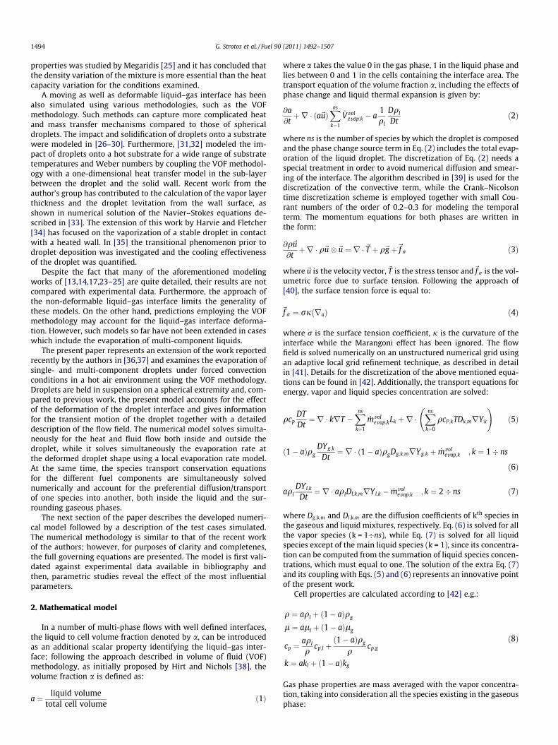
Details for the experimental set-up simulated here and used formodel validation can be found in the relevant article [51]. In brief,the droplets were placed in a wind tunnel and were held in suspen-sion at the spherical head (400 lm) of a capillary tube (200 lm),which was placed perpendicularly to the gas flow, under atmo-spheric pressure. The droplet diameter was recorded with a videocamera which was synchronized with an infrared thermo-graphicsystem for obtaining droplet’s surface temperature measurements.Since the droplet takes a deformed shape during its vaporizationprocess, the reported results refer to that of an equivalent dropletdiameter having the same volume as that of the deformed one. Athree-dimensional representation of one of the cases simulated isshown in Fig. 1, where the numerical grid with the local refinementaround the gas–liquid interface is shown, together with details of


the flow development both inside the liquid phase and the sur-rounding gas.

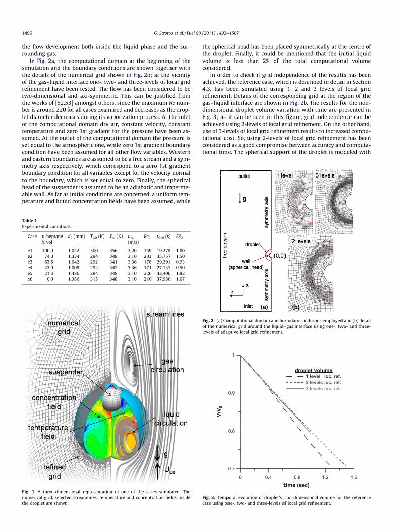
In Fig. 2a, the computational domain at the beginning of thesimulation and the boundary conditions are shown together withthe details of the numerical grid shown in Fig. 2b; at the vicinityof the gas–liquid interface one-, two- and three-levels of local gridrefinement have been tested. The flow has been considered to betwo-dimensional and axi-symmetric. This can be justified fromthe works of [52,53] amongst others, since the maximum Re num-ber is around 220 for all cases examined and decreases as the drop-let diameter decreases during its vaporization process. At the inletof the computational domain dry air, constant velocity, constanttemperature and zero 1st gradient for the pressure have been as-sumed. At the outlet of the computational domain the pressure isset equal to the atmospheric one, while zero 1st gradient boundarycondition have been assumed for all other flow variables. Westernand eastern boundaries are assumed to be a free stream and a sym-metry axis respectively, which correspond to a zero 1st gradientboundary condition for all variables except for the velocity normalto the boundary, which is set equal to zero. Finally, the sphericalhead of the suspender is assumed to be an adiabatic and imperme-able wall. As far as initial conditions are concerned, a uniform tem-perature and liquid concentration fields have been assumed, while

Table 1Experimental conditions.

Case n-heptane% vol

d0 (mm) Td,0 (K) T1 (K) u1(m/s)

Re0 tC10 (s) FR0

e1 100.0 1.052 300 356 3.20 159 19.278 1.00e2 74.0 1.334 294 348 3.10 203 35.757 1.50e3 63.5 1.042 292 341 3.36 178 29.291 0.93e4 43.0 1.008 292 342 3.36 171 27.137 0.90e5 21.3 1.486 294 348 3.10 226 42.406 1.82e6 0.0 1.386 315 348 3.10 210 37.986 1.67

Fig. 1. A three-dimensional representation of one of the cases simulated. Thenumerical grid, selected streamlines, temperature and concentration fields insidethe droplet are shown.

the spherical head has been placed symmetrically at the centre ofthe droplet. Finally, it could be mentioned that the initial liquidvolume is less than 2% of the total computational volumeconsidered.

In order to check if grid independence of the results has beenachieved, the reference case, which is described in detail in Section4.3, has been simulated using 1, 2 and 3 levels of local gridrefinement. Details of the corresponding grid at the region of thegas–liquid interface are shown in Fig. 2b. The results for the non-dimensional droplet volume variation with time are presented inFig. 3; as it can be seen in this figure, grid independence can beachieved using 2-levels of local grid refinement. On the other hand,use of 3-levels of local grid refinement results to increased compu-tational cost. So, using 2-levels of local grid refinement has beenconsidered as a good compromise between accuracy and computa-tional time. The spherical support of the droplet is modeled with

Fig. 2. (a) Computational domain and boundary conditions employed and (b) detailof the numerical grid around the liquid–gas interface using one-, two- and three-levels of adaptive local grid refinement.

0 0.4 0.8 1.2 1.6

time (sec)

0.7

0.8

0.9

1

V/V 0

droplet volume1 level loc. ref.2 levels loc. ref.3 levels loc. ref.

Fig. 3. Temporal evolution of droplet’s non-dimensional volume for the referencecase using one-, two- and three-levels of local grid refinement.


an unstructured base grid. This resulted in a numerical grid ofapproximately 4500 cells at the beginning of the simulation; thecell size at the interface region is approximately 2.6% of the dropletradius; simulations using a uniform grid having the resolution ofthe interface would require approximately 315,000 cells. Depend-ing on each case, the simulations can last approximately 1–3 CPUmonths; this is mainly due to the time step limitation of the VOFmethodology, which requires small Courant number of the orderof 0.2–0.3 in order to avoid numerical diffusion.

4. Results and discussion

4.1. Model validation

In this section the numerical model using the VOF methodologyis validated against the experimental data reported in [51] for thecases described above; the relevant conditions are summarized inTable 1. The temporal evolution of the non-dimensionalised

Fig. 4. (a and b) Numerical prediction of the temporal evolut

droplet squared diameter for all cases examined is presented inFig. 4a and b, while in Fig. 4c–e the temporal evolution of meandroplet temperature is presented for the cases in which experi-mental data were available. Furthermore, along with the presentpredictions, the predictions reported by Daïf et al. [51], Torreset al. [54], and Zeng and Lee [55], who used one-dimensional mod-els are presented together with the predictions of [56]; the latterhave used a two-dimensional model to account for the Hill’s vor-tex. Predictions for the droplet size are in good agreement withthe experimental data for the rich in n-heptane droplets; somedeviations can be observed at the latter stages of the process inwhich the less volatile n-decane dominates the phenomenon. Thesame trend is also observed for the predicted droplet temperature.The prediction for the wet-bulb temperature of the droplet at thelater stages of evaporation is overestimated approximately by6 �C. On the other hand, this overestimation has been also observedin most of the previous studies and may be attributed to thephysical properties library values used, as numerous studies non

ion of droplet size and (c–e) mean droplet temperature.


reported here have indicated. The physical processes taking placeduring multi-component droplet evaporation will be discussed indetail in Sections 4.3 and 4.4, while the influence of specific param-eters in Section 4.5. An extended investigation of the physical pro-cesses and the flow field regimes for the case e2, can be found in[36].

4.2. Droplet equilibrium position and droplet deformation

Before proceeding to the detailed transport phenomenadescription, it is important to mention that the VOF methodologyemployed here predicts that the droplet is moving on the sus-pender as a result of gravity and aerodynamic forces while it issimultaneously being held by the suspender due to the adhesionforces. Since there were no available experimental pictures, thewettability of the liquid with the solid suspender was taken intoconsideration by setting a typical contact angle of n-decane intouch with glass, since the volatile n-heptane vaporizes faster,leaving the n-decane behind towards the later stages of the pro-cess. The advancing and receding contact angle values used are90 and 10 degrees, respectively. Initially, the spherical suspenderlies at the centre of the droplet, as shown on Fig. 5a. In the workof [17] the droplet was assumed to be motionless despite the ac-tion of two forces acting initially on the droplet, namely the drop-let’s weight (B) and drag force due to air flow (FD). In the presentstudy, an extension of this work is considered by allowing thedroplet to move according to the forces acting on it. The ratio ofthe magnitude of these two forces, denoted here as FR, providesat every time step an indication for the droplet movement direc-tion. Depending on FR, the droplet can move in the direction ofgravity or the opposite one. The value of FR can be calculated usingthe drag coefficient as in [12] as:

FR ¼ BFD¼ mg

cD12 qg;1u2

1p4 d2 ¼

4qldg3qg;1u2

1cD; cD

24Re

1þ 16

Re2=3� �

ð16Þ

Fig. 5. Droplet movement and equilibrium position for case e1.

Fig. 6. Droplet equilibrium position a

For the pure n-heptane droplet (case e1) the ratio of the forces act-ing initially on the droplet is FR0 � 1.0, indicating that initially thedroplet’s weight is almost equal to the drag force. As the dropletstarts to evaporate, it becomes lighter and thus, it is moving inthe direction of the flow, as shown in Fig. 5b, until it reaches withina short period of time the equilibrium position shown on Fig. 5c.Adhesion forces oppose droplet detachment from the surface; thedroplet remains attached to the suspender for the rest of the evap-oration process (Fig. 5d–f) while its centre of mass recedes towardsthe spherical head.

For the case of the larger mixture droplet (case e2), the initialforce ratio is FR0 = 1.50, thus the droplet’s weight is now greaterthan the aerodynamic drag force. As a result, the droplet movesin the direction of gravity, which is shown in Fig. 6b, until itreaches again the equilibrium position of Fig. 6c. As further vapor-ization results to loss of liquid mass, the suspended droplet be-comes gradually lighter and at the time instant of Fig. 6d, thedrag force becomes again greater than the droplet’s weight, simi-larly to the previously described case. From this time onwards,the droplet moves to the direction of the flow, as shown inFig. 6e and f, until its complete vaporization. It is interesting to no-tice that, in this case, a small meniscus is formed at the upper partof the suspender, as shown in Fig. 6d. The formation process of thismeniscus can be explained with the aid of Fig. 6g, which shows thedimensionless pressure, defined as p� ¼ ðp� p1Þ=ð12 qg;1u2

1Þ, to-gether with the flow streamlines just before the creation of themeniscus. In the downstream part of the droplet, increased pres-sures can be observed together with the formation of two rela-tively small-scale recirculation zones with opposite rotationalmotion. These two opposite rotating fluid zones and the presenceof the suspender lead to the formation of a liquid neck on the solidsurface; finally, the liquid present to the right-hand-side of theneck pinches off, creating a meniscus at the rear part of thesuspender.

The temporal motion of the centre of liquid volume for all casesexamined is presented in Fig. 7a. As it can be seen, the droplets ofcases e1, e3 and e4 for which FR0 is less than unity, are moving inthe direction of the flow while for the rest of the cases the dropletmoves in the direction of gravity. The abrupt movement of thedroplet corresponding to case e2 is also shown, while the wavyform of curves reveal the small oscillatory motion of droplets. Onthe other hand, as already mentioned, droplets deform as it canbe seen for example Fig. 6c. A measure of their deformation canbe estimated by comparing the instantaneous droplet surface areawith that of a sphere having the same volume. Thus, the factor sph,which is always greater than one, is used:

Sph ¼ AliqðtÞAsphereðtÞ

PcellsðjrajVcellÞ

pd2 ð17Þ

nd meniscus creation for case e2.

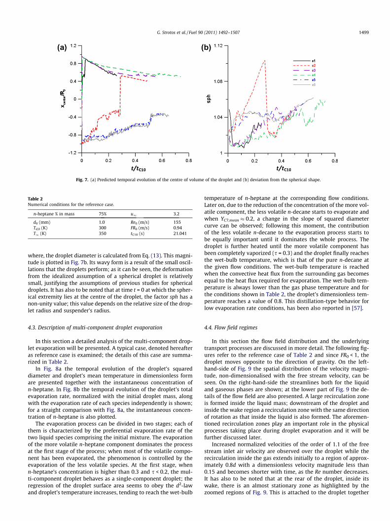
Fig. 7. (a) Predicted temporal evolution of the centre of volume of the droplet and (b) deviation from the spherical shape.

Table 2Numerical conditions for the reference case.

n-heptane % in mass 75% u1 3.2

d0 (mm) 1.0 Re0 (m/s) 155Td,0 (K) 300 FR0 (m/s) 0.94T1 (K) 350 tC10 (s) 21.041


where, the droplet diameter is calculated from Eq. (13). This magni-tude is plotted in Fig. 7b. Its wavy form is a result of the small oscil-lations that the droplets perform; as it can be seen, the deformationfrom the idealized assumption of a spherical droplet is relativelysmall, justifying the assumptions of previous studies for sphericaldroplets. It has also to be noted that at time t = 0 at which the spher-ical extremity lies at the centre of the droplet, the factor sph has anon-unity value; this value depends on the relative size of the drop-let radius and suspender’s radius.

4.3. Description of multi-component droplet evaporation

In this section a detailed analysis of the multi-component drop-let evaporation will be presented. A typical case, denoted hereafteras reference case is examined; the details of this case are summa-rized in Table 2.

In Fig. 8a the temporal evolution of the droplet’s squareddiameter and droplet’s mean temperature in dimensionless formare presented together with the instantaneous concentration ofn-heptane. In Fig. 8b the temporal evolution of the droplet’s totalevaporation rate, normalized with the initial droplet mass, alongwith the evaporation rate of each species independently is shown;for a straight comparison with Fig. 8a, the instantaneous concen-tration of n-heptane is also plotted.

The evaporation process can be divided in two stages; each ofthem is characterized by the preferential evaporation rate of thetwo liquid species comprising the initial mixture. The evaporationof the more volatile n-heptane component dominates the processat the first stage of the process; when most of the volatile compo-nent has been evaporated, the phenomenon is controlled by theevaporation of the less volatile species. At the first stage, whenn-heptane’s concentration is higher than 0.3 and s < 0.2, the mul-ti-component droplet behaves as a single-component droplet; theregression of the droplet surface area seems to obey the d2-lawand droplet’s temperature increases, tending to reach the wet-bulb

temperature of n-heptane at the corresponding flow conditions.Later on, due to the reduction of the concentration of the more vol-atile component, the less volatile n-decane starts to evaporate andwhen YC7,mean � 0.2, a change in the slope of squared diametercurve can be observed; following this moment, the contributionof the less volatile n-decane to the evaporation process starts tobe equally important until it dominates the whole process. Thedroplet is further heated until the more volatile component hasbeen completely vaporized (s = 0.3) and the droplet finally reachesthe wet-bulb temperature, which is that of the pure n-decane atthe given flow conditions. The wet-bulb temperature is reachedwhen the convective heat flux from the surrounding gas becomesequal to the heat flux required for evaporation. The wet-bulb tem-perature is always lower than the gas phase temperature and forthe conditions shown in Table 2, the droplet’s dimensionless tem-perature reaches a value of 0.8. This distillation-type behavior forlow evaporation rate conditions, has been also reported in [57].

4.4. Flow field regimes

In this section the flow field distribution and the underlyingtransport processes are discussed in more detail. The following fig-ures refer to the reference case of Table 2 and since FR0 < 1, thedroplet moves opposite to the direction of gravity. On the left-hand-side of Fig. 9 the spatial distribution of the velocity magni-tude, non-dimensionalised with the free stream velocity, can beseen. On the right-hand-side the streamlines both for the liquidand gaseous phases are shown; at the lower part of Fig. 9 the de-tails of the flow field are also presented. A large recirculation zoneis formed inside the liquid mass; downstream of the droplet andinside the wake region a recirculation zone with the same directionof rotation as that inside the liquid is also formed. The aforemen-tioned recirculation zones play an important role in the physicalprocesses taking place during droplet evaporation and it will befurther discussed later.

Increased normalized velocities of the order of 1.1 of the freestream inlet air velocity are observed over the droplet while therecirculation inside the gas extends initially to a region of approx-imately 0.8d with a dimensionless velocity magnitude less than0.15 and becomes shorter with time, as the Re number decreases.It has also to be noted that at the rear of the droplet, inside itswake, there is an almost stationary zone as highlighted by thezoomed regions of Fig. 9. This is attached to the droplet together

Fig. 8. (a) Predicted temporal evolution of droplet’s size and droplet’s mean temperature and (b) predicted evaporation rate of each species and total evaporation rate. In bothfigures the concentration of n-heptane is also presented.

Fig. 9. Total velocity magnitude (left-hand-side) and streamlines (right-hand-side) for the reference case.


with the formation of small cellular zones. The thickness of thiszone is approximately 0.04d0 and remains almost constant in time.In this region there is high vapor concentration values and lowvelocity values.

Compared to the length of the recirculation region formed be-hind a solid sphere under steady-state flow conditions, the pre-dicted recirculation flow length of the evaporating droplet is

much smaller for the same Reynolds number. This is mainly dueto the vortex motion of the liquid mass inside the droplet, whichretards flow separation towards the rear of the droplet and sup-presses the length of the wake, as also reported previously in [2].The dependence of the recirculation length on Reynolds numberis shown in Fig. 10c for some of the cases examined; the experi-mental data of [58] for a solid sphere are also shown. The Reynolds

Fig. 10. (a) Streamlines for low Reynolds number, (b) streamlines for higher Reynolds number and (c) dependence of the recirculation length with Re number.


number used is based on the relative liquid–gas velocity accordingto the estimation of maximum liquid surface velocity presented in[12]. This assumption takes into consideration both the ratio of li-quid to gas viscosities and the evaporation rate of the droplet. Asatisfactory approximation of the wake length is also shown inFig. 10c. In Fig. 10a and b, the flow field for two cases with differentRe numbers is shown; for Re values smaller than 30, no recircula-tion zone in the gaseous phase has been observed. The velocitiesinside the liquid phase are much smaller than the velocities inthe gaseous phase; their magnitude does not exceed 6% of freestream velocity which is in agreement with the works of [59,60].In these works, a vortex model was developed and it was provedthat the velocities inside the liquid are less than one order of mag-nitude compared to the free stream velocity. Inside the liquid tworecirculation zones are formed; the bigger one occupies most of thedroplet volume while the smaller one is formed at the rear of thedroplet and it is clearly shown in the magnified regions of Fig. 9.According to [2], the second recirculation is often observed, but itis too small and can be ignored. Thus, the flow inside the droplet

Fig. 11. Radial distribution of (a) dimensionless velocity and dimensionless vo

can be approximated as a Hill’s vortex; this comment is justifiedfor the initial stages of the droplet evaporation. The simulationsperformed here reveal that the length of the second vortex alongthe x-axis, is approximately 0.04–0.06d0 and remains almost con-stant with time; this length is very small at the initial stages ofthe process when compared to the initial droplet diameter, but itbecomes progressively larger and larger; at s = 0.55 its length is�0.11d. The same trend for the second vortex was also observedin [17]. The centre of the big vortex in the x-axis does not coincidewith the corresponding centre of liquid volume, mainly due to thepresence of the solid suspender and the formation of the secondaryvortex. Theoretically, based on the Hill’s vortex model (see [2]among others), the vortex centre should be located at 90� fromthe front stagnation point and at a distance of R=

ffiffiffi2p

from the axisof symmetry. The present simulations reveal that the centre of thebig vortex moves during evaporation from 87� to 101�, while itsdistance from the axis of symmetry varies from 0.73 to 0.83R;these values are slightly higher from the theoretical ones thatignore the presence of the suspender.

rticity and (b) dimensionless stream-function through the vortex centre.


The distribution of the dimensionless x-component velocitycomponent ux/u1 and the dimensionless vorticity are shown inFig. 11a; these profiles have been extracted on the radial directionpassing through the centre of the main liquid vortex while theplotted curves correspond to five time instances. Similarly, the dis-tribution of the dimensionless stream-function w/(u1R2) along thesame location and times is shown in Fig. 11b; the vorticity and thestream-function are non-dimensionalised with the instantaneousequivalent droplet radius. The absolute values of the dimensionlessvelocity and stream-function become smaller as time progressesdue to Re number regression. This is in accordance with the find-ings of [14,17], while the stream-function reaches its maximumat the centre of the vortex. On the other hand, the dimensionlessvorticity varies almost linearly in the radial direction; the slightlydistorted values near the liquid–gas interface are only numericalartifacts arising from VOF-based discretization of the liquid–gasinterface.

Fig. 12. Non-dimensional temperatu

Fig. 13. Vapor pressure field non-dimensionalised with saturation pressure for each spetime instances of s = 0.048 and s = 0.238.

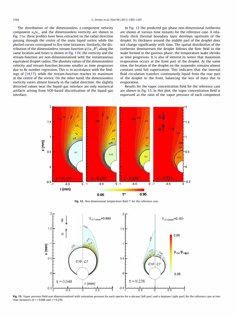
In Fig. 12 the predicted gas phase non-dimensional isothermsare shown at various time instants for the reference case. A rela-tively thick thermal boundary layer develops upstream of thedroplet. Its thickness around the middle part of the droplet doesnot change significantly with time. The spatial distribution of theisotherms downstream the droplet follows the flow field in thewake formed in the gaseous phase; the temperature wake shrinksas time progresses. It is also of interest to notice that maximumevaporation occurs at the front part of the droplet. At the sametime, the location of the droplet on the suspender remains almostconstant until full vaporization. This indicates that the internalfluid circulation transfers continuously liquid from the rear partof the droplet to the front, balancing the loss of mass due toevaporation.

Results for the vapor concentration field for the reference caseare shown in Fig. 13. In this plot, the vapor concentration field isexpressed as the ratio of the vapor pressure of each component

re field T� for the reference case.

cies for n-decane (left part) and n-heptane (right part) for the reference case at two


normalized with the corresponding saturation vapor pressure ofthe same component at the same cell temperature. This normaliza-tion provides a better insight of the physical phenomenon, sincethe actual mass fraction of each component in the gaseous phaseexhibits very different values due to pure species volatilitydifference. In Fig. 13, the left-hand-side corresponds to n-decane’snormalized vapor pressure and the right-hand-side represents thesame magnitude but for the n-heptane component. Values of thisrelative saturation ratio cannot exceed the corresponding valuesof liquid molecular fraction of each component. At the initial stagesof the process, e.g. s = 0.048 when the more volatile n-heptane isvaporizing faster, the normalized vapor pressure exhibits large val-ues at the gas–liquid interface region. The opposite behavior is ob-served for the less volatile n-decane component. Similarly to thethermal boundary layer and velocity wake of the gas flow, the con-centration boundary layer and its wake have a similar topology;strong concentration gradients develop at the front part of thedroplet while further downstream the spatial distribution is af-fected by the presence of the recirculation zone. It is also worth-while to refer that the spatial distribution of the concentrationfields for both species exhibit similarities but with a time delay.

In Fig. 14 the temperature field and the n-heptane concentra-tion fields inside the liquid droplet are presented for the referencecase on the left- and right-hand-sides, respectively, at two time in-stances. Due to low evaporation rate, the thermal and concentra-tion gradients that develop inside the liquid mass are quiteweak; so it has been considered more convenient to plot the differ-

Fig. 14. Temperature field (left-hand-side) and concentration field (right-hand-side) ins = 0.238.

Table 3Numerical conditions for the parametric investigation.

Case name Less volatile More volatile Y0

Ref. C10 C7 0.75C7 0% 0

C7 25% 0.25C7 50% 0.5

C7 100% 1T = 400 KT = 450 K

d = 0.2 mmd = 0.1 mm

C10–C6 C6 0.75C10–C8 C8 0.75C10–C9 C9 0.75

ence of their magnitude from the corresponding mean value at thesame time together with the corresponding mean mass averagedvalue for the temperature and the n-heptane concentration. As itcan be seen, the relatively low evaporation rate in combinationwith the homogenization of the liquid composition caused by theinternal liquid circulation [61], results to almost negligible differ-ences from the mean values. Furthermore, small temperature andconcentration differences imply that neglecting the Marangoni ef-fect on surface tension is a reasonable hypothesis, while infiniteconductivity and infinite diffusivity models could be used for fastpredictions. Despite the fact that the temperature and concentra-tion gradients inside the droplet are small, the numerical findingof [23] is verified by the present predictions; inside the liquid coreslightly increased values of the concentration of the volatile n-hep-tane are observed throughout the evaporation process. This resultsfrom the combination of the internal liquid circulation and the dif-fusion process of n-heptane inside the liquid. At later times, lack ofthe more volatile specie is observed in the rear part of the droplet.

4.5. Parametric investigation of droplet evaporation

Following model validation, a set of parametric studies is per-formed in order to reveal in detail the influence of various param-eters on the complicated thermo-fluid dynamics and phase-changeprocesses taking place during the multi-component evaporationprocess. The parameters investigated include the effect of initialconcentration, droplet diameter, gas temperature and species

side the liquid phase for the reference case at two time instances of s = 0.048 and

d0 (mm) T1 (K) Re0 FR0 tC10 (s)

1.0 350 155 0.94 21.041

400 123 0.97 7.5758450 101 0.99 4.4975

0.2 31 0.08 1.5340.1 16 0.03 0.4769

Fig. 15. Predicted temporal evolution of (a) droplet’s size and (b) droplet’s mean dimensionless temperature, showing the influence of the initial concentration in n-heptane.


volatility difference. The reference case of Table 2 is common for allthe tests performed while only one parameter is changing in eachnumerical test. Such studies have also been presented before in theliterature using zero-, one- and two-dimensional models but is wasconsidered of interest to verify past finding using the complete dif-ferential flow, heat transfer and phase-change equations employedhere.

Initially, the effect of the volatile n-heptane concentration in themixture is examined. Then, droplets consisting of 75% by mass ofn-heptane and variable heavier components are considered andthe effect of droplet size and gas phase temperature is investigated.The cases examined are summarized in Table 3; on this table, blankcells denote values equal to those of the reference case which areshown on the top row of the table.

4.5.1. Influence of droplet mixture compositionDroplets with 1 mm diameter and 300 K initial temperature are

exposed in a convective environment of 350 K temperature, underatmospheric pressure and 3.2 m/s free stream velocity. Five initialmass concentrations of n-heptane in liquid are studied: 100% (pureheptane), 75% (reference case), 50%, 25% and 0% (pure decane). Thetime is non-dimensionalized with the time-scale corresponding tothe lifetime of pure decane, which is tC10 = 21.041 s for the givenconditions.

Fig. 15 shows the temporal evolution of the droplet’s squareddiameter and its mean dimensionless temperature. The evapora-tion of the pure species droplet obeys the d2-law, while the sizeregression of the pure n-decane droplet slightly deviates fromthe d2-law at the initial stages of the evaporation process due toinitial droplet heat-up. The mean volume-averaged temperatureof the pure species droplet is continuously increasing but at adecreasing rate, until it reaches the wet-bulb temperature andremaining constant hereafter.

The transitional behavior described in Section 4.3 is also ob-served here and becomes more intense with the increase of the ini-tial concentration of the volatile component. This is evident fromthe marked change of the slope of the curve describing the sizeregression of the 75% mixture compared to the corresponding ofthe 25% mixture. This is in agreement with the temperature curves,where the rich volatile-component mixture exhibits a nearly iso-thermal period (s � 0.1); contrary to that, this behavior tends tovanish when the initial concentration of the volatile componentis decreasing.

The evaporation rate of the droplet is shown in Fig. 16a; as itcan be seen, it increases with increasing concentration of the vola-tile n-heptane component in the mixture. Its temporal variationsexhibits a peak followed by a continuous decrease. This behavioris due to the fact that the evaporation rate increases with droplettemperature and droplet size. During the evolution of the phenom-enon, droplet’s temperature increases but droplet’s diameterdecreases. Furthermore, the evaporation of mixture droplets exhib-its a distillation-type behavior as already described in Section 4.3.This is valid for all mixtures irrespectively of the initial concentra-tion of the volatile component. The later can be justified by exam-ining Fig. 16b in which the contribution of the volatilen-heptane in the total evaporation rate is presented. At the initialstages of the evaporation process and irrespectively of the initialconcentration of the volatile n-heptane component, the totalevaporation rate is defined mainly by the evaporation of the morevolatile component.

Another interesting point that deserves to be addressed is thatthe final wet-bulb temperature for all droplets containing n-decaneis the same, irrespectively of the initial concentration of n-heptane.This was expected since at the later stages of evaporation when thewet-bulb temperature is reached, only the less volatile n-decaneremains and the droplet behaves as if it was a single-componentdroplet. Numerically, this is achieved by taking into considerationthe species diffusion term for multi-component mixtures appear-ing to the right-hand-side of the energy Eq. (5):

r �X

k

qcP;kTDk;mrYk

!ð18Þ

This term, must be included in the energy equation even if asingle-component droplet is simulated, since the surrounding gasis a mixture of air and vapor. The influence of ignoring this termin single-component droplets can be found in [37] and leads todifferent wet-bulb temperatures for pure species and mixtures forthe same flow conditions.

4.5.2. Influence of droplet diameter, gas temperature and speciesvolatility

In this section, multi-component droplets containing 75% bymass n-heptane are examined in order to reveal the effect ofdroplet size, gas phase temperature and species volatility differ-ence. Three droplet diameters are studied: 0.1 mm, 0.2 mm and1.0 mm (reference case), while it is important to notice that the

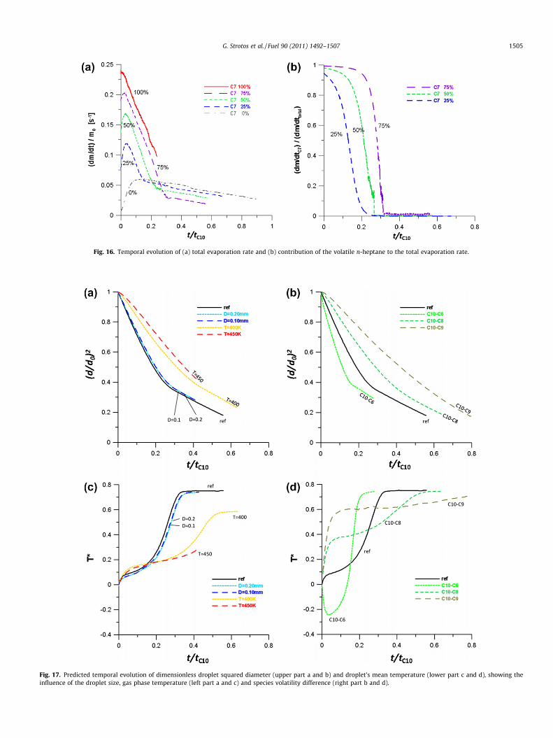
Fig. 16. Temporal evolution of (a) total evaporation rate and (b) contribution of the volatile n-heptane to the total evaporation rate.

Fig. 17. Predicted temporal evolution of dimensionless droplet squared diameter (upper part a and b) and droplet’s mean temperature (lower part c and d), showing theinfluence of the droplet size, gas phase temperature (left part a and c) and species volatility difference (right part b and d).



ratio of the initial droplet diameter to the suspender diameter, re-mains unchanged. Similarly, three surrounding air temperaturesare considered: 350 K (reference case), 400 K and 450 K. It is ofimportance to emphasize here that even for the higher tempera-ture value, equilibrium thermodynamic conditions apply. Finally,binary droplets consisting of n-decane and four different chemicalspecies are tested. The dissolved in n-decane species are n-hexane,n-heptane (reference case), n-octane and n-nonane. In followingFig. 17 the temporal evolution of non-dimensional droplet’ssquared diameter and dimensionless droplet temperature isshown, while the time axis is normalized with n-decane dropletlifetime.

From Fig. 17 it is concluded that in dimensionless form, theevaporation of multi-component droplets exhibits the same behav-ior for all cases examined. The d2-law for each component sepa-rately is confirmed for all cases, while the wet-bulb temperatureis mainly controlled by the gas phase temperature. Droplet sizedoes not affect the transitional behavior of droplet evaporation, de-spite the fact that the total evaporation time of a droplet is propor-tional to d2

0. The transitional behavior tends to disappear withincreasing gas phase temperature and decreasing species volatilitydifference, which is in agreement with the findings of [57]. In-crease of the gas phase temperature results to decreased actualdroplet lifetime and increased wet-bulb temperature in dimen-sional units. On the other hand, in non-dimensional units, theopposite behavior is observed; dimensionless wet-bulb tempera-ture decreases with increasing gas phase temperature.

For the cases with variable species volatility difference, the mix-ture containing n-hexane experiences an intense transitionalbehavior. On the other hand, the n-nonane mixture exhibits a veryweak transitional behavior. The droplet’s temperature reaches thesame wet-bulb temperature for all mixtures, since the less volatilen-decane controls the second stage of evaporation. It is interestingto observe that the temperature of the n-hexane’s mixture, initiallydecreases and then increases; this is due to the wet-bulbtemperature of the pure n-hexane, which is lower than the initialtemperature of the droplet.

Finally, it has to be noted that the case with 450 K gas phasetemperature is characterized by a high evaporation rate; the laterin combination with the accumulation of numerical errors result-ing from the large number of computational time steps, resultedin smearing and diffusion of the gas–liquid interface. So the simu-lation was stopped earlier compared to other runs, since from thispoint and afterwards, predictions were not considered reliable.This problem was partly suppressed by using even smaller Courantnumber and a liquid–gas interface sharpening technique, which re-duced the numerical diffusion at the interface.

5. Conclusions

A Navier–Stokes equation numerical methodology coupled withan evaporation model and the VOF methodology, utilizing anunstructured dynamically adapting computational grid, have beenused to numerically predict the evaporation process of a dropletconsisting of one or two components at various concentrations.The droplet was suspended in the spherical extremity of a capillarytube under convective flow conditions. The model used has beeninitially validated against experimental data, referring to both sin-gle- and binary mixture droplets, showing good agreement.

The VOF methodology proved to be capable of predicting drop-let motion, droplet shape and droplet final position on the solidsuspender as also accurate evaporation rates both for single andbinary mixtures. The components of the binary droplet are prefer-entially evaporated and a distillation-type evaporation processtakes place. A d2-law type of evaporation is observed in two stages.

Initially the droplet tends to reach a wet-bulb temperature sinceevaporation is dominated by the more volatile species; then aheat-up follows and when the more volatile n-heptane has beennearly fully vaporized, droplet’s temperature reaches the wet-bulbtemperature of pure n-decane. This transitional behavior is inde-pendent of the droplet size and tends to be more intense for richin volatile mixtures, as also in cases with a low evaporation rateand large volatility differences between mixture species.

A detailed description of the flow variables both in the gaseousand the liquid phases has been presented. The recirculation zonesformed inside the liquid and gas phases play an important role onthe spatial distribution of flow variables. In the gas phase, the recir-culation zone is much smaller compared to the one correspondingto a solid sphere with the same Reynolds number. Its length re-duces with time due to droplet evaporation and thus to Re numberreduction. Inside the liquid two recirculation zones are formedcomprising a main vortex and a smaller one; the latter occupiesan almost constant with time length at the rear part of the droplet,thus increasing its relative size compared to the decreasing dropletdiameter. The vorticity of the main vortex reduces from the dropletsymmetry axis to the droplet surface but remains almost constantwith time. The presence of the solid suspender along with theoscillations of the droplet moves the centre of the big vortex fur-ther off the symmetry axis and towards the rear stagnation point.Finally, a vapor layer consisting of organized vapor cells seems tobe formed around the evaporating droplet having a size of 0.04d0.

Strong thermal and concentration gradients are formed at thefront of the droplet, while downstream the corresponding spatialdistribution is affected from the recirculation inside the gas phase.Inside the droplet, the temperature and concentration fieldsproved to be almost uniform due to the low evaporation rate ofthe cases examined. This justifies the use of infinite conductivityand infinite diffusivity models (ICM and IDM) for predicting drop-let evaporation.

References

[1] Clift R, Grace JR, Weber ME. Bubbles, drops and particles. New York: AcademicPress; 1978.

[2] Sirignano WA. Fluid dynamics and transport of droplets and sprays. CambridgeUniversity Press; 1999.

[3] Bird RB, Stewart WE, Lightfoot EN. Transport phenomena. 2nd ed. NewYork: Wiley; 2002.

[4] Givler SD, Abraham J. Supercritical droplet vaporization and combustionstudies. Prog Energy Combust Sci 1996;22:1–28.

[5] Miller RS, Harstad K, Bellan J. Evaluation of equilibrium and non-equilibriumevaporation models for many-droplet gas–liquid flow simulations. Int JMultiphase Flow 1998;24:1025–55.

[6] Bellan J. Supercritical (and subcritical) fluid behavior and modeling: drops,streams, shear and mixing layers, jets and sprays. Prog Energy Combust Sci2000;26:329–66.

[7] Sazhin SS. Advanced models of fuel droplet heating and evaporation. ProgEnergy Combust Sci 2006;32:162–214.

[8] Godsave GAE. Burning of fuel droplets. In: 4th international symposium oncombustion. Baltimore: The Combustion Institute; 1953. p. 818–30.

[9] Spalding DB. The combustion of liquid fuels. In: 4th international symposiumon combustion. Baltimore: The Combustion Institute; 1953. p. 847–64.

[10] Law CK. Unsteady droplet combustion with droplet heating. Combust Flame1976;26:17–22.

[11] Law CK, Sirignano WA. Unsteady droplet combustion with droplet heating – II:conduction limit. Combust Flame 1977;28:175–86.

[12] Abramzon B, Sirignano WA. Droplet vaporization model for spray combustioncalculations. Int J Heat Mass Transf 1989;32:1605–18.

[13] Haywood RJ, Nafziger R, Renksizbulut M. Detailed examination of gas andliquid phase transient processes in convective droplet evaporation. J HeatTransf 1989;111:495–502.

[14] Chiang CH, Raju MS, Sirignano WA. Numerical analysis of convecting,vaporizing fuel droplet with variable properties. Int J Heat Mass Transf1992;35:1307–24.

[15] Megaridis CM. Comparison between experimental measurements andnumerical predictions of internal temperature distributions of a dropletvaporizing under high-temperature convective conditions. Combust Flame1993;93:287–302.

[16] Wong SC, Lin AC. Internal temperature distributions of droplets vaporizing inhigh-temperature convective flows. J Fluid Mech 1992;237:671–87.


[17] Shih AT, Megaridis CM. Suspended droplet evaporation modeling in a laminarconvective environment. Combust Flame 1995;102:256–70.

[18] Lasheras JC, Fernandez-Pello AC, Dryer FL. Experimental observations on thedisruptive combustion of free droplets of multicomponent fuels. Combust SciTechnol 1980;22:195–209.

[19] Law CK. Multicomponent droplet combustion with rapid internal mixing.Combust Flame 1976;26:219–33.

[20] Law CK. Internal boiling and superheating in vaporizing multicomponentdroplets. AIChE J 1978;24:626–32.

[21] Maqua C, Castanet G, Lemoine F. Bicomponent droplets evaporation:temperature measurements and modelling. Fuel 2008;87:2932–42.

[22] Sazhin SS, Elwardany A, Krutitskii PA, Castanet G, Lemoine F, Sazhina EM, et al.A simplified model for bi-component droplet heating and evaporation. Int JHeat Mass Transf 2010;53:4495–505.

[23] Megaridis CM, Sirignano WA. Numerical modeling of a vaporizingmulticomponent droplet. Int Symp Combust 1990;23:1413–21.

[24] Megaridis CM, Sirignano WA. Multicomponent droplet vaporization in alaminar convective environment. Combust Sci Technol 1993;87:27–44.

[25] Megaridis CM. Liquid-phase variable property effects in multicomponentdroplet convective evaporation. Combust Sci Technol 1993;92:291–311.

[26] Liu H, Lavernia EJ, Rangel RH. Numerical simulation of substrate impact andfreezing of droplets in plasma spray processes. J Phys D: Appl Phys 1993;26:1900–8.

[27] Pasandideh-Fard M, Bhola R, Chandra S, Mostaghimi J. Deposition of tindroplets on a steel plate: simulations and experiments. Int J Heat Mass Transf1998;41:2929–45.

[28] Zheng LL, Zhang H. An adaptive level set method for moving-boundaryproblems: application to droplet spreading and solidification. Numer HeatTransf Part B-Fundam 2000;37:437–54.

[29] Pasandideh-Fard M, Chandra S, Mostaghimi J. A three-dimensionalmodel of droplet impact and solidification. Int J Heat Mass Transf 2002;45:2229–42.

[30] Ghafouri-Azar R, Shakeri S, Chandra S, Mostaghimi J. Interactions betweenmolten metal droplets impinging on a solid surface. Int J Heat Mass Transf2003;46:1395–407.

[31] Harvie DJE, Fletcher DF. A hydrodynamic and thermodynamic simulation ofdroplet impacts on hot surfaces, Part II: validation and applications. Int J HeatMass Transf 2001;44:2643–59.

[32] Harvie DJE, Fletcher DF. A hydrodynamic and thermodynamic simulation ofdroplet impacts on hot surfaces, Part I: theoretical model. Int J Heat MassTransf 2001;44:2633–42.

[33] Nikolopoulos N, Theodorakakos A, Bergeles G. A numerical investigation of theevaporation process of a liquid droplet impinging onto a hot substrate. Int JHeat Mass Transf 2007;50:303–19.

[34] Strotos G, Gavaises M, Theodorakakos A, Bergeles G. Numerical investigationon the evaporation of droplets depositing on heated surfaces at low Webernumbers. Int J Heat Mass Transf 2008;51:1516–29.

[35] Strotos G, Gavaises M, Theodorakakos A, Bergeles G. Numerical investigationof the cooling effectiveness of a droplet impinging on a heated surface. Int JHeat Mass Transf 2008;51:4728–42.

[36] Strotos G, Gavaises M, Theodorakakos A, Bergeles G. Evaporation of asuspended multicomponent droplet under convective conditions. In: ICHMT,Marrakech, Morocco; 2008.

[37] Strotos G, Gavaises M, Theodorakakos A, Bergeles G. Influence of speciesconcentration on the evaporation of suspended multicomponent droplets. In:ILASS 2008, Como Lake, Italy; 2008.

[38] Hirt CW, Nichols BD. Volume of fluid (Vof) method for the dynamics of freeboundaries. J Comput Phys 1981;39:201–25.

[39] Ubbink O, Issa RI. A method for capturing sharp fluid interfaces on arbitrarymeshes. J Comput Phys 1999;153:26–50.

[40] Brackbill JU, Kothe DB, Zemach C. A continuum method for modeling surfacetension. J Comput Phys 1992;100:335–54.

[41] Theodorakakos A, Bergeles G. Simulation of sharp gas–liquid interface usingVOF method and adaptive grid local refinement around the interface. Int JNumer Methods Fluids 2004;45:421–39.

[42] Nikolopoulos N, Theodorakakos A, Bergeles G. Normal impingement of adroplet onto a wall film: a numerical investigation. Int J Heat Fluid Flow2005;26:119–32.

[43] Perry RH, Green DW. Perry’s chemical engineers’ handbook. 7th ed. McGraw-Hill; 1997.

[44] Poling BE, Prausnitz JM, O’Connell JP. Properties of gases and liquids. 5thed. McGraw-Hill; 2001.

[45] Fluid_Research_Company, Manual on the GFS CFD code; 2002. <www.fluid-research.com>.

[46] Nikolopoulos N, Theodorakakos A, Bergeles G. Three-dimensional numericalinvestigation of a droplet impinging normally onto a wall film. J Comput Phys2007;225:322–41.

[47] Nikolopoulos N, Theodorakakos A, Bergeles G. Off-centre binary collision ofdroplets: a numerical investigation. Int J Heat Mass Transf 2009;52:4160–74.

[48] Nikolopoulos N, Nikas K-S, Bergeles G. A numerical investigation of centralbinary collision of droplets. Comput Fluids 2009;38:1191–202.

[49] Strotos G, Nikolopoulos N, Nikas K-S. A parametric numerical study of thehead-on collision behavior of droplets. Atomization Sprays 2010;20:191–209.

[50] Ranz ME, Marshall WR. Evaporation from drops: part I. Chem Eng Prog1952;48:141–6.

[51] Daïf A, Bouaziz M, Chesneau X, Ali Cherif A. Comparison of multicomponentfuel droplet vaporization experiments in forced convection with the Sirignanomodel. Exper Thermal Fluid Sci 1999;18:282–90.

[52] Magarvey RH, Bishop RL. Transition ranges for three dimensional wakes. Can JPhys 1961;39:1418–22.

[53] Wu J-S, Faeth GM. Sphere wakes in still surroundings at intermediate Reynoldsnumbers. AAIA J 1993;31:1448–55.

[54] Torres DJ, O’Rourke PJ, Amsden AA. Efficient multicomponent fuel algorithm.Combust Theory Model 2003;7:67–86.

[55] Zeng Y, Lee CF. A model for multicomponent spray vaporization in a high-pressure and high-temperature environment. J Eng Gas Turb Power2002;124:717–24.

[56] Ozturk A, Cetegen BM. Modeling of plasma assisted formation of precipitatesin zirconium containing liquid precursor droplets. Mater Sci Eng A2004;384:331–51.

[57] Gökalp I, Chauveau C, Berrekam H, Ramos-Arroyo NA. Vaporization of misciblebinary fuel droplets under laminar and turbulent convective conditions.Atomization Sprays 1994;4:661–76.

[58] Taneda S. Experimental Investigation of the Wake behind a Sphere at LowReynolds Numbers. J Phys Soc Jpn 1956;11:1104–8.

[59] Prakash S, Sirignano WA. Liquid fuel droplet heating with internal circulation.Int J Heat Mass Transf 1978;21:885–95.

[60] Prakash S, Sirignano WA. Theory of convective droplet vaporization withunsteady heat transfer in the circulating liquid phase. Int J Heat Mass Transf1980;23:253–68.

[61] Faeth GM. Current status of droplet and liquid combustion. Prog EnergyCombust Sci 1977;3:191–224.

http://www.fluid-research.com

http://www.fluid-research.com

Numerical investigation of the evaporation of two-component droplets

Documents

Transcript of Numerical investigation of the evaporation of two-component droplets