HAL Id: hal-01653576https://hal.archives-ouvertes.fr/hal-01653576

Submitted on 1 Dec 2017

HAL is a multi-disciplinary open accessarchive for the deposit and dissemination of sci-entific research documents, whether they are pub-lished or not. The documents may come fromteaching and research institutions in France orabroad, or from public or private research centers.

L’archive ouverte pluridisciplinaire HAL, estdestinée au dépôt et à la diffusion de documentsscientifiques de niveau recherche, publiés ou non,émanant des établissements d’enseignement et derecherche français ou étrangers, des laboratoirespublics ou privés.

Humidity-insensitive water evaporation from molecularcomplex fluids

Jean-Baptiste Salmon, Frédéric Doumenc, Beatrice Guerrier

To cite this version:Jean-Baptiste Salmon, Frédéric Doumenc, Beatrice Guerrier. Humidity-insensitive water evaporationfrom molecular complex fluids. Physical Review E , American Physical Society (APS), 2017. �hal-01653576�

Humidity-insensitive water evaporationfrom molecular complex fluids

Jean-Baptiste Salmon∗

CNRS, Solvay, LOF, UMR 5258, Univ. Bordeaux, F-33600 Pessac, France.

Frederic DoumencLaboratoire FAST, Univ. Paris-Sud, CNRS, Universite Paris-Saclay, F-91405, Orsay, France, and

Sorbonne Universites, UPMC Univ Paris 06, UFR 919, F-75005 Paris, France

Beatrice GuerrierLaboratoire FAST, Univ. Paris-Sud, CNRS, Universite Paris-Saclay, F-91405, Orsay, France.

(Dated: September 14, 2017)

We investigated theoretically water evaporation from concentrated supramolecular mixtures, suchas solutions of polymers or amphiphilic molecules, using numerical resolutions of a one dimensionalmodel based on mass transport equations. Solvent evaporation leads to the formation of a concen-trated solute layer at the drying interface, which slows down evaporation in a long-time scale regime.In this regime, often referred to as the falling rate period, evaporation is dominated by diffusive masstransport within the solution, as already known. However, we demonstrate that, in this regime, therate of evaporation does not also depend on the ambient humidity for many molecular complexfluids. Using analytical solutions in some limiting cases, we first demonstrate that a sharp decreaseof the water chemical activity at high solute concentration, leads to evaporation rates which dependweakly on the humidity, as the solute concentration at the drying interface slightly depends on thehumidity. However, we also show that a strong decrease of the mutual diffusion coefficient of thesolution enhances considerably this effect, leading to nearly independent evaporation rates over awide range of humidity. The decrease of the mutual diffusion coefficient indeed induces strong con-centration gradients at the drying interface, which shield the concentration profiles from humidityvariations, except in a very thin region close to the drying interface.

I. INTRODUCTION

Water evaporation from binary molecular complexfluid solutions (polymers, amphiphilic molecules, etc.) isa common feature of many different experimental situa-tions ranging from the drying of water-borne polymericcoatings to spray-drying in food engineering [1]. For am-bient conditions and slow drying, water in the solution isat equilibrium with its vapor at the liquid-gas interface,and evaporation is driven by the vapor mass transfer to-wards the surrounding air, see Fig. 1 for the case of thedrying of a thick film [2, 3]. For low volatile solvents suchas water at ambient conditions, the rate of evaporationfrom the drying interface takes then the following form:

ρVev = k(ci − c∞), (1)

where ρ is the density of liquid water, k a mass trans-fer coefficient (m/s), ci the water vapor concentration atthe interface, and c∞ the water vapor concentration inthe surroundings [2, 3]. For the slow drying configura-tions considered here, we assume isothermal conditions.At early time scales and for dilute solutions, the low so-lute concentration within the bulk fluid hardly affects thewater chemical activity, leading thus to:

ρVev = kcsat(1− ae), (2)

∗ jean-baptiste.salmon-exterieur@solvay.com

where csat (kg/m3) is the concentration at saturation ofwater in the vapor phase for pure water, and ae the hu-midity of the ambient air [2, 3]. In this regime, also

liquid phase

gas phase

ci

c∞

ϕi

0.4

0.6

0.8

H

0 0.2 0.4 0.6 0.8 10

0.2

0.4

0.6

0.8

1

ξ ∼ D0/Vev

FIG. 1. Evaporation of a thick film. Water evaporation fromthe liquid binary mixture induces a receding of the dryinginterface at a rate Vev (m/s). Colors code for the solute con-centration within the fluid, whereas the grayscale codes forthe mass transfer within the gas phase. ξ ∼ D0/Vev is thetypical scale of the evaporation-induced concentration polar-ization layer, ci the water vapor concentration at the dryinginterface, c∞ the water concentration in surrounding ambientair, and ϕi the solute concentration within the fluid at thedrying interface.

known as the constant rate period in the context of poly-mer coatings [4–6], the evaporation rate is nearly con-stant, and depends on both the ambient humidity (termae) and mass transfer within the gas phase (term k). Wa-

2

ter evaporation, in turn, drives also a receding of the dry-ing interface, at a rate Vev owing to mass conservation.The receding of the interface consequently concentratesthe non-volatile solutes at the air-solution interface in alayer of thickness ξ ∼ D0/Vev, where D0 is the solutediffusivity in the dilute regime, see Fig. 1. Such a layer,also known as the concentration polarization layer in thefield of membrane science [7], arises from the competitionbetween diffusion and the displacement of the interface,a common feature of many different processes such asultra-filtration or drying.

In the following, we focus on experimental situationsfor which the polarization layer remains smaller than thetotal thickness H of the solution, i.e. H � D0/Vev. Sucha regime is not only key for understanding the drying ofsessile drops [8–10] or of thick films [11, 12], but also forinvestigating evaporation-driven water transport throughconcentrated supramolecular solutions [13, 14] (see be-low). At long time scales, accumulation of solutes in thepolarization layer also affects the water chemical activityat the air/fluid interface, and the latter is now at equi-librium with air saturated with water at a concentrationci = a(ϕi)csat, where ϕi is the solute concentration atthe drying interface, and a(ϕi) the corresponding waterchemical activity. Solute accumulation thus slows downthe drying kinetics as the evaporation rate now follows:

ρVev = kcsat(a(ϕi)− ae). (3)

In this regime, also known as the falling rate period in thefield of polymer coatings [4–6], ϕi increases asymptoti-cally towards ϕ? given by the local chemical equilibriuma(ϕ?) = ae, and Vev → 0 leading to a broadening of theconcentrated layer as the latter evolves as ξ ∼ D0/Vev.In this long time scales regime, the evaporation rate doesnot depend anymore on mass transfer within the vaporphase, but only on solute diffusion through the polariza-tion layer [4–6]. One still nevertheless expects that theambient humidity plays a role on the drying kinetic, as aesets the limiting concentration ϕ? at the drying interface.

However, Roger et al. investigated recently the dryingof aqueous solutions of amphiphilic molecules exhibitingself-assembled phases at high solute concentrations, formimicking the biological complexity of water evapora-tion through mammalian skins [13, 14]. Strikingly, theirexperiments demonstrated that evaporation rates fromsuch complex fluids do not depend on the humidity (atlong time scales and on a wide range ae = 0–0.95), as alsoobserved for real mammalians skins. Their main inter-pretation, strengthened by in-situ observations, relies onthe nucleation and growth of a thin concentrated phaseat the drying interface, leading to the conclusion thatself-assembly is possibly a key ingredient to explain thishumidity-insensitive regime [15].

In the present work, we show actually that evapora-tion rates do not depend on the ambient humidity ae(on a wide range) in the falling rate regime, for complexfluids such as solutions of polymers or surfactants, in-dependently on any phase transition. Surprisingly, such

a result has not been demonstrated theoretically to thebest of our knowledge, despite the large amount of pre-viously reported theoretical investigations, probably be-cause such works mainly focused on the description ofthin film drying [4–6]. We demonstrate in the following,using both numerical simulations of mass transport equa-tions and analytical solutions in some limiting cases, thatevaporation rates are nearly humidity-insensitive whentwo ingredients are encountered: (1) a sharp decreaseof the water chemical activity at high solute concentra-tion, and/or (2) a strong decrease of the mutual diffusioncoefficient of the aqueous solution at high solute con-centration. These features are commonly encounteredfor solutions of polymers and amphiphilic molecules thusemphasizing the significance of this result for processesinvolving water transport within complex fluids.

To demonstrate this result, we will consider for simplic-ity the case of a binary mixture composed of a volatilesolvent and a non-volatile solute, and we will focus moreprecisely on the model experiments shown schematicallyin Fig. 2. The solution is confined within a long cap-illary (length H) with an open end from which solventevaporates, and is connected to a reservoir at the op-posite end. We will also consider two different experi-

ae

V

XX=0

0 10

1

ϕ0

a(ϕ)

(a)

0 110−15

10−10

ϕ

D(ϕ)(m

2/s)

(b)

0 1

1

d

ϕc

D(ϕ

)

00

1

T

X

ϕ

(a)

00

1

X

ϕ

(b)

00

ϕ0

T 00

ϕ0

T∆T

H

FIG. 2. Uni-directional drying of a binary mixture within acapillary (length H). Top: solvent evaporation at a rate Vev

induces a flow which enriches the tip with solutes (colors codefor the solute concentration). ϕ0 is the concentration imposedat the inlet of the capillary, ae the ambient humidity. (a) and(b) Two different experimental configurations. (a) Growingconcentration polarization layer, i.e. fixed concentration ϕ0

in the reservoir: solutes accumulate continuously within thecapillary (see inset). (b) Steady concentration polarizationlayer obtained when imposing ϕ0 = 0 in the reservoir after adelay time ∆T , see inset.

mental configurations, see Fig. 2(a) and (b). In the firstcase, the reservoir contains solutes at a volume fractionϕ0 > 0, and evaporation continuously concentrates thenon-volatile solutes up to the tip of the capillary. This ge-ometry exactly corresponds to the experiments reportedin Ref. [14]. This case of uni-directional drying, is a com-mon model for many other drying configurations: sus-

3

pended or confined drops [16, 17], pervaporation in mi-crofluidic geometries [18], as well as a strictly equivalentmodel of solvent evaporation from quiescent thick filmswith a moving interface in the regime H � D0/Vev, seeFig. 1, Sec. II and appendix A.

In the second configuration, solutes contained withinthe reservoir at a concentration ϕ0 > 0 are replacedby pure water after a delay time ∆T , i.e. ϕ0 = 0 forT > ∆T . The solutes previously trapped within the cap-illary reach a steady concentration gradient, see Fig. 2(b).This steady configuration may be relevant for describ-ing many different experimental cases, such as (i) thesteady water transport through a polymer coating, animportant issue in the field of waterproofing coatingsfor instance, (ii) evaporation-induced steady water trans-port through hydrogel-based membranes [19], or even(iii) through mammalian skins as suggested recently [14].These examples may be also key to describe evaporationfrom soft contact lenses [20], or from any other biologicaltissue exposed to air, such as eye’s cornea for instance.These last examples may however involve contributionsnot taken into account in the model developed later (e.g.elastic effects [11, 12]), and we will briefly discuss theseissues in our conclusion as future research perspectives.

We will in the following investigate the role of the am-bient humidity on the steady evaporation rate, for a con-stant volume of solutes trapped within the capillary, de-fined as:

Ψ =

∫ ∞0

ϕ(X) dX , (4)

where ϕ(X) is the steady solute volume fraction profile.The volume of solutes Ψ trapped within the capillary de-pends directly on ∆T and on the initial concentration ϕ0

during the feeding stage. This second configuration corre-sponds to water transport driven by evaporation througha steady concentration polarization layer, thus main-tained by the competition between evaporation-inducedconvection and molecular diffusion. Note also that thetwo configurations described above are fundamentallydifferent, as no steady regime is reached in the first con-figuration, see Fig. 2(a).

II. THEORETICAL MODELING OFUNIDIRECTIONAL DRYING

A. Transport equations for a binary mixture

We consider a binary mixture composed of a volatilesolvent and a non-volatile solute, and we define V1 andV2 the solute and the solvent velocities respectively. Forsimplicity, we also assume additivity of the volumes, i.e.1/ρ = w/ρ01 + (1 − w)/ρ02, where ρ0i are the densities ofthe pure solute and solvent, ρ the density of the mixture,and w the solute mass fraction. In the reference frameof the volume-averaged velocity defined as V = ϕV1 +(1 − ϕ)V2, mass conservation equations for the solvent

and the solutes are [2]:

∂Tϕ+ V.∇ϕ = ∇(D(ϕ)∇ϕ) , (5)

∇.V = 0 , (6)

where D(ϕ) is the mutual diffusion coefficient of the mix-ture (also called collective diffusion coefficient in the fieldof colloidal dispersions).

In the geometry displayed in Fig. 2, we assume that theonly flow within the capillary is due to water evaporation(e.g. no buoyancy-driven flows, no Marangoni flows atthe tip, etc.), and that concentrations are homogeneousacross the transverse dimensions of the capillary, allowingus to reduce Eqs. (5) and (6) to one dimensional equa-tions only. By convention, the evaporation rate Vev ispositive for evaporation. With the axis defined in Fig. 2,mass conservation (6) results in a uniform flow of veloc-ity:

V = −Vev , (7)

within the capillary, from the reservoir up to its tip. Wealso assume, as done classically, see also above Eq. (3),that Vev is given by:

Vev = (a(ϕi)− ae) J , (8)

where a(ϕ) is the solvent chemical activity, ae the ambi-ent humidity (for non aqueous solvents, ae = 0 a priori),and ϕi = ϕ(X = 0) is the concentration at the inter-face. J > 0 (m/s) is a coefficient which depends on masstransfer in the gas phase [3], and it corresponds to theevaporation-induced flow in the case of pure water andfor ae = 0. The term a(ϕi)−ae accounts for the diminu-tion of the evaporation driving force due to the decreaseof the solvent chemical activity at the interface. Thisevaporation-driven flow convects in turn the solute con-tained in the reservoir up to the channel tip where theyaccumulate. The solute concentration profile within thechannel follows Eq. (5) which reduces to the 1D equation:

∂Tϕ+ V ∂Xϕ = ∂X(D(ϕ)∂Xϕ) , (9)

where V is the drying-induced flow (m/s) within the cap-illary.

In the above equations, we have assumed implicitly lo-cal thermodynamic equilibrium conditions, thus discard-ing evaporation-induced glass transition as observed forsome polymeric systems [11, 12, 21], and other possiblekinetic effects such as the nucleation and growth of crys-tallites. However, the model given by Eqs. (8-9) can beused to describe binary systems exhibiting self-assembledphases, still within the assumption of local thermody-namic equilibrium, providing that proper continuity con-ditions are applied at the phase boundaries, see for in-stance Ref. [22] in a similar context.

B. Dimensionless model

We first define D(ϕ) = D0D(ϕ) with D(ϕ → 0) → 1.As mentioned above, our analysis focuses on the regime

4

H � D0/Vev, and the geometry can be described bya semi-infinite medium. Therefore, we did not use thelength H to make equations dimensionless, but ratherthe relevant scale D0/J to define the following unitlessdimensions:

x = X/(D0/J) and t = T/(D0/J2) . (10)

The above 1D transport equations become:

∂tϕ = v∂xϕ+ ∂x(D(ϕ)∂xϕ) , (11)

v = a(ϕi)− ae , (12)

where v = Vev/J = −V/J . The non-volatility of thesolute imposes the following boundary condition at theair/solution interface:

ϕi v + D(ϕi)(∂xϕ)x=0 = 0 , (13)

and we assume a semi-infinite medium:

ϕ(x→∞, t) = ϕ0 , (14)

corresponding to a fixed concentration at the oppositeinlet of the capillary at any time t. The initial conditionis:

ϕ(x, t = 0) = ϕ0 . (15)

C. Empirical laws for a(ϕ) and D(ϕ)

The drying kinetics a priori depends on thermody-namic parameters (a(ϕ), ae), on mass transport withinthe liquid phase (D(ϕ)), but also on the transport in thevapor phase (J). We consider, in the following, binarymixtures for which a(ϕ → 1) → 0 and D(ϕ) decreas-ing (possibly strongly) for ϕ → 1. These features areindeed common for a wide range of experimental binarymixtures, including particularly solutions of polymers,copolymers and amphiphilic molecules [6, 17–19, 23–27].As shown later, our results do not depend strongly onthe exact shapes of a(ϕ) and D(ϕ), and we will thus takeempirical formulae for a given system to capture the keyfeatures of the drying dynamics for most of binary molec-ular complex fluids.

More precisely, we compiled different sets of measure-ments of both a(ϕ) and D(ϕ) for poly(vinyl alcohol)(PVA) aqueous solutions [6, 19]. These precise mea-surements obtained at 25◦C using different techniques(time-resolved measurements of sorption kinetics, micro-interferometric methods) and for different commercialgrades, lead to very close data sets which are well-fittedby the following relations:

log10D(ϕ) = a4ϕ4 + a3ϕ

3 + a2ϕ2 + a1ϕ+ a0, (16)

with [a4; a3; a2; a1; a0] =[−13.65; 17.47;−8.97; 1.12;−10.29], and

a(ϕ) = (1− ϕ) exp(ϕ+ χϕ2) , (17)

χ(ϕ) = 3.94− 3.42(1− ϕ)0.09 . (18)

The latter relation corresponds to the solvent activity ina polymer solution within the framework of the Flory-Huggins theory, and χ(ϕ) is the binary Flory-Hugginsinteraction parameter [24].

These two relations are displayed in Fig. 3, and we willuse them as representative empirical laws for many othercomplex fluids.

0 10

1

ϕ

a(ϕ)

(a)

0 110

−15

10−10

ϕ

D(ϕ)(m

2/s)

(b)

0 1

1

d

ϕc

D(ϕ

)

FIG. 3. Properties of the binary system PVA/water. (a)Chemical water activity and (b) mutual diffusion coefficient,see Eqs. (16–18) and Refs. [6, 19] for the corresponding mea-surements. Inset of (b): normalized mutual diffusion coef-

ficient D(ϕ) (black line), and piecewise constant D(ϕ) (redline, see text).

III. STEADY POLARIZATION LAYER

We first consider for simplicity the configuration shownin Fig. 2(b). It corresponds to a steady situation obtainedwhen the concentration ϕ0 at the inlet has been set atϕ0 = 0 after a delay time, see the inset of Fig. 2(b). Aftera transient, solutes reach a steady concentration profilewhere solute convection exactly balances diffusion. FromEqs. (11,13), the concentration profile then follows:

0 = vϕ+ D(ϕ)∂xϕ , (19)

where v is given by Eq. (12). We will investigate in thenext section the dependence of the drying rate v alongwith the humidity ae, while keeping constant the volumeof solute Ψ trapped within the capillary, see Eq. (4). Wefurther define the unitless volume of solutes as:

ψ =

∫ ∞0

ϕ(x) dx , (20)

and we will consider constant ψ values in the following.As shown below, the volume of solutes ψ governs boththe evaporation rate and the extent of the polarizationlayer. The assumption of a semi-infinite medium, i.e.H � D0/Vev with real units, thus sets a maximal valuefor ψ which depends on H.

5

A. General case: non-constant a(ϕ) and

non-constant D(ϕ)

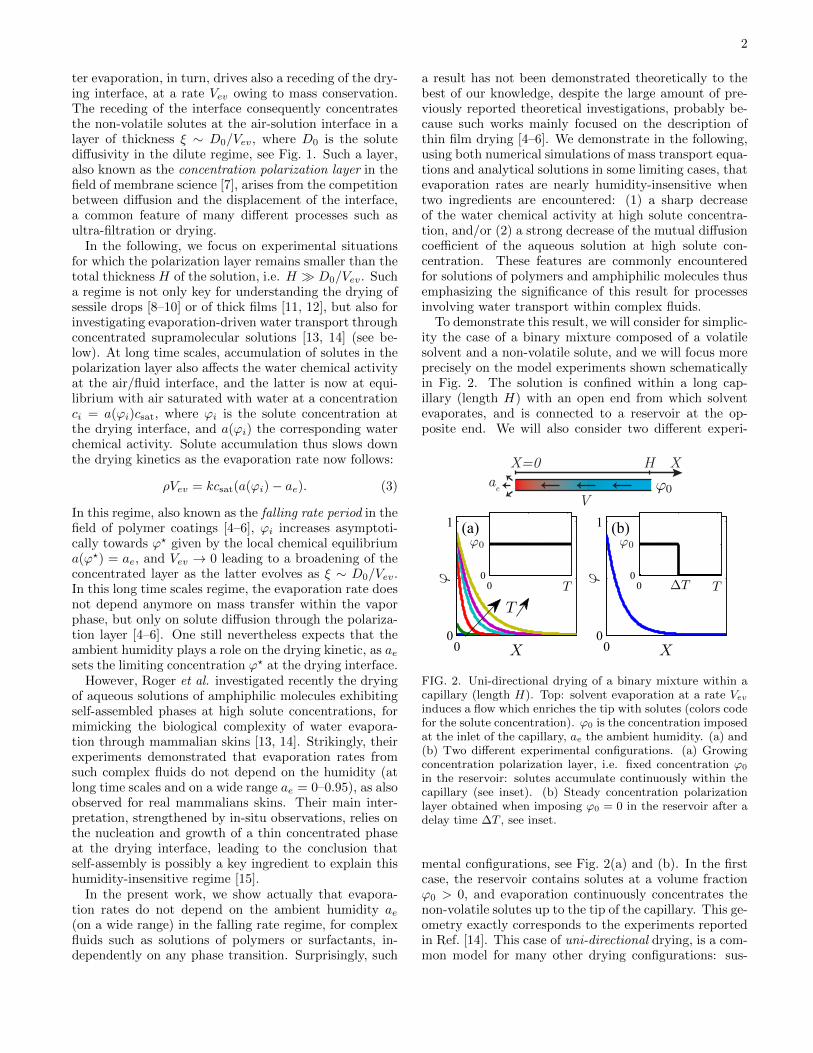
We first consider the most general case correspondingto non-constant a(ϕ) and D(ϕ), and given by the empir-ical formulae (16–18) displayed in Fig. 3. We solved thenon-linear equation Eq. (19) with v = a(ϕi)− ae for sev-eral humidities ae, and for several ψ values, see appendixB for details. We will consider ψ � 1 leading to evapo-

0 2000

1

x

ϕ

(a) (b)

0 0.01 0.02

0.7

0.8

0.9

1

0 0.25 0.75 10

300

400

−(∂ xϕ) x

=0

ae0

0.25

0.75

1

ϕi

FIG. 4. Steady polarization layer: non-constant a(ϕ) and

non-constant D(ϕ). (a) Steady profiles ϕ(x) for ψ = 15 andseveral ambient humidity ae (0: cyan; 0.2: blue; 0.4: red; 0.6:black; 0.8: green; 0.9: magenta). Insert: same data but at lowx. (b) Concentration gradient at the interface −(∂xϕ(x))x=0

vs. ae (◦, left axis), and concentration at the interface ϕi vs.ae (�, right axis), for ψ = 15. The solid line is the theoreticalcurve ϕ? vs. ae with a(ϕ?) = ae.

ration rates v � 1, owing to the significant decrease ofthe chemical activity at the drying interface. As shownin Fig. 4(a) for the case ψ = 15, the profiles almost col-lapse on a single curve for ambient humidities ae ≤ 0.9except in a narrow region of small x as shown in the in-set. The data shown in Fig. 4(b), −(∂xϕ)x=0 vs. ae, helpto reveal the strong concentration gradient at the inter-face for ae → 0 (over 4 decades for ae ranging from 0.95to 0). Fig. 4(b) also shows that the concentration at theinterface ϕi is close to ϕ? given by a(ϕ?) = ae, indicatingthus that the evaporation rates are indeed small for suchlarge ψ value.

The corresponding evaporation rates v are shownagainst the ambient humidity ae in Fig. 5(a) for ψ = 15.As pointed out in the introduction, the evaporation ratesare nearly constant over a wide range of ae (relative de-crease ' 2% for ae = 0–0.9, ψ = 15). Fig. 5(b) also showsthe calculated evaporation rates v for ae = 0, vs. 1/ψ.These data show that for ψ > 1, evaporation rates arevery well-fitted by v ' ϕc/ψ with ϕc = 0.48, suggestingpossibly that simple analytical expressions can be foundto explain why evaporation rates are insensitive to ae.

With real units, the evaporation rate follows Vev 'D0ϕc/Ψ independently of the humidity (Ψ being the di-mensionalized volume of solutes trapped in the capillary)

0 10

0.02

0.06

0.08

ae

v

(a)

0 30

1

1/ψ

v

(b)

FIG. 5. (a) Steady evaporation rate v vs. ae. � : case D(ϕ)given by Eq. (16) for ψ = 15, see also the correspondingprofiles in Fig. 4. The thick dark line is v = ϕc/ψ with ϕc =

0.48. �: case D(ϕ) = 1 for ψ = 15. The solid line is thetheoretical prediction v = ϕ?/ψ with a(ϕ?) = ae. The dashedline is the case expected for a pure solvent i.e. v = 1−ae. (b)

Steady evaporation rate v at ae = 0 vs. 1/ψ for the case D(ϕ)given by Eq. (16). The solid line is the best fit by v = ϕc/ψwith ϕc = 0.48.

and of the transport in the vapor phase (term J). Waterevaporation however still depends on diffusion in the liq-uid phase (term D0) and as shown later, the exact valueϕc accounts for the specific shape of D(ϕ).

We unveil below the role played by both D(ϕ) and a(ϕ)on the very small dependence of v with ae, using analyt-ical solutions obtained for simple expressions of D(ϕ).

B. Role of the activity only: case D(ϕ) = 1

In this case, concentration profiles are easily calculatedfrom Eq. (19) with the constraint given by Eq. (20), lead-ing to the exponential decay:

ϕ(x) = ψv exp(−vx) . (21)

For ψ � 1, one should have v � 1 to get a finite con-centration at the interface, and thus ϕi = ψv ' ϕ? withϕ? given by a(ϕ?) = ae. In that regime, the evaporationrate thus follows

v ' ϕ?

ψ, (22)

(Vev ' D0ϕ?/Ψ with real units). The water/PVA case is

shown in Fig. 5(a) for ψ = 15 and assuming D(ϕ) = 1.Symbols are the direct solutions of ψv = ϕi with Eq. (12)and the solid line is the theoretical approximation (22).With the assumption of a constant mutual diffusion co-efficient, evaporation rates are weakly sensitive to thehumidity variations (relative variations of < 20% overae = 0–0.8 for ψ = 15).

Indeed, a sharp decrease of the chemical activity athigh solute concentrations (see Fig. 3(a)) leads to ϕ? '1 over a large humidity range (see Fig. 4(b)). A weakdependance of the evaporation rate follows, because ofEq. (22). Nevertheless, the results reported in Fig. 5 show

6

that the variations of D with ϕ are key to understand theextremely small variations of the evaporation rate alongwith ae.

C. Role of the mutual diffusion coefficient:non-constant a(ϕ) and piecewise constant D(ϕ)

To capture the role played by the variation of the mu-tual diffusion coefficient with the solute concentration,we solve analytically the steady case Eq. (19) using a

piecewise constant function for D(ϕ). More precisely, wechose:

D(ϕ) = 1 for ϕ < ϕc

D(ϕ) = d for ϕ > ϕc

}(23)

with d < 1, as shown in the inset of Fig. 3(b). We alsoconsider humidities ae < a(ϕc) and large ψ values forwhich the concentration at the drying interface reachesϕi > ϕc. Integration of Eq. (19) in this simple configu-ration leads to the following concentration profile:

ϕ(x) = ϕi exp(−vx/d) for x < xc , (24)

ϕ(x) = ϕc exp(−v(x− xc)) for x > xc . (25)

The concentration field continuity imposes xc =(d/v) log(ϕi/ϕc). Integrating Eqs. (24-25) from x = 0to infinity and using the definition of ψ (Eq. (20)) yields:

v =ϕc + d(ϕi − ϕc)

ψ. (26)

In the general case, ϕi and v are obtained by solving nu-merically the set of algebraic equations (12,26). For largeψ, Eq. (12) can be replaced by ϕi ' ϕ?, and Eq. (26) di-rectly gives the evaporation rate v. As expected, Eq. (22)is recovered for d = 1. For d� 1, Eq. (26) reduces to:

v ' ϕcψ, (27)

where v no longer depends on ϕ?. We show in the follow-ing that this crude model based on a piecewise constantD(ϕ) can be used to explain most of the features of moregeneral cases.

The case d → 0 corresponds to the existence closeto the drying interface of a layer of vanishing thicknessxc ' (d/v) log(ϕ?/ϕc) with a diverging concentrationgradient at the interface: (∂xϕ)x=0 ' −ϕ?v/d, fromEq. (24). For larger x values, i.e. x > xc, concentrationprofiles collapse on a master curve, whatever the value ofthe humidity, with a smaller concentration gradient ona scale 1/v � xc, see Eq. (25). These behaviors werealso observed for the PVA case studied in section III A(Fig. 4). Furthermore, an equivalence between the sim-plified model and this more realistic case can be foundby fitting ϕc in Eq. (27) from the curve v vs. 1/ψ ofFig. 5(b) (PVA case with ae = 0). We get ϕc ' 0.48.For the PVA case, this specific value corresponds approx-imately to the concentration below which all the profiles

collapse at large x, whatever the value of the humidityae, see Fig. 4(a).

We can now draw a simple picture to explain why evap-oration rates are nearly insensitive to variations of ae inthis steady configuration. Concentrations at the inter-face reach ϕi ' ϕ? for ψ � 1, and the profiles displaystrong concentration gradients at the interface, owing tothe very small mutual diffusion coefficient. Concentra-tions thus drop from ϕ? to values ϕ ≤ ϕc on a very thinlayer (0–xc), and the contribution of this strong gradientto the total amount of solutes trapped within the capil-lary is negligible, see Eq. (20). The value of the ambienthumidity only plays a role on this thin layer throughϕ? and xc. For the remaining part of the profile (i.e.x ≥ xc), mutual diffusion coefficient is almost constant(D0 with real units in the simple model). Concentrationprofiles in this region are solutions of a diffusion problemwith constant diffusivity and concentration ϕc imposedat x = xc. When xc is very small, this is almost equiv-alent to imposing ϕc at x = 0. The effect of humiditythen drops out, because ϕc is a material property, henceindependent of ambient conditions.

Practically, vanishing diffusivity (d→ 0) is not strictlyrequired to get evaporation rates nearly insensitive to am-bient humidity. Indeed, assuming for instance d = 0.1,ϕc = 0.5 and ϕi ' ϕ? (as expected for large ψ) inEq. (26), v only decreases of ' 3% over ae = 0–0.8. Thisweak variation comes indeed from two superimposed ef-fects: (i) the small variation of the concentration at theinterface ϕi along with the humidity (due to the sharpvariation of a(ϕ) vs. ϕ at high solute concentration),and (ii) a small mutual diffusion coefficient at high so-lute concentration (presence of a thin layer with a highconcentration gradient at the drying interface).

IV. GROWING POLARIZATION LAYER (ϕ0 > 0)

We now turn to the time-dependent case describedschematically in Fig. 2(a). In this regime, concentra-tion in the reservoir is ϕ0 � 1, and solutes continu-ously accumulate within the capillary. At early stages,the drying-induced flow convects solutes at the tip ofthe capillary where they accumulate in a region of sizeξ ∼ 1 (ξ ∼ D0/Vev with real units). At longer time scaleshowever, concentration at the tip is expected to increaseasymptotically towards ϕ?, given by a(ϕ?) = ae, leadingto a slowing down of the evaporation rate (because ofEq. (12)), and thus of the convective flux −(ϕv). Onethus expects a broadening of the concentrated layer asthe latter evolves as ξ ∼ D0/Vev, and we will mainly fo-cus in the following on this long-time scales regime. Noteagain that the assumption of a semi-infinite medium, i.e.H � D0/Vev see above, imposes a limiting time scalesfor our description which depends on H, as the evap-oration rate Vev is expected to slow down continuouslyat long time scales. Note also that this time-dependentcase is strictly analogous to the drying of quiescent thick

7

films, as for instance studied in Ref. [28]. One can in-deed show using an appropriate change of variables, thatEqs. (11–12) along with the boundary and initial con-ditions (13–15) corresponds to the modeling of solventevaporation from a thick film, see appendix A.

A. General case: non-constant a(ϕ) and

non-constant D(ϕ)

0 500 10000

1

t

x

ϕ

(a) (b)

ϕ⋆

0 10

ϕ⋆

x/√t

ϕ

0

100

−(∂ xϕ) x

=0

100

102

104

0

ϕi

t

FIG. 6. Growing polarization layer: non-constant a(ϕ) and

non-constant D(ϕ). (a): ϕ(x) vs. x for several times t = 103;104, 105 and 106 (ae = 0.4, ϕ0 = 0.01) for the water/PVAcase. The inset displays the same data rescaled against x/

√t,

ϕ? is given by a(ϕ?) = 0.4. (b) Concentration gradient at theinterface −(∂xϕ(x))x=0 vs. t (left axis), and concentration atthe interface ϕi vs. t (right axis)

We used a commercial finite elements software, Com-sol Multiphysics, to solve numerically the transportequations (11–12) with the boundary and initial condi-tions (13–15), assuming the empirical formulae (16–18)

for a(ϕ) and D(ϕ) (see Fig. 3). Comsol Multiphysics isbased on the Galerkin method. We used quadratic La-grange elements and BDF solver.

Figure 6 displays some concentration profiles com-puted for ae = 0.4 and ϕ0 = 0.01 at long time scales(t > 1000). In this time-dependant case, concentrationreaches ϕi ' ϕ? given by a(ϕ?) = ae for t > 1000. Con-centration profiles then widen over time, and again withsteep concentration gradients at the interface (which ulti-mately decrease owing to the decrease of the evaporationrate). Concentration profiles almost collapse on a singlecurve when plotted against x/

√t suggesting that a self-

similar profile approximates the calculated solutions inthis long-time scale regime.

The corresponding temporal evolution of the evapora-tion rate v is shown in Fig. 7(a) for various humidities.At early stages, v ' 1−ae as the solute concentration atthe interface does not modify strongly the water chemicalactivity (the so-called constant rate regime). At longertime scales, evaporation rates collapse on a master curveregardless of the value of the humidity. In this asymp-

100

105

0

1

t

v

(a)

0 6−3

0

log10 t

log 1

0v

100

105

0

1

t

v

(b)

0 6−3

0

log10 t

log 1

0v

FIG. 7. Evaporation rate v vs. t for several ambient humidi-ties ae (0: cyan; 0.2: blue; 0.4: red; 0.6: black; 0.8: green).

(a) water/PVA general case, (b) case D(ϕ) = 1. The circlesare simple estimates of the onset of the falling rate period as-suming constant D(ϕ) and v = 1−ae at early time scales, seetext and appendix C for details. The insets display the samedata in a log-log plot. The black lines show the behaviorsv ∼ 1/

√t.

totic regime, the log-log plot in Fig. 7(a) helps to revealthat the evaporation rate decreases as

v ' α√t, (28)

as also reported by Roger et al. for water/surfactantsolutions, in an experimental configuration close to theone studied here [14].

0 0.2 0.4 0.6 0.8 10

2

4

6

8

ae

Prefactor

α,seeEq.(28)

FIG. 8. Prefactor α vs. ambient humidities ae. α is esti-mated from the evaporation rate in the asymptotic regimeusing Eq. (28), i.e. v ' α/

√t; ◦: water/PVA case, �:

case D(ϕ) = 1. The thin line is the theoretical predictionEq. (30). The thick line is the prediction given by Eq. (32)with ϕc ' 0.48.

Figure 8 displays the prefactor α fitted from the datav vs. t at long time scales using Eq. (28), and against ae.

8

α is extremely insensitive to the variations of ae (varia-tions below < 0.1% over the range ae = 0–0.9) suggestingagain that humidity does not play any role (at long timescales) on the evaporation kinetics, even in this time-dependent configuration. To unveil again the role playedby both the shape of the solvent chemical activity a(ϕ)

and that of the mutual diffusion coefficient D(ϕ), we turn

to simple expressions of D(ϕ).

B. Role of the activity only: case D(ϕ) = 1

To emphasize the role played by the activity only, wesolved Eqs. (11–12) with the boundary and initial condi-

tions (13–15), but assuming D(ϕ) = 1.

0 5000

1

t

x

ϕ

(a) (b)

ϕ⋆

00

ϕ⋆

x/√t

ϕ

0

1

−(∂ xϕ) x

=0

100

102

104

0

ϕi

t

FIG. 9. Growing polarization layer: non-constant a(ϕ) and

D(ϕ) = 1. (a): ϕ(x) vs. x for several times t = 103; 7.9×103,6.3×104 and 5×105 (ae = 0.4, ϕ0 = 0.01. The inset displaysthe same data rescaled against x/

√t, ϕ? is given by a(ϕ?) =

0.4. (b) Concentration gradient at the interface −(∂xϕ(x))x=0

vs. t (left axis), and concentration at the interface ϕi vs. t(right axis)

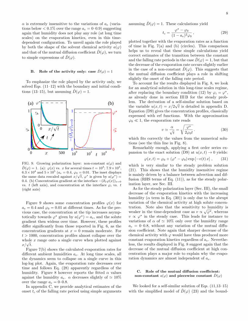
Figure 9 shows some concentration profiles ϕ(x) forae = 0.4 and ϕ0 = 0.01 at different times. As for the pre-vious case, the concentration at the tip increases asymp-totically towards ϕ? given by a(ϕ?) = ae, and the solutegradient then widens over time. However, these profilesdiffer significantly from those reported in Fig. 6, as theconcentration gradients at x = 0 remain moderate. Fort > 1000, concentration profiles almost collapse over thewhole x range onto a single curve when plotted againstx/√t.

Figure 7(b) shows the calculated evaporation rates fordifferent ambient humidities ae. At long time scales, allthe dynamics seem to collapse on a single curve in thislog-log plot. Again, the evaporation rate decreases overtime and follows Eq. (28) apparently regardless of thehumidity. Figure 8 however reports the fitted α valuesagainst the humidity ae. α decreases slightly of ' 10%over the range ae = 0–0.8.

In appendix C, we provide analytical estimates of theonset tc of the falling rate period using simple arguments

assuming D(ϕ) = 1. These calculations yield

tc =ϕ? − ϕ0

(1− ae)2ϕ0, (29)

plotted together with the evaporation rates as a functionof time in Fig. 7(a) and (b) (circles). This comparisonhelps us to reveal that these simple calculations yieldcorrect estimates of the transition between the constantand the falling rate periods in the case D(ϕ) = 1, but thatthe decrease of the evaporation rate occurs slightly earlierin the case of a non-constant D(ϕ). This suggests thatthe mutual diffusion coefficient plays a role in shiftingslightly the onset of the falling rate period.

To account for the results displayed in Fig. 8, we lookfor an analytical solution in this long-time scales regime,after replacing the boundary condition (12) by ϕi = ϕ?,as already done in section III B for the steady prob-lem. The derivation of a self-similar solution based onthe variable u(x, t) = x/2

√t is detailed in appendix D.

Equation (D9) gives the concentration profiles, classicallyexpressed with erf functions. With the approximationϕ0 � 1, the evaporation rate reads

v ' α√t

=

√ϕ?

2ϕ0t. (30)

which fits correctly the values from the numerical solu-tions (see the thin line in Fig. 8).

Remarkably enough, applying a first order series ex-pansion to the exact solution (D9) at u(x, t)→ 0 yields:

ϕ(x, t) = ϕ0 + (ϕ? − ϕ0) exp [−v(t)x] , (31)

which is very similar to the steady problem solution(21). This shows that the humidity insensitive regimeis mainly driven by a balance between advection and dif-fusion (RHS terms of Eq. (11)), as for the steady polar-ization layer, see Sec. III.

As for the steady polarization layer (Sec. III), the smalldecrease of the evaporation kinetics with the increasinghumidity (α term in Eq. (30)) is only due to the abruptvariation of the chemical activity at high solute concen-tration. Note also that the sensitivity to humidity isweaker in the time-dependent case as v ∝ √ϕ?, whereasv ∝ ϕ? in the steady case. This leads for instance tovariations of α of ' 10% only over the humidity rangeae = 0–0.8, without any variation of the mutual diffu-sion coefficient. Note again that sharper decrease of thechemical activity with ϕ would have thus produced moreconstant evaporation kinetics regardless of ae. Neverthe-less, the results displayed in Fig. 8 suggest again that thedecrease of the mutual diffusion coefficient at high con-centration plays a major role to explain why the evapo-ration dynamics are almost independent of ae.

C. Role of the mutual diffusion coefficient:non-constant a(ϕ) and piecewise constant D(ϕ)

We looked for a self-similar solution of Eqs. (11,13–15)

with the simplified model of D(ϕ) (23) and the bound-

9

ary condition ϕi = ϕ?. The derivation is detailed inappendix D. With the assumptions ϕ0 � 1 and d � 1,the evaporation rate reads:

v '√

ϕc2ϕ0t

. (32)

This simple prediction looks like Eq. (30) with the sub-stitution ϕ? → ϕc. Figure 8 compares this theoreticalprediction with the numerical results, using the valueϕc ' 0.48 derived from the steady polarization layer in-vestigated in Sec. III C, and demonstrates that the agree-ment is very good.

The evaporation rate Eq. (32) corresponds to the solu-tion of a diffusion problem with a constant diffusivity andthe concentration ϕc imposed at the drying interface. Asfor the steady polarization layer, the major part of theliquid phase is shielded from the gas phase by a thin layerof liquid with a large concentration gradient. We there-fore conclude that the same mechanisms are acting inboth steady and growing polarization layer.

V. CONCLUSIONS AND DISCUSSIONS

In the present paper, we have investigated theoreticallythe one-dimensional water transport induced by evapo-ration from a molecular mixture. At long time scales,solute concentration at the drying interface tends to itsequilibrium value, i.e. ϕi → ϕ?, and the evaporationdriving force asymptotically drops to zero. In this regime,evaporation rates are small and the overall water trans-port is mainly dominated by diffusion within the liquidphase, as already known. In this paper we show that,for some complex fluids, evaporation rates are humidity-insensitive in a wide range of humidity, unlike expected.

This result comes from two superimposed effects.First, the sharp decrease of the water chemical activ-ity at high concentrations (as observed for instance forpolymer solutions) leads to small variations of ϕ? alongwith ae, and thus to small variations of the correspondingevaporation rate. This feature is specific to the case ofmolecular mixtures only, and we do not expect similar ob-servations for colloidal dispersions for instance. Indeed,uni-directional drying of dispersions may also induce theformation of (porous) non-volatile aggregates at the dry-ing interface, but they do not not in turn affect the chem-ical activity of the solvent, and hence evaporation rates,see e.g. [29–31]. In the case of molecular binary mix-tures, the decrease of the mutual diffusion coefficient ofthe mixture at high concentration is key to explain whyevaporation rates are remarkably independent of ae overa wide humidity range, see for instance Fig. 8. The basicmechanism is the following. The strong decrease of D(ϕ)induces a steep concentration gradient at the drying in-terface. The concentration profile thus reaches values forwhich the mutual diffusion becomes again close to D0, atpositions x close to the drying interface (ϕ = ϕc at x = xc

in our model with a piecewise constant D(ϕ)). The re-maining part of the profile, which contributes mainly tothe value of the evaporation rate, is therefore shieldedfrom the humidity variations which only play a role onthis thin layer. This is the key interpretation providedby Roger et al. in the context of water transport throughself-assembled concentrated phases to explain why evap-oration rates are insensitive to ae [14]. Surprisingly, de-spite (i) an extensive survey of the abundant literatureconcerning notably the drying of polymeric films, and (ii)the simplicity of the above theoretical description, such aregime has never been discussed theoretically to the bestof our knowledge.

Note that Roger et al. used the concept of permeabilityinstead of mutual diffusion to interpret their result. Mu-tual diffusion actually results from an interplay between athermodynamic factor taking into account the variationof the chemical activity along with the concentration,and a mobility factor related to the relative transport so-lutes/solvent [32]. In the context of molecular mixtures,D(ϕ) is often written as:

D(ϕ) = −M(ϕ)∂ ln a(ϕ)

∂ϕ, (33)

where M(ϕ) is a mobility factor, which takes for instancethe following form in the field of colloidal dispersions:

M(ϕ) = −ϕkη

kBT

vm, (34)

where k is the water permeability through the colloidaldispersion, η the water viscosity, T the absolute tem-perature, and vm the molecular volume of water, seee.g. Ref. [33]. For self-assembled phases of surfactants,permeability (or equivalently the mobility factor) maydecrease strongly within a phase owing to its specific tex-ture [34]. This may thus lead to the conclusion that thehumidity-insensitive evaporation-driven water transportis related to self-assembly. However, we showed in thepresent work that such a regime is also expected for anybinary mixture, independently of any phase transition,when its mutual diffusion coefficient decreases at highconcentration. Note finally that the decrease of D(ϕ)may not be extremely strong, as a sharp decrease of thewater chemical activity also contributes significantly tothis effect.

In the model investigated above, we have assumed lo-cal thermodynamic equilibrium conditions. Our modelmay thus apply to a wide range of experimental situ-ations including for instance the drying of polymer so-lutions when no evaporation-induced glass transition oc-curs, or water transport through self-assembled phases ofsurfactants (without including the nucleation and growthsteps of the latter). However our model, and particu-larly the steady configuration shown in Fig. 2(b), mayalso apply to some extent to the description of one di-mensional drying-induced water transport through cross-linked dilute hydrogels. One can indeed derive similar

10

equations providing elastic contributions to the waterchemical activity and to the mutual diffusion coefficientare negligible, disregarding non-Fickian mass transport,and taking into account properly the one dimensionalswelling of the network, see for instance Ref. [19], andalso Refs. [11, 12, 35] for some investigations of the gen-eral case. We hope in a near future to investigate suchan issue in more details, and particularly the role of thehumidity. For non-negligible elastic contributions for in-stance, the phenomenology described above, particularlyin Fig. 2, may not apply, as elastic effects may inducethe growth of a (permeable) gel phase at a critical con-centration [11, 12]. We hope as a research perspectiveto evaluate the significance of these elastic effects withrespect to the mechanisms unveiled above. Such exper-imental cases may indeed be relevant for a wide rangeof experimental situations including for instance drying-induced water transport through biomaterials or throughsoft contact lenses [20].

Appendix A: Unidirectional drying vs. thick filmdrying

We consider the 1D drying of a motionless thick liquidfilm. The liquid gas interface initially stands at heightY = 0, then decreases due to the volume loss induced byevaporation, see Fig. 10. The solvent global mass balance

ae

Y

,X=0

0 10

1

ϕ0

a(ϕ)

(a)

0 110−15

10−10

ϕ

D(ϕ)(m

2/s)

(b)

0 1

1

d

ϕc

D(ϕ

)

X

Y=Yi

Y=0

FIG. 10. Schematic view of the drying of a quiescent thickfilm.

reads:

dYidT

= J(a(ϕi)− ae) , (A1)

where Yi is the interface position, and ϕi the solute con-centration at the interface. Within the volume, the solutevolume fraction verifies:

∂Tϕ = ∂Y (D(ϕ)∂Y ϕ) for Y > Yi . (A2)

We use the dimensionless units defined in Eq. (10) to getthe following equations:

dyidt

= a(ϕi)− ae , (A3)

∂tϕ = ∂y(D(ϕ)∂yϕ) for y > yi . (A4)

Considering the motion of the liquid-gas interface at avelocity dyi/dt, the non-volatility of the solute resultsin:

ϕidyidt

+ (D(ϕ)∂yϕ)y=yi = 0 . (A5)

Assuming that the liquid film is thick enough to beconsidered as a semi-infinite medium yields the secondboundary condition:

ϕ(y →∞, t) = ϕ0. (A6)

The initial condition is:

ϕ(y, t = 0) = ϕ0 for y > 0. (A7)

One recovers strictly Eqs. (11–15) from the above modeldescribing the drying of a quiescent thick film by usingthe change of variable:

x = y(x, t)− yi(t) , (A8)

and with the relation v = dyi/dt. These two problemsare thus strictly equivalent.

Appendix B: Numerical resolution of Eq. (19)

Our aim is to compute the solution of Eq. (19) for afixed ψ value given by Eq. (20), and with v given byEq. (12). We proceeded as follows. We used the solverode113 (Matlab) to compute the solutions of the firstorder ordinary differential equation Eq. (19) for a givenhumidity ae, and for many different boundary conditionsϕ(x = 0) increasing in a logarithmic way from ϕj=1 =ϕ? − 0.5 to ϕj=N = ϕ? − ε with ε = 10−5 and N = 100typically. To describe correctly the strong concentrationgradient at the interface, each solution is calculated on alogarithmic x scale.

For each solution with boundary condition ϕ(x = 0) =ϕj , we then calculate the total amount of solute ψj us-ing Eq. (20). The relation ψj vs. ϕj allows us to esti-mate precisely using a linear interpolation, the boundarycondition ϕ(x = 0) which leads to a given ψ value, e.g.ψ = 15 for the cases shown in Fig. 4.

Appendix C: Simple estimates of the onset of thefalling rate period

Our first aim is to derive an analytical approximation,at early time scales, of the solutions of Eqs. (11-12) withboundary conditions given by Eqs. (13-14) and initialcondition Eq. (15).

At early stages, concentration profiles follow ϕ(x, t)�ϕ?, a(ϕ) ' 1, D(ϕ) ' 1, and the evaporation rate givenby Eq. (12) is nearly constant, v ' 1 − ae. The 1Dtransport equation Eq. (11) can be thus written as

∂tϕ = −∂xj , (C1)

11

with the non-dimensionalized solute flux j = −(1−ae)ϕ−∂xϕx. Using Eq. (C1), it is straightforward to demon-strate that the flux follows in turn

∂tj = (1− ae)∂xj + ∂2xj . (C2)

After a transient, the concentration process tends toan asymptotic regime for which the flux is stationary∂tj = 0, still assuming a dilute solution ϕ(x, t) � ϕ?.This steady flux can be estimated using Eq. (C2) andthe boundary conditions Eqs. (13-14) which simply readj(x = 0) = 0 and j(x� 1) = −ϕ0(1−ae), leading finallyto

j(x) = −ϕ0(1− ae) (1− exp [−(1− ae)x]) . (C3)

In this asymptotic regime, the rate of concentrationgiven by Eq. (C1) follows approximatively

∂tϕ ' ϕ0(1− ae)2 exp (−(1− ae)x) , (C4)

and the concentration profiles are thus well-approximated by

ϕ(x, t) ' ϕ0 + t ϕ0(1− ae)2 exp (−(1− ae)x) , (C5)

using the initial condition Eq. (15). The onset of thefalling rate period can be estimated by ϕ(x = 0, tc) = ϕ?

using the previous relation, leading to:

tc =ϕ? − ϕ0

(1− ae)2ϕ0, (C6)

see the circles shown in Fig. 7.

Appendix D: Self-similar solutions

We use the model of evaporation from a thick film de-scribed in apprendix A to find a self-similar solution inthe long-time scale regime. Eq. (A3) is replaced by thefollowing Dirichlet boundary condition:

ϕ(yi, t) = ϕ? , (D1)

where ϕ? is a constant given by a(ϕ?) = ae. This is fullyjustified as dyi/dt→ 0 in the long time scale regime (seeEq. A3). Equations (A4–A6) and (D1) are rewritten as-suming that the solute volume fraction ϕ(y, t) dependson a single variable u(y, t). As done classically for dif-fusion problems, we choose u(y, t) = y/(2

√t) [36]. The

partial derivatives equation (A4) turns to the ordinarydifferential equation:

d

du

[D(ϕ)

dϕ

du

]+ 2u

dϕ

du= 0 for u > ui (D2)

where ui = yi//(2√t). Equations (A6) and (A7) collapse

onto a single boundary condition:

ϕ(u→∞) = ϕ0. (D3)

The Dirichlet condition (D1) now reads:

ϕ(ui) = ϕ? . (D4)

As ϕ? is a constant, a necessary condition for the self-similar solution to exist is ui = α where α is a constant tobe determined. Immediate consequences of this conditionare:

yi = 2α√t and

dyidt

=α√t. (D5)

The boundary condition Eq. (A5) along with Eq. (D5)yields:

2αϕi + D(ϕi)dϕ

du(u = α) = 0 , (D6)

whose unknown is α. The self-similar solution exists ifEq. (D6) has a solution.

1. Constant mutual diffusion coefficient D(ϕ) = 1

We solve Eqs. (D2–D4, D6) to find:

ϕ(u) = ϕ0 + (ϕ? − ϕ0)erfc(u)

erfc(α). (D7)

Injecting Eq. (D7) into (D6) yields:

ϕ? − ϕ0

ϕ?=√π α erfc(α) exp(α2) , (D8)

hence leading to α.To recover the solution for the problem of unidirec-

tional drying, we now use the change of variable (A8)and we define u(x, t) = x/(2

√t). The self-similar solu-

tion is now:

ϕ(u) = ϕ0 + (ϕ? − ϕ0)erfc(u+ α)

erfc(α), (D9)

and Eq. (D8) is unchanged. With the assumption ϕ0 �ϕ?, a simple approximate solution of Eq. (D8) is obtainedby a second order series expansion of erfc at α→∞. Weget:

α '√

ϕ?

2ϕ0, (D10)

where the evaporation rate follows:

v =

√ϕ?

2ϕ0t. (D11)

2. Piecewise constant mutual diffusion coefficientD(ϕ)

We consider now a piecewise constant diffusion coef-ficient, falling from 1 to a constant value d at a solutevolume fraction ϕc, see Eq. (23) and Fig. 3(b). We defineyc the abscissa such that ϕ(yc, t) = ϕc. With the changeof variable u(y, t) = y/(2

√t), the solute volume fraction

ϕ(u) verifies Eq. (D2) with D(ϕ) = d for ui < u < uc,

and D(ϕ) = 1 for uc < u, where ui = yi/(2√t) and

12

uc = yc/(2√t). The existence of a self-similar solution re-

quires yi = 2α√t and yc = 2β

√t, where α and β are two

constants to be determined. Boundary conditions (D3–D4) are supplemented with flux conservation equationsat u = ui = α and u = uc = β:

2αϕ∗ + ddϕ

du(u = α) = 0, (D12)

ddϕ

du(u = β−) =

dϕ

du(u = β+). (D13)

The solution is

ϕ(u) = (ϕ∗ − ϕc)erfc( u√

d)− erfc( α√

d)

erfc( α√d)− erfc( β√

d)

+ ϕ∗ , (D14)

for ui < u < uc, and

ϕ(u) = (ϕc − ϕ0)erfc(u)

erfc(β)+ ϕ0 , (D15)

for uc < u. Injecting Eqs. (D14–D15) in Eqs. (D12–D13)provides two equations to be solved to get α and β:√

π

d

[erfc(

α√d

)− erfc(β√d

)

]exp(

α2

d)α =

ϕ∗ − ϕcϕ∗

,

(D16)[erfc( α√

d)− erfc( β√

d)]

exp(β2

d )

erfc(β)√d exp (β2)

=ϕ∗ − ϕcϕc − ϕ0

. (D17)

Eqs. (D16–D17) can be solved numerically. However,we are particularly interested in the asymptotic case d→0, for which an analytical solution can be found. Withthe approximation erfc(z → ∞) ' exp(−z2)/(

√πz),

Eqs. (D16–D17) turn to:

α

βexp

(α2 − β2

d

)=ϕcϕ∗

, (D18)

√πβ erfc (β) exp (β2)

exp(β2−α2

d

)βα − 1

=ϕc − ϕ0

ϕ∗ − ϕc. (D19)

Because Eqs. (D18–D19) require non zeros left hand sidesto be satisfied, d → 0 implies β → α. Using Eq. (D18)to eliminate α in Eq. (D19) yields:

√π β erfc (β) exp (β2) =

ϕc − ϕ0

ϕc. (D20)

By analogy with Eq. (D8), and considering the assump-tion ϕ0 � ϕc, we get finally:

α ' β '√

ϕc2ϕ0

. (D21)

ACKNOWLEDGMENTS

The authors thank ANR EVAPEC (13-BS09-0010-01)for funding.

[1] A. S. Mujumdar. Handbook of Industrial Drying. CRCPress, 2014.

[2] B. R. Bird, E. W. Stewart, and E. N. Lightfoot. Transportphenomena. Wiley international edition, 2002.

[3] E. L. Cussler. Diffusion : Mass Transfer in Fluid Sys-tems. Cambridge University Press, 1997.

[4] R. Saure, G. R. Wagner, and E.-U. Schlunder. Drying ofsolvent-borne polymeric coatings. i. modeling the dryingprocess. Surf. Coat. Technol., 99:253, 1998.

[5] B. Guerrier, C. Bouchard, C. Allain, and C. Benard. Dry-ing kinetics of polymer films. AIChE, 44:791, 1998.

[6] M. Okazaki, K. Shioda, K. Masuda, and R. Toei. Dryingmechanism of coated film of polymer solution. JournalOf Chemical Engineering Of Japan, 7:99–105, 1974.

[7] G. Belfort, R.H. Davis, and A. L. Zydney. The behaviorof suspensions and macromolecular solutions in crossflow

microfiltration. J. Membrane Sci., 96:1–58, 1994.[8] T. Kajiya, E. Nishitani, T. Yamaue, and M. Doi. Piling-

to-buckling transition in the drying process of polymersolution drop on substrate having a large contact angle.Phys. Rev. E, 73:011601, 2006.

[9] L. Pauchard and C. Allain. Buckling instability inducedby polymer solution drying. Europhys. Lett., 62:897–903,2003.

[10] K.A. Baldwin, M. Granjard, D.I. Willmer, K. Sefi-ane, and D.J. Fairhurst. Drying and deposition ofpoly(ethylene oxide) droplets determined by peclet num-ber. Soft Matter, 7:7819, 2011.

[11] T. Okuzono, K. Ozawa, and M. Doi. Simple model ofskin formation caused by solvent evaporation in polymersolutions. Phys. Rev. Lett., 97:136103–136106, 2006.

[12] T. Okuzono and M. Doi. Effects of elasticity on drying

13

processes of polymer solutions. Phys. Rev. E, 77:030501–030504, 2008.

[13] E. Spaar and H. Wennerstrom. Diffusion through a re-sponding lamellar liquid crystal: a model of moleculartransport across stratum corneum. Colloids and SurfacesB: Biointerfaces, 19:103–116, 2000.

[14] K. Roger, M. Liebi, J. Heimdal, Q.D. Pham, andE. Spaar. Controlling water evaporation through self-assembly. Proc. Natl. Acad. Sci. USA, 113:10275–10280,2016.

[15] A. H. Trabesinger. Worth all the sweat. Nature Physics,320:340–342, 1986.

[16] D. Brutin, editor. Droplet Wetting and Evaporation.From Pure to Complex Fluids. Academic Press, Elsevier,2015.

[17] L. Daubersies and J.-B. Salmon. Evaporation of solutionsand colloidal dispersions in confined droplets. Phys. Rev.E, 84:031406, 2011.

[18] L. Daubersies, J. Leng, and J.-B. Salmon. Steady andout-of-equilibrium phase diagram of a complex fluid atthe nanolitre scale: combining microevaporation, confo-cal raman imaging and small angle x-ray scattering. LabChip, 13:910–919, 2013.

[19] S. Jeck, P. Scharfer, W. Schabel, and M. Kind. Wa-ter sorption in poly(vinyl alcohol) membranes: An ex-perimental and numerical study of solvent diffusion in acrosslinked polymer. Chemical Engineering and Process-ing, 50:543–550, 2011.

[20] F. Fornasiero, D. Tanga, A. Boushehri, John Praus-nitz, and C. J. Radke. Water diffusion through hydro-gel membranes. a novel evaporation cell free of externalmass-transfer resistance. Journal of Membrane Science,320:423–430, 2008.

[21] P. G. de Gennes. Solvent evaporation of spin cast films:rusteffects. Eur. Phys. J. E, 7:31–35, 2002.

[22] M. Schindler and A. Ajdari. Modeling phase behaviorfor quantifying micro-pervaporation experiments. Eur.Phys. J E, 28:27–45, 2009.

[23] P. Neogi. Diffusion in polymers. CRC Press, 1996.[24] P.J. Flory. Principles of Polymer Chemistry. Cornell

University Press, Ithaca, New-York, 1973.[25] P.-G. de Gennes. Scaling Concepts in Polymer Physics.

Cornell University Press, Ithaca, 1979.[26] Z. Gu and P. Alexandridis. Drying of films formed by or-

dered poly(ethylene oxide) -poly(propylene oxide) blockcopolymer gels. Langmuir, 21:1806, 2005.

[27] F. Doumenc and B. Guerrier. Mutual diffusion coeffi-cient and vapor-liquid equilibrium data for the systempolyisobutylene + toluene. J. Chem. Eng. Data, 50:983–988, 2005.

[28] F. Doumenc, B. Guerrier, and C. Allain. Proc. of 40thInternational Symposium on Macromolecules MACRO2004, Paris,, 2004.

[29] P. Lidon and J.-B. Salmon. Dynamics of unidirectionaldrying of colloidal dispersions. Soft Matter, 10:4151–4161, 2014.

[30] L. A. Brown, C. F. Zukoski, and L. R. White. Consoli-dation during drying of aggregated suspensions. AIChE,48:492, 2002.

[31] R. W. Style and S. S. Peppin. Crust formation in dryingcolloidal suspensions. Proc. R. Soc. A, 467:174–193, 2011.

[32] S. R. De Groot and P. Mazur. Non-Equilibrium Thermo-dynamics. Dover Publications, 2013.

[33] S. S. Peppin, J. A. Elliott, and M. G. Worster. Pres-sure and relative motion in colloidal suspensions. Phys.Fluids, 17:053301–053309, 2005.

[34] E. Spaar and H. Wennerstrom. Responding phospholipidmembranesnterplay between hydration and permeability.Biophysical Journal, 81:1014–1028, 2001.

[35] T. Bertrand, J. Peixinho, S. Mukhopadhyay, and C. W.MacMinn. Dynamics of swelling and drying in a sphericalgel. Phys. Rev. Applied, 6:064010, 2016.

[36] J. Crank. The mathematics of diffusion. Oxford univer-sity press, 1975.