Combined study of evaporation from liquid surface by background orientedschlieren, infrared thermal imaging and numerical simulation

N.A. Vinnichenko1,a, A.V. Uvarov1, and Yu.Yu. Plaksina1

1Lomonosov Moscow State University, Faculty of Physics, 119991 Leninskiye Gory, 1/2, Moscow, Russia

Abstract. Temperature fields in evaporating liquids are measured by simultaneous use of Background OrientedSchlieren (BOS) technique for the side view and IR thermal imaging for the surface distribution. Good agree-ment between the two methods is obtained with typical measurement error less than 0.1 K. Two configurationsof surface layer are observed: thermocapillary convection state with moving liquid surface and small thermalcells, associated with Marangoni convection, and ”cool skin” with negligible velocity at the surface, larger cellsand dramatic increase of velocity within 0.1 mm layer beneath the surface. These configurations are shown to beformed in various liquids (water with various degrees of purification, ethanol, butanol, decane, kerosene, glyc-erine) depending rather on initial conditions and ambient parameters than on the liquid. Water, which has beenconsidered as the liquid without observable Marangoni convection, actually can exhibit both kinds of behaviorduring the same experimental run. Evaporation is also studied by means of numerical simulations. Separate prob-lems in air and liquid are considered, with thermal imaging data of surface temperature making the separationpossible. It is shown that evaporation rate can be predicted by numerical simulation of the air side with ap-propriate boundary conditions. Comparison is made with known empirical correlations for Sherwood-Rayleighrelationship. Numerical simulations of water-side problem reveal the issue of velocity boundary conditions atthe free surface, determining the structure of surface layer. Flow field similar to observed in the experiments isobtained with special boundary conditions of third kind, presenting a combination of no-slip and surface tensionboundary conditions.

1 Introduction

Evaporation at the free surface of liquid results in coolingof the surface and intensive heat exchange between bulkliquid and atmosphere. A thin surface layer is formed withtypical thickness about 1 mm, where temperature dropsabout 0.5 K. Depending on the conditions, different struc-tures can be observed at the surface and inside the sur-face layer, including Marangoni convection vortices, coldliquid filaments, motionless ”cool skin” and tops of Ray-leigh vortices. Despite its small thickness, it is this surfacelayer which determines the intensity of heat exchange be-tween liquid and atmosphere and evaporation rate. Thus,adequate experimental measurements and theoretical un-derstanding of its thermal structure are crucial for predict-ing evaporation rates and heat losses in numerous applica-tions involving evaporating liquids. Evaporation from wa-ter reservoirs, energy consumption of indoors swimmingpool facilities, cooling performance of air-conditioning sys-tems, technological drying processes, geophysical and en-vironmental aspects including life cycle of plankton – justto name a few. Satellite-based remote sensing of the oceantemperature also suffers from ambiguity associated withevaporation: surface temperature, which is actually mea-sured by infrared thermal imaging (IRTI), is different from

a e-mail:nickvinn@yandex.ru

the bulk temperature, and the difference is determined byevaporation rate.

Average vertical temperature profile below the liquidsurface can be approximated by simple exponential fit [1]:

T(z) = Tbulk + (Ts − Tbulk) exp(− zδ

), (1)

whereTs is the surface temperature of liquid,Tbulk is liquidtemperature far from the surface andz is the depth. Thisprofile is governed by two parameters: temperature drop∆T = Tbulk − Ts and surface layer thicknessδ. Major ex-perimental difficulties arise from the fact that (Tbulk − Ts)is usually of order 0.1 K andδ is about 1 mm. This sug-gests temperature gradients of several hundred K m−1 andthermal fluxes∼ 102 W m−2. There are two groups of ex-perimental techniques. Methods of the first group allowmeasuring average values forδ and∆T. Temperature dropcan be found e.g. by simultaneous thermocouple and IRTImeasurements [2], and layer thickness is estimated fromthe total heat flux. Total heat flux is interpreted as molecu-lar one

Qtotal = −λ dTdz

∣∣∣∣∣z=0

=∆Tδ. (2)

Thus, layer thickness can be found if the total heat flux isknown. In laboratory it can be determined from standardthermophysical measurements of liquid sample cooling, or

EPJ Web of ConferencesDOI: 10.1051/C© Owned by the authors, published by EDP Sciences, 2013

,epjconf 201/

01093 (2013)4534501093

This is an Open Access article distributed under the terms of the Creative Commons Attribution License 2 0 , which . permits unrestricted use, distributiand reproduction in any medium, provided the original work is properly cited.

on,

Article available at http://www.epj-conferences.org or http://dx.doi.org/10.1051/epjconf/20134501093

EPJ Web of Conferences

from evaporation rate. In natural conditions small contain-ers are immersed into water reservoir and evaporation rateis measured, or profiler thermoprobes of various types areused [1]. Bulk formulae, relating heat fluxes to temperatureand humidity values at various heights, have been elabo-rated both for laboratory [3] and in situ measurements [4].These relations allow finding estimates for all heat fluxesconstituting the total flux.

More information is provided by methods of the sec-ond group, which allow measuring 2D fields of temper-ature and other quantities. These are: shadowgraphy [5],Background Oriented Schlieren (BOS) [11], Particle Im-age Velocimetry (PIV) performed both in gas and liquid([6], [7], [8]), Laser Induced Fluorescence (LIF) [9], andIRTI ([6], [10]). Principal drawbacks of these methods arewell-known. Shadowgraphy requires relatively complex ad-justment of experimental setup and the results are mostlyqualitative. Nevertheless, it was shadowgraphy to give firsthint on complex structure of surface layer [5]. BOS lacksspatial resolution and, like all methods based on refraction,yields distribution, averaged over line-of-sight. PIV alsolacks resolution in vertical direction near the surface, andLIF suffers from concentration gradient of emitting parti-cles in the surface layer, which is observationally equiv-alent to temperature gradient. Also, the techniques withtracer particles immersed into the flow are not truly non-contact. Issues concerning particles behavior near the liquid–gas interface are usually limiting the accuracy. IRTI is be-coming, with the development of more sensitive devices,one of the major methods of measurement, but it gener-ally observes only very thin layer near the surface sinceradiation in middle infrared range (3–6µm) is effectivelyabsorbed by 100µm of water. Combined usage of PIVand thermal imaging has led to conclusion about complexstructure of the flow in upper layer of liquid. It appearedthat cold liquid filaments at the surface do not coincidewith locations of downward vortical motion [6].

The present study deals with (generally 3D) temper-ature fields under the surface of evaporating liquids ex-perimentally using BOS for the side view averaged overthe tank width and IRTI for top view of the surface tem-perature, and also by means of numerical simulations. Si-multaneous use of two different experimental techniquesmakes possible the comparison of the results, providingmore comprehensive and reliable data and yielding an ac-curacy estimate. Further comparison with numerical simu-lations allows making conclusions on the validity of state-of-art models for hydrodynamics of evaporating liquids.IRTI data on surface temperature can provide not only veri-fication of the numerical code, but also boundary conditionfor separate modeling of air-side and water-side evapora-tive convection problems. Comparison is also made withknown empirical relations for evaporation rate.

Another interesting observation found in literature isthe apparent absence of Marangoni convection during wa-ter evaporation (see e.g. [12] and references therein). Un-like organic liquids, water does not exhibit small-scale cel-lular thermal structure flowing along the surface. Instead, astable film-like layer of motionless liquid with larger ther-mal cells is observed. This regime, often called ”cool skin”,will be addressed in the present study too.

The rest of the paper is organized as follows. First, insection 2 the employed experimental techniques and equip-ment are briefly described. Experimental results are pre-sented in section 3. Numerical models are discussed insection 4 with the results and comparisons given in sec-tion 5. Finally, the conclusions are summarized and futureperspectives outlined in section 6.

2 Experimental techniques

2.1 Background Oriented Schlieren

BOS technique was proposed by Meier [11] as a variant oftwin-grid schlieren technique complemented with digitalcross-correlation processing. Variations of refraction indexinside investigated transparent object are measured by dig-ital comparison of two photographs of a background pat-tern usually merely printed on a sheet of paper. First photo-graph (reference image) is taken under constant refractionindex conditions and the second one (distorted image) –through the object being investigated. For evaporation ofliquid in tank reference image can be taken with the tanklid on, thereby eliminating evaporation and correspondentheat fluxes. Refraction results in rays deflection and ap-parent displacement of background pattern elements. Thedisplacement vector field can be found by digital process-ing similar to PIV. The role of Foucault knife-edge (or asecond grid) is thus played by computer. Hence, BOS ex-perimental setup is extremely simple in comparison withconventional schlieren. It merely consists of backgroundpattern, flow under investigation and digital camera. Sincethe displacement is proportional to refraction index gradi-ent integrated over the camera line-of-sight, it is possibleto reconstruct 2D refraction index field (averaged over thetank dimension along line-of-sight) by solving the Pois-son equation. Further, density and temperature fields canbe derived by solving a system of two algebraic equations:equation of state and Lorentz-Lorenz formula for refrac-tion index – at each interrogation point. Note that this isdifferent from conventional BOS measurements in gases,where Gladstone-Dale relation holds and density can bedirectly derived from the refraction index. Two other fea-tures specific for BOS in liquids are higher (about two or-ders of magnitude) sensitivity due to largerdn/dT and re-quirement for flat shape of the tank walls. The latter comesfrom the fact that the tank with cylindrical (or any curvilin-ear) walls filled with liquid presents a lens with focal dis-tance determined by the liquid 3D refraction index field.The background pattern image comes out blurred and thedeflection angle is dependent on inhomogeneity positioninside the tank in this case, so flat walls are mandatory.Also, it should be noted that BOS is sensitive to tempera-ture variations rather than absolute values. In order to ob-tain absolute values, one has to provide reference tempera-ture value at some point e.g. by measuring bulk liquid tem-perature with thermocouple. As shown in section 3, thisvalue can be less accurate than BOS results for temperaturevariations. More information on the optics of BOS mea-surements and some preliminary results concerning evap-orating liquids can be found in [13].

01093-p.2

EFM 2012

Fig. 1. Background patterns: a) irregular dotted pattern,b) wavelet-noise pattern.

Experiments were conducted in a small glass tank 30×50×19 mm, in Petri dishes with diameter 9 cm (IRTI mea-surements only) and in large reservoir 31× 16 × 25 cm(only for water). Two types of background patterns shownin figure 1 were used: irregular dotted pattern and wavelet-noise pattern, proposed in [14]. Dot size in irregular dot-ted pattern was adjusted for the prescribed distances be-tween the background, water tank and the lens, so thatdot image size was about 2–3 pix, which is optimal forcross-correlation interrogation. In contrast, wavelet-noisepattern can be used as universal background for differentrelative positioning of BOS setup parts, since it containsdetails of various size. However, it yields slightly largererrors than dotted pattern and is much more vulnerable toimage blur. Most of the results were obtained with irreg-ular dotted pattern. Canon EOS 550D SLR camera with18–55 mm kit lens in 55 mm position was located at 30–40 cm from the tank. Exposure time was 1/20 s for aperture

f/14 at ISO 800. Background-to-tank distance was about1.5 m, resulting in maximal displacements about 5 and10 pix for water and ethanol, respectively. The camera ver-tical position was adjusted so that the liquid–gas interfacewas located in the middle of the frame. This allowed usto minimize the errors associated with multiple ray reflec-tions from the interface. Nevertheless, part of the imagebelow the liquid surface corresponding to about 1 mm ofdepth had to be cropped out due to heavy blur. Final sizeof the images was about 1500× 800 pix. Multi-pass cross-correlation interrogation with discrete window offset pro-posed in [15] was employed for displacement evaluation.Typically, three interrogation passes were performed withinterrogation window sizes 20×20, 10×10 and 5×5 pix andwithout window overlapping. IAPWS formulation [16] forwater equation of state and empirical dependence of re-fraction index on density, temperature and wavelength [17]were used to evaluate temperature field in water. Similarly,empirical equation of state [18] and Lorentz-Lorenz for-mula with volume polarizability 5.41 · 10−30 m3 were usedfor ethanol.

Accuracy of the measurements can be estimated bycross-correlating two reference images. This estimate takesinto account the errors of cross-correlation algorithm, lensaberrations, noise of the camera sensor and possible cam-era displacement. Also, it accounts for refraction index fluc-tuations which are present even without evaporation. It doesnot take into account distorted image blur caused by non-linear refraction index variations [19]. In all cases the esti-mated error of temperature measurements was about 0.02 K.Bulk liquid temperature was measured by thermocouplewith accuracy 0.1 K. Refraction index value correspondentto this temperature and atmospheric pressure was used asboundary condition for Poisson equation at lower bound-ary. Temperature and relative humidity of the air, whichdetermine the evaporation intensity, were measured by an-other thermocouple and TESTO-650 gauge.

2.2 IR thermal imaging

Measurements were performed with FLIR SC7000-M IRthermal imaging device, operating in wavelength range 2.5–5.5 µm. Since the absorption coefficient of water in thisrange is at least 80 cm−1, temperature fields are obtainedfor surface layer with thickness not more than 100µm. Im-age resolution is 640× 512 pix with sensor pitch 15µmclose to diffraction limit. Camera sensor is cooled down to80 K with the internal Stirling cooler. The noise equiva-lent temperature difference is 0.025 K. Two lenses: 25mmf/2.0 and 50mm f/2.0 were used. Camera was tilted downin order to avoid imaging of the camera sensor reflection.However, the incidence angle was small (about 10◦), hencethe surface emissivity was assumed constant, equal 0.96.

Experiments were conducted for different liquids: wa-ter, ethanol, butanol, decane, kerosene, glycerine. They canbe classified according to their surface tension and volatil-ity (saturated vapor pressure). Glycerine and water pos-sess larger surface tension, whereas ethanol, butanol anddecane have similar values. Ethanol is highly volatile, bu-tanol and decane being 9 and 40 times less volatile. Water

01093-p.3

EPJ Web of Conferences

is highly volatile too. These parameters are important forthe heat and momentum balance at liquid–gas interface:high volatility intensifies evaporation, thereby increasingthe latent heat flux and vertical temperature gradient nearthe surface. High surface tension, together with tempera-ture variations along the surface, leads to large horizon-tal velocity differences across the surface layer, leading to”cool skin” regime (see below). Thus, these two parame-ters, along with ambient and initial conditions, determinethe structure of the surface layer formed by evaporation.

3 Experimental results and discussion

Fig. 2. Surface temperature (◦C) field for ethanol evaporation.Bulk liquid temperature is 24◦C, equal to ambient temperature.

figure 2 presents typical surface temperature map forethanol evaporation in Petri dish. Small-scale cells indicat-ing Marangoni convection can be clearly seen. It shouldbe noted that under the thin surface layer thermogravita-tional Rayleigh convection takes place: the flow field iscombination of several large Rayleigh vortices (the exactnumber being determined the tank aspect ratio) and numer-ous small Marangoni vortices confined to the surface layer.Liquid at the surface is moving which can be observed ei-ther by motion of cellular thermal structures in IR imageor by adding powdered coal as tracer particles.

Surface temperature distribution typical for water evap-oration is shown in figure 3. Hot cells are larger. They aresurrounded by thin filaments of cold liquid located withinthe surface layer. In earlier studies these filaments were as-sumed to be the locus of convective downward motion.However, no correlation was observed between the sur-face temperature field and liquid velocities beneath the sur-face [6]. Our experiments confirmed that the surface layerin water exhibits behavior, totally separate from the bulkliquid. Thermal structures at the surface can be completelydestroyed by localized IR heating of the surface or by merelycovering the tank to cease evaporation. Nevertheless, theyare not affected by disturbing under-surface flow with a

needle. New filaments can be created using an injector withcold liquid. They are not distorted by fluid motion underthe surface. If powdered coal particles are seeded onto thesurface, their velocities can be estimated using IRTI videosequence. They are less than 0.1 mm s−1. However, coldliquid filaments below the surface move with velocity about1 mm s−1. Since IR radiation comes from depths not morethan 100µm, a conclusion can be derived that velocity gra-dient below the surface is very large in comparison withthe vorticity of Rayleigh convection vortices. This velocitygradient prevents bulk convective vortices from reachingthe surface. Thus, the surface layer presents a thin film ofpractically motionless liquid (”cool skin”), covering ther-mogravitational convection vortices. In [20] this behaviorwas attributed to possible contamination of water surfacelayer with various surfactants. In fact, small cells typicalfor Marangoni convection were observed only after spe-cial cleaning procedure, applied both to water and tank.Our experiments show that ordinary tap water can exhibitMarangoni convection too. For a given liquid, the regimeis determined by the initial vertical temperature gradient.If liquid is hot, evaporation is more intense and Marangonivortices can break through the motionless liquid film. fig-ure 4 demonstrates that water can exhibit both regimes dur-ing the same experimental run. Small Marangoni-like cellsare observed in light regions, whereas long cold filamentsare found in dark ones. In order to make water exhibit Ma-rangoni convection, it was preheated up to about 60◦C inmicrowave oven. This increased the vertical temperaturegradient and latent heat flux, breaking the motionless coldskin. Note that after the onset of Marangoni convectionhot liquid reaches the surface, thereby reducing the tem-perature gradient. Nonlinear stabilization takes place andsmall-scale thermal structures disappear. Bidistilled waterrequires less heating for transition to Marangoni convec-tion: small cells appear even at initial temperature about40◦C.

Fig. 3.Surface temperature (◦C) field for water evaporation. Am-bient air temperature is 23.8 ◦C, relative humidity 18%.

01093-p.4

EFM 2012

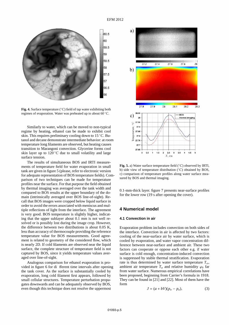
Fig. 4.Surface temperature (◦C) field of tap water exhibiting bothregimes of evaporation. Water was preheated up to about 60◦C.

Similarly to water, which can be moved to non-typicalregime by heating, ethanol can be made to exhibit coolskin. This requires preliminary cooling down to 15◦C. Bu-tanol and decane demonstrate intermediate behavior: at roomtemperature long filaments are observed, but heating causestransition to Marangoni convection. Glycerine forms coolskin layer up to 120◦C due to small volatility and largesurface tension.

The results of simultaneous BOS and IRTI measure-ments of temperature field for water evaporation in smalltank are given in figure 5 (please, refer to electronic versionfor adequate representation of BOS temperature fields). Com-parison of two techniques can be made for temperatureprofiles near the surface. For that purpose the field obtainedby thermal imaging was averaged over the tank width andcompared to BOS results at the upper boundary of the do-main (intrinsically averaged over BOS line-of-sight). Re-call that BOS images were cropped below liquid surface inorder to avoid the errors associated with meniscus and mul-tiple reflections of light from the interface. The agreementis very good. BOS temperature is slightly higher, indicat-ing that the upper sublayer about 0.1 mm is not well re-solved or is possibly lost during the image crop. However,the difference between two distributions is about 0.05 K,less than accuracy of thermocouple providing the referencetemperature value for BOS measurements. Good agree-ment is related to geometry of the considered flow, whichis nearly 2D. If cold filaments are observed near the liquidsurface, the complete structure of temperature field is notcaptured by BOS, since it yields temperature values aver-aged over line-of-sight.

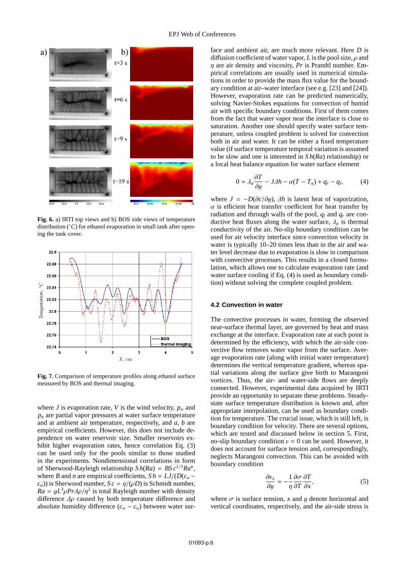
Analogous comparison for ethanol evaporation is pro-vided in figure 6 for di fferent time intervals after openingthe tank cover. As the surface is substantially cooled byevaporation, long cold filament first appears, followed bysmall cellular structures. Temperature perturbation propa-gates downwards and can be adequately observed by BOS,even though this technique does not resolve the uppermost

Fig. 5. a) Water surface temperature field (◦C) observed by IRTI,b) side view of temperature distribution (◦C) obtained by BOS,c) comparison of temperature profiles along water surface mea-sured by BOS and thermal imaging.

0.1-mm-thick layer. figure 7 presents near-surface profilesfor the lower row (19 s after opening the cover).

4 Numerical model

4.1 Convection in air

Evaporation problem includes convection on both sides ofthe interface. Convection in air is affected by two factors:cooling of the near-surface air by water surface, which iscooled by evaporation, and water vapor concentration dif-ference between near-surface and ambient air. These twofactors can cooperate or oppose each other e.g. if watersurface is cold enough, concentration-induced convectionis suppressed by stable thermal stratification. Evaporationrate is thus determined by water surface temperatureTw,ambient air temperatureTa and relative humidityϕ0 farfrom water surface. Numerous empirical correlations havebeen proposed, beginning from Carrier’s formula in 1918.They can be found in [21] and [22]. Most of them have theform

J = (a + bV)(pw − pa), (3)

01093-p.5

EPJ Web of Conferences

Fig. 6. a) IRTI top views and b) BOS side views of temperaturedistribution (◦C) for ethanol evaporation in small tank after open-ing the tank cover.

Fig. 7. Comparison of temperature profiles along ethanol surfacemeasured by BOS and thermal imaging.

whereJ is evaporation rate,V is the wind velocity,pw andpa are partial vapor pressures at water surface temperatureand at ambient air temperature, respectively, anda, b areempirical coefficients. However, this does not include de-pendence on water reservoir size. Smaller reservoirs ex-hibit higher evaporation rates, hence correlation Eq. (3)can be used only for the pools similar to those studiedin the experiments. Nondimensional correlations in formof Sherwood-Rayleigh relationshipS h(Ra) = BS c1/3Ran,whereB andn are empirical coefficients,S h= LJ/(D(cw−ca)) is Sherwood number,S c= η/(ρD) is Schmidt number,Ra = gL3ρPr∆ρ/η2 is total Rayleigh number with densitydifference∆ρ caused by both temperature difference andabsolute humidity difference (cw − ca) between water sur-

face and ambient air, are much more relevant. HereD isdiffusion coefficient of water vapor,L is the pool size,ρ andη are air density and viscosity,Pr is Prandtl number. Em-pirical correlations are usually used in numerical simula-tions in order to provide the mass flux value for the bound-ary condition at air–water interface (see e.g. [23] and [24]).However, evaporation rate can be predicted numerically,solving Navier-Stokes equations for convection of humidair with specific boundary conditions. First of them comesfrom the fact that water vapor near the interface is close tosaturation. Another one should specify water surface tem-perature, unless coupled problem is solved for convectionboth in air and water. It can be either a fixed temperaturevalue (if surface temperature temporal variation is assumedto be slow and one is interested inS h(Ra) relationship) ora local heat balance equation for water surface element

0 = λa∂T∂y− J∆h− α(T − Ta) + qr − ql , (4)

whereJ = −D(∂c/∂y), ∆h is latent heat of vaporization,α is efficient heat transfer coefficient for heat transfer byradiation and through walls of the pool,ql andqr are con-ductive heat fluxes along the water surface,λa is thermalconductivity of the air. No-slip boundary condition can beused for air velocity interface since convection velocity inwater is typically 10–20 times less than in the air and wa-ter level decrease due to evaporation is slow in comparisonwith convective processes. This results in a closed formu-lation, which allows one to calculate evaporation rate (andwater surface cooling if Eq. (4) is used as boundary condi-tion) without solving the complete coupled problem.

4.2 Convection in water

The convective processes in water, forming the observednear-surface thermal layer, are governed by heat and massexchange at the interface. Evaporation rate at each point isdetermined by the efficiency, with which the air-side con-vective flow removes water vapor from the surface. Aver-age evaporation rate (along with initial water temperature)determines the vertical temperature gradient, whereas spa-tial variations along the surface give birth to Marangonivortices. Thus, the air- and water-side flows are deeplyconnected. However, experimental data acquired by IRTIprovide an opportunity to separate these problems. Steady-state surface temperature distribution is known and, afterappropriate interpolation, can be used as boundary condi-tion for temperature. The crucial issue, which is still left, isboundary condition for velocity. There are several options,which are tested and discussed below in section 5. First,no-slip boundary conditionv = 0 can be used. However, itdoes not account for surface tension and, correspondingly,neglects Marangoni convection. This can be avoided withboundary condition

∂vx

∂y= −1

η

∂σ

∂T∂T∂x, (5)

whereσ is surface tension,x andy denote horizontal andvertical coordinates, respectively, and the air-side stress is

01093-p.6

EFM 2012

neglected. This condition provides large vertical gradientof horizontal velocity, which is observed in experiments.In fact, this boundary condition can be used to estimatevertical gradient of horizontal velocity from experimentaldata. The right-hand side of Eq. (5) is known from IRTI.Typically, for water it is about 10 s−1. Expanding the veloc-ity gradient as∂vx/∂y ∼ ∆v/δ1 and making use of typicalvelocity values, observed in PIV or numerical simulations(∆v ∼ vmax ∼ 10−3 m s−1), one arrives to an estimate forvelocity boundary thicknessδ1 about 100µm. Bulk con-vective vortices are characterized by the same velocity dif-ference, but their size is comparable with the tank size, i.e.the vorticity is at least two orders of magnitude less.

Note, however, that liquid at the surface is free to movealong the surface. It is even forced to do so by Marangonistress in the right-hand side of Eq. (5). Hence, the regimeof motionless cool skin, observed for small vertical tem-perature gradients can not be obtained using Eq. (5) asboundary condition. It is possible to combine two condi-tions mentioned above into one condition of third kind

∂vx

∂y+

hv(vx − v0)η

= −1η

∂σ

∂T∂T∂x, (6)

wherehv is effective momentum transfer coefficient (anal-ogous to heat transfer coefficient) andv0 is velocity valueprescribed at the interface. If there is no wind,v0 is set tobe zero. Relative importance of two terms in the left-handside of Eq. (6) is adjusted by the value ofBiv = hvL/η– analogue of thermal Biot number. As shown below, forhigh Biv values water velocity at the surface is decreased,leading to flow fields resembling those of cool skin regime.An important drawback is that Eq. (6) has no solid phys-ical reasoning andBiv value is a priori unknown. Anothervariant is the condition, taking into account the so calledsurface viscosityηsur f

∂vx

∂y= −1

η

∂σ

∂T∂T∂x

+ηsur f

η

∂2vx

∂x2. (7)

It should be noted that in late 80-s similar problem wasconsidered by Nunez and Sparrow [25] for geometry ofvertical open-topped tube. They dealt with a series of nu-merical models neglecting or taking into account processesof secondary (in comparison with air-side convection) im-portance: heat exchange between air inside the tube andthe ambient, heat conduction through the tube walls, con-vection in water and radiation heat transfer. However, theydid not have experimental IRTI data. Therefore, they didnot have means of solving separately water-side problemand overlooked the entire complex of problems associatedwith surface tension. Also, high Rayleigh numbers couldnot be addressed at that time because of low computationalpower.

4.3 Computational algorithm and details

Navier-Stokes equations in low Mach approximation aresolved. Compressibility effects are taken into account insimplified form, neglectingdp/dt in energy equation. This

allows using numerical methods developed for incompress-ible fluid without considering the sound waves, thus loos-ening the time step restriction. Additional equation for wa-ter vapor transport is solved for air-side problem. Volumecondensation is not taken into account, though it can takeplace locally if water is hot and temperature difference islarge. Constant thermal expansion coefficient is assumedfor water equation of state in water-side problem or, forlarge temperature variations, the complete empirical equa-tion of state [16] is incorporated into the model, increas-ing the computation time. Only 2D simulations are per-formed. Spalart-Allmaras turbulence model was used, butit appeared that it has minor influence on e.g. evaporationrate because turbulent viscosity near the water surface isclose to zero. The geometry of air-side problem presents alake-like water reservoir surrounded by horizontal flat solidwall, which is assumed adiabatic. Boundary conditions atthe water surface are given above, soft boundary condi-tions are used at upper and lateral boundaries. Ambient airtemperature and humidity, which affect evaporation rate,are specified as initial conditions. For water-side problema rectangular domain with isothermal walls is considered.The upper boundary represents free surface with specifiedsinusoidal temperature profileT(x) (mimicking IRTI datafor cellular surface structures) and boundary conditions forvelocity discussed above.

Equations are solved using second-order semi-implicitscheme. Convective terms are approximated with four-pointsupwind differences. Crank-Nicolson scheme is used for dif-fusive terms. Time integration is performed by third-orderRunge-Kutta method. Pressure is obtained by solving Pois-son equation of fractional-step method. For most simula-tions computational grids 200× 160 and 100× 50 are usedfor air-side and water-side problems, respectively. Grid stepis decreasing towards the interface. Code performance wasvalidated by solving the similar problem of natural convec-tion over the heated horizontal plate. The obtained Nusselt-Rayleigh relationship was compared to known empiricalcorrelations [26]

Nu =

{0.54Ra1/4 for laminar flow0.14Ra1/3 for turbulent flow

(8)

Deviation is small up toRa ∼ 107, when 3D effectsbecome important. At higher Rayleigh numbers heat ex-change is underestimated.

5 Simulation results

5.1 Convection in air

Flow regime is determined by the value of total Rayleighnumber, taking into account both the effects of thermaland concentration-induced convection. At negative Ray-leigh numbers (cold water case) concentration-induced con-vection is suppressed by thermal stable stratification. Hy-drodynamic velocities are small and humid air is containedwithin a thin layer near the pool surface. At large positive

01093-p.7

EPJ Web of Conferences

Rayleigh numbers turbulent convection is observed. Evap-oration proceeds in chaotic bursts, with plumes of hot hu-mid air emerging sporadically in different locations at wa-ter surface. Snapshots and time-averaged fields of relativehumidity obtained in simulations for these two regimes aredemonstrated in figure 5.1 (please, refer to electronic ver-sion). Pool size is 0.614 m,ϕ0 = 0,Ta = 27◦C, Tw = 22◦Cfor case a) and 27◦C for case b).Ra = −5.7 · 107 in casea) and 108 in case b). White rectangle represents pool sur-face. Two extreme regimes are separated by the region oflaminar convection.

Fig. 8. Snapshots (left column) and time-averaged fields (rightcolumn) of relative humidity for negative a) and large positive b)Rayleigh numbers.

Since steady state can be observed for negative andsmall positiveRa only, calculations were performed untilquasi-stationary regime was obtained. Then flow variablesand evaporation rate were recorded and averaged over along time period (e.g., 2000 s for a pool size 1 m). figure 9presents the comparison between simulation results andknown correlations for positive Rayleigh numbers. Thisimplies positive, zero or slightly negative temperature dif-ference between water and air as thermal convection usu-ally dominates over concentration-induced convection. Uni-versal curve is obtained with good accuracy for Sherwood-Rayleigh relationship irrespective of the pool size. Withinthe rangeRa = 104 − 107 good agreement is observedbetween simulation results and existing correlations. Athigher Rayleigh numbers Sherwood number is underes-timated by numerical model and certain discrepancy be-tween different correlations is also found.

Cold water situation when concentration-induced con-vection is suppressed by thermally stable stratification isless popular. Correlation by Sparrow et al. [27] is the onlyone known for this case. Nevertheless, this situation is com-mon e.g. in oceanography in upwelling phenomenon. Nu-merical results are shown in figure 10 as Sherwood numberrelation to absolute value of Rayleigh number. There is stilluniversal curve in this case, but it lies considerably lowerthan known correlation. The reason of this discrepancy isunclear and further investigation is needed.

Fig. 9. Sherwood-Rayleigh relation for positive Rayleigh num-bers: simulation results and known correlations.

Fig. 10.Sherwood-Rayleigh relation for negative Rayleigh num-bers.

5.2 Convection in water

Simulations are performed for a small square tank 2×2 cm.Temperature of the walls is 20◦C. Water surface temper-ature (except for near-wall boundary layers) varies sinu-soidally from 17.5 ◦C to 18.5 ◦C with wavelength 0.36 cm,mimicking large cells of warm water and cold water fila-ments observed experimentally in cool skin regime. Steady-state temperature and horizontal velocity fields are shownin figure 11 forBiv = 10 and 2· 104. Distances are nor-malized with respect to tank size. Note that horizontal ve-locity is shown only for the uppermost region up to depth2 mm in order to reveal the structure of the surface layer.For small values ofBiv number the liquid volume is ef-ficiently cooled with only exception for thermal bound-ary layers at the walls. Marangoni vortices are more in-tense than the Rayleigh vortices. Maximal velocities about3 cm s−1 are observed at water surface. Flow field near thesurface, dominated by Marangoni vortices, consists of pe-riodical currents along the surface with downward sinks atlocations of temperature minima. The vertical temperaturegradient is decreased by warm water reaching the surface.Generally, this scenario corresponds to experimental ob-servations made in Marangoni convection regime (for pre-heated water or ethanol and other highly volatile liquids).For largeBiv maximal horizontal velocity at the surface de-creases down to 0.1 mm s−1. Marangoni vortices are weakand the flow field of the surface layer is determined by the

01093-p.8

EFM 2012

tops of two Rayleigh vortices. The cooled layer is muchmore thin, except for the central sink of cold water pro-vided by Rayleigh convection. Water at the surface is prac-tically motionless, which corresponds to cool skin regime.

Fig. 11.Temperature in entire domain (left column,◦C) and hor-izontal velocity in surface layer (right column, m s−1) for Biv =

a) 10, b) 2· 104.

No-slip condition and Eq. (5) present extreme casesof boundary condition Eq. (6) for large and small valuesof Biv, respectively. No-slip condition does not accountfor Marangoni vortices, whereas Eq. (5) leads to surfaceliquid velocities of several cm s−1, which is incompatiblewith regime of motionless cool skin. Boundary conditionof third kind Eq. (6) yields temperature and velocity fieldssimilar to those observed in experiments, though the valueof Biv number remains an adjustable parameter, which isnot derived from properties of liquid and initial (or ambi-ent) conditions. Boundary condition with surface viscosityEq. (7) is more relevant from physical point of view. Dueto presence of velocity second derivative along the surface,it is numerically unstable, which can be fixed by choosingappropriate discretization for this term and performing sev-eral iterations to preserve accuracy. The results, similar toshown in figure 11, are obtained forηsur f ≥ 2 ·10−4 kg s−1.Note that this value is considerably higher than typicallymeasured in liquid films (10−5−10−7 kg s−1 [28]). The rea-son of such discrepancy is unclear.

6 Conclusions

Temperature fields under the surface of evaporating liquidswere studied by two independent experimental techniquesand also by means of numerical simulations. It was shownthat, depending on the liquid surface tension and volatilityas well as on initial vertical temperature gradient, two dif-ferent structures of surface layer can be obtained: motion-less cool skin and Marangoni convection. The former ischaracterized by large cells of warm liquid surrounded byfilaments of cold liquid and by surface velocity practicallyequal to zero. The latter implies small cells and movingliquid surface. Cool skin is typical for liquids with largesurface tension and/or small volatility, whereas Marangoniconvection usually takes place if surface tension is small or

evaporation is intense. Nevertheless, liquids, which typi-cally exhibit cool skin behavior, can be moved into Maran-goni mode by simple preheating, providing large verticaltemperature gradient and intense evaporation. On the con-trary, liquids, which usually form Marangoni small-scalecellular structure, can be cooled down to exhibit cool skin.In particular, water, which, as had been reported, does notexhibit Marangoni convection, can be made to do so. Com-parison of the results obtained by BOS and IRTI revealedthe lack of spatial resolution of BOS results near the liquidsurface. Nevertheless, this technique can be successfullyapplied to liquid temperature measurements in evaporationproblems since the results accuracy is better than 0.1 K. Infact, it is limited by the accuracy of thermocouple, measur-ing the reference temperature, rather than BOS accuracy.Also, this technique is extremely simple and cheap in re-alization and, along with IRTI, can be recommended foroutdoor measurements.

The performed numerical simulations demonstrate thatair- and water-side problems can be separated with helpof IRTI surface temperature data. It is shown that evap-oration rate can be calculated numerically without makinguse of empirical calculations. This requires solving air-sideproblem with appropriate boundary conditions at water–air interface: water vapor saturation and fixed water tem-perature or water temperature evolution according to localheat balance equation. Evaporation regime is determinedby the value of total Rayleigh number, taking into accountboth the effects of thermal and concentration-induced con-vection. At high Rayleigh numbers evaporation proceedschaotically, with plumes of cold humid air formed sporadi-cally at different locations. Universal curves were obtainedfor Sherwood-Rayleigh relationship in both cases of coldand hot water and compared to known empirical corre-lations. Simulations of water-side problem and compari-son with experimental data revealed the issue of boundarycondition for velocity at the surface of evaporating liquid.Boundary condition of third kind was proposed, which en-ables one to model both variants of the surface layer struc-ture. However, it contains one adjustable parameter, whichis not derived from liquid properties and/or initial condi-tions. Similar situation is observed for boundary conditioninvolving surface viscosity coefficient: simulation providesresults being in agreement with experiment only for sur-face viscosity values considerably higher than found in lit-erature. Future investigations are to solve this problem andto provide physical reasoning for these (or similar) bound-ary conditions. This might require comprehensive study ofnear-surface rheology since the surface layer is often ob-served to exhibit much more viscous behavior than the bulkliquid.

This work was partially supported by Russian Foundation for Ba-sic Research (grant 12-08-01077-a). Authors also acknowledgepartial support from M.V. Lomonosov Moscow State UniversityProgram of Development.

01093-p.9

EPJ Web of Conferences

References

1. K.B. Katsaros, W.T. Liu, J.A. Businger, and J.E. Till-man, J. Fluid Mech.,83, (1977) 311–335

2. P.J. Minnett, M. Smith, and B. Ward, Deep-Sea Re-search Part II: Topical Studies in Oceanography,58,(2011) 861–868

3. M.M. Shah, Energy and Buildings,35, (2003) 707–713

4. W.T. Liu, K.B. Katsaros, and J.A. Businger, J. Atmos.Sci.,36, (1979) 1722–1735

5. W.G. Spangenberg, W.R. Rowland, Phys. Fluids,4,(1961) 743–750

6. R.J. Volino, G.B. Smith, Exp. Fluids,27, (1999) 70–787. S.J.K. Bukhari, M.H.K. Siddiqui, Phys. Fluids,18,

(2006) 0351068. S.J.K. Bukhari, M.H.K. Siddiqui, Phys. Fluids,20,

(2008) 1221039. S.J.K. Bukhari, M.H.K. Siddiqui, Int. J. Therm. Sci.,

50, (2011) 930–93410. E.D. McAlister, W. McLeish, Appl. Opt.,9, (1970)

2697–270511. G. Meier, Exp. Fluids,33, (2002) 181–18712. K. Sefiane, C.A. Ward, Adv. Colloid Interface Sci.,

134-135, (2007) 201–22313. Yu.Yu. Plaksina, A.V. Uvarov, N.A. Vinnichenko, and

V.B. Lapshin, Russ. J. Earth Sci.,12, (2012) ES4002,http://elpub.wdcb.ru/journals/rjes/v12/2012ES000517/2012ES000517.html.

14. B. Atcheson, W. Heidrich, and I. Ihrke Exp. Fluids,46,(2009) 467–476

15. F. Scarano, M.L. Riethmuller, Exp. Fluids,26, (1999)513–523

16. W. Wagner, A. Pruss, J. Phys. Chem. Ref. Data,31,(2002) 387–536

17. P. Schiebener, J. Straub, J.M.H. Levelt Sengers, andJ.S. Gallagher, J. Phys. Chem. Ref. Data,19, (1990)677–718

18. H.E. Dillon, S.G. Penoncello, Int. J. Thermophys.,25,(2004) 321–335

19. N.A. Vinnichenko, A.V. Uvarov, and Yu.Yu. Plaksina,Proc. of the 15th Int. Symp. Flow Visualization(Minsk, Belarus), (2009) 81

20. K.A. Flack, J.R. Saylor, and G.B. Smith, Phys. Fluids,13, (2001) 3338–3345

21. M. Al-Shammiri, Desalination,150, (2002) 189–20322. S.M. Bower, J.R. Saylor, Int. J. Heat Mass Transfer,

52, (2009) 3055–306323. S.J.K Bukhari, M.H.K. Siddiqui, Heat Mass Transfer,

43, (2007) 415–42524. Z. Li, P. Heiselberg, Aalborg University, Denmark,

Report for the project ”Optimization of ventilationsystem in swimming bath”, (2005)

25. G.A. Nunez, E.M. Sparrow, Int. J. Heat Mass Transfer,31, (1988) 461–477

26. H.Y. Wong, Author,Handbook of essential formulaeand data on heat transfer for engineers(Longman,London, New York 1977)

27. E.M. Sparrow, G.K. Kratz, and M.J. Schuerger, J. HeatTransfer,105, (1983) 469–475

28. A.W. Adamson, Physical chemistry of surfaces(Wiley-Interscience, New York 1997)

01093-p.10