Ch

Ma

b

a

ARRAA

KHSMDR

1

vehhfdtrse

ascittc

0d

Journal of Chromatography A, 1216 (2009) 1439–1449

Contents lists available at ScienceDirect

Journal of Chromatography A

journa l homepage: www.e lsev ier .com/ locate /chroma

ombined column–mobile phase mixture statistical design optimization ofigh-performance liquid chromatographic analysis of multicomponent systems

árcia C. Breitkreitza, Isabel C.S.F. Jardimb, Roy E. Brunsb,∗

IIPF, International Institute of Pharmaceutical Research, 13186-481, Hortolândia, SP, BrazilInstitute of Chemistry, State University of Campinas, P.O. Box 6154, 13083-970, Campinas, SP, Brazil

r t i c l e i n f o

rticle history:eceived 22 September 2008eceived in revised form 11 December 2008ccepted 31 December 2008vailable online 8 January 2009

eywords:

a b s t r a c t

A statistical approach for the simultaneous optimization of the mobile and stationary phases usedin reversed-phase liquid chromatography is presented. Mixture designs using aqueous mixtures ofacetonitrile (ACN), methanol (MeOH) and tetrahydrofuran (THF) organic modifiers were performed simul-taneously with column type optimization, according to a split-plot design, to achieve the best separationof compounds in two sample sets: one containing 10 neutral compounds with similar retention factorsand another containing 11 pesticides. Combined models were obtained by multiplying a linear model

PLCplit-plot designsobile phase optimizationerringer’s desirability functionesponse surface analysis

for column type, C8 or C18, by quadratic or special cubic mixture models. Instead of using an objectiveresponse function, combined models were built for elementary chromatographic criteria (retention fac-tors, resolution and relative retention) of each solute or pair of solutes and, after their validation, theglobal separation was accomplished by means of Derringer’s desirability functions. For neutral com-pounds a 37:12:8:43 (v/v/v/v) percentage mixture of ACN:MeOH:THF:H2O with the C18 column and for

/v) A

pesticides a 15:15:70 (v/vall peaks.

. Introduction

In all scientific research, it is interesting to find out whichariables can affect the system and how they do so. Statisticalxperimental design is a multivariate optimization technique thatas been widely used for some time in many research fields andas been recognized as a useful tool for chemists and engineers

or several reasons: (1) interactions between variables can only beetected using multivariate methods, (2) the multivariate parame-ers of models are more accurate than single measurements (3) theesearcher can systemize his work in a much more objective way,aving time and resources and (4) all variables are treated withqual importance, minimizing the risk of wrong assessments.

In our study, there are two main groups of variables, process vari-bles and mixture variables. While variables of the first group aretatistically independent and can be freely varied within the physi-al and chemical constraints of the system, mixture variables are notndependent, since their sum must always be constant and equal

o 100%. In this kind of design, the chemical and physical proper-ies are studied as a function of varying proportions of the mixtureomponents.

∗ Corresponding author. Tel.: +55 19 35213106; fax: +55 19 35213023.E-mail address: bruns@iqm.unicamp.br (R.E. Bruns).

021-9673/$ – see front matter © 2009 Elsevier B.V. All rights reserved.oi:10.1016/j.chroma.2008.12.093

CN:THF:H2O mixture with the C8 column provide excellent resolution of

© 2009 Elsevier B.V. All rights reserved.

The mobile and stationary phase compositions in HPLC are morelikely to affect a particular separation than any other factor, such astemperature or mobile phase flow rate. Mobile phase optimizationprocedures are normally based on the solvent selectivity triangle,first described by Snyder [1] and Rohrschneider [2] in which organicmodifiers are classified according to their ability to interact withthe solute as a proton donor (basic), a proton acceptor (acidic) ora dipole. Solvents that are located far away from each other in thistriangle have the largest differences in these properties and, hence,greater differences in selectivity will be found when using them inthe mobile phase. Considering miscibility, ease of use, availabilityand reasonable boiling point as well [3], the best organic solventchoices for reversed-phase HPLC are acetonitrile (ACN), methanol(MeOH) and tetrahydrofuran (THF).

The most frequently used columns in reversed-phase liquidchromatography are the C8 and C18 bonded phases. It is knownthat solutes behave differently in each column owing to differentinteractions between them and the organic chain bonded to silica,giving rise to differences in separation. Furthermore the optimizedmobile phase mixture for one column will not necessarily be opti-mum for the other. Thus, the choice of the column that will give

desired results is not often straightforward and, because of that,these stationary phases were selected for this study.

After organic modifier selection, two different approaches canbe carried out: (1) water can be considered as one of the mobilephase components or (2) only as the carrier or diluent of organic

1 matog

matmvmacl[uctcr

eoqaattActfintpcivtc

mdeiirwadcacgtieetHdsaatc

psTu

440 M.C. Breitkreitz et al. / J. Chro

odifiers. In the first approach, the system can be described bytetrahedron in which the pure components are represented at

he vertices. This strategy is very useful in gradient analysis opti-ization [4–6] since solvent strength, besides solvent selectivity, is

aried. On the other hand, considering water as a diluent, aqueousixtures of the organic modifiers are actually the mixture vari-

bles. The water content is chosen so that all the mobile phaseompositions present similar elution strengths and thus, a simi-ar k-range for all the solutes. In this manner, Snyder and Kirkland7] described a simplex-based method for optimization strategiessing aqueous mixtures of ACN, MeOH and THF for reversed-phasehromatography. However, it is interesting to note that, althoughhis procedure sometimes does allow a good separation of theompounds of interest, normally no statistical treatment for theesulting data is provided.

Besides the lack of statistical treatment available in the lit-rature, the greatest drawback concerning this chromatographicptimization procedure is to find a good way of describing theuality of the separation for different experimental conditions. Thepproach normally used reports the overall separation by means ofn objective function or an optimization criterion calculated fromhe usual chromatographic parameters (retention times, resolu-ion, peak areas etc.), which should reflect the researcher’s goals.lthough one might think that representing the quality of the wholehromatogram is only an extension of representing the quality ofhe separation of a pair of peaks, it is not a straightforward task tond an adequate function and this difficulty has resulted in a largeumber of objective functions proposed and reviewed in the litera-ure [8–14] to address this problem. Siouffi and Phan-Tan-Luu [15]oint out the existence of more than a dozen objective functionsoncluding there is no definitive response function for optimizationn chromatography and capillary electrophoresis. This subject isery detailed and extended and a more complete analysis is beyondhe scope of this paper. A fairly complete review of optimizationriteria has been addressed by Schoenmakers [16].

Derringer’s desirability functions [17] have been used in chro-atography and electrophoresis as an approach from multicriteria

ecision making (MCDM) for simultaneous optimization of sev-ral chromatographic goals. Bourguignon and Massart [18] usedt to choose the best chromatogram considering separation qual-ty (measured by the calibrated normalized resolution product,*), the analysis time and peak asymmetry. The variables studiedere the fraction of methanol and the pH of a buffer. Jimidar et

l. [19] proposed the use of Derringer’s desirability function toetermine the conditions that will result in the most desirableombination of separation, sensitivity and analysis time with theid of a central composite design for two variables, pH and theoncentration of a complexing agent in the buffer electrolyte. Man-elings et al. [20] have used a central composite design to studyhe influence of the chiral selector concentration and organic mod-fier on retention and resolution in chiral separation by capillarylectrochromatography; a similar design was used by Sivakumart al. [21] to optimize HPLC separation of domperidone and pan-oprazole along with Derringer’s desirability functions. Safa andadjmohammadi [22] employed a composite design in a cubicalomain for simultaneously optimizing the resolution and analy-is time in micellar liquid chromatography of phenyl thihydantoinmino acids using Derringer’s desirability function. Mixture designnd desirability functions were used by Furlanetto et al. [23] forhe optimization of a microemulsion system for the eletrokinetichromatographic determination of ketorolac and its impurities.

Vander Heyden and co-workers [24] have used principal com-onent and hierarchical cluster analysis in the development ofelective methods to characterize impurities in drug substances.he Derringer and Pareto – optimality approaches [26] were veryseful for column selection in a study by this same laboratory

r. A 1216 (2009) 1439–1449

[25]. Cela and co-workers used an evolutionary algorithm speciallydeveloped to map gradient elutions of ternary solvent mixtures.Torres-Lapasió and co-workers [27] proposed an optimizationmethodology in HPLC for the selection of two or more mobilephases having optimal complementary resolution. Also a reviewon total, partial and specific resolutions of compounds in mixtureshas been recently published [28].

The objective of this paper is to describe an optimizationprocedure for reversed-phase liquid chromatography based onDerringer’s desirability function and combined models concern-ing simultaneously a three-component mixture design for mobilephase optimization and a process factor, the column type. Firsta statistical design is made involving mixtures of three aqueousorganic modifier solutions and both the C8 and C18 columns. Sec-ond, polynomial process–mixture variable models are fitted to theindividual chromatographic criteria (retention factor, resolution orrelative retention) for each analyte or pair of analytes. Individualresponses for each solute or pair of solutes will be shown hereto follow simpler models than global objective functions that tryto characterize all peaks simultaneously with consequent loss ofimportant information for the optimizing process. Thus, successfulmodel validation is more likely. In a last step the Derringer–Suichdesirability function is applied to the combined process–mixturevariable models to simultaneously optimize the position of everypeak so that good quality chromatographic separation is achieved.The split-plot design [29–32] was used since the simultaneousoptimization of process and mixture factors results in operationaldifficulties due to the large number of experiments involved. Theseshould be executed randomly in order to obtain accurate error esti-mates for testing model significance and validity. The completerandomization recommendation is relaxed using this kind of designso that frequent chromatographic column changes are avoided dur-ing experimentation. It should be emphasized that both combinedprocess–mixture variable optimization and split-plot proceduresare rarely encountered in the chemical literature.

To show the potential usefulness of our procedure two samplemixtures with very different types of compounds were investigated.The general strategy was first developed by analyzing a mixtureof 10 neutral compounds. The potential usefulness of the devel-oped method was then tested by optimizing the mobile phase forthe investigation of 11 pesticides. Samples of this kind involvingcompounds from different classes are treated very often in ourlaboratory for method development and validation of pesticidemultiresidues in different matrices.

2. Experimental

2.1. Chemicals and materials

ACN, MeOH and THF were all HPLC grade from Tedia and wereused to prepare the mobile phases. Water purified by a Milli-Q system from Millipore (Bedford, MA, USA) was used to adjustthe chromatographic strengths. All mobile phases were filteredemploying a 0.22 �m poly(vinylidene difluoride) (PVDF) MilliporeGV (Durapore) membrane and were stored in 1 L amber flasks.Before each run, the mobile phases were degasified by passing a100 kPa helium flow for 5 min. During the runs the helium pressurewas 30 kPa.

2.2. Preparation of the solution of neutral compounds and

pesticides

The neutral compounds used for preparation of the test solutionare listed in Table 1. They were selected because their separationsare difficult to achieve by isocratic elution using aqueous mixtures

M.C. Breitkreitz et al. / J. Chromatog

Table 1Analytes present in the mixture of neutral compounds with their respective sourcesand concentrations.

Compound Sources Concentration (mg/mL)

Uracil Aldrich 1.0 × 10−2

Phenol Labsynth 1.8 × 10−1

�-Naphthol Vetec 6.0 × 10−2

�-Naphthol Vetec 1.5 × 10−1

Naphthalene Vetec 8.4 × 10−1

�-Methyl naphthyl ether * 2.0 × 10−1

Toluene Tedia 1.4 × 10−3

BBN

oTtT

99abmSg

crsts1te1cwrwwo

2

uUaucucrtfl2

idwdpmt

an important model in our application. The factor–mixture variable

enzene Labsynth 1.0 × 10−3

enzonitrile Aldrich 0.1 × 10−3

,N-Dimethylaniline Aldrich 0.02 × 10−3

f normally employed organic modifiers, such as ACN and MeOH.he samples were prepared and dissolved in the compositions ofhe mobile phase corresponding to each point of the mixture design.able 1 also lists the concentrations of each analyte.

The pesticide standards were: imazetapyr (Chem Service,9.0%), imazaquin (Chem Service, 99.0%), ametryn (Novartis6.8%), cyanazine (Novartis, 98.0%), simazine (Novartis, 98.3%),trazine (Chem Service, 98.0%), bentazone (Guará, 99.9%), car-aryl (Supelco 98.0%), carboxin (Chem Service, 99.0%), thiophanateethyl (Riedel-de Haen, 99.8%) and metsulfuron methyl (Chem

evice 98.0%). The chemical structures of these compounds areiven in Supplementary Fig. S1.

With the exceptions of simazine and carbaryl, the following pro-edure was followed to prepare the stock solutions of each of theeference pesticides: 0.010 g of the pure solid compound was dis-olved in 10 mL of a 70:30 (v/v) acetonitrile–water mixture so thathe resulting solutions had a 1000 �g/mL concentration. 150 �L oftock solution of each reference compound were transferred to a0 mL volumetric flask containing a solvent mixture correspondingo a mixture design point. In this way the concentration of each ref-rence compound in the mixture was about 15 �g/mL. For carbaryl00 �L were transferred to the mixing flask and its final con-entration was approximately 10 �g/mL. 0.060 g of simazine wereeighed and dissolved in 20 mL of pure acetonitrile, so that the

esulting concentration was 3000 �g/mL. 500 �L of this solutionere transferred to the mixing flask so that the final concentrationas about 150 �g/mL. The concentration of simazine was higher

wing to its low sensitivity.

.3. Chromatographic instrumentation and conditions

All separations were carried out on a modular Shimadzu liq-id chromatograph equipped with: Model SPD 10 AD diode arrayV–vis absorbance detector (190–900 nm wavelength range) withn 8 �L cell; auto-sampling injector model SIL 10 AD, sample vol-me set at 10 �L; column oven model CTO 10 AS and systemontroller SCL 10A, equipped with Class-VP software. The columnssed were bonded phase SGE Wakosil II C18 or C8 columns (parti-le size 5 �m, 150 mm × 4.6 mm I.D.), without guard columns. Theuns for analyses of neutral compounds and for the mixture of pes-icides were performed at 25 ◦C, with a 1.0 mL/min mobile phaseow rate. The neutral and pesticide compounds were detected at54 and 210 nm, respectively.

The statistical design’s “pure” components were organic mod-fier – water mixtures at equal chromatographic strengths. Toetermine the organic modifier:water proportions an initial runith ACN:H O 80:20 (v/v) was made with subsequent runs with

2iminishing proportions of ACN in order to find an ACN–H2O pro-ortion that furnished retention factors between 0.5 and 10 for theixture of neutral compounds. Transference equations were used

o estimate MeOH:H2O and THF:H2O proportions that furnished

r. A 1216 (2009) 1439–1449 1441

approximately the same chromatographic strength. The exact pro-portions were then adjusted experimentally. The same procedurewas used for the pesticide mixtures except that an ACN:H2O 50:50(v/v) mixture was used in the initial run. In this case the pH of thewater was adjusted to 3 by the addition of phosphoric acid so thatall the compounds were in their protonated forms.

2.4. Experimental design and data treatment

A mixture simplex-centroid design with axial points [33,34] andreplicates at each point was applied to both C8 and C18 columnsin a mixture design containing the column as a process variable.The experimental domain for the neutral compound samples wasrestricted based on prior experiments and the mixture variableswere thus represented by pseudocomponents for the calculations.The first seven points were used for model construction and lack offit tests and the remaining three were used to check the calculatedmodel. Experiments were carried out using a split-plot approach,the column was fixed at one level and all of the experiments wereperformed randomly by changing the mobile phase compositionof the 10 points. Then the column was changed and the same10 mixture experiments were randomly executed. Replicates wereperformed by repeating the procedure described above. As a firstattempt to use an elementary criterion for modeling, the retentionfactors were used as responses to model the separation of sevenneutral compounds (the selected compounds were those that pre-sented separation problems in pure mobile phase compositions).Then, resolution was used to model the separation of these sevencompounds and relative retention to model the separation of fourpesticides from the second mixture. The models were validated byanalysis of variance (ANOVA) and the predicted results obtained forthe three check blends. Finally, a desirability value was establishedfor each response and the desired separation was found by com-bining them into a global desirability function. Calculations werecarried out by Design Expert (Design Expert 6.0.10, Minneapolis,MN, USA) and Matlab (The Mathworks, Matlab 7.0.4, Natwick, MA,USA) programs.

3. Statistical modeling and validation

3.1. Process–mixture variable models

Process–mixture combined models can be obtained by multi-plying mixture models by independent-variable models (factorial

models) such as the linear y = ˛0 +m∑

i=1

˛izi and bi-linear y = ˛0 +

m∑

i=1

˛izi +m∑

i=1

m∑

j /= i

˛ijzizj models. These models describe interaction

effects showing how factor levels can influence blending proper-ties of mixtures or how different mixtures show different effectson changing factors levels for one process variable, column typein our study. Multiplying the linear model, y = ˛0 + ˛1z1, by thespecial cubic mixture model yields

y = g01x1 + g0

2x2 + g03x3 + g0

12x1x2 + g013x1x3 + g0

23x2x3 + g0123x1x2x3

+ g11x1z1+g1

2x2z1 + g13x3z1 + g1

12x1x2z1 + g113x1x3z1 + g1

23x2x3z1

+ g1123x1x2x3z1, (1)

interaction terms will be important for systems where the opti-mized mobile phase mixture for one column is different than theoptimal one for the other. More details on this topic can be foundin Ref. [30].

1442 M.C. Breitkreitz et al. / J. Chromatogr. A 1216 (2009) 1439–1449

Table 2Analysis of variance (ANOVA) for split-plot designs.

Variation source Sum of squares (SS)* Degree of freedom Mean sum of squares (MS)

Replicates (R) SSR = mp

r∑

i=1

(Ri − �)2

r − 1 MSR = SS/(r − 1)

Main-plot (Z) SSZ = mr

p∑

i=1

(Zi − �)2

p − 1 MSZ = SSZ/(p − 1)

Main-plot error (RZ) SSRZ = m

r∑

i=1

p∑

i=1

(Zij − Zi − Ri − �)2

(r − 1)(p − 1) MSRZ = SSRZ/(r − 1)(p − 1)

Sub-plot (X) SSX = pr

m∑

i=1

(Xi − �)2

m − 1 MSX = SSX(m − 1)

M

p∑ m∑

S

3

todridmr

lt

y

TNs

b

w

C

T

V

wzidct

ietfadtitus

ain-plot–sub-plot (ZX) SSZX = r

j=1 k=1

(Zjk − Zj − Xk − �)2

ub-plot error (RX + RZX) Obtained by difference**

.2. Split-plot procedures

The large number of experiments to be made in the simul-aneous optimization of mixture and process variables result inperational difficulties since an accurate error estimate implies ran-omization of all the experiments [33,34]. These difficulties can beeduced using the split-plot strategy [30]. Different mixture exper-ments are carried out for each of the p conditions of the factorialesign and these are randomized as recommended for any simpleixture design. The p different factorial blocks are also executed

andomly.Although it facilitates laboratory work, the split-plot procedure

eads to a statistical model with a more complex error structurehan the one for which complete randomization is performed,

= f (z1.....zqx1......xq′ ) + ı + ε (2)

wo error contributions are present, the main-plot error, ı ≈(0, �2

MP), and the sub-plot error, ε ≈ N(0, �2SP). Generalized least

quares regression should be used to determine this model [30].

GLS = (XtV−1X)−1

XtV−1y−→ (3)

ith the covariance matrix given by

ov(bGLS) = (XtV−1X)−1

(4)

he V matrix is given by

= �2MPJ + �2

SPI (5)

ith J being a block diagonal matrix with ones in the blocks anderos elsewhere while I is the identity matrix. This equation nicelyllustrates the cost of not running experiments in a completely ran-om order. The experimental error is expected to consist of bothorrelated (systematic error) and uncorrelated (random error) con-ributions.

The analysis of variance in this case is quite different becausenstead of one variance estimate evaluated from replicates of allxperiments two experimental error sources are obtained, one fromhe sub-plot or mixture treatments (�SP

2) and the other from theactorial or main-plot treatments (�MP

2). Furthermore, to obtainccurate measures of the main and sub-plot variances, duplicateeterminations of all experiments are recommended. Since replica-

ions are executed in blocks there is also a replication variance, �R

2

n the split-plot analysis of variance. The entire split-plot ANOVAable is shown in Table 2. Significance testing is similar to that in reg-lar ANOVA, except that there are two error terms. The main-plotum of squares is used to test the significance of the factorial process

(p − 1)(m − 1) MSZX = SSZX/(m − 1)(p − 1)

p(r − 1)(m − 1) MSe = SSe/p(r − 1)(m − 1)

variable effects whereas the significance of the mixture variableeffects and the mixture–process variable interaction effects use thesub-plot error to obtain Fcalc. More details on split-plot design canbe found in Ref. [30].

4. Results and discussion

4.1. Chromatographic strength determination of the mobilephases

The ACN, MeOH and THF organic modifiers were chosen basedon the selectivity triangle proposed by Snyder [1] for reversed-phase HPLC. Besides having good miscibility with water (the diluentsolvent in reversed-phase), easy handling, and reasonable boilingpoints, these modifiers present large differences in physical proper-ties and thus, large differences in selectivity are likely to be obtainedin the chromatograms. Aqueous mixtures of these organic modifierswere the mixture variables, i.e. the xi. The ACN:H2O, MeOH:H2Oand THF:H2O proportions were defined as follows: First, the sol-vent strength of ACN in water was varied to produce a k-range ofabout 1–10 for all the compounds. This was achieved in several runsusing the C18 column and by gradually decreasing the ACN content.For the mixture of neutral compounds, the best chromatographicstrength was reached with ACN:H2O 55:45 (v/v), for which the kvalue range was 0.9–8.0. Once this composition had been experi-mentally determined, the water content of the other solvents werepredicted using the equation: �2 = (�1S1)/S2 where �1 is the volumefraction of organic modifier 1 (known) and �2 is the volume fractionof organic modifier 2 (to be determined) and S1 and S2 are the corre-sponding solvent reversed-phase polarities [7]. Since this equationprovides only an estimate, small experimental adjustments aroundthe predicted values were performed. In this manner, the other twoorganic modifier contents were determined to be MeOH:H2O 70:30(v/v) and THF:H2O 50:50 (v/v) solutions. For the pesticide sample,the compositions of the pure mixture variables were determined inthe same way and the selected proportions were: ACN:H2O 30:70,MeOH:H2O 45:55 and THF:H2O 30:70 (v/v).

4.2. Determination of mobile phase compositions for the design

The mobile phase compositions to be used for model build-

ing and validation were selected by means of a simplex-centroiddesign, with axial check points, as shown in Fig. 1.

The center points of each side of the triangle are 50–50% mix-tures of the solutions from their corresponding vertices. The centerpoint of the triangle is an equal volume mixture of the three

M.C. Breitkreitz et al. / J. Chromatog

Fig. 1. Simplex-centroid design with axial check points indicating the mobile phasecompositions used for model building and validation: XACN = ACN:H2O 55:45 (v/v)fX(c

vtFtaapo0rtcd

ar

x

wxotamoaap

4

cpemttpcfi

or the mixture of neutral compounds and 30:70 (v/v) for the pesticide mixture;MeOH = MeOH:H2O 70:30 (v/v) for the mixture of neutral compounds and 45:55v/v) for the pesticide mixture; XTHF = THF:H2O 50:50 (v/v) for the mixture of neutralompounds and 30:70 (v/v) for the pesticide mixture.

ertex solutions. The check points, 8–10, represent mixtures con-aining 2/3 of one vertex mixture and 1/6 of each of the other two.or the neutral compound sample, the simplex-centroid points inhe region defined by 0.5 ≤ MeOH:H2O ≤ 1.0, 0.5 ≤ THF:H2O ≤ 1.0nd consequently 0 ≤ ACN:H2O ≤ 0.5, i.e. large quantities of MeOHnd THF, resulted in chromatograms with excessively overlappedeaks. For this reason the experimental domain was reduced andnly mixtures with 0.5 ≤ ACN:H2O ≤ 1.0, 0 ≤ MeOH:H2O ≤ 0.5 and≤ THF:H2O ≤ 0.5 were investigated. The experimental domain cor-

esponds to the triangle formed by points 1, 4 and 5 that becamehe vertices of the reduced simplex-centroid design for the neutralompounds. Side midpoints and triangle interior points were thenetermined by mixing the 1, 4 and 5 aqueous solutions accordingly.

Since this is a reduced triangular region inside the main tri-ngle, the mobile phase compositions could be re-calculated andepresented by pseudocomponents,

ip = xi − ai

1 −q∑

i=1

ai

(6)

here xip is the proportion of the solvent in pseudocomponents;i represents the original proportion of solvent i (in the trianglef ternary mixtures, Fig. 1) and ai is the lower limit of solvent i inhe experimental domain. Pseudocomponent transformations [30]re commonly used to provide better conditioning of the X designatrix for calculations. The component proportions of the aqueous

rganic modifiers, the pseudocomponent values and the percent-ge compositions of the simplex-centroid and axial point mixturesre given in Supplementary Tables S1 and S2 for the neutral andesticide compounds.

.3. Process variable assessment

A 1.0 mL/min flow rate was determined by van Deemter’s pro-edure and kept constant throughout the experiments. It has beenreviously observed that using higher values of flow rate causesxcessive peak overlap whereas lower values bring no improve-ents in separation while increasing analysis time and inflating

he precision of repeated measurements. The temperature was alsoested in screening experiments. An increase in temperature did notrovoke any change in the separation of the neutral compounds andaused peak overlap for the pesticide sample. For this reason, it wasxed at 25 ◦C.

r. A 1216 (2009) 1439–1449 1443

Two types of stationary phases (C8 or C18) were investigated.The chronology of column and mobile phase changes followed thesplit-plot scheme discussed earlier.

4.4. Response selection

The response used in experimental designs is a property orparameter that allows the assessment of the quality of results underdifferent experimental conditions. The criteria used to describe achromatographic separation can be classified into two differentgroups: elementary criteria – such as resolution (Rs), separationfactor (˛) and relative retention (RR), which describes the separa-tion of a single pair of compounds – and response functions, whichare combinations of elementary criteria made by using differentmathematical operations, such as the sum, product or logarithm.Besides good chromatographic separation, reasonable analysis timeis normally desired and the optimization problem becomes morecomplicated when these two criteria are in conflict. The approachoften used is to combine these objectives into a response function,which consist of a summation/product of one term related to timeand another that describes the separation quality with both havingweighting factors selected by the researcher.

Although response functions are combinations of elemen-tary criteria, they may not reflect the quality of the overallchromatogram and sometimes their use can be misleading. Further-more, the choice of the weighting factors is arbitrary and completelydepends on the researcher: the choice of different weighting factorscan lead to ambiguous results. Here a variety of response functionswere used to treat the chromatographic data reported in this paper.

In all cases modeling these response functions led to significantlack of fit. For this reason the response functions were abandonedfor the use of elementary criteria. Their dependence on mixtureand factor variable levels was seen to be much simpler than forthe response functions and can be described by accurate modelsthat have no significant lack of fit. Conditions resulting in overallseparation in a reasonable analysis time can then be found by meansof the Derringer and Suich [17] desirability function.

Derringer and Suich described a procedure for the simulta-neous optimization of several responses. First, the value of eachresponse, represented by yi, is calculated over the experimentaldomain by using the corresponding model equation. By using pos-tulated desirability functions, a partial desirability, that varies from0 to 1, depending on the proximity of the model and desired val-ues, is calculated for each response over the experimental domainand then the individual desirabilities are combined into a globaldesirability (D) by means of a geometric mean. It is important torecall that the search for the desired conditions is performed usingthe models obtained for each elementary response. In this way, itis important that the models are accurate representations of theexperimental data and are properly validated having no lack of fit.

4.5. Retention factor (k) models and validation

Combined models obtained by multiplying a quadratic or spe-cial cubic mixture model by a linear model for describing columnbehavior were used to describe the variations in the retention fac-tors. The retention values are tabulated in Supplementary TablesS3 and S4. For the mixture of neutral compounds, only thosecompounds presenting separation problems in the pure mobilephase compositions, benzonitrile, �-naphthol, �-naphthol, ben-zene, toluene, �-methyl naphthyl ether, toluene and naphthalene,

were modeled. The summary of the split-plot analysis of variancefor all the combined models is shown in Table 3.

Statistical significance of main-plot treatment (related to thecolumn type) was tested by comparing the main-plot meansquare/main-plot error ratio to the F1,1,95% value, which is 161.4. For

1444 M.C. Breitkreitz et al. / J. Chromatogr. A 1216 (2009) 1439–1449

Table 3Summary of split-plot analysis of variance for statistical significance of main-plot, sub-plot, and main-plot–sub-plot treatments as well as model lack of fit.

Model Main-plot treatment Sub-plot treatment Main-plot–sub-plot Lack of fit

Benzonitrile 576.200 1,406.500 4.00 1.989�-Naphthol 738.357 177.000 7.666 1.540�-Naphthol 786.381 137.800 4.600 0.486Benzene 1,327.300 1,108.750 10.000 2.475Toluene 1,380.116 508.060 15.933 1.512�-Methyl naphthyl ether 2,201.890 622.120 71.879 2.395Naphthalene 2,644.230 509.000 52.580 1.368F critical values F1,1,95% = 161.4 F5,12,95% = 3.11 F2,12,95% = 3.89

Table 4Observed and predicted values of retention factors of the three axial check points (8, 9 and 10, Fig. 1) with the C8 column.

Compound P8 P9 P10

Predicted Observed Predicted Observed Predicted Observed

Benzonitrile 1.18 1.13 0.85 0.83 0.95 0.92�-Naphthol 1.41 1.37 1.24 1.22 1.38 1.32�-Naphthol 1.64 1.60 1.46 1.47 1.63 1.57BT�N

aMccb

mmmtIirara

vpatitttaects

TO

C

B��BT�N

enzene 1.91 1.84oluene 2.72 2.64-Methyl naphthyl ether 3.33 3.24aphthalene 3.43 3.35

ll models, main-plot treatment was found to be very significant.oreover, the more the main-plot sum of squares increases, indi-

ating increasing differences between the retention factors of theseolumns, the more the columns retain the compounds, as expectedased on chromatographic theory.

Similarly, for sub-plot and main-plot–sub-plot interaction treat-ents the significance was tested by comparing the sub-plotean square/sub-plot error and main-plot–sub-plot interactionean square/sub-plot error ratios with the F5,12,95% value. All these

reatment sums of squares were found to be very significant.t is interesting to notice that the more the main-plot–sub-plotnteraction sum of squares increases the more the compound isetained. The graphs of retention factor vs. design points for slightlynd strongly retained compounds, benzonitrile and naphthalene,espectively, are shown in Supplementary Fig. S2. Replicate resultsre shown side by side.

From examination of the graphs in Supplementary Fig. S2 andalues in Table 3, one can verify that for a slightly retained com-ound, benzonitrile, the retention is similar in both columns, whichccounts for the lower value of main-plot sum of squares, in relationo a more retained compound. Moreover, the main-plot–sub-plotnteraction is only slightly significant, which can be seen fromhe similar profiles of the two curves along the design points. Onhe other hand, for a more retained compound, like naphthalene,he differences in retention in each column is more significant,

s was already expected for the reversed-phase columns, whichxplains its higher main-plot sum of squares. Furthermore, for thisompound, the profiles of the curves are different, indicating thathe mixture compositions behave differently in each column, con-istent with the increasing main-plot–sub-plot interaction sum

able 5bserved and predicted values of the retention factors of the three axial check points (8, 9

ompounds P8

Predicted Observed

enzonitrile 1.41 1.37-Naphthol 1.80 1.77-Naphthol 2.15 2.11enzene 2.66 2.58oluene 4.12 4.03-Methyl naphthyl ether 5.29 5.17aphthalene 5.60 5.49

1.49 1.47 1.69 1.632.22 2.21 2.39 2.292.81 2.81 2.64 2.532.86 2.81 2.83 2.71

of square values as compound retention increases. Model lack offit was calculated by comparing the calculated F value, given by[30]:F = (m−q)MSX /p(m−q)

MSe+ (p−1)(m−q)MSXZ/p(m−q)

MSeto the tabulated F

value (F2,12,95% = 3.89). No models had lack of fit since all the valuesin the last column of Table 3 are lower than 3.89.

Seven design points (1–7, see Fig. 1) were used for model build-ing and three axial points (8–10) as an external set for validation.Normal probability graphs of the residuals and the residual vs.predicted value graphs indicate that the residuals follow normaldistributions, with no indication of heteroscedastic behaviors. Thegraphs of predicted vs. observed values for the seven design pointsare given in Supplementary Fig. S3. The prediction of the threeexternal check points (Tables 4 and 5) indicate excellent fits forthe models of all analytes. For all graphs of predicted vs. observedvalues, the linear coefficient was not significant, indicating no sys-tematic errors for the models. The 95% confidence intervals for theline slopes all included 1 and the correlation coefficient was alwaysabove 0.997.

Analyzing the mathematical expressions of the models and per-forming t-tests using the coefficient/error ratios it is possible toverify which terms contribute most to the high sums of squaresobserved in Table 3. These ratios should be compared with the crit-ical t distribution values using p(r − 1)(m − 1) degrees of freedom forthe coefficients of pure mixture variables and using Satterthwaite’sapproximation to estimate the number of degrees of freedom in the

case of coefficients containing both process and mixture variables[30]. However, as a rough guide, coefficient/error ratios higher than3 can be considered significant. The significant coefficients in theproposed model are shown in Table 6. As can be observed there,the linear and quadratic pure mixture coefficients and bi-linear

and 10, Fig. 1) with the C18 column.

P9 P10

Predicted Observed Predicted Observed

1.04 1.05 1.14 1.141.66 1.72 1.74 1.731.99 2.07 2.11 2.092.17 2.24 2.36 2.353.51 3.66 3.56 3.534.74 4.96 3.98 3.994.91 5.17 4.40 4.40

M.C. Breitkreitz et al. / J. Chromatogr. A 1216 (2009) 1439–1449 1445

Table 6Significant coefficients of combined models for retention factors of the overlapped compounds in the mixture of neutral compounds.

Coefficient Benzonitrile �-Naphthol �-Naphthol Benzene Toluene �-Methyl naphthyl ether Naphthalene

A (ACN) 1.604 1.669 1.951 2.647 3.923 4.975 5.192B (MeOH) 0.886 1.369 1.623 1.710 2.753 3.830 3.829C (THF) 1.071 1.534 1.818 2.042 2.940 2.960 3.277AB −0.447 −0.167 −0.213 −0.626 −0.718 −0.396 −0.618AC −0.367 0.223 0.327 −0.311 −0.513 −0.776 −0.553AD 0.117 0.182 0.225 0.405 0.770 1.121 1.229BC −0.262 0.133 0.252 – – −0.326 –BD 0.090 0.217 0.248 0.332 0.645 1.056 1.056CD 0.095 0.157 0.208 0.325 0.568 0.551 0.664ABD – – 0.142 – – 0.162 –ACD – – – – – – –BCD – – – – – – –D = column

Table 7Errors estimates of the coefficients of the models describing benzonitrile, benzene and naphthalene retentions according to the split-plot and complete randomizationapproaches.

Coefficient Benzonitrile Benzene Naphthalene

Random Split-plot Random Split-plot Random Split-plot

A 0.007 0.006 0.013 0.010 0.032 0.029B 0.007 0.006 0.013 0.010 0.032 0.029C 0.007 0.006 0.013 0.010 0.032 0.029AB 0.032 0.029 0.058 0.048 0.145 0.137AC 0.032 0.029 0.058 0.048 0.145 0.137AD 0.007 0.007 0.013 0.014 0.032 0.033BC 0.032 0.029 0.058 0.048 0.145 0.137BD 0.007 0.007 0.013 0.014 0.032 0.033C .013A .058A .058B .058

pna

eeufihmazTs

TS

C

ABCAAABBCAAABAD

D 0.007 0.007 0BD 0.032 0.029 0CD 0.032 0.029 0CD 0.032 0.029 0

ure mixture–column type interaction coefficients tend to be sig-ificant whereas the quadratic mixture–column type interactionsre not.

Considering that the experimental variance will have differ-nt impacts on the coefficient errors depending on whether thexperiments have been performed in a completely random order orsing a restricted randomization approach, like split-plot, the coef-cient errors were re-calculated supposing that the experimentsad been carried out in a completely random order. The errors of theodel coefficients for a slightly retained compound (benzonitrile),

compound with intermediate chromatographic retention (ben-

ene) and a very strongly retained one (naphthalene) are shown inable 7 where comparisons can be made between the random andplit-plot chronologies.

able 8ignificant regression coefficientsa of combined models for resolutions of peak pairs of ne

oefficient Benzonitrile/�-naphthol �-Naphthol/benzene

(ACN) 0.50 4.96(MeOH) 4.66 0.70(THF) 4.12 1.65B 2.88 −1.64C 5.39 −4.10D 0.53 0.56C 4.43 −2.51D 0.84 0.67D 0.17 0.76BC – −6.19BD – – −CD – −0.67CD – –BCD – –= column type

a Obtained by the variable backward elimination method.

0.014 0.032 0.0330.048 0.145 0.1370.048 0.145 0.1370.048 0.145 0.137

As can be observed in Table 7, the errors of all coefficients foundby the two methods were very similar, indicating that the sameconclusions are obtained with both calculational procedures. Inother words, even if the experiments had been inadvertently car-ried out in a split-plot design and the results were simply treatedas if they had been performed in random order, the conclusionsabout the significance of the coefficients would have been the same.This fact can be explained by looking at the expressions of theerrors estimates; in the completely random approach, the coeffi-cients are estimated by the root mean square of the main diagonal

of the (XtX)−1s2 matrix, whereas in the split-plot approach theyare estimated by the root mean square of the main diagonal of the(XtV−1X)−1 matrix, with the V matrix of Eq. (5). The main-plot error(stationary phases) was found to be much lower than the sub-plot

utral compounds.

Toluene/�-methyl naphthyl ether �-Methyl naphthyl ether/naphthalene

4.47 0.776.03 −0.010.039 1.611.97 −0.821.86 1.700.91 0.341.01 2.220.83 −0.01– 0.24– –1.24 –– 0.27– 0.92– –

1446 M.C. Breitkreitz et al. / J. Chromatogr. A 1216 (2009) 1439–1449

Table 9Summary of ANOVA results for regression significance and lack of fit of combined models for resolution of peak pairs of neutral compounds assuming completely randomexecution of experiments.

Peak pairs MQR/MQres Critical F MQfaj/MQep Ftabulated

Benzonitrile/�-naphthol 440.76 �8,19,95% = 2.48 1.90 �5,14,95% = 2.96�-Naphthol/benzene 944.00 �10,17,95% = 2.45 1.47 �3,14,95% = 3.34Toluene/�-methyl naphthyl ether 417.14 �8,19,95% = 2.48 1.86 �5,14,95% = 2.96�-Methyl naphthyl ether/naphthalene 750.51 �10,17,95% = 2.45 1.88 �3,14,95% = 3.34

Table 10Experimentally observed and predicted values for the four combined models of peak pair resolution for the verification points of the mobile phase mixture design for the C8column.

Peak pairs P8 P9 P10

R predicted R observed R predicted R observed R predicted R observed

Benzonitrile/�-naphthol 2.32 2.40 4.16 4.11 4.44 4.24�-Naphthol/benzene 2.29 2.32 0.29 0.00 0.51 0.94Toluene/�-methyl naphthyl ether 3.84 3.65 4.59 4.34 1.89 1.98�-Methyl naphthyl ether/naphthalene 0.62 0.55 0.39 0.00 1.27 1.34

Table 11Experimentally observed and predicted values for the four combined models of peak pair resolution for the verification points of the mobile phase mixture design for theC18 column.

Peak pairs P8 P9 P10

R predicted R observed R predicted R observed R predicted R observed

Benzonitrile/�-naphthol 3.36 3.42 5.51 5.80 5.12 4.90�T�

eEe

pptuwtomdtpte

4

steielFNhthfFc

function was postulated as follows for all models: d = 0 if yi < ymini

,d = 0 if yi > ymax

iand di = 1 if ymin

i≤ yi ≤ ymax

i, yi

min = 1.5, whichcorresponds to baseline separation and yi

max = 4.5. The upper limitcan be selected according to the interest of the researcher, and can

-Naphthol/benzene 3.48 3.50oluene/�-methyl naphthyl ether 5.05 5.40-Methyl naphthyl ether/naphthalene 1.26 1.27

rror (mobile phases), which allows removal of the �2MP term in

q. (5) and the V matrix becomes Im�2SP giving rise to the same

xpression for the errors as in case of complete randomization.The validated models for the retention factors can be used to

redict the retention values of all compounds with overlappingeaks for any solvent combination and either column of the sys-em investigated here. However optimization of peak separationsing a technique like the Derringer–Suich procedure requires aell-defined target chromatogram. It is difficult to characterize

his target using compound retention values since interest centersn determining the mobile and stationary phase conditions opti-izing overall peak separation. For this reason new models were

etermined using resolution values for the neutral compound mix-ure. Since resolution is defined only for adjacent peaks, for theesticide mixture, relative retention was used instead of resolu-ion because of peak crossover. The experimental values of theselementary criteria are given in Supplementary Tables S5–S8.

.6. Neutral compounds – peak-pair resolution (Rs)

Models were determined for the four pairs of peaks presentingevere overlap, benzonitrile/�-naphthol, �-naphthol/benzene,oluene/�-methyl naphthyl ether and �-methyl naphthylther/naphthalene. Significant model coefficients are presentedn Table 8. These models were obtained using the backwardlimination method of variable selection at the 95% confidenceevel. For this reason the ANOVA results in Table 9 have 95% criticalvalues corresponding to different numbers of degrees of freedom.ote that all four models do not suffer from lack of fit and areighly significant. The diagnostic graphs of these models showed

heir residuals follow a normal distribution without indication ofeteroscedasticity. The graphs of the predicted vs. observed values

or the experimental design points are shown in Supplementaryig. S4 and predicted values for the three axial points of botholumns are given in Tables 10 and 11.

1.47 1.35 1.78 1.905.73 6.36 2.41 2.450.80 0.83 1.96 2.02

The most important model coefficients in Table 13 are seen tobe quite different for each pair of peaks. Thus the response sur-faces they characterize are much different from one another andone can expect maximum peak-pair resolutions only with differ-ent solvent mixtures. This kind of behavior makes solvent selectionfor the simultaneous separation of all peaks very difficult with-out the use of statistical mixture designs. The multiple responseoptimization procedure of Derringer and Suich [17] was applied tothe process–mixture models generating these response surfaces todetermine the optimum mobile phase and column.

Considering that the objective was to obtain baseline separationof all compounds in an acceptable analysis time, the desirability

Fig. 2. Contour map of the overall desirability function, obtained by the geometricmean of individual desirability functions for the resolution of neutral compounds ofinterest with the C18 column. The vertices are binary aqueous mixtures: ACN:H2O55:45 (v/v); MeOH:H2O 70:30 (v/v); THF:H2O 50:50 (v/v).

M.C. Breitkreitz et al. / J. Chromatogr. A 1216 (2009) 1439–1449 1447

F e C18m :37 (v( naphta

bemryspv

TSi

C

AASSAC

TS

C

ABCAAABBCAAABAD

ig. 3. Chromatograms obtained in the separation of the 10 compounds using thobile phase compositions: (a) ACN:H2O 55:45 (v/v), (b) ACN:MeOH:H2O 28:35

v/v/v/v). Compounds: 1 = uracil, 2 = phenol, 3 = benzonitrile, 4 = �-naphthol, 5 = �-nd 10 = naphthalene.

e used to limit the analysis time, according to his resources. How-ver, if one selects a very narrow range, the solution to the problemay not exist. The value 4.5 was selected in this study so that the

ange is not too narrow and also to avoid unnecessarily long anal-

sis times. Considering that the search using desirability functionshould be performed only within the experimental region, for theair �-methyl naphthyl ether/naphthalene the maximum observedalue of resolution was selected as the upper limit (1.99). The overall

able 12ummary of analysis of variance considering regression significance and lack of fit of comnterest in the mixture of pesticides assuming completely random execution of experime

ompound pairs MQR/MQres Ftabulated

metryn/cyanazine 75.45 �10,17,95%

metryn/simazine 64.58 �7,20,95%

imazine/cyanazin 306.36 �11,16,95%

imazine/carbaryl 426.00 �7,20,95%

metryn/carbaryl 132.14 �9,18,95%

yanazine/carbaryl 223.69 �12,15,95%

able 13ignificant coefficientsa for models of relative retention factors for compounds of interest

oefficient Ametryn/cyanazine Ametryn/symazine Symazine/cya

(ACN) 1.08 1.14 1.23(MeOH) 2.07 1.65 1.25(THF) 1.41 1.68 1.19B −0.44 1.36 −0.83C −0.16 −0.29 −0.31D −0.08 0.06 −0.04C −0.87 −0.51 −0.77D 0.13 0.06 0.04D 0.03 – −0.01BC – – 0.708BD 0.36 – −0.123CD 0.33 – −0.155CD – – –BCD – – –= column type

a Obtained by the variable backward elimination method.

column, flow rate of 1.0 mL/min, detection at 254 nm, temperature of 25 ◦C and/v/v), (c) ACN:THF:H2O 28:25:47 (v/v/) and (d) ACN:MeOH:THF:H2O 37:12:8:43hol, 6 = benzene, 7 = N,N-dimethylaniline, 8 = toluene, 9 = �-methyl naphthyl ether

desirability was obtained by the geometric mean of individual desir-ability functions. The contour map of global desirability is shownin Fig. 2 for the C18 column. As can be seen, there is not a singlemobile phase composition that provides the solution to the postu-

lated problem but a region of potential solutions, indicated by theshaded area. The chromatograms obtained using the three individ-ual pure mixture components (ACN:H2O 55:45, MeOH:H2O 70:30and THF:H2O 50:50, v/v) and one point inside the shaded region

bined models built using relative retention factors as responses for compounds ofnts.

MQfaj/MQep Ftabulated

= 2.45 1.38 �3,14,95% = 3.34= 2.51 0.30 �6,14,95% = 2.85= 2.49 0.60 �2,14,95% = 3.74= 2.51 3.57 �6,14,95% = 2.85= 2.46 1.45 �4,14,95% = 3.11= 2.48 0.67 �1,14,95% = 4.60

in the pesticides mixture.

nazine Simazine/carbaryl Ametryn/carbaryl Cyanazine/carbaryl

2.21 1.97 1.811.31 1.26 1.661.09 1.54 1.090.07 −1.64 −0.01

−0.38 −2.34 −0.30.60 −0.07 0.07

−0.06 −1.03 −0.220.96 0.08 0.109– 2.27 0.03– −0.34 2.44– – −0.13– – −0.21– – −0.23– – –

1 matogr. A 1216 (2009) 1439–1449

owf

4

fciocaeobstcsatbns

Fp2a

TEf

C

AASSAC

448 M.C. Breitkreitz et al. / J. Chro

f Fig. 2 are shown in Fig. 3. For the C8 column no mobile phaseas found that satisfied the imposed conditions of the desirability

unctions.

.7. Pesticides mixtures – relative retention factor (RR)

Resolution could not be used as a measure of separationor the pesticide mixture since the peaks presented severerossovers. For this reason relative retention factors were usednstead. The relative retention factor is defined as the ratiof retention time of the more retained and the less retainedompound. For modeling, the ametryn, simazine, cyanazinend carbaryl compounds were selected as compounds of inter-st in the mixture, since they presented separation problemsn using the pure solvents. Combined models were formedy multiplying quadratic (ametryn/cyanazine; ametryn/simazineimazine/carbaryl) or special cubic (simazine/cyanazine; ame-ryn/carbaryl and cyanazine/carbaryl) models for the mobile phaseompositions and linear ones for column type. Table 12 shows aummary of F-tests for regression significance and model lack of fit

ssuming random execution of experiments. The ANOVA shown inhis table corresponds to models in which variable selection withackward elimination, ˛ = 0.05, was used and for this reason, theumber of degrees of freedom is different in each F-test. Table 13hows the significant coefficients found for each model.

ig. 5. Chromatograms obtained in the separation of the eleven pesticides using the C8 cohases compositions: (A) ACN:H2O 30:70 (v/v), (B) MeOH:H2O 45:55 (v/v), (C) THF:H2O= imazaquim, 3 = simazine, 4 = ametryn, 5 = cyanazine, 6 = thiophanate, 7 = metsulfuron, 8re 3, 4, 5 and 10.

able 14xperimentally observed and predicted values for the combined models of peak pair relaor the C8 column.

ompound pairs Point 8 Point

RR predicted RR observed RR pre

metryn/cyanazine 1.16 1.11 1.52metryn/simazine 1.26 1.26 1.49imazine/cyanazine 1.13 1.14 1.08imazine/carbaryl 1.89 1.87 1.51metryn/carbaryl 1.42 1.48 1.11yanazine/carbaryl 1.64 1.63 1.55

Fig. 4. Contour map of the overall desirability function, obtained by the geometricmean of individual desirability functions for the relative retention times of pesticidecompounds of interest for the column C8. The vertices are binary aqueous mixtures:ACN:H2O 30:70 (v/v) MeOH:H2O 45:55 (v/v); THF:H2O 30:70 (v/v).

As can be seen in Table 12, all models presented highly signif-

icant regressions and did not suffer from lack of fit except for thesimazine/carbaryl pair that presented slight lack of fit. All resid-ual graphs presented normal distributions, without any indicationof heteroscedasticity. Graphs of observed vs. predicted values forthe design points are shown in Supplementary Fig. S5 and pre-

lumn, flow rate of 1.0 mL/min, detection at 210 nm, temperature of 25 ◦C and mobile30:70 (v/v) and (D) ACN:THF:H2O 15:15:70 (v/v/v). Compounds: 1 = imazetapir,

= atrazine, 9 = bentazone, 10 = carbaryl and 11 = carboxin. The compounds of interests

tive retention factors for the verification points of the mobile phase mixture design

9 Point 10

dicted RR observed RR predicted RR observed

1.47 1.26 1.321.45 1.48 1.501.02 1.11 1.121.53 1.40 1.391.06 1.18 1.001.55 1.29 1.24

M.C. Breitkreitz et al. / J. Chromatogr. A 1216 (2009) 1439–1449 1449

Table 15Experimentally observed and predicted values for the combined models of peak pair relative retention factors for the verification points of the mobile phase mixture designfor the C18 column.

Compound pairs Point 8 Point 9 Point 10

RR predicted RR observed RR predicted RR observed RR predicted RR observed

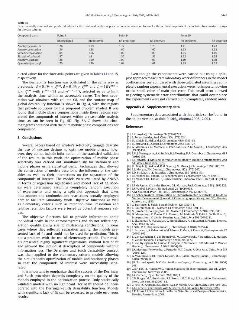
Ametryn/cyanazine 1.26 1.29 1.77 1.75 1.41 1.43Ametryn/symazine 1.36 1.38 1.60 1.60 1.53 1.52S 1.05S 1.50A 1.09C 1.64

dr

pytrgtfatmc

5

teosmtacieoiharu

iacsneaiwtsr

amvpwr

[

[

[[[[

[[[

[

[[

[

[

[

[

[

[

[

imazine/cyanazine 1.05 1.06imazine/carbaryl 1.87 1.81metryn/carbaryl 1.28 1.29yanazine/carbaryl 1.70 1.70

icted values for the three axial points are given in Tables 14 and 15,espectively.

The desirability function was postulated in the same way asreviously: d = 0 if yi < ymin

i, d = 0 if yi > ymax

iand di = 1 if ymin

i≤

ˆ i ≤ ymaxi

with yimin = 1.1 and yi

max = 1.7, selected so as to limithe analysis time within an acceptable range. The best sepa-ation was obtained with column C8, and the contour map oflobal desirability function is shown in Fig. 4, with the regionshat provide solutions for the proposed problem shaded. It wasound that mobile phase compositions inside these regions sep-rated the compounds of interest within a reasonable analysisime, as can be seen in Fig. 5D. Fig. 5A–C shows the chro-

atograms obtained with the pure mobile phase compositions, foromparison.

. Conclusions

Several papers based on Snyder’s selectivity triangle describehe use of mixture designs to optimize mobile phases, how-ver, they do not include information on the statistical validationf the results. In this work, the optimization of mobile phaseelectivity was carried out simultaneously for stationary andobile phases using statistical design techniques that allowed

he construction of models describing the influence of the vari-bles as well as their interactions on the separation of theompounds of interest. The models were evaluated by ANOVAn terms of regression significance and model lack of fit. Mod-ls were determined assuming completely random executionf experiments and using a split-plot approach that takesnto account the randomization restrictions actually employedere to facilitate laboratory work. Objective functions as wells elementary criteria such as retention time, resolution andelative retention factors were tested as potential response val-es.

The objective functions fail to provide information aboutndividual peaks in the chromatograms and do not reflect sep-ration quality giving rise to misleading conclusions. In someases where they reflected separation quality, the models pre-ented lack of fit and could not be used for prediction. This isot a problem with the use of elementary criteria. Their mod-ls presented highly significant regressions, without lack of fitnd allowed the individual description of compounds withoutnformation loss. The Derringer and Suich desirability conceptas then applied to the elementary criteria models allowing

he simultaneous optimization of mobile and stationary phaseso that the compounds of interest were successfully sepa-ated.

It is important to emphasize that the success of the Derringernd Suich procedure depends completely on the quality of the

odels employed in the optimization process. Only statistically

alidated models with no significant lack of fit should be incor-orated into the Derringer–Suich desirability function. Modelsith significant lack of fit can be expected to provide erroneous

esults.

[

[[[

1.09 1.05 1.091.52 1.32 1.321.03 1.19 1.181.67 1.29 1.22

Even though the experiments were carried out using a split-plot approach to facilitate laboratory work differences in the modelcoefficient errors, compared with those calculated assuming a com-pletely random experimental execution, were not important owingto the small value of main-plot error. This small error allowedneglecting systematic error contributions that could occur sincethe experiments were not carried out in completely random order.

Appendix A. Supplementary data

Supplementary data associated with this article can be found, inthe online version, at doi:10.1016/j.chroma.2008.12.093.

References

[1] L.R. Snyder, J. Chromatogr. 92 (1974) 223.[2] L. Rohrschneider, Anal. Chem. 45 (1973) 1241.[3] J.L. Glajch, J.J. Kirkland, J. Chromatogr. 485 (1989) 51.[4] J.J. Kirkland, J.L. Glajch, J. Chromatogr. 255 (1983) 27.[5] G. Mazerolles, D. Mathieu, R. Phan-Tan-Luu, A.M. Siouffi, J. Chromatogr. 485

(1989) 433.[6] P.M.J. Coenegracht, A.K. Smilde, H.J. Meeting, D.A. Doornbos, J. Chromatogr. 485

(1989) 195.[7] L.R. Snyder, J.J. Kirkland, Introduction to Modern Liquid Chromatography, 2nd

ed., Wiley, New York, 1979.[8] J.L. Glajch, J.J. Kirkland, K.M. Squire, J.M. Minor, J. Chromatogr. 199 (1980) 57.[9] S.L. Morgan, S.N. Deming, J. Chromatogr. 112 (1975) 267.10] T.D. Schlabach, J.L. Excoffier, J. Chromatogr. 439 (1988) 173.

[11] P.F. Vanbel, B.L. Tilquin, P.J. Schoenmakers, J. Chromatogr. A 697 (1995) 3.12] P.F. Vanbel, B.L. Tilquin, P.J. Schoenmakers, Chemom. Intell. Lab. Syst. 35 (1996)

67.13] P.F. de Aguiar, Y. Vander Heyden, D.L. Massart, Anal. Chim. Acta 348 (1997) 223.14] P.F. Vanbel, J. Pharm. Biomed. Anal. 21 (1999) 603.15] A.M. Siouffi, R. Phan-Tan-Luu, J. Chromatogr. A 892 (2000) 75.16] P.J. Schoenmakers, Optimization of Chromatographic Selectivity. A Guide to

Method Development (Journal of Chromatography Library, vol. 35), Elsevier,Amsterdam, 1986.

[17] G. Derringer, R. Suich, J. Qual. Technol. 12 (1980) 14.18] B. Bourguignon, D.L. Massart, J. Chromatogr. 586 (1991) 11.19] M. Jimidar, B. Bourguignon, D.L. Massart, J. Chromatogr. A 740 (1996) 109.20] D. Mangelings, C. Perrin, D.L. Massart, M. Maftouh, S. Eeltink, W.Th. Kok, P.J.

Schoenmakers, Y. Vander Heyden, Anal. Chim. Acta 509 (2004) 11.21] T. Sivakumar, R. Manavalan, C. Muralidharan, K. Valliappan, J. Pharm. Biomed.

Anal. 19 (2007) 29.22] F. Safa, M.R. Hadjmohammadi, J. Chromatogr. A 1078 (2005) 42.23] S. Furlanetto, S. Orlandini, A.M. Marras, P. Mura, S. Pinzauti, Electrophoresis 27

(2006) 805.24] E. Van Gyseghem, S. Van Hemelryck, M. Daszykowski, F. Questier, D.L. Massart,

Y. Vander Heyden, J. Chromatogr. A 988 (2003) 77.25] E. Van Gyseghem, M. Jimidar, R. Sneyers, E. Verhoeven, D.D. Massart, Y. Vander

Heyden, J. Chromatogr. A 1042 (2004) 69.26] J.A. Martinez-Pontevedra, L. Pensado, M.C. Casais, R. Cela, Anal. Chim. Acta 515

(2004) 127.27] G. Vivó-Truyols, J.R. Torres-Lapasió, M.C. Garcia-Alvarez-Coque, J. Chromatogr.

A 876 (2000) 17.28] J.R. Torres-Lapasió, M.C. Garcia-Alvarez-Coque, J. Chromatogr. A 1120 (2006)

308.29] G.E.P. Box, J.S. Hunter, W.G. Hunter, Statistics for Experimenters, 2nd ed., Wiley-

Interscience, New York, 2005.30] J.A. Cornell, J. Qual. Technol. 20 (1988) 1.

31] C.N. Borges, M.C. Breitkreitz, R.E. Bruns, L.M.C. Silva, I.S. Scarminio, Chemometr.

Intell. Lab. Syst. 89 (2007) 82.32] C. Reis, J.C. Andrade, R.E. Bruns, R.C.C.P. Moran, Anal. Chim. Acta 369 (1998) 269.33] J.A. Cornell, Experiments with Mixtures, 2nd ed., Wiley, New York, 1990.34] R.E. Bruns, I.S. Scarminio, B. de Barros Neto, Statistical Design – Chemometrics,

Elsevier, Amsterdam, 2006.