HEAPS, KOSLOSKY, SIDLE, LEVINE: IMAGE FUSION USING GMMS 1

Image FusionUsing Gaussian Mixture Models

Katie Heaps1

heaps006@umn.edu

Josh Koslosky1

kosl0052@umn.edu

Glenn Sidle2

sidleg@duq.edu

Stacey Levine2

sel@mathcs.duq.edu

1 Department of MathematicsUniversity of MinnesotaMinneapolis, MN, USA

2 Department of Mathematics andComputer ScienceDuquesne UniversityPittsburgh, PA, USA

AbstractIn recent years, a number of works have demonstrated that processing images using

patch-based features provides more robust results than their pixel based counterparts. Acontributing factor to their success is that image patches can be expressed sparsely inappropriately defined dictionaries, and these dictionaries can be tuned to a variety of ap-plications. Yu, Sapiro and Mallat [24] demonstrated that estimating image patches frommultivariate Gaussians is equivalent to finding sparse representations in a structured over-complete PCA-based dictionary. Furthermore, their model reduces to a straightforwardpiecewise linear estimator (PLE). In this work we show how a similar PLE can be for-mulated to fuse images with various linear degradations and different levels of additivenoise. Furthermore, the solution can be interpreted as a sparse patch-based representa-tion in an appropriately defined PCA dictionary. The model can also be adapted to betterpreserve edges and increase PSNR by adapting the level of smoothing to each local patch.

1 IntroductionIn recent years, a number of successful models have been developed for processing im-ages using patch-based features (see e.g. [10] and references therein). Often critical to thisapproach is that natural image patches can be expressed sparsely in appropriately defineddictionaries which can be tuned to a variety of applications.

In this work we consider the following image degradation model. Suppose an image fhas undergone some linear degradation U (e.g. linear blur, pixel loss, subsampling, etc.)and is corrupted by additive noise w ∼ N (0,σ2). Then the observed, degraded data canbe written as y = U f + w. The goal is to recover f from y. Decomposing f into overlap-ping

√n×√

n vectorized patches fi ∈ Rn for i = 1.., I and noting that each patch may haveundergone a unique linear degradation Ui and contains different additive noise wi we canexpress the degraded image patches as yi = Ui fi + wi for i = 1, .., I. Recovering f from ynow becomes the problem of recovering fi from yi and rebuilding f from the clean patches{ fi}I

i=1.

c© 2013. The copyright of this document resides with its authors.It may be distributed unchanged freely in print or electronic forms.

2 HEAPS, KOSLOSKY, SIDLE, LEVINE: IMAGE FUSION USING GMMS

The sparse dictionary model for solving this problem can be formulated as follows [9].Given a dictionary D ∈ Rn×k where n ≤ k (D can either be fixed or learned from the data),for each degraded image patch, yi, one wishes to find a sparse coefficient vector αi ∈Rk suchthat fi ≈ Dαi. The optimal coefficients are typically recovered by solving

α̂i = arg minα∈Rk

λ ||α||p +12||UiDα− yi||22 (1)

where p = 0 or 1 is most commonly used for inducing sparsity, and λ > 0 is fixed anddetermined by the noise level.

In [24], the authors proposed a technique for solving generalized inverse problems usinga piecewise linear estimator (PLE) that selects the best patch approximation from a fixednumber of multivariate Gaussians. The authors demonstrate this approach performs betterthan (1) as well as other state-of-the-art approaches for a number of linear degradations. Ofparticular note is that the coherence of the dictionary is no longer a problem for challengingapplications such as deblurring and zooming.

In this work we propose a model for fusing multiple images, y1, ...,yJ of the same field ofview into a single image f with optimal properties from each one. Image fusion is used in anumber of applications where a single image is desired from multi-channel data that retainsdesirable information from each channel. This is a problem in military and medical applica-tions e.g [13, 15, 19], images with different depths of focus e.g. [12, 16, 21], panchromaticzooming of satellite images e.g. [2, 26], simultaneous image fusion with super-resolution[23], and fusing noisy image bursts [4], blurry image stacks [18], or noisy/blurry pairs e.g.[3, 25], an application of particular interest in photography. Due to space limitations, anexhaustive list of applications would be impossible to include here. But these are a few ex-amples of the wide range of applications that a generic image fusion model may be able toaddress.

To this end, we propose a general framework for fusing a set of degraded images y1, ...,yJ

that may have different levels additive noise, w1, ...,wJ , as well as different linear degrada-tions, U1, ...,UJ . We use a patch based approach given its robustness as well as flexibility. Asimple extension of (1) would be to solve for image patches fi ≈ Dα̂i, where

α̂i = arg minα∈Rk||α||p +

J

∑j=1

12λ j ||U

ji Dα− y j

i ||22. (2)

However, whether D is a fixed or learned dictionary, (2) has some inherent challenges. Ifp = 0, although this non-convex functional can be solved using a pursuit algorithm [21,22], these pursuit algorithms generally require an ordering of the most influential dictionaryelements for a given patch f . However, the most influential dictionary elements may varyacross the multi-channel data, presenting some challenges. If p = 1, certain common lineardegradation operators U (e.g. subsampling and convolution) do not guarantee the RestrictiveIsometry Property [5, 8] which is typically used to guarantee sparsity when minimizing thel1 norm. It is possible to construct dictionaries that can still handle these issues for a singledegradation operator, but this becomes quite restrictive when trying to fuse images withdifferent degradations.

We show that the general approach for solving inverse problems in [24] has a naturalextension to the image fusion problem which avoids some of the above mentioned concerns.The first primary benefit is its ease in formulation and implementation. There are no param-eters to be tweaked, and it has a simple closed form solution. The second benefit is that as

HEAPS, KOSLOSKY, SIDLE, LEVINE: IMAGE FUSION USING GMMS 3

shown in [24], it outperforms comparable methods when applied to single image restoration,in particular, when restoring low resolution or blurry images. Finally, it naturally lends itselfto simple modifications that can assist in e.g. edge enhancement by weighting a single regiondifferently across multiple images, depending on the level of detail and degradation in thegiven channel.

The rest of the paper is organized as follows. In section 2 we describe the model andits implementation. In section 3 we describe how solving the GMM based fusion model isequivalent to solving a sparse dictionary representation problem. Results are contained insection 4.

2 The Basic Image Fusion Model

2.1 BackgroundYu Sapiro and Mallat [24] proposed a simple yet powerful algorithm for solving the follow-ing general inverse problem: recover a ’true image’ f from a degraded image y = U f + wwhere U is a linear operator and w is additive Gaussian noise. The linear degradation U canbe the identity operator (in the case of denoising) or may represent common degradationssuch as pixel loss (masking), blurring, or subsampling. This problem can be particularlychallenging when using a dictionary based approach since the coherence of the dictionarywith respect to the degradation operator U plays a critical role in successful signal recovery.The authors in [24] proposed a probabilistic based approach using Gaussian Mixture Mod-els aimed to solve inverse problems with a variety of degradation operators, U , which theydemonstrate is comparable to or improves upon state of the art techniques.

The degraded image, y, is decomposed into vectorized√

n×√

n blocks, yi = Ui fi + wi,for i = 1, ..., I. The idea is that these image patches can be described by a mixture of mul-tivariate Gaussian distributions with appropriately defined means and covariance matrices.Assuming we are given K multivariate Gaussians {N (µk,Σk)}1≤k≤K parametrized by theirmeans µk ∈ Rn and covariance matrices Σk ∈ Rn×n, each reconstructed patch fi is drawnfrom one of these Gaussians (which are equally likely) for some ki ∈ {i, ...,K} according tothe probability density function

p( fi) =1

(2π)N/2|Σki |1/2 exp(−1

2( fi−µki)

TΣ−1ki

( fi−µki))

. (3)

Finding the optimal image patches becomes a non-convex optimization problem, but the au-thors in [24] proposed a maximum a posteriori expectation-maximization algorithm (MAP-EM) for solving this problem.

In this work, we demonstrate how this approach can be used to solve the image fusionproblem in which any given number of images of the same field of view can be fused intoa single image, retaining optimal properties from each one. We are not aware of other algo-rithms that easily adapt to the general fusion problem when variable linear degradations areinvolved. To this end, we assume we are given J degraded images of the same field of view,

y1 = U1 f +w1, ..., yJ = UJ f +wJ .

For simplicity we assume the images are perfectly aligned, although the operators U1, ...,UJ

may be different. Perfect alignment is a strong assumption, but our intent to propose ageneral framework. We thus refer the reader to a number of existing image registrationalgorithms (e.g. [1, 6, 14, 17]) that can be used for specialized applications.

4 HEAPS, KOSLOSKY, SIDLE, LEVINE: IMAGE FUSION USING GMMS

2.2 MAP-EM Algorithm2.2.1 Signal Estimation and Model Selection (E-step)

We assume that the number of Gaussians, K and their parameters {(µk,Σk)}1≤k≤K are known(we discuss the initialization in section 2.3) and estimate the signal patches by maximizingthe log a-posteriori probability, log p( fi|y1

i , ...,yJi ,Σk) for each k, as given in (3). We assume

that fi ∼N (0, Σ̂k) and w ji ∼N (0,σ2

j Id) for j = 1, ...,J where Id is the identity matrix. Foreach patch i = 1, ..., I, we wish to maximize the following log a-posteriori likelihood, whichusing Bayes rule is

( f̂i, k̂i) = argmaxf ,k

log p( f |y1i , ...,y

Ji , Σ̂k)

=argmaxf ,k

J

∑j=1

log p(y ji | fi, Σ̂k)+ log p( fi|Σ̂k)

=argminf ,k

J

∑j=1

(1

σ2j||Ui f − y j

i ||2

)+ f T

Σ̂−1k f + log |Σ̂k| (4)

For each fixed k in (4), a simple linear filter gives the minimizer with respect to f as

f ki =

J

∑j=1

W jk,iy

ji where W j

k,i = Σ̂k

(J

∑l=1

1σ2

l(U l

i )TU l

i Σ̂k + Id

)−1

(U ji )T . (5)

Then for i = 1, ..., I, the solution of (4) is given by the pair

f̂i = f k̂ii where k̂i = argmin

k∈{1,...,K}

J

∑j=1

(1

σ2j||Ui f k

i − y ji ||

2

)+( f k

i )TΣ̂−1k f k

i + log |Σ̂k|. (6)

In practice K is small (we use K = 19), so k̂i in (6) is found by simply calculating the energyfor each k = 1, ...,K and finding the argument that yields the smallest value. Although eachpatch is estimated from a single Gaussian, the patches are overlapping (patches centered atevery pixel in the image are used) and the overlapping patches are averaged at each locationto produce the final result, so each pixel will typically contain a mixture of Gaussians.

2.2.2 Gaussian Model Parameter Estimation (M-Step)

Once the model selection k̂i and signal estimation f̂i are known for each patch, setting Ck ={i|k̂i = k} for k = 1, ...,K, the new Gaussian parameters are computed by

µ̂k =1|Ck| ∑

i∈Ck

f̂i and Σ̂k =1|Ck| ∑

i∈Ck

( f̂i− µ̂k)T ( f̂i− µ̂k) (7)

which satisfy (µ̂k, Σ̂k) = argmaxµk,Σk p({ f̂i}i∈Ck |µk,Σk).

2.3 InitializationThe initialization of the Gaussian parameters µk and Σk are critical to the success of themodel. We follow the initialization in [24] which is based on the observation that in manylearned dictionaries, the dominant patches looked like edge elements of a fixed orientation.

HEAPS, KOSLOSKY, SIDLE, LEVINE: IMAGE FUSION USING GMMS 5

Initialization:

1. Eighteen binary straight edge images of fixed orientations at 10o increments from 0o

to 170o were generated.

2. For each of the 18 edge images,

(a) the edge image is randomly sampled until a nonsingular covariance matrix canbe formed from the data.

(b) the dominant eigenvector of the covariance matrix (which is almost DC) is setto be a constant and Gram-Schmidt is used to guarantee the PCA basis is or-thonormal. Then for k = 1, ...,18, Σk = BkΛkBt

k, where Bk = [b1k . . .bn

k ] is theorthonormal PCA basis and Λk = diag(λ 1

k , ...,λ nk ) is the diagonal matrix of as-

sociated (decreasing) eigenvalues. For simplicity, µk = 0.

3. A 19th Gaussian was created based on the Discrete Cosine Transform to allow formore variability in the textures, yielding K = 19 total Gaussians.

4. If the fusion involves a blurring operator for any y j, j = 1, ...,J, a hierarchical basis isused incorporating a second layer of varying positions for each of the directional PCAbases described above. We refer the reader to [24] Section VII.A for more details.

Remark: An alternate initialization derived from natural images was recently proposed [20]for a SURE (Stein’s Unbiased Risk Estimator) guided Piecewise Linear Estimator (S-PLE).The model in [20] is intended for denoising, for which it is both quite successful and math-ematically well motivated. To the best of our knowledge, it has not yet been extended toimage data that has undergone linear degradations, but this opens up a new line of researchin the consideration of alternate initializations, particularly for specialized applications.

3 Sparse Patch-Based ModelingThe MAP-EM algorithm described in section 2.2 has a direct sparse modeling interpretation.A straightforward computation shows that the solution in (5) is precisely f k

i = Bkiaki where

aki = arg min

a∈Rn

(J

∑j=1

1σ2

j||U j

i Bka− y ji ||

2 +N

∑m=1

|a[m]|2

λ km

). (8)

Here Bk is the orthonormal PCA basis diagonalizing the covariance matrix Σk and the λ km

are the corresponding eigenvalues in decreasing order. Although the second term in (8) isa weighted l2 norm, it favors dominant eigenvectors and the eigenvalues rapidly decrease inmagnitude [24], thus inducing sparsity. Furthermore, the PCA basis Bk and the eigenvaluesincorporate information from the data in the M-Step, so this model promotes collaborativefiltering in which the dictionary is learned from the data.

Dictionary construction is particularly important when allowing for linear degradationsUi since here we assume yi =UiBkai +wi, and while each of the dictionaries Bk might satisfy‘good’ dictionary properties (e.g. sparsity, recoverability, and stability [24]), UiBk might not.For example, if Bk contained the atoms b1 = (1,1,1, ...1)T and b2 = (1,−1,1,−1, ...,−1)T

and Ui were a subsampling operator, then Uib1 = (1,1,1, ...1)T = Uib2 and stability wouldbe violated. In this case it is equally likely that a sparsity inducing model such as (1) wouldchoose b2 as b1 to best represent a smooth region, which could be disastrous for the finalresult. The initialization and parameter estimation described in section 2 avoid this problem.

6 HEAPS, KOSLOSKY, SIDLE, LEVINE: IMAGE FUSION USING GMMS

(a) (b) (c) (d)

Figure 1: (a), (b), (c): images of the same field of view with random 80% masking, (d): thefinal fused result using the proposed approach.

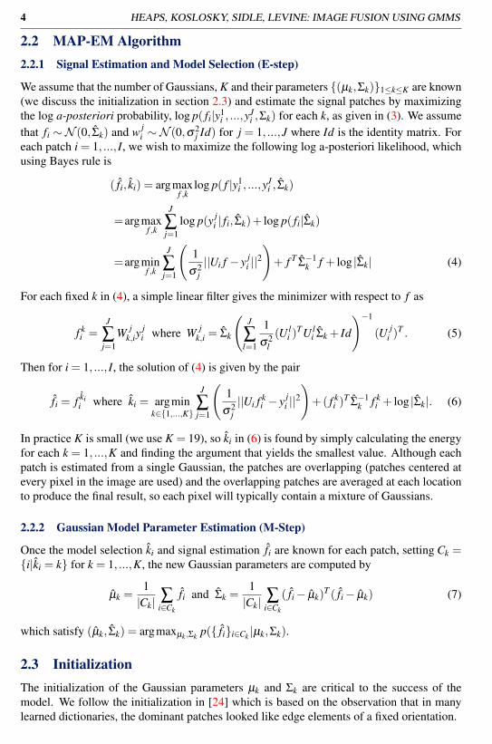
Figure 2: Left: Result of running the single image MAP-EM algorithm on the masked imagefrom figure 1(a) only, PSNR = 26.1547; Middle: Result of running the single image MAP-EM algorithm on the average of the masked images in figure 1, PSNR = 30.8393; Right:Result of the proposed fusion model (close up the result in figure 1), PSNR = 32.5033.

4 Results

We tested the fusion model on several sets of images involving varying noise levels and lineardegradations. Our patch sizes are all 8×8, so n = 64. In [24] the authors provide a numberof examples that confirm that except in the case of denoising (where BM3D [7] still seemsto outperform all comparable models), the single image PLE using the MAP-EM algorithmgenerally provided state-of-the art results for difficult problems involving linear degrada-tions, inlcuding deblurring and subsampling. Given the range of applied fusion problems,we provide here several examples to demonstrate the ease and success of the model for fus-ing image sets with a variety of degradations. Our intent is to provide a proof of concept,opening the door to more specialized applications by the user. For simplicity we assume theimages are perfectly aligned, although many real world problems do not afford this luxury.In the latter case, one could choose to preprocess the data with an existing image warpingalgorithm, e.g. [1, 6, 14, 17].

Figure 1 contains a set of images with varying degrees of masking and the final fused

HEAPS, KOSLOSKY, SIDLE, LEVINE: IMAGE FUSION USING GMMS 7

Table 1: PSNR: PLE [24] -vs- PLE with adaptive smoothing (9)-(10); tests performed on thestandard image database with noise level σ=25; the average increase in PSNR is 0.42.

Image noisy image GMM [24] GMM+AS (9)-(10)Barbara 20.1721 27.6023 28.0768Blonde 20.1664 28.9708 29.2502Boat 20.201 25.277 26.1944Bridge 20.1607 25.1989 25.6419Brunette 20.1696 33.78 33.8809Cameraman 20.1783 31.4219 31.5926Fair 20.1702 28.3473 28.6918Lena 20.1711 30.8052 31.0635Oldies 20.1787 28.244 28.5609Peppers 20.1347 27.515 28.1031Plane 20.1806 29.4183 30.1749

result using the proposed model. In figure 2, we compare the result of recovering the im-age from a single masked image using the model in [24], the result of simply averagingthe ’known pixels’ from the masked images in figures 1(a-c) and running the single imagepiecewise linear estimator from [24], and the result using the fusion model proposed here.We note both the increase in PSNR, as well as visual improvements which include smootherhomogeneous regions while preserving edges and textures.

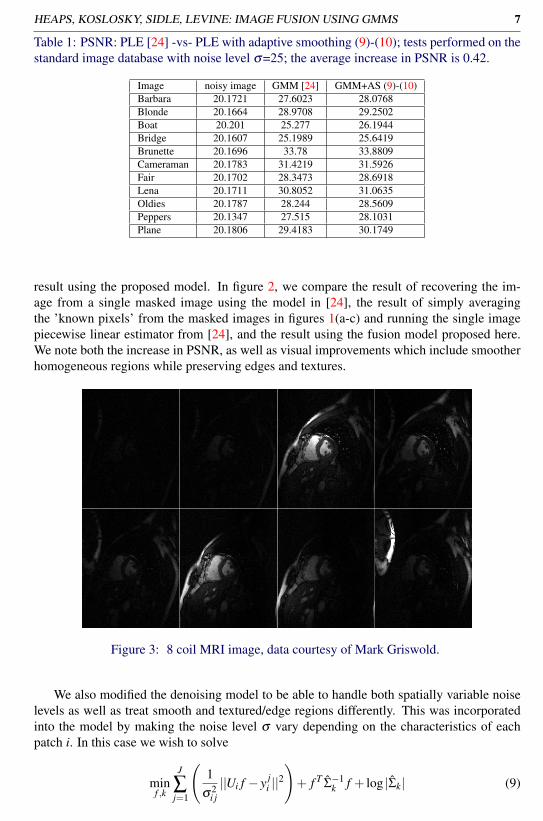
Figure 3: 8 coil MRI image, data courtesy of Mark Griswold.

We also modified the denoising model to be able to handle both spatially variable noiselevels as well as treat smooth and textured/edge regions differently. This was incorporatedinto the model by making the noise level σ vary depending on the characteristics of eachpatch i. In this case we wish to solve

minf ,k

J

∑j=1

(1

σ2i j||Ui f − y j

i ||2

)+ f T

Σ̂−1k f + log |Σ̂k| (9)

8 HEAPS, KOSLOSKY, SIDLE, LEVINE: IMAGE FUSION USING GMMS

(a) (b)

Figure 4: Results of fusing the 8 coils in figure 3: (a) Result from [11], (b) Result from theproposed method.

where σi j is either the estimated noise level in image j at patch i, or is weighted dependingon edge information, such as

σi j = σ j×(

11+ k|∇Gτ ∗ yi|2

+0.5)

. (10)

Here σ j is the estimated noise level for the entire image, Gτ is a Gaussian of standard de-viation τ and k > 0 is a positive parameter. Note that in patches containing high gradientinformation (likely edges), |∇Gτ ∗ yi| will be large so the so the local noise level σi j ≈

σ j2 ,

yielding less smoothing. In patches with low variations in the gradient, likely smooth re-gions, the local noise level σi j ≈

3σ j2 . In our experiments we set τ = .07 (for a noise level of

σ j = 25) and k = 0.0075 (for images with intensity in the range [0,255]). These parameterscan be locally optimized, but we found this worked fairly well in getting a general improve-ment on the standard image database (see table 1). It is important to point out that this modeldoes not necessarily give state of the art results with respect to denoising alone (for exam-ple, BM3D [7] consistantly achieves better results). The power in the proposed model is thegeneral framework in which images with multiple degradations can be combined.

We also tested the proposed fusion model on an 8 coil parallel MRI image dataset. Thefinal fused result should retain fine features (e.g. vessels in the lung) while not introducingspurious features. Typical variational denoising methods can lead to the oversmoothing offine features for this kind of data, and the more detail preserving techniques often lead tostaircasing and thus unwanted artifacts. The noise level is uniform throughout a single coil,but varies between coils. A simple application of our fusion model preserved fine detailwhile attenuating noise.

Our final example is the fusion of a noisy-blurry pair, an application that could arise whenimages with varying exposure times are combined into a single image. Noisy and blurryversions of the color image in figure 5 were processed separately as well as fused using theproposed model to obtain a result that incorporated information from both images in the set(color channels were processed separately). The intensity cross sections in figure 6 weretypical for flat and detailed regions in the image, and demonstrate how the model readilyextracts the relevant information from the images being fused; the flat regions are closer tothe original color than denoising alone, and the details are more accurately preserved thandeblurring alone. Figure 7 contains a close up view of a grassy region below the plane to

HEAPS, KOSLOSKY, SIDLE, LEVINE: IMAGE FUSION USING GMMS 9

(a) (b) (c)

(d) (e) (f)

Figure 5: First row: (a) blurry image, PSNR=27.5454 (b) noisy image, PSNR=29.2852, (c)original clean image; Bottom row: (d) deblurred image only, PSNR=31.3776, (e) denoisedimage only, PSNR=33.4498, (f) result of fusing the noisy/blurry pair; that is, both imagesfrom the first row, PSNR=35.7534.)

(a) (b)

Figure 6: Typical cross-sections of the magnitude of the intensity: (a) flat region of thesky (b): detailed region across the lettering on the plane (blue=original image, green=fusedresult, red=denoised only, magenta=deblurred only).

(a) (b) (c) (d)

Figure 7: Close up of a typical textured region: (a) result of deblurring the image in figure5(a); (b) result of denoising the image in figure 5(b); (c) result of the proposed fusion model;(d) the original clean image

10 HEAPS, KOSLOSKY, SIDLE, LEVINE: IMAGE FUSION USING GMMS

illustrate the level of detail preserved in the textured regions of the fused image.We should note that a number of successful models exist for specialized problems in

image fusion. Our intent is to propose a simple, flexible, and general framework for fusingimages containing noise and linear degradations, and illustrate the behavior and potential offusing images in this framework.

AcknowledgementsWe would like to thank Guoshen Yu, Guillermo Sapiro and John Kern for their helpful dis-cussions. The last author was funded in part by NSF-DMS #0915219.

References[1] http://www.revisionfx.com/products/twixtor/.

[2] Coloma Ballester, Vicent Caselles, Laura Igual, Joan Verdera, and Bernard Rougé. Avariational model for p+xs image fusion. International Journal of Computer Vision, 69(1):43–58, 2006.

[3] M. Bertalmio and S. Levine. Variational approach for the fusion of exposure bracketedpairs. Image Processing, IEEE Transactions on, 22(2):712–723, 2013. ISSN 1057-7149.

[4] A. Buades, Y. Lou, J. M. Morel, and Z. Tang. A note on multi-image denoising.Proceedings of the International Workshop on Local and Non-Local Approximation(LNLA) in Image Processing, August 2009.

[5] E.J. Candes, J. Romberg, and T. Tao. Robust uncertainty principles: exact signal re-construction from highly incomplete frequency information. Information Theory, IEEETransactions on, 52(2):489–509, 2006.

[6] I.J. Cox, S.L. Hingorani, S.B. Rao, and B.M. Maggs. A maximum likelihood stereoalgorithm. Computer vision and image understanding, 63(3):542–567, 1996.

[7] K. Dabov, A. Foi, V. Katkovnik, and K. Egiazarian. Image denoising by sparse 3-dtransform-domain collaborative filtering. Image Processing, IEEE Transactions on, 16(8):2080–2095, 2007.

[8] D.L. Donoho. Compressed sensing. Information Theory, IEEE Transactions on, 52(4):1289–1306, 2006.

[9] M. Elad, M.A.T. Figueiredo, and Yi Ma. On the role of sparse and redundant represen-tations in image processing. Proceedings of the IEEE, 98(6):972 –982, June 2010.

[10] Michael Elad. Sparse and redundant representation modeling - what next? SignalProcessing Letters, IEEE, 12(12):922 – 928, 2012.

[11] M. Griswold, D. Walsh, R. Heidemann, A. Haase, and P. Jakob. The Use of an AdaptiveReconstruction for Array Coil Sensitivity Mapping and Intensity Normalization. InProc. Intl. Soc. Mag. Reson. Med., volume 10. ISMRM, 2002.

HEAPS, KOSLOSKY, SIDLE, LEVINE: IMAGE FUSION USING GMMS 11

[12] Shutao Li, James T. Kwok, and Yaonan Wang. Multifocus image fusion using artificialneural networks. Pattern Recogn. Lett., 23(8):985–997, June 2002.

[13] N. Mitianoudis and T. Stathaki. Adaptive image fusion using ica bases. In Acoustics,Speech and Signal Processing, 2006. ICASSP 2006 Proceedings. 2006 IEEE Interna-tional Conference on, volume 2, pages II–II, 2006.

[14] N. Papenberg, A. Bruhn, T. Brox, S. Didas, and J. Weickert. Highly accurate optic flowcomputation with theoretically justified warping. International Journal of ComputerVision, 67(2):141–158, 2006.

[15] Xiao-Bo Qu, Guo-Fu Xie, Jing-Wen Yan, Zi-Qian Zhu, and Ben-Gang Chen. Imagefusion algorithm based on neighbors and cousins information in nonsubsampled con-tourlet transform domain. In Wavelet Analysis and Pattern Recognition, 2007. ICWAPR’07. International Conference on, volume 4, pages 1797–1802, 2007.

[16] R. Redondo, F. Šroubek, S. Fischer, and G. Cristóbal. Multifocus image fusion usingthe log-gabor transform and a multisize windows technique. Inf. Fusion, 10(2):163–171, April 2009.

[17] Y. Shinagawa and T.L. Kunii. Unconstrained automatic image matching using mul-tiresolutional critical-point filters. IEEE Transactions on Pattern Analysis and MachineIntelligence, pages 994–1010, 1998.

[18] F. Sroubek and J. Flusser. Multichannel Blind Deconvolution of Spatially MisalignedImages. IEEE Transactions on Image Processing, 14(7):874–883, 2005.

[19] Tao Wan, N. Canagarajah, and A. Achim. Compressive image fusion. In Image Pro-cessing, 2008. ICIP 2008. 15th IEEE International Conference on, pages 1308–1311,2008.

[20] Y.-Q. Wang and J.M. Morel. Sure guided gaussian mixture image denoising. HAL:hal-00785334, version 1, 2013.

[21] Bin Yang and Shutao Li. Multifocus image fusion and restoration with sparse repre-sentation. Instrumentation and Measurement, IEEE Transactions on, 59(4):884–892,2010.

[22] Bin Yang and Shutao Li. Pixel-level image fusion with simultaneous orthogonal match-ing pursuit. Inf. Fusion, 13(1):10–19, January 2012.

[23] Haitao Yin, Shutao Li, and Leyuan Fang. Simultaneous image fusion and super-resolution using sparse representation. Information Fusion, 14(3):229 – 240, 2013.

[24] Guoshen Yu, Guillermo Sapiro, and Stephan Mallat. Solving inverse problems withpiecewise linear estimators: From gaussian mixture models to structured sparsity. IEEETrans. Image Process., 21(5):2481– 2499, 2012.

[25] Lu Yuan, Jian Sun, Long Quan, and Heung-Yeung Shum. Image deblurring withblurred/noisy image pairs. IACM Transactions on Graphics, 26(3):1–10, 2007.

[26] Sheng Zheng, Wen zhong Shi, Jian Liu, and Jinwen Tian. Remote sensing image fusionusing multiscale mapped ls-svm. Geoscience and Remote Sensing, IEEE Transactionson, 46(5):1313–1322, 2008.