Gaussian mixture density modeling of non-Gaussian source for autoregressive process

894 IEEE TRANSACTIONS ON SIGNAL PROCESSING, VOL. 43, NO. 4, APRIL 1995

Gaussian Mixture Density Modeling of Non-Gaussian Source for Autoregressive Process

Yunxin Zhao, Senior Member, IEEE, Xinhua Zhuang, Senior Member, and Sheu-Jen Ting

Abstract- A new approach is taken to model non-Gaussian sources of AR processes using Gaussian mixture densities that are known to be effective for approximating wide varieties of probability distributions. A maximum likelihood estimation algorithm is derived for estimating the AR parameters by solving a generalized normal equation, and a clustering algorithm is used for estimating the parameters of Gaussian mixture density of the source signals. The correlation matrix of the generalized normal equation is not Toeplitz but is symmetric and in general positive definite. Higher order statistics of skewness and kurtosis are used for identifying the source distribution as being Gaussian or non-Gaussian and, consequently, determining the parameter estimation technique between the conventional method and the proposed method. Experiments on non-Gaussian source AR processes demonstrate that under high SNR conditions (SNR > 20 dB), the proposed algorithm outperforms the conventional AR estimation algorithm and the cumulant-based algorithm by an order-of-magnitude reduction of average estimation errors. The proposed algorithm also has very low estimation errors with short data records. Finally, a maximum likelihood prediction method is formulated for non-Gaussian source AR processes that has shown potential in achieving higher efficiency signal coding than linear predictive coding.

I. INTRODUCTION UTOREGRESSIVE (AR) modeling has been an impor- A tant technique for signal analysis such as speech analysis

[ 11, [2]. In previous efforts, the source signal of AR process has been modeled by zero-mean white Gaussian noise, where the AR parameters are solved via the well-known normal equation. In many cases, however, the source distributions could be non- Gaussian, e.g., the distributions are skewed or multimodal. In such cases, more accurate models of the source signal are needed for AR parameter estimation. In the past, several efforts [3]-[5] were reported on the parameter estimation of non- Gaussian AR processes using higher order spectra, where the parameter estimates are theoretically independent of Gaussian noise but lack the property of uniqueness and require long data records.

In this work, a new effort is made to model non-Gaussian sources using Gaussian mixture densities that are known to be effective for approximating wide varieties of probability

Manuscript received September 20, 1993; revised September 14, 1994. The associate editor coordinating the review of this paper and approving it for publication was Prof. Douglas Williams. Y. Zhao is with the Department of Electrical and Computer Engineering,

University of Illinois at Urbana-Champaign, Urbana, IL 61801 USA. X. Zhuang is with the Department of Electrical and Computer Engineering,

University of Missouri, Columbia, MO 6521 1 USA. S.4. Ting is with the Peripheral Devices Corporation, Livermore, CA 94550

USA. IEEE Log Number 9409777.

distributions [6]. A maximum likelihood estimation algorithm is derived for estimating the AR parameters by solving a generalized normal equation, and a clustering algorithm is used for estimating the parameters of Gaussian mixture density of the source signals. The estimation procedure is iterative and actually consists of three steps: inverse filtering for the source signal, Gaussian mixture density parameter estimation, and AR parameter estimation. The correlation matrix of the generalized normal equation is symmetric but not Toeplitz, where the matrix elements are averages of correlation terms weighted by Gaussian likelihoods of mixture components. In general, the correlation matrix is positive definite, which insures the AR parameter estimates to be unique. Higher order statistics of skewness and kurtosis [7] are used for identifying the source distribution as being Gaussian or non-Gaussian. If the distribution is non-Gaussian, the proposed algorithm is used for estimating the AR parameters; otherwise, the conventional method is used. Experiments on non-Gaussian source AR processes demonstrate that under the condition of high signal-to-noise ratio (SNR), the proposed algorithm outperforms the conventional AR estimation algorithm and the cumulant-based algorithm by an order-of-magnitude reduction of average estimation errors. The proposed algorithm also has very low estimation errors with short data records. Finally, a maximum likelihood prediction method is formulated for non- Gaussian source AR processes, where significant reductions of prediction errors are achieved with little extra cost and thus has the potential in achieving a higher efficiency signal coding than the linear predictive coding.

This paper is organized in eight sections. In Sections I1 and 111, the algorithms for AR parameter estimation and for Gaussian mixture density parameter estimation are derived, respectively; the identification of the source distribution is described in Section IV, the overall computational algorithm is summarized in Section V, the prediction problem is formulated and studied in Section VI, the experimental results are given in Section VII, and concluding comments are made in Section VIII.

11. AR PARAMETER ESTIMATION Assume that yn is the output of a causal autoregressive

(AR) model of order P as follows:

1053-587X/95$04.00 0 1995 IEEE

ZHAO et al.: GAUSSIAN MIXTURE DENSITY MODELING OF NON-GAUSSIAN SOURCE

-

895

where yo = y-1 = ... = y - - ( ~ - ~ ) = O,wn is a real, independent, identically distributed (i.i.d) Gaussian or non- Gaussian process. The transfer function of the AR process, i.e., I/A(z), is assumed to be stable with all zeros of A(z ) being inside the unit circle, where

P

i=l

Assume a Gaussian mixture density of size M for the probability density function of the source signal w,, that is

M

(3) m=l

where p;* = (pi, .. . , P M ) , @ = (gi,. .. , U M ) , and cf* = (c1, . . . , C M ) are the means, standard deviations, and weights of Gaussian component densities with c, 2 0 , m = 1,2, . . . , M , cm = 1, and the gm,n’s are the likelihood of w, belonging to the mth Gaussian component density in the mixture, m = 1 , 2 , . . . , M. When M = 1, the Gaussian mixture density is reduced to a single Gaussian density.

Assuming the parameters of the source distribution, i.e. &I, 0t4, and ct* are known, the joint log likelihood of having the N samples of the source signal is given by

N

n=l N M

n=l m=l

where by (1) W n = yn + Er=, a;yn-i, and the joint log likelihood q is therefore a function of AR parameters ur = ( a l , . . . , a p ) . The AR parameters a r are solved by maximizing the log likelihood function q , i.e., iir = argmax,; q. Taking partial derivatives of q with respect to a;, i = 1,2, . . . , P, we arrive at the following equation:

i = 1 , 2 , . - . , P . ( 5 )

FOT simplifying (9, the weighting coefficient cy,,,'^ are defined as

where the weight am,n is seen as the ratio of the likelihood cmgm9, of w, belonging to the mth Gaussian component density to the likelihood p(wn) of w, belonging to the Gaussian mixture density, i.e., the posterior probability that w, be labelled by the mth component of the mixture, and the ratio is inversely weighted by the variance & of the mth Gaussian component density. Note that the weighting

coefficients cy,,, 2 0. Substituting for dq/da;, we arrive at the following equation:

into (5) and solving

P N M

I=1 n=lm=l

n=l m=l m=l n= l

(7)

for i = 1 , 2 , . . . , P . From (7), weighted correlation coefficient Rl,+’s can be

defined for signal sample pairs yn-l and yn-;, where the weighting factor is E$=, cym+, n = 1,2, . . . , N, i.e.

N / M \

Furthermore, weighted bias term Si’s can be defined for signal samples yn-;, where the weighting factor is

cym,n,um,n = 1 ,2 , . . . , N , i.e.

N / M \

Substituting the definitions of Rl,i from (8) and 5’; from (9) into (7), we arrive at the following equation:

which in matrix form is

As seen from (1 l), the AR parameters a? formulated as the maximum likelihood solution can be obtained by solving the system of linear equations.

Certain properties can be derived for the correlation matrix [Rl,,] on the left side of (1 1). From the definition of Rl,, in (8), the correlation coefficients are computed by centering on the successive sample indices n to calculate the weighting factor E:=, am,n, taking the weighted product of two samples yn-l and yn-, with their indices lagging behind n by 1 and i and accumulating such product terms. Since yn-zyn-, = yn-,yn-l, Rl,, = R,,J, and therefore, [Rl,,] is symmetric. Note that because the indices 1 and i are relative to the index n that defines the sample point for calculating the weighting factor Eg=l Rl,, # Rl-,, and therefore, the matrix [Rl,,] is not Toeplitz. Furthermore, if a vector of the observation signal samples is defined by Yn = [ynun-l, yn-p,. . . , yn-p]’

896 IEEE TRANSACTIONS ON SIGNAL PROCESSING, VOL. 43, NO. 4, APRIL 1995

and the weighting factor is denoted by Y~ = a,,,, the correlation matrix can be written as the weighted sum of the outer products of Y,, i.e.

N

n=l

The quadratic term defined by an arbitrary positive vector S = [61,S2, . . . ,6p]’ and the matrix [Rl,i] can be easily shown nonnegative, i.e., S’[Rl,;]S 2 0. Since each Y~ is positive, the correlation matrix {Rl,i] is positive definite if and only if there exist P linearly independent vectors among those N vectors Y1, Y2, . . . , YN, and this positive-definite property insures the uniqueness of the AR parameter estimate from (1 1).

As seen from (1 l) , the estimation of the AR parameters for the case of Gaussian mixture density source is similar to the conventional normal equation but with two differences: one is the weighted correlation matrix [ & , ; I ; the other is the additional bias vector S = [SI, 5’2, . . . , Sp]’. When the source signal distribution is zero-mean Gaussian, i.e., N(0, c2), the conventional normal equation becomes a special case of (1 1) or equivalently (7). As a matter of fact, under such an assumption, the bias term becomes zero since am+p, = 0, and the weighting factor Egzl am,n becomes l/a2, and (7) is then reduced to

which is easily identified as the conventional normal equation. Since the parameter estimation (7) or ( 1 1) subsume the conventional normal equation as a special case, they are referred as the generalized normal equations.

111. GAUSSIAN MIXTURE DENSITY PARAMETER ESTIMATION

A clustering algorithm is used for estimating the parameters of Gaussian mixture density for the source signal. The reason for not directly pursuing a maximum likelihood estimation for the mixture density parameters is that the technique may yield meaningless singular solutions when no constraints are put on the variance terms of the Gaussian densities [6]. Assuming M mixture components, then each Gaussian component supposes to produce a subset of the source signal samples that cluster around its mean. Those M Gaussian clusters may overlap in general. In order to delineate those M clusters, the average variance of the M clusters J = Egzl c,ak is minimized.

Assume that the source signal samples w1, w2, . . . , WN are sorted in the ascending order as ~1 5 u2 5 . . . 5 U N , and the sample v,’s are divided into M nonoverlapping clusters. On the real integer axis, the M clusters are separated by M - 1 indices of the signal samples, i.e., n1 < n2 < . . . < n~4-1, where the left boundary of the first cluster is defined as no = 0, and the right boundary of the Mth cluster is defined as n A r = N . The task of clustering is to find the set of optimal boundary points n; < n; < . . . < nif -1 by which the minimum of the average variance, min J , is attained.

Denoting the interval for the with cluster by (nm-l, n,], where (.I means excluding the left point and including the

right point, the sample mean p,, sample variance a%, and sample weight c, are defined for the cluster as

For a given right boundary point n, of the mth cluster, the minimum cumulative variance w, (n,) can be calculated from the first cluster to the mth cluster over a set of boundary points n l < n 2 < . . . <n,-1 as

m

. aj2(nj-1 + 1, nj). (15)

When m = M , the minimum cumulative variance becomes the minimum average variance, i.e., min J = w M ( n , v ) .

The minimum average variance can be computed recursively via dynamic programming. Denoting the optimal right boundary point of the m-lth cluster by 4,.-1(nm) for each fixed right boundary point n, of the mth cluster, the dynamic- programming clustering procedure proceeds as follows:

Initialization: m = l ,wl(nl) = c l ( l , n1 )a~(1 ,n i ) , 1 < -

Loop: 121 5 N - M + l .

Set m = m+ I , while m 5 M , compute for m 5 n, 5 N - M + m :

&-1(nm) = arg min {wm-l(nm-1) + cm(nm-1+ 1,nm) nn,-l

.g:(nm-l+ 1,nm)>

. g&($m-I(nm) + 1, nm)- wm(nm) =wm-l($m-l(nm)) + cm(&-~(nm) + 1, nm)

(16)

The cluster separation points are backtracked by nLf-l =

4 ~ - i ( n , v ) , . . . , n2-1 = 4,-1 (n;), . . . , nT = 4i(n;). From the intervals separated by the optimal boundary points, the means, variances, and weights are calculated for the individual intervals, and they are taken as the parameters of the Gaussian mixture density. For computational savings in the dynamic programming procedure, the mean and variance of each cluster can be calculated recursively with each single- sample change of cluster size, where the recursive formulas can be easily derived from the definitions of mean and variance in (14).

IV. SOURCE DISTRIBUTION IDENTIFICATION

In general, when specifying a Gaussian mixture density of size M, the above-described clustering algorithm always finds M- 1 separation points for the M clusters, even though the actual signal distribution might be Gaussian. Since using a wrong source distribution could deteriorate the estimation

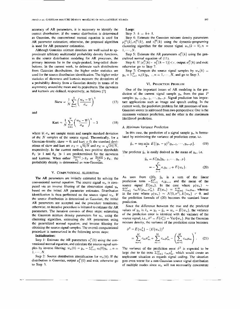
ZHAO et al.: GAUSSIAN MIXTURE DENSITY MODELING OF NON-GAUSSIAN SOURCE 897

accuracy of AR parameters, it is necessary to identify the correct distribution: If the source distribution is determined as Gaussian, the conventional normal equation is used for AR parameter estimation; otherwise, the proposed algorithm is used for AR parameter estimation.

Although Gaussian mixture densities are well suited to ap- proximate arbitrary multimodal probability density functions, in the source distribution modeling for AR processes, the primary interests lie in the single-peaked, long-tailed distributions. In the current work, to delineate such distributions from Gaussian distributions, the higher order statistics are used for the source distribution identification. The higher order statistics of skewness and kurtosis measure the deviations of a probability density from a Gaussian density in terms of its asymmetry around the mean and its peakedness. The skewness and kurtosis are defined, respectively, as follows [7]

3 Skew = - l N ( y) n=l

N

and

where Gl ow are sample mean and sample standard deviation of the N samples of the source signal. Theoretically, for a Gaussian density, skew = 0, and kurt = 0; the standard deviations of skew and kurt are IJS = and CTK = m, respectively. In the current method, two positive thresholds 6s >> 1 and 6 ’ ~ >> 1 are predetermined for the skewness and kurtosis. When either >Os or ,,K > O K > the probability density is determined as non-Gaussian.

V. COMPUTATIONAL ALGORITHM

The AR parameters are initially estimated by solving the conventional normal equation. The source signal w, is computed via an inverse filtering of the observation signal yn based on the initial AR parameter estimates. Distribution identification is then performed on the source signal w,. If the source distribution is determined as Gaussian, the initial AR parameters are accepted and the procedure terminates; otherwise, an iterative procedure is initiated to estimate the AR parameters. The iteration consists of three steps: estimating the Gaussian mixture density parameters for w, using the clustering algorithm, estimating the AR parameters using the generalized normal equation, and inverse filtering for obtaining the source signal samples. The overall computational procedure is summarized in the following seven steps:

Initialization: Step 1: Estimate the AR parameters a r ( 0 ) using the con-

ventional normal equation, and calculate the source signal samples by inverse filtering: wn(0) = y, + CL, a,(0)yn_, ,n =

Step 2: Source distribution identification for UJ,(O): If the distribution is Gaussian, output a r ( 0 ) and exit; otherwise go to Step 3.

1. ... . N .

Loop: Step 3: k = k+ 1. Step 4: Estimate the Gaussian mixture density parameters

pp ( k ) , o;f ( k ) , and c;‘( k ) using the dynamic-programing clustering algorithm for the source signal wn(k - I), n =

Step 5: Estimate the AR parameters u r ( k ) using the gen-

Step 6: If lar(lc) - a r ( k - 1)1 < t, output a r ( k ) and exit:

Step 7: Compute the source signal samples by w n ( k ) =

1, ... , N .

eralized normal equation of (11).

otherwise go to Step 7.

yn + az(k)yn-l,n = l , . ‘ . , N, and go to Step 3.

VI. PREDICTION PROBLEM

One of the important issues of AR modeling is the prediction of the current signal sample y, from the past P samples y,-l1 yn-2,. . . , y,-p. Signal prediction has important applications such as image and speech coding. In the current work, the prediction problem for AR processes of non- Gaussian source is addressed from two perspectives: One is the minimum variance prediction, and the other is the maximum likelihood prediction.

A. Minimum Variance Prediction

In this case, the prediction of a signal sample yn is formulated by minimizing the variance of prediction error, i.e.

The predictor 5, is easily derived as the mean of y,, i.e.

Yn =E{YnlYn-l,...,Y,-P} P

= - aiyn-i + E{w,}. i=l

As seen from (20), G, is a sum of the linear prediction term -Er=, azyn-% and the mean of the source signal E{w,}. In the case where p(w,) N

in the case where p(wn) N N(O,IJ’),E(W,} = 0, and the prediction formula of (20) becomes the standard linear prediction.

Since the difference between the true and the predicted values of yn is 6, = yn - 5, = w, - E{w,}, the variance of the prediction error is identical with the variance of the source signal, i.e., 6’ = E{;:} = Var{w,}. For the Gaussian mixture density, the variance of the prediction error becomes

Em=, M cmN(pm,a2) . E{w,} = c,p,, whereas

8’ = E{lu;} - (E{w,})’ M M

= cmgk + Cmp; - (gl cmpm) ’. (21) m=l m=l

The variance of the prediction error d2 is expected to be large due to the term E:=, c7,p&, which would create an unpleasant situation as regards signal coding. The situation gets even worse for a non-Gaussian source signal distribution of multiple modes since w, will not necessarily concentrate

898 lEEE TRANSACTIONS ON SIGNAL PROCESSING, VOL. 43, NO. 4, APRIL 1995

2 - 1 -0 3989 1 2 3

(a)

where according to the Gaussian mixture density of (3), it reads as

J(YnlYn-1, ’ . . , Y n - P ) hl

m=l

Taking its derivative with respect to yn and setting it to zero, we arrive at the following equation:

Solving the above equation, the estimate of yn is derived as

As seen from (24), the maximum likelihood prediction of yn is the sum of the linear prediction term - E L l aiy,-; and a linear combination of the mixture mean parameters

I , 6 4 2 0 2

(b)

Fig. 1. Two non-Gaussian source distributions: (a) “Non-Gaussian;” (b) “mixture.”

The linear combination term L n ( p ) can be approximated by one of the Gaussian component mean p m , where the difference between L, (p ) and pm is minimized among the indices m = l , . - . , M . Denoting such a mixture component index at time n by m*(n), then m*(n) = argmin, lpm - Ln(p ) l , and (24) can be approximated as

P

d 4 2 0 2

Fig. 2. Gaussian mixture density fitting using the clustering algorithm.

around its mean E{w,}. On the other hand, for the source signal distribution of N(0, 02 ) , the prediction error variance becomes 6’ = a’, which is the same as for the standard linear prediction.

i=l

Note that in the case where p(wn) N M(0, 02), the maximum likelihood predictions of (24) and (26) also reduce to the standard linear prediction.

For evaluating prediction accuracy, the normalized mean- square prediction error E is defined the same as the linear prediction, i.e.

N

B . Maximum Likelihood Prediction

For a maximum likelihood prediction of the signal sample ylL, the objective function is defined as the likelihood of gn,

n=l

As shown by the preliminary experimental result in the next section, the prediction error E for the maximum likelihood prediction is much smaller than that of the minimum variance

ZHAO ct al.: GAUSSIAN MIXTURE DENSITY MODELING OF NON-GAUSSIAN SOURCE 899

N-2048 N-1024 N-512 “256 N-2048 N-1024 N-512 N-256

N-2048 N-1024 N-512 N-256

(C)

N-2048 N-1024 “512 N-256

(d)

Fig. 3. Parameter estimation with variation of data record length on “non-Gaussian” source AR process using the three estimation methods: conventional (U). cumulant-based (0). and proposed (0): SNR = m: the true parameter values are marked by symbols x; the dotted vertical lines mark the standard deviations of the individual parameter estimates: (a) (11: (b) (12: (c) n g : (d) Q.

prediction. Therefore the maximum likelihood prediction may device to become the positive noise 20,: have a potential application in predictive coding.

VII. EXPERIMENTAL RESULTS To evaluate the quality of the proposed algorithm for

estimating the parameters of non-Gaussian AR processes, experiments are conducted on simulated data with the variations of data record length, S N R , and source signal distribution. For comparison, experiments are also carried out using the conventional AR parameter estimation algorithm and the third- cumulant-based estimation algorithm described in [3].

The parameters of the AR process are taken from the example in [3] that defines a fourth-order AR process, where a1 = 0.1, a2 = 0.2238, a3 = 0.0844, a4 = 0.0294. The poles of the AR transfer function are

if e, 2 0 w, = { e, 0 otherwise. (29)

The mean value of w,, -(l/fi), is further subtracted out so that it becomes a zero-mean, non-Gaussian white noise process. Its probability density function can be verified as

l/&), where S(-) denotes the unit-sample function and U ( .) the unit-step function, respectively. The other source distribution is a Gaussian mixture density, with p(20,) - 0.7 * ~v(0.5,0.5~) + 0.3 * N(-1.167, 1.52), which is also a zero-mean, white noise process. The two probability densities are shown in Fig. l(a) and (b), respectively, where the first distribution is referred as “non-Gaussian’’ and the second one “mixture.” It can be clearly seen that the two densi-

p(2On) - (1/2)S(w, + l/G) +N(- ( l /G) , 1) * U ( % +

21,2 = 0.174284 f j0.491668 ties are skewed distributions. The normalized skewness and kurtosis defined in Section IV are 30.07 and 21.64 for “non- Gaussian” and -37.23 and 33.32 for “mixture.” By setting the thresholds 0 s = OK = 5.0 (an empirically determined number), the source distributions were all correctly identified as non-Gaussian. Since both distributions are zero mean for each distribution, the moment and cumulant are identical at

(28)

which all lie inside the unit circle. The source signals w, are generated from two non-Gaussian distributions. One distribution is taken from the example in [3], where a zero-mean, white Gaussian noise e, - N (0, 1) is passed through a nonlinear

23,4 = -0.224283 f j0.240293

IEEE TRANSACTIONS ON SIGNAL PROCESSING, VOL. 43, NO. 4, APRIL 1995

SNR-hl SNRdOdB SNR-lOdB SNRddB

(a)

. . . . . . Bh . . . . . x

4 : : * . . . . .

Fig. 4. length = 2048; the symbol assignments are the same as in Fig. 3: (a) n l : (b) (12: (c ) (13: (d) (14.

Parameter estimation results with variation of SNR levels on "non-Gaussian" source AR process using the three estimation methods; data record

each order up to the third order. The noisy data records are generated by adding Gaussian noise U , to the clean AR signal samples y,, i.e.

where p(u,) - ~V(0,c;). To have an idea about the quality of the clustering algorithm

for estimating the parameters of Gaussian mixture densities, the clustering is performed on one record of source signal samples w, that is generated by the Gaussian mixture density of Fig. l(b). Using a mixture size of M = 2, the estimated parameters are obtained as by = (0.44, - 2 . 0 3 ) , 5 y = (0.33,1.05), t y = (0.83, 0.17). In Fig. 2, three density plots are shown: One is the histogram density of the source signal samples (the lines connected by solid dots), one is the density function computed from the true parameters of the Gaussian mixture density (the finely dotted curve), and the other is the density function computed from the estimated parameters (the long dashed curve). As seen from the figure, the density function computed from the estimated parameters matches well with the histogram density of the data, even though the estimated parameters are slightly different from the true parameters.

For each source distribution, 50 AR processes are generated, and each process has a record length of 2048 samples. A mixture size of M = 2 is used in estimating the Gaussian mixture density parameters. The analysis order is chosen the same as the order of the AR process, i.e., P = 4. Denoting the true AR parameters by U: and the estimated AR parameters by &:, the results of parameter estimation are summarized for each &i in terms of the mean estimate &, the standard deviation d; , and the bias b;, where

Furthermore, a bias error €62 and an average error 6; are defined as

P 50 P

6; = c(bi)2 and = 8 x(iijk) - a;)2 k = l i = l i=l

where measures the difference between the mean of the estimated AR parameters and the true parameters, and 6;

measures the average difference between each estimated AR

ZHAO et al.: GAUSSIAN MIXTURE DENSITY MODELING OF NON-GAUSSIAN SOURCE 90 I

parameter and the true parameter. The results from the conventional technique that is based on the assumption of Gaussian source distribution is referred to as “conventional,” the results from the third-cumulant-based estimation is referred to as “cumulant,” and the results from the proposed estimation technique that is based on the Gaussian mixture density source distribution is referred to as “proposed.” For the cumulant method, each data record is broken down into subrecords of 128 samples each, the third cumulants along a diagonal slice including the 2-D lag (0, 0) are estimated from the individual subrecords, and thereafter are averaged for use in AR parameter estimation. For the other two methods, the entire data record is used directly for AR parameter estimation.

Case Ias t imat ion Accuracy Versus Data Record Length: In this case, the source signal is generated from the “non- Gaussian” distribution and the AR signal is clean. The data record lengths vary with the values of n/ = 2048, 1024, 512, 256. The results of parameter estimation are shown in Fig. 3(a)-(d) for the parameters a1 through u4, respectively. In the figures, the cross x marks the true parameter values, the box U marks the parameter estimates using the conventional method, the circle 0 marks the parameter estimates using the cumulant method, the diamond 0 marks the parameter estimates using the proposed method; and the dotted vertica! lines mark the standard deviations of the individual parameter estimates. As seen from the figures, the proposed method performs significantly better than the other two methods over the four record lengths, with consistently low estimation errors and significantly smaller standard deviations.

Case 24s t imat ion Accuracy Versus SNR: The noisy data defined in (30) are generated at SNR levels of 00,20, 10, and 0 dB, where the SNR is defined as 10 log (U:/CT:). The source signals are generated from the “non-Gaussian” distribution; the data record length is fixed as N = 2048. The results of parameter estimation are shown in Fig. 4(a)-(d) in the same way as in Fig. 3(a)-(d). Again, the proposed estimation method has shown the lowest estimation variance among the three methods over all the SNR conditions. At high levels of SNR, i.e, SNR = 00 and 20 dB, the estimation error from the proposed algorithm is lower than the other two techniques; when the levels of SNR are low, i.e., SNR = 10 and 0 dB, the third-cumulant-based technique gives lower estimation error than the other two techniques. At SNR = 0 dB, the proposed algorithm is comparable to the conventional technique.

In Fig. 5(a) and (b), the average estimation error 6: and the bias error 6; are shown with the variation of the data record length and the SNR levels, respectively. The same assignment of symbols are used here as in Figs. 3 and 4, with the black ones for 6; and white ones for e t . Under all the conditions shown in the figures, the average estimation errors 6: remain lowest for the proposed algorithm and highest for the third- cumulant-based algorithm. At high SNR level, i.e., SNR > 20 dB, the bias errors 6; from the proposed method are the lowest; when SNR = 10 and 0 dB, the third-cumulant-based technique gives lower bias errors than the other two methods.

The variations of bias errors under high and low SNR conditions are illustrated in Fig. 6(a) and (b) for the first AR parameter estimate iil1 where density plots of iil are shown

f 0

a :

Fig. 5. Average estimation errors 6: and the bias errors 6; for the “non-Gaussian’’ source AR process with varying data record lengths and SNR levels. The symbol assignments are the same as in Fig. 3, with black ones for 6: and the white ones for c i : (a) Varying data record length, SNR = 00: (b) varying SNR level, record length = 2048.

for each of the three estimation methods, and each density function is computed from the 50 estimates li(lk), k = 1 7 > ... 50. In Fig. 6(a), where SNR = 00, the density function of the proposed method (solid line) is seen well concentrated around the true parameter value, whereas the density function from the cumulant method (dashed line) has a very large deviation from the mean. In Fig. 6(b), where SNR = 10 dB, the density function of the proposed method exhibits a large bias, but the deviation remains the smallest; on the other hand, the density function from the cumulant method shows the smallest bias but with the largest deviation from the mean. For the conventional method (dotted line), both the bias and deviation are large in each SNR condition. Similar density functions have been observed for the other three AR parameters l i21 & , l i 4 using the three estimation methods.

The good performance of the third-cumulant-based algorithm in terms of estimation bias error under low SNR conditions is significant when sufficient amounts of data are available for signal analysis. To investigate the change of bias error versus the number of data records that are used in averaging the estimated AR parameters, the bias errors are evaluated by varying the number of data records, and in each case, they are further averaged. For example, if the number of data records is taken as 10, five bias errors are obtained for a total of 50 data records and then averaged. The results from using the three methods are shown in Fig. 7(a) and (b) for the SNR levels of 10 and 0 dB, respectively: the symbol assignments to each of the method are the same as in previous figures. The number of data records used for averaging the estimated AR parameters are 1, 2, 3, 4, 5, 10, 20, 30, 40, and 50 and the SNR conditions are 10 and 0 dB. For SNR = 10 dB, when the number of data records is below five, the estimation bias errors from the proposed algorithm are

902

x

IEEE TRANSACTIONS ON SIGNAL PROCESSING, VOL. 43, NO. 4, APRIL 1995

-.w-/*---* U---*.

*--- *---

I-__,-

"mixhur"

'.__

0.9425 0.2909

OM 0 05 0 10 0 15

a1

(a)

Fig. 6. Density plots of "non-Gaussian'' source AR parameter 6 1 estimated by the three estimation methods: conventional, cumulant-based, and proposed (a) SNR = xi: (b) SNR = 10 dB.

the lowest; otherwise, the cumulant-based method gives the lowest bias errors. For SNR = 0 dB, when the number of data records is below three, the proposed method maintains the lowest estimation bias errors. Note that in previous figures, the bias errors are each calculated using 50 data records in averaging the estimated AR parameters.

These results suggest that under low SNR conditions, when sufficient number of data records is available, the third- cumulant-based method should be used for AR parameter estimation; when the number of data records is very small, the proposed algorithm should be used instead. One situation where only a single data record is available for each AR process is speech signal analysis: The signal is short- time stationary, and each short segment of data needs to be individually analyzed.

Case 3 4 a u s s i a n Mixture Source: In this case, the source signals are generated from the Gaussian mixture density of Fig. l(b), and the average estimation error and the bias error t i are evaluated by varying the data record length and SNR condition. In Fig. 8(a), the estimation errors are summarized for the three methods with the data record lengths of 2048, 1024, 512, and 256. In Fig. 8(b), the estimation errors are

(b)

Fig. 8. for the "mixture" source AR process with variation of data record lengths and SNR levels. The symbol assignments are the same as in Fig. 5: (a) Varying data record length, SNR = m: (b) varying SNR levels, record length = 2048.

Average estimation errors e: and the bias errors

'"Oaussian" 0.9436 0.2400 1

summarized for the three methods under the SNR conditions of 00, 20, 10, and 0 dB. As can be observed from the two tables, similar results are obtained for this "mixture" source distribution as for the "non-Gaussian" source distribution.

ZHAO PI al.: GAUSSIAN MIXTURE DENSITY MODELING OF NON-GAUSSIAN SOURCE YO3

Case GEvaluarion c,f Prediction Ei.r.or; Comparison of prediction are carried using the minimum variance prediction Of (20) and the maximum likelihood prediction of (26). For both the “non-Gaussian’’ source and the “mixture” source, 50 AR processes are generated, and the data record lengths are fixed as N = 2048. The parameters of the AR processes are estimated using the proposed method. Since the

(51 X. Zhuang and F. Yu, “Robust AR modeling and bispectrum estimation using probability density function of third order white noise,” to be submitted to IEEE Tram. Signal Proc~essiqg.

[ 6 ] R. 0. Duda and P. E. Hart, Puttcwr Clussrfic~atiori urld S w n e A/lu!\.sis. New York: Wiley, 1973.

171 W. H. Press,.B. P. Flannery, S. A. Teukolsky, and W. T. Vetterling. Niinwriwl Rec.ipes in C. 1988.

Cambridge. MA: Cambridge Univ. Press.

two distributions are both zero mean, the minimum variance prediction is actually equivalent to the conventional linear prediction. The prediction errors are measured using (27), and the results are summarized in Table I. For both types of AR processes, the prediction errors from the maximum likelihood prediction remain at approximately only onefourth the size of the minimum variance prediction. Since the mixture size is Af = 2, the mixture component index rn* ( 1 1 , ) only needs to be represented by a binary bit of 0 or 1. Therefore, the significant reductions of prediction error are achieved with only a little extra cost.

VIII. CONCLUSION

The proposed algorithm has demonstrated superior estimation accuracy over the conventional and the third-cumulant- based methods for AR processes of non-Gaussian sources under high SNR conditions. The algorithm yields consistently good performance with the variation of data record length and, hence, has great potential in applications that provide only short data records. Under the conditions of low SNR and long data records, the third-cumulant-based method introduces smaller estimation bias than the proposed method, indicating that the statistics of the contaminating noise need to be incorporated into the AR models for improving the robustness of the proposed algorithm. The significantly lower prediction error from the maximum likelihood prediction over that of the linear prediction may have potential in signal coding. The authors expect that the proposed algorithm will enhance the power of AR modeling for many useful applications such as signal analysis, coding, and recognition.

ACKNOWLEDGMENT

The authors would like to acknowledge the comments made by Dr. B. Hanson and D. LaDelfa.

REFERENCES

1 1 I B. S. Atal and S. L. Hanauer, “Speech analysis and synthesis by linear prediction of speech waves,”d. Amrst . Soc. Amer.., vol. 50, pp. 637-655, 1971.

121 J. Makhoul, “Linear prediction: A tutorial review,” /‘roc. IEEE. vol. 63. pp. 561-580, 1975.

[3] N. Raghuveer and C. Nikias, “Bispectrum estimation: A parametric approach,” IEEE fiar7s. Acoust.. Speech. SiCq/7a/ Pr.ocessi/7~q. vol. 33, no. 4. pp. 1213-1230, Oct. 1989.

[4] J. M. Mendel, “Tutorial on higher order statistics (spectra) in signal processing and system theory: Theoretical results and some applications.” Proc. IEEE. vol. 79, Mar. 1991.

Yunxin Zhao (S’86-M’88-SM’94) received the B.S. degree in 1982 from Beijing Institute of Post5 and Telecommunications, Beijing, China, and the MS.EE. and P h D degree\ in 1985 and 1988, respectively, from the University of Washington. Seattle.

She has done research on computer network performance analysis, time-frequency signal dnalysi5, speech and image procewng, and recognition She was with Speech Technology Laboratory, Panasonic Technologies Inc., from October 1988 to Augwt

1994, mainly working on speaker-independent continuous 5peech recognition She is currently with the Department of Electrical and Computer Engineering, Beckman Institute, and the Coordinated Science Laboratory at the Univervty of Illinois at Urbana-Champaign. Her research intere5ts he in the general area of human-computer interaction. with main efforts on automatic speech recognition and related multidisciplinary research topics.

Xinhua Zhuang (SM’92) 15 currently Profe5\or of Electrical and Computer Engineering at the Univer- sity of Missouri-Columbia He has authored more than 150 article5 in the area of signal procesmg, speech recognition, image processing. machine vi- sion, pattern recognition, and neural networks and has been a contributor to six books. He has held a number of awards including a NATO Advisory Group of Aerospace Research and Development (AGARD) fellowship, Natural Science Foundation grants of China, K . C. Wong Education Foundation

grant5 of Hong Kong, National Science Foundation grants, NASA HPCC grants, dnd a number of consulting position\ including Siemens, Panasonic, NeoPath, Inc.. and NASA. He hd5 been affiliated with a number of schools and research institute5 prior to joining the University of Mwouri in 1990, including the Zhejiang University of China, the University of Wa\hington, the University of Illinoi\, the University of Michigan, the Virginia Polytech- nic Institute and State University, and the Research Institute of Computer Technology of China.

Profea5or Zhuang serves as As5ociate Editor of IEEE TRANSACTIONS ON IMAGE PROCESSING.

Sheu-Jen Ting received the M.S. degree in Com- puter Science from the University of California, Santa Barbara (UCSB).

He enjoys designing computer software for tech- nical and business applications. He was a registered pharmacist in Taiwan. He also earned several med- ical science-related degrees from UCSB and the National Taiwan University, Taipei. He worked for Speech Technology Laboratory, Panasonic Tech- nologies, Inc. in Santa Barbara before joining the Peripheral Devices Corp. in Livermore, CA. He is

currently designing software for UNIXPC machines’ internetworking.

Gaussian mixture density modeling of non-Gaussian source for autoregressive process

Documents

Transcript of Gaussian mixture density modeling of non-Gaussian source for autoregressive process