Nonlinear Autoregressive Models withOptimality Properties∗

Francisco Blasques(a), Siem Jan Koopman(a,b), André Lucas(a)

(a) Vrije Universiteit Amsterdam and Tinbergen Institute

(b) CREATES, Aarhus University

November 12, 2019

Abstract

We introduce a new class of nonlinear autoregressive models from their representation

as linear autoregressive models with time-varying coefficients. The parameter updating

scheme is subsequently based on the score of the predictive likelihood function at each

point in time. We study in detail the information theoretic optimality properties of

this updating scheme and establish the asymptotic theory for the maximum likelihood

estimator of the static parameters of the model. We compare the dynamic properties

of the new model with those of well-known nonlinear dynamic models such as the

threshold and smooth transition autoregressive models. Finally, we study the model’s

performance in a Monte Carlo study and in an empirical out-of-sample forecasting

analysis for U.S. macroeconomic time series.

1 Introduction

Many empirically relevant phenomena in fields such as biology, medicine, engineering, finance

and economics exhibit nonlinear dynamics; see the discussion in Teräsvirta et al. (2010). In

economics, for example, economic agents typically interact nonlinearly as implied by capital∗Blasques and Lucas thank the Dutch National Science Foundation (NWO; grant VICI453-09-005) for

financial support. Koopman acknowledges support from CREATES, Aarhus University, Denmark; it isfunded by Danish National Research Foundation, (DNRF78). We thank Howell Tong and Timo Teräsvirtafor helpful comments and suggestions.

1

or capacity constraints, asymmetric information problems, and habit formation. Various

nonlinear dynamic models have been proposed in the literature to describe such phenomena.

Important examples include the threshold AR (TAR) model of Tong (1983) and the smooth

transition AR (STAR) model of Chan and Tong (1986) and Teräsvirta (1994).

Consider a nonlinear AR model with additive innovations of the form

yt = ψ(yt−1) + ut , ut ∼ pu(ut), (1)

for an observed process {yt} and a sequence of zero-mean independent innovations {ut} with

density pu(ut), where ψ is a function of the vector yt−1 := (yt−1, yt−2, . . .). We allow the data

generating process (DGP) for {yt}t∈Z to be general and potentially nonparametric in nature.

In particular, we only impose high-level conditions on {yt}t∈Z such as strict stationarity, er-

godicity and bounded moments. We then focus on how to best ‘fit’ a potentially misspecified

dynamic parametric model to the observed data {yt}Tt=1, where T denotes the sample size.

The statistical model thus adopts a specific parametric and possibly misspecified functional

form for ψ. This approach of allowing for a discrepancy between the DGP and the statistical

model follows the literature on misspecified parametric models dating back to White (1980,

1981, 1982) and Domowitz and White (1982), and also including the work of Maasoumi

(1990) on the effects of misspecification for forecasting based on econometric models.

Given that the model is allowed to be misspecified from the outset, our main focus lies on

finding good formulations for the parametric dynamic model that we use to ‘fit’ the data. We

argue that despite the current general setting for the DGP, we still find some (misspecified)

parametric models more suitable than others. In order to formulate our argument, we

first note that (1) admits an autoregressive representation with time-varying autoregressive

coefficient,

yt = ft yt−1 + ut , ut ∼ pu(ut) , (2)

where ft is the time-varying autoregressive parameter, which can be written as a measurable

function ft = f(yt−1) of the infinite past yt−1. We use the representations in (1) and (2)

interchangeably by setting ψ(yt−1) = f(yt−1) yt−1. The parameter ft in (2) implies the

2

autoregressive function ψ and vice-versa. We then use the representation in (2) and appeal

to the results in Blasques et al. (2015) to obtain a parametric functional form for our model

that is locally optimal in an information theoretic sense.

While the nonlinear autoregressive representation in (1) is more commonly used, the

time-varying parameter representation in (2) has the advantage of revealing the changing

dependence in the data more clearly through the time-varying parameter ft. For example,

in econometric applications, major economic events such as the burst of the dotcom bubble

in 2000, the 2008 global financial crisis, or the 2010–2011 European sovereign debt crisis can

lead to temporary changes in the dependence structure of economic time series and thus lead

to time-variation in the coefficients of standard linear time series models. The representation

in (2) reveals these changes directly.

Some earlier contributions have also considered time-varying parameters in (vector) au-

toregressive models. Doan et al. (1984) explored the estimation of time-varying coefficients

in AR models via the model’s representation in state space form and the application of the

Kalman filter. More elaborate Markov chain Monte Carlo methods were explored by, for

instance, Kadiyala and Karlsson (1993) and Clark and McCracken (2010).

Here we adopt the time-varying parameter representation in (2) to find a nonlinear spec-

ification for the nonlinear AR model in (1) that possesses particular optimality properties.

We do so by studying how to select the function f(yt−1). Specifically, we extend the results

in Blasques et al. (2015) and Creal et al. (2018) to dynamic autoregressive models. This

allows us to find a parametric functional form for ψ that at each time point t is guaranteed

to improve the local Kullback-Leibler divergence between the true unknown conditional den-

sity of yt and the conditional density implied by the fitted parametric model. The notion

of optimality we work with is thus information-theoretic in nature. The original results in

Blasques et al. (2015) do not cover our current setting, as they do not allow for yt to depend

on yt−1 conditional on ft. The parameters of our time-varying autoregressive parameter

model can be estimated by maximum likelihood (ML), and we formulate conditions under

which the ML estimator (MLE) has the usual asymptotic properties, such as consistency

and asymptotic normality. We also analyze the finite-sample performance of the model and

3

its ability to recover the time-varying AR coefficient ft in a Monte Carlo study. Our results

show that the model performs well.

We illustrate the model empirically in two ways. First, we model the growth rate of

U.S. unemployment insurance claims, which is an often used leading indicator for U.S. gross

domestic production growth. We show how temporal dependence in this series varies over

time. Second, we illustrate that our model provides better out-of-sample forecasts than

most direct competitors for three important macroeconomic time series observed at different

frequencies: the weekly growth rate of U.S. unemployment insurance claims, the monthly

growth rate in industrial production, and the quarterly growth rate of money velocity.

The remainder of this paper is organized as follows. Section 2 introduces the model and

establishes its information theoretic optimality properties, regardless of whether the model

is correctly specified or not. Section 3 discusses the reduced form dynamics of the model

and compares these with the properties of well-known alternatives. Section 4 establishes

the asymptotic properties of the MLE. Section 5 provides our empirical analysis. Section

6 concludes. In the Appendix we gather supplementary material including technical proofs

and extensions to the theoretical optimality results of Section 2.

2 Score Driven Time-Varying AR Coefficient

2.1 The Model

We consider a generalization of the time-varying AR coefficient model in equation (2),

yt = h(ft) yt−1 + ut, (3)

where yt denotes the observation, and h( · ) is a bijective link function. Obvious choices for

h( · ) are h(ft) = ft as in equation (2), h(ft) = exp(ft) > 0 to rule out negative temporal

dependence, or h(ft) = [1 + exp(−ft)]−1 ∈ (0, 1) to rule out unit-root behavior. Other

appropriate link functions can be thought of as well. If we allow h(ft) to be equal to or

even exceed 1 from time to time, we can endow {yt} with ‘transient’ unit-root or explosive

4

behavior during specific time periods. This does not rule out that {yt} is strictly stationary

and ergodic (SE); see Bougerol (1993) as well as the discussions below. All results derived

in this paper extend trivially to the autoregressive model with intercept a ∈ R as given by

yt = a + h(ft)yt−1 + ut. For simplicity, we set a = 0 and treat the case of the de-meaned

sequence of data {yt}.

We specify the time-varying parameter ft as an observation driven process as formally

defined by Cox (1981). In particular, ft is a function of past observations yt−1, i.e., ft :=

ft(yt−1). Observation driven models are essentially ‘filters’ for the unobserved {ft}. They

update the parameter ft using the information provided by the most recent observations of

the process {yt}. In general, they take the form

ft+1 = φ(ft, yt, yt−1;θ), (4)

where θ is a vector of unknown static parameters. Equation (4) implies that ft = ft(yt−1) is

a function of all past observations. Any function φ( · ;θ) can be considered for updating ft

to ft+1, such as the constant function, but also the threshold or smooth transition autore-

gressive specifications as used in Tong (1983), Chan and Tong (1986) and Teräsvirta (1994),

amongst others. Petruccelli (1992) argues that many time series models of interest can be

approximated by the threshold model and therefore our theoretical results below may have

wider implications.

The parameter update function in (4) can lead to both linear and nonlinear dynamic

specifications. For example, if h(ft) = ft and φ( · ;θ) is given by

ft = φ(ft−1, yt−1, yt−2;θ) = ω + α (yt−1 − ft−1yt−2) / yt−1,

we obtain the autoregressive moving average model yt = ωyt−1 + ut + αut−1, where ω and α

are static unknown parameters. For a discrete update function φ( · ;θ) of the type

ft = φ(yt−1;θ) = ω + αI(yt−1>0),

5

we obtain the self-exciting threshold autoregression (SETAR) of Tong and Lim (1980),

yt =

ωyt−1 + ut, if yt−1 < 0,

(ω + α)yt−1 + ut, if yt−1 ≥ 0.

In the next subsection, we introduce alternative formulations of φ( · ;θ) that lead to empiri-

cally relevant nonlinear AR models with information theoretic optimality properties.

2.2 Information Theoretic Optimality

As stressed in the introduction, it is important for our analysis to clearly distinguish between

the data generating process (DGP) and the postulated parametric statistical model. The

DGP is typically unknown and potentially highly complex. For expositional purposes, we

assume the DGP is the nonlinear AR process from equation (1) with ψ(yt−1) of unknown

form. The analysis below, however, still applies if the DGP falls outside this very general

class of nonlinear time series models and is only characterized by its (unknown) conditional

density.

The unknown DGP in (1) gives rise to a true, unobserved time-varying parameter

ft = h−1(ψ(yt−1)/yt−1), where h−1( · ) denotes the inverse function of h( · ). Next to ft,

we distinguish the filtered time-varying parameter ft as obtained from the possibly misspec-

ified statistical model (3). The parameter ft is based on the updating equation (4), i.e.,

ft+1 = φ(ft, yt, yt−1;θ), where the link function h used in the model may also depend on

θ, i.e., h(ft;θ). The difference between ft and ft is similar to the difference between inno-

vations and regression residuals. While {ft}t∈Z has properties that are directly implied by

the DGP, the filtered sequence {ft}t∈N only achieves those properties in the ideal setting of

correct model specification, true values for the static parameters, and correct initialization

of the time-varying parameter f1. Furthermore, while {ft}t∈Z stretches to the infinite past

and depends on the entire time series {yt}t∈Z, the filtered path {ft}Tt=1 is initialized at time

t = 1 and depends only on the observed sequence y1:T := (y1, ..., yT ) with T increasing as

more data become available.

6

We write the true unknown joint density of the vector y1:T as p(y1, . . . , yT ). This density

can be factorized as

p(y1, . . . , yT ) =T∏t=1

p(yt|yt−1) =T∏t=1

pt,

where pt := p(yt|yt−1) = p(yt|ft, yt−1) denotes the true, unknown conditional density of yt

given its infinite past yt−1 We write the filtered conditional density based on the statistical

model as

pt := p(yt|ft, yt−1;θ) = pu(ut;θ),

where ut = yt − h(ft;θ)yt−1, f1 ∈ F , and ft+1 = φ(ft, yt, yt−1;θ) for t > 1, with f2 being

a function of the first observation y1 and the fixed starting value for the filter f1. The

conditional model density pt will typically differ from the conditional true density pt.

To estimate the static parameters θ, we use the scaled log likelihood function

LT (θ, f1) = 1T − 1

T∑t=2

`t(θ, f1) = 1T − 1

T∑t=2

`(ft, yt, yt−1;θ) = 1T − 1

T∑t=2

log p(yt|ft, yt−1;θ),

(5)

which naturally depends on the filtered parameter sequence {ft}Tt=1 and thus on θ and on

the initialization f1, since ft := ft(y1:t−1;θ, f1). Our notation is summarized in Table 1.

We now proceed by showing that an update function φ( · ;θ) in (4) is only optimal in an

information theoretic sense if it is based on the score of the predictive log-density for yt, that is

on ∂ log pt/∂ft. Such an update locally results in an expected decrease in the Kullback-Leibler

(KL) divergence between the true conditional density pt and the conditional model density

pt. KL divergence is an important and widely applied measure of statistical divergence in

various fields; see, for example, Ullah (1996, 2002). The results we derive extend the results

of Blasques et al. (2015) and Creal et al. (2018) to the context of autoregressive models with

time-varying dependence parameters.

The optimality properties below hold whether or not the statistical model is correctly

specified. We first define the notions of expected KL variation and expected KL optimality.

Definition 1. (EKL Optimality) Let DKL(pt, pt

)denote the KL divergence between pt and

7

Table 1: Notation

Symbol Descriptionyt time series variable for −∞ < t <∞ and

observed for t = 1, . . . , T ;yt vector yt := (yt, yt−1, yt−2, . . .), towards infinite past;y1:t observation set y1:t := (y1, . . . , yt), for t = 1, . . . , T ;ft time-varying parameter implied by the DGPft := ft(y1:t−1;θ, f1) filtered time-varying parameter obtained under

θ ∈ Θ and initialization f1 ∈ F .Y domain of yt;F and F domains of ft and ft, respectively, for t = 1, . . . , T ;pt := p( · |yt−1) true unknown conditional density of the data;pt := p( · |ft, yt−1;θ) parametric conditional density of yt implied by

specified model given ft;`t(θ, f1) := `(ft, yt, yt−1;θ) log-likelihood contribution at time t.

Note that for the definition of pt it is insufficient to conditoin on ft only, as the autoregressivespecification in (2) also has yt−1 explicitly as part of the model, even when conditioning onft.

pt, i.e.,

DKL(pt, pt

)=∫

p(y|yt−1) log p(y|yt−1)p(y|ft, yt−1;θ)

dy,

then a parameter update from ft ∈ F to ft+1 ∈ F with Expected KL (EKL) variation

Et−1[DKL

(pt, pt+1

)−DKL

(pt, pt

)](6)

is EKL optimal if and only if Et−1[DKL

(pt, pt+1

)− DKL

(pt, pt

)]< 0 for every true density

pt. The nonlinear autoregressive model (2) with time-varying dependence parameter as in

(3) is said to be EKL optimal if it admits an EKL optimal parameter update.

The EKL variation in (6) measures the change in KL divergence between the true con-

ditional density p( · |yt−1) and the conditional model densities

p( · |ft, yt−1;θ), p( · |ft+1, yt−1;θ).

As ft+1 depends on yt, it is a random variable given the information up to time t − 1

only. Therefore, the EKL variation concentrates on whether the KL divergence reduces in

8

expectation. Any individual step from ft to ft+1 may incidentally increase the KL divergence,

but for an update to be EKL the steps should reduce the KL divergence on average, whatever

the true unobserved density pt.

For a general update function φ( · ;θ), the parameter update from ft to ft+1 does not nec-

essarily have this property. For a general φ( · ;θ) the update steps may leave p( · |ft+1, yt−1;θ)

farther away on average from the true conditional density p( · |ft, yt−1). The surprising fea-

ture of our analysis is that despite the generality of the current set-up, we can still show

that a local EKL optimal time-varying parameter update actually exists. In particular, we

show that only a score update (or a locally topologically equivalent of that) ensures that the

observation yt is incorporated in such a way that the parameter update provides a better

approximation to the conditional density of yt in an expected KL divergence sense. This

does not hold for any other updating mechanism.

The optimality property leads to a nonlinear autoregressive model formulation that takes

the form of a score driven time-varying parameter model as introduced by Creal et al. (2011,

2013) and Harvey (2013). The score driven model is defined as

ft+1 = φ(ft, yt, yt−1;θ) = ω + αst + βft, (7)

where ω, α and β are unknown coefficients included in θ, and

st = s(ft, yt, yt−1;θ) := S(ft, yt;θ) · ∇t, (8)

is the scaled score of the predictive density, where

∇t = ∇(ft, yt, yt−1;θ) := ∂ log p(yt|ft, yt−1;θ)∂ft

, (9)

and with S(ft, yt;θ) some scaling function. For our current purposes it suffices to consider

the simplified setting with S(ft, yt;θ) = 1. The update equation (7) formulates a possibly

highly nonlinear function for ft in terms of the past observations yt−1. The functional form is

partly determined by the postulated model density pt, while the impact of past observations

9

on ft is also determined by the coefficients ω, α and β.

To show that the update in (7) satisfies EKL optimality properties, we make the following

assumptions.

Assumption 1. (i) The filtering density p(y|f , yt−1; θ) is twice continuously differentiable

in y and f and satisfies the moment conditions

Et−1[∇2t ] <∞ ∀ (ft, yt−1),

supf

It−1(f , yt−1) = supf

Et−1

[∂2 log p(yt|f , yt−1; θ)

∂f 2

]≤ K <∞ ∀ yt−1,

where Et−1[·] denotes the expectations operator with respect to the true, unknown con-

ditional density p( · |yt−1), and K is a constant.

(ii) The filtering density is misspecified in the sense that Et−1[∇t] 6= 0.

(iii) α > 0 and 0 < S(f , y;θ) <∞ ∀ (f , y,θ) ∈ F × R×Θ.

The proofs of Lemmas 1 and 2 below are easily obtained by extending the proofs of

Propositions 1-5 in Blasques et al. (2015) and Proposition 2 in Creal et al. (2018) so as to

allow yt−1 to enter the conditioning sets of both pt and pt. The proofs can be found in the

supplementary Appendix.

Lemma 1 shows that the score update of ft is locally EKL optimal.

Lemma 1. Let Assumption 1 hold and let (ω, β) = (0, 1). Then, for α sufficiently small,

the score update for ft is EKL optimal given ft and yt−1.

Lemma 2 shows that only a ‘score-equivalent’ update can have this optimality property.

An update is said to be ‘score-equivalent’ if it is proportional to the score as a function of

yt.

Definition 2. (Score-equivalent updates) An observation driven parameter update ft+1 =

φ(ft, yt, yt−1;θ) is ‘score-equivalent’ if and only if φ(f, y, y′;θ) − f = a(f, y) · ∇(f, y, y′;θ)

for every (f, y, y′,θ).

10

We make the following additional assumption.

Assumption 2. The score ∇(ft, yt, yt−1;θ) as a function of yt changes sign at least once

for every (ft, yt−1,θ).

Assumption 2 is intuitive. The score update should be such that the fitered time-varying

parameter can go up as well as down for particular (possibly extreme) realizations of yt.

Otherwise, updates will always be in one direction only. We now have the following result.

Lemma 2. Let Assumptions 1 and 2 hold. For any given pt, a parameter update is locally

EKL optimal if and only if the parameter update is score-equivalent.

The optimality properties above can be further extended to settings where ω 6= 0 and/or

β 6= 1; see Blasques et al. (2015) for examples of this in a slightly different set-up. Such

results apply as long as the ‘forces away’ from the optimal direction at ft as determined by

the autoregressive component ω+ (β− 1)ft are weaker than the ‘forces towards’ the optimal

direction as determined by the score component α s(ft, yt, yt−1;θ). Concluding, we find that

the score updates have firm foundations from the perspective of information theoretic criteria

(Kullback-Leibler). In fact, in the current general set-up only score updates possess such

desirabe properties.

2.3 Illustrations

We present three illustrations to provide more intuition for the main results derived in

Section 2.2.

2.3.1 Model I : Affine Gaussian updating

Consider the statistical model with h(ft;θ) = ft ∀ (ft,θ) and conditional model density pt

equal to a normal with mean zero and variance σ2,

log p(yt|ft, yt−1;θ) = −12 log 2π − 1

2 log σ2 − u2t

2σ2 ,

11

where ut = yt − ft · yt−1. The score function is given by ∇t = ut · yt−1 / σ2. For the case of

unit scaling S(ft, yt;θ) = 1, we obtain the update

ft+1 = ω + α utyt−1

σ2 + βft. (10)

The update of ft+1 responds to the model’s prediction error ut multiplied by the scaled

leverage of the observation yt−1/σ2. The score pushes the update up (down) if yt lies above

(below) its predicted mean ft yt−1, i.e., if ut = yt − ftyt−1 > 0 (versus ut = yt − ftyt−1 < 0).

The strength of this effect is determined both by α and yt−1/σ2. When σ2 is large, the

update sizes are mitigated because the predition errors ut are noisy signals of where ft is

located. The score update balances all these features in an optimal manner.

If β = 1 and ω = 0, the score is the only determinant of the parameter update. For

0 < β < 1, the updating mechanism becomes more complex and the signal from the score

has to off-set the autoregressive step ω + βft towards the long-term unconditional mean of

ft, that is towards ω/(1− β).

2.3.2 Model II : Logistic updating

Consider the same setting as Model I but with link function h(ft;θ) = [1+exp(−ft)]−1 which

allows for transient (near) unit-root dynamics in yt, but rules out negative dependence and

explosive behavior. The parameter update becomes

ft+1 = ω + α(yt −

yt−1

1 + exp(−ft)

) exp(−ft)yt−1

σ2(1 + exp(−ft))2+ βft. (11)

The intuition for this update is similar to Model I, with the exception that the size of the

update is mitigated if |ft| is large, i.e., when h(ft;θ) is close to zero or one.

2.3.3 Model III : Robust updating

Robustness to outliers and influential observations can be obtained by making alternative

assumptions for the conditional model density pt. For example, we can assume that pt is

12

fat-tailed as in Harvey and Luati (2014). Consider the same setting as Model I, but with

pt a Student’s t distribution with zero mean, scale parameter σ, and degrees of freedom

parameter λ, i.e.,

log p(yt|ft, yt−1;θ) = logΓ((λ+ 1)/2

)Γ(λ/2)

√πλσ2

− λ+ 12 log

(1 + u2

t

λσ2

),

where ut = yt − ft yt−1. As a result, the score update becomes

ft+1 = ω + α(λ+ 1)utyt−1

λ+ u2t/σ2 + βft = ω + α (1 + λ−1) (yt − ftyt−1)yt−1

1 + λ−1 · (yt − ftyt−1)2/σ2+ βft. (12)

The update ft+1 is now less sensitive to large values of ut compared to the Gaussian case

(λ−1 = 0). In particular, the robust score update in (12) is a bounded function of ut. The

intuition is as follows. When the conditional model density is fat-tailed, large realizations of

ut can be attributed to either an increase of the true, unobserved conditional mean ft yt−1

or to the fat-tailed nature of the prediction errors. The score update again balances these

two competing explanations in an information theoretic optimal way. For the limiting case

λ−1 = 0, we recover equation (10).

Figure 1 compares the different updating functions for ft for Models I and III. For the

Student’s t distribution (Model III), the impact of large prediction erorrs on ft+1 is clearly

bounded, in contrast to the updates for Model I. The reactions are steeper if yt is persistently

away from the zero unconditional mean, i.e., if both yt−1 and yt are substantially positive.

For extremely large prediction errors, the update tends to zero again as the KL perspective

attributes such observations to the fat-tailedness of the model distribution rather than to

shifts in the conditional mean. The parameter updates with β = 0.5 tend to bring ft+1 faster

to its unconditional mean compared to β = 1.

Figure 1 further reveals how the updating function uses the value yt−1 as a crucial guid-

ance mechanism to distinguish between changes in observed data that provide information

about the conditional expectation and those that do not. For example, if the new obser-

vation is very close to its zero unconditional mean (left graph), then there is no reason to

13

Figure 1: Shape of Normal (black) and Student’s t (red) updating functions. The updated parameter ft+1is plotted as a function of yt for given ft = 0.5 and given low initial state yt−1 = 0.5 (left) high initial stateyt−1 = 2 (middle) and very high initial state yt−1 = 4 (right). All plots are obtained with ω = 0 and α = 0.1.Solid lines have β = 0.5 and dashed lines have β = 1.

strongly update the conditional expectation, regardless of whether the realization yt is large

or small: the observation yt does not contain much information about the dependence of

the process as the mean-reverting mechanism is almost inactive in this case. By contrast, if

|yt−1| is large, the observed yt carries more information about ft. Consider the case where

yt−1 = 4 (right graph). Then, if yt is also large, these observations provide strong evidence

that the process has strong dependence and hence that ft is large, resulting in an upward

drift of ft+1. On the other hand, if yt is close to zero, mean reversion apparently is fast and

causes a downward pressure on ft+1.

2.4 Estimation and Forecasting

Maximum likelihood (ML) estimation of the parameter vector θ in the score driven AR(1)

model (7) is similar to ML estimation for autoregressive moving average (ARMA) models.

The conditional likelihood function (5) is known in closed-form given the explicit expressions

for both the updating equation for ft+1 and the score function st. The maximization of the

log-likelihood function (5) with respect to θ is typically carried out using a quasi-Newton

optimization method. The prediction errors ut evaluated at the maximum likelihood estimate

14

θT of θ can be used for diagnostic checking.

Forecasting with the score driven time-varying AR model is also straightforward. The

forecast for yT+1 can be based directly on (3) with fT+1 computed by (7) given the value for

yT . Given the nonlinearity of the model, multi-step-ahead forecasts can only be obtained

via simulation. For example, to forecast yT+2, one simulates values of yT+1 using fT+1 and

simulated values of uT+1. Each simulated value of yT+1 can be used to obtain a simulated

value of fT+2, which in turn can be combined with a simulated value of uT+2 to produce a

simulated value of yT+2. A series of simulated realizations yT+2 can be used to construct

the mean or median or quantile forecasts of yT+2. The computations are simple, fast, and

can be carried out in parallel for large simulation sizes to achieve accuracy and efficiency.

Forecasts of yT+j, for j = 3, 4, . . ., can be obtained similarly.

3 Nonlinear AR Model Representations

3.1 Reduced Form of Time-Varying AR Coefficient Model

It may appear difficult to compare the nonlinear autoregressive model from Section 2 with

other nonlinear models such as the TAR and STAR models that are discussed in Section 1.

The TAR and STAR models use lags of the dependent variable yt itself as state variables

to make the autoregressive coefficient of the AR(1) model time-varying. The score driven

approach from Section 2 treats the time-varying autoregressive parameter as a time series

process with innovations that are also functions of past observations. The commonalities

become apparent when we consider the reduced form of the score driven model.

To obtain the reduced form, we first write equation (3) as

yt = h(ft)yt−1 + ut ⇔ h(ft) = yt − utyt−1

,

which is valid almost surely. Here we suppress the dependence of functions on θ. We also

use ft rather than ft as we treat the model here as the true data generating process rather

15

than as the filter. Using h−1 as the inverse of the link function h, we obtain

ft+1 = ω + αs(h−1 (h(ft)) , yt, yt−1

)+ β h−1

(yt − utyt−1

).

Substituting this expression into (3), we obtain

yt = ωyt−1 + α s

(h−1

(yt−1 − ut−1

yt−2

), yt−1, yt−2

)yt−1 + β h−1

(yt−1 − ut−1

yt−2

)yt−1 + ut,

which reduces the model to a nonlinear ARMA model with two lags of yt and one lag of ut,

that is a nonlinear ARMA(2, 1). This formulation of the score driven time-varying AR(1)

model as a nonlinear ARMA(2, 1) model facilitates a direct comparison with the TAR and

STAR models.

For Model I from Section 2.3, we have st = utyt−1/σ2 and h(ft) = ft. The nonlinear

ARMA(2, 1) specification then becomes

yt = ωyt−1 + αyt−1yt−2ut−1

σ2 + βyt−1 − ut−1

yt−2yt−1 + ut.

Similarly, for Model III we obtain the nonlinear ARMA representation

yt = ωyt−1 + α(λ+ 1)yt−1yt−2ut−1

λ+ u2t−1

+ βyt−1 − ut−1

yt−2yt−1 + ut.

These highly nonlinear ARMA representations originate from a linear AR(1) model with a

time-varying autoregressive coefficient based on the update function ft+1 = ω + αst + βft.

While the original model is relatively simple, it implies a complex but parsimonious nonlinear

ARMA model. We emphasize that the current reduced form of the score driven model is only

used for studying the nonlinearity of the model compared to competing model specifications,

and not for the actual implementation of the model in simulations or empirical estimation.

For such purposes we use the specification as presented in Section 2.

In case of Model II, the score expressions are slightly more complicated due to the

chain rule for the non-identity link function h(ft) = [1 + exp(−ft)]−1 with h−1(h(ft)) =

16

logit(h(ft)) = log(h(ft))− log(1− h(ft)). The corresponding score function is

st = h′(ft)yt−1 utσ2 = h(ft)[1− h(ft)]

yt−1 utσ2 = (yt − ut) (ut −∆yt)ut

σ2 yt−1,

with ∆yt = yt − yt−1, since h(ft) = (yt − ut) / yt−1. The updating equation becomes

ft+1 = ω + αst + β logit((yt − ut)/yt−1

). (13)

and we obtain the nonlinear ARMA model representation as

yt =[1 + exp

(− ω − α st−1 − β logit((yt−1 − ut−1)/yt−2)

)]−1yt−1 + ut.

We conclude that any score driven model can be represented in reduced form as a nonlinear

ARMA model. To provide an intuition for the dynamic patterns described by these rep-

resentations, we now compare the dynamic patterns of our model with those of TAR and

STAR models.

3.2 Comparison with Other Nonlinear AR Models

Two well-known nonlinear AR models are the threshold AR (TAR) model of Tong (1983) and

the smooth transition AR (STAR) model of Chan and Tong (1986) and Teräsvirta (1994).

We relate our nonlinear dynamic model with the basic versions of these two competing

nonlinear AR models. We already have shown in Section 2 that our model has information

theoretic optimality properties. Such optimality properties are not available for other models,

including the TAR and STAR models.

We consider a standard TAR model of the following nonlinear autoregressive form,

yt = γ1yt−1 + γ2 1(yt−2 < γ3)yt−1 + ut,

where 1( · ) is an indicator function that takes the value one if the condition in the argument

holds, and zero otherwise. The AR(1) coefficient switches between γ1 and γ1 + γ2 depending

17

on whether yt−2 is smaller or larger than γ3. The model can be generalized in various ways.

A standard STAR model is given by

yt = γ4yt−1

1 + exp(−γ6 yt−2) −exp(−γ6 yt−2)γ5yt−1

1 + exp(−γ6 yt−2) + ut,

where the AR(1) coefficient switches smoothly from γ4 to γ4 + γ5 depending on the value

of yt−2. Both the TAR and STAR models are nonlinear ARMA(2, 0) models and have the

same number of parameters as Models I and II from Section 2.3.

We visualize the differences between the models in Figure 2 where each panel presents

the response of yt to different values of yt−1 and yt−2 for the TAR and STAR models, and for

Model II with specific values of ut−1. In this visualization, the nonlinear response functions

appear similar in many respects. The similarities hold even though TAR and STAR models

are nonlinear AR(2) models and Model II is a nonlinear ARMA(2, 1) model.

In all cases, we can distinguish two separate regimes. For the STAR model, one regime

occurs for positive values of yt−2 and has a large slope in the yt−1 direction. Another regime

with a small slope in the yt−1 direction occurs for negative values of yt−2. In both the TAR

and STAR models these regimes are linear in yt−1, and hence, in each regime, the slope is con-

stant over yt−1. The cross-section over the yt−2 axis, however, shows the difference between

the TAR and STAR models: the transition from one regime to the other is discontinuous

for the TAR model, whereas the transition is smooth for the STAR model.

The response of Model II is similar to the TAR model given that the transition is abrupt

from negative to positive values of yt−2. Model II is also similar to the STAR model because

the response functions in yt−1 vary continuously with the values of yt−2 in a similar way,

within each regime. The response functions for Model II are nonlinear in yt−1 whether we

have a positive or negative yt−2. This feature makes the nonlinearity of Model II markedly

different. In particular, for negative values of yt−2 we observe an increasing slope in yt−1,

while for positive values of yt−2 the response function has a decreasing slope in yt−1. In

Section 5, we investigate whether these differences improve the forecasting performance of

the score driven model. The supplementary appendix moreover contains simulation evidence

18

Figure 2: Response functions for TAR, STAR, and Model IIResponse functions for the TAR and STAR model (top 2 rows) are presented for different slopes in eachregime. For example, in the top-left panel the TAR switches AR(1) coefficient from 0.1 to 0.55 dependingon whether yt−2 is positive or negative. The response functions for Model II (bottom 2 rows) are presentedfor ω = 0, α = 0.05, different values of β (0.5 or 1.0), different values for the innovations ut−1 (-0.5, 0 and0.5). 19

that the score driven model succeeds in uncovering the dynamics of the true ft by the filtered

ft in cases where the model is severely misspecified.

4 Statistical Properties

4.1 Stochastic Properties of the Filter

The elements {`(ft, yt, yt−1;θ)} of the log-likelihood function (5) depend on both the data

{yt} and the filter {ft}. Even if the data {yt} are well-behaved, the stochastic properties of

the likelihood function cannot be obtained without first establishing the stochastic properties

of the filter {ft} for the unobserved time-varying parameter {ft}. In particular, to derive

the asymptotic properties of the ML estimator (MLE) for the score driven time-varying AR

parameter model of Section 2, we need to establish strict stationarity, ergodicity and bounded

moments of the filter {ft} uniformly on the parameter space Θ, and we need to ensure that

the filter is Near Epoch Dependent (NED) on a mixing sequence at θ0 ∈ Θ where θ0 is the

true parameter; see the treatments of Gallant and White (1988) and Pötscher and Prucha

(1997) for precise definitions. The stationarity and ergodicity (SE) property and bounded

moments are required to obtain the consistency of the MLE. The additional NED property

is used to establish asymptotic normality.

As mentioned in the introduction, we allow the data generating process to be general

and nonparametric in nature. As such we only impose high-level conditions on the data and

obtain the properties of the filter and the MLE allowing for misspecification of our parametric

model. In this sense, we follow the classical M-estimation literature in deriving the MLE

asymptotics while imposing only high-level conditions on the data such as stationarity, fading

memory and moments; see e.g. Domowitz and White (1982), Gallant and White (1988),

White (1994), and Pötscher and Prucha (1997). If one wishes to work under an axiom

of correct specification, then additional work should be carried out to show that the data

generated by the model satisfies the desired properties.

20

For notational simplicity, we define the score update as

ft+1 := φ(ft, yt, yt−1;θ) := ω + αs(ft, yt, yt−1;θ) + βft,

and the supremum as

ρt := sup(f,θ)∈F×Θ

∣∣∣∣α∂s(f, yt, yt−1;θ)∂f

+ β

∣∣∣∣.In many cases of interest, this supremum will prove to be bounded. We notice that ρt is a

random variable due to its dependence on yt and yt−1. Whenever convenient, we make the

dependence of the filtered parameter ft+1 on the initialization f1 ∈ F , the data y1:t = {ys}ts=1,

and the parameter vector θ ∈ Θ explicit in our notation, for example,

ft+1(y1:t,θ, f1) = ω + αs(ft(y1:t−1,θ, f1), yt, yt−1;θ

)+ βft(y1:t−1,θ, f1), (14)

for all t ∈ N.

To establish the asymptotic properties of the MLE, we require the dependence of the filter

ft+1(y1:t,θ, f1) on the initial condition f1 to vanish in the limit. Theorem 1 below is a slight

adaptation of Blasques et al. (2014) and formulates these conditions more precisely. Apart

from requiring the existence of appropriate moments, the main requirements are conditions

(ii), (iv), and (v), which state that (14) is contracting on average in an appropriate sense.

Below we let ln+ be a function satisfying ln+(x) = 0 for 0 ≤ x ≤ 1 and ln+(x) = ln(x) for

x > 1. Additionally, ⊥ is used to denote independence between random variables.

Theorem 1 (Blasques et al., 2014). Let F be convex, Θ be compact, {yt}t∈Z be SE, s ∈

C(F × Y2 ×Θ) and assume there exists a non-random f1 ∈ F such that

(i) E ln+ supθ∈Θ |s(f1, yt, yt−1;θ)| <∞; and

(ii) E ln ρ1 < 0.

Then {ft(f1, y1:t−1;θ)}t∈N converges exponentially fast almost surely (e.a.s.) to the limit SE

21

process {ft(yt−1;θ)}t∈Z; i.e. we have

ct supθ∈Θ|ft(f1, y

1:t−1;θ)− ft(yt−1,θ)| a.s.→ 0,

for some c > 1 as t→∞. If furthermore ∃ nf ≥ 1 such that

(iii) E supθ∈Θ |s(f1, yt, yt−1;θ)|nf <∞; and either

(iv) supθ∈Θ |s(f,y;θ)− s(f ′,y;θ)| < |f − f ′| ∀ (f, f ′,y) ∈ F × F × Y2; or

(v) Eρnf

1 < 1 and ft(f1, y1:t−1;θ) ⊥ ρt+1(θ) ∀ (t, f1,θ) ∈ N× F ×Θ,

where y is any point in Y2. It then follows that both {ft(f1, y1:t−1;θ)}t∈N and the limit SE

process {ft(yt−1;θ)}t∈Z have nf bounded moments. Hence,

supt

E supθ∈Θ|ft(y1:t−1,θ, f1)|nf <∞, E sup

θ∈Θ|ft(yt−1;θ)|nf <∞. (15)

For more details on e.a.s. convergence, we refer to Straumann and Mikosch (2006). The

limiting sequence ft(yt−1;θ) in Theorem 1 does not depend on the initialization condition

f1. Whereas condition (ii) is key in ensuring that the initialized sequence ft(y1:t−1;θ, f1)

converges to its stationary and ergodic (SE) limit, conditions (iv) and (v) are essential for

establishing the existence of an appropriate number of unconditional moments of the SE

limiting sequence.

The verification of the conditions in Theorem 1 is often straightforward. Consider Model

II from Section 2.3 with its updating equation (11). If {yt}t∈Z is SE and satisfies E|yt|ny <∞,

then the SE condition (ii) reduces to

E ln

∣∣∣∣∣∣ sup(f,θ)∈F×Θ

β + αh′′(f)(yt − f yt−1)yt−1

σ2 − αh′(f)y2t−1σ2

∣∣∣∣∣∣ < 0, (16)

with h(f) = [1+exp(−f)]−1. The parameter space over which (16) is satisfied can now easily

be computed, either numerically or by using upper bounds on the constituents of (16). For

example, if |yt| has some bounded moment, it is easy to see that there exists a parameter

22

space Θ with β < 1 and α sufficiently close to zero for every θ ∈ Θ, such that (16) is satisfied

for all points in the parameter space.

The presence of the supremum over θ in all of the expressions in Theorem 1 guarantees

that we do not only obtain pointwise convergence, but that we also establish the convergence

of the sequence {ft(y1:t−1, ·, f1)}t∈N with random elements taking values in the Banach space

(C(Θ, F), ‖ · ‖Θ) for every t ∈ N to a limiting sequence {ft(y1:t−1, ·)}t∈Z, where ‖ · ‖Θ denotes

the supremum norm on Θ. This more abstract convergence result in a function space allows

us to relax some smoothness requirements for the likelihood in Section 4.2. In particular,

we only need to put appropriate conditions on the second rather than on the third order

derivatives of the likelihood; compare Straumann and Mikosch (2006) and Blasques et al.

(2014).

Following Pötscher and Prucha (1997), Theorem 2 below shows that, under appropriate

conditions, the NED properties of the data {yt} can be ‘inherited’ by the filtered sequence

{ft}. This additional property is needed to establish the asymptotic normality of the MLE.

Theorem 2. Let {yt}t∈Z be SE, have two bounded moments E|yt|2 <∞ and be NED of size

−q on some sequence {zt}t∈Z. Furthermore, assume that

‖β (f − f ′) + α (s(f,y;θ)− s(f ′,y′;θ))‖ ≤

a‖f − f ′‖+ b‖y− y′‖ ∀ (f, f ′,y,y′) ∈ F2 × Y4,

with 0 ≤ a < 1 and 0 ≤ b <∞. Then {ft(y1:t−1,θ, f1)}t∈N is NED of size −q on {zt}t∈Z for

every initialization f1 ∈ F .

Theorem 2 imposes that the score s(f,y;θ) is bounded by a linear function in y =

(yt, yt−1) and bounded by a contracting linear function in f . This condition is slightly

more restrictive than its counterpart in Theorem 1. We use the NED property to establish

asymptotic normality of the MLE for our model under mis-specification: the result of the

theorem allows us to use a central limit theorem for the score of the log-likelihood function.

The results in this section do not require the statistical model to be correctly specified.

As the optimality results from Section 2.2 already indicate, the score based updates are

23

optimal even if the model is severely mis-specified. The supplementary Appendix presents

a number of simulated examples that demonstrate the usefulness and stability of the filter

in such cases. The results of those simulations show that the score based ft track well the

dynamics the time-varying ft if the later varies sufficiently slowly over time. For a highly

volatile ft process, the data may not be sufficiently informative to allow for an accurate local

estimation of the time-varying autoregressive parameter.

4.2 Asymptotic Properties of MLE

To establish the strong consistency of the MLE,

θT := θT (f1) ∈ arg minθ∈Θ

LT (θ), (17)

with LT (θ) as defined in equation (5), we make the following three assumptions.

Assumption 3. (Θ,B(Θ)) is a measurable space and Θ is a compact set. Furthermore,

h : R→ R and pu : R×Θ→ R are continuously differentiable in their arguments.

Assumption 4. ∃ (nf , f) ∈ [1,∞)× F such that

(i) E supθ∈Θ |s(f, yt, yt−1;θ)|nf <∞ and either

(ii) sup(f∗,y,y′,θ)∈F×Y×Y×Θ |β + α ∂s(f ∗, y, y′;θ)/∂f | < 1 or

(iii) Eρnf

1 = E sup(f∗,θ)∈F×Θ |β + α ∂s(f ∗, yt, yt−1;θ)/∂f |nf < 1 and

ft(y1:t−1,θ, f1) ⊥ ρt+1(θ) ∀ (t, f1,θ) ∈ N× F ×Θ.

Definition 3. (Moment Preserving Maps) A function H : R × Θ → R is said to be n/m-

moment preserving, denoted as H ∈MΘ(n,m), if and only if E supθ∈Θ |xt(θ)|n <∞ implies

E supθ∈Θ |H(xt(θ);θ)|m <∞.

Assumption 5. h ∈ MΘ(nf , nh) and log pu ∈ MΘ(n, nlog pu

)with nlog pu ≥ 1 for n =

min{ny, nynh/(ny + nh)}.

24

Assumption 3 ensures the existence of the MLE as a well-defined random variable, while

Assumptions 4 and 5 ensure the SE properties of the filter and the existence of the correct

number of moments of the likelihood function, respectively. Moments are ensured via the

notion of moment preserving maps; see Blasques et al. (2014). Products and sums satisfy

all the intuitive moment preservation properties via triangle and Minkowski inequalities.

Assumption 4 is easy to verify for the robust update Model III introduced in Section

2.4. The moment bound for the score in Assumption 4(i) and the contraction condition in

Assumption 4(ii) hold on a non-degenerate parameter space Θ since the score function

s(ft, yt, yt−1;λ) = (λ+ 1) (yt − ftyt−1)yt−1

λ+ (yt − ftyt−1)2,

where λ is an element of θ, is uniformly bounded and Lipschitz continuous.

The following theorem now establishes the consistency of the MLE. Below, `∞ denotes

the limit likelihood function.

Theorem 3. (Consistency) Let {yt}t∈Z be an SE sequence satisfying E|yt|ny <∞ for some

ny > 0 and assume that Assumptions 3, 4 and 5 hold. Then the MLE (17) exists. Further-

more, let θ0 ∈ Θ be the unique maximizer of `∞(θ) on the parameter space Θ. Then the

MLE satisfies θT (f1) a.s.→ θ0 as T →∞ for every f1 ∈ R.

Blasques et al. (2015, Theorem 4.9) offer global identification conditions for well-specified

score models which ensure that the limit log likelihood has a unique maximum θ0 ∈ Θ. The

assumption of a unique θ0 ∈ Θ may however be too restrictive in the case of a misspecified

model; see also Freedman and Diaconis (1982) for failure of this assumption in a simple

location problem with iid data and Kabaila (1983) in the context of ARMA models. Remark

1 below follows Postcher and Prucha (1997, Lemma 4.2) and highlights that if the restrictive

identifiable uniqueness condition fails, then we can still show that the MLE θT (f1) converges

to the set of maximizers of the limit loglikelihood function `∞. In other words, we can

avoid the assumption of uniqueness of θ0 ∈ Θ, stated in Theorem 3, and obtain the a set-

consistency result. A simple regularity condition is required which states that the level sets

of the limit loglikelihood function `∞ are regular (see Definition 4.1 in Postcher and Prucha,

25

1997). The regularity of the level sets is trivially satisfied in our case.

Remark 1. Let the conditions of Theorem 3 hold. Suppose that `∞ is maximized at a set of

points. Then the MLE converges θT (f1) converges to that set as T → ∞ for every f1 ∈ R;

see Lemma 4.2 Postcher and Prucha (1997).

Assumption 6 below imposes the conditions used in Theorem 2 to ensure that the filter

{ft} inherits the NED properties of the data. It also states conditions that are used to ensure

that the likelihood score `′t(wt,θ) inherits the NED properties of the vector wt := (ft, yt, yt−1),

with `′t(wt,θ) = `′(ft, yt, yt−1;θ) := ∂`(ft, yt, yt−1;θ)/∂θ and `′′t (wt,θ) := ∂2`t(θ)/∂θ∂θ′.

Assumption 6. For every θ ∈ Θ, it holds that

(i) |`′t(w,θ)− `′t(w′,θ)| ≤ c‖w−w′‖ ∀ (w,w′) ∈ F2 × Y4 with |c| <∞

(ii) ‖β (f − f ′) +α (s(f,y;θ)− s(f ′,y′;θ))‖ ≤ a‖f − f ′‖+ b‖y− y′‖ for all (f, f ′,y,y′) ∈

F2 × Y4 with 0 ≤ a < 1 and 0 ≤ b <∞.

Conditions (i) and (ii) of Assumption 6 can be verified for the robust update Model III

since, for λ bounded away from zero, the ML score function `′t is Lipschitz continuous on

w and the updating score function s is Lipschitz continuous on f and y. Condition (ii) in

Assumption 6 allows for simple and clear results and is the same contraction condition as

used in Pötscher and Prucha (1997) and Davidson (1994). A less restrictive condition can

be used that allows for random coefficient autoregressive updates; see Hansen (1991).

Using Assumption 6, we obtain the asymptotic normality of the MLE in Theorem 4 by

assuming that {yt}t∈Z is NED on an α-mixing sequence. To ease the exposition, we imposed

moment bounds in Assumption 6 directly on the derivatives of the likelihood function; see

also Straumann and Mikosch (2006). Alternatively, these bounds could have been derived in

a similar way as in Theorem 3 from primitive conditions concerning the moment preserving

properties of h and pu; see the supplementary Appendix.

Theorem 4. (Asymptotic Normality) Let {yt}t∈Z be an SE sequence that is NED of size

−1 on the φ-mixing process {zt}t∈Z of size −δ/(δ−1), and let Assumptions 3, 4, 5 and 6 hold.

26

Furthermore, let E|`′T (w′,θ0)|δ <∞ E|L′T (w′,θ0)|δ <∞ for some δ > 2, E supθ∈Θ |`′′t (w′,θ)| <

∞ and θ0 ∈ int(Θ) be the unique maximizer of `∞ on Θ. Then the ML estimator θT (f1)

satisfies√T(θT (f1)− θ0

)d→ N

(0, I−1(θ0)J (θ0)I−1(θ0)

)as T →∞,

where I(θ0) := −E`′′t (w′,θ0) and J (θ0) := E`′t(w′,θ0)`′t(w′,θ0)> are the Fisher information

matrix and the expected outer product of gradients, respectively, both evaluated at θ0.

5 Empirical application

5.1 Time-varying temporal dependence in U.S. insurance claims

We illustrate the empirical relevance of our nonlinear autoregressive model by analyzing

weekly observations of U.S. unemployment insurance claims (UIC). The empirical analysis of

the time series of UIC based on dynamic macroeconomic models has received much attention

in the literature; see for example McMurrer and Chasanov (1995), Meyer (1995), Anderson

and Meyer (1997, 2000), Hopenhayn and Nicolini (1997), and Ashenfelter et al. (2005).

The importance of forecasting weekly UIC time series data has been highlighted by Gavin

and Kliesen (2002) who show that UIC is a highly effective leading indicator for labor

market conditions and hence for forecasting gross domestic product growth rates. Our

sample consists of weekly continuously compounded growth rates of the seasonally adjusted

(four-week moving) average initial unemployment insurance claims observed from 1960 to

2013, as included in the Conference Board Leading Economic Index.

We only present the estimation results for Model I. The results for Model II are very

similar. We find that the nonlinearity of the model sometimes poses challenges to the

numerical optimization of the likelihood function, and that one has to use different starting

values to ensure convergence to the proper maximum. If the nonlinearity of the model is

combined with a density that is not log-concave, such as the Student’s t distribution in Model

III, multiple local optima occur more often. Several of these local optima are not stable if

the parameters are perturbed around the optimum. For example, in Model III we obtain a

27

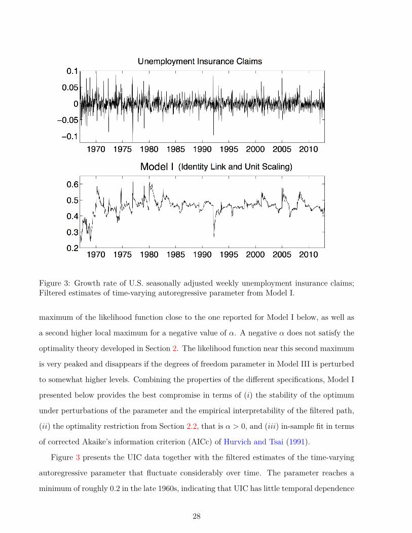
Figure 3: Growth rate of U.S. seasonally adjusted weekly unemployment insurance claims;Filtered estimates of time-varying autoregressive parameter from Model I.

maximum of the likelihood function close to the one reported for Model I below, as well as

a second higher local maximum for a negative value of α. A negative α does not satisfy the

optimality theory developed in Section 2. The likelihood function near this second maximum

is very peaked and disappears if the degrees of freedom parameter in Model III is perturbed

to somewhat higher levels. Combining the properties of the different specifications, Model I

presented below provides the best compromise in terms of (i) the stability of the optimum

under perturbations of the parameter and the empirical interpretability of the filtered path,

(ii) the optimality restriction from Section 2.2, that is α > 0, and (iii) in-sample fit in terms

of corrected Akaike’s information criterion (AICc) of Hurvich and Tsai (1991).

Figure 3 presents the UIC data together with the filtered estimates of the time-varying

autoregressive parameter that fluctuate considerably over time. The parameter reaches a

minimum of roughly 0.2 in the late 1960s, indicating that UIC has little temporal dependence

28

during this time period. In the 1980s, the parameter climbs to about 0.6, indicating that

the UIC may deviate persistently from its unconditional mean over an extended number of

weeks. During the financial crisis of 2008 and its aftermath in 2009, we again see a rise in

the level of persistence of claims, followed by a steady decline until the end of the sample.

5.2 Forecasting comparison for three U.S. economic time series

We consider the one-step ahead forecasting performance of Model I and three benchmark

models. We consider the weekly unemployment insurance claims series from Section 5.1

and two additional series: the U.S. monthly industrial production index from 1947 to 2013,

and the U.S. quarterly money velocity M2 from 1919 to 2013. All three time series are in

log-differences such that we focus on forecasting growth rates. The three series have three

different seasonal frequencies: weekly, monthly and quarterly. The parameter estimates are

obtained from the in-sample analysis.

Table 2 compares the forecast precision of Model I with the forecast precision of the TAR,

STAR and linear AR(p) models for all three series. The order of the AR model p is chosen

by the general-to-specific methodology that selects the lag length based on the minimum

AICc; the optimal order is denoted by p∗. We find that for all three macroeconomic time

series Model I, the TAR, and the STAR model outperform the linear AR model in terms of

root mean squared forecast error by a wide margin. Also, for all three time series, the score

driven Model I has the lowest root mean squared forecast error out of the models considered.

These results are consistent with the likelihood-based results: Model I also outperforms the

TAR, STAR, and AR(p∗) models in terms of the log-likelihood value and AICc.

We conclude that the score driven Model I produces relatively accurate out-of-sample

forecasts for the three U.S. macroeconomic time series. The reported F-RMSEs of Model I

are considerably lower than those of the AR(p∗) models. The nonlinear adaptation to the

serial dependence parameter in Model I is therefore potentially an important feature for the

forecasting of such key economic time series.

29

Table 2: Out-of-sample forecast comparisons for three U.S. macroeconomic time series

The values for the maximized log-likelihood (LogLik), Akaike’s information criterion with finitesample correction (AICc) and root mean squared errors for one-step-ahead forecasts (F-RMSE)of the logarithmic growth rates of U.S. seasonally adjusted time series for weekly unemploymentinsurance claims, monthly industrial production index (2007=100), quarterly money velocityM2; source: Federal Reserve Bank of St. Louis.

Model I TAR STAR AR(p∗)

Weekly Unemployment Insurance Claims, p∗ = 2F-RMSE 0.7502 0.7522 0.7521 0.8484LogLik 6743.96 6736.22 6736.86 6438.89AICc -13477.90 -13462.41 -13463.70 -12869.76

Monthly Industrial Production, p∗ = 3F-RMSE 0.560 0.564 0.563 0.880Log Lik 3025.94 3020.07 3020.50 3020.84AICc -6041.83 -6030.09 -6030.95 -6031.62

Quarterly Money Velocity M2, p∗ = 3F-RMSE 0.1492 0.1514 0.1514 0.2079Log Lik 646.54 643.29 643.30 643.53AICc -1282.79 -1276.31 -1276.32 -1276.78

6 Conclusions

We have shown that updating the parameters in an autoregressive model by the score of

the predictive likelihood results in local improvements of the expected Kullback-Leibler di-

vergence, and thus in nonlinear autoregressive models with information theoretic optimality

properties. The reduced form of the resulting model can be written as a nonlinear ARMA

model that can be compared to alternative nonlinear autoregressive models such as the

threshold and smooth transition autoregressive models. Estimation of the static parameters

in the new model is straightforward, and the maximum likelhood estimator can be shown

to be consistent and asymptotically normal. In our empirical illustration for U.S. unem-

ployment insurance claims, and for two other key U.S. macroeconomic time series, our most

basic nonlinear dynamic model outperforms well-known alternatives such as the threshold

and smooth transition autoregressive models.

30

ReferencesAnderson, P. M. and B. D. Meyer (1997). Unemployment insurance takeup rates and the after-tax value of

benefits. The Quarterly Journal of Economics 112 (3), 913–37.

Anderson, P. M. and B. D. Meyer (2000). The effects of the unemployment insurance payroll tax on wages,employment, claims and denials. Journal of Public Economics 78 (1-2), 81–106.

Ashenfelter, O., D. Ashmore, and O. Deschenes (2005). Do unemployment insurance recipients actively seekwork? evidence from randomized trials in four us states. Journal of Econometrics 125, 53–75.

Blasques, F., S. J. Koopman, and A. Lucas (2014). Maximum likelihood estimation for generalized autore-gressive score models. Discussion Paper, Tinbergen Institute (14-029/III).

Blasques, F., S. J. Koopman, and A. Lucas (2015). Information theoretic optimality of observation driventime series models with continuous responses. Biometrika 102 (2), 325–343.

Bougerol, P. (1993). Kalman filtering with random coefficients and contractions. SIAM Journal on Controland Optimization 31 (4), 942–959.

Chan, K. S. and H. Tong (1986). On Estimating Thresholds in Autoregressive Models. Journal of TimeSeries Analysis 7 (3), 179–190.

Clark, T. E. and M. W. McCracken (2010). Averaging forecasts from VARs with uncertain instabilities.Journal of Applied Econometrics 25, 5–29.

Cox, D. R. (1981). Statistical analysis of time series: some recent developments. Scandinavian Journal ofStatistics 8, 93–115.

Creal, D., S. J. Koopman, and A. Lucas (2011). A dynamic multivariate heavy-tailed model for time-varyingvolatilities and correlations. Journal of Business and Economic Statistics 29 (4), 552–563.

Creal, D., S. J. Koopman, and A. Lucas (2013). Generalized autoregressive score models with applications.Journal of Applied Econometrics 28 (5), 777–795.

Creal, D., S. J. Koopman, A. Lucas, and M. Zamojski (2018). Generalized autoregressive method of moments.Tinbergen Institute Discussion Paper 15-138/III.

Davidson, J. (1994). Stochastic Limit Theory. Advanced Texts in Econometrics. Oxford University Press.

Doan, T., R. B. Litterman, and C. A. Sims (1984). Forecasting and conditional projection using realisticprior distributions. Econometric Reviews 3, 1–144.

Domowitz, I. and H. White (1982, October). Misspecified models with dependent observations. Journal ofEconometrics 20 (1), 35–58.

Freedman, D. and P. Diaconis (1982). On inconsistent m-estimators. Annals of Statistics Vol. 10 (2), pp.454–461.

Gallant, R. and H. White (1988). A Unified Theory of Estimation and Inference for Nonlinear DynamicModels. Cambridge University Press.

31

Gavin, W. T. and K. L. Kliesen (2002). Unemployment insurance claims and economic activity. FederalReserve Bank of St. Louis Review (May), 15–28.

Hansen, B. E. (1991). GARCH(1,1) processes are near epoch dependent. Economic Letters 36, 181–186.

Harvey, A. C. (2013). Dynamic Models for Volatility and Heavy Tails. Cambridge University Press.

Harvey, A. C. and A. Luati (2014). Filtering with heavy tails. Journal of the American Statistical Associa-tion (109), 1112–1122.

Hopenhayn, H. A. and J. P. Nicolini (1997). Optimal unemployment insurance. Journal of Political Econ-omy 105 (2), 412–38.

Hurvich, C. M. and C. Tsai (1991). Bias of the corrected AIC criterion for underfitted regression and timeseries models. Biometrika 78 (3), 499–509.

Kabaila, P. (1983). On the asymptotic efficiency of estimators of the parameters of an arma process. Journalof Time Series Analysis 4 (37-47).

Kadiyala, K. R. and S. Karlsson (1993). Forecasting with generalized Bayesian vector autoregressions.Journal of Forecasting 12, 365–378.

Maasoumi, E. (1990). How to live with misspecification if you must. Journal of Econometrics 44 (1), 67 –86.

McMurrer, D. and A. Chasanov (1995). Trends in unemployment insurance benefits. Monthly Labor Re-view 118 (9), 30–39.

Meyer, B. D. (1995). Natural and quasi-experiments in economics. Journal of Business & Economic Statis-tics 13 (2), 151–61.

Petruccelli, J. (1992). On the approximation of time series by threshold autoregressive models. Sankhya,Series B 54, 54–61.

Pötscher, B. M. and I. R. Prucha (1997). Dynamic Nonlinear Econometric Models: Asymptotic Theory.Springer-Verlag.

Rao, R. R. (1962). Relations between Weak and Uniform Convergence of Measures with Applications. TheAnnals of Mathematical Statistics 33 (2), 659–680.

Straumann, D. and T. Mikosch (2006). Quasi-maximum-likelihood estimation in conditionally heteroeskedas-tic time series: A stochastic recurrence equations approach. The Annals of Statistics 34 (5), 2449–2495.

Teräsvirta, T. (1994). Specification, estimation, and evaluation of smooth transition autoregressive models.Journal of the American Statistical Association 89, 208–218.

Teräsvirta, T., D. Tjostheim, and C. W. J. Granger (2010). Modelling Nonlinear Economic Time Series.Oxford University Press.

Tong, H. (1983). Threshold Models in Non-linear Time Series Analysis. New York: Springer-Verlag.

32

Tong, H. and K. S. Lim (1980). On the effects of non-normality on the distribution of the sample product-moment correlation coefficient. Journal of the Royal Statistical Society, Series B 42 (3), 245–292.

Ullah, A. (1996). Entropy, divergence and distance measures with econometric applications. Journal ofStatistical Planning and Inference 69, 137–162.

Ullah, A. (2002). Uses of entropy and divergence measures for evaluating econometric approximations andinference. Journal of Econometrics 107 (1-2), 313–326.

White, H. (1980, February). Using least squares to approximate unknown regression functions. InternationalEconomic Review 21 (1), 149–70.

White, H. (1981). Consequences and detection of misspecified nonlinear regression models. Journal of theAmerican Statistical Association 76 (374), 419–433.

White, H. (1982, January). Maximum likelihood estimation of misspecified models. Econometrica 50 (1),1–25.

White, H. (1994). Estimation, Inference and Specification Analysis. Cambridge Books. Cambridge UniversityPress.

33

Supplementary Material to:

Nonlinear Autoregressive Models withOptimality Properties1

Francisco Blasques(a), Siem Jan Koopman(a,b), André Lucas(a)

(a) Vrije Universiteit Amsterdam and Tinbergen Institute

(b) CREATES, Aarhus University

A Supplementary Material: Proofs

Proof of Lemma 1. The arguments closely follows those in Blasques et al. (2015) and Creal et al.

(2018), but allowing the scaling function, the score and all conditional densities to depend on yt−1.

In this sense, the results are also slightly different as they establish optimality conditional on yt−1.

We choose score updates with ω = 0, β = 1, and α small, which are termed Newton updates in

Blasques et al. (2015). Note that

Et−1

∫p(y|yt−1) ∂ log p(y|ft, yt−1;θ)

∂f(ft+1 − ft)dy

= Et−1

∫p(y|yt−1) ∇(ft, y, yt−1;θ) (ft+1 − ft) dy

= Et−1

∫p(y|yt−1) ∇(ft, y, yt−1;θ)dy (ft+1 − ft)

=∫p(y|yt−1) ∇(ft, y, yt−1;θ)dy Et−1[ft+1 − ft]

= Et−1[∇(ft, yt, yt−1;θ)] Et−1[ft+1 − ft]

= αS(ft, yt−1;θ) Et−1[∇(ft, yt, yt−1;θ)]2. (A.1)

1Blasques and Lucas thank the Dutch National Science Foundation (NWO; grant VICI453-09-005) forfinancial support. Koopman acknowledges support from CREATES, Aarhus University, Denmark, underthe Danish National Research Foundation grant DNRF78. We thank Howell Tong and Timo Teräsvirta forhelpful comments and suggestions.

34

Using (A.1), we obtain

Et−1

∫p(y|yt−1) log p(y|ft, yt−1;θ)

p(y|ft+1, yt−1;θ)dy (A.2)

= −Et−1

∫p(y|yt−1) ∂ log p(y|ft, yt−1;θ)

∂f(ft+1 − ft)dy

− 12Et−1

∫p(y|yt−1)

∂2 log p(y|f∗t+1, yt−1;θ)∂f2 (ft+1 − ft)2dy

= −αS(ft, yt−1;θ) Et−1[∇(ft, yt, yt−1;θ)]2

− 12Et−1

∫p(y|yt−1)

∂2 log p(y|f∗t+1, yt−1;θ)∂f2 (ft+1 − ft)2dy

= −αS(ft, yt−1;θ) Et−1[∇(ft, yt, yt−1;θ)]2

− 12α

2 S(ft, yt−1;θ)2 Et−1

[(∫p(y|yt−1)

∂2 log p(y|f∗t+1, yt−1;θ)∂f2 dy

)∇(ft, yt, yt−1;θ)2

]

= −αS(ft, yt−1;θ) Et−1[∇(ft, yt, yt−1;θ)]2

− 12α

2 S(ft, yt−1;θ)2 Et−1[It−1(f∗t+1, yt−1) ∇(ft, yt, yt−1;θ)2

], (A.3)

where It−1(f, yt−1) is the conditional Fisher information matrix evaluated at f , i.e.,

It−1(f, yt−1) = Et−1

[∂2 log p(y|f, yt−1;θ)

∂f2

],

and where f∗t+1 is a point between ft+1 and ft.

Due to the misspecification of the filtering density pt for pt and the positivity of α and the

scaling function S(ft, yt−1;θ), the first term in (A.3) is negative. Furthermore, due to the uniform

bounded of It−1(f, yt−1) in f and the existence of the second moment of ∇(ft, yt, yt−1;θ) for every

ft, the second term in (A.3) is negligible compared to the first term for sufficiently small values of

α, i.e., for sufficiently small steps. As a result, we obtain a conditionally expected decrease in the

Kullback-Leibler divergence for small α.

Proof of Lemma 2. The ‘if’ part of the statement follows directly from Lemma 1.

To prove the ‘only if’ part, let ft+1 − ft = φ(ft, yt, yt−1;θ) − ft =: ∆φ(ft, yt, yt−1;θ). Assume

that the update ft+1 = φ(ft, yt, yt−1;θ) is not score-equivalent. Then, by Assumptions 1 and 2, we

can find two open sets Y1 ⊂ R and Y2 ⊂ R for yt for which the following properties hold:

1. ∇(ft, yt, yt−1;θ) > 0∀yt ∈ Y1 and ∇(ft, yt, yt−1;θ) < 0∀yt ∈ Y1;

2. ∇(ft, y∗1, yt−1;θ) = a1 · ∆φ(ft, y∗1, yt−1;θ) for some y∗1 ∈∫

(Y1), and ∇(ft, y∗2, yt−1;θ) = a1 ·

∆φ(ft, y∗2, yt−1;θ) for some y∗2 ∈∫

(Y2), and a1 6= a2 6= 0.

35

Now consider sufficiently small neighborhoods Y ∗1 and Y ∗2 such that y∗1 ∈ Y ∗1 ⊂ Y1 and y∗2 ∈ Y ∗2 ⊂ Y2.

Also select a true density pt that puts all its probability mass on the regions Y ∗1 and Y ∗2 in such a

way that Et−1[∇1] = 0. Given a1 6= a2, we have for this particular pt that Et−1[∆φ(ft, y∗1, yt−1;θ)]

is either strictly positive or strictly negative. Assume Et−1[∆φ(ft, y∗1, yt−1;θ)] > 0. The converse

argument holds for Et−1[∆φ(ft, y∗1, yt−1;θ)] < 0. Then we can construct a new density p∗t that

assigns slightly more weight to Y ∗2 and slightly less to Y ∗1 , thus resulting in E∗t−1[∇1] < 0 and

Et−1[∆φ(ft, y∗1, yt−1;θ)] > 0, where E∗t−1[ · ] denotes the expectation with respect to p∗t . Then for

this p∗t and following the arguments in the proof of Lemma 1, the steps induced by φ result in a

deterioration of the EKL divergence, such that φ does not induce EKL optimality. We conclude

that an update that is not score equivalent is not EKL optimal.

Proof of Theorem 1: The proof follows directly from Blasques et al. (2014, Propositions TA.1

and TA.2). The only difference is that the innovations of the updating equation are now a vector

given by (yt−1, yt−2). Otherwise the proof is still the same.

In particular, we obtain the uniform e.a.s. convergence of the filter

supθ∈Θ|ft(y1:t−1,θ, f1)− ft(yt−1,θ)| e.a.s.→ 0, (A.4)

by considering the sequence {ft(y1:t−1, ·, fΘ1 )}t∈N with elements ft(y1:t−1, ·, fΘ

1 ) taking values in

the separable Banach space FΘ ⊆ (C(Θ, F), ‖ · ‖Θ) with initialization fΘ1 in C(Θ, F) at t = 1,

fΘ1 (θ) = f1 ∀ θ ∈ Θ, and

ft(y1:t, ·, fΘ1 ) = φt

(ft(y1:t−1, ·, fΘ

1 ))∀ t ∈ N,

where {φt}t∈Z is a sequence of stochastic recurrence equations φt : Ξ× C(Θ, F)→ C(Θ, F) ∀ t as

in Straumann and Mikosch (2006, Proposition 3.12).

Blasques et al. (2014, Propositions TA.1 and TA.2) show that the uniqueness and e.a.s. con-

vergence can be obtained through the application of Straumann and Mikosch (2006, Theorem 2.8),

and that the bounded moments can be ensured by unfolding the process backwards to obtain

supt‖ft(·, fΘ

1 )− fΘ‖Θnf≤

t−2∑j=0

(c)j((c+ 1)f + ¯φ) + ct−1 supt‖fΘ

1 − fΘ‖Θnf

≤ (c+ 1)f + ¯φ1− c + ‖fΘ

1 − fΘ‖Θnf<∞.

36

Proof of Theorem 2: The result follows by noting that the condition imposed on s ensures the

contraction condition in Theorem 6.10 of Pötscher and Prucha (1997) for the parameter recursion.

Furthermore, the moment bound in part (c) of their theorem holds because {yt} is SE and has two

bounded moments. The moment bounds on the initialization in their theorem also hold trivially

since f1 is constant.

Proof of Theorem 3: This proof is immediate given Blasques et al. (2014, Theorem 4.6), after

slightly augmenting the notation to include yt−1 in the appropriate conditioning and argument sets.

In particular, in Blasques et al. (2014, Theorem 4.6), the existence and measurability of θTis obtained through an application of White (1994, Theorem 2.11) or Gallant and White (1988,

Lemma 2.1, Theorem 2.2), and the consistency of the MLE, θT (f1) a.s.→ θ0, is obtained by White

(1994, Theorem 3.4) or Gallant and White (1988, Theorem 3.3), from the uniform convergence of

the log likelihood function

supθ∈Θ|LT (θ, f1)− `∞(θ)| a.s.→ 0 ∀ f1 ∈ F as T →∞, (A.5)

and the identifiable uniqueness of the maximizer θ0 ∈ Θ introduced in White (1994),

supθ:‖θ−θ0‖>ε

`∞(θ) < `∞(θ0) ∀ ε > 0. (A.6)

Additionally, Blasques et al. (2014, Theorem 4.6) establish the uniform convergence of the

criterion by showing invertibility of the filtering process and by applying the ergodic theorem for

separable Banach spaces in Rao (1962) to the limit likelihood sequence {LT (·)} with elements

taking values in C(Θ,R).

The identifiable uniqueness is ensured by the uniqueness of θ0 as the maximizer of the likelihood,

the compactness of Θ, and the continuity of the limit likelihood function E`t(θ) in θ ∈ Θ, which is

also shown in Blasques et al. (2014, Theorem 4.6).

Proof of Theorem 4: The proof can be found in Blasques et al. (2014, Theorem 4.14), with some

change in notation to include yt−1 in the appropriate conditioning and argument sets. In particular,

we can obtain the asymptotic normality using White (1994, Theorem 6.2), which involves: (i) the

consistency of θTa.s.→ θ0 ∈ int(Θ); (ii) the a.s. twice continuous differentiability of LT (θ, f1) in

θ ∈ Θ; (iii) the asymptotic normality of the score

√TL′T

(θ0, f

(0:1)1 ) d→ N(0, J(θ0)

)as T →∞, where J(θ0) = E

(`′t(θ0))2; (A.7)

where f (0:1)1 denotes the partial derivative process; (iv) the uniform convergence of the likelihood’s

37

second derivative,

supθ∈Θ

∥∥L′′T (θ, f (0:2)1 )− `′′∞(θ)

∥∥R16

a.s.→ 0 as T →∞ ; (A.8)

and finally, (v) the non-singularity of the limit `′′∞(θ) = E`′′t (θ) = I(θ).

Blasques et al. (2014, Theorem 4.14) obtain the asymptotic normality of the score through the

invertibility of the filter and its derivative processes, and by application of the central limit theorem

(CLT) for NED sequences of Pötscher and Prucha (1997) to obtain

√TL′T

(θ0) d→ N(0, I(θ0)

)as T →∞. (A.9)

The uniform convergence of the Hessian is obtained through the invertibility of the filter and

its derivative processes, and by application of the ergodic theorem for separable Banach spaces in

Rao (1962) to the limit Hessian (see also Straumann and Mikosch (2006, Theorem 2.7)).

B Small Sample Properties

We analyze the filtering properties of our nonlinear ARMA modeling framework in a simulation

setting. In particular, our Monte Carlo set-up focuses on the finite-sample performance of the filter

when the data generating process for {yt} is given by

yt = ftyt−1 + ut, ut ∼ N(0, λ),

with {ft} following a sinusoid pattern

ft = 0.5 + 0.5 sin(t/150).

Figure B.1 is based on 1000 Monte Carlo simulations. For each simulation, we estimate the

path of the time varying parameter. We do so for a sample size of T = 500 and T = 1500. The

figure displays the true path of {ft} as well as the paths filtered by Models I and II. The cloud of

dots are filtered points {ft}. The dashed lines are pointwise bounds containing 95% of the mass of

the filter over the 1000 Monte Carlo repetitions.

The results in Figure B.1 illustrate how different specifications of the autoregressive model for

{yt} can lead to score filters for {ft} with different properties. While Figure B.1 shows that both

models perform well, it also reveals that Model II (with the logistic link function) outperforms

Model I (with the unit link function). In particular, Model I tends to do worse during periods of

low dependence.

38

Figure B.1: The figure presents 1000 draws in a Monte Carlo performance for Model I (left)and Model II (right) for sample sizes T = 500 (top) and T = 1500 (bottom). True ft in red,fitted ft as gray dots, with mean and 95% confidence band in black.

39