ORIGINAL ARTICLE

Niels Wessel Æ Hagen Malberg Æ Robert Bauernschmitt

Alexander Schirdewan Æ Jurgen Kurths

Nonlinear additive autoregressive model-based analysis of short-termheart rate variability

Received: 8 August 2005 / Accepted: 27 February 2006 / Published online: 29 March 2006� International Federation for Medical and Biological Engineering 2006

Abstract In this contribution we test the hypothesis thatnonlinear additive autoregressive model-based dataanalysis improves the diagnostic ability based on short-term heart rate variability. For this purpose, a nonlinearregression approach, namely, the maximal correlationmethod is applied to the data of 37 patients with dilatedcardiomyopathy as well as of 37 age- and sex-matchedhealthy subjects. We find that this approach is a pow-erful tool in discriminating both groups and promisingfor further model-based analyses.

Keywords Nonlinear regression Æ Heart ratevariability Æ Modeling Æ Time series analysis

1 Introduction

Most cardiovascular diseases are characterized by a slowprogression leading to possibly abrupt qualitative chan-ges [24, 49]. This pathogenesis is a dynamic process andthe associated cardiovascular parameters, such as heartrate variability (HRV), exhibit complex dynamics [3, 7,25, 30]. Accordingly, the central requirement of nonlineardynamics aims exactly at such physiological phenomena.First applications of nonlinear dynamics tools in medical

diagnostics met with success in the last 10 years [11, 20].So far, however, either only data were analyzed [8, 13, 19,28, 31, 42, 47, 48] or models developed [12, 14, 32, 45, 46].The purpose of this paper therefore is, to take a qualita-tively new step for HRV data: the combination of dataanalysis and modeling. Model-based nonlinear-dynamicdata analysis of non-invasivelymeasured biosignals couldlead to an improved diagnostic ability and to a betterunderstanding of the cardiovascular regulation. Appli-cations of the research results are manifold: Monitoring-,diagnosis-, course- and mortality prognoses as well as theearly detection of heart diseases. As regards clinicalapplications, there is an extraordinary demand for newcomputer-controlled diagnostic methods to obtain amore exact and differentiated picture of the possiblydamaged heart.

The analysis of HRV has become a powerful tool forthe assessment of autonomic control. HRV measure-ments have proven to be independent predictors ofsudden cardiac death after acute myocardial infarction,chronic heart failure or dilated cardiomyopathy [17, 21,27, 33, 34, 38]. Moreover, it has been shown that short-term HRV analysis already has an independent prog-nostic value in risk stratification apart from that ofclinical and functional variables [23]. However, theunderlying regulatory mechanisms are still poorlyunderstood. Short-term heart rate (HR) regulation isaccomplished mainly by neural sympathetic- and para-sympathetic-mediated cardiac baroreflexes and periph-eral vessel resistance, whereas long-term regulation isachieved by hormonal pathways as well as other systemslike the renin-angiotensin-system [4]. To gain more in-sight into cardiovascular regulation, in this paper anonlinear additive autoregressive (NAAR) model isestimated nonparametrically. The nonlinear regressionmethod we are using was introduced by Breiman andFriedman [6] in 1985 and already successfully applied toNAAR modeling of riverflow data in 1993 [9].

The paper is organized as follows. In Sect. 2 weshortly describe the data, HRV parameters as well asthe nonlinear regression approach used. In Sect. 3 the

N. Wessel (&) Æ J. KurthsInstitute of Physics, University of Potsdam,Am Neuen Palais 10, 14415 Potsdam, GermanyE-mail: wessel@agnld.uni-potsdam.de

R. Bauernschmitt Æ N. WesselClinic for Cardiovascular Surgery,German Heart Center Munich, Lazarettstr. 36,80636 Munich, Germany

A. Schirdewan Æ N. WesselMedical Faculty of the Charite, Franz Volhard Clinic, HeliosKlinikum-Berlin, Wiltbergstr. 50, 13125 Berlin, Germany

H. MalbergInstitute for Applied Computer Science/Automation (AIA),University of Karlsruhe (TH), Kaiserstraße 12, 76128Karlsruhe, Germany

Med Biol Eng Comput (2006) 44: 321–330DOI 10.1007/s11517-006-0038-0

results of standard HRV analysis, nonlinear modelingand simulating shall be presented. Finally, in Sect. 4 theresults shall be discussed.

2 Methods

This study is aimed at investigating short-term HRrecordings of 37 patients with dilated cardiomyopathy(DCM, age: 50.2±9.1 years) in comparison to 37 heal-thy subjects (52.1±6.7 years). The diagnosis of DCMwas established in according to the recommendations formedical testing of patients with cardiomyopathy. TheDCM patients had a left ventricular ejection fraction of22.3±5.7%, a New York Heart Association class ofII–III and were getting the present standard therapy[ACE-inhibitor (31), beta-blocker (16), diuretics (27)].All patients were in sinus rhythm and had no concom-itant diseases. To minimize the probability for cardiacdiseases in the healthy volunteers group we recruitedthem from an occupational health center. They hadnormal findings in echocardiography, bicycle ergometry,and Holter ECG for many years. No control subject hada history of cardiac diseases or symptoms. Patientcharacteristics are summarized in Table 1. All mea-surements were performed under comparable ambientconditions (before noon, after having a small breakfast,same place, temperature) with a standard ambulatoryECG (100 Hz) for 30 min under supine position. Theconsumption of alcohol and tobacco was forbidden 24 hbefore the measurement.

Ventricular premature beats as well as artifacts werefiltered out using a special adaptive filtering proceduredescribed in [39]. Figure 1a and b give examples of thesedata sets. To demonstrate later on where the nonlinearregression approach is adequate, a time series of a patientwith atrial fibrillation from another study is given inFig. 1c.

2.1 Heart rate variability analysis

Heart rate variability is calculated in the time andfrequency domain regarding the Task Force HRV [17]and by methods of nonlinear dynamics. AnalyzingHRV, the following standard parameters are calcu-lated from the time series: MeanNN (mean value ofnormal beat-to-beat intervals): Inversely related tomean HR. sdNN (SD of intervals between two normalR-peaks): Gives an impression of the overall circula-tory variability. sdaNN (the SD of successive 5 min’NN-interval mean values): quantifies long-range vari-abilities. rmssd (root mean square of successiveRR-intervals) and pNN50 (percentage of RR-interval-differences greater than 50 ms): quantifying short-range variabilities. Shannon (the Shannon entropyof the histogram): quantification of RR-interval dis-tribution. Apart from the time-domain parametersmentioned above, the HRV analysis focused on high-frequency (HF), low-frequency (LF) and very-low-frequency (VLF) components expressed by thenormalized values LF/P, HF/P, VLP/P, and the ratioLF/HF (where P is the total power). The number ofventricular ectopic beats is automatically counted anddenoted by noNNtime (cumulative time of not normalbeat-to-beat intervals). Finally, HRV is analyzed bymethods of nonlinear dynamics, especially symbolicdynamics [22, 36, 40, 41]: In this analysis the timeseries are transformed into symbol sequences withsymbols from a given alphabet. Some details are lostin this process; however, the advantage is that thecoarse dynamic behavior can be analyzed. The usedparameter ‘Polvar20’ (Probability of low variability,20 ms difference) characterizes short phases of lowvariability from successive symbols of a simplealphabet, consisting of only the symbols 0 and 1,where 0 stands for a small difference of less than20 ms between two successive beat-to-beat intervals,and where 1 represent cases when the differencebetween two successive beat-to-beat intervals exceedsthis limit, specifically given the time series x1,x2,...,xNone obtains the symbol series sn

sn ¼1 : jxn � xn�1j � 20ms0 : jxn � xn�1j\20ms

�ð1Þ

Words consisting of the unique symbols all 0 or all 1 arecounted. To obtain a statistically robust estimate of theword distribution, we restrict ourselves to the 64 wordsdefined by six consecutive symbols. ‘Polvar20’ representsthe probability of the word 000000 occurring and thusdetects even intermittently decreased HRV.

2.2 Model-based data analysis

We generally assume that there are HR time series Xi,i=1,...,n (series of beat-to-beat-intervals as in Fig. 1). Inthis paper the following class of NAAR-models shall beconsidered

Table 1 Patient characteristics

Group Control, n=37 DCM, n=37

Age (years) 50.2±9.1 52.1±6.7SexMale 26 27Female 11 10SBP (mmHg) 119.0± 18.6 110.6±12.4*DBP (mmHg) 73.2± 7.8 70.5±9.9HR (bpm) 69.5± 9.4 75.4±7.6*EchoLVEF (%) – 22.3±5.7LVDD (mm) – 67.8±8.6PharmacotherapyACEI – 31b-blocker – 16Diuretic – 27

SBP systolic blood pressure, DBP diastolic blood pressure, HRheart rate, LVEF left ventricular ejection fraction, LVDD leftventricular diastolic diameter, ACEI angiotensin-converting en-zyme inhibitor*P<0.05 versus control group

322

hðXjÞ ¼Xk

i¼1/iðXj�iÞ; j ¼ k þ 1; . . . ; n: ð2Þ

where k denotes the history length. The alternatingconditional expectations (ACE) algorithm [6] describedbelow is applied as a nonparametric approach to esti-mate the possibly nonlinear transformations /i and h inEq. 2. The easiest model of this class is the linearautoregressive model

Xj ¼Xk

i¼1ai � Xj�i; j ¼ k þ 1; . . . ; n: ð3Þ

The concept of maximal correlation is a very powerfulcriterion to measure the dependence in particular ofnonlinear related variables [29]. The main idea of thisapproach is to measure the maximized correlation ofproperly transformed variables.

Given a real variable Xj and a ni-dimensional vectorX ¼ ðX1; . . . ;XniÞ in the additive model 2. Then, themaximal correlation is defined by

WðXj;X Þ :¼jqðh�ðXjÞ;/�ðX ÞÞj¼max

h;/jqðhðXjÞ;/ðX ÞÞj ð4Þ

where q denotes the correlation coefficient. The functionsh* and /*, which fulfil the maximal condition (4), arecalled optimal transformation and represent an estima-tion of the model 2. To estimate them nonparametrically,we use the ACE-algorithm [6]. Afterwards, to enable aclassification of these transformations, a polynomial fit-ting was performed to parametrize the model functions.For more details to the ACE-algorithm see the Appendix.

The maximal correlation and optimal transformationapproach were applied recently to nonlinear dynamic

systems to identify delay in lasers [35] and partial dif-ferential equations in fluid dynamics [37]. The ACEalgorithm turned out to be a very efficient tool fornonlinear data analysis [16, 35, 39, 43, 44].

3 Results

3.1 Heart rate variability

The DCM group was characterized by a increased HR(consequently, by a lower meanNN) and a decreasedHRV as reflected by the parameters sdNN and sdaNN5(see Table 2). Interestingly, both groups hardly differedin the respiration-induced very short variability range(rmssd). Both, the increased HR and the decreased HRVlead to significantly different Shannon entropies of theRR-interval distribution of the groups. In frequencyanalysis, an increased VLF band is observed for theDCM group, whereas the LF band is decreased. Again,no significant differences result in the respiration-induced and vagally mediated HF band. The significantdifferences of LF/HF between both groups is due to thelower LF band in the DCM group exclusively. Surpris-ingly, parameters from symbolic dynamics did not showany significant difference between both groups (only as atrend ‘Polvar20’: p=0.057). Finally, the DCM patientsshow a higher level of ventricular ectopy (NoNNtime).

3.2 Model-based data analysis

For simplicity reasons, we started with a linear autore-gressive model given in Eq. 3. For different model ordersup to 10, linear autoregressive modeling was performedand the model coefficients themselves were considered to

0 200 400 600 800 1000 1200 1400 1600 1800200

400

600

800

1000

1200(a)

BB

I in

[ms]

0 200 400 600 800 1000 1200 1400 1600 1800200

400

600

800

1000

1200(b)

BB

I in

[ms]

0 200 400 600 800 1000 1200 1400 1600 1800200

400

600

800

1000

1200(c)

n

BB

I in

[ms]

Fig. 1 Thirty minutestachograms from a healthyvolunteer (a), a patient withdilated cardiomyopathy (b) anda patient with atrial fibrillation(c) [beat-to-beat-interval (BBI)]

323

be parameters for discrimination between DCM andcontrols. The model coefficients however, were signifi-cant only up to the order 2 (cf. Table 3). The residualvariance g was significantly lower in the DCM group,certainly caused by the lower HRV in this group. Theabsolute values of the coefficients a1 and a2 were higherfor the controls, indicating a higher dependence from thetwo predecessors for healthy subjects.

Based on the findings from linear autoregressivemodeling, a NAAR-model of order 2 given in Eq. 5 wasinvestigated.

Xj ¼ /1ðXj�1Þ þ /2ðXj�2Þ; j ¼ 3; . . . ; n: ð5Þ

The left hand side of Eq. 5 is the identity and we areinterested in estimating the functional dependence of Xj

on its two predecessors. Figure 2 gives this functionalrelationship that was estimated from the time series gi-ven in Fig. 1. We see a nonlinear functional relation forboth the healthy and the DCM subject in Fig. 2a and b.For the subject with atrial fibrillation in Fig. 2c, how-ever, no real functional relationship could be estimated.In this case, the random influence is too strong, the RR-intervals are nearly uncorrelated. This example showsthat there has to be a minimal relation between the dataat least for applying this nonlinear regression approach.

The concept of maximal correlation and optimaltransformations is a nonparametric approach which al-lows to estimate in particular nonlinear dependenciesbetween two variables. However, in this paper the aimwas to quantify these relations. Therefore, polynomial

fitting of third order was performed. The fitting coeffi-cients themselves were considered to be parameters incardiac diagnostics.

Xj ¼ a1 � X 3j�1 þ a2 � X 2

j�1 þ a3 � Xj�1 þ a4

þ b1 � X 3j�2 þ b2 � X 2

j�2 þ b3 � Xj�2 þ b4 j ¼ 3; . . . ; n:

ð6Þ

Using higher orders for polynomial fitting turned outnot to be useful in this study. Figure 2 gives the fittedpolynomials in addition to the optimal transformation.These fitting parameters did not differ statistically be-tween DCM and control for /1. Table 4 gives the fittingparameters for /1 and /2 and we see that parameter b3has the smallest p-value of all considered parameters inthis study.

To compare these fitting parameters directly withstandard HRV parameters we performed a tenfoldbootstrap approach. We repeatedly analyzed subsam-ples of the data based on discriminant function analyses.Each subsample was a random sample with 70%replacement from the full sample (resampling). We usedten different permutation of the data as training sets andthe best three parameters to separate the groups werechosen. The parameter b3 was automatically selected innine of ten validation runs which demontrates thereliability of our results. The best combination ofparameters to separate controls from DCM were thefitting parameter b3, the normalized very low frequency‘VLP/P’ as well as the number of ventricular prematurebeats, quantified by the preprocessing parameter‘noNNtime’. The averaged classification rates of thistenfold bootstrap validation were 82.1% for the trainingset (optimistic estimation) and 73.2% for the 30% testset (realistic estimation).

Figure 3 visualizes the polynomial fitting of /1 and/2 from Eq. 5 based on group averages. While theoptimal transformations /1 are similar for the DCM andthe control group (except the small difference at largerbeat-to-beat-intervals—leading a4 close to be signifi-cant), the behavior of /2 is totally different in bothgroups. The coefficients b1 and b2, representing thequadratic and the cubic part of the fitting and thereforelower than b3 and b4, both are higher in absolute valuesfor the DCM subjects and lead to a more oscillatingbehavior of this fitting for this group. The coefficient b3,representing the linear part of the fitting, is b3=0.045 forthe control subjects and, hence, higher than b3=�0.61for the DCM group. This means that we have a lineartendency for a slight increase of /2 with increasing beat-to-beat-interval, whereas, the DCM group exhibits aclear decrease. The dominant part for the discriminationof both groups however, is the quadratic term b2 whichis extremely higher in the DCM group. Thus, for theinterpretation of these results all fitting coefficients haveto be considered together.

To investigate the stability of our approach we per-formed Monte-Carlo simulations based on the group

Table 2 Results of heart rate variability (HRV) analysis

Control DCM p

meanNN 903.48±129.90 810.07±106.16 0.0013*sdNN 50.70±19.86 41.04±20.76 0.0099sdaNN5 25.10±12.60 17.34±11.53 0.0008*rmssd 29.84±15.17 24.25±8.95 NSpNN50 0.085±0.109 0.039±0.039 NSShannon 2.21±0.38 1.99±0.40 0.0123LF/HF 2.89±2.15 1.97±1.44 0.0270LF/P 0.24±0.10 0.18±0.09 0.0038*HF/P 0.12±0.07 0.13±0.08 NSVLF/P 0.40±0.12 0.50±0.19 0.0416NoNNtime 17.0±23.3 38.3±38.2 0.0064Polvar20 0.07±0.15 0.11±0.14 NS

Mean value ± SD, two-sided Mann–Whitney U test*Significant after Holm correction [18])

Table 3 Results of linear autoregressive model analysis

Control DCM p

a1 0.96±0.08 0.90±0.08 0.0011*a2 �0.05±0.12 0.02±0.10 0.0068*g 1,766±1159 1,111±539 0.0026*

Mean value ± SD, two-sided Mann–Whitney U test. g representsthe residual variance*Significant after Holm correction

324

averaged polynomials given in Fig. 3. Two examples aregiven in Fig. 4. Initial values X1 and X2 for both simu-lations were 1,000 as one can expect from this figure.Then all simulated values were calculated as follows

Xj ¼ a1 � X 3j�1 þ a2 � X 2

j�1 þ a3 � Xj�1 þ a4

þ b1 � X 3j�2 þ b2 � X 2

j�2 þ b3 � Xj�2

þ b4 þ g j ¼ 3; . . . ; n: ð7Þ

were g is a normally distributed random number withmean zero and SD 15 ms. Interestingly, the differentmean HRs in both groups are achieved already after afew iterations. Due to the strong relationship each HRvalue to its two predecessors, we get a more homoge-neous behavior in the control group, whereas the DCMsimulation is characterized by some drops (e.g. around

sample 1,100). From these simulations again the poly-nomial coefficients were estimated using the approachdescribed. Figure 5 shows these functions which are verysimilar to the polynomials in Fig. 3. There is only asmall horizontal shift of /1 in the DCM and of /2 in thecontrol group, the qualitative behavior is remained.Thus, our method is able to consistently obtain impor-tant information from the time series, which indicates apossible use for surrogate data analysis.

Finally, we investigated whether our developedmodels are useful for the forecasting of HR data. Forthis reason, one-step predictions based on two prede-cessors Xj-1 and Xj-2 and the optimal transformationsestimated from Eq. 5 were performed. Figure 6 gives theresults of these simulations from the tachograms intro-duced in Fig. 1. We see adequate estimations for thecontrol as well as for the DCM series, the time series arevery similar to the ones given in Fig. 1. For the patientwith atrial fibrillation, however, no comparable resultswere obtained. The one-step predictions fail due to thefact that the optimal transformations do not represent areal functional relationship.

4 Discussion

The main purpose of this paper was to test whethermodel-based data analysis improves the results of diag-nostic ability based on short-term HRV. Hence, firstlystandard HRV analysis was performed: The DCM pa-tients are mainly characterized by a increased HR, a

0 500 1000 1500400

600

800

1000

BBI [ms]

Φ1(B

BI)

[ms]

0 500 1000 1500–200

–100

0

100

200

BBI [ms]

Φ2(B

BI)

[ms]

(a)

0 500 1000 1500400

600

800

1000

BBI [ms]

Φ1(B

BI)

[ms]

0 500 1000 1500 –200

–100

0

100

200

BBI [ms]

Φ2(B

BI)

[ms](b)

0 500 1000 1500400

600

800

1000

BBI [ms]

Φ1(B

BI)

[ms]

0 500 1000 1500 –200

–100

0

100

200

BBI [ms]

Φ2(B

BI)

[ms](c)

Fig. 2 Optimal transformationsas well as estimatedpolynomials for the tachograms(a), (b) and (c) from Fig. 1(BBI)

Table 4 Results of NAAR-model-based HRV analysis

Control DCM p

W 0.844±0.082 0.841±0.084 NSa1 �1.3E�06±7.4E�07 �1.3E�06±1.2E�06 NSa2 3.1E�03±1.4E�03 2.8E�03±1.8E�03 NSa3 �1.621±0.749 �1.356±0.701 NSa4 800.7±118.8 745.1±98.2 0.061b1 �5.9E�08±8.8E�07 �7.8E�07±1.2E�06 0.0019*b2 1.9E�05±1.6E�03 1.4E�03±1.9E�03 0.0011*b3 0.045±0.744 �0.606±0.758 0.0006*b4 �4.92±27.59 �13.72±17.69 NS

Mean value ± SD, two-sided Mann–Whitney U test*Significant after Holm correction

325

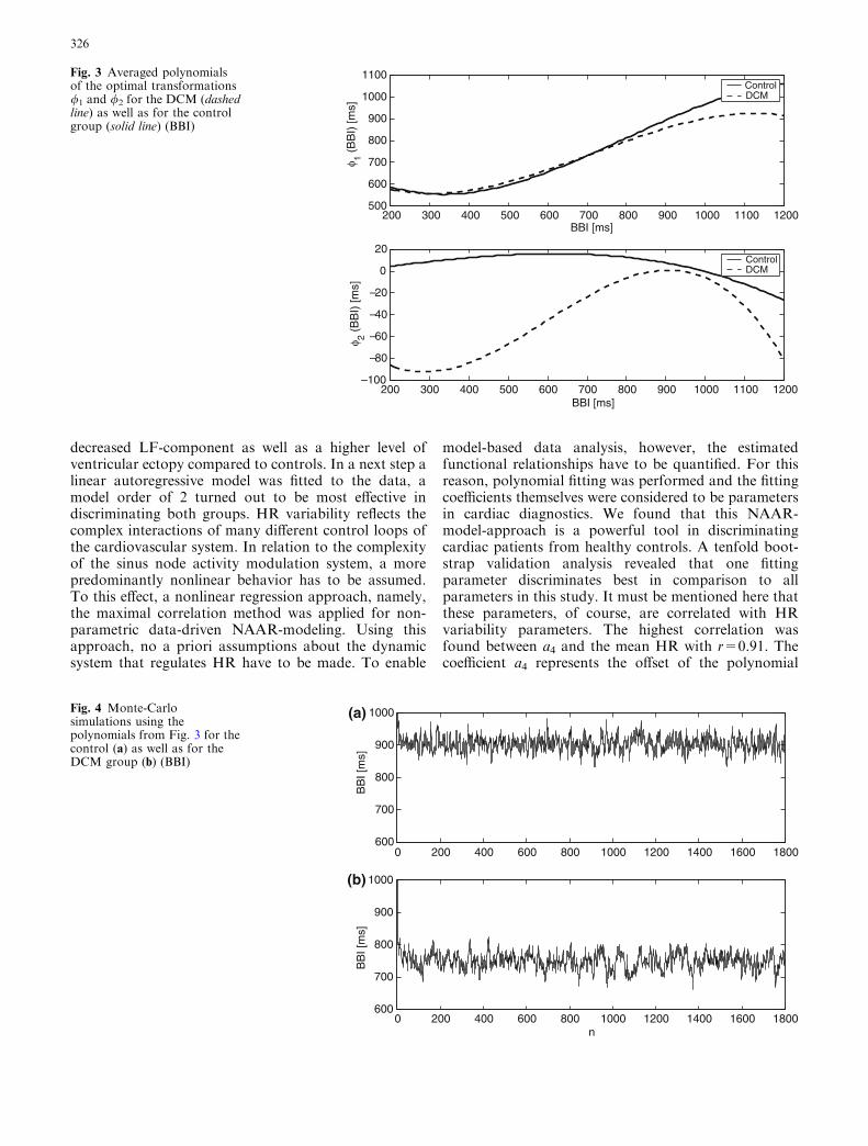
decreased LF-component as well as a higher level ofventricular ectopy compared to controls. In a next step alinear autoregressive model was fitted to the data, amodel order of 2 turned out to be most effective indiscriminating both groups. HR variability reflects thecomplex interactions of many different control loops ofthe cardiovascular system. In relation to the complexityof the sinus node activity modulation system, a morepredominantly nonlinear behavior has to be assumed.To this effect, a nonlinear regression approach, namely,the maximal correlation method was applied for non-parametric data-driven NAAR-modeling. Using thisapproach, no a priori assumptions about the dynamicsystem that regulates HR have to be made. To enable

model-based data analysis, however, the estimatedfunctional relationships have to be quantified. For thisreason, polynomial fitting was performed and the fittingcoefficients themselves were considered to be parametersin cardiac diagnostics. We found that this NAAR-model-approach is a powerful tool in discriminatingcardiac patients from healthy controls. A tenfold boot-strap validation analysis revealed that one fittingparameter discriminates best in comparison to allparameters in this study. It must be mentioned here thatthese parameters, of course, are correlated with HRvariability parameters. The highest correlation wasfound between a4 and the mean HR with r=0.91. Thecoefficient a4 represents the offset of the polynomial

200 300 400 500 600 700 800 900 1000 1100 1200500

600

700

800

900

1000

1100

BBI [ms]

φ 1 (B

BI)

[ms]

ControlDCM

200 300 400 500 600 700 800 900 1000 1100 1200 –100

– 80

– 60

– 40

–20

0

20

BBI [ms]

φ 2 (B

BI)

[ms]

ControlDCM

Fig. 3 Averaged polynomialsof the optimal transformations/1 and /2 for the DCM (dashedline) as well as for the controlgroup (solid line) (BBI)

0 200 400 600 800 1000 1200 1400 1600 1800600

700

800

900

1000(a)

BB

I [m

s]

0 200 400 600 800 1000 1200 1400 1600 1800600

700

800

900

1000

n

(b)

BB

I [m

s]

Fig. 4 Monte-Carlosimulations using thepolynomials from Fig. 3 for thecontrol (a) as well as for theDCM group (b) (BBI)

326

fitting, and thus, the minimum beat-to-beat-interval,which obviously is correlated with the mean heart rate.The most significant coefficient b3, however, did notshow such high correlations with HRV parameters, thehighest was found for LF/P with r=0.50. The highestcorrelation for the coefficients b1 and b2 were r=�0.46(to LF/P) and r=0.41 (to meanNN), respectively. In thisregard, the decrease of low frequency together with theapparently less effective baroreflex regulation in DCMpatients may explain the differences in /2 between bothgroups. For the controls, we got a strong relationshipbetween one beat-to-beat-interval and its pre-predeces-

sor, whereas this clear relation is weakened for the DCMgroup. The Monto-Carlo simulations performed in thisstudy confirmed these findings, the control subjects showa more homogeneous and stable behavior in HRV. Ourresults clearly indicate, that the NAAR-model parame-ters contain important additional information in com-parison to HRV parameters. The simulation studyshowed that one-step predictions based on optimaltransformations gave promising results. For subjectswith atrial fibrillation or ventricular ectopy, however, noreal functional relationship could be estimated. A pre-condition for applying this method are at least minimal

200 300 400 500 600 700 800 900 1000 1100 1200500

600

700

800

900

1000

1100

BBI [ms]

φ 1 (B

BI)

[ms]

ControlDCM

200 300 400 500 600 700 800 900 1000 1100 1200 –100

–80

–60

–40

–20

0

20

40

BBI [ms]

φ 2 (B

BI)

[ms]

ControlDCM

Fig. 5 Polynomials estimatedfrom the Monte-Carlosimulations in Fig. 4 for theDCM (dashed line) as well asfor the control group (solid line)(BBI)

200 400 600 800 1000 1200 1400 1600 1800200400600800

10001200(a)

BB

I [m

s]

200 400 600 800 1000 1200 1400 1600 1800200400600800

10001200(b)

BB

I [m

s]

200 400 600 800 1000 1200 1400 1600 1800200400600800

10001200(c)

n

BB

I [m

s]

TrainingTraining TestFig. 6 One step predictions(solid line) of the tachograms(a), (b) and (c) from Fig. 1 usingthe optimal transformationestimated from the training set(first three quarters of theoriginal data set—dotted line)and the last two values (BBI)

327

correlations in the data and the exlusion of artifacts. Allresults remain to be validated on a larger data base andit will have to be investigated whether more sophisti-cated models, such as polynomial fittings or NARMA-models [1, 2, 5, 10, 15, 26], improve model-based dataanalysis in risk stratification of cardiac patients. Sum-marizing the results of this paper, we find that the ACEalgorithm is a powerful tool to estimate the transfor-mations h and / in the analyzed model and, thus, en-ables the qualitatively new step: the combination of dataanalysis and modeling. Model-based nonlinear-dynamicdata analysis of non-invasively measured biosignals leadto an improved clinical diagnostics in this study. LaRovere et al. [23] showed that short-term HRV analysishas an independent prognostic value in risk stratificationapart from that of clinical and functional variables. Ourintroduced methodology is able to detect changes incardiovascular variability due to cardiac dysfunctionexemplary for DCM patients. It has to be mentionedhere, that this study was an exclusively methodologicalinvestigation and has minor relevance for diagnosingDCM patients. However, improving these modelingtechniques and understanding the underlying mecha-nisms may lead to the detection of cardiac dysfunctionbased on Holter monitoring in the future. Therefore, ourapproach seems to be very promising also for otherbiosignal processing, e.g. blood pressure variability ormultivariate cardiovascular modeling with nonlinearinteractions and feedback loops.

Acknowledgments We would like to thank Henning Voss for pro-viding the Matlab-code and very helpful discussions as well as theDeutsche Forschungsgemeinshaft (DFG BA 1581/4-1, BR 1303/8-1, KU 837/20-1) for supporting the study.

5 Appendix: the ACE algorithm

This appendix provides a short description of the ACEalgorithm of Breiman and Friedman [6], the computerprograms used can be obtained from the authors(http://tocsy.agnld.uni-potsdam.de/). In the followingsection, the same notations as introduced in Sect. II areused.

Generally, the estimation of functions that are opti-mal for correlation is equivalent to the estimation offunctions that are optimal for regression. Therefore, theproblem

WðS; T1; . . . ; TkÞ ¼ maxh;/i

qðhðSÞ;Xk

i¼1/iðTiÞÞ

���������� ð8Þ

may also be expressed as the regression problem

E hðSÞ �Xk

i¼1/iðTiÞ

!224

35!¼min : ð9Þ

Here, the functions h and /j (j=1,...,k) are varied inthe space of Borel measurable functions, and the con-straints onto these functions are that they have vanish-ing expectation and finite variances to exclude trivialsolutions.

For the one-dimensional case (k=1), the ACE algo-rithm works as follows: When denoting the conditionalexpectation of /1 (T1) with respect to S by E[/1 (T1)|S],then the function �/0ðSÞ ¼ E½/1ðT1ÞjS�minimizes (9) withrespect to h(S) for a given /1(T1). Similarly,�/1ðT1Þ ¼ E½hðSÞjT1�=jjE½hðSÞjT1�jj; where the norm isdefined by jjZjj ¼

ffiffiffiffiffiffiffiffiffiffiffiffiffivar½Z�

p; minimizes (9) with respect to

/1 (T1) for a given h (S), keeping E[/12(T1)]=1. Now, the

ACE algorithm consists of the following iterative pro-cedure: Starting with the initial function

/ð1Þ1 ðT1Þ ¼ E½SjT1�; ð10Þ

from i=2 it is calculated recursively

hðiÞðSÞ ¼ E½/ði�1Þ1 ðT1ÞjS� ð11Þ

and

/ðiÞ1 ðT1Þ ¼ E½hðiÞðSÞjT1�=jjE½hðiÞðSÞjT1�jj; ð12Þ

until E[(/1(i) (T1) � h(i)(S))2] fails to decrease. The limit

values are then estimates for the optimal transforma-tions h and /1. For the minimization of the right handside of Eq. 9 a double-loop algorithm is used. In theadditional inner loop, the functions

/ðiÞj ðTjÞ ¼ E hðiÞðSÞ �Xp 6¼j

/ði;i�1Þp ðTpÞ j Tj

" #

are calculated. In the sum, the superscript ‘‘.(i)’’ is usedfor p < j and ‘‘.(i-1)’’ for p > j. For k > 1, the ACEalgorithm works similarly.

There are several possibilities of estimating condi-tional expectations from finite data-sets. In our exam-ples, local smoothing of the data is used. This smoothingcan be achieved with different kernel estimators. We usea simple boxcar window, i.e. the conditional expectationvalue E[y|x] is estimated at each site i via

E½yjxi� ¼1

2N þ 1

XN

j¼�N

yiþj

for a fixed half window size N. In all examples of thispaper, n=30 is used to account for a reliable estimate ofthe mean value.

Furthermore, to allow for a better estimation in thecase of inhomogeneous distributions, the data aretransformed to have rank-ordered distributions prior tothe application of the ACE algorithm [i.e. the data-set Xis sorted in ascending order, resulting in the vector Yand all further calculations are performed with thecorresponding index vector I, where Y=X(I)]. This al-lows for a more precise estimation of expectation valuesindependently of the form of the data distribution and

328

simplifies the algorithm considerably. It is allowed, sincethe rank transformation is invertible and the maximalcorrelation is invariant under invertible transformationsby definition. Proofs of convergence and consistency ofthe function estimates are given in Ref. [6].

References

1. Aguirre LA, Billings SA (1995) Improved structure selectionbased on term clustering. Int J Control 62:569–587

2. Aguirre LA, Correa MV, Cassini CCS (2002) Nonlinearities innarx polynomial models: representation and estimation. IEEProc Part D Control Theory Appl 149:343–348

3. Baselli G, Cerutti S, Badilini F, Biancardi L, Porta A, PaganiM, Lombardi F, Rimoldi O, Furlan R, Malliani A (1994)Model for the assessment of heart period and arterial pressurevariability interactions and of respiration influences. Med BiolEng Comput 32:143–152

4. Berntson GG, Bigger JT, Ckberg DL, Grossman P, KaufmannPG, Malik M, Nagaraja HN, Porges SW, S.J.P, P. H. Stone, ander Molen MW (1997) Heart rate variability: origins, methods,and interpretative caveats. Psychophysiology 34:623–648

5. Billings SA, Leontaritis IJ (1982) Parametric estimation tech-niques for nonlinear systems. In: Proceedings of 6th IFACsymposium ident., parameter estimation, Washington, pp 427–432

6. Breiman L, Friedman J (1985) Estimating optimal transfor-mations for multiple regression and correlation. J Am StatAssoc 80:580–619

7. Censi F, Calcagnini G, Lino S, Seydnejad SR, Kitney RI, Ce-rutti S (2000) Transient phase locking patterns among respi-ration, heart rate and blood pressure during cardiorespiratorysynchronisation in humans. Med Biol Eng Comput 38:416–426

8. Cerutti S, Carrault G, Cluitmans PJ, Kinie A, Lipping T,Nikolaidis N, Pitas I, Signorini MG (1996) Non-linear algo-rithms for processing biological signals. Comput MethodsPrograms Biomed 51:51–73

9. Chen R, Tsay R (1993) Nonlinear additive arx models. J AmStat Assoc 88:955–967

10. Chon KH, Kanters JK, Cohen RJ, Holstein-Rathlou NH(1997) Detection of chaotic determinism in time series fromrandomly forced maps. Phys D 99:471–486

11. Focus issue: dynamical disease: mathematical analysis of hu-man illness. Chaos 5:1–344

12. Focus issue: mapping and control of complex cardiac ar-rhythmias (2002) Chaos 12:732–981

13. Goldberger AL, Rigney DR, Mietus J, Antman EM, Green-wald S (1988) Nonlinear dynamics in sudden cardiac deathsyndrome: heartrate oscillations and bifurcations. Experientia44:983–987

14. Gray RA, Pertsov AM, Jalife J (1998) Spatial and temporalorganization during cardiac fibrillation. Nature 392:75–78

15. Haber R, Keviczky L (1976) Identification of nonlinear dy-namic systems. In: IFAC symp. ident. syst. parameter estima-tion, Tbilisi, Georgia, pp 62112

16. Hastie T, Tibshirani R (1990) Generalized additive models.Chapman and Hall, London and New York

17. Heart rate variability standards of measurement, physiologicalinterpretation and clinical use (1996) Task force of the euro-pean society of cardiology and the north american society ofpacing and electrophysiology. Circulation 93:1043–1065

18. Holm S (1979) A simple sequentially rejective multiple testprocedure. Scand J Stat 6:65–70

19. Ivanov PC, Amaral LA, Goldberger AL, Havlin S, RosenblumMG, Struzik ZR, Stanley HE (1999) Multifractality in humanheartbeat dynamics. Nature 399:461–465

20. Kantz H, Kurths J, Mayer-Kress GE (1998) Nonlinear analysisof physiological data. Springer, Berlin Heidelberg New York

21. Kleiger RE, Miller JP, Bigger J, Moss A (1987) Decreased heartrate variability and its association with increased mortalityafter acute myocardial infarction. Am J Cardiol 59:256–262

22. Kurths J, Voss A, Witt A, Saparin P, Kleiner H, Wessel N(1995) Quantitative analysis of heart rate variability. Chaos5:88–94

23. La Rovere MT, Pinna GD, Maestri R, Mortara A, CapomollaS, Febo O, Ferrari R, Franchini M, Gnemmi M, Opasich C,Riccardi P, Traversi E, Corbelli F (2003) Short-term heartvariability predicts sudden cardiac death in chronic heart fail-ure patients. Circulation 107:565–570

24. Lakatta EG, Levy D (2003) Arterial and cardiac aging: majorshareholders in cardiovascular disease enterprises: Part ii: theaging heart in health: links to heart disease. Circulation107:346–354

25. Lombardi F (2002) Clinical implications of present physiolog-ical understanding of hrv components. Card ElectrophysiolRev 6:245–249

26. Lu S, Chon KH (2003) Nonlinear autoregressive and nonlinearautoregressive moving average model parameter estimation byminimizing hypersurface distance. IEEE Trans Sig Proc51:3020–3026

27. Malik M, Padmanabhan V, Olson WH (1999) Automaticmeasurement of long-term heart rate variability by implantedsingle-chamber devices. Med Biol Eng Comput 37:585–594

28. Poon CS, Merrill CK (1997) Decrease of cardiac chaos incongestive heart failure. Nature 389:492–495

29. Renyi A (1970) Probability theory. Akademiai Kiado, Buda-pest

30. Rompelman O, Coenen AJ, Kitney RI (1977) Measurement ofheart-rate variability: Part 1—comparative study of heart-ratevariability analysis methods. Med Biol Eng Comput 15:233–239

31. Schmidt G, Malik M, Barthel P, Schneider R, Ulm K, Rol-nitzky L, Camm AJ, Bigger JTJ, Schomig A (1999) Heart-rateturbulence after ventricular premature beats as a predictor ofmortality after acute myocardial infarction. Lancet 353:1390–1396

32. Special issue virtual tissue engineering of the heart (2003) Int JBifurcat Chaos 13:3531–3804

33. Szabo BM, van Veldhuisen DJ, van der Veer N, Brouwer J, DeGraeff PA, Crijns HJ (1997) Prognostic value of heart ratevariability in chronic congestive heart failure secondary toidiopathic or ischemic dilated cardiomyopathy. Am J Cardiol79:978–980

34. Tsuji H, Larson MG, Venditti FJ, Manders ES, Evans JC,Feldman CL, Levy D (1996) Impact on reduced heart ratevariability on risk for cardiac events. Circulation 94:2850–2855

35. Voss H, Kurths J (1997) Reconstruction of non-linear timedelay models from data by the use of optimal transformations.Phys Lett A 234(5):336–344

36. Voss A, Kurths J, Kleiner HJ, Witt A, Wessel N, Saparin P,Osterziel KJ, Schurath R, Dietz R (1996) The application ofmethods of non linear dynamics for the improved and predic-tive recognition of patients threatened by sudden cardiac death.Cardiovasc Res 31:419–433

37. Voss HU, Kolodner P, Abel M, Kurths J (1999) Amplitudeequations from spatiotemporal binary-fluid convection data.Phys Rev Lett 83(17):3422–3425

38. Wessel N, Voss A, Kurths J, Schirdewan A, Hnatkova K,Malik M (2000) Evaluation of renormalised entropy for riskstratification using heart rate variability data. Med Biol EngComput 38:680–685

39. Wessel N, Voss A, Malberg H, Ziehmann C, Voss HU,Schirdewan A, Meyerfeldt U, Kurths J (2000) Nonlinearanalysis of complex phenomena in cardiological data. HerzschrElektrophys 11:159–173

40. Wessel N, Ziehmann C, Kurths J, Meyerfeldt U, Schirdewan A,Voss A (2000) Short-term forecasting of life-threatening cardiacarrhythmias based on symbolic dynamics and finite-timegrowth rates. Phys Rev E 61:733–739

329

41. Wessel N, Schirdewan A, Kurths J (2003) Intermittently de-creased beat-to-beat variability in congestive heart failure. PhysRev Lett 91:119801

42. Wessel N, Malberg H, Walther T (2004) Heart rate turbulencehigher predictive value than other risk stratifiers? Circulation109:e150–e151

43. Wessel N, Aßmus J, Weidermann F, Konvicka J, Nestmann S,Neugebauer R, Schwarz U, Kurths J (2004) Modeling thermaldisplacements in modular tool systems. Int J Bifurcat Chaos14:2125–2132

44. Wessel N, Konvicka J, Weidermann F, Nestmann S, Neu-gebauer R, Schwarz U, Wessel A, Kurths J (2004) Predictingthermal displacements in modular tool systems. Chaos 14:23–29

45. Wikswo JPJ, Lin SF, Abbasm RA (1995) Virtual electrodes incardiac tissue: A common mechanism for anodal and cathodalstimulation. Biophys J 69:2195–2210

46. Witkowski FX, Leon LJ, Penkoske PA, Giles WR, Spano ML,Ditto WL, Winfree AT (1998) Spatiotemporal evolution ofventricular fibrillation. Nature 392:78–82

47. Yamamoto Y, Hughson RL (1994) On the fractal nature ofheart rate variability in humans: effects of data length and beta-adrenergic blockade. Am J Physiol 266:R40–R49

48. Yang AC, Hseu SS, Yien HW, Goldberger AL, Peng CK(2003) Linguistic analysis of the human heartbeat using fre-quency and rank order statistics. Phys Rev Lett 90:108103

49. Zipes DP, Wellens HJ (1998) Sudden cardiac death. Circulation98:2334–2351

330