Generalized Poisson Difference AutoregressiveProcesses∗

Giulia Carallo†§ Roberto Casarin† Christian P. Robert‡]

†Ca’ Foscari University of Venice, Italy

‡Universite Paris-Dauphine, France

]University of Warwick, United Kindom

Abstract. This paper introduces a new stochastic process with values in the setZ of integers with sign. The increments of process are Poisson differences and thedynamics has an autoregressive structure. We study the properties of the processand exploit the thinning representation to derive stationarity conditions and thestationary distribution of the process. We provide a Bayesian inference method andan efficient posterior approximation procedure based on Monte Carlo. Numericalillustrations on both simulated and real data show the effectiveness of the proposedinference.

Keywords: Bayesian inference, Counts time series, Cyber risk, PoissonProcesses.

MSC2010 subject classifications. Primary 62G05, 62F15, 62M10, 62M20.

1 Introduction

In many real-world applications, time series of counts are commonly observed giventhe discrete nature of the variables of interest. Integer-valued variables appearvery frequently in many fields, such as medicine (see Cardinal et al. (1999)),epidemiology (see Zeger (1988) and Davis et al. (1999)), finance (see Liesenfeldet al. (2006) and Rydberg and Shephard (2003)), economics (see Freeland (1998)and Freeland and McCabe (2004)), in social sciences (see Pedeli and Karlis (2011)),

∗Authors’ research used the SCSCF and HPC multiprocessor cluster systems at UniversityCa’ Foscari. This work was funded in part by the Universite Franco-Italienne ”Visiting ProfessorGrant” UIF 2017-VP17 12, by the French government under management of Agence Nationalede la Recherche as part of the ”Investissements d’avenir” program, reference ANR-19-P3IA-0001(PRAIRIE 3IA Institute) and by the Institut Universitaire de France.§Corresponding author: giulia.carallo@unive.it (G. Carallo). Other contacts: r.casarin@unive.it

(R. Casarin). Christian.Robert@ceremade.dauphine.fr (C. P. Robert).

1

arX

iv:2

002.

0447

0v1

[st

at.M

E]

11

Feb

2020

sports (see Shahtahmassebi and Moyeed (2016)) and oceanography (see Cunha et al.(2018)). In this paper, we build on Poisson models, which is one of the most usedmodel for counts data and propose a new model for integer-valued data with signbased on the generalized Poisson difference (GPD) distribution. An advantage inusing this distribution relies on the possibility to account for overdispersed datawith more flexibility, with respect to the standard Poisson difference distribution,a.k.a. Skellam distribution. Despite of its flexibility, GPD models have not beeninvestigated and applied to many fields, yet. Shahtahmassebi and Moyeed (2014)proposed a GPD distribution obtained as the difference of two underling generalizedPoisson (GP) distributions with different intensity parameters. They showed thatthis distribution is a special case of the GPD by Consul (1986) and studied itsproperties. They provided a Bayesian framework for inference on GPD and a zero-inflated version of the distribution to deal with the excess of zeros in the data.Shahtahmassebi and Moyeed (2016) showed empirically that GPD can performbetter than the Skellam model.

As regards to the construction method, two main classes of models can beidentified in the literature: parameter driven and observation driven. In parameter-driven models the parameters are functions of an unobserved stochastic process,and the observations are independent conditionally on the latent variable. Inthe observation-driven models the parameter dynamics is a function of the pastobservations. Since this paper focuses on the observation-driven approach, we referthe reader to MacDonald and Zucchini (1997) for a review of parameter-drivenmodels.

Thinning operators are a key ingridient for the analysis of observation-drivenmodels. The mostly used thinning operator is the binomial thinning, introducedby Steutel and van Harn (1979) for the definition of self-decomposable distributionfor positive integer-valued random variables. In mathematical biology, the binomialthinning can be interpreted as natural selection or reproduction, and in probability itis widely applied to study integer-valued processes. The binomial thinning has beengeneralized along different directions. Latour (1998) proposed a generalized binomialthinning where individuals can reproduce more than once. Kim and Park (2008)introduced the signed binomial thinning, in order to allows for negative values. Joe(1996) and Zheng et al. (2007) introduced the random coefficient thinning to accountfor external factors that may affect the coefficient of the thinning operation, such asunobservable environmental factors or states of the economy. When the coefficientfollows a beta distribution one obtain the beta-binomial thinning (McKenzie (1985),McKenzie (1986) and Joe (1996)). Al-Osh and Aly (1992), proposed the iteratedthinning, which can be used when the process has negative-binomial marginals.Alzaid and Al-Osh (1993) introduced the quasi-binomial thinning, that is moresuitable for generalized Poisson processes. Zhang et al. (2010) introduced the signedgeneralized power series thinning operator, as a generalization of Kim and Park

2

(2008) signed binomial thinning. Thinning operation can be combined linearly todefine new operations such as the binomial thinning difference (Freeland (2010)) andthe quasi-binomial thinning difference (Cunha et al. (2018)). For a detailed reviewof the thinning operations and their properties different surveys can be consulted:MacDonald and Zucchini (1997), Kedem and Fokianos (2005), McKenzie (2003),Weiß (2008), Scotto et al. (2015). In this paper, we apply the quasi-binomialthinning difference.

In the integer-valued autoregressive process literature, thinning operations havebeen used either to define a process, such as in the literature on integer-valuedautoregressive-moving average models (INARMA), or to study the properties of aprocess, such as in the literature on integer-valued GARCH (INGARCH). INARMAhave been firstly introduced by McKenzie (1986) and Al-Osh and Alzaid (1987)by using the binomial thinning operator. Jin-Guan and Yuan (1991) extendedto the higher order p the first-order INAR model of Al-Osh and Alzaid (1987).Kim and Park (2008) introduced an integer-valued autoregressive process withsigned binomial thinning operator, INARS(p), able for time series defined on Z.Andersson and Karlis (2014)introduced SINARS, that is a special case of INARSmodel with Skellam innovations. In order to allow for negative integers, Freeland(2010) proposed a true integer-valued autoregressive model (TINAR(1)), that canbe seen as the difference between two independent Poisson INAR(1) process. Alzaidand Al-Osh (1993) have studied an integer-valued ARMA process with GeneralizedPoisson marginals while Alzaid and Omair (2014) proposed a Poisson differenceINAR(1) model. Cunha et al. (2018) firstly applied the GPD distribution tobuild a stochastic process. The authors proposed an INAR with GPD marginalsand provided the properties of the process, such as mean, variance, kurtosis andconditional properties.

Rydberg and Shephard (2000) introduced heteroskedastic integer-valuedprocesses with Poisson marginals. Later on, Heinen (2003) introduced anautoregressive conditional Poisson model and Ferland et al. (2006) proposed theINGARCH process. Both models have Poisson margins. Zhu (2012) defined aINGARCH process to model overdispersed and underdispersed count data with GPmargins and Alomani et al. (2018) proposed a Skellam model with GARCH dynamicsfor the variance of the process. Koopman et al. (2014) proposed a GeneralizedAutoregressive Score (GAS) Skellam model. In this paper, we extend Ferland et al.(2006) and Zhu (2012) by assuming GPD marginals for the INGARCH model, anduse the quasi-binomial thinning difference to study the properties of the new process.

Another contribution of the paper regards the inference approach. In theliterature, maximum likelihood estimation has been widely investigated for integer-valued processes, whereas a very few papers discuss Bayesian inference procedures.Chen and Lee (2016) introduced Bayesian zero-inflated GP-INGARCH, withstructural breaks. Zhu and Li (2009) proposed a Bayesian Poisson INGARCH(1,1)

3

and Chen et al. (2016) a Bayesian Autoregressive Conditional Negative Binomialmodel. In this paper, we develop a Bayesian inference procedure for the proposedGPD-INGARCH process and a Markov chain Monte Carlo (MCMC) procedure forposterior approximation. One of the advantages of the Bayesian approach is thatextra-sample information on the parameters value can be included in the estimationprocess through the prior distributions. Moreover, it can be easily combined with adata augmentation strategy to make the likelihood function more tractable.

We apply our model to a cyber-threat dataset and contribute to cyber-riskliterature providing evidence of temporal patterns in the mean and variance of thethreats, which can be used to predict threat arrivals. Cyber threats are increasinglyconsidered as a top global risk for the financial and insurance sectors and for theeconomy as a whole (e.g. EIOPA, 2019). As pointed out in Hassanien et al. (2016),the frequency of cyber events substantially increased in the past few years and cyber-attacks occur on a daily basis. Understanding cyber-threats dynamics and theirimpact is critical to ensure effective controls and risk mitigation tools. Despite theseevidences and the relevance of the topic, the research on the analysis of cyber threatsis scarce and scattered in different research areas such as cyber security (Agrafiotiset al., 2018), criminology Brenner (2004), economics Anderson and Moore (2006)and sociology. In statistics there are a few works on modelling and forecastingcyber-attacks. Xu et al. (2017) introduced a copula model to predict effectivenessof cyber-security. Werner et al. (2017) used an autoregressive integrated movingaverage model to forecast the number of daily cyber-attacks. Edwards et al. (2015)apply Bayesian Poisson and negative binomial models to analyse data breachesand find evidence of over-dispersion and absence of time trends in the number ofbreaches. See Husak et al. (2018) for a review on modelling cyber threats.

The paper is organized as follows. In Section 2 we introduce the parametrizationused for the GPD and define the GPD-INGARCH process. Section 3 aims atstudying the properties of the process. Section 4 presents a Bayesian inferenceprocedure. Section 5 and 6 provide some illustration on simulated and real data,respectively. Section 7 concludes.

2 Generalized Poisson Difference INGARCH

A random variable X follows a Generalized Poisson (GP) distribution if and only ifits probability mass function (pmf) is

Px(θ, λ) =θ(θ + xλ)x−1

x!e−θ−xλ x = 0, 1, 2, . . . (1)

with parameters θ > 0 and 0 ≤ λ < 1 (see Consul, 1986). We denote this distributionwith GP (θ, λ). Let X ∼ GP (θ1, λ) and Y ∼ GP (θ2, λ) be two independent

4

GP random variables, Consul (1986) showed that the probability distribution ofZ = (X − Y ) follows a Generalized Poisson Difference distribution (GDP) withpmf:

Pz(θ1, θ2, λ) = e−θ1−θ2−zλ∞∑y=0

θ2(θ2 + yλ)y−1

y!

θ1(θ1 + (y + z)λ)y+z−1

(y + z)!e−2yλ (2)

where z takes integer values in the interval (−∞,+∞) and 0 < λ < 1 and θ1, θ2 > 0are the parameters of the distribution. See Appendix A.3 for a more generaldefinition of the GPD with possibly negative λ.

In the following Lemma we state the convolution property of the GPDdistribution since which will be used in this paper. Appendix B.1 provides anoriginal proof of this result.

Lemma 1 (Convolution Property). The sum of two independent random GPDvariates, X + Y , with parameters (θ1, θ2, λ) and (θ3, θ4, λ) is a GPD variate withparameters (θ1 + θ3, θ2 + θ4, λ). The difference of two independent random GPDvariates, X − Y , with parameters (θ1, θ2, λ) and (θ3, θ4, λ) is a GPD variate withparameters (θ1 + θ4, θ2 + θ3, λ).

We use an equivalent pmf and a re-parametrization of the GPD, which are bettersuited for the definition of a INGARCH model. A random variable Z follows a GPDif and only if its probability distribution is

Pz(µ, σ2, λ) = e−σ

2−zλ+∞∑

s=max(0,−z)

1

4

σ4 + µ2

s!(s+ z)!

[σ2 + µ

2+ (s+ z)λ

]s+z−1[σ2 − µ

2+ sλ

]s−1

e−2λs

(3)

We denote this distribution with GPD(µ, σ2, λ).

Remark 1. The probability distribution in Eq. 3 is equivalent to the one in Eq. 2up to the reparametrization µ = θ1 − θ2 and σ2 = θ1 + θ2. See Appendix B for aproof.

The mean, variance, skewness and kurtosis of a GDP random variable can beobtained in close form by exploiting the representation of the GDP as differencebetween independent GP random variables.

Remark 2. Let Z ∼ GPD(µ, σ2, λ), then mean and variance are:

E(Z) =µ

1− λ, V (Z) =

σ2

(1− λ)3(4)

and the Pearson skewness and kurtosis are:

S(Z) =µ

σ3

(1 + 2λ)√1− λ

, K(Z) = 3 +1 + 8λ+ 6λ2

σ2(1− λ)(5)

5

(a) GPD(µ, σ2, λ) distribution for σ2 = 10 (b) GPD(µ, σ2, λ) distribution for µ = 2

-40 -20 0 20 40

z

0

0.02

0.04

0.06

0.08

0.1P

robabili

ty=2 and = 0.2

=-4 and = 0.5

=8 and = 0.5

-40 -20 0 20 40

z

0

0.02

0.04

0.06

0.08

0.1

Pro

babili

ty

2 = 10 and = 0.2

2 = 4 and = 0.5

2 = 16 and = 0.5

Figure 1: Generalized Poisson difference distribution GPD(µ, σ2, λ) for some valuesof λ, µ and σ2. The distribution with λ = 0.2, µ = 2 and σ2 = 10 (solid line) istaken as baseline in both panels.

See Appendix B for a proof.

Figure 1 shows the sensitivity of the probability distribution with respect to thelocation parameter µ (panel a), the scale parameter σ2 (panel b) and the skewnessparameter λ (different lines in each plot). For given values of λ and µ, when σ2

decreases the dispersion of the GPD increases (dotted and dashed lines in the rightplot). For given values of λ and σ2, the distribution is right-skewed for µ = 8, whichcorresponds to S(Z) = 0.7155, and left-skewed for µ = −4, which corresponds toS(Z) = −0.3578, (dotted and dashed lines in the left plot). See Appendix A.3 forfurther numerical illustrations.

Differently from the usual GARCH(p, q) process (e.g., see Francq and Zakoian(2019)), the INGARCH(p, q) is defined as an integer-valued process Ztt∈Z, whereZt is a series of counts. Let Ft−1 be the σ-field generated by Zt−jj≥1, then theGPD-INGARCH(p, q) is defined as

Zt|Ft−1 ∼ GPD(µt, σ2t , λ)

withµt

1− λ= µt = α0 +

p∑i=1

αiZt−i +

q∑j=1

βjµt−j (6)

where µt−j = µt−j(1− λ), α0 ∈ R, αi ≥ 0, βj ≥ 0, i = 1, . . . , p, p ≥ 1, j = 1, . . . , q,q ≥ 0. For q = 0 the model reduces to a GPD-INARCH(p) and for λ = 0 oneobtains a Skellam INGARCH(p, q) which extends to Poisson differences the Poisson

6

INGARCH(p, q) of Ferland et al. (2006). From the properties of the GPD, theconditional mean µt = E(Zt|Ft−1) and variance σ2

t = V (Zt|Ft−1) of the process are:

µt =µt

1− λ, σ2

t =σ2t

(1− λ)3(7)

respectively. In the application, we assume σ2t = |µt|φ. Following the

parametrization defined in Remark 1, we need to impose the constrain φ > (1−λ)−2,in order to have a well-defined GPD distribution. In Fig. 2, we provide somesimulated examples of the GPD-INGARCH(1, 1) process for different values of theparameters α0, α1 and β1.

Simulations from a GPD-INGARCH are obtained as differences of GP sequences

Zt = Xt − Yt, Xt ∼ GP (θ1t, λ), Yt ∼ GP (θ2t, λ)

where

θ1t =σ2t + µt

2, θ2t =

σ2t − µt

2. (8)

Each random sequence is generated by the branching method in Famoye (1997),which performs faster than the inversion method for large values of θ1t and θ2t. Weconsidered two parameter settings: low persistence, that is α1 + β1 much less than1 (first column in Fig. 2) and high persistence, that is α1 + β1 close to 1 (secondcolumn in Fig. 2). The first and second line show paths for positive and negativevalue of the intercept α0, respectively. The last line illustrates the effect of λ on thetrajectories with respect to the baselines in Panels (a) and (b). Comparing (I.a)and (I.b) in Fig. 3 one can see that increasing β1 increases serial correlation andthe kurtosis level (compare (II.a) and (II.b)).

We provide a necessary condition on the parameters αi and βj that willensure that a second-order stationary process has an INGARCH representation.First define the two following polynomials: D(B) = 1 − β1B − . . . − βqB

q andG(B) = α1B + . . . + αpB

p, where B is the backshift operator. Assume the rootsof D(z) lie outside the unit circle. For non-negative βj this is equivalent to assumeD(1) =

∑qj=1 βj < 1. Then, the operator D(B) has inverse D−1(B) and it is possible

to writeµt = D−1(B)(α0 +G(B)Zt) = α0D

−1(1) +H(B)Zt (9)

where H(B) = G(B)D−1(B) =∑∞

j=1 ψjBj and ψj are given by the power expansion

of the rational function G(z)/D(z) in the neighbourhood of zero. If we denoteK(B) = D(B) − G(B) we can write the necessary condition as in the followingproposition.

Proposition 1. A necessary condition for a second-order stationary process Ztt∈Zto satisfy Eq. 6 is that K(1) = D(1)−G(1) > 0 or equivalently

∑pi=1 αi+

∑qj=1 βj <

1.

Proof. See Appendix B

7

Low persistence High persistence(α1 = 0.23, β1 = 0.25) (α1 = 0.32, β1 = 0.59)

(a) α0 = 1.55, λ = 0.4, φ = 3 (b) α0 = 1.55, λ = 0.4, φ = 3

(c) α0 = −1.55, λ = 0.4, φ = 3 (d) α0 = −1.55, λ = 0.4, φ = 3

(e) α0 = 1.55, λ = 0.1, φ = 3 (f) α0 = 1.55, λ = 0.7, φ = 3

Figure 2: Simulated INGARCH(1, 1) paths for different values of the parametersα0, α1 and β1. In Panels from (a) to (d) the effect of α0 (α0 > 0 in the first line andα0 < 0 in the second line) with λ = 0.4 and φ = 3. In Panels (e) and (f) the effectof lambda (λ = 0.1 left and λ = 0.7 right) in the two settings.

3 Properties of the GPD-INGARCH

We study the properties of the process by exploiting a suitable thinningrepresentation following the strategy in Ferland et al. (2006) and Zhu (2012) for

8

(I) Autocorrelation function (II) Unconditional histograms

(I.a) (I.b) (II.a) (II.b)

-0.2

0

0.2

0.4

0.6

0.8

1

0 5 10 15 20-0.2

0

0.2

0.4

0.6

0.8

1

0 5 10 15 20

(I.c) (I.d) (II.c) (II.d)

-0.2

0

0.2

0.4

0.6

0.8

1

0 5 10 15 20-0.2

0

0.2

0.4

0.6

0.8

1

0 5 10 15 20

(I.e) (I.f) (II.e) (II.f)

-0.2

0

0.2

0.4

0.6

0.8

1

0 5 10 15 20-0.2

0

0.2

0.4

0.6

0.8

1

0 5 10 15 20

Figure 3: Autocorrelation functions (Panel I) and unconditional distributions (PanelII) of Ztt∈Z for the different cases presented in Fig. 2 (different columns in eachpanel).

Poisson and Generalized Poisson INGARCH, respectively. We use the quasi-binomial thinning as defined in Weiß (2008) and the thinning difference (Cunhaet al. (2018)) operators.

3.1 Thinning representation

We show that the INGARCH process can be obtained as a limit of successiveapproximations. Let us define:

X(n)t =

0, n < 0

(1− λ)U1t, n = 0

(1− λ)U1t + (1− λ)∑n

i=1

∑X(n−i)t−i(1−λ)j=1 V1t−i,i,j, n > 0

(10)

9

and

Y(n)t =

0, n < 0

(1− λ)U2t, n = 0

(1− λ)U2t + (1− λ)∑n

i=1

∑Y(n−i)t−i(1−λ)j=1 V2t−i,i,j, n > 0

(11)

where U1tt∈Z and U2tt∈Z are sequences of independent GP random variablesand for each t ∈ Z and i ∈ N, V1t,i,jj∈N and V2t,i,jj∈N represent two sequences ofindependent integer random variables. Moreover, assume that all the variables Us,Vt,i,j, with s ∈ Z, t ∈ Z, i ∈ N and j ∈ N, are mutually independent.

It is possible to show that X(n)t and Y

(n)t have a thinning representation. We

define a suitable thinning operation, first used by Alzaid and Al-Osh (1993) andfollow the notation in Weiß (2008), let ρθ,λ be the quasi-binomial thinning operator,such that it follows a QB(ρ,θ/λ,x).

Proposition 2. If X follows a GP(λ,θ) distribution and the quasi-binomial thinningis performed independently on X, then ρθ,λ X has a GP(ρλ,θ) distribution.

Proof. See Alzaid and Al-Osh (1993).

Both X(n)t and Y

(n)t in Eq. 10 and 11 admit the representation

X(n)t = (1− λ)U1t + (1− λ)

n∑i=1

ϕ(t−i)1i

(X

(n−i)t−i

1− λ

), n > 0 (12)

and

Y(n)t = (1− λ)U2t + (1− λ)

n∑i=1

ϕ(t−i)2i

(Y

(n−i)t−i

1− λ

), n > 0 (13)

where ϕ X is the quasi-binomial thinning operation. See Appendix A for adefinition.

In the following we introduce the thinning difference operator and show thatZ

(n)t = X

(n)t − Y

(n)t has a thinning representation.

Definition 1. Let X ∼ GP (θ1, λ) and Y ∼ GP (θ2, λ) be two independent randomvariables and Z = X−Y , then Z ∼ GPD(µ, σ2, λ), with µ = θ1−θ2 and σ2 = θ1+θ2.We define the new operator as:

ρ Z|Z d= (ρθ1,λ X)− (ρθ2,λ Y )|(X − Y ) (14)

where (ρθ1,λ X) and (ρθ2,λ Y ) are the quasi-binomial thinning operations suchthat (ρθ1,λ X)|X = x ∼ QB(p, λ/θ1, x) and (ρθ2,λ Y )|Y = y ∼ QB(p, λ/θ2, y).

The symbol “Ad= B” means that the random variables A and B have the same

distribution.

10

See Cunha et al. (2018) for an application of the thinning operation to GPD-INAR processes and Appendix A.4 for further details. Using the new operator asdefined in Eq. 14, we can represent Z

(n)t as follows.

Proposition 3. The process Z(n)t = X

(n)t − Y

(n)t has the representation:

Z(n)t = (1− λ)Ut + (1− λ)2

n∑i=1

ϕ(t−i)i

(Z

(n−i)t−i

1− λ

), n > 0 (15)

where ϕ(τ)i indicates the sequence of random variables with mean ψi/(1−λ), involved

in the thinning operator at time τ and Utt∈Z is a sequence of independent GPDrandom variables with mean ψ0/(1− λ) with ψ0 = α0/D(1).

Proof. See Appendix B

The proposition above shows that Z(n)t is obtained through a cascade of thinning

operations along the sequence Utt∈Z. For example:

Z(0)t = (1− λ)Ut

Z(1)t = (1− λ)Ut + (1− λ)2

[ϕ

(t−1)1 (Z

(1−1)t−1 /(1− λ))

]= (1− λ)Ut + (1− λ)2(ϕ

(t−1)1 Ut−1)

Z(2)t = (1− λ)Ut + (1− λ)2

[ϕ

(t−1)1 (Z

(2−1)t−1 /(1− λ)) + ϕ

(t−2)2 (Z

(2−2)t−2 /(1− λ))

]= (1− λ)Ut + (1− λ)2

[ϕ

(t−1)1 Ut−1 + ϕ

(t−1)1 (ϕ

(t−2)1 Ut−2) + ϕ

(t−2)2 Ut−2

]Z

(3)t = (1− λ)Ut + (1− λ)2[ϕ

(t−1)1 (Z

(3−1)t−1 /(1− λ)) + ϕ

(t−2)2 (Z

(3−2)t−2 /(1− λ))+

+ ϕ(t−3)3 (Z

(3−3)t−3 /(1− λ))]

= (1− λ)Ut + (1− λ)2[ϕ(t−1)1 Ut−1 + ϕ

(t−1)1 (ϕ

(t−2)1 Ut−2)+

+ ϕ(t−2)2 Ut−2 + ϕ

(t−1)1 (ϕ

(t−2)1 (ϕ

(t−3)1 Ut−3))+

+ ϕ(t−1)1 (ϕ

(t−3)2 Ut−3) + ϕ

(t−2)2 (ϕ

(t−3)1 Ut−3) + ϕ

(t−3)3 Ut−3].

Since Z(n)t is a finite weighted sum of independent GPD random variables, the

expected value and the variance of Z(n)t are well defined. Moreover, it can be seen

that E[Z(n)t ] does not depend on t but only on n, hence it can be denoted as µn.

Using Proposition 3 and µk = 0 if k < 0, it is possible to write µn as follows

µn = (1− λ)E[Ut] + (1− λ)2

n∑i=1

E

[ϕ

(t−i)i

(Z

(n−i)t−i

1− λ

)]

= ψ0 +∞∑j=1

ψjµn−j = D−1(B)α0 +H(B)µn

(16)

11

from which it follows D(B)µn = G(B)µn + α0 ⇔ K(B)µn = α0, where K(B) =D(B)−G(B). From the last equation it can be seen that the sequence µn satisfiesa finite difference equation with constant coefficients. The characteristic polynomialis K(z) and all its roots lie outside the unit circle if K(1) > 0. Under the assumptionK(1) > 0, the following holds true.

Proposition 4. If K(1) > 0 then the sequence Z(n)t n∈N has an almost sure limit.

Proof. See Appendix B.

Proposition 5. If K(1) > 0 then the sequence Z(n)t has a mean-square limit.

Proof. See Appendix B.

3.2 Stationarity

Given Proposition 4, if we can show that Z(n)t is a strictly stationary process,

for any given n, then also its almost sure limit Ztt∈Z will be a strictly stationary

process. In order to show stationarity for Z(n)t , we follow a procedure similar to

the one in Ferland et al. (2006). Let us define the probability generating function(pgf) gW(t) of the random vector W = (W1, . . . ,Wk)

gW(t) = E

[k∏i=1

tWii

]=∑

W∈Nkp(w)

k∏i=1

tWii (17)

where p(W) = Pr(W = (W1, . . . ,Wk)′) and t = (t1, . . . , tk)

′ ∈ Ck. The probabilitygenerating function has the following properties.

Proposition 6. Let Z(n)1...k = (Z

(n)1 , . . . , Z

(n)k ) be a subsequence of Z(n)

t t∈Z where,

without loss of generality, we choose the first k periods. Let X(n)1...k = (X

(n)1 , . . . , X

(n)k )

and Y(n)1...k = (Y

(n)1 , . . . , Y

(n)k ) be such that Z

(n)1...k = (X

(n)1...k −Y

(n)1...k)

′ then

gZ1...k(t) = gX1...k

(t)gY1...k(t−1) (18)

Proof. See Appendix B

Using the probability generating function, in the following we know thestationarity of the process.

Proposition 7. Z(n)t t∈Z is a strictly stationary process, for any fixed value of n.

12

Proof. Let k and h be two positive integers. As pointed out by Ferland et al. (2006),Brockwell et al. (1991) show that to prove strictly stationarity we only need to showthat

Z(n)1+h...k+h = (Z

(n)1+h, . . . , Z

(n)k+h)

′ and Z(n)1...k = (Z

(n)1 , . . . , Z

(n)k )′ (19)

have the same joint distribution, where we can rewrite both vectors in Eq. 19 as

Z(n)1+h...k+h = (X

(n)1+h...k+h −Y

(n)1+h...k+h)

′

= ((X(n)1+h − Y

(n)1+h), . . . , (X

(n)k+h − Y

(n)k+h))

′(20)

and

Z(n)1...k = (X

(n)1...k −Y

(n)1...k)

′

= ((X(n)1 − Y (n)

1 ), . . . , (X(n)k − Y

(n)k ))′

(21)

To show that the two vectors have the same probability generating function, we firstwrite the pgfs of X, Y and Z as shown above.

gX

(n)1...k

(t) = E

[k∏j=1

tX

(n)j

j

]= E

[E

X(n)1...k|U1,1−n...k

[k∏j=1

tX

(n)j

j

]]

=∑

v1∈N(k+n)

EX

(n)1...k|U1,1−n...k=v1

[k∏j=1

tX

(n)j

j

]Pr (U1,1−n...k = v1)

(22)

gY

(n)1...k

(t) =∑

v2∈N(k+n)

EY

(n)1...k|U2,1−n...k=v2

[k∏j=1

tY

(n)j

j

]Pr (U2,1−n...k = v2) (23)

GZ(n)1...k

(t) =∑

v∈N(k+n)

EZ(n)1...k|U1−n...k=v

[k∏j=1

t(X

(n)j −Y

(n)j )

j

]Pr (U1−n...k = v) (24)

By the thinning representation, for a any given value u1,t−n...t+k =(u1,t−n, . . . , u1,t+k)

′ of the vector U1,t−n...t+k = (U1,t−n, . . . , U1,t+k)′ and u2,t−n...t+k =

(u2,t−n, . . . , u2,t+k)′ of the vector U2,t−n...t+k = (U2,t−n, . . . , U2,t+k)

′, the components

of the vectors (X(n)1 , . . . , X

(n)k )′ and (Y

(n)1 , . . . , Y

(n)k )′ are computed using a set of well-

determined variables from the sequences V1,τ,η and V2,τ,η, where τ = t−n, . . . , t+k−1and η = 1, . . . , n. Therefore, if U1,t−n...t+k and U1,t−n+h...t+k+h are both fixed to thesame value v1 and U2,t−n...t+k and U2,t−n+h...t+k+h are both fixed to the same valuev2, it follows that the conditional distribution of

Z(n)1+h...k+h = ((X

(n)1+h − Y

(n)1+h), . . . , (X

(n)k+h − Y

(n)k+h))

′

13

andZ

(n)1...k = ((X

(n)1 − Y (n)

1 ), . . . , (X(n)k − Y

(n)k ))′

given Ut−n...t+k and Ut−n+h...t+k+h, are the same. Accordingly,

EZ(n)1+h...k+h|U1−n+h...k+h=v

[k∏j=1

tZ

(n)j+h

j

]= E

Z(n)1...k|U1−n...k=v

[k∏j=1

tZ

(n)j

j

]and, since

Pr (U1−n+h...k+h = v) = Pr (U1−n...k = v) ,

it is possible to write

gZ(n)1...k

(t) =∑

v∈Z(k+n)

EZ(n)1+h...k+h|U1−n+h...k+h=v

[k∏j=1

tZ

(n)j+h

j

]Pr (U1−n+h...k+h = v)

= gZ(n)1+h...k+h

(t)

and claim that Z(n)1+h...k+h and Z

(n)1...k have the same joint distribution.

Proposition 8. The process Ztt∈Z is a strictly stationary process.

Proposition 9. The first two moments of Ztt∈Z are finite.

Proof. See Appendix B.

3.3 Conditional law of Z(n)t t∈Z given Ft−1

To verify that the distributional properties of the sequence are satisfied, we willfollow the same arguments in Ferland et al. (2006) adjusted for our sequence. GivenFt−1 = σ(Zuu≤t−1), for t ∈ Z, let

µt = α0D−1(1) +

n∑j=1

ψjZt−j.

The sequence µt satisfies

µt = α0 +

p∑i=1

αiZt−i +

q∑j=1

bjµt−j. (25)

Moreover, recalling that Zt = Xt−Yt, for a fixed t, we can consider three sequences,r(n)

1t n∈N, r(n)2t n∈N and r(n)

t n∈N, defined by

r(n)1t = (1− λ)U1t + (1− λ)

n∑i=1

Xt−i∑j=1

V1t−i,i,k (26)

14

r(n)2t = (1− λ)U2t + (1− λ)

n∑i=1

Yt−i∑j=1

V2t−i,i,k. (27)

andr

(n)t = r

(n)1t − r

(n)2t . (28)

As claimed by Ferland et al. (2006), there is a subsequence nk such that r(nk)t

converges almost surely to Zt. We know that

Xt − r(n)1t = (Xt −X(n)

t ) + (X(n)t − r

(n)1t ) (29)

andYt − r(n)

2t = (Yt − Y (n)t ) + (Y

(n)t − r(n)

2t ). (30)

Since X(n)t

a.s.−→ Xt and Y(n)t

a.s.−→ Yt, we know that the first term in both Eq. 29 and30 goes to zero. Therefore, we can write

Zt − r(n)t = (Xt − Yt)− (r

(n)1t − r

(n)2t )

=[(Xt −X(n)

t )− (Yt − Y (n)t )

]+[(X

(n)t − r

(n)1t )− (Y

(n)t − r(n)

2t )]

= (Zt − Z(n)t ) +

[(X

(n)t − Y

(n)t )− (r

(n)1t − r

(n)2t )]

= (Zt − Z(n)t ) +

[Z

(n)t − (r

(n)1t − r

(n)2t )],

(31)

and, as before, (Zt−Z(n)t ) goes to zero since we have proven almost sure convergence.

We have now to show that the second term in the last line of Eq. 31 goes to zero,for this purpose we need to find a sequence

W(n)t = (r

(n)1t − r

(n)2t )− Z(n)

t

that converges almost surely to zero. For this reason it is more suitable to rewritethe previous sequence as follows

W(n)t = (r

(n)1t − r

(n)2t )− (Xt − Yt)

= (r(n)1t −Xt)− (r

(n)2t − Yt)

(32)

Ferland et al. (2006) show that

limn→∞

E[(r

(n)1t −Xt)

]= 0

limn→∞

E[(r

(n)2t − Yt)

]= 0 (33)

15

therefore, we can conclude that also

limn→∞

E[(r

(n)t − Zt)

]= 0. (34)

Equation 34 implies that W(n)t converges to zero in L1, therefore there exist a

subsequence W(nk)t converging almost surely to the same limit. From this it follows

directly that the distributional properties of Xt are satisfied.Since r

(nk)1t

a.s.−→ Xt and r(nk)2t

a.s.−→ Yt, it is also true r(nk)t

a.s.−→ Zt. Hence,

r(n)t |Ft−1

a.s.−→ Zt|Ft−1.

However,r

(n)t |Ft−1 = (r

(n)1t − r

(n)2t )|Ft−1

and from Zhu (2012) we know that both r(n)1t and r

(n)2t have a Generalized Poisson

distribution. Since the difference of two GP distributed random variables is GPDdistributed, we can write

r(n)t |Ft−1 ∼ GPD

(α0D

−1(1) +n∑j=1

ψjZt−j

)(35)

and conclude thatZt|Ft−1 ∼ GPD(µt, σ

2t , λ). (36)

3.4 Moments of the GPD-INGARCH

The conditional mean and variance of the process Zt are

E(Zt|Ft−1) =µt

1− λ= µt

V (Zt|Ft−1) =σ2t

1− λ= φ3σ2

t (37)

where φ = 11−λ .

The unconditional mean and variance of the process are

E(Zt) = µt =α0

1−∑p

i=1 αi −∑q

j=1 βj

V (Zt) = E [V (Zt|Ft−1)] + V [E (Zt|Ft−1)]

= E(φ3σ2t ) + V (µt)

= φ3E(σ2t ) + V (µt)

(38)

16

From Th. 1 in Weiß (2009) we know a set of equations from which the varianceand autocorrelation function of the process can be obtained. Suppose Zt follows theINGARCH(p,q) model in Eq. 6 with

∑pi=1 αi+

∑qj=1 βj < 0. From Th. 1 part (iii) in

Weiß (2009), the autocovariances γZ(k) = Cov[Zt, Zt−k] and γµ(k) = Cov[µt, µt−k]satisfy the linear equations

γZ(k) =

p∑i=1

αiγZ(|k − i|) +

min(k−1,q)∑j=1

βjγZ(k − j) +

q∑j=k

βjγµ(j − k), k ≥ 1;

γµ(k) =

min(k,p)∑i=1

αiγµ(|k − i|) +

p∑i=k+1

αiγZ(i− k) +

q∑j=1

βjγµ(|k − j|), k ≥ 0. (39)

In order to have an explicit expression for the variance of µt and Zt and for theautocorrelations, we consider two special cases as in Zhu (2012) and Weiß (2009).For a proof of the results in these examples, see Section B.3.

Example 1 (INARCH(1)). Consider the INARCH(1) model

µt = α0 + α1Zt−1 (40)

then the linear equations in Eq. 39, becomes

γZ(k) =

p∑i=1

αiγZ(|k − i|) + δk0 · µ, k ≥ 0

γµ(k) =

min(k,p)∑i=1

αiγµ(|k − i|) +

p∑i=k+1

αiγZ(i− k), k ≥ 0.

Where the second equation comes from Example 2 in Weiß (2009). We derive thefollowing autocovariances

γZ(k) =

αk−1

1 γZ(1), for k ≥ 2

α1[φ3E(σ2t )] + α1V (µt), for k = 1

(41)

γµ(k) =

αk1V (µt), for k ≥ 1

α21[φ3E(σ2

t )] + α21V (µt), for k = 0

(42)

Therefore, the variance of µt is

V (µt) =α2

1[φ3E(σ2t )]

1− α21

(43)

17

and the variance of Zt is

V (Zt) =φ3E(σ2

t )

1− α21

(44)

where φ = 11−λ .

Lastly, the autocorrelations areρµ(k) = αk1 (45)

ρZ(k) = αk1 (46)

Example 2 (INGARCH(1,1)). Consider the INGARCH(1,1) model

µt = α0 + α1Zt−1 + β1µt−1 (47)

From Eq. 39,

γZ(k) =

(α1 + β1)k−1γZ(1), for k ≥ 2

α1[φ3E(σ2t )] + (α1 + β1)V (µt), for k = 1

(48)

We can now determine V (µt). First note that we have

γµ(k) =

(α1 + β1)kV (µt), for k ≥ 1

α21[φ3E(σ2

t )] + (α1 + β1)2V (µt), for k = 0(49)

where the second equation in Eq. 49 is equal to V (µt). From this latter equation,we can derive the expression for V (µt)

V (µt) =α2

1[φ3E(σ2t )]

1− (α1 + β1)2(50)

Combining Eq. 38 and 50, we can derive a close expression for the variance of Zt:

V (Zt) =φ3E(σ2

t )[1− (α1 + β1)2 + α21]

1− (α1 + β1)2(51)

where φ = 11−λ .

The autocorrelations are given by

ρµ(k) = (α1 + β1)k (52)

ρZ(k) = (α1 + β1)k−1 α1[1− β1(α1 + β1)]

1− (α1 + β1)2 + α21

(53)

18

4 Bayesian Inference

We propose a Bayesian approach to inference for GPD-INGARCH, which allows theresearcher to include extra-sample information through the prior choice and allowsus to exploit the stochastic representation of the GPD and the use of latent variablesto make more tractable the likelihood function.

4.1 Prior assumption

We assume the following prior distributions. A Dirichlet prior distribution forϕ = (α1, . . . , αp, β1, . . . , βq), ϕ ∼ Dird+1(c), with density:

π(ϕ) =Γ(∑d

i=0 ci

)∏d

i=0 Γ(ci)

d∏i=1

ϕci−1i

(1−

d∑i=1

ϕi

)(c0−1)

(54)

where ϕi ≥ 0 and∑d

i=1 ϕi ≤ 1. Panel (a) in Fig. 4 provides the level sets of the jointdensity function of α1 and β1 with hyper-parameters c0 = 3, c1 = 4 and c2 = 3. Weassume a flat prior for α0, i.e. π(α0) ∝ IR(α0). For λ and φ we assume a joint priordistribution with uniform marginal prior λ ∼ U[0,1] and shifted gamma conditionalprior φ ∼ Ga∗(a, b, c), with density function:

π(φ) =ba

Γ(a)(φ− c)(a−1)e−b(φ−c) for φ > c (55)

where c = (1− λ)−2. Panel (b) provides the level sets of the joint density functionof φ and λ, with hyper-parameters a = b = 5. The joint prior distribution of theparameters will be denoted by π(θ) = π(ϕ)π(α0)π(λ)π(φ).

4.2 Data augmentation

Denote the probability distribution of Zt with

ft(Zt = z|θ) = e−σ2t−zλ

+∞∑s=s

1

4

σ4t + µ2

t

s!(s+ z)!

[σ2t + µt

2+ (s+ z)λ

]s+z−1[σ2t − µt

2+ sλ

]s−1

e−2λs

(56)with s = max(0,−z). Since the posterior distribution

π(θ|Z1:T ) ∝T∏t=1

ft(Zt|θ)π(θ) (57)

is not analytically tractable we apply Markov Chain Monte Carlo (MCMC)for posterior approximation in combination with a data-augmentation approach

19

α1 and β1 φ and λ

0 0.2 0.4 0.6 0.8 1

1

0

0.2

0.4

0.6

0.8

11

0

0.5

1

1.5

2

2.5

3

3.5

4

4.5

10-4

Figure 4: Contour lines of the log-prior density function for α1 and β1 (left) and φand λ (right).

(Tanner and Wong, 1987). See Robert and Casella (2013) for an introduction toMCMC. As in Karlis and Ntzoufras (2006), we exploit the stochastic representationin Eq. 8 and introduce two GPD latent variables Xt and Yt with pmfs

ft(Xt = x|θ1t, λ) =θ1t(θ1t + λx)x−1

x!e(−θ1t−λx) (58)

ft(Yt = y|θ2t, λ)) =θ2t(θ2t + λy)y−1

y!e(−θ2t−λy) (59)

Let Z1:T = (Z1, . . . , ZT ), X1:T = (X1, . . . , XT ) and Y1:T = (Y1, . . . , YT ). Thecomplete-data likelihood becomes

f(Z1:T , X1:TY1:T |θ) =T∏t=1

f(Zt|Xt, Yt,θ)ft(Xt, Yt|θ)

=T∏t=1

δ(Zt −Xt + Yt)ft(Xt|θ)ft(Xt − Zt|θ).

(60)

where δ(z − c) is the Dirac function which takes value 1 if z = c and 0 otherwise.The joint posterior distribution of the parameters θ and the two collections of latentvariables X1:T and Y1:T is

π(X1:T , Y1:T ,θ|Z1:T ) ∝ f(Z1:T , X1:TY1:T |θ)π(θ) (61)

4.3 Posterior approximation

We apply a Gibbs algorithm (Robert and Casella, 2013, Ch. 10) with a Metropolis-Hastings (MH) steps. In the sampler, we draw the latent variables and the

20

parameters of the model by iterating the following steps:

1. draw (Xt, Yt) from f(Xt, Yt|Z1:T ,θ);

2. draw ϕ from π(ϕ|Z1:T , Y1:T , X1:T ,θ−ϕ);

3. draw φ from π(φ|Z1:T , Y1:T , X1:T ,θ−φ);

4. draw λ from π(λ|Z1:T , Y1:T , X1:T ,θ−λ),

where θ−η indicates the collection of parameters excluding the element η.The full conditional for the latent variables is

(Xt, Yt) ∼ f(Zt|Xt, Yt,θ)f(Xt, Yt|Z1:T ,θ). (62)

We draw from the full conditional distribution by MH. Differently from Karlis andNtzoufras (2006), we use a mixture proposal distribution which allows for a bettermixing of the MCMC chain. At the j-th iteration, we generate a candidate X∗t fromGP (θ1t, λ) with probability ν and (X∗t −Zt) from GP (θ2t, λ) with probability 1− ν,and accept with probability

% = min

1,

ft(X∗t |θ1t, λ)ft(X

∗t − Zt|θ2t, λ)

ft(X(j−1)t |θ1t, λ)ft(X

(j−1)t − Zt|θ2t, λ)

q(X(j−1)t )

q(X∗t )

(63)

where q(Xt) = νf(Xt|θ1t, λ) + (1 − ν)f(Xt − Zt|θ2t, λ) and X(j−1)t is the (j − 1)-

th iteration value of the latent variable Xt. The method extends to the GPD thetechnique proposed in Karlis and Ntzoufras (2006) for the Poisson differences.

As regards to the parameter ϕ, its full conditional distribution is

ϕ ∼ π(ϕ|Z1:T , Y1:T , X1:T ,θ−ϕ) ∝ π(ϕ)T∏t=1

ft(Xt, Yt|θ). (64)

We consider a MH with Dirichlet independent proposal distribution

ϕ∗ ∼ Dir(c∗) (65)

where c∗ = (c∗0, c∗1, c∗2) and acceptance probability

% = 1 ∧ π(ϕ∗|Z1:T , Y1:T , X1:T ,θ−ϕ)

π(ϕj−1|Z1:T , Y1:T , X1:T ,θ−ϕ). (66)

The full conditional distribution of φ is

π(φ|Z1:T , Y1:T , X1:T ,θ−φ) ∝ π(φ)T∏t=1

ft(Xt, Yt|θ). (67)

21

We consider the change of variable ζ = log(φ− c) with Jacobian exp(ζ) and a MHstep with a random walk proposal

ζ∗ ∼ N(ζj−1, γ2) (68)

where ζj−1 = log(φj−1−c), φj−1 is the previous iteration value of the parameter andc = 1

(1−λ)2. The acceptance probability is

% = min

1,

π(φ∗|Z1:T , Y1:T , X1:T ,θ−φ) exp(ζ∗)

π(φj−1)|Z1:T , Y1:T , X1:T ,θ−φ) exp(ζj−1)

(69)

where φ∗ = c+ exp(ζ∗).The full conditional distribution of λ is

π(λ|Z1:T , Y1:T , X1:T ,θ−λ) ∝ π(λ)T∏t=1

ft(Xt, Yt|θ). (70)

We consider a MH step with Beta random walk proposal

λ∗ ∼ Be(sλ(j−1), s(1− λ(j−1))) (71)

where s is a precision parameter. The acceptance probability is:

% = min

1,

π(λ∗|Z1:T , Y1:T , X1:T ,θ−λ)Be(sλ∗, s(1− λ∗))

π(λ(j−1)|Z1:T , Y1:T , X1:T ,θ−λ)Be(sλ(j−1), s(1− λ(j−1)))

. (72)

5 Simulation study

The purpose of our simulation exercises is to study the efficiency of the MCMCalgorithm presented in Section 4. We evaluated the Geweke (1992) convergencediagnostic measure (CD), the inefficiency factor (INEFF)1 and the Effective SampleSize (ESS).

We simulated 50 independent data-series of 400 observations each. We run theGibbs sampler for 1,010,000 iterations on each dataset, discard the first 10,000 draws

1The inefficiency factor is defined as

INEFF = 1 + 2

∞∑k=1

ρ(k)

where ρ(k) is the sample autocorrelation at lag k for the parameter of interest and are computedto measure how well the MCMC chain mixes. An INEFF equal to n tells us that we need to drawMCMC samples n times as many as uncorrelated samples.

22

Low persistence High persistence(α = 0.25, β = 0.23, λ = 0.4) (α = 0.53, β = 0.25, λ = 0.6)

α β λ α β λ

ACF (1)BT 0.96 0.97 0.97 0.91 0.88 0.98ACF (10)BT 0.86 0.83 0.81 0.70 0.52 0.83ACF (30)BT 0.75 0.69 0.63 0.52 0.37 0.60ACF (1)AT 0.43 0.39 0.27 0.21 0.13 0.16ACF (10)AT 0.25 0.18 0.12 0.20 0.06 0.11ACF (30)AT 0.18 0.15 0.07 0.15 0.06 0.09

ESSBT 0.02 0.02 0.02 0.02 0.03 0.02ESSAT 0.07 0.07 0.09 0.09 0.12 0.11

INEFFBT 50.53 51.07 43.88 48.39 43.35 49.25INEFFAT 26.36 27.29 13.99 17.21 16.84 12.59

CDBT 11.81 -28.69 0.78 0.93 -6.27 2.40(0.11) (0.14) (0.10) (0.04) (0.06) (0.05)

CDAT 5.72 -13.18 0.2 0.74 -3.84 1.17(0.23) (0.23) (0.23) (0.13) (0.15) (0.11)

Table 1: Autocorrelation function (ACF), effective sample size (ESS) and inefficiencyfactor (INEFF) of the posterior MCMC samples for the two settings: low persistenceand high persistence. The results are averages over a set of 50 independent MCMCexperiments on 50 independent datasets of 400 observations each. We ran theproposed MCMC algorithm for 1,010,000 iterations and evaluate the statistics before(subscript BT) and after (subscript AT) removing the first 10,000 burn-in samples,and applying a thinning procedure with a factor of 250. In parenthesis the p-valuesof the Geweke’s convergence diagnostic.

to remove dependence on initial conditions, and finally apply a thinning procedurewith a factor of 250, to reduce the dependence between consecutive draws.

As commonly used in the GARCH and stochastic volatility literature (e.g., seeChib et al., 2002; Casarin et al., 2009; Billio et al., 2016; Bormetti et al., 2019,and references therein), we test the efficiency of the algorithm in two differentsettings: low persistence and high persistence. The true values of the parametersare: α = 0.25, β = 0.23, λ = 0.4 in the low persistence setting and α = 0.53,β = 0.25, λ = 0.6 in the high persistence setting. Table 1 shows, for the parametersα, β and λ, the INEFF, ESS and ACF averaged over the 50 replications before (BTsubscript) and after thinning (AT subscript).

The thinning procedure is effective in reducing the autocorrelation levels and inincreasing the ESS, especially in the high persistence setting. The p-values of theCD statistics indicate that the null hypothesis that two sub-samples of the MCMCdraws have the same distribution is accepted. The efficiency of the MCMC after

23

Parameters Mean Std CI

Model M1: GPD-INGARCH(1,1)

α 0.3920 0.0246 (0.3347, 0.4297)β 0.4753 0.0096 (0.4582, 0.4999)λ 0.5892 0.0246 (0.53833, 0.6349)φ 179.7905 22.8040 (138.2406, 226.99)

Model M2: PD-INGARCH(1,1) and λ = 0

α 0.1121 0.0095 (0.1004, 0.1340)β 0.1798 0.0101 (0.1549, 0.1989)λ - - -φ 94.9340 8.6488 (77.0653, 110.6276)

Model M3: GPD-INARCH(1,0)

α 0.2286 0.0485 (0.1407, 0.3287)β - - -λ 0.5682 0.0243 (0.5195, 0.6166)φ 218.6333 36.2307 (155.7151, 297.2252)

Model M4: PD-INARCH(1,0) and λ = 0

α 0.1013 0.0013 (0.1000, 0.1050)β - - -λ - - -φ 104.4131 7.4362 (86.4588, 115.8723)

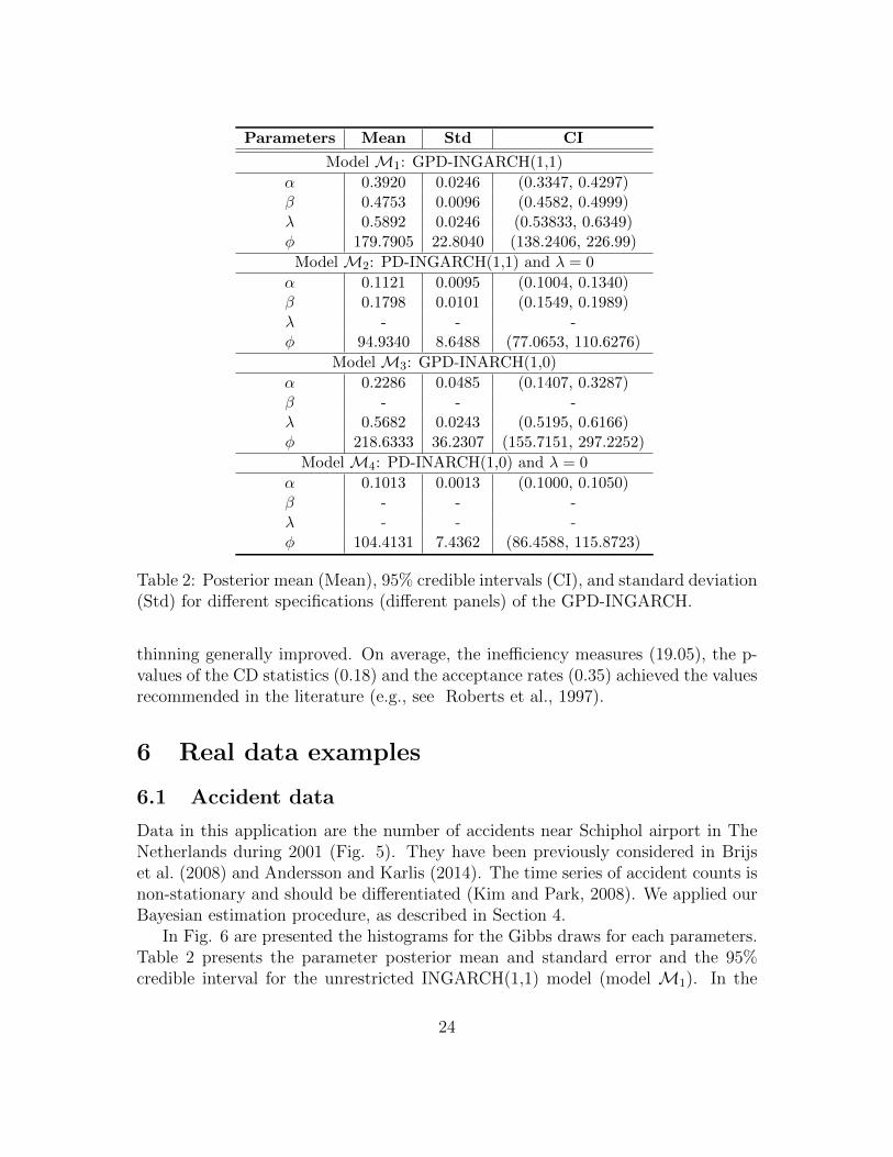
Table 2: Posterior mean (Mean), 95% credible intervals (CI), and standard deviation(Std) for different specifications (different panels) of the GPD-INGARCH.

thinning generally improved. On average, the inefficiency measures (19.05), the p-values of the CD statistics (0.18) and the acceptance rates (0.35) achieved the valuesrecommended in the literature (e.g., see Roberts et al., 1997).

6 Real data examples

6.1 Accident data

Data in this application are the number of accidents near Schiphol airport in TheNetherlands during 2001 (Fig. 5). They have been previously considered in Brijset al. (2008) and Andersson and Karlis (2014). The time series of accident counts isnon-stationary and should be differentiated (Kim and Park, 2008). We applied ourBayesian estimation procedure, as described in Section 4.

In Fig. 6 are presented the histograms for the Gibbs draws for each parameters.Table 2 presents the parameter posterior mean and standard error and the 95%credible interval for the unrestricted INGARCH(1,1) model (model M1). In the

24

0 50 100 150 200 250 300 350

Time

0

5

10

15

20

25

30

0 50 100 150 200 250 300 350

Time

-20

-10

0

10

20

30

Figure 5: Frequency (top) and month-on-month changes (bottom) of the accidentsat the Schiphol airport in The Netherlands in 2001.

α β

λ φ

Figure 6: Histograms of the MCMC draws for the parameters of the Schipol’saccident data of Fig. 5.

25

data, we found evidence of high persistence in the expected accident arrivals, i.e.α+β = 0.8673 and heteroskedastic effects, i.e. β = 0.4753. Also, there is evidence infavour of overdispersion, λ = 0.5892 and overdispersion persistsence φ = 179.7905.We study the contribution of the heteroskedasticy and persistence by testing somerestrictions of the INGARCH(1,1) (models from M2 to M4 in Tab. 2).

Bayesian inference compares models via the so-called Bayes factor, which is theratio of normalizing constants of the posterior distributions of two different models(see Cameron et al. (2014) for a review). MCMC methods allows for generatingsamples from the posterior distributions which can be used to estimate the ratio ofnormalizing constants.

In this paper we use the method proposed by Geyer (1994). The method consistsin deriving the normalizing constants by reverse logistic regression. The idea behindthis method is to consider the different estimates as if they were sampled from amixture of two distributions with probability

pj(x, η) =hj(x) exp(ηj)

h1(x) exp(η1) + h2(x) exp(η2), j = 1, 2 (73)

to be generated from the j-th distribution of the mixture. Geyer (1994) proposedto estimate the log-Bayes factor κ = η2 − η1 by maximizing the quasi-likelihoodfunction

`n(κ) =n∑i=1

log p1(Xi1, η1) +n∑i=1

log p2(Xi2, η2) (74)

where n is the number of MCMC draws for each model and Xij =

log f(Z1:T , X(i)1:T , Y

(i)1:T |θ(i)) is the log-likelihood evaluated at the i-th MCMC sample

for each model of Tab. 2.We performed six reverse logistic regressions, in which we compare pairwise our

models. The approximated logarithmic Bayes factors BF (Mi,Mj) are given in Tab.3. It is possible to see that our GPD-INGARCH(1, 1),M1, is preferable with respectto the other models. Notice that M2 corresponds to an INGARCH(1, 1) wherethe observations are form a standard Poisson-difference model PD-INGARCH(1, 1),M3 corresponds to an autoregressive model, GPD-INARCH(1, 0), whereasM4 is astandard Poisson difference augoregressive model, PD-INARCH(1, 0).

6.2 Cyber threats data

According to the Financial Stability Board (FSB, 2018, pp. 8-9), a cyber incidentis any observable occurrence in an information system that jeopardizes the cybersecurity of the system, or violates the security policies and procedures or the usepolicies. Over the past years there have been several discussions on the taxonomy ofincidents classification (see, e.g. ENISA, 2018), in this paper we use the classification

26

BF(Mi,Mj) M2 M3 M4

M1333.45 25.19 121.44(5.818) (0.253) (0.521)

M2-226.86 -300.96(2.024) (2.522)

M3-73.25(0.358)

Table 3: Logarithmic Bayes Factor, BF(Mi,Mj), of the model Mi (rows) againstmodel Mj (columns), with i < j. Where M1 is the GPD-INGARCH(1,1), M2 isthe PD-INGARCH(1,1) with λ = 0, M3 is the GPD-INARCH(1,0) and M4 is thePD-INARCH(1,0) with λ = 0. Number in parenthesis are standard deviations ofthe estimated Bayes factors.

provided in the Hackmageddon dataset. Hackmageddon is a well-known cyber-incident website that collects public reports and provides the number of cyberincidents for different categories of threats: crimes, espionage and warfare.

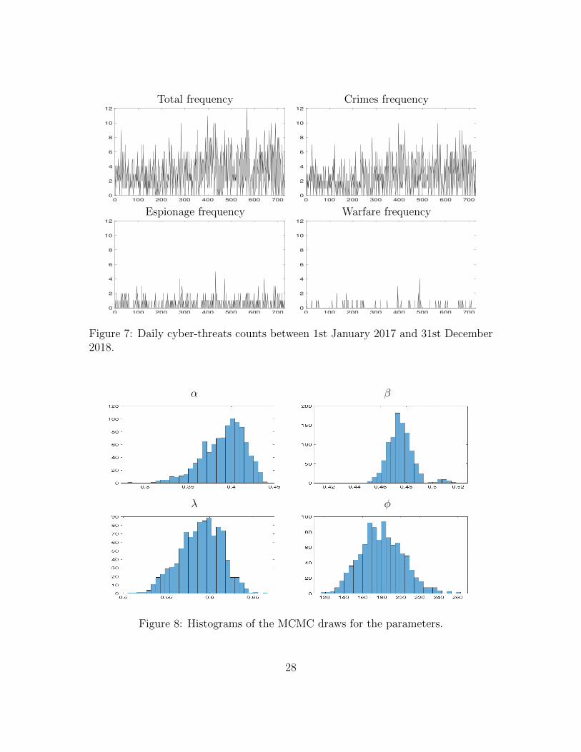
Figure 7 shows the total and category-specific number of cyber attacks at adaily frequency from January 2017 to December 2018. Albeit limited in the varietyof cyber attacks the dataset covers some relevant cyber events and is one of the fewpublicly available datasets (Agrafiotis et al., 2018). The daily threats frequenciesare between 0 and 12 which motivates the use of a discrete distribution. We removethe upward trend by considering the first difference and fit the GPD-INGARCHmodel proposed in Section 2.

We applied our estimation procedure, as described in Section 4. As in theprevious application, we fix α0 = 1.05 that is coherent with the conditional mean ofthe time series. We ran the Gibbs sampler for 110000 iterations, where we discardedthe first 10000 iterations as burn-in sample. In Fig. 8 are presented the histogramsfor the Gibbs draws for each parameters.

Figure 8 shows that, as before, it is reasonable to fit a GPD-INGARCH processto the difference of cyber attacks since both the autoregressive parameter α andβ, that represent the heteroskedastic feature of the data, are different from zero.Additionally, the value of λ suggest the presence of over-dispersion in the data.

Given the importance of forecasting cyber-attacks, in this section we presentthe results of one-step-ahead forecasting exercise over a period of 120. We followan approach based on predictive distributions which quantifies all uncertaintyassociated with the future number of attacks and is used in a wide range ofapplications (see, e.g. McCabe and Martin, 2005; McCabe et al., 2011, andreferences therein). We account for parameter uncertainty and approximate the

predictive distribution by MCMC. At tht j-th MCMC iteration we draw Z(j)T+h from

the conditional distribution given past observations and the parameter draw θ(j)

27

Total frequency Crimes frequency

0 100 200 300 400 500 600 700

0

2

4

6

8

10

12

0 100 200 300 400 500 600 700

0

2

4

6

8

10

12

Espionage frequency Warfare frequency

0 100 200 300 400 500 600 700

0

2

4

6

8

10

12

0 100 200 300 400 500 600 700

0

2

4

6

8

10

12

Figure 7: Daily cyber-threats counts between 1st January 2017 and 31st December2018.

α β

λ φ

Figure 8: Histograms of the MCMC draws for the parameters.

28

100 200 300 400 500 600 700

-20

-15

-10

-5

0

5

10

15

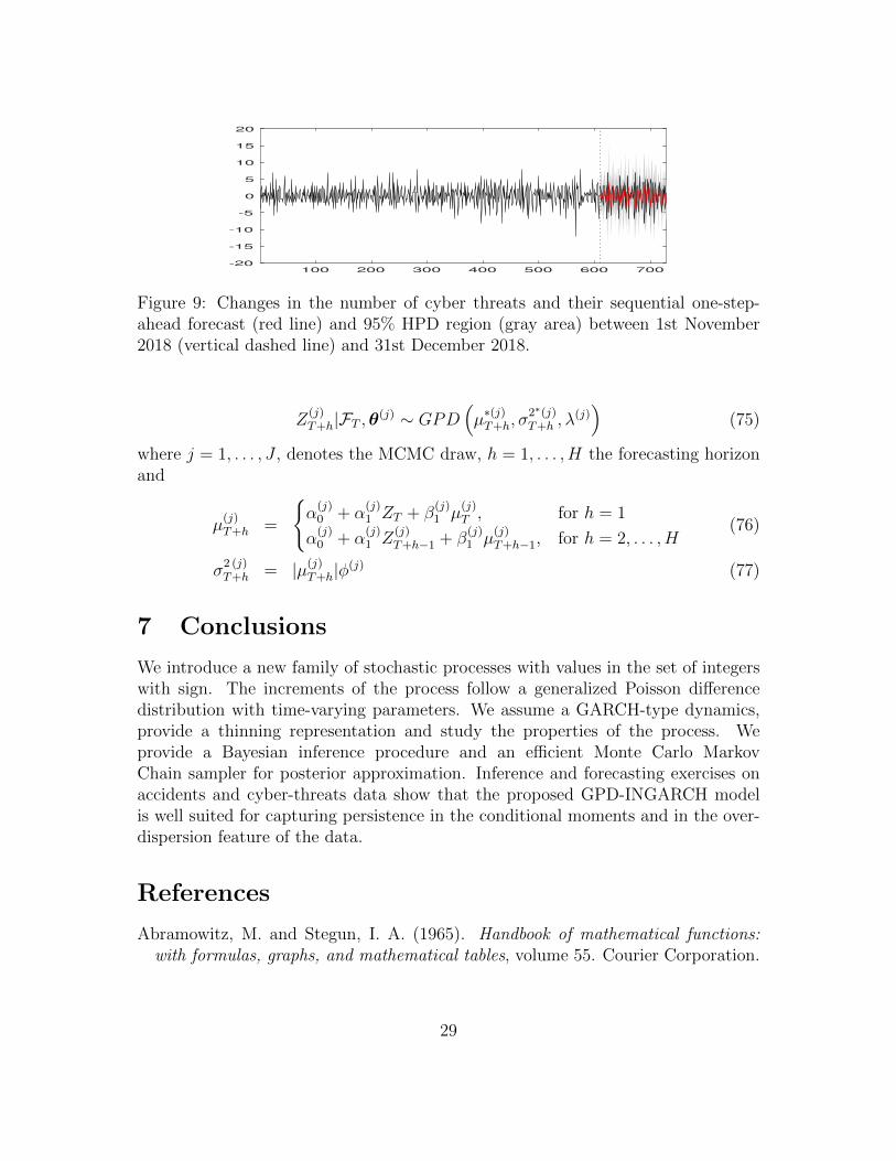
20

Figure 9: Changes in the number of cyber threats and their sequential one-step-ahead forecast (red line) and 95% HPD region (gray area) between 1st November2018 (vertical dashed line) and 31st December 2018.

Z(j)T+h|FT ,θ

(j) ∼ GPD(µ∗(j)T+h, σ

2∗(j)T+h , λ

(j))

(75)

where j = 1, . . . , J , denotes the MCMC draw, h = 1, . . . , H the forecasting horizonand

µ(j)T+h =

α

(j)0 + α

(j)1 ZT + β

(j)1 µ

(j)T , for h = 1

α(j)0 + α

(j)1 Z

(j)T+h−1 + β

(j)1 µ

(j)T+h−1, for h = 2, . . . , H

(76)

σ2 (j)T+h = |µ(j)

T+h|φ(j) (77)

7 Conclusions

We introduce a new family of stochastic processes with values in the set of integerswith sign. The increments of the process follow a generalized Poisson differencedistribution with time-varying parameters. We assume a GARCH-type dynamics,provide a thinning representation and study the properties of the process. Weprovide a Bayesian inference procedure and an efficient Monte Carlo MarkovChain sampler for posterior approximation. Inference and forecasting exercises onaccidents and cyber-threats data show that the proposed GPD-INGARCH modelis well suited for capturing persistence in the conditional moments and in the over-dispersion feature of the data.

References

Abramowitz, M. and Stegun, I. A. (1965). Handbook of mathematical functions:with formulas, graphs, and mathematical tables, volume 55. Courier Corporation.

29

Agrafiotis, I., Nurse, J. R. C., Goldsmith, M., Creese, S., and Upton, D.(2018). A taxonomy of cyber-harms: Defining the impacts of cyber-attacks andunderstanding how they propagate. Journal of Cybersecurity, 4(1).

Al-Osh, M. and Alzaid, A. A. (1987). First-order integer-valued autoregressive(INAR (1)) process. Journal of Time Series Analysis, 8(3):261–275.

Al-Osh, M. A. and Aly, E.-E. A. (1992). First order autoregressive time serieswith negative binomial and geometric marginals. Communications in Statistics -Theory and Methods, 21(9):2483–2492.

Alomani, G. A., Alzaid, A. A., Omair, M. A., et al. (2018). A Skellam GARCHmodel. Brazilian Journal of Probability and Statistics, 32(1):200–214.

Alzaid, A. and Al-Osh, M. (1993). Generalized Poisson ARMA processes. Annalsof the Institute of Statistical Mathematics, 45(2):223–232.

Alzaid, A. A. and Omair, M. A. (2014). Poisson difference integer valuedautoregressive model of order one. Bulletin of the Malaysian MathematicalSciences Society, 37(2):465–485.

Anderson, R. and Moore, T. (2006). The economics of information security. Science,314(5799):610–613.

Andersson, J. and Karlis, D. (2014). A parametric time series model with covariatesfor integers in Z. Statistical Modelling, 14(2):135–156.

Billio, M., Casarin, R., and Osuntuyi, A. (2016). Efficient Gibbs sampling forMarkov switching GARCH models. Computational Statistics and Data Analysis,100:37 – 57.

Bormetti, G., Casarin, R., Corsi, F., and Livieri, G. (2019). A stochastic volatilitymodel with realized measures for option pricing. Journal of Business & EconomicStatistics, 0(0):1–31.

Brenner, S. W. (2004). Cybercrime metrics: Old wine, new bottles? VirginiaJournal of Law and Technology, 9(13):1–53.

Brijs, T., Karlis, D., and Wets, G. (2008). Studying the effect of weather conditionson daily crash counts using a discrete time-series model. Accident Analysis &Prevention, 40(3).

Brockwell, P. J., Davis, R. A., and Fienberg, S. E. (1991). Time Series: Theory andMethods: Theory and Methods. Springer Science & Business Media.

30

Cameron, E., Pettitt, A., et al. (2014). Recursive pathways to marginal likelihoodestimation with prior-sensitivity analysis. Statistical Science, 29(3).

Cardinal, M., Roy, R., and Lambert, J. (1999). On the application of integer-valuedtime series models for the analysis of disease incidence. Statistics in Medicine,18(15):2025–2039.

Casarin, R., Marin, J.-M., et al. (2009). Online data processing: Comparison ofBayesian regularized particle filters. Electronic Journal of Statistics, 3:239–258.

Chen, C. W. and Lee, S. (2016). Generalized Poisson autoregressive models for timeseries of counts. Computational Statistics & Data Analysis, 99:51–67.

Chen, C. W., So, M. K., Li, J. C., and Sriboonchitta, S. (2016). Autoregressiveconditional negative binomial model applied to over-dispersed time series ofcounts. Statistical Methodology, 31:73–90.

Chib, S., Nardari, F., and Shephard, N. (2002). Markov chain Monte Carlo methodsfor stochastic volatility models. Journal of Econometrics, 108(2):281–316.

Consul, P. (1990). On some properties and applications of quasi-binomialdistribution. Communications in Statistics-Theory and Methods, 19(2):477–504.

Consul, P. and Famoye, F. (1986). On the unimodality of generalized Poissondistribution. Statistica neerlandica, 40(2):117–122.

Consul, P. and Famoye, F. (1992). Generalized Poisson regression model.Communications in Statistics-Theory and Methods, 21(1):89–109.

Consul, P. and Mittal, S. (1975). A new urn model with predetermined strategy.Biometrische Zeitschrift, 17(2):67–75.

Consul, P. and Shenton, L. (1975). On the probabilistic structure and properties ofdiscrete Lagrangian distributions. In A modern course on statistical distributionsin scientific work, pages 41–57.

Consul, P. C. (1986). On the differences of two generalized Poisson variates.Communications in Statistics - Simulation and Computation, 15(3):761–767.

Consul, P. C. (1989). Generalized Poisson Distributions. Dekker New York.

Consul, P. C. and Famoye, F. (2006). Lagrangian probability distributions. Springer.

Consul, P. C. and Jain, G. C. (1973). A generalization of the Poisson distribution.Technometrics, 15(4):791–799.

31

Consul, P. C. and Shenton, L. (1973). Some interesting properties of Lagrangiandistributions. Communications in Statistics-Theory and Methods, 2(3):263–272.

Cunha, E. T. d., Vasconcellos, K. L., and Bourguignon, M. (2018). A skewinteger-valued time-series process with generalized Poisson difference marginaldistribution. Journal of Statistical Theory and Practice, 12(4):718–743.

Davis, R. A., Dunsmuir, W. T., and Wang, Y. (1999). Modeling time series of countdata. Statistics Textbooks and Monographs, 158:63–114.

Demirtas, H. (2017). On accurate and precise generation of generalized Poissonvariates. Communications in Statistics-Simulation and Computation, 46(1):489–499.

Edwards, B., Hofmeyr, S. A., and Forrest, S. (2015). Hype and heavy tails: A closerlook at data breaches. J. Cybersecurity, 2:3–14.

EIOPA (2019). Cyber risk for insurers - challenges and opportunities. Availableat https://eiopa.europa.eu/Publications/Reports/EIOPA_Cyber_risk_

for_insurers_Sept2019.pdf.

ENISA (2018). Referenceincident classification taxonomy. Available at https://www.enisa.europa.eu/

publications/reference-incident-classification-taxonomy.pdf.

Famoye, F. (1993). Restricted generalized Poisson regression model.Communications in Statistics-Theory and Methods, 22(5):1335–1354.

Famoye, F. (1997). Generalized Poisson random variate generation. AmericanJournal of Mathematical and Management Sciences, 17(3-4):219–237.

Famoye, F. (2015). A multivariate generalized Poisson regression model.Communications in Statistics-Theory and Methods, 44(3):497–511.

Famoye, F. and Consul, P. (1995). Bivariate generalized Poisson distribution withsome applications. Metrika, 42(1).

Famoye, F., Wulu, J. T., and Singh, K. P. (2004). On the generalized Poissonregression model with an application to accident data. Journal of Data Science,2(2004):287–295.

Ferland, R., Latour, A., and Oraichi, D. (2006). Integer-valued GARCH process.Journal of Time Series Analysis, 27(6):923–942.

32

Francq, C. and Zakoian, J.-M. (2019). GARCH models: structure, statisticalinference and financial applications. Wiley.

Freeland, R. and McCabe, B. P. (2004). Analysis of low count time series data byPoisson autoregression. Journal of Time Series Analysis, 25(5):701–722.

Freeland, R. K. (1998). Statistical analysis of discrete time series with applicationto the analysis of workers’ compensation claims data. PhD thesis, University ofBritish Columbia.

Freeland, R. K. (2010). True integer value time series. AStA Advances in StatisticalAnalysis, 94(3):217–229.

FSB (2018). Cyber lexicon. Available at https://www.fsb.org/wp-content/

uploads/P121118-1.pdf.

Geweke, J. (1992). Evaluating the Accuracy of Sampling-Based Approaches to theCalculation of Posterior Moments. In Bernardo, J. M., Berger, J. O., Dawid,A. P., and Smith, A. F. M., editors, Bayesian Statistics 4, pages 169–193. OxfordUniversity Press, Oxford.

Geyer, C. J. (1994). Estimating normalizing constants and reweighting mixtures.Technical Report 568, School of Statistics, Univ. Minnesota.

Hassanien, A. E., Fouad, M. M., Manaf, A. A., Zamani, M., Ahmad, R.,and Kacprzyk, J. (2016). Multimedia Forensics and Security: Foundations,Innovations, and Applications, volume 115. Springer.

Heinen, A. (2003). Modelling time series count data: An autoregressive conditionalPoisson model. Available at SSRN 1117187.

Hubert Jr, P. C., Lauretto, M. S., and Stern, J. M. (2009). Fbst for generalizedPoisson distribution. In AIP Conference Proceedings, volume 1193, pages 210–217.AIP.

Husak, M., Komarkova, J., Bou-Harb, E., and Celeda, P. (2018). Survey of attackprojection, prediction, and forecasting in cyber security. IEEE CommunicationsSurveys & Tutorials, 21(1):640–660.

Irwin, J. O. (1937). The frequency distribution of the difference between twoindependent variates following the same Poisson distribution. Journal of the RoyalStatistical Society, 100(3):415–416.

Jin-Guan, D. and Yuan, L. (1991). The integer-valued autoregressive (INAR (p))model. Journal of Time Series Analysis, 12(2):129–142.

33

Joe, H. (1996). Time series models with univariate margins in the convolution-closedinfinitely divisible class. Journal of Applied Probability, 33(3):664–677.

Karlis, D. and Ntzoufras, I. (2006). Bayesian analysis of the differences of countdata. Statistics in Medicine, 25(11):1885–1905.

Kedem, B. and Fokianos, K. (2005). Regression models for time series analysis,volume 488. John Wiley & Sons.

Kim, H.-Y. and Park, Y. (2008). A non-stationary integer-valued autoregressivemodel. Statistical Papers, 49(3):485.

Koopman, S. J., Lit, R., and Lucas, A. (2014). The dynamic Skellam model withapplications. WorkingPaper 14-032/IV/DSF73, Tinbergen Institute.

Latour, A. (1998). Existence and stochastic structure of a non-negative integer-valued autoregressive process. Journal of Time Series Analysis, 19(4):439–455.

Liesenfeld, R., Nolte, I., and Pohlmeier, W. (2006). Modelling financial transactionprice movements: A dynamic integer count data model. Empirical Economics,30(4):795–825.

MacDonald, I. L. and Zucchini, W. (1997). Hidden Markov and other models fordiscrete-valued time series, volume 110. CRC Press.

McCabe, B. and Martin, G. (2005). Bayesian predictions of low count time series.International Journal of Forecasting, 21(2):315 – 330.

McCabe, B. P. M., Martin, G. M., and Harris, D. (2011). Efficient probabilisticforecasts for counts. Journal of the Royal Statistical Society: Series B, 73(2):253–272.

McKenzie, E. (1985). Some simple models for discrete variate time series. Journalof the American Water Resources Association, 21(4):645–650.

McKenzie, E. (1986). Autoregressive moving-average processes with negative-binomial and geometric marginal distributions. Advances in Applied Probability,18(3):679?705.

McKenzie, E. (2003). Ch. 16. discrete variate time series. Handbook of statistics,21:573–606.

Passeri, P. (2019). Hackmageddon - information security timelines and statistics.https://www.hackmageddon.com/.

34

Pedeli, X. and Karlis, D. (2011). A bivariate INAR(1) process with application.Statistical modelling, 11(4):325–349.

Robert, C. and Casella, G. (2013). Monte Carlo statistical methods. Springer Science& Business Media.

Roberts, G. O., Gelman, A., Gilks, W. R., et al. (1997). Weak convergence andoptimal scaling of random walk metropolis algorithms. The Annals of AppliedProbability, 7(1):110–120.

Rydberg, T. and Shephard, N. (2000). Bin models for trade-by-trade data. Modellingthe number of trades in fixed interval of time. Paper, 740:28.

Rydberg, T. H. and Shephard, N. (2003). Dynamics of trade-by-trade pricemovements: decomposition and models. Journal of Financial Econometrics,1(1):2–25.

Scotto, M. G., Weiß, C. H., and Gouveia, S. (2015). Thinning-based models in theanalysis of integer-valued time series: A review. Statistical Modelling, 15(6):590–618.

Shahtahmassebi, G. and Moyeed, R. (2014). Bayesian modelling of integer datausing the generalised Poisson difference distribution. International Journal ofStatistics and Probability, 3(1):35.

Shahtahmassebi, G. and Moyeed, R. (2016). An application of the generalizedPoisson difference distribution to the bayesian modelling of football scores.Statistica Neerlandica, 70(3):260–273.

Skellam, J. (1946). The frequency distribution of the difference between two poissonvariates belonging to different populations. Journal of the Royal StatisticalSociety: Series A, 109(Pt 3):296.

Steutel, F. W. and van Harn, K. (1979). Discrete analogues of self-decomposabilityand stability. Annals of Probability, 7(5):893–899.

Tanner, M. A. and Wong, W. H. (1987). The calculation of posterior distributions bydata augmentation. Journal of the American Statistical Association, 82(398):528–540.

Tripathi, R. C., Gupta, P. L., and Gupta, R. C. (1986). Incomplete momentsof modified power series districutions with applications. Communications inStatistics-Theory and Methods, 15(3):999–1015.

35

Wang, W. and Famoye, F. (1997). Modeling household fertility decisions withgeneralized Poisson regression. Journal of Population Economics, 10(3):273–283.

Weiß, C. H. (2008). Thinning operations for modeling time series of counts? Asurvey. Advances in Statistical Analysis, 92(3):319.

Weiß, C. H. (2009). Modelling time series of counts with overdispersion. StatisticalMethods and Applications, 18(4):507–519.

Werner, G., Yang, S., and McConky, K. (2017). Time series forecasting of cyberattack intensity. In Proceedings of the 12th Annual Conference on cyber andinformation security research, page 18. ACM.

Xu, M., Hua, L., and Xu, S. (2017). A vine copula model for predicting theeffectiveness of cyber defense early-warning. Technometrics, 59(4):508–520.

Zamani, H., Faroughi, P., and Ismail, N. (2016). Bivariate generalized Poissonregression model: Applications on health care data. Empirical Economics,51(4):1607–1621.

Zamani, H. and Ismail, N. (2012). Functional form for the generalizedPoisson regression model. Communications in Statistics-Theory and Methods,41(20):3666–3675.

Zeger, S. L. (1988). A regression model for time series of counts. Biometrika,75(4):621–629.

Zhang, H., Wang, D., and Zhu, F. (2010). Inference for INAR(p) processes withsigned generalized power series thinning operator. Journal of Statistical Planningand Inference, 140(3):667–683.

Zheng, H., Basawa, I. V., and Datta, S. (2007). First-order random coefficientinteger-valued autoregressive processes. Journal of Statistical Planning andInference, 137(1):212 – 229.

Zhu, F. (2012). Modeling overdispersed or underdispersed count data withgeneralized Poisson integer-valued GARCH models. Journal of MathematicalAnalysis and Applications, 389(1):58–71.

Zhu, F.-K. and Li, Q. (2009). Moment and Bayesian estimation of parameters inthe INGARCH(1, 1) model. Journal of Jilin University, 47:899–902.

36

A Distributions used in this paper

A.1 Poisson Difference distribution

The Poisson difference distribution, a.k.a. as Skellam distribution, is a discretedistribution defined as the difference of two independent Poisson random variablesN1 − N2, with parameters λ1 and λ2. It has been introduced by Irwin (1937) andSkellam (1946).

The probability mass function of the Skellam distribution for the differenceX = N1 −N2 is

P (X = x) = e−(λ1+λ2)

(λ1

λ2

)x/2I|x|(2

√λ1λ2), with X ∈ Z (A.1)

where Z = . . . ,−1, 0, 1, . . . is the set of positive and negative integer numbers, andIk(z) is the modified Bessel function of the first kind, defined as (Abramowitz andStegun, 1965)

Iv(z) =(z

2

)2∞∑k=0

(z2

4

)kk!Γ(v + k + 1)

(A.2)

It can be used, for example, to model the difference in number of events, likeaccidents, between two different cities or years. Moreover, can be used to modelthe point spread between different teams in sports, where all scored points areindependent and equal, meaning they are single units. Another applications can befound in graphics since it can be used for describing the statistics of the differencebetween two images with a simple Shot noise, usually modelled as a Poisson process.

The distribution has the following properties:

• Parameters: λ1 ≥ 0, λ2 ≥ 0

• Support: −∞,+∞

• Moment-generating function: e−(λ1+λ2)+λ1et+λ2e−t

• Probability generating function: e−(λ1+λ2)+λ1t+λ2/t

• Characteristic function: e−(λ1+λ2)+λ1eit+λ2e−it

• Moments

1. Mean: λ1 − λ2

2. Variance: λ1 + λ2

3. Skewness: λ1−λ2(λ1+λ2)3/2

37

4. Excess Kurtosis: 1λ1+λ2

• The Skellam probability mass function is normalized:∑+∞

k=−∞ p(k;λ1, λ2) = 1

A.2 Generalized Poisson distribution

The Generalized Poisson distribution (GP) has been introduced by Consul and Jain(1973) in order to overcome the equality of mean and variance that characterizes thePoisson distribution. In some cases the occurrence of an event, in a population thatshould be Poissonian, changes with time or dependently on previous occurrences.Therefore, mean and variances are unequal in the data. In different fields a vastnessof mixture and compound distribution have been considered, Consul and Jainintroduced the GP distribution in order to obtain a unique distribution to be usedin the cases said above, by allowing the introduction of an additional parameter.

See Consul and Famoye (2006) for some applications of the Generalized Poissondistribution. Application of the GP distribution can be find as well in economicsand finance. Consul (1989) showed that the number of unit of different commoditiespurchased by consumers in a fixed period of time follows a Generalized Poissondistribution. He gave interpretation of both parameters of the distribution: θ denotethe basic sales potential for the commodity, while λ the average rates of likinggenerated by the product between consumers. Tripathi et al. (1986) provide anapplication of the GP distribution in textile manufacturing industry. In particular,given the established use of the Poisson distribution in the field, they compare thePoisson and the GP distributions when firms want to increase their profit. Theyfound that the Generalized Poisson, considering different values of the parameters,always yield larger profits. Moreover, the Generalized Poisson distribution, asstudied by Consul (1989), can be used to describe accidents of various kinds, such as:shunting accidents, home injuries and strikes in industries. Another application toaccidents has been carried out by Famoye and Consul (1995), where they introduceda bivariate extension to the GP distribution and studied two different estimationmethods, i.e. method of moments and MLE, and the goodness of fit of thedistribution in accidents statistics. Hubert Jr et al. (2009) test for the value of theGP distribution extra parameter by means of a Bayesian hypotheses test procedure,namely the Full Bayesian Significance Test. Famoye (1997) and Demirtas (2017)provided different methods of sampling from the Generalized Poisson distributionand algorithms for sampling. As regard processes, the GP distribution has beenused in different models. For example, Consul and Famoye (1992) introducedthe GP regression model, while Famoye (1993) studied the restricted generalizedPoisson regression. Wang and Famoye (1997) applied the GP regression model tohouseholds’ fertility decisions and Famoye et al. (2004) carried out an applicationof the GP regression model to accident data. Zamani and Ismail (2012) develop a

38

functional form of the GP regression model, Zamani et al. (2016) introduced a fewforms of bivariate GP regression model and different applications using dataset onhealthcare, in particular the Australian health survey and the US National MedicalExpenditure survey. Famoye (2015) provide a multivariate GP regression model,based on a multivariate version of the GP distribution, and two applications: to thehealthcare utilizations and to the number of sexual partners.

The Generalized Poisson distribution of a random variable X with parameters θand λ is given by

Px(θ, λ) =

θ(θ+λx)x−1

x!e(−θ−λx), x = 0, 1, 2, . . .

0, for x > m if λ < 0.(A.3)

The GP is part of the class of general Lagrangian distributions. The GP hasGenerating functions and moments

• Parameters:

1. θ > 0

2. max(−1,−θ/m) ≤ λ ≤ 1

3. m(≥ 4) is the largest positive integer for which θ +mλ > 0 when λ < 0

• Moment generating function (mgf): Mx(β) = eθ(es−1), where z = es and u = eβ

• Probability generating function (pgf): G(u) = eθ(z−1), where z = ueλ(z−1)

• Moments:

1. Mean: µ = θ(1− λ)−1

2. Variance: σ2 = θ(1− λ)−3

3. Skewness: β1 = 1+2λ√θ(1−λ)

4. Kurtosis: β2 = 3 + 1+8λ+6λ2

θ(1−λ)

The pgf of the GP is derived by Consul and Jain (1973) by means of the Lagrangeexpansion, namely:

z =∞∑x=1

ux

x!Dx−1(g(z))xz=0 (A.4)

f(z) =∞∑x=0

ux

x!Dx−1(g(z))xf ′(z)|z=0

= f(0) +∞∑x=1

ux

x!Dx−1(g(z))xf ′(z)|z=0

(A.5)

39

where Dx−1 = dx−1

dzx−1 . In particular, for the GP distribution we have (Consul andFamoye, 2006) :

f(z) = eθ(z−1) and g(z) = eλ(z−1) (A.6)

Now, by setting G(u) = f(z) we have the expression above for the pgf. (see proofin

Properties Consul and Jain (1973), Consul (1989), Consul and Famoye (1986)and Consul and Famoye (2006) derived some interesting properties of theGeneralized Poisson distribution.

Theorem 1 (Convolution Property). The sum of two independent randomGeneralized Poisson variates, X + Y , with parameters (θ1, λ) and (θ2, λ) is aGeneralized Poisson variate with parameters (θ1 + θ2, λ).

For a proof of Th. 1 see Consul and Jain (1973).

Theorem 2 (Unimodality). The GP distribution models are unimodal for allvalues of θ and λ and the mode is at x = 0 if θe−λ < 1 and at the dual points x = 0and x = 1 when θe−λ = 1 and for θe−λ > 1 the mode is at some point x = M suchthat:

(θ − e−λ)(eλ − 2λ)−1 < M < a (A.7)

where a is the smallest value of M satisfying the inequality

λ2M2 +M [2λθ − (θ + 2λ)eλ] > 0 (A.8)

For a proof of Th. 2 see Consul and Famoye (1986).Consul and Shenton (1975) and Consul (1989) derived some recurrence relations

between noncentral moments µ′k and the cumulants Kk:

(1− λ)µ′k+1 = θµ′k + θ∂µ′k∂θ

+ λ∂µ′k∂λ

, k = 0, 1, 2, . . . (A.9)

(1− λ)Kk+1 = λ∂Kk

∂λ+ θ

∂Kk

∂θ+, k = 1, 2, 3, . . . . (A.10)

Moreover, a recurrence relation between the central moments of the GPdistribution has been derived:

µk+1 =θk

(1− λ)3µk−1 +

1

1− λ

d µk(t)

dt

t=1

, k = 1, 2, 3, . . . (A.11)

where µk(t) is the central moment µk with θt and λt in place of θ and λ.

40

A.3 Generalized Poisson Difference distribution

The random variable X follows a Generalized Poisson distribution (GP) Px(θ, λ) ifand only if

Px(θ, λ) =θ(θ + xλ)x−1

x!e−θ−xλ x = 0, 1, 2, . . . (A.12)

with θ > 0 and 0 ≤ λ < 1.Let X ∼ Px(θ1, λ) and Y ∼ Py(θ2, λ) be two independent random variables,

Consul (1986) showed that the probability distribution of D, D = X − Y , is:

P (D = d) = e−θ1−θ2−dλ∞∑y=0

θ2(θ2 + yλ)y−1

y!

θ1(θ1 + (y + d)λ)y+d−1

(y + d)!e−2yλ (A.13)

where d takes all integer values in the interval (−∞,+∞). As for the GPdistribution, we need to set lower limits for λ in order to ensure that there areat least five classes with non-zero probability when λ is negative. Hence, we set

max(−1,−θ1/m1) < λ < 1

max(−1,−θ2/m2) < λ < 1

where, m1,m2 ≥ 4 are the largest positive integers such that θ1 + m1λ > 0 andθ2 +m2λ > 0.

Proposition 10. The probability distribution in (A.13) can be written as

P (D = d) = e−(θ1+θ2)·e−dλ∞∑y=0

θ1θ2

y!(y + d)!(θ2+yλ)y−1(θ1+(y+d)λ)y+d−1·e−2yλ = Cd(θ1, θ2, λ).

(A.14)

Therefore, equation (A.14) is the pgf of the difference of two GP variates, fromwhich is possible to obtain the following particular cases:

Cd(θ1, 0, λ) = θ1(θ1+dλ)d−1

d!e−θ1−dλ, for d = 0, 1, 2, . . .

Cd(0, θ2, λ) = θ2(θ2−dλ)−d−1

(−d)!e−θ2+dλ, for d = 0,−1,−2, . . .

Cd(θ1, θ2, 0) = e−θ1−θ2(θ1)d/2(θ2)−d/2Id(2√θ1θ2),

(A.15)

where d is any integer (positive, 0 or negative) and Id(z) is the modified Besselfunction of the first kind, of order d and argument z.

The last result in equation (A.15) is the Skellam distribution (Skellam, 1946).Therefore, the Skellam distribution is a particular case of the difference of two GPvariates.

41

By Consul and Shenton (1973):

G1(u) = eθ1(t1−1) , where t1 = ueλ(t1−1)

andG2(u) = eθ2(t2−1 , where t2 = u−1eλ(t2−1).

Therefore, given that G(u) = G1(u)G2(u), the probability generating function (pgf)of the random variable D = X − Y is

G(u) = exp[(θ1(t1 − 1) + (θ2(t2 − 1)]. (A.16)

From the cumulant generating function

ψ(β) =(T1 − β)θ1

λ+

(T2 + β)θ2

λ

where T1 = β + λ(eT1 − 1) and T2 = −β + λ(eT2 − 1), it is possible to define themean,variance, skewness and kurtosis of the distribution.

L1 =(θ1 − θ2)

1− λis the first cumulant and the mean. (A.17)

L2 =(θ1 + θ2)

(1− λ)3is the second cumulant and the variance. (A.18)

β1 =(θ1 − θ2)2

(θ1 + θ2)3

(1 + 2λ)2

1− λis the skewness. (A.19)

β2 = 3 +1 + 8λ+ 6λ2

(θ1 + θ2)(1− λ)is the kurtosis. (A.20)

In Fig. A.1-A.2, we show the GPD for various setting of λ, σ2 and µ.

42

(a) GPD for µ = −4 and σ2 = 8 (b) GPD for µ = 4 and σ2 = 8

-40 -20 0 20 40

z

0

0.02

0.04

0.06

0.08

0.1

0.12

0.14

Pro

babili

ty

=0.1

=0.2

=0.3

=0.4

-40 -20 0 20 40

z

0

0.02

0.04

0.06

0.08

0.1

0.12

0.14

Pro

babili

ty

=0.1

=0.2

=0.3

=0.4

(c) GPD for µ = 2 and σ2 = 5 (d) GPD for µ = 2 and σ2 = 15

-40 -20 0 20 40

z

0

0.02

0.04

0.06

0.08

0.1

0.12

0.14

0.16

Pro

babili

ty

=0.1

=0.2

=0.3

=0.4

-40 -20 0 20 40

z

0

0.02

0.04

0.06

0.08

0.1P

robabili

ty

=0.1

=0.2

=0.3

=0.4

Figure A.1: Generalized Poisson difference distribution for different values of λ.Panels (a) and (b) show the GPD when λ varies, for a fixed value of σ2 = 8 and twodifferent values of µ. Panels (c) and (d) show the GPD when λ varies, for a fixedvalue of µ = 2 and two different value of σ2.

43

(a) GPD for different values of µ (b) GPD for different values of σ2

-40 -20 0 20 40

z

0

0.02

0.04

0.06

0.08

0.1

Pro

babili

ty

=-14

=-11

=-8

=-5

=5

=8

=11

=14

-30 -20 -10 0 10 20 30

z

0

0.05

0.1

0.15

0.2

0.25

Pro

babili

ty

2=3

2=5

2=7

2=9

2=11

2=13

2=15

Figure A.2: Generalized poisson difference distribution for different values of µ andσ and fixed λ. In panel (a) µ varies, while σ2 = 15 and λ = 0.1 are fixed. In panel(b) σ2 varies and µ = 1 and λ = 0.1 are fixed.

Figure A.1 shows how the GPD distribution varies when λ varies. Given theconstraints imposed to the parameters (see section 2) here λ = (0, 0.1, 0.2, 0.3, 0.4)since smaller values and, possibly, negative values do not met the conditions for theselected values of θ1 and θ2. From panel (a) and especially in panel (b) can be seenthat when λ increases the distribution becomes longer tailed. From panel (c) and(d) we can see that for fixed values µ, when λ decreases, the GPD is more skewedrespectively to the right for µ > 0 (θ1 > θ2) and to the left for µ < 0 (θ1 < θ2).Therefore, the sign of µ determines the skewness of the GPD.

From figure A.2 we can see again, that for positive values of µ the distributionbecomes more right-skewed, panels (a) and (b), and more left-skewed for negativevalues of µ in panels (c) and (d). Moreover, here can be seen better that has θ1

increases the distribution has longer tails.

A.4 Quasi-Binomial distribution

A first version of the Quasi-Binomial distribution, defined as QB-I by Consul andFamoye (2006), was investigated by Consul (1990) as an urn model. In theirdefinition of the QB thinning, however, Alzaid and Al-Osh (1993) used the QBdistribution introduced in the literature by Consul and Mittal (1975) and definedbyConsul and Famoye (2006) as QB-II.

P (X = x) =

(n

x

)ab

a+ b

(a+ xθ)x−1(b+ nθ − xθ)n−x−1

(a+ b+ nθ)n−1(A.21)

44

for x = 0, 1, 2, . . . , n and zero otherwise. where a > 0, b > 0 and θ > −a/n.However, Alzaid and Al-Osh (1993), when defining the QB thinning operator, useda particular case of the QB-II distribution:

P (X = x) = pq

(n

x

)(p+ xθ)x−1(q + (n− x)θ)n−x−1

(1 + nθ)n−1(A.22)

where a = p, q = b, 0 < q = 1− p < 1 and θ is such that nθ < min(p, q). We denotethe QB-II with QB(p,θ,n). For large n, such that np → λ, the QB distributiontends to the Generalized Poisson distribution.

The quasi-binomial (QB) thinning has been introduced by Alzaid and Al-Osh(1993) as a generalization of the binomial thinning to model processes with GPdistribution marginals. Unlike the binomial thinning, the QB thinning is able toobtain the distribution of the corresponding innovation. In particular, the authorsargued in many counting process is more suitable to consider that the probability ofretaining an element may depend on the time and/or the number of already retainedelements. They assumed that, at time t, the number of retained elements follows aQB distribution. Using the notation in Weiß (2008), the QB thinning is defined asfollows:

Proposition 11 (Quasi-Binomial Thinning). Let ρθ,λ be the quasi-binomialthinning operator such that ρθ,λ follows a QB(ρ,θ/λ,x). If X follows a GP(λ,θ)distribution and the quasi-binomial thinning is performed independently on X, thenρθ,λ X has a GP(ρλ,θ) distribution.

The thinned variable, ρθ,λ X, can be interpreted as the number of survivorsfrom a population described by X.

Properties

• Expected value: E[ρθ,λ X] = ρ · µX

• Covariance: E[ρθ,λ X,X] = ρ · σ2X

B Proofs of the results of the paper

B.1 Convolution property of the Generalized Poissondistribution in Section A

Proof of Lemma 1. Let X ∼ GPD(θ1, θ2, λ) and Y ∼ GPD(θ3, θ4, λ). We can writeeach r.v. as

X = X1 −X2 and Y = Y1 − Y2 (B.1)

45

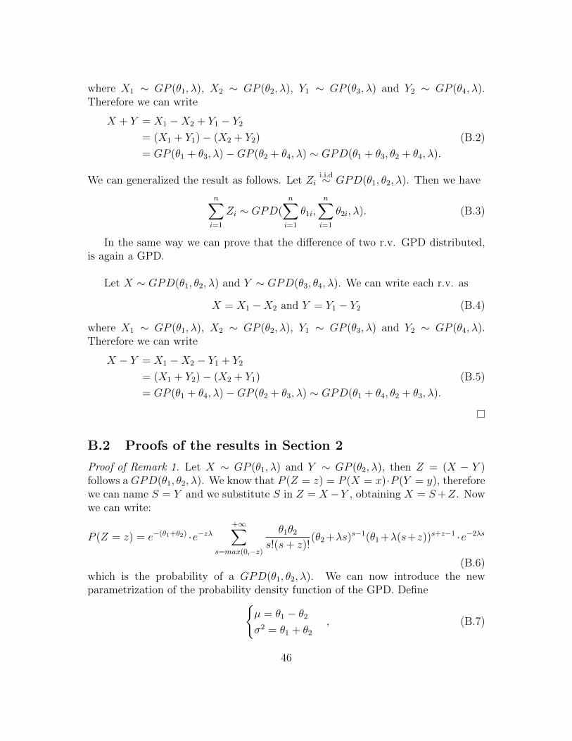
where X1 ∼ GP (θ1, λ), X2 ∼ GP (θ2, λ), Y1 ∼ GP (θ3, λ) and Y2 ∼ GP (θ4, λ).Therefore we can write

X + Y = X1 −X2 + Y1 − Y2

= (X1 + Y1)− (X2 + Y2)

= GP (θ1 + θ3, λ)−GP (θ2 + θ4, λ) ∼ GPD(θ1 + θ3, θ2 + θ4, λ).

(B.2)

We can generalized the result as follows. Let Zii.i.d∼ GPD(θ1, θ2, λ). Then we have

n∑i=1

Zi ∼ GPD(n∑i=1

θ1i,

n∑i=1

θ2i, λ). (B.3)

In the same way we can prove that the difference of two r.v. GPD distributed,is again a GPD.

Let X ∼ GPD(θ1, θ2, λ) and Y ∼ GPD(θ3, θ4, λ). We can write each r.v. as

X = X1 −X2 and Y = Y1 − Y2 (B.4)

where X1 ∼ GP (θ1, λ), X2 ∼ GP (θ2, λ), Y1 ∼ GP (θ3, λ) and Y2 ∼ GP (θ4, λ).Therefore we can write

X − Y = X1 −X2 − Y1 + Y2

= (X1 + Y2)− (X2 + Y1)

= GP (θ1 + θ4, λ)−GP (θ2 + θ3, λ) ∼ GPD(θ1 + θ4, θ2 + θ3, λ).

(B.5)

B.2 Proofs of the results in Section 2

Proof of Remark 1. Let X ∼ GP (θ1, λ) and Y ∼ GP (θ2, λ), then Z = (X − Y )follows a GPD(θ1, θ2, λ). We know that P (Z = z) = P (X = x)·P (Y = y), thereforewe can name S = Y and we substitute S in Z = X−Y , obtaining X = S+Z. Nowwe can write:

P (Z = z) = e−(θ1+θ2) ·e−zλ+∞∑

s=max(0,−z)

θ1θ2

s!(s+ z)!(θ2 +λs)s−1(θ1 +λ(s+z))s+z−1 ·e−2λs

(B.6)which is the probability of a GPD(θ1, θ2, λ). We can now introduce the newparametrization of the probability density function of the GPD. Define

µ = θ1 − θ2

σ2 = θ1 + θ2

, (B.7)

46

thus, we can rewrite both parameters θi, i = 1, 2, with respect to µ and σ2:θ1 = σ2+µ

2

θ2 = σ2−µ2

(B.8)

By substituting B.8 into equation B.6 we have

P (Z = z) = e(σ2+µ2

+σ2−µ2

)e−zλ+∞∑

s=max(0,−z)

(σ2+µ

2

)(σ2−µ

2

)s!(s+ z)!

[σ2 + µ

2+ (s+ z)λ

]s+z−1

[σ2 − µ

2+ sλ

]s−1

e−2λs (B.9)

Carrying out the operations in Eq. B.9 we obtain Eq. B.7.

Proof of Remark 2. If Z ∼ GPD(θ1, θ2, λ) in the parametrization of Consul (1986),the moments are given in equations A.17-A.20. By using our reparametrization ofthe GDP

θ1 =σ2 + µ

2, θ2 =

σ2 − µ2

(B.10)

in equations A.17-A.20, we obtain

E(Z) =θ1 − θ2

1− λ=

µ

1− λ(B.11)

V (Z) =θ1 + θ2

(1− λ)3=

σ2

(1− λ)3= κ2 (B.12)

S(Z) =µ(3)

σ3=

κ3

κ3/22

=µ(1 + 2λ)

(1− λ)5

((1− λ)3

σ2

)3/2

=µ

σ3

(1 + 2λ)√1− λ

(B.13)

K(Z) =κ4 + 3κ2

2

σ4

=

(σ2(1 + 8λ+ 6λ2)

(1− λ)7+

3σ4

(1− λ)6

)((1− λ)6

σ4

)= 3 +

1 + 8λ+ 6λ2

σ2(1− λ)

(B.14)

where κi, i = 2, 3, 4 are respectively the second, third and fourth cumulants.

47

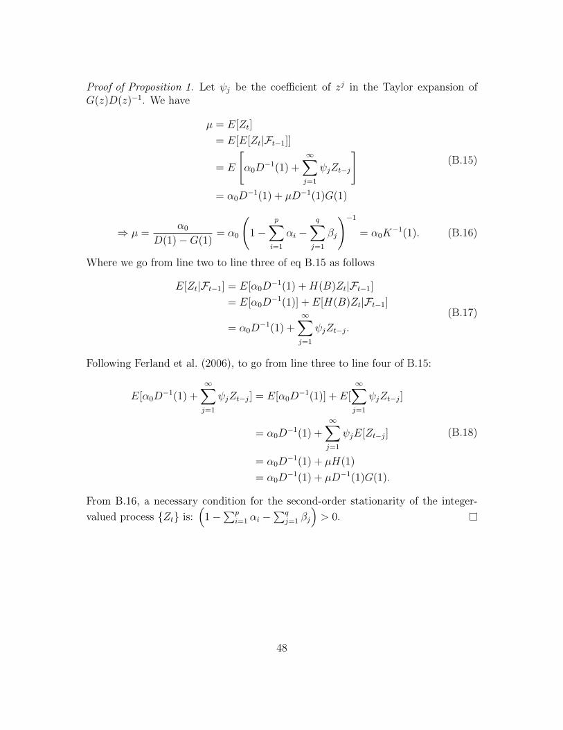
Proof of Proposition 1. Let ψj be the coefficient of zj in the Taylor expansion ofG(z)D(z)−1. We have

µ = E[Zt]

= E[E[Zt|Ft−1]]

= E

[α0D

−1(1) +∞∑j=1

ψjZt−j

]= α0D

−1(1) + µD−1(1)G(1)

(B.15)

⇒ µ =α0

D(1)−G(1)= α0

(1−

p∑i=1

αi −q∑j=1

βj

)−1

= α0K−1(1). (B.16)

Where we go from line two to line three of eq B.15 as follows

E[Zt|Ft−1] = E[α0D−1(1) +H(B)Zt|Ft−1]

= E[α0D−1(1)] + E[H(B)Zt|Ft−1]

= α0D−1(1) +

∞∑j=1

ψjZt−j.

(B.17)

Following Ferland et al. (2006), to go from line three to line four of B.15:

E[α0D−1(1) +

∞∑j=1

ψjZt−j] = E[α0D−1(1)] + E[

∞∑j=1

ψjZt−j]

= α0D−1(1) +

∞∑j=1

ψjE[Zt−j]

= α0D−1(1) + µH(1)

= α0D−1(1) + µD−1(1)G(1).

(B.18)

From B.16, a necessary condition for the second-order stationarity of the integer-

valued process Zt is:(

1−∑p

i=1 αi −∑q

j=1 βj

)> 0.

48

B.3 Proof of the results in Section 3

Proof of Proposition 3.

Z(n)t = X

(n)t − Y

(n)t

= (1− λ)U1t + (1− λ)n∑i=1

ϕ(t−i)1i X(n−i)

t−i − (1− λ)U2t − (1− λ)n∑i=1

ϕ(t−i)2i Y (n−i)

t−i

= (1− λ)(U1t − U2t) + (1− λ)n∑i=1

[(ϕ

(t−i)1i X(n−i)

t−i )− (ϕ(t−i)2i Y (n−i)

t−i )]

= (1− λ)Ut + (1− λ)n∑i=1

ϕ(t−i)i Z(n−i)

t−i .

Proof of Proposition 4. In order to prove the almost sure convergence of Z(n)t we

will prove that the difference of two sequences X(n)t and Y (n)

t that have analmost sure convergence, will have an almost sure convergence.We know that Z

(n)t = X

(n)t − Y

(n)t , where X

(n)t and Y

(n)t are two sequences of GP

random variable. From Zhu (2012) we have

Xn(ω)a.s.−→ X(ω) =⇒ P(ω : lim

n→∞Xn(ω) = X(ω)) = 1

andYn(ω)

a.s.−→ Y (ω) =⇒ P(ω : limn→∞

Yn(ω) = Y (ω)) = 1.

LetA = ω : lim

n→∞Xn(ω) = X(ω)

and

B = ω ∈ Ω× Ω : limn→∞

(aXn(ω) + bYn(ω)) = aX(ω) + bY (ω), ∀a, b ∈ R.

Now we show the almost sure convergence of the sum (aXn(ω) + bYn(ω)).

49

∫Ω

IB(ω)dP(ω) =

∫(Ω∩A)∪(Ω∩AC)

IB(ω)dP(ω)

=

∫Ω

IB(ω)IA(ω)dP(ω) +

∫Ω

IB(ω)IAC (ω)dP(ω)

=

∫Ω

IB(ω)IA(ω)dP(ω) +

∫Ω

IAC (ω)

(∫Ω

IB∩AC (ω)dP(ω|ω′))dP(ω′)

= P(B|A)P(A) + P(B|AC)P(AC)︸ ︷︷ ︸=0

= P(ω : limn→∞

(aXn(ω) + bYn(ω)) = aX(ω) + bY (ω)|A)P(A)︸ ︷︷ ︸=1

= P(ω : a limn→∞

Xn(ω) = aX(ω)− bY (ω) + bY (ω)) = 1

(B.19)

Therefore, if X(ω)n

a.s.−→ X(ω) and Y(ω)n

a.s.−→ Y (ω)

⇒ aXn(ω) + bYn(ω)a.s.−→ aX(ω) + bY (ω), ∀a, b ∈ R.

∀a, b ∈ R. Hence, for a = 1 and b = −1, this is true for the differenceZ

(n)t = X

(n)t − Y

(n)t .

Proof of Proposition 5. We use again the fact that Z(n)t = X

(n)t − Y

(n)t and the

following lemma.

Lemma 2. If Xn(ω) and Yn(ω) have a mean-square limit

Xn(ω)L2

−→ X(ω)

Yn(ω)L2

−→ Y (ω) (B.20)

also their sum will have a mean-square limit.

aXn(ω) + bYn(ω)L2

−→ aX(ω) + bY (ω), ∀a, b ∈ R (B.21)

Hence, by setting a = 1 and b = −1 we will obtain that Lemma 2 will be validalso for the difference of two sequences

Xn(ω)− Yn(ω)L2

−→ X(ω)− Y (ω) (B.22)

and we can say that Z(n)t converges to Zt in L2(Ω,F ,P).

50

Proof of Proposition 6.

gZ(t) = E

[k∏i=1

tZii

]= E

[k∏i=1

tXii

]E

[k∏i=1

1

tYii

]= gX(t)gY(t−1) (B.23)

Proof of Proposition 9. As said before, Z(n)t = X

(n)t − Y

(n)t . Where X

(n)t and Y

(n)t

are finite sums of independent Generalized Poisson variables and it follows that Z(n)t

is a finite sum of Generelized Poisson difference variables. As shown by Zhu (2012),the first two moments of Xt and Yt are finite: E[Xt] = µX ≤ C1, E[Yt] = µY ≤ C ′1,V [Xt] = σ2

X ≤ C2, V [Yt] = σ2Y ≤ C ′2, therefore,

E[Zt] = E[Xt]− E[Yt] = µX − µY ≤ µX + µY ≤ C1 + C ′1 (B.24)

is finite and

V [Xt − Yt] = V [Xt] + V [Xt] = σ2X + σ2

Y ≤ C2 + C ′2 (B.25)

is also finite, where Cov(Xt, Yt) = 0 given that Xt and Yt are independent and whereCi and C ′i, with i = 1, 2 are constants.

Proof of the results in Example 1. For k ≥ 2:

γZ(k) = α1γZ(k − 1) = αk−11 γZ(1) (B.26)

For k = 1:

γZ(1) = Cov(Zt, Zt−1 = α1γZ(0) = α1V (Zt = α1[φ3E(σ2∗

t )] + α1V (µt). (B.27)

For k ≥ 1 we haveγµ(k) = α1γµ(k − 1) = αk1V (µt). (B.28)

For k = 0:

γµ(k) = V (µt) = α1γZ(1)

= α1

α1[φ3E(σ2∗

t ) + V (µt)]

= α21[φ3E(σ2∗

t )] + α21V (µt)

(B.29)

Therefore,

V (µt) =α2

1[φ3E(σ2∗t )]

1− α21

(B.30)

and

V (Zt) = φ3E(σ2∗

t ) + V (µt)

= φ3E(σ2∗

t ) +α2

1[φ3E(σ2∗t )]

1− α21

=φ3E(σ2∗

t )

1− α21

(B.31)

51

where φ = 11−λ . Finally, the autocorrelations are derived as follows:

ρµ(k) =γµ(k)

V (µt)=αk1 V (µt)

V (µt)= αk1 (B.32)

ρZ(k) =γZ(k)

V (Zt)= αk−1

1 γZ (1)1− α2

1

φ3E(σ2∗t )

= αk−11

α1(1− α21)φ3E(σ2∗

t ) + α31φ

3E(σ2∗t )

1− α21

1− α21

φ3E(σ2∗t )

= αk1

(B.33)

Proof of the results in Example 2. For k ≥ 2:

γZ(k) = α1γZ(k − 1) + β1γZ(k − 1) = (α1 + β1)k−1γZ(1) (B.34)

For k = 1:

γZ(1) = Cov(Zt, Zt−1) = α1γZ(0) + β1γµ(0)

= α1V (Zt) + β1V (µt) = α1[φ3E(σ2∗

t )] + (α1 + β1)V (µt).(B.35)

For k ≥ 1 we have

γµ(k) = α1γµ(k − 1) + β1γµ(k − 1) = (α1 + β1)kV (µt). (B.36)

For k = 0:

γµ(k) = V (µt) = α1γZ(1) + β1γµ(1)

= α1

α1[φ3E(σ2∗

t )] + (α1 + β1)V (µt)

+ β1 [(α1 + β1)V (µt)]

= α21[φ3E(σ2∗

t )] + (α1 + β1)2V (µt)

(B.37)

Therefore,

V (µt) =α2

1[φ3E(σ2∗t )]

1− (α1 + β1)2(B.38)

and

V (Zt) = φ3E(σ2∗

t ) + V (µt) = φ3E(σ2∗

t ) +α2

1[φ3E(σ2∗t )]

1− (α1 + β1)2

=φ3E(σ2∗

t )[1− (α1 + β1)2 + α21]

1− (α1 + β1)2

(B.39)

where φ = 11−λ . The autocorrelations are derived as follows:

ρµ(k) =γµ(k)

V (µt)=

(α1 + β1)k V (µt)

V (µt)= (α1 + β1)k (B.40)

52

ρZ(k) =γZ(k)

V (Zt)= (α1 + β1)k−1 γZ (1)

1− (α1 + β1)2

φ3E(σ2∗t )[1− (α1 + β1)2 + α2

1]

= (α1 + β1)k−1 α1[1− β1(α1 + β1)]

1− (α1 + β1)2 + α21

(B.41)

C Numerical Illustration

We consider 400 samples from a two GPD-INGARCH(1,1) and two simulationsettings: one with low persistence and the other with high persistence. The firstsetting has parameters λ = 0.4, α1 = 0.25, β1 = 0.23, α0 = −0.2 and φ = 22.78,while the second setting with parameters λ = 0.6,α1 = 0.53, β1 = 0.25, α0 = −0.2and φ = 26.25. We run the Gibbs sampler for 1,010,000 iterations, discard thefirst 10,000 draws to avoid dependence from initial conditions, and finally applya thinning procedure with a factor of 100 to reduce the dependence betweenconsecutive draws.

The following figures show the posterior approximation of α1,β1 and λ. Forillustrative purposes we report in Fig. C.1-C.3 the MCMC output for one MCMCdraw before removing the burn-in sample and thinning, while in Fig.C.4-C.6 theMCMC output after removing the burn-in sample and thinning.

53

C.1 Before thinning

(a) Low persistence (b) High persistence

0 2 4 6 8 10

nGibbs 105

0.2

0.25

0.3

0.35

0.4

alp

haG

ibbs

0 2 4 6 8 10

nGibbs 105

0.2

0.3

0.4

0.5

0.6

0.7

alp

haG

ibbs

0 2 4 6 8 10

nGibbs 105

0.1

0.15

0.2

0.25

0.3

0.35

0.4

beta

Gib

bs

0 2 4 6 8 10

nGibbs 105

0.1

0.2

0.3

0.4

0.5

0.6

beta

Gib

bs

0 2 4 6 8 10

nGibbs 105

0.25

0.3

0.35

0.4

0.45

lam

bdaG

ibbs

0 2 4 6 8 10

nGibbs 105

0.54

0.56

0.58

0.6

0.62

0.64

0.66

lam

bdaG

ibbs

Figure C.1: MCMC plot for the parameters in the two setting: low persistence andhigh persistence.

54

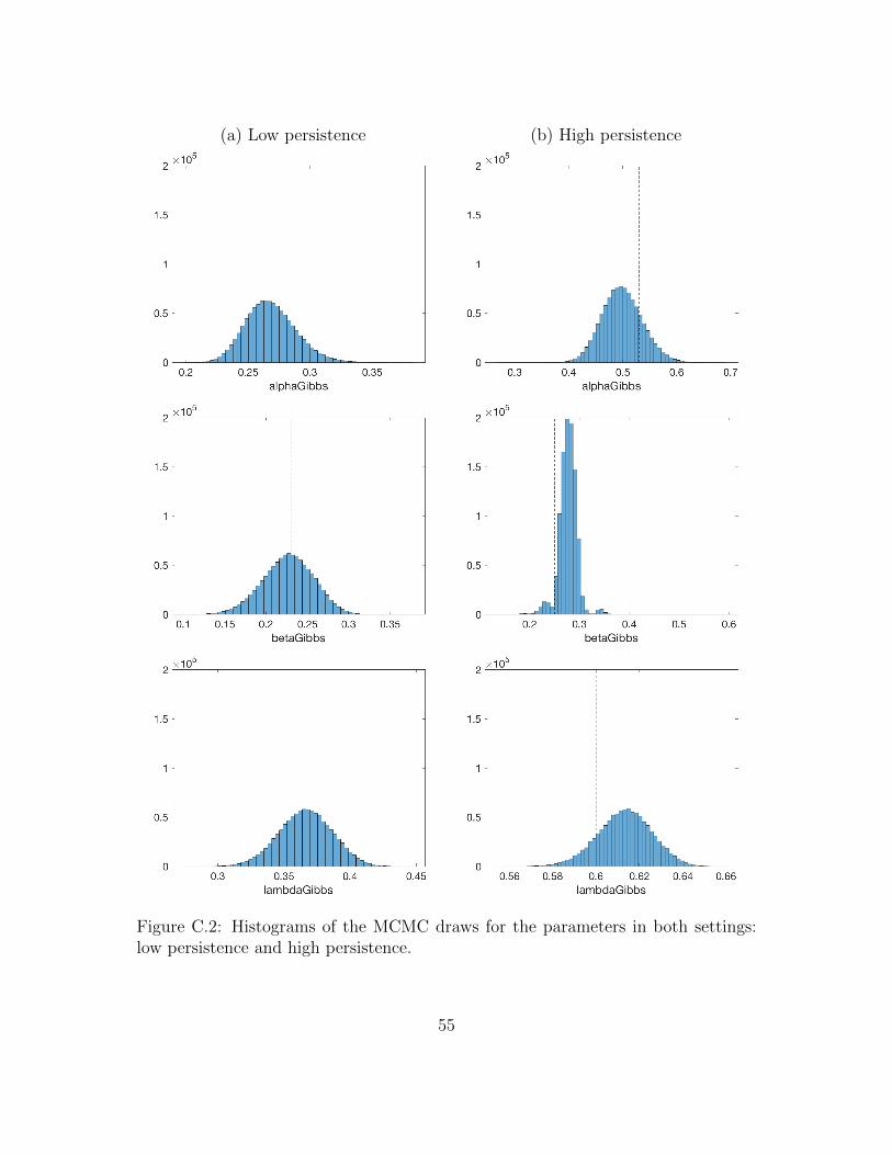
(a) Low persistence (b) High persistence

Figure C.2: Histograms of the MCMC draws for the parameters in both settings:low persistence and high persistence.

55

(a) Low persistence (b) High persistenceα α

-0.2

0

0.2

0.4

0.6

0.8

1

AC

F

0 5 10 15 20

Lag

-0.2

0

0.2

0.4

0.6

0.8

1

AC

F

0 5 10 15 20

Lag

β β

-0.2

0

0.2

0.4

0.6

0.8

1

AC

F

0 5 10 15 20

Lag

-0.2

0

0.2

0.4

0.6

0.8

1

AC

F

0 5 10 15 20

Lag

λ λ

-0.2

0

0.2

0.4

0.6

0.8

1

AC

F

0 5 10 15 20

Lag

-0.2

0

0.2

0.4

0.6

0.8

1

AC

F

0 5 10 15 20

Lag

Figure C.3: Autocorrelation function for the parameters in both low persistence andhigh persistence settings.

56

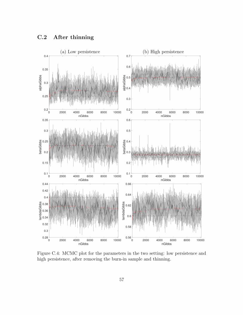
C.2 After thinning

(a) Low persistence (b) High persistence

0 2000 4000 6000 8000 10000

nGibbs

0.2

0.25

0.3

0.35

0.4

alp

haG

ibbs

0 2000 4000 6000 8000 10000

nGibbs

0.2

0.3

0.4

0.5

0.6

0.7

alp

haG

ibbs

0 2000 4000 6000 8000 10000

nGibbs

0.1

0.15

0.2

0.25

0.3

0.35

beta

Gib

bs

0 2000 4000 6000 8000 10000

nGibbs

0.1

0.2

0.3

0.4

0.5

0.6

beta

Gib

bs

0 2000 4000 6000 8000 10000

nGibbs

0.28

0.3

0.32

0.34

0.36

0.38

0.4

0.42

0.44

lam

bdaG

ibbs

0 2000 4000 6000 8000 10000

nGibbs

0.56

0.58

0.6

0.62

0.64

0.66

lam

bdaG

ibbs

Figure C.4: MCMC plot for the parameters in the two setting: low persistence andhigh persistence, after removing the burn-in sample and thinning.

57

(a) Low persistence (b) High persistence

Figure C.5: Histograms of the MCMC draws for the parameters in both settings: lowpersistence and high persistence, after removing the burn-in sample and thinning.

58

(a) Low persistence (b) High persistenceα α

-0.2

0

0.2

0.4

0.6

0.8

1

AC

F

0 5 10 15 20

Lag

-0.2

0

0.2

0.4

0.6

0.8

1

AC

F

0 5 10 15 20

Lag

β β

-0.2

0

0.2

0.4

0.6

0.8

1

AC

F

0 5 10 15 20

Lag

-0.2

0

0.2

0.4

0.6

0.8

1

AC

F

0 5 10 15 20

Lag

λ λ

-0.2

0

0.2

0.4

0.6

0.8

1

AC

F

0 5 10 15 20

Lag

-0.2

0

0.2

0.4

0.6

0.8

1

AC

F

0 5 10 15 20

Lag

Figure C.6: Autocorrelation function for the parameters in both low persistence andhigh persistence settings, after removing the burn-in sample and thinning.

59