arX

iv:0

712.

2259

v3 [

mat

h-ph

] 2

0 A

ug 2

008

Poisson-Lie T-Duality and non trivial

monodromies

A. Cabrera *, H. Montani† & M. Zuccalli*

* Departamento de Matematicas, Universidad de La Plata,Calle 50 esq. 115 (1900) La Plata, Argentina

† Centro Atomico Bariloche and Instituto Balseiro(8400) S. C. de Bariloche, Rıo Negro, Argentina

August 20, 2008

Abstract

We describe a general framework for studying duality among differentphase spaces which share the same symmetry group H. Solutions corre-sponding to collective dynamics become dual in the sense that they aregenerated by the same curve in H. Explicit examples of phase spaceswhich are dual with respect to a common non trivial coadjoint orbitOc,0 (α, 1) ⊂ h∗ are constructed on the cotangent bundles of the factors ofa double Lie group H = N ⋊⋉ N∗. In the case H = LD, the loop group ofa Drinfeld double Lie group D, a hamiltonian description of Poisson-LieT-duality for non trivial monodromies and its relation with non trivialcoadjoint orbits is obtained.

Contents

1 Introduction 2

2 Setting for duality and the diagram 4

3 Phase spaces on Lie groups, central extensions and double Liegroups. 83.1 Chiral WZNW type phase spaces . . . . . . . . . . . . . . . . . . 8

3.1.1 Symplectic equivalence between Oc,0 (α, 1) and Oc,−α (0, 1) 113.2 Double Lie groups and sigma model phase spaces . . . . . . . . . 12

3.2.1 Phase spaces on T ∗N . . . . . . . . . . . . . . . . . . . . . 133.2.2 Phase spaces on T ∗N∗ . . . . . . . . . . . . . . . . . . . . 16

1

4 Poisson Lie T -Duality 194.1 Dualizable subspaces . . . . . . . . . . . . . . . . . . . . . . . . . 204.2 The PL T -duality scheme . . . . . . . . . . . . . . . . . . . . . . 22

5 Associated hamiltonian Systems 245.1 Master WZNW-type model on (T ∗H, ωc,θ) . . . . . . . . . . . . . 245.2 Collective hamiltonian on the factor (N × n∗, ωo) . . . . . . . . . 26

5.2.1 Collective system for µ0,0 : N × n∗ −→ hc,0 . . . . . . . . 265.2.2 Collective system for µ0,α : N × n∗ −→ h∗c,−α . . . . . . . 27

5.3 Collective hamiltonian on the factor (N∗ × n, ωo) . . . . . . . . . 27

6 Loop groups and Poisson Lie T-duality for trivial monodromies 286.1 The chiral WZNW phase space . . . . . . . . . . . . . . . . . . . 306.2 A symplectic LD action on LG∗ × Lg . . . . . . . . . . . . . . . 326.3 T-duality diagram for non trivial monodromies . . . . . . . . . . 336.4 Induced hamiltonian systems on loops groups . . . . . . . . . . . 33

6.4.1 The induced lagrangians . . . . . . . . . . . . . . . . . . . 35

7 Conclusions 37

8 Appendix 1 37

9 Appendix 2 38

1 Introduction

Poisson-Lie T-duality [1] refers to a non-Abelian duality between two 1 + 1dimensional σ-models describing the motion of a string on targets which are adual pair of Poisson-Lie groups. The lagrangians of the models are written interms of the underlying bialgebra structure of the Lie groups, and Poisson-Lie T-duality stems from the self dual character the Drinfeld double. Indeed, classicalT-duality transformation relates some dualizable subspaces of the associatedphase spaces, mapping solutions reciprocally. Many different approaches haverevealed the canonical character of these transformations [1] [2] [4] [5] [6]. Thereare also WZNW-type models with target on the associated Drinfeld doublegroup D whose dynamics encodes in some way the equivalent sigma models onthe factors [1] [7].

In reference [8], most of the known facts of T-duality were embodied in apurely hamiltonian approach, offering a unified description of its classical as-pects based on the symplectic geometry of the underlying loop group phasespaces. There, PL T-duality is realized via momentum maps from the cotan-gent bundles of both the factor Lie groups to a pure central extension coadjointorbit of the Drinfeld double. These moment maps are associated to the dressingsymmetry inherited from the double Lie group structure. Since the hamilto-nians corresponding to the σ-models are in collective form, the pre-images ofcoadjoint orbits through the moment maps allows us to identify the dualizable

2

spaces that are preserved by the dynamics. On the other hand, this orbits aresymplectomorphic to the reduced phase space of one of the chiral sectors of theWZNW model with trivial monodromy, making clear the geometric content ofthe relation between the cotangent bundle of D and its factors. These facts areencoded in the commutative diagram

(Ld∗Γ; , KK)

(T ∗LG;ωo)

µ-

µ

(T ∗LG∗; ωo)

(ΩD;ωΩD)

Φ

6

- (1)

where the left and right vertices are the phases spaces of the σ-models, withthe canonical Poisson (symplectic) structures, Ld∗Γ is the dual of the centrallyextended Lie algebra of LD with the Kirillov-Kostant Poisson structure, andΩD is the symplectic manifold of based loops. In particular, µ and µ are derivedas momentum maps associated to hamiltonian actions of the centrally extendedloop group LDc,0 on the σ-model phase spaces. The subsets which can relatedby T-duality are the pre images under µ and µ of the coadjoint orbit O(0, 1) ≃ΩD where both momentum maps intersect and the dualizable subspaces areidentified as the orbits of ΩD, their symplectic foliation. From this setting, wewere able to build dual hamiltonian models by taking any suitable hamiltonianfunction on the loop algebra of the double and lifting it in a collective form [16].For particular choices, the lagrangian formalism is reconstructed obtaining theknown dual sigma and WZNW-like model models.

The present work is devoted to the extension of the framework developedin [8] in order to include T-duality based on non trivial coadjoint orbits of theform O(α, 1), leading to meaningful changes as a consequence of the non trivialmonodromies.

To that end, we describe a general setting for studying duality betweendifferent hamiltonian systems with phase spaces P and P linked by a commonhamiltonian H-action. This duality is supported on some coadjoint orbit O ⊂ h∗

where the corresponding momentum maps intersect cleanly. Thus, diagram (1)becomes a special case of this situation.

Motivated by the previous T-duality investigations, we work out examplesbuilt on the cotangent bundles of a double Lie group H = N ⋊⋉ N∗ and onits factors (N,N∗). As a corner stone of the T-duality scheme we choose a nontrivial coadjoint orbit O(α, 1) of the centrally extended group H, with α in eithern or n∗. This orbit, in turn, can be related to a coboundary shifted trivial one.We find out some actions of H on the cotangent bundles of the factors (N,N∗)whose associated equivariant momentum maps serve as the linking arrows withthe coadjoint orbits mentioned before. This gives the basic structure underlyingT-duality. Hence, collective dynamics completes the approach introducing theappropriate dynamics. However, we shall see that since the symmetric role

3

played by the factors in the case described by diagram (1) no longer holds,richer T-dual models emerge. Later, all these is applied in the case H = LDwith D = G ⋊⋉ G∗, driving in a constructive way to some previously studiedmodels.

This work is organized as follows: in Section 2, we describe a general settingfor studying duality based on a common hamiltonian G-action and give somesimple examples; in Section 3, we present the general geometric frameworklinking coadjoint orbits on H and the phase spaces on its factors (N,N∗). Therole played by central extensions is also analyzed, and the symmetry actionsleading to the relevant momentum maps are constructed. In Section 4.2, allthe kinematic aspects studied before are condensed into a new PL T-dualityscheme based on collective dynamics. The construction of the resulting H-hamiltonian systems and the associated lagrangians is addressed in Section 5.In Section 6, we illustrate the previous developments for H = LD, with D =G ⋊⋉ G∗, discussing some properties of the models. Finally, some conclusionsand comments are condensed in the last Section 7.

2 Setting for duality and the diagram

In this section, we generalize the geometrical framework behind T -duality whichwas described in [8].

Let us consider a Poisson manifold (P, , P ) on which a Lie group G acts bycanonical transformations. Suppose further that the action is hamiltonian withAd∗-equivariant moment map J : P −→ g∗, where g denotes the Lie algebraof G. Recall that J : P −→ g∗ is a Poisson map for the (+) Kirillov-KostantPoisson bracket , KK on g∗. Following [16], we define

Definition: We say that the G-hamiltonian system (P, , P , G, J,H), withHamilton function H : P −→ R, has dynamics of collective motion typeif H is given by the composition

H = h Jwith h : g∗ −→ R.

For this kind of systems, the dynamics is confined in a coadjoint orbit, as itis stated in the next theorem.

Theorem: Let (P, , P , G, J, hJ) be a collective G-hamiltonian system. Thenfor the initial value p0 ∈ P s.t. J(p0) = J0 ∈ g∗ the solution p(t) of theHamilton equations of motion in P is given by

p(t) = g(t) · p0

with g(t) ∈ G such that

gg−1 = dhξ(t)

g(0) = e

4

where ξ(t) ∈ g∗ is the solution of the Hamilton equations on g∗

ξ(t) = −ad∗dhξ(t)ξ(t)

ξ(0) = J0.

The above result can be summarized in the following diagram

(P, , P , h J) (T ∗G,ωo, h s)

(g∗, , KK , h)

s

?J

-

(2)

where s(αg) = R∗gαg for αg ∈ T ∗

gG is the momentum map associated to thelifting to T ∗G of the left action Lg of G on itself and Rg denotes the righttranslation in G. The map s is a Poisson map in relation with the Kirillov-Kostant Poisson bracket on g∗ defined as F,HKK (η) = + 〈η, [dF, dH ]〉.Remark: (Groupoid actions) In fact, T ∗G g∗ is a symplectic groupoid inte-

grating the Poisson manifold (g∗, , KK) ([9]) and any such diagram asabove with complete Poisson J , defines a T ∗G-groupoid action on P . Inthis case, it coincides with a usual G-action. As in the above proposition,solutions in P for collective H are given by this groupoid action αg(t) · p0

with αg(t) a solution to the corresponding collective hamiltonian eqs. on(T ∗G,ω0, h s).

Notice that, if (P , , P , G, J , h J) is another collective hamiltonian G-system, we would have the analogous diagram to (2) so we can glue both ofthem yielding

(P, , P , h J) (T ∗G,ω0, h s) (P , , P , h J)

J - J

(g∗, , KK , h)

s

?

(3)

If both systems share some non empty set in the images of the correspondingmomentum maps, then part of its dynamics can be described in a unified way,as stated in the next proposition.

Proposition: Let (P, , P , G, J, h J) and (P , , P , G, J , h J) be collective

G−hamiltonian systems such that ImJ ∩ ImJ 6= ∅. Then, for J0 ∈ImJ ∩ ImJ ⊂ g∗ and p0 ∈ J−1(J0), p0 ∈ J−1(J0), the solutions p(t) andp(t) corresponding to the initial values p0, p0 for the hamiltonian equationson (P, , P , h J) and (P , , P , h J), respectively, are given by

p(t) = g(t) · p0,

p(t) = g(t) · p0

5

where g(t) ∈ G is the curve solution to

gg−1 = dhξ(t) (4)

g(0) = e

with ξ(t) ∈ g∗ the solution of the hamiltonian equations on g∗

ξ = −ad∗dhξ(t)ξ(t)

ξ(0) = J0.

Thus both solutions on P and P , with compatible initial conditions, areobtained from the same curve g(t) in G. So, if we had one of them (say p(t))we can map it through J to g∗ and then, by solving eq. (4), obtain the othersolution p(t) = g(t) · p0. Motivated by field theory applications we do thefollowing definition:

Definition: Two collective G-hamiltonian systems (P, , P , G, J, h J) and(P , , P , G, J , h J) with the same collective function h and such that

there exist a subspace O ⊂ ImJ ∩ ImJ , are said to be dual to each otherwith respect to O.

When ImJ ∩ ImJ = ∅, then duality is trivial. In general, ImJ ∩ ImJ is adisjoint union of coadjoint orbits in g∗.

Remark: (Transitivity) Note that being dual with respect to a certain fixedsubspace O ⊂ g∗ is a transitive property.

In the following sections, we shall apply this setting to systems coming fromclassical field theory. Meanwhile, we show some applications in simple examples.

Example: (Rigid body dual to a Pendulum) This example comes from[18]. The hamiltonian system (T ∗SE(2), ω0, h J) describes the motionof a rigid body where ω0 denotes the standard symplectic structure onT ∗SE(2) and J the moment map corresponding to the lifted left SE(2)action. The collective function h : se(2)∗ −→ R is

h(β) =1

2〈β,Nβ〉

for N : se(2)∗ ≃ R3 −→ R

3 given by the matrix

N =

0 0 0

0 c(

1I1

− 1I2

)0

0 0 1

where c =(

1I1

− 1I3

)−1

and I1 < I2 < I3 are the principal moments of

inertia of the underlying rigid body. Now, consider the hamiltonian system

6

(T ∗S1, ω, h J) where ω denotes (k1k2) times the standard symplecticstructure on T ∗S1, with the momentum map J : T ∗S1 −→ se(2)∗ being

J(θ, p) = (r sinθ, r cosθ, k1k2 p)

Here

1

k21

=1

I1− 1

I3,

1

k22

=1

I2− 1

I3,

1

k23

= c

(1

I1− 1

I2

)

and r =√

2K denotes the constant value of the function

K(β) =1

2

(1

I1− 1

I3

)β2

1 +1

2

(1

I2− 1

I3

)β2

2 .

From the dual Hamilton equations on T ∗S1, one easily arrives to thefollowing equation for θ(t)

d2

dt2θ = −K

(1

I1− 1

I2

)sin(2θ)

which is the equation for the motion of a pendulum with angle θ. Itthus follows from the above considerations that the rigid body hamilto-nian system is dual to a pendulum hamiltonian system with respect toO := ImJ ⊂ se(2)∗.

Example:(Coadjoint orbits) Generalizing the previous example, supposethat (P, , P , G, J, hJ) is a G-hamiltonian system such that the coadjointorbit Oµ ⊂ ImJ . Then the following diagram

(P, , P , h J) (Oµ, ωKKµ , h i)

(g∗, , KK , h) iJ -

says that (P, , P , hJ) is dual to (Oµ, ωµ, h i) with respect to Oµ ⊂ g∗,where i : Oµ → g∗ denotes the inclusion and ωKKµ the Kirillov-Kostantsymplectic structure on the coadjoint orbit Oµ corresponding to , KK ing∗.

Example: (Dual groups) Suppose that (H,N,N∗) are a triple of Lie groupsfor which H is the corresponding perfect Drinfeld double of the Poisson-Liegroups N and N∗ [13]. Moreover, suppose that there is a one cocycle

C : H −→ h∗

i.e. a map satisfying

C (lk) = AdH∗l−1C (k) + C (l) , l, k ∈ H

7

with the additional property C(N ⊆ H) ⊆ n := n-annihilator in h∗ andC(N∗ ⊆ H) ⊆ n∗ := n∗-annihilator in h∗. Then, we can consider thefollowing diagram corresponding to (3)

(T ∗N,ωo, h J) (T ∗H,ωC , h s) (T ∗N∗, ωo, h J)

J - J

(h∗, , C, h)

s

?

The maps involved are J(g, α) = C(g) + AdH∗g α and J(g, X) = C(g) +

AdH∗g X . The structures are: ωC the right invariant C-modified symplectic

structure [12], , C the affine Poisson structure on h∗ defined by C. Withthese, s(d, ξ) = ξ is the (source) Poisson map. Notice that the orbit of theC-affine coadjoint action on h∗ through 0 is C(H) ⊂ h∗ (see below) andgives the intersection ImJ∩ImJ . So, (T ∗N, ωo, hJ) and (T ∗N∗, ωo, hJ)are duals to each other (and, hence, also to (T ∗H, ωC , h s)) with respectto O := C(H). See also [8].

3 Phase spaces on Lie groups, central extensions

and double Lie groups.

In this section, we elaborate on the structure proposed in the previous section(the last example above) for describing duality on non-trivial coadjoint orbits.Dual phase spaces are built from the factors N and N∗ of a (perfect) double Liegroup H = N ⋊⋉ N∗, and the corresponding H-action on them is constructed bymeans a certain Lie algebra h-cocycle. In contrast with ref. [8], the symmetricrole that the factors N and N∗ played in the duality formulation is broken byconsidering solutions associated to an element1 α ∈ n∗.

3.1 Chiral WZNW type phase spaces

Let us begin recalling some results of [12] with explicit considerations for cobound-ary modified cocycles. Let H be a Lie group and T ∗H ∼ H × h∗ its cotan-gent bundle trivialized by left translations. We consider on it the canonical1-form ϑo and the symplectic form ωo = −dϑo, which on vectors (v, ξ), (w, λ) ∈T(l,η) (H × h∗) = TlH × h∗ is

〈ωo, (v, ξ) ⊗ (w, λ)〉(l,η) = −〈ξ, l−1w〉 + 〈λ, l−1v〉 + 〈η, [l−1v, l−1w]〉 (5)

A new symplectic structure can be obtained by adding a two cocycle c :h ⊗ h −→ R, derived from an Ad∗-cocycle C : H −→ h∗, characterized byc (AdgX, AdgY) = c (X,Y) +

⟨C(g−1

), [X,Y]

⟩for all X,Y ∈ h. Also recall

1The case studied in [8] corresponds to the α = 0, i.e., trivial monodromy solutions case.

8

that C (lk) = AdH∗l−1C (k)+C (l) and c ≡ − dC|e : h −→ h∗ produces c (X,Y) ≡

〈c (X) ,Y〉. In the remaining, we fix C and consider its shifting by a coboundaryBθ defined by θ ∈ h∗ as

Bθ (l) = Ad∗l−1θ − θ

defining the following shifted cocycle Cθ and two cocycle cθ,

Cθ (l) = C (l) −AdH∗l−1θ + θ

cθ (X,Y) = c (X,Y) − 〈θ, [X,Y]〉 .

The extended symplectic form ωc,θ on T ∗H, for (v, ξ), (w, λ) ∈ T(l,η) (H × h∗) =TlH × h∗ is given by

〈ωc,θ, (v, ξ) ⊗ (w, λ)〉(l,η) = 〈ωo, (v, ξ) ⊗ (w, λ)〉(l,η) − cθ(vl−1 ,wl−1

)(6)

which is invariant under right translations of H. This symplectic manifold(H × h∗, ωc,θ) is related to the phase space of chiral modes of the WZNW modelswhen loops groups are considered.

Now, consider the extended coadjoint action AdH∗

θ; of the corresponding cen-trally extended group Hc,θ on h∗c,θ, the dual of the central extended Lie algebrahc,θ of h by the cocycle cθ. It is given by

AdH∗

θ;l−1 (ξ, b) = (Ad∗l−1ξ + bCθ (l) , b)

and the linear Poisson bracket ,c,θ on h∗c,θ by

〈X,−〉 , 〈Y,−〉c,θ (ξ, 1) =⟨ξ, [X,Y]h

⟩− cθ (X,Y)

for X,Y ∈ h. Its symplectic leaves are the AdH∗

θ; −coadjoint orbits equippedwith the Kirillov-Kostant symplectic structure.

The AdH∗

θ; -equivariant momentum map JRc,θ : H × h∗ → h∗c,θ associated tothe induced symplectic Hc,θ-action on (H × h∗, ωc,θ) is

JRc,θ (l, η) = (η −Ad∗lCθ (l) , 1) (7)

Remark (Affine coadjoint action) We observe that everything that follows canbe carried out by means of the affine coadjoint action of the group H,withoutextension, on h∗

AdH∗

Aff ;l−1ξ = Ad∗l−1ξ + Cθ (l)

instead of the extended one AdH∗

θ; of Hc,θ on h∗c,θ. This affine action gives

rise to the coadjoint affine orbits OAffα and the corresponding affine Pois-

son bracket on h∗, without further reference to central extensions. How-ever, we keep the central extension framework for simplicity.

9

The phase spaces (H × h∗, ωc,θ) play a central role in our T -duality scheme:most of its features rely on their symmetry properties and the correspondingreduced spaces are the bridge connecting T -dual systems. So let us work out acouple of related phase spaces which we shall be concerned with.

S1- For θ = 0, the Marsden-Weinstein [10] reduction procedure can be ap-plied to a regular value of the form (α, 1) ∈ h∗c,0 within the phase space

(H × h∗, ωc,0). We get that[JRc,0

]−1

(α, 1) ≃ H is a presymplectic manifold

with the restricted 2-form

ω−α (v,w) := ωc,0|[JRc,0]

−1(α,1)

(v,w) = c−α(l−1v, l−1w

)(8)

for v,w ∈TlH. Its null distribution is spanned by the infinitesimal gener-ators of the action of the subgroup Hα := kerC−α, so that the reducedsymplectic space is

M(α,1)c,0 :=

[JRc,0

]−1

(α, 1)

Hα≃ H

Hα

where the right action of Hα on H is considered. Denoting the fiber bundle

HΠH/Hα−→ H/Hα, then the base H/Hα is endowed with a symplectic form ωR

defined by Π∗H/Hα

ωR = ω−α. This form is invariant under the residual left

action of H on H/Hα and has associated momentum map Φc,0 : H/Hα −→h∗c,0

Φc,0 : H/Hα −→ h∗c,0 / Φc,0 (l · Hα) = (C−α (l) + α, 1)

which is AdH∗

θ=0-equivariant and gives a local symplectic diffeomorphism

from (H/Hα, ωR) to the coadjoint orbit Oc,0 (α, 1) equipped with theKirillov-Kostant symplectic structure ωKKc,0 . Notice that the subgroup Hα

coincides a with the stabilizer subgroup [Hc,0](α,1) of the point (0, 1) ∈h∗c,−α.

S2- For arbitrary θ = −α ∈h∗, the reduction procedure can be applied to the

regular value (0, 1) ∈ h∗c,−α of ImJRc,−α. The level set[JRc,−α

]−1

(0, 1) ∼= H

is again a presymplectic manifold with restricted 2-form

ω−α (v,w) := ωc,−α|[JRc,−α]

−1(0,1)

(v,w) = c−α(l−1v, l−1w

)(9)

for v,w ∈TlH. The null distribution of ω−α is spanned by the infinitesimalgenerators of the (right) action of the subgroup Hα. Hence, the reducedsymplectic space is

M(0,1)c,−α :=

[JRc,−α

]−1

(0, 1)

Hα

∼= H

Hα

10

again. The symplectic form ωR is defined by Π∗H/H−α

ωR = ω−α as before.Recall that ωR is invariant under the residual left action and that the as-

sociated AdH∗

−α-equivariant momentum map Φc,−α : H/Hα −→ h∗c,−α nowreads

Φc,−α (l · Hα) = (C−α (l) , 1) (10)

Moreover, Φc,−α is a local symplectic diffeomorphism onto the coadjointorbit Oc,−α (0, 1) ⊂ h∗c,−α equipped with the Kirillov-Kostant symplec-

tic structure ωKKc,−α. Notice that the subgroup Hα coincides a with thestabilizer subgroup [Hc,−α](0,1) of the point (0, 1) ∈ h∗c,−α.

3.1.1 Symplectic equivalence between Oc,0 (α, 1) and Oc,−α (0, 1)

The above described reduced spaces can be linked through the shifting trickas follows. The orbits Oc,0 (α, 1) ⊂ h∗c,0 and Oc,−α (0, 1) ⊂ h∗c,−α are bothisomorphic to H/Hα as symplectic manifolds and, moreover,

Proposition: The map ϕ : h∗c,−α −→ h∗c,0

ϕ (η, 1) = (η + α, 1) (11)

is a Poisson diffeomorphism. When restricted to ϕ : Oc,−α (0, 1) ⊂ h∗c,−α−→ Oc,0 (α, 1) ⊂ h∗c,0 it becomes a symplectic diffeomorphism.

Proof: The underlying vector space of h∗c,−α, h∗c,0 is the same h∗ ⊕ R.Introducing the Legendre transform Lf : h∗ ⊕ R −→ h of some function f ∈C∞

(h∗c,β

)as

〈Lf (η, 1) , ξ〉 =d

dtf (η+tξ, 1)

∣∣∣∣t=0

The Poisson structures on the generic h∗c,β is

f, hc,β (η, 1) = 〈η − β, [Lf (η, 1) ,Lh (η, 1)]〉 + c (Lf (η, 1) ,Lh (η, 1))

Then, from this expression and having in mind that Lf (ϕ (η, 1)) = Lfϕ (η, 1),it is immediate to see that

f, hc,0 (ϕ (η, 1)) = f ϕ, h ϕc,−α (η, 1) .

Thus the hamiltonian vector fields associated to the the functions f ∈ C∞(h∗c,0)

and f ϕ ∈ C∞(h∗c,−α

)are ϕ-related

ϕ∗

[adc,−α∗

(Lfϕ(η,1),1) (η, 1)]

= adc,0∗

(Lf(η+α,1),1) (η + α, 1)

The orbits Oc,−α (0, 1) ⊂ h∗c,−α and Oc,0 (α, 1) ⊂ h∗c,0 are

Oc,−α (0, 1) =(C−α

(l−1), 1)/l ∈ H

=

H

Hc,−α(0,1)

Oc,0 (α, 1) =(C(l−1)

+Ad∗l α, 1)/l ∈ H

=

H

Hc,0(α,1)

11

where Hc,−α(0,1) = Hc,0

(α,1) = Hα ≡ kerC−α are the stabilizer subgroups of (0, 1) ∈h∗c,−α and (α, 1) ∈ h∗c,0. The restriction of the above Poisson structures tothese orbits endow them with the corresponding Kirillov-Kostant symplecticforms ωKKc,−α, ω

KKc,0 , and the diffeomorphism ϕ : Oc,−α (0, 1) −→ Oc,0 (α, 1),

ϕ(C−α

(l−1))

= C−α

(l−1)

+ α, becomes a symplectic one. In fact, for η =

C−α

(l−1)

and after a direct computation, one recovers

⟨ωKKc,0 , ad

c,0∗

(Lf(η+α,1),1) (η + α, 1) ⊗ adc,0∗

(Lf(η+α,1),1) (η + α, 1)⟩

(η+α,1)

=⟨ωKKc,−α, ad

c,−α∗

(Lfϕ(η,1),1) (η, 1) ⊗ adc,−α∗

(Lhϕ(η,1),1) (η, 1)⟩

(η,1)

showing that ϕ∗ωKKc,0 = ωKKc,−α.Hence, all the above maps can be resumed in the following diagram

(M

(α,1)c,0 , ω−α

)-(H

Hα, ωR

)

(M

(0,1)c,−α, ω−α

)

? ?

-

(Oc,0 (α, 1) , ωKKc,0

) ϕ

(Oc,−α (0, 1) , ωKKc,−α

)

(12)

where all the arrows are symplectic isomorphisms. This result shall be used fordescribing a WZNW-type model on a double Lie group H as described in thenext section.

3.2 Double Lie groups and sigma model phase spaces

We assume now that H is a Drinfeld double Lie group [13, 14], H = N ⋊⋉ N∗

with tangent Lie bialgebra h = n ⊕ n∗. This bialgebra h is naturally equippedwith the non degenerate symmetric Ad-invariant bilinear form (, )h provided bythe pairing between n and n∗ and which turns them into isotropic subspaces.Let ψ denote the identification between h and h∗ induced by this bilinear form(, )h. For the sake of brevity, we often omit it from formulas when there is nodanger of confusion.

The aim of the following subsections is to construct dual phase spaces fromthe factors N and N∗ as described in section 2. T-duality over the trivial orbitOc,0(0, 1) was considered in ref. [8] in relation to Poisson-Lie T-duality for loopgroups and trivial monodromies. Now, we focus our attention into exploringhamiltonian H-actions on phase spaces T ∗N and T ∗N∗ such that they becomeT-dual over a non-trivial coadjoint orbit Oc,0(α, 1), with α in n or n∗. Noticethat, once α is chosen in one of the factors, the symmetric role played by Nand N∗ in the construction is broken. By the Poisson isomorphism (11), equiv-alent systems will be constructed on the orbit Oc,−α(0, 1), for α in n or n∗.

12

Hence, we can choose the momentum maps for associated H-actions to be val-

ued on(h∗c,0, , c,0

)or(h∗c,−α, , c,−α

). Poisson-Lie T-duality for non-trivial

monodromies in the loop group case is described in section 6.On double Lie groups there exist reciprocal actions between the factors N

and N∗ named dressing actions [15],[14]. Since every element l ∈ H can bewritten as l = gh, with g ∈ N and h ∈ N∗, the product hg in H can be expressed

as hg = ghhg, with gh ∈ N and hg ∈ N∗. The dressing action of N∗ on N isthen defined as

Dr : N∗ × N −→ N | Dr

(h, g)

= ΠN

(hg)

= gh

where ΠN : H −→ N is the projector. For ξ ∈ n∗, the infinitesimal generator ofthis action at g ∈ N is

ξ −→ dr (ξ)g = − d

dtDr(etξ, g

)∣∣∣∣t=0

such that, for η ∈ n∗, we have[dr (ξ)g , dr (η)g

]= dr ([ξ, η]n∗)g. It satisfies the

relation AdHg−1ξ = −g−1

dr (ξ)g + Ad∗gξ, where AdHg−1 ∈ Aut (h) is the adjoint

action of H on its Lie algebra. Then, using the projector Πn : h −→ n, we canwrite dr (ξ)g = −g ΠnAd

Hg−1ξ.

Let us now consider the action of H on itself by left translations Labgh =

abgh. Its projection on the one of the factors, N for instance, yields also anaction of H on that factor

ΠN

(Labgh

)= ΠN

(abgh

)= agb

The projection on the factor N∗ is obtained by the reversed factorization of H,namely N∗ × N, such that

ΠN∗

(Lbahg

)= ΠN∗

(bahg

)= bha

In the next subsections, we lift these actions to T ∗N and T ∗N∗ and twistthem using a cocycle. The resulting ones play a central role in constructing T -dual phase spaces out of these cotangent bundles, turning them in hamiltonianspaces for different central extensions of the group H.

3.2.1 Phase spaces on T ∗N

Hamiltonian Hc,0-spaces We now consider a phase space T ∗N ∼= N × n∗,trivialized by left translations and equipped with the canonical symplectic formωo. We shall realize the symmetry described above, as it was introduced in [8].

We promote this symmetry on T ∗N to a centrally extended one by means ofan n∗-valued cocycle CN∗

: N∗ −→ n∗,

dN×n∗

0 : Hc,0 × (N × n∗) −→ (N × n∗)

dN×n∗

0

(ab, (g, λ)

)=

(agb, AdH∗

(bg)−1λ+ CN∗

(bg)) (13)

13

Aiming to repeat the same construction on a dual phase space, the adjoint N-cocycle CN∗

: N∗ −→ n∗ is assumed to be the restriction to the factor N of anH-coadjoint cocycle on C : H −→ h∗, namely CN∗

:= CH|N∗ , in such a way that

C|N : N −→ n

C|N∗ : N∗ −→ n∗ (14)

We shall say that, in this case, C is compatible with the factor decomposition.One of the key ingredients for describing the resulting duality is that the aboveH-action is hamiltonian.

Proposition: Let T ∗N be identified with N × n∗ via left translations and en-dowed with its canonical symplectic structure. The action d

N×n∗

0 , definedin eq.(13) from a cocycle C compatible with the factor decomposition, ishamiltonian and the momentum map µ0,0 : (N × n∗, ωo) →

(h∗c,0, , c,0

)

µ0,0 (g, λ) = AdH∗

0;g−1 (ψ (λ) , 1) =(ψ(AdH

g λ+ CN∗

(g)), 1).

is AdH∗

0; -equivariant.

Proof : The infinitesimal generator of the action (13) associated to (X, ξ) ∈h is the vector field

(X, ξ)N×n∗

∣∣(g,λ)

=(Xg − dr (ξ)g ,

[Ad∗gξ,λ

]− c

(Ad∗gξ

))

By an straightforward calculation one may see that

ı(X,ξ)N×n∗ωo

∣∣∣(g,λ)

= d〈AdH∗g−1λ+ C (g) , (X,ξ) 〉

so that f(X,ξ) (g, λ) ≡ 〈AdH∗g−1λ + C (g) , (X,ξ) 〉 is the hamiltonian function as-

sociated to the vector field (X, ξ)N×n∗ . Then, µ0,0 : N × n∗ −→ h∗c,0 definedas

µ0,0(g, λ) =(ψ(AdH∗

g−1λ+ C (g)), 1)

is the momentum map associated to the action (13).

Hence, since (X, ξ)N×n∗ is hamiltonian for all ((X, ξ) , s) ∈ hc,0, and dN×n∗

0

leaves the canonical symplectic form invariant. Furthermore, µ0,0 is Ad -equivariant

µ0,0

(dN×n∗

0

(ab, (g, λ)

))= µ0,0

(agb, AdH∗

(bg)−1λ+ CN∗

(bg))

=

(AdH∗

(abg)−1λ+ CN∗

(abg), 1

)

then

µ0,0

(dN×n∗

0

(ab, (g, λ)

))= Ad

H∗

0;(ab)−1µ0,0 (g, λ)

as required.As stated in the introduction, for constructing dualizable subspaces, we need

to fix an α ∈ n∗ and study the µ0,0-pre image of the orbit Oc,0 (α, 1) ⊂ h∗c,0.

14

Hamiltonian Hc,−α-spaces In view of the equivalence stated in section 3.1.1,we can think of T ∗N ≃ N×n∗ as phase space linked by a momentum map valuedon h∗c,−α. This is attained by considering the coboundary shifted cocycle

CN∗

−α

(h)

= CN∗

(h)

+Adhα− α

for some α ∈ n∗, thus enabling to introduce an Hc,−α-action on T ∗N ≃ N × n∗

defined as

dN×n∗

α : Hc,−α× (N × n∗) −→ (N × n∗)

(15)

dN×n∗

α

(ab, (g, η)

)=(agb, Adbgη + CN∗

−α

(bg))

for ab ∈ H = N ⋊⋉ N∗ and (g, η) ∈ T ∗N. It is worth to remark this action isnot a cotangent lift of a transformation on N, and that it is meaningful just forα ∈ n∗, it does not make sense to for arbitrary α ∈ h∗.

The shifted H−cocycle

C−α (l) = C (l) +AdH∗l−1α− α (16)

does not satisfy property (14), so the above action may be not hamiltonian in(N × n∗, ωo) (compare to example 2) unless some constraint is imposed on α.

Proposition: Let α ∈ n∗ then, provided the condition

Πn∗ [X,α] = 0 (17)

is fulfilled for all X ∈ n, then the above defined shifted H-cocycle C−α

becomes compatible with the factor decomposition H = N ⋊⋉ N∗. Conse-quently, in this case, the action d

N×n∗

α : Hc,−α×(N × n∗, ωo) −→ (N × n∗, ωo)

defined by (15) is hamiltonian. The associated AdH∗

α; -equivariant momen-

tum map µ0,α : (N × n∗, ω0) −→(h∗c,−α, , c,−α

)is given by

µ0,α (g, η) = AdH∗

α;g−1 (ψ (η) , 1) =(ψ(AdH

g η + C−α (g)), 1)

(18)

Alternatively, a hamiltonian Hc,−α-space on N × n∗ can be retrieved byconsidering a coboundary shifted symplectic form ωα on T ∗N ∼= N×n∗, obtainedby adding the coboundary bα (X,Y ) = 〈α, [X,Y ]n〉 to the canonical one so that,in body coordinates, it is

〈ωα, (v, ρ) ⊗ (w, ξ)〉(g,η) = −〈ρ, g−1w〉 + 〈ξ, g−1v〉 + 〈η + α, [g−1v, g−1w]〉for (v, ρ), (w, λ) ∈ T(g,µ) (N × n∗) = T ∗

gN × n.

Proposition: The action dN×n∗

α : Hc,−α × (N × n∗, ωα) −→ (N × n∗, ωα) de-

fined by (15) for α ∈ n∗, is hamiltonian. It has the associated AdH∗

α; -

equivariant momentum map µα,α : (N × n∗, ωα) −→(h∗c,−α, , c,−α

)

µα,α (g, η) = AdH∗

α;g−1 (ψ (η) , 1) =(ψ(AdH

g η + C−α (g)), 1)

(19)

15

Within this formulation, for constructing dualizable subspaces, we must lookat the µ0,α-pre-image of the orbit Oc,−α (0, 1) ⊂ h∗c,−α.

3.2.2 Phase spaces on T ∗N∗

Hamiltonian Hc,0-spaces In searching for some T -dual partners for the phasespaces on N×n∗ built above, we shall consider the symplectic manifold (N∗ × n, ωo)where ωo is the canonical 2-form in body coordinates. However, the way is notso direct as in the pure central extension orbit case [8] and a different strategyis needed in order to complete the diagram.

Let us consider H with the opposite factorization, denoted as H → H⊤ =N∗ ⊲⊳ N, so that every element is now written as hg with h ∈ N∗ and g ∈ N.

From 3.2, we get the action bG∗

: H × N∗ −→ N∗ defined as bG(ba, h

)= bha

with a ∈ N and h, b ∈ N∗.As we shall see below, the search for a hamiltonian H-action on N∗ × n will

leads us to meet again the restriction (17) on α. First, let us consider the arrow

z : (N∗ × n, ωo) −→ (h, , Aff ) ⊂ (hc,0, , c,0) ,

for α ∈ n∗, defined by the diagram

(H × h, ωRc ) iα(N∗ × n, ωo)

z

(h, , Aff)

s

?

whereiα(h, X) = (h, C(h) +AdH

h(X + α))

and the map s beings(l,X) = X

In the above diagram, H × h∗ is regarded as the trivialization of T ∗H byright translations equipped with the symplectic structure ωRc = ωRo − c R

〈ωRc , (v, Y ) ⊗ (w,Z)〉(h,X) = ωRo − c(vh−1 , wh−1

)

and ωRo denotes the standard symplectic structure on T ∗H in space coordinates.Recall that h ≃ h∗ is equipped with a non degenerate symmetric bilinear form(, )h : h⊗h −→ h. Finally, we recall the affine Poisson bracket , Affc,0 : C∞ (h)⊗C∞ (h) −→ C∞ (h)

(X,−)h , (Y,−)hAffc,0 (Z) = − ([X,Y],Z)h − c(X,Y) (20)

with X,Y,Z ∈ h, so that (h, , Aff) ⊂ (hc,0, , c,0) via X 7−→ (X, 1).

16

Remark (Affine coadjoint action) Via the isomorphism h ≃ h∗ induced by thebilinear form on h, we can work on (h, , Aff) by considering the affinecoadjoint action

AdHCθ ;lY = AdH

l Y + Cθ(l)

on h instead of the full extended coadjoint action AdH∗

θ; on h∗c,θ.

It is not hard to see that the map iα : (N∗ × n, ωo) −→ (H∗ × h, ωRc ) issymplectic, i.e., i∗αω

Rc = ωo for all α ∈ n∗, and that the map s : (H∗×h, ωRc ) −→

(h, , Aff) is a Poisson map.Thus, the resulting map z : (N∗ × n, ωo) −→ (h, , Aff) is a suitable candi-

date to be the generator of a hamiltonian action of H on the phase space N∗×n

and, moreover, its image z(N∗×n) contains the orbit Oc,0 (α, 1) ⊂ h∗ as desired.Notice that, if µ0,α : (N∗ × n, ωo) −→ (hc,−α, , c,−α) denotes the dual versionof the map (18), then the map z coincides with the composition ϕ µ0,α, wherethe isomorphism ϕ was given in (11). However, this candidate to momentummap fails to be a Poisson map for general α. This issue is addressed in thefollowing proposition.

Proposition: Let us define the map µϕ0,α : (N∗ × n, ωo) −→ (h, , Aff) as

µϕ0,α(h, X) := z = AdHhX + C−α

(h)

+ α = AdHh

(X + α) + C(h)

(21)

Then, it is Poisson iff condition (17) is satisfied:

Πn∗ [α,X ] = 0

∀X ∈ n. Here ωo is the canonical 2-form on N∗ × n trivialized by lefttranslations.

Proof: Let us sketch the guiding lines of this proof. It must be proved, forF ,G ∈ C∞ (h∗), that

F µϕ0,α,G µϕ0,α

N∗×n

(h, X

)= F ,GAff

(µϕ0,α

(h, X

))

The Poisson bracket , N∗×n is the symplectic one corresponding to ωo:

F µϕ0,α,G µϕ0,α

N∗×n

(h, X

)=⟨d(G µϕ0,α

), VFµϕ

0,α

⟩

where the hamiltonian vector field is Vf =(hδf, ad∗δfX − hdf

)and df = df +

δf ∈ n∗ ⊕ n, for f ∈ C∞ (N∗ × n). The explicit expression for the differentialsis

d(F µϕ0,α

)= h−1Πnad

hXAd

H∗

hdF + h−1Πnc−α

(AdH∗

hdF)

δ(F µϕ0,α

)= Πn∗AdH∗

hdF

17

that leads toF µϕ0,α,G µϕ0,α

N∗×n

(h, X

)

=⟨Πnad

hXAd

H∗

hdG + Πnc

(AdH∗

hdG),Πn∗AdH∗

hdF⟩

+⟨Πn

[Πn∗AdH∗

hdG, α

]+ Πn

[ΠnAd

H∗

hdG, α

],Πn∗AdH∗

hdF⟩

+⟨Πn∗AdH∗

hdG,−ad∗

Πn∗AdH∗

hdFX − Πnad

hXAd

H∗

hdF − Πnc

(AdH∗

hdF)⟩

−⟨Πn∗AdH∗

hdG,Πn

[Πn∗AdH∗

hdF , α

]− Πn

[ΠnAd

H∗

hdF , α

]⟩

If c is defined as in eq. (5) the restrictions c|n : n → n and c|n∗ : n∗ → n∗ are as-

sumed to be endomorphism of vector spaces. Then we write Πn∗ c(AdH∗

hdG)

=

c(Πn∗AdH∗

hdG)

and Πn∗c(AdH∗

hdF)

= c(Πn∗AdH∗

hdF). Besides these, we use

also the relations⟨

Πn∗adh

AdH∗

hdGX,ΠnAd

H∗

hdF⟩

=⟨ad∗X Πn∗AdH∗

hdG,ΠnAd

H∗

hdF⟩

⟨ΠnAd

H∗

hdG,Πn∗adh

AdH∗

hdFX

⟩=⟨ΠnAd

H∗

hdG, ad∗X Πn∗AdH∗

hdF⟩

and the Lie bracket in the double Lie algebra

[(X, η) , (Z, ξ)]h =([X,Z]n − ad∗ηZ + ad∗ξX, [η, ξ]n∗ − ad∗Xξ + ad∗Zη

)

for (X, η) , (Z, ξ) ∈ h. After a tedious but straightforward calculations, onearrives to

F µϕ0,α,G µϕ0,α

N∗×n

(h, X

)− F ,GAff

(µϕ0,α

(h, X

))

=⟨ΠnAd

H∗

hdG,Πn∗

[AdH∗

hdF , α

]⟩+⟨Πn

[AdH∗

hdG, α

],Πn∗AdH∗

hdF⟩

implying that µϕ0,α is a Poisson map provided the right hand side vanish forarbitrary dG, dF ∈ h. After some manipulations, it reduces to

⟨Ad∗

hΠndG,Πn∗

[Ad∗

hΠndF , α

]⟩= 0

that is equivalent to require that

Πn∗ [α,X ] = 0

for all X ∈ n.

Example: (Lu-Weinstein doubles [14]) When N∗ = K a compact simple realLie group, e.g. SU(N), then H = AN ×K where N = AN and N∗ = Kare the subgroups given by the Iwasawa decomposition of H = KC. Forany element α ∈ t, with t ⊂ n∗ being the Cartan subalgebra of k = Lie(K),condition (17) is satisfied (see Appendix 1).

18

For α fulfilling condition (17), an H-hamiltonian action on (N∗ × n, ωo) isobtained as stated below.

Proposition: Consider the symplectic manifold (N∗ × n, ωo) where ωo is thecanonical 2-form in body coordinates. The map b : Hc,0 × (N∗ × n) −→(N × n∗) defined as

b

(ba,(h, X

))=(bha, Ad

HahX + C−α

(ah))

(22)

is a hamiltonian H-action and µϕ0,α is the associated AdH∗

0; -equivariant themomentum map.

Remark That b as defined above is an action on N∗ × n follows from the factthat, when (17) is satisfied, then Πn∗C−α

(ah)

= 0. Thus, the expression

AdHahX + C−α

(ah)

is always n-valued as it should be.

Consequently, we have obtained the desired third hamiltonian H-space, namely(N∗ × n, ωo) ≡ (T ∗N∗, ωo), completing the diagram

T ∗N H/Hα T ∗N∗

Oc,0(α, 1) →(hc,0, , c,0)

Φc,0

?µϕ0,α

µ0,0 -

(23)

Hamiltonian Hc,−α-spaces Again, the equivalence stated in section 3.1.1enables to seek for a similar system now hanging on Oc,−α (0, 1) ⊂ h∗c,−α. In

doing so, we consider the map µα : (N∗ × n, ωo) −→ (h, , Affc,−α) defined as

µα(h, X) = AdHhX + C−α

(h)

(24)

which is Poisson for the corresponding shifted affine Poisson structure on h ≃ h∗

(X,−)h , (Y,−)hAffc,−α(Z) = − ([X,Y],Z)h − c−α(X,Y)

for X,Y,Z ∈ h, hence it is a momentum map for an associated action of Hc,−α

on N∗ × n.

4 Poisson Lie T -Duality

We now translate the approach to Poisson Lie T -duality developed in [8] to thehamiltonian H-spaces studied in previous section.

In order to connect hamiltonian vector fields on the phase spaces T ∗N andT ∗N∗, we consider some coadjoint orbit lying in the intersection of the imagesof the corresponding equivariant momentum maps associated to the H-actions.

19

As explained in that reference, PL T -duality holds on some subspaces of thesephases spaces, namely the dualizable subspaces. These subspaces are identifiedas the symplectic leaves of the presymplectic submanifolds obtained by takingthe pre-images, under the corresponding momentum map, of the coadjoint orbitwhich we are regarding. Compatible dynamics are then implemented by collec-tive hamiltonian functions, and Poisson Lie T -duality works on theses leavesmapping the solutions of these underlying collective dynamics.

In the following, we proceed to describe these dualizable subspaces and thePL T -duality scheme for the phase spaces described above.

4.1 Dualizable subspaces

Let us consider first the phase spaces on T ∗N. In these cases, the dualizablesubspaces are the symplectic leaves in the pre-images of the coadjoint orbitOc,0 (α, 1) ⊂ h∗c,0 by µ0,0, or in Oc,−α (0, 1) ⊂ h∗c,−α by µ0,α, with α ∈ n∗ inboth cases.

In the first case, recall the corresponding momentum map µ0,0 is (3.2.1).The pre-image µ−1

0,0 (Oc,0 (α, 1)) consists of those (g, λ) ∈ N × n∗ such that

µ0,0 (g, λ) = ψ(Ad

H

0;ab (α, 1))

for some ab ∈ H. Then, using definition (13),

we have

µ−10,0 (Oc,0 (α, 1)) =

(g,AdH

kα+ C

(k))

∈ N × n∗ / gk ∈ H

=

dN×n∗

0

(gk, (e, α)

)/ gk ∈ H

giving rise to the following statement.

Proposition: µ−10,0 (Oc,0 (α, 1)) ≡ ON×n∗ (e, α), where ON×n∗ (e, α) is the orbit

through (e, α) ∈ N × n∗ under the action dN×n∗

0 : Hc,0 × (N × n∗) →(N × n∗), eq. (13).

Thus, every tangent vector V ∈ T(g,λ)µ−10,0 (Oc,0 (α, 1)) looks like

V|(g,λ) = dN×n∗

0 (X)(g,λ)

for some X ∈ h, showing that Tµ−10,0 (Oc,0 (α, 1)) = µ−1

0,0∗TOc,0 (α, 1). Hence,following a theorem by Kazhdan, Kostant and Sternberg [17], we concludeµ−1

0,0 (Oc,0 (α, 1)) is a coisotropic submanifold, and the null distribution of thepresymplectic form is spanned the infinitesimal generators of [Hc,0](α,1), the

stabilizer subgroup of (α, 1) ∈ h∗c,0. We then have the next statement:

Proposition: µ−10,0 (Oc,0 (α, 1)) is a presymplectic submanifold with the closed

2-form given by the restriction of the canonical form ωo,

⟨ωo, d

N×n∗

0 (X) ⊗ dN×n∗

0 (Y)⟩

(g,ξ)=

⟨(Cα

(ab)

+ α, 1), ad

hc,0

XY

⟩

hc,0

20

for X,Y ∈ h,and (g, ξ) = dN×n∗

λ∗

(ab, (e, α)

)∈ µ−1

0,0 (Oc,0 (α, 1)). Its null

distribution is spanned by the infinitesimal generators of the right actionby the stabilizer [Hc,0](α,1) = kerCα of the point (α, 1)

r : [Hc,0](α,1) × µ−10,0 (Oc,0 (α, 1)) −→ µ−1

0,0 (Oc,0 (α, 1))

r

(l, d

N×n∗

0

(ab, (e, α)

))= d

N×n∗

0

(abl−1

, (e, α))

and the null vectors at the point (g, ξ) ∈ µ−10,0 (Oc,0 (α, 1)) are

r∗(g,ξ)Z = −dN×n∗

0

(AdD

abZ

)(g,ξ)

for all Zo ∈ Lie (kerCα) ⊂ h.

On the other hand, in the equivalent shifted formulation explained in (3.2.1),i.e. when considering the moment map µ0,α taking values in the shifted h∗c,−α,

and when condition (17) is satisfied, the level set µ−10,α (Oc,−α (0, 1)) is

µ−10,α (Oc,−α (0, 1)) =

(g, C−α

(b))

∈ N × n∗ / g ∈ N, b ∈ N∗

It coincides with the Hc,−α-orbit through (e, 0) in N × n∗

ON×n∗ (e, 0) =dN×n∗

α

(gb, (e, 0)

)∈ N × n∗ / g ∈ N, b ∈ N∗

since dN×n∗

α

(gb, (e, 0)

)=(g, C−α

(b))

. Tangent vectors W to µ−10,α (Oc,−α (0, 1))

at the point (g, ξ) are of the form

W|(g,ξ) = dN×n∗

α∗ (X)(g,ξ)

for X ∈ h, and then, as above, µ−10,α (Oc,−α (0, 1)) is a coisotropic submanifold

yielding the analogous result:

Proposition: µ−10,α (Oc,−α (0, 1)) is a presymplectic submanifold with the closed

2-form given by the restriction of the canonical form ωo,

⟨ωo, d

N×n∗

α∗ (X) ⊗ dN×n∗

α∗ (Y)⟩

(g,ξ)=

⟨(C(ab), 1), ad

hc,−α

XY

⟩

hc,−α

for X,Y ∈ h,and (g, ξ) = dN×n∗

α∗

(ab, (e, 0)

)∈ µ−1

0,α (Oc,−α (0, 1)). Its null

distribution is spanned by the infinitesimal generators of the right actionby the stabilizer [Hc,−α](0,1) := kerC−α of the point (0, 1)

r : [Hc,−α](0,1) × µ−10,α (Oc,−α (0, 1)) −→ µ−1

0,α (Oc,−α (0, 1))

r

(l, d

N×n∗

α∗

(ab, (e, 0)

))= d

N×n∗

α∗

(abl−1

, (e, 0))

21

and the null vectors at the point dN×n∗

0

(ab, (e, 0)

)∈ µ−1

0,α (O (0, 1)) are

r∗(g,ξ)Zo = −dN×n∗

α∗

(AdD

abZ

)(g,ξ)

for all Z ∈ Lie (kerC) ⊂ h.

For the phase spaces on T ∗N∗, we now consider the symplectic manifold(N∗ × n, ωo) which are involved in the current scheme for T -duality. Hence, the

dualizable subspaces are contained in the submanifold(µϕ0,α

)−1(Oc,0 (α, 1)).

Proposition: Let α ∈ n∗ satisfying (17). Then,

(µϕ0,α

)−1(Oc,0 (α, 1)) =

b (gh, (e, 0)) ∈ N∗ × n / gh ∈ H

where the H-action b is given by (22).

As in the model over N, the restriction to(µϕ0,α

)−1(Oc,0 (α, 1)) of the sym-

plectic structure is degenerate.

Proposition:(µϕ0,α

)−1(Oc,0 (α, 1)) is a presymplectic submanifold with closed

two form obtained from the restriction of the canonical form ωo. The nulldistribution is spanned by the infinitesimal generators of the right actionof Hc,0

(α,1) := kerC−α

r : Hc,0(−η,1) ×

(µϕ0,α

)−1(Oc,0 (α, 1)) −→

(µϕ0,α

)−1(Oc,0 (α, 1))

r

(lo, d

N×n∗

0 (ab, (e, 0)))

= dN×n∗

0

(abl−1

o , (e, 0)).

Analogous characterizations hold in the corresponding shifted formulationfor N∗.

4.2 The PL T -duality scheme

So far, we have considered independently sigma model like models on the Liegroups N, N∗ and a WZNW like model on the double H = N ⋊⋉ N∗. Whenα ∈ n∗ fulfills (17), the hamiltonian H-actions described in the previous sectionsgive rise to the following diagram including all the involved phase spaces

22

(Oc,−α (0, 1) , ωKK)Φc,−α - (h∗c,−α; , c,−α)

µ0,α-

µ0,α

(T ∗N, ωo) (T ∗N∗, ωo)

µ0,0 - µ

ϕ0,α

(Oc,0 (α, 1) , ωKK)Φc,0 - (h∗c,0; , c,0)

ϕ

?

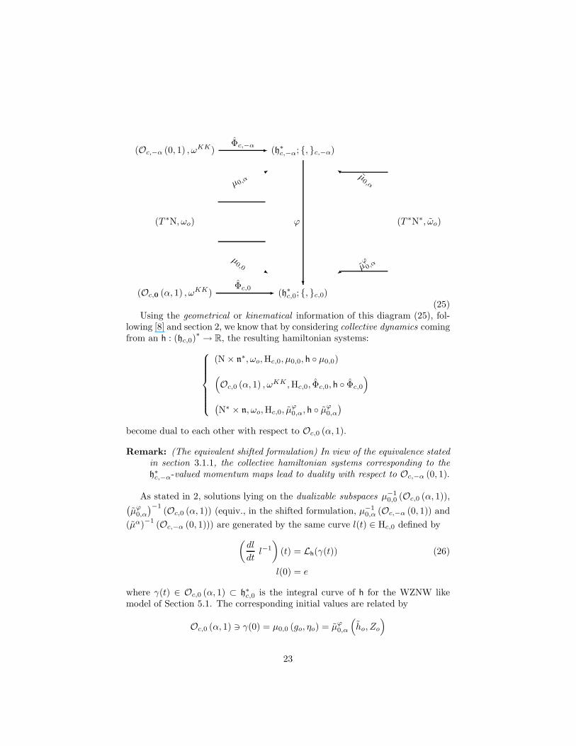
(25)Using the geometrical or kinematical information of this diagram (25), fol-

lowing [8] and section 2, we know that by considering collective dynamics comingfrom an h : (hc,0)

∗ → R, the resulting hamiltonian systems:

(N × n∗, ωo,Hc,0, µ0,0, h µ0,0)

(Oc,0 (α, 1) , ωKK ,Hc,0, Φc,0, h Φc,0

)

(N∗ × n, ωo,Hc,0, µ

ϕ0,α, h µϕ0,α

)

become dual to each other with respect to Oc,0 (α, 1).

Remark: (The equivalent shifted formulation) In view of the equivalence statedin section 3.1.1, the collective hamiltonian systems corresponding to theh∗c,−α-valued momentum maps lead to duality with respect to Oc,−α (0, 1).

As stated in 2, solutions lying on the dualizable subspaces µ−10,0 (Oc,0 (α, 1)),

(µϕ0,α

)−1(Oc,0 (α, 1)) (equiv., in the shifted formulation, µ−1

0,α (Oc,−α (0, 1)) and

(µα)−1

(Oc,−α (0, 1))) are generated by the same curve l(t) ∈ Hc,0 defined by

(dl

dtl−1

)(t) = Lh(γ(t)) (26)

l(0) = e

where γ(t) ∈ Oc,0 (α, 1) ⊂ h∗c,0 is the integral curve of h for the WZNW likemodel of Section 5.1. The corresponding initial values are related by

Oc,0 (α, 1) ∋ γ(0) = µ0,0 (go, ηo) = µϕ0,α

(ho, Zo

)

23

where (go, ηo) ∈ N × n∗ and(ho, Zo

)∈ N∗ × n stand for the initial conditions

for the N and N∗ sigma models of sects. 5.2 and 5.3, respectively. Thus, finally,the dual solutions can be written as:

d (l(t), (go, ηo)) ∈ N × n∗

[l(t)lo] ∈ Oc,0 (α, 1) ≃ H/Hα

b

(l(t),

(ho, Zo

))∈ N∗ × n

Notice that duality transformations between T ∗N and T ∗N∗ involve findingthe curve l(t) of (26) and applying the two factorizations H = N ⊲⊳ N∗ ∼ N∗ ⊲⊳N. As mentioned before, this duality transformations hold on the dualizablesubspaces described above.

Remark: (Plurality) In this context, it is clear that another decomposition[23] H = M ⊲⊳ M∗ of the same group shall yield plurality between thecorresponding collective models on M, M∗, N and N∗, as long as the mo-ment maps associated to the H-action intersect (recall sec. 2). Also noticethat, if P is another hamiltonian H-space whose moment map intersectsthe others, then a collective hamiltonian system on P will also be dualto the previous ones. In the first cases, being the phase spaces cotangentbundles T ∗N (T ∗N∗, etc.), it allows for a lagrangian description in termsof curves (or fields, see next sections) lying in N, (N∗, etc.).

5 Associated hamiltonian Systems

In the previous section, we have been concentrated on the kinematic-geometricaspects of Poisson Lie T -duality. In the current section, we describe the hamilto-nian systems’ equations associated to the dual phase spaces we have constructedendowed with the corresponding collective dynamics.

5.1 Master WZNW-type model on (T ∗H, ωc,θ)

The equation of motion on the phase space (T ∗H, ωc,θ) described in Section 3.1,for some H ∈ C∞ (H × h∗), are

l−1 l = δHη = ad∗δH

(η − Cθ

(l−1))

− cθ (δH) − ldH (27)

for (l, η) ∈ H × h∗, with dH|(l,η) = (dH, δH)(l,η) ∈ T ∗(l,η) (H × h∗). By setting

θ = 0 one gets the equation of motion for the system 1 (S1) and, for θ = −α,the equation of motion for the system 2 (S2), as described in that Section.

Collective dynamics warranties Lax type equations, so we consider someexamples with quadratic Hamilton functions including some arbitrary linear selfadjoint operators Li : h −→ h and L

∗i ≡ ψ Li ψ : h∗ −→ h∗, i = 1, 2, 3, where

24

ψ : h −→ h∗ denotes the identification induced by the symmetric Ad-invariantnon degenerate bilinear form (, )h, and ψ means the inverse map.

S1- For the symplectic manifold (H × h∗, ωc,0), and their reduced space M(α,1)c,0 ,

we consider

Hc,0 (l, η;α) =1

2(Ad∗l−1η,L∗

3Ad∗l−1η)h∗ + (Ad∗l−1η,L∗

2 (C−α (l) + α))h∗

(28)

− 1

2((C−α (l) + α) ,L∗

2 (C−α (l) + α))h∗

To realize the collective form of this hamiltonian function, we follow theresults of item S1 in Sec. 3.1 in order to restrict the system to the

Marsden-Weinstein reduced spaces M(α,1)c,0 . This means to make η =

Ad∗l C (l) + α and, because of the residual left action of H on H/Hα we

have the associated momentum map Φc,0 : H/Hα −→ h∗c,0, Φc,0 (l · Hα) =(C−α (l) + α, 1), which allow us retrieve the collective form

Hc,0 (l;α)|M

(α,1)c,0

=1

2

(Φc,0 (l · Hα) , (L∗

3 + L∗2) Φc,0 (l · Hα)

)

h∗

Hence, the Hamilton equations a restricted to

[JRc,0

]−1

(α, 1) =(l, AdH∗

l C (l) + α)/l ∈ H

arel−1 l = ψ

((Ll∗3 + L

l∗2

)η)

η = ad∗ψ((Ll∗

3 +Ll∗2 )η)

(η − α) − c(ψ((

Ll∗3 + L

l∗2

)η))

The Legendre transformation from the first equation leads to the la-grangian function Lc,0 =

⟨η, l−1g

⟩−Hc,0,

Lc,0 =1

2

⟨L∗3ψ(ll−1

), ll−1

⟩−⟨

L∗3L

∗2 (C−α (l) + α) , l−1 l

⟩

+1

2

((C−α (l) + α) ,

(L∗2 + L

∗2L

∗3L

∗2

)(C−α (l) + α)

)h∗

S2- For the symplectic manifold (H × h∗, ωc,−α) and their reduced spaceM(0,1)c,−α,

we consider the quadratic Hamilton functions

Hc,−α (l, η;−α) =1

2(Ad∗l−1η,L∗

3Ad∗l−1η)h∗ + (Ad∗l−1η,L∗

2C−α (l))h∗ (29)

− 1

2(C−α (l) ,L∗

2C−α (l))h∗

When restricted to M(0,1)c,−α, η = Ad∗lC−α (l), see item S2 in Sec. 3.1, it

takes the form

Hc,−α (l, η;−α)|M

(0,1)c,−α

=1

2(C−α (l) , (L∗

2 + L∗3)C−α (l))h∗

25

which is collective for the momentum map Φc,−α(l · Hc,−αˆ

α

)= (C−α (l) , 1).

The Hamilton equations of motion reduced to

[JRc,−α

]−1

(0, 1) =(l,−C−α

(l−1))/l ∈ H

arel−1 l = ψ

((Ll∗3 + L

l∗2

)η)

η = ad∗ψ(((Ll∗

3 +Ll∗2 )η))

η − c−α(ψ((

Ll∗3 + L

l∗2

)η))

We use the first equation of motion to invert the Legendre transformation

in order to obtain the lagrangian function Lc,−α =⟨η, l−1l

⟩− Hc,−α.

Thus, we get

Lc,−α(l, l)

=1

2

⟨L∗3ψ(ll−1

), ll−1

⟩−⟨

L∗3L

∗2C−α (l) , ll−1

⟩

+1

2

(C−α (l) ,

(L∗2 + L

∗2L

∗3L

∗2

)C−α (l)

)h∗

5.2 Collective hamiltonian on the factor (N × n∗, ωo)

5.2.1 Collective system for µ0,0 : N × n∗ −→ hc,0

Sigma models are now regarded as collective systems on N × n∗. T -dualityscheme can be applied to the hamiltonian space (N × n∗, ωo,Hc,0, µ0,0, h µ0,0), for an arbitrary function h : h∗c,0 −→ R.

For instance, a specific type of quadratic hamiltonian for µ0,0 : N × n∗ −→hc,0 was built up in [8] for N ≡ LG, so we refer to it and give here a brief recall.Using the invariant bilinear form (, )h we propose the collective hamiltonian

H0σ (g, η) =

1

2

(AdH

g η + C (g) , E(AdH

g η + C (g)))

h(30)

where E : h → h is a self adjoint linear operator. Motivated by standardPoisson-Lie T-duality [8], we further assume that E2 = Id. Now, followingAppendix 2, we call Eg = AdH

g−1EAdHg , Gg = (ΠnEgΠn∗)−1 : n −→ n∗ and

Bg = −Gg ΠnEgΠn : n −→ n∗. Then, Hamilton equation for g ∈ N is

g−1g = (Gg)−1 BgC(g−1

)+ (Gg)−1 η

The lagrangian coming from the collective hamiltonian given by such symmetricoperator E defines a sigma model since, as a block matrix in g ⊕ g∗, we have

Eg =

(−G−1

g Bg G−1g

Gg − BgG−1g Bg BgG−1

g

)(31)

Following ref. [8] we arrive to the sigma model lagrangian (see also Appendix2),

L0σ =

1

2

⟨(Gg + Bg)

(g−1g − C

(g−1

)), g−1g + C

(g−1

)⟩. (32)

26

5.2.2 Collective system for µ0,α : N × n∗ −→ h∗c,−α

Let us now consider the hamiltonian space (N× n∗, ωo,,Hc,−α, µ0,α, h ϕµ0,α)where µ0,α : N × n∗ −→ h∗c,−α was defined in (18) for α satisfying condition(17), ϕ : h∗c,−α −→ h∗c,0 is the Poisson diffeomorphism introduced in 3.1.1. Forh being the quadratic function as in (30), we have

Hασ = h ϕ µ0,α =

1

2(ϕ µ0,α, Eϕ µ0,α)

h

The non degenerate symmetric bilinear form (, )h induces the identification ψbetween h and h∗, so that the hamiltonian turns out to be

Hασ =

1

2

(ϕ AdH∗

−α;g−1 (ψ (λ) , 1) , Eψ(ϕ AdH∗

−α;g−1 (ψ (λ) , 1)))

h

Hamilton equations of motion yield

g−1g = Πnψ(Eg(λ+AdH

g−1 ψ (C (g)) + α))

Taking into account the form of the operator Eg of eq. (31),

g−1g = G−1g BgC

(g−1

)+ G−1

g (λ+ α)

Once again, to retrieve the lagrangian function, we use the first Hamilton equa-tion to invert the Legendre transformation

λ = Ggg−1g − BgC(g−1

)− α

Thus, by Appendix 2,

Lασ =1

2

((Gg + Bg)

(g−1g − C

(g−1

)), g−1g + C

(g−1

))h−⟨g−1g, α

⟩.

5.3 Collective hamiltonian on the factor (N∗ × n, ωo)

Let us now consider the collective dynamic system on T ∗N∗ ∼= N∗ × n definedby,

Hα = h µϕ0,αfor the momentum map µϕ0,α : N∗ × n −→ h∗c,0, defined in (21), and h being thequadratic function as above. This yields

Hα =1

2

(AdD

h(X + α) + C

(h), E(AdD

h(X + α) + C

(h)))

h

so that the Hamilton equation of motion for h is

h−1

h = Eh(X + α− C

(h−1

))

27

where Eh = AdHh−1

EAdHh. Using the dual decomposition h⊤ = n∗ ⊕ n, we can

write

Eh =

(−G−1

hBh G−1

h

Gh − BhG−1

hBh BhG−1

h

)

with the operators Gh = (Πn∗EhΠn)−1 : n∗ −→ n and Bh = −Gh Πn∗EhΠn∗ :

n∗ −→ n. The equation for h yields

X = Gh

(h−1

h

)+ Bh

(α− C

(h−1

))

We thus obtain, following Appendix 2, the following lagrangian function

Lα(h,

h

)=

1

2

(h−1

h+ C(h−1

)− α,

(Gh + Bh

)(h−1

h− C(h−1

)+ α

))

Remark: (The equivalent shifted formulation) Analogously, a model on T ∗N∗ ∼=N∗ × n in corresponding shifted version can be obtained by proposing ahamiltonian function

Hα = h ϕ µα

for µα : (N∗ × n, ωo) −→ (h, , Affc,−α) defined in eq. (24), leading to thesame Hamilton equations and lagrangian since ϕ µα = µϕ0,α.

6 Loop groups and Poisson Lie T-duality for

trivial monodromies

In the classical field theory context, Sigma and WZNW models can be builtup on the cotangent bundle of loop groups. In particular, for the WZNWmodel, a pure cocycle is added to the canonical symplectic form in order toproduce the decoupling of the chiral modes [12], leading to the fact that a generalsolution for the equation of motion can be written as a non linear combination ofboth modes. Finally, on the chiral phase space, solutions related to non-trivialextended coadjoint orbits are the ones associated to non trivial monodromies.

In this Section, we apply the results obtained in the previous sections to thecase of underlying loop groups, thus addressing the case in which non trivialmonodromies appear. More precisely, we consider H = LD, for some Lie groupD with Lie algebra d such that h = Ld. Moreover, d will be regarded also as adouble Lie group D = G ⋊⋉ G∗ with Lie bialgebra d = g ⊕ g, so that N = LG,n = Lg, and the same for the corresponding duals.

For l ∈ LD, l′ denotes the derivative in the loop parameter s ∈ S1, and wewrite vl−1 and l−1v for the right and left translation of any vector field v ∈ TD.Let d be the Lie algebra of D equipped with a non degenerate symmetric Ad-invariant bilinear form (, )d. Frequently we will work with the subset Ld∗ ⊂

28

(Ld)∗ instead of (Ld)∗ itself, and we identify it with Ld through the map ψ :Ld → Ld∗ provided by the bilinear form

(, )Ld ≡ 1

2π

∫

S1

(, )d

on Ld. In this framework, the two cocycle c : h× h −→ R of Section 3.1 is givenby the bilinear form Γk : Ld × Ld → R [11],

c(X,Y) ≡ Γk(X,Y) =k

2π

∫

S1

(X (s) ,Y′ (s))d ds

with X,Y ∈ Ld. It is derived from the one cocycle Ck : LD → Ld∗,

Ck (l) = kψ(l′l−1

).

As in section 3, when the corresponding central extension LDΓkof LD does

exist, the centrally extended affine adjoint and coadjoint actions of LDΓkon

LdΓkand Ld∗Γk

are defined as

Ad∗

l−1 (ξ, b) =(Ad∗l−1ξ + bkψ

(l′l−1

), b)

Note that the S1 ⊂ LDΓkaction is trivial and the embedding ξ → (ξ, 1) is a

Poisson map from Ld∗Aff to LdΓk∼ Ld × R which maps the affine coadjoint

action of LD to the centrally extended one of LD → LDΓk.

We now recall some facts about the stabilizer subgroup of a point (η, 1) ∈Ld∗Γk

. If [LD](η,1) denotes the stabilizer, with η ∈ Lg∗, consider hη (s) ∈C∞ (R, G∗), hα (0) = e, and Mη ∈ G∗ such that

η (s) = h′η (s) h−1η (s)

hη (s+ 2π) = hη (s) Mη

where Mη ∈ G∗ is the monodromy of the g∗-valued map η (s). Then [LD](η,1)consists of loops of the form

l (s) = hη (s) l (0) h−1η (s)

based at some point l (0) within the stabilizer DMηof Mη in D

Mη = l−1 (0) Mηl (0)

For any other point (β, 1) = AdLD∗

m (η, 1) ∈ O (η, 1), m ∈ LD, the isotropygroup is m−1

(LD(η,1)

)m. Writing β (s) = −l′β (s) l−1

β (s) with monodromy

Mβ = l−1β (s) lβ (s+ 2π), it is related with Mη as

Mβ = m−1 (s) Mηm (s)

29

As a symplectic manifold, the coadjoint orbit OΓk,0(α, 1) ⊂ Ld∗Γk,0passing

through (α, 1) ∈ Ld∗Γk,0, for α ∈ Lg∗, is endowed with the Kirillov-Kostant

symplectic form⟨ωαKK , ad

∗

(X,a)(β, 1) ⊗ ad∗

(Y,b)(β, 1)⟩

(β,1)= 〈[X,Y], β〉 + Γk(X,Y)

with (β, 1) = AdLD∗

l (α, 1) ∈ OΓk,0(α, 1), for some l ∈ LD.Let us define

φ : LD −→ OΓk,0(α, 1) ⊂ Ld∗Γk

φ(l) = AdLD∗

l (α, 1)

(33)

and consider the pull back of ωαKK through φ

φ∗ωαKK |l = Γk(l−1dl⊗, l−1dl) +

⟨α, [l−1dl⊗, l−1dl]

⟩

The null distribution of this form is spanned by the Lie algebra of the stabilizersubgroup LD(α,1) of (α, 1). Thus, if LD/LD(α,1) is a smooth manifold, there is

a symplectic diffeomorphism (LD/LD(α,1), φ∗ωαKK)

φ−→ (OΓk,0(α, 1), ωαKK).As a consequence we have,

Remark: The momentum map associated to the residual symmetry of LD onLD/ [LD](α,1) is φ.

By also recalling the map µ0,0 from [8] (called just µ there), so far we have

T ∗LG

LD/LDα(x)∼= OΓk,0(α, 1)

φ- Ld∗Γk,0

µ0,0

-(34)

We are going now to describe the other phase spaces presented in section 3which are also related to the orbit OΓk,0(α, 1).

6.1 The chiral WZNW phase space

The phase spaces described in section 5.1, for H = LD, correspond to a chiralsector of the WZNW model [21]. Consider the unique curve hα ∈ C∞ (R, G∗)such that

α (s) = h′α (s) h−1α (s)

with hα (0) = e so that hα (2π) = Mα = Hol(α(s)) is the holonomy of α(s) ⊂ g∗.The solutions in LD to the classical equation of motion of the WZNW model

∂−(∂+l l−1) = 0

are l(s, t) = lL(x+)l−1R (x−), which combines the chiral solutions lL(x−) and

lR(x+), with x± = s ± t. In spite of the fact that l(s, t) is periodic in s, the

30

chiral modes are not restricted to be closed loops. In fact, for chiral modessatisfying

l LR

(x± + 2π) = l LR

(x±) M

the solutions l(s, t) remains periodic. Let PD be the extended chiral phase spaceof the WZNW model (see [21])

PD = l : R −→ D / l(x+ 2π) = l(x)M, for some M ∈ D.

Here, each M ∈ D is the monodromy of path l(x) satisfying

l(0)Ml−1(0) = Hol(l′l−1) = l(2π)l−1(0)

since l(0)−1l(2π) = M .In order to study separately the chiral degree of freedom, the following sym-

plectic form on PD must be considered

ωPD(l) = −Γk(l−1dl⊗, l−1dl) − 1

2

⟨(l−1dl)(0)∧, dMM−1

⟩+ ρ(M)

with ρ being a 2-form just depending on the holonomy M so that

dρ(M) =1

6

⟨dMM−1∧, [dMM−1∧, dMM−1]

⟩

It is worth to remark that ρ is defined just locally in some neighborhood ofthe identity. In ref. [21], it is shown that such ρ is given by generalized rmatrices solutions of the Generalized Dynamically Modified Classical Yang-Baxter equation, defining Poisson structure chiral space PD.

Let us define the map

J : PD −→ Ld∗Γk

J(l) = (l′l−1, 1)(35)

The loop group LD acts on PD by left multiplication with associated momen-tum map J . On the other side, the group D acts on PD by right multiplication

l(x)d−→ l(x).d, which is a Poisson-Lie symmetry in relation to the Poisson-

Lie structure on D given by the canonical r-matrix in the double Lie algebrad and a particular election of ρ(M), as it is shown in [21]. In that case, themap σ : LD −→ D∗ defined as σ(l(x)) = l−1(x)l(x + 2π) = M defines thecorresponding D∗-valued momentum map.

Then, we have the following diagram

PD

Ld∗Γk

J

D∗

σ

-

31

For each value M , we consider the pre image σ−1(M) ⊂ PD and define thesubspace

Eα(D) = LD · hα = l · hα / l ∈ LDwhich is injected into σ−1(M) ⊂ PD as follows

Eα(D)i→ σ−1(M = Hol(α)) ⊂ PD.

Because it can be identified with LD, the restriction of the symplectic form onPD to Eα(D) coincides with µα∗ωαKK |l, and

µα := J i

is a presymplectic map. Hence, we have following phase spaces related by sym-plectic morphisms with the orbit OΓk,0(α, 1),

T ∗LG Eα(D)

µ0,0 -

OΓk,0(α, 1) →(Ld∗Γk,0, KK)

µα

?

6.2 A symplectic LD action on LG∗ × Lg

From Section 3.2.2, it follows that µϕ0,α : (LG∗ × Lg, ωo) −→ (Ld, , Aff) ⊂(Ld∗Γk,0

, , KKΓk,0

), given by

µϕ0,α(g, Z) = (g′g−1 +AdLDg (Z + α)) , (36)

is a Poisson map provided that condition (17) is satisfied. In the current loopgroup case, this means that

addα(s)X ∈ g ⊂ d (37)

for all X ∈ g and all s ∈ S1.

Remark: When G∗ = K is a compact simple real Lie group, e.g. SU(N), anyconstant element α ∈ t, where t is the Cartan subalgebra of k = Lie(K),condition (37) is satisfied (see Appendix 1).

Under this condition, the loop group LD acts on LG∗ × Lg via

(g, Z)l=ba7−→ (bga, AdLDag (Z + α) + (ag)′(ag)−1 − α)

32

where gaag = ag. The corresponding infinitesimal generator XLG∗×Lg|(g,Z) ∈T(g,Z)(LG

∗ × Lg) associated to an X = (ξ,X) ∈ Ld at the point (g, Z) ∈LG∗ × Lg is

XLG∗×Lg|(g,Z)

=(gΠg∗(AdLDg−1X),Πg

(AdLDg−1X′ −

[g−1g′ + Z + α,Πg(AdLDg−1X)

]))

where Πg∗ ,Πg are the projectors on the Lie subalgebras g∗, g, respectively.Moreover, this action is hamiltonian and the corresponding moment map isprecisely µϕ0,α.

6.3 T-duality diagram for non trivial monodromies

Thus, considering the results of this section, we may assemble a PL T -dualitydiagram based on the coadjoint orbit OΓk,0(α, 1) ⊂ Ld∗Γk,0

.This fact doesn’t affect the side corresponding to the phase space T ∗LG:

there we have a σ-model describing the dynamics of a closed string valued onthe target G, symmetric under the hamiltonian action of the group LDΓk,0 givenin eq. (13)and with associated momentum map µ0,0 of Proposition (3.2.1), asdepicted in diagram (34).

The double Lie group LD appears in T -duality diagrams through the sub-space Eα(D) bringing the open string models into the scheme. It is injected inthe extended chiral phase space of the WZNW model, PD, and relates to theorbit

(Ld∗Γk,0

, , KKΓk,0

)by the map µα := J i.

Finally, on the dual side things become subtler: as explained just above, andin section 3.2.2, the connection of the cotangent bundle T ∗LG∗ ∼= LG∗ × Lg tothe coadjoint orbit

(Ld∗Γk,0

, , KKΓk,0

)does exist provided α be such that (37) is

fulfilled. Under this condition, the map µϕ0,α : (LG∗×Lg, ωo) −→ (Ld, , Aff) ⊂(Ld∗Γk,0

, , KKΓk,0

)turns in a Poisson one, enabling to assemble the complete T -

duality diagram

T ∗LG Eα(D) T ∗LG∗

µ0,0 - µ

ϕ0,α

OΓk,0(α, 1) →(Ld∗Γk,0; , KKΓk,0)

µα

?

6.4 Induced hamiltonian systems on loops groups

Following section 5, we now choose a quadratic hamiltonian functionH : Ld∗c,0 ∼Ldc,0 −→ R given by

H(X, 1) =1

2〈X, E(X)〉

33

with E : d −→ d a linear operator. The lifts to LD/Dα(x) and PD are, respec-tively,

H φ(l) = 12

⟨Ad

∗

l (α, 1), E(Ad∗

l (α, 1))⟩

H J(l) = 12

⟨l′l−1, E(l′l−1)

⟩

We notice that H J in PD is invariant under the right (PL) action of Dand then, the corresponding momentum map shall give conserved quantities.This implies that the monodromy M is constant and that we can restrict to thesubspace within m−1(M) ⊂ PD consisting of paths with the same monodromy,for example Eα(D) defined above. The resulting dynamics is the chiral WZNW-type one corresponding to section 5.1.

In Ld∗c ∼ Ldc, writing the corresponding integral curve as γ(t) = Ad∗

l(t)(α, 1)for the initial value γ(0) = (α, 1), we have that the corresponding equation forl(t) ∈ LD is

d

dtll−1 = E(l ′l−1 +Adlα) = E((lb)′(lb)−1) (38)

l(t = 0) = e

with α = b′b−1, b(0) = e, b ∈ PG∗ ⊂ PD. Since the hamiltonian functions arein collective form (recall sec. 4.2), the integral curves in LD/Dα(x) and PD willbe determined by l(t).

Remark: (dual factorizations) Writing l = gh or l = gh, we alternativelyobtain

d

dtgg−1 +Adg

d

dthh−1 = E(g′g−1 + Adg(Adehα+ h′h−1))

= E( (ghb)′(ghb)−1)

d

dtgg−1 +Adg

d

dthh−1 = E(g′g−1 + Adg(Adhα+ h′h−1))

= E((ghb)′(ghb)−1).

In the first case, since α ∈ g∗ and, thus, b ∈ G∗, the terms correspondingto fields in G and G∗ split, allowing to lift the dynamics from OΓk,0(α, 1)to LT ∗G via µ, as we already knew [8]. In turn, in the second case above,this cannot be done generally because the G and G∗ variables are mixedup.

Now, if (37) is satisfied for a constant α ∈ g∗, following Sections 5.3 and 4.2,we find that the resulting model pulls back to (LG∗ ×Lg, ωo, h µϕ0,α) and that

34

it becomes dual to that on LT ∗G. The equations of motion on LG∗ × Lg are

g−1 d

dtg = ΠG∗(Eg(g−1g′ + Z + α))

d

dtZ = ΠG[Z, g−1 d

dtg] + EgadDg−1g′(Z + α) + Eg(g−1g′ + Z + α)′

− adDg−1g′Eg(g−1g′ + Z + α) − adD(Z+α)Eg(g−1g′ + Z + α)

whose solutions are given by

(g, Z)(t) = lt · (g0, Z0)

when lt ∈ LD is a solution of equation (38) and (g0, Z0) ∈ (µϕ0,α)−1(α, 1).

6.4.1 The induced lagrangians

The action functional corresponding to the above dynamics in LD/Dα(x), ex-pressed in terms of D-valued field l, is

S =

∫θα(l) −H φ(l)

where H is the hamiltonian given in the previous section and θα is a potentialfor the 2-form ωαKK , which can be written as

θα(l) =⟨l′l−1, dll−1

⟩+

1

6d−1

⟨dll−1, [dll−1, dll−1]

⟩+ 2

⟨l−1dl, α

⟩.

This agrees with the action proposed in ref. [22] for a particular choice of H .By construction, this WZW-like model on D is dual to the corresponding sigmamodels with targets G and G∗, as described in the previous sections.

The sigma model on G, for a particular choice of E , can be found in ref. [8].The same operator E , following section 5.3 and assuming (37) is satisfied for aconstant α ∈ g∗, induces a lifted hamiltonian on (LG∗ ×Lg, ωo). The Legendretransformation turns out to be non singular and the resulting model is given bythe lagrangian (see Appendix 2)

Lα(g,dg

dt) =

⟨∂−gg

−1 −AdDg α, ((Be + Ge) + π(g))−1

(∂+gg−1 +AdDg α)

⟩(39)

where π(g) is the Poisson bivector of G∗. Using the fact that π(g) = π(gexα)since (37) is satisfied, then this lagrangian can be expressed in terms of the openmonondromic string variable m = gexα, x ∈ [0, 2π],

Lα(m,dm

dt) =

⟨∂−mm

−1, ((Be + Ge) + π(m))−1∂+mm

−1⟩

35

Remark: This lagrangian corresponds to the one given in [22], but in our casewe know by construction that the dynamics preserves the monodromy (it

restricts to(µϕ0,α

)−1(OΓk,0(α, 1)) ⊂ LG∗ × Lg when the initial value lies

there) and no further constraints are needed.

In the above case, for each α we have a dual model Lα. One may ask if wecan glue all this models together making a unique L which is dual to the one inG for any α. Note that to that end, we should consider α as varying in a spaceof all possible (log of) monodromies t (e.g.: in a torus t inside a compact groupK [22]) and then consider a structure on LG∗ × Lg × α giving the correctdynamics.

If α ∈ t is considered as a variable, the correct dynamics is given by one whichsets α = const. To that end, we enlarge the phase space from LG∗ × Lg to the(also symplectic) (LG∗ × Lg × T ∗t, ωo(g, Z) ⊕ ωo(α, λ)). There, we define

µ : LG∗ × Lg × T ∗t −→ Ld

: (g, Z, α, λ) 7→ g′g−1 +AdDg (Z + α)

which is still a Poisson map. The action it generates is the same on LG∗ × Lg,it is trivial on t and is non trivial on t∗. Now, the image of µ covers all the orbitsOΓk,0(α, 1) for α ∈ t.The lagrangian associated to the (now singular since h µdoes not depend on λ) hamiltonian system (LG∗ × Lg × T ∗t, ωo ⊕ ωo, h µ) is

L(g, ∂g∂t , α,∂α∂t , λ)

=⟨(∂−g) g

−1 −AdDg α, ((Be + Ge) + π(g))−1

((∂+g) g−1 +AdDg α)

⟩+

⟨λ,∂α

∂t

⟩

where in the last added term λ plays the role of a Lagrange multiplier, and sothe dynamics for the new variables is

∂α

∂t= 0

∂λ

∂t= ∇αLα.

Example: (Lu-Weinstein doubles) Let K be a real simple and compact Liegroup. Then D = AN×K where G = AN and G∗ = K are the subgroupsgiven by the Iwasawa decomposition of KC. Now, let T ⊂ K be a maximaltorus and t its Lie algebra. By choosing a constant α ∈ t and a particularhamiltonian on Ld∗c , we obtain a resulting model in phase space (LG∗ ×Lg, ωo). This model can be expressed in terms of g(x).exα exclusively,yielding a monodromic strings model similar to that of [22]. This followsfrom the above considerations because, in this case, b = exα and ghb =

(gb)(hb) (see Appendix 1). The resulting lagrangian is (39) (compare tothe ad hoc constrained one of [22]).

36

7 Conclusions

We carried out an enlargement of the T -duality scheme developed in [8] in orderto include coadjoint orbits with non trivial monodromy as pivotal phase space.To that end, we considered a general framework for studying duality betweendifferent phase spaces which share the same symmetry group H. Solutionscorresponding to collective dynamics become dual in the sense that they aregenerated by the same curve in H. Explicit examples of dual phase spaces inthe above sense were constructed on the cotangent bundles of the factors of adouble Lie group H = N ⋊⋉ N∗.

When considering duality over non trivial extended orbits Oc,0 (α, 1) withα ∈ n∗, some important new facts appeared, being the most significative theloss of the symmetry between the role played by the factors of the double Liegroup. Also, a condition on α, eq. (17), has to be imposed in order for themomentum maps intersecting in Oc,0 (α, 1) to be compatible with the underly-ing hamiltonian structure (i.e. to be Poisson maps). In the loop group case,standard sigma models are now T-dually related to models with non trivial α-monodromies, namely open string models [22], as showed in subsection 6.4.1. Itis worth to remark that, in the present framework, the dynamics of open stringmodels are monodromy preserving by construction, no further constraints needto be added.

On the other hand, since a non trivial orbit becomes related to a trivialone by changing the cocycle extension by coboundary, we introduced a secondpivotal vertex in the T-duality scheme. This trivial orbit can be regarded asthe phase space chiral modes of a WZNW type model, with shifted collectivelagrangian, and allows for additional collective models on the cotangent bundlesof the factors N and N∗ in the T-duality class of those hanged from the nontrivial monodromy orbit.

Thus, we succeeded in to generalize the symplectic geometry approach toPoisson Lie T-duality of ref. [8], stressing the fundamental role played by coad-joint orbits of double Lie groups, central extensions and collective dynamics,also analyzing some hamiltonian an lagrangian models on the involved phasespaces.

8 Appendix 1

We are going to study the structure of the brackets in the double Lie algebrafor g being a simple compact real Lie algebra (e.g. su(n)). Recall from [24],that if (Hi, ei, fi) with i = 1, ..., rank(g) denotes the elements of the Chevalleybasis of g for a fixed Borel subalgebra b, then

[Hi, Hj ] = 0 (40)

[Hi, ej ] = aijej

[Hi, fj ] = −aijfj

37

where (aij) denotes the Cartan matrix of g. Note that spanHi is the abelian

Lie algebra of a maximal torus T ⊂ G. The standard bialgebra structure δ :g −→ g ∧ g on g is defined by

δ(Hi) = 0 (41)

δ(ei) = diHi ∧ eiδ(fi) = diHi ∧ fi

with di being the length of the i-th. root.Now, let (Hi, ei, f i) denote the basis of g = g∗ dual to (Hi, ei, fi). We want

to express the commutation relations in terms of this dual basis of the bracketon g induced by δ. Using (40), (41) and the definition

〈[X,Y ], α〉 = 〈X ⊗ Y, δ(α)〉

for all X,Y ∈ g, α ∈ g, it is easy to see that in g

〈[X,Y ], Hi〉 = 0.

Thus, in the double d = g ⊕ g, we have that

[(Hi, 0), (0, X)]d = (0, ad∗HiX)

hence, if b = exp(ΣiciHi) ∈ T ⊂ G, h ∈ G,

b · h = hb · b

so the dressing action of h on b is trivial, i. e. bh = b.

9 Appendix 2

Here we give some details on the algebra involved in passing from a 1st. orderlagrangian to a 2nd. order sigma model lagrangian.

Let us start with a 1st. order lagrangian, q, q ∈ V , p ∈ V,

L(q, p) = 〈p, q〉 − 1

2〈p+ q, E(p+ q)〉

for E linear operator on V⊕ V satisfying E2 = Id and being self adjoint withrespect to the pairing 〈, 〉. From these conditions, it is easy to see that theoperator G−1 := ρV EρV : V −→ V is invertible and that

〈Gv, w〉 = 〈v,Gw〉

v, w ∈ V . Also, B := (ρV EρV ) (ρV ∗EρV )−1 : V −→ V satisfies

〈Bv, w〉 = −〈v,Bw〉

38

with ρV , ρV denoting the projections on V and V , respectively. We also havethe relations

ρV EρV = −G−1BρV EρV = G − BG−1B.

Euler-Lagrange equations for the variable p imply

∂L

∂p= 0

q = E(p+ q)

thus,p = Gq + Bq.

Hence, using the above equations to rewrite the lagrangian in terms of q, q weobtain

L(q, q) =1

2〈q,Gq〉 − 1

2〈q,Gq〉 − 〈q,Bq〉

=1

2〈q − q, (G + B)(q + q)〉

the sigma model like 2nd. order lagrangian.

Acknowledgments

H.M. and A.C. thanks to CONICET for financial support.

References

[1] C. Klimcik, P. Severa, Poisson-Lie T-duality and loop groups of Drinfelddoubles, Phys. Lett. B 351, 455-462 (1995), hep-th/9512040; Dual non-Abelian duality and the Drinfeld double, Phys. Lett. B 372, 65-71 (1996),hep-th/9502122; Poisson-Lie T-duality; C. Klimcik, Nucl. Phys. Proc.Suppl. 46, 116-121 (1996), hep-th/9509095.

[2] Y. Lozano, Non Abelian duality and canonical transformations, Y. Lozano,Phys. Lett. B 355, 165-170 (1995), hep-th/9503045.

[3] A. Yu. Alekseev, A. Z. Malkin, Symplectic structures associated to Lie-Poisson groups, Comm. Math. Phys. 162, 147-74 (1994), hep-th/9303038.

[4] O. Alvarez, Target space duality I: general theory, Nucl. Phys. B 584 (2003)659-681, hep-th/0003177; Target space duality II: applications, Nucl. Phys.B 584, 682-704 (2003), hep-th/0003178.

39

[5] K. Sfetsos, Canonical equivalence of non-isometric sigma-models andPoisson-Lie T-duality, Nucl. Phys. B 517, 549-566 (1998), hep-th/9710163;Poisson Lie T-duality beyond the classical level and the renormalizationgroup Phys. Lett. B 434, 365-375 (1998), hep-th/9803019.

[6] A. Stern, Hamiltonian approach to Poisson Lie T-duality, Phys. Lett. B450, 141-148 (1999), hep-th/9811256.

[7] A. Yu. Alekseev, C. Klimcik, A.A. Tseytlin, Quantum Poisson-LieT-duality and WZNW model, Nucl. Phys. B 458, 430-444 (1996),hep-th/9509123.

[8] A. Cabrera, H. Montani, Hamiltonian loop group actions and T -Dualityfor group manifolds, J. Geom. Phys. 56, 1116-1143 (2006).

[9] Coste, A., Dazord, P. and Weinstein, A., Groupoıdes symplectiques, Pub-lications du Departement de Mathematiques de l’Universite de Lyon, I,2/A, 1-65 (1987); Mikami, K., and Weinstein, A., Moments and reduc-tion for symplectic groupoid actions, Publ. RIMS Kyoto Univ. 24, 121-140(1988).

[10] J. E. Marsden, A. Weinstein, Reduction of symplectic manifolds with sym-metry, Rep. Math. Phys. 5, 121-131 (1974).

[11] A. Pressley, G. Segal, Loop groups, Oxford: Clarendon Press, 1986.

[12] J. Harnad, Constrained hamiltonian systems on Lie groups, moment mapreductions and central extensions, Can. J. Phys. 72, 375-388 (1994) ; John

Harnad, B. A. Kupershmidt, Symplectic Geometries on T ∗G, hamiltonianGroup Actions and Integrable Systems, J. Geom. Phys. 16, 168-206 (1995).

[13] V. G. Drinfeld, Hamiltonian Lie groups, Lie bialgebras and the geometricmeaning of the classical Yang Baxter equation, Soviet Math. Dokl. 27, 68(1983).

[14] J.-H. Lu, A. Weinstein, Poisson Lie groups, dressing transformations andBruhat decomposition, J. Diff. Geom. 31, 501-526 (1990).

[15] M.A. Semenov-Tian-Shansky, Dressing transformations and Poisson groupactions, Publ. RIMS, Kyoto Univ. 21 (1985), 1237-1260.

[16] V. Guillemin, S. Sternberg, Symplectic technics in physics, Cambridge,Cambridge Univ. Press, 1984.

[17] D. Kazhdan, B. Kostant , S. Sternberg, Hamiltonian group actions anddynamical system of Calogero type, Commun. Pure Appl. Math. 31, 481-508 (1978).

[18] J. Marsden, T. Ratiu, Introduction to Mechanics and Symmetry, SpringerVerlag 1994.

40

[19] C. Klimcik, Quasitriangular WZW model, Rev. Math. Phys.16, 679-808,(2004), hep-th/0103118.

[20] C. Klimcik, S. Parkhomenko, Supersymmetric gauged WZNW modelsas dressing cosets, Phys.Lett. B 463, 195-200 (1999), hep-th/9906163;S.E.Parkhomenko, Poisson-Lie T-duality and Complex Geometry in N=2superconformal WZNW models, Nucl.Phys. B 510, 623-639 (1998),hep-th/9706199; C. Klimcik, Poisson-Lie T-duality and (1,1) supersym-metry, Phys.Lett. B 414, 85-91 (1997), hep-th/9707194.

[21] J. Balog, L. Feher, L. Palla, Chiral Extensions of the WZNW PhaseSpace, Poisson-Lie Symmetries and Groupoids, Nucl.Phys. B568 (2000)503-542, e-Print Archive: hep-th/9910046; L. Feher, I. Marshall, Thenon-Abelian momentum map for Poisson-Lie symmetries on the chiralWZNW phase space, math.QA/0401226; J. Balog, L. Feher, L. Palla,On the Chiral WZNW Phase Space, Exchange r-Matrices and Poisson-LieGroupoids, Talk given at the Superior Mathematics Seminar, Montreal,Quebec, Canada, 26 Jul - 6 Aug 1999, e-Print Archive: hep-th/9912173.

[22] C. Klimcik, S. Parkhomenko, Monodromic strings, hep-th/0010084 ; C.Klimcik, S.E. Parkhomenko, The Poisson-Lie T-duality and zero modes,Theor. Math. Phys.139:834-845, (2004).

[23] L. Hlavaty, L. Snobl, Poisson-Lie T-plurality of three-dimensional confor-mally invariant sigma models, JHEP 0410:045, (2004), hep-th/0403164.

[24] V. Chari, A. Pressley, A Guide to Quantum Groups, Cambridge UniversityPress 1994.

41