Sequences and Difference Equations
238
Sequences and Difference Equations A From mathematics you probably know the concept of a sequence , which is nothing but a collection of numbers with a specific order. A general sequence is written as x 0 ,x 1 ,x 2 , ..., x n , .... One example is the sequence of all odd numbers: 1, 3, 5, 7,..., 2n +1, .... For this sequence we have an explicit formula for the n-th term: 2n +1, and n takes on the values 0, 1, 2,... . We can write this sequence more compactly as (x n ) ∞ n=0 with x n =2n + 1. Other examples of infinite sequences from mathematics are 1, 4, 9, 16, 25, ... (x n ) ∞ n=0 ,x n =(n + 1) 2 , (A.1) 1, 1 2 , 1 3 , 1 4 , ... (x n ) ∞ n=0 ,x n = 1 n +1 . (A.2) The former sequences are infinite, because they are generated from all integers ≥ 0 and there are infinitely many such integers. Neverthe- less, most sequences from real life applications are finite. If you put an amount x 0 of money in a bank, you will get an interest rate and therefore have an amount x 1 after one year, x 2 after two years, and x N after N years. This process results in a finite sequence of amounts x 0 ,x 1 ,x 2 ,...,x N , (x n ) N n=0 . Usually we are interested in quite small N values (typically N ≤ 20 − 30). Anyway, the life of the bank is finite, so the sequence def- initely has an end. H.P. Langtangen, A Primer on Scientific Programming with Python, Texts in Computational Science and Engineering 6, DOI 10.1007/978-3-642-30293-0, c Springer-Verlag Berlin Heidelberg 2012 557
-
Upload
khangminh22 -
Category
Documents
-
view
2 -
download
0
Transcript of Sequences and Difference Equations

Sequences and Difference Equations A
From mathematics you probably know the concept of a sequence, whichis nothing but a collection of numbers with a specific order. A generalsequence is written as
x0, x1, x2, . . . , xn, . . . .
One example is the sequence of all odd numbers:
1, 3, 5, 7, . . . , 2n+ 1, . . . .
For this sequence we have an explicit formula for the n-th term: 2n+1,and n takes on the values 0, 1, 2, . . . . We can write this sequence morecompactly as (xn)
∞n=0 with xn = 2n + 1. Other examples of infinite
sequences from mathematics are
1, 4, 9, 16, 25, . . . (xn)∞n=0, xn = (n+ 1)2, (A.1)
1,1
2,1
3,1
4, . . . (xn)
∞n=0, xn =
1
n+ 1. (A.2)
The former sequences are infinite, because they are generated fromall integers ≥ 0 and there are infinitely many such integers. Neverthe-less, most sequences from real life applications are finite. If you putan amount x0 of money in a bank, you will get an interest rate andtherefore have an amount x1 after one year, x2 after two years, and xNafter N years. This process results in a finite sequence of amounts
x0, x1, x2, . . . , xN , (xn)Nn=0.
Usually we are interested in quite small N values (typically N ≤20− 30). Anyway, the life of the bank is finite, so the sequence def-initely has an end.
H.P. Langtangen, A Primer on Scientific Programming with Python,Texts in Computational Science and Engineering 6,
DOI 10.1007/978-3-642-30293-0, c© Springer-Verlag Berlin Heidelberg 2012
557

558 A Sequences and Difference Equations
For some sequences it is not so easy to set up a general formula forthe n-th term. Instead, it is easier to express a relation between two ormore consecutive elements. One example where we can do both thingsis the sequence of odd numbers. This sequence can alternatively begenerated by the formula
xn+1 = xn + 2. (A.3)
To start the sequence, we need an initial condition where the value ofthe first element is specified:
x0 = 1.
Relations like (A.3) between consecutive elements in a sequence is calledrecurrence relations or difference equations . Solving a difference equa-tion can be quite challenging in mathematics, but it is almost trivialto solve it on a computer. That is why difference equations are so wellsuited for computer programming, and the present appendix is devotedto this topic. Only programming concepts from Chapters 1–5 are usedin the material herein.
The program examples regarding difference equations are found inthe folder src/diffeq.
A.1 Mathematical Models Based on Difference Equations
The objective of science is to understand complex phenomena. Thephenomenon under consideration may be a part of nature, a group ofsocial individuals, the traffic situation in Los Angeles, and so forth. Thereason for addressing something in a scientific manner is that it appearsto be complex and hard to comprehend. A common scientific approachto gain understanding is to create a model of the phenomenon, anddiscuss the properties of the model instead of the phenomenon. Thebasic idea is that the model is easier to understand, but still complexenough to preserve the basic features of the problem at hand1. Modelingis, indeed, a general idea with applications far beyond science. Suppose,for instance, that you want to invite a friend to your home for the firsttime. To assist your friend, you may send a map of your neighborhood.Such a map is a model: It exposes the most important landmarks andleave out billions of details that your friend can do very well without.This is the essence of modeling: A good model should be as simple aspossible, but still rich enough to include the important structures youare looking for2.
1 “Essentially, all models are wrong, but some are useful.” –George E. P. Box, statistician,
1919–.2 “Everything should be made as simple as possible, but not simpler.” –Albert Einstein,
physicist, 1879–1955.

A.1 Mathematical Models Based on Difference Equations 559
Certainly, the tools we apply to model a certain phenomenon differ alot in various scientific disciplines. In the natural sciences, mathematicshas gained a unique position as the key tool for formulating models.To establish a model, you need to understand the problem at handand describe it with mathematics. Usually, this process results in a setof equations, i.e., the model consists of equations that must be solvedin order to see how realistically the model describes a phenomenon.Difference equations represent one of the simplest yet most effectivetype of equations arising in mathematical models. The mathematics issimple and the programming is simple, thereby allowing us to focusmore on the modeling part. Below we will derive and solve differenceequations for diverse applications.
A.1.1 Interest Rates
Our first difference equation model concerns how much money an initialamount x0 will grow to after n years in a bank with annual interestrate p. You learned in school the formula
xn = x0
(1 +
p
100
)n
. (A.4)
Unfortunately, this formula arises after some limiting assumptions, likethat of a constant interest rate over all the n years. Moreover, theformula only gives us the amount after each year, not after some monthsor days. It is much easier to compute with interest rates if we set upa more fundamental model in terms of a difference equation and thensolve this equation on a computer.
The fundamental model for interest rates is that an amount xn−1 atsome point of time tn−1 increases its value with p percent to an amountxn at a new point of time tn:
xn = xn−1 +p
100xn−1. (A.5)
If n counts years, p is the annual interest rate, and if p is constant, wecan with some arithmetics derive the following solution to (A.5):
xn =
(1 +
p
100
)xn−1 =
(1 +
p
100
)2
xn−2 = · · · =(1 +
p
100
)n
x0.
Instead of first deriving a formula for xn and then program this for-mula, we may attack the fundamental model (A.5) in a program(growth_years.py) and compute x1, x2, and so on in a loop:
from scitools.std import *x0 = 100 # initial amountp = 5 # interest rateN = 4 # number of years
560 A Sequences and Difference Equations
index_set = range(N+1)x = zeros(len(index_set))
# Compute solutionx[0] = x0for n in index_set[1:]:
x[n] = x[n-1] + (p/100.0)*x[n-1]print xplot(index_set, x, ’ro’, xlabel=’years’, ylabel=’amount’)
The output of x is
[ 100. 105. 110.25 115.7625 121.550625]
Programmers of mathematical software who are trained in making pro-grams more efficient, will notice that it is not necessary to store all thexn values in an array or use a list with all the indices 0, 1, . . . , N . Justone integer for the index and two floats for xn and xn−1 are strictlynecessary. This can save quite some memory for large values of N .Exercise A.5 asks you to develop such a memory-efficient program.
Suppose now that we are interested in computing the growth ofmoney after N days instead. The interest rate per day is taken asr = p/D if p is the annual interest rate and D is the number of daysin a year. The fundamental model is the same, but now n counts daysand p is replaced by r:
xn = xn−1 +r
100xn−1. (A.6)
A common method in international business is to choose D = 360, yetlet n count the exact number of days between two dates (see footnote onpage 161). Python has a module datetime for convenient calculationswith dates and times. To find the number of days between two dates,we perform the following operations:
>>> import datetime>>> date1 = datetime.date(2007, 8, 3) # Aug 3, 2007>>> date2 = datetime.date(2008, 8, 4) # Aug 4, 2008>>> diff = date2 - date1>>> print diff.days367
We can modify the previous program to compute with days instead ofyears:
from scitools.std import *x0 = 100 # initial amountp = 5 # annual interest rater = p/360.0 # daily interest rateimport datetimedate1 = datetime.date(2007, 8, 3)date2 = datetime.date(2011, 8, 3)diff = date2 - date1N = diff.daysindex_set = range(N+1)x = zeros(len(index_set))
# Compute solutionx[0] = x0

A.1 Mathematical Models Based on Difference Equations 561
for n in index_set[1:]:x[n] = x[n-1] + (r/100.0)*x[n-1]
print xplot(index_set, x,’ro’, xlabel=’days’, ylabel=’amount’)
Running this program, called growth_days.py, prints out 122.5 as thefinal amount.
It is quite easy to adjust the formula (A.4) to the case where the in-terest is added every day instead of every year. However, the strengthof the model (A.6) and the associated program growth_days.py be-comes apparent when r varies in time – and this is what happens inreal life. In the model we can just write r(n) to explicitly indicate thedependence upon time. The corresponding time-dependent annual in-terest rate is what is normally specified, and p(n) is usually a piecewiseconstant function (the interest rate is changed at some specific datesand remains constant between these days). The construction of a cor-responding array p in a program, given the dates when p changes, canbe a bit tricky since we need to compute the number of days betweenthe dates of changes and index p properly. We do not dive into thesedetails now, but readers who want to compute p and who is ready forsome extra brain training and index puzzling can attack Exercise A.11.For now we assume that an array p holds the time-dependent annualinterest rates for each day in the total time period of interest. Thegrowth_days.py program then needs a slight modification, typically,
p = zeros(len(index_set))# set up p (might be challenging!)r = p/360.0 # daily interest rate...for n in index_set[1:]:
x[n] = x[n-1] + (r[n-1]/100.0)*x[n-1]
For the very simple (and not-so-relevant) case where p grows linearly(i.e., daily changes) from 4 to 6 percent over the period of interest,we have made a complete program in the file growth_days_timedep.py.You can compare a simulation with linearly varying p between 4 and6 and a simulation using the average p value 5 throughout the wholetime interval.
A difference equation with r(n) is quite difficult to solve mathemati-cally, but the n-dependence in r is easy to deal with in the computerizedsolution approach.
A.1.2 The Factorial as a Difference Equation
The difference equation
xn = nxn−1, x0 = 1 (A.7)
can quickly be solved recursively:
562 A Sequences and Difference Equations
xn = nxn−1
= n(n− 1)xn−2
= n(n− 1)(n− 2)xn−3
= n(n− 1)(n− 2) · · · 1.
The result xn is nothing but the factorial of n, denoted as n! (cf. Exer-cise 3.19). Equation (A.7) then gives a standard recipe to compute n!.
A.1.3 Fibonacci Numbers
Every textbook with some material on sequences usually presents adifference equation for generating the famous Fibonacci numbers3:
xn = xn−1 + xn−2, x0 = 1, x1 = 1, n = 2, 3, . . . (A.8)
This equation has a relation between three elements in the sequence,not only two as in the other examples we have seen. We say that thisis a difference equation of second order, while the previous examplesinvolving two n levels are said to be difference equations of first or-der. The precise characterization of (A.8) is a homogeneous differenceequation of second order. Such classification is not important whencomputing the solution in a program, but for mathematical solutionmethods by pen and paper, the classification helps to determine whichmathematical technique to use to solve the problem.
A straightforward program for generating Fibonacci numbers takesthe form (fibonacci1.py):
import sysimport numpy as npN = int(sys.argv[1])x = np.zeros(N+1, int)x[0] = 1x[1] = 1for n in range(2, N+1):
x[n] = x[n-1] + x[n-2]print n, x[n]
Since xn is an infinite sequence we could try to run the program forvery large N . This causes two problems: The storage requirements ofthe x array may become too large for the computer, but long beforethis happens, xn grows in size far beyond the largest integer that canbe represented by int elements in arrays (the problem appears alreadyfor N = 50). A possibility is to use array elements of type int64, whichallows computation of twice as many numbers as with standard int
elements (see the program fibonacci1_int64.py). A better solution isto use float elements in the x array, despite the fact that the numbers
3 Fibonacci arrived at this equation when modelling rabbit populations.

A.1 Mathematical Models Based on Difference Equations 563
xn are integers. With float96 elements we can compute up to N =23600 (see the program fibinacci1_float.py).
The best solution goes as follows. We observe, as mentioned after thegrowth_years.py program and also explained in Exercise A.5, that weneed only three variables to generate the sequence. We can thereforework with just three standard int variables in Python:
import sysN = int(sys.argv[1])xnm1 = 1xnm2 = 1n = 2while n <= N:
xn = xnm1 + xnm2print’x_%d = %d’ % (n, xn)xnm2 = xnm1xnm1 = xnn += 1
Here xnm1 denotes xn−1 and xnm2 denotes xn−2. To prepare for thenext pass in the loop, we must shuffle the xnm1 down to xnm2 and storethe new xn value in xnm1. The nice thing with int objects in Python(contrary to int elements in NumPy arrays) is that they can holdintegers of arbitrary size4. We may try a run with N set to 250:
x_2 = 2x_3 = 3x_4 = 5x_5 = 8x_6 = 13x_7 = 21x_8 = 34x_9 = 55x_10 = 89x_11 = 144x_12 = 233x_13 = 377x_14 = 610x_15 = 987x_16 = 1597...x_249 = 7896325826131730509282738943634332893686268675876375x_250 = 12776523572924732586037033894655031898659556447352249
In mathematics courses you learn how to derive a formula for the n-thterm in a Fibonacci sequence. This derivation is much more complicatedthan writing a simple program to generate the sequence, but there is alot of interesting mathematics both in the derivation and the resultingformula!
A.1.4 Growth of a Population
Let xn−1 be the number of individuals in a population at time tn−1. Thepopulation can consists of humans, animals, cells, or whatever objectswhere the number of births and deaths is proportional to the numberof individuals. Between time levels tn−1 and tn, bxn−1 individuals are
4 Note that int variables in other computer languages normally has a size limitation like
int elements in NumPy arrays.

564 A Sequences and Difference Equations
born, and dxn−1 individuals die, where b and d are constants. The netgrowth of the population is then (b− d)xn. Introducing r = (b− d)100for the net growth factor measured in percent, the new number ofindividuals become
xn = xn−1 +r
100xn−1. (A.9)
This is the same difference equation as (A.5). It models growth ofpopulations quite well as long as there are optimal growing conditionsfor each individual. If not, one can adjust the model as explained inAppendix A.1.5.
To solve (A.9) we need to start out with a known size x0 of thepopulation. The b and d parameters depend on the time differencetn − tn−1, i.e., the values of b and d are smaller if n counts years thanif n counts generations.
A.1.5 Logistic Growth
The model (A.9) for the growth of a population leads to exponentialincrease in the number of individuals as implied by the solution (A.4).The size of the population increases faster and faster as time n in-creases, and xn → ∞ when n → ∞. In real life, however, there isan upper limit M of the number of individuals that can exist in theenvironment at the same time. Lack of space and food, competition be-tween individuals, predators, and spreading of contagious diseases areexamples on factors that limit the growth. The number M is usuallycalled the carrying capacity of the environment, the maximum popu-lation which is sustainable over time. With limited growth, the growthfactor r must depend on time:
xn = xn−1 +r(n− 1)
100xn−1. (A.10)
In the beginning of the growth process, there is enough resources andthe growth is exponential, but as xn approaches M , the growth stopsand r must tend to zero. A simple function r(n) with these propertiesis
r(n) = �
(1− xn
M
). (A.11)
For small n, xn � M and r(n) ≈ �, which is the growth rate withunlimited resources. As n → M , r(n) → 0 as we want. The model(A.11) is used for logistic growth. The corresponding logistic differenceequation becomes
xn = xn−1 +�
100xn−1
(1− xn−1
M
). (A.12)

A.1 Mathematical Models Based on Difference Equations 565
Below is a program (growth_logistic.py) for simulating N = 200 timeintervals in a case where we start with x0 = 100 individuals, a carryingcapacity of M = 500, and initial growth of � = 4 percent in each timeinterval:
from scitools.std import *x0 = 100 # initial amount of individualsM = 500 # carrying capacityrho = 4 # initial growth rate in percentN = 200 # number of time intervalsindex_set = range(N+1)x = zeros(len(index_set))
# Compute solutionx[0] = x0for n in index_set[1:]:
x[n] = x[n-1] + (rho/100.0)*x[n-1]*(1 - x[n-1]/float(M))print xplot(index_set, x, ’r’, xlabel=’time units’,
ylabel=’no of individuals’, hardcopy=’tmp.eps’)
Figure A.1 shows how the population stabilizes, i.e., that xn ap-proaches M as N becomes large (of the same magnitude as M).
Fig. A.1 Logistic growth of a population (� = 4, M = 500, x0 = 100, N = 200).
If the equation stabilizes as n → ∞, it means that xn = xn−1 in thislimit. The equation then reduces to
xn = xn +�
100xn
(1− xn
M
).
By inserting xn = M we see that this solution fulfills the equation. Thesame solution technique (i.e., setting xn = xn−1) can be used to checkif xn in a difference equation approaches a limit or not.
Mathematical models like (A.12) are often easier to work with ifwe scale the variables, as briefly describe in Chapter 5.8.2. Basically,this means that we divide each variable by a characteristic size of that

566 A Sequences and Difference Equations
variable such that the value of the new variable is typically 1. In thepresent case we can scale xn by M and introduce a new variable,
yn =xnM
.
Similarly, x0 is replaced by y0 = x0/M . Inserting xn = Myn in (A.12)and dividing by M gives
yn = yn−1 + qyn−1(1− yn−1), (A.13)
where q = �/100 is introduced to save typing. Equation (A.13) is sim-pler than (A.12) in that the solution lies approximately between5 y0and 1, and there are only two dimensionless input parameters to careabout: q and y0. To solve (A.12) we need knowledge of three parame-ters: x0, �, and M .
A.1.6 Payback of a Loan
A loan L is to be paid back over N months. The payback in a monthconsists of the fraction L/N plus the interest increase of the loan. Letthe annual interest rate for the loan be p percent. The monthly interestrate is then p
12 . The value of the loan after month n is xn, and the changefrom xn−1 can be modeled as
xn = xn−1 +p
12 · 100xn−1 −(
p
12 · 100xn−1 +L
N
), (A.14)
= xn−1 −L
N, (A.15)
for n = 1, . . . , N . The initial condition is x0 = L. A major differencebetween (A.15) and (A.6) is that all terms in the latter are proportionalto xn or xn−1, while (A.15) also contains a constant term (L/N). We saythat (A.6) is homogeneous and linear, while (A.15) is inhomogeneous(because of the constant term) and linear. The mathematical solutionof inhomogeneous equations are more difficult to find than the solutionof homogeneous equations, but in a program there is no big difference:We just add the extra term −L/N in the formula for the differenceequation.
The solution of (A.15) is not particularly exciting6. What is moreinteresting, is what we pay each month, yn. We can keep track of bothyn and xn in a variant of the previous model:
5 Values larger than 1 can occur, see Exercise A.23.6 Use (A.15) repeatedly to derive the solution xn = L− nL/N .

A.1 Mathematical Models Based on Difference Equations 567
yn =p
12 · 100xn−1 +L
N, (A.16)
xn = xn−1 +p
12 · 100xn−1 − yn. (A.17)
Equations (A.16)–(A.17) is a system of difference equations. In a com-puter code, we simply update yn first, and then we update xn, insidea loop over n. Exercise A.6 asks you to do this.
A.1.7 The Integral as a Difference Equation
Suppose a function f(x) is defined as the integral
f(x) =
∫ x
ag(t)dt. (A.18)
Our aim is to evaluate f(x) at a set of points x0 = a < x1 < · · · < xN .The value f(xn) for any 0 ≤ n ≤ N can be obtained by using theTrapezoidal rule for integration:
f(xn) =n−1∑k=0
1
2(xk+1 − xk)
(g(xk) + g(xk+1)
), (A.19)
which is nothing but the sum of the areas of the trapezoids up to thepoint xn (Figure 5.14b on page 255 illustrates the idea.) We realizethat f(xn+1) is the sum above plus the area of the next trapezoid:
f(xn+1) = f(xn) +1
2(xn+1 − xn)
(g(xn) + g(xn+1)
). (A.20)
This is a much more efficient formula than using (A.19) with n replacedby n + 1, since we do not need to recompute the areas of the first ntrapezoids.
Formula (A.20) gives the idea of computing all the f(xn) valuesthrough a difference equation. Define fn as f(xn) and consider x0 = a,and x1, . . . , xN as given. We know that f0 = 0. Then
fn = fn−1 +1
2(xn − xn−1)
(g(xn−1) + g(xn)
), (A.21)
for n = 1, 2, . . . , N . By introducing gn for g(xn) as an extra variablein the difference equation, we can avoid recomputing g(xn) when wecompute fn+1:
gn = g(xn), (A.22)
fn = fn−1 +1
2(xn − xn−1)(gn−1 + gn), (A.23)
with initial conditions f0 = 0 and g0 = g(a).

568 A Sequences and Difference Equations
A function can take g, a, x, and N as input and return arrays x andf for x0, . . . , xN and the corresponding integral values f0, . . . , fN :
def integral(g, a, x, N=20):index_set = range(N+1)x = np.linspace(a, x, N+1)g_ = np.zeros_like(x)f = np.zeros_like(x)g_[0] = g(x[0])f[0] = 0
for n in index_set[1:]:g_[n] = g(x[n])f[n] = f[n-1] + 0.5*(x[n] - x[n-1])*(g_[n-1] + g_[n])
return x, f
Note that g is used for the integrand function to call so we introduceg_ to be the array holding sequence of g(x[n]) values.
Our first task, after having implemented a mathematical calculation,is to verify the result. Here we can make use of the nice fact that theTrapezoidal rule is exact for linear functions g(t):
def _verify():"""Check that the trapezoidal method implementedvia difference equations works perfectly with linear g."""def g_test(t):
"""Linear integrand."""return 2*t + 1
def f_test(x, a):"""Exact integral of g_test."""return x**2 + x - (a**2 + a)
a = 2x, f = integral(g_test, a, x=10)f_exact = f_test(x, a)if not np.allclose(f_exact, f):
print ’ERROR in _verify’
A realistic application is to apply the integral function to some g(t)where there is no formula for the analytical integral, e.g.,
g(t) =1√2π
exp(−t2
).
The code may look like
from numpy import sqrt, pi, expdef g(t):
return 1./sqrt(2*pi)*exp(-t**2)
x, f = integral(g, a=-3, x=3, N=200)integrand = g(x)from scitools.std import plotplot(x, f, ’r-’,
x, integrand, ’y-’,legend=(’f’, ’g’),legend_loc=’upper left’)

A.1 Mathematical Models Based on Difference Equations 569
Figure A.2 displays the integrand and the integral. All the code isavailable in the file integral.py.
Fig. A.2 Integral of 1√2π
exp (−t2) from −3 to x.
A.1.8 Taylor Series as a Difference Equation
Consider the following system of two difference equations
en = en−1 + an−1, (A.24)
an =x
nan−1, (A.25)
with initial conditions e0 = 0 and a0 = 1. We can start to nest thesolution:
e1 = 0 + a0 = 0 + 1 = 1,
a1 = x,
e2 = e1 + a1 = 1 + x,
a2 =x
2a1 =
x2
2,
e3 = e2 + a2 = 1 + x+x2
2,
e4 = 1 + x+x2
2+
x3
3 · 2 ,
e5 = 1 + x+x2
2+
x3
3 · 2 +x4
4 · 3 · 2 .
The observant reader who has heard about Taylor series (see Chap-ter B.4) will recognize this as the Taylor series of ex:

570 A Sequences and Difference Equations
ex =
∞∑n=0
xn
n!. (A.26)
How do we derive a system like (A.24)–(A.25) for computing theTaylor polynomial approximation to ex? The starting point is the sum∑∞
n=0xn
n! . This sum is coded by adding new terms to an accumulationvariable in a loop. The mathematical counterpart to this code is adifference equation
en+1 = en +xn
n!, e0 = 0, n = 0, 1, 2, . . . (A.27)
or equivalently (just replace n by n− 1):
en = en−1 +xn−1
n− 1!, e0 = 0, n = 1, 2, 3, . . . . (A.28)
Now comes the important observation: the term xn/n! contains manyof the computations we already performed for the previous termxn−1/(n− 1)! because
xn
n!=
x · x · · ·xn(n− 1)(n− 2) · · · 1 ,
xn−1
(n− 1)!=
x · x · · ·x(n− 1)(n− 2)(n− 3) · · · 1 .
Let an = xn/n!. We see that we can go from an−1 to an by multiplyingan−1 by x/n:
x
nan−1 =
x
n
xn−1
(n− 1)!=
xn
n!= an, (A.29)
which is nothing but (A.25). We also realize that a0 = 1 is the initialcondition for this difference equation. In other words, (A.24) sums theTaylor polynomial, and (A.25) updates each term in the sum.
The system (A.24)–(A.25) is very easy to implement in a pro-gram and constitutes an efficient way to compute (A.26). The functionexp_diffeq does the work7:
def exp_diffeq(x, N):n = 1an_prev = 1.0 # a_0en_prev = 0.0 # e_0while n <= N:
en = en_prev + an_prevan = x/n*an_preven_prev = enan_prev = ann += 1
return en
7 Observe that we do not store the sequences in arrays, but make use of the fact that only
the most recent sequence element is needed to calculate a new element.

A.1 Mathematical Models Based on Difference Equations 571
This function along with a direct evaluation of the Taylor series for ex
and a comparison with the exact result for various N values can befound in the file exp_Taylor_series_diffeq.py.
A.1.9 Making a Living from a Fortune
Suppose you want to live on a fortune F . You have invested the moneyin a safe way that gives an annual interest of p percent. Every year youplan to consume an amount cn, where n counts years. The developmentof your fortune xn from one year to the other can then be modeled by
xn = xn−1 +p
100xn−1 − cn−1, x0 = F. (A.30)
A simple example is to keep c constant, say q percent of the interestthe first year:
xn = xn−1 +p
100xn−1 −
pq
104F, x0 = F. (A.31)
A more realistic model is to assume some inflation of I percent peryear. You will then like to increase cn by the inflation. We can extendthe model in two ways. The simplest and clearest way, in the author’sopinion, is to track the evolution of two sequences xn and cn:
xn = xn−1 +p
100xn−1 − cn−1, x0 = F, c0 =
pq
104F, (A.32)
cn = cn−1 +I
100cn−1. (A.33)
This is a system of two difference equations with two unknowns. Thesolution method is, nevertheless, not much more complicated than themethod for a difference equation in one unknown, since we can firstcompute xn from (A.32) and then update the cn value from (A.33).You are encouraged to write the program (see Exercise A.7).
Another way of making a difference equation for the case with infla-tion, is to use an explicit formula for cn−1, i.e., solve (A.32) and endup with a formula like (A.4). Then we can insert the explicit formula
cn−1 =
(1 +
I
100
)n−1 pq
104F
in (A.30), resulting in only one difference equation to solve.
A.1.10 Newton’s Method
The difference equation
xn = xn−1 −f(xn−1)
f ′(xn−1), x0 given, (A.34)

572 A Sequences and Difference Equations
generates a sequence xn where, if the sequence converges (i.e., ifxn − xn−1 → 0), xn approaches a root of f(x). That is, xn →x, where x solves the equation f(x) = 0. Equation (A.34) is thefamous Newton’s method for solving nonlinear algebraic equationsf(x) = 0. When f(x) is not linear, i.e., f(x) is not on the formax + b with constant a and b, (A.34) becomes a nonlinear dif-ference equation. This complicates analytical treatment of differ-ence equations, but poses no extra difficulties for numerical solu-tion.
We can quickly sketch the derivation of (A.34). Suppose we want tosolve the equation
f(x) = 0
and that we already have an approximate solution xn−1. If f(x) werelinear, f(x) = ax+b, it would be very easy to solve f(x) = 0: x = −b/a.The idea is therefore to approximate f(x) in the vicinity of x = xn−1
by a linear function, i.e., a straight line f(x) ≈ f(x) = ax+ b. This lineshould have the same slope as f(x), i.e., a = f ′(xn−1), and both theline and f should have the same value at x = xn−1. From this conditionone can find b = f(xn−1) − xn−1f
′(xn−1). The approximate function(line) is then
f(x)f(xn−1) + f ′(xn−1)(x− xn−1). (A.35)
This expression is just the two first terms of a Taylor series approxima-tion to f(x) at x = xn−1. It is now easy to solve f(x) = 0 with respectto x, and we get
x = xn−1 −f(xn−1)
f ′(xn−1). (A.36)
Since f is only an approximation to f , x in (A.36) is only an approxima-tion to a root of f(x) = 0. Hopefully, the approximation is better thanxn−1 so we set xn = x as the next term in a sequence that we hopeconverges to the correct root. However, convergence depends highlyon the shape of f(x), and there is no guarantee that the method willwork.
The previous programs for solving difference equations have typicallycalculated a sequence xn up to n = N , where N is given. When using(A.34) to find roots of nonlinear equations, we do not know a suitableN in advance that leads to an xn where f(xn) is sufficiently close tozero. We therefore have to keep on increasing n until f(xn) < ε forsome small ε. Of course, the sequence diverges, we will keep on forever,so there must be some maximum allowable limit on n, which we maytake as N .
It can be convenient to have the solution of (A.34) as a function foreasy reuse. Here is a first rough implementation:

A.1 Mathematical Models Based on Difference Equations 573
def Newton(f, x, dfdx, epsilon=1.0E-7, N=100):n = 0while abs(f(x)) > epsilon and n <= N:
x = x - f(x)/dfdx(x)n += 1
return x, n, f(x)
This function might well work, but f(x)/dfdx(x) can imply integerdivision, so we should ensure that the numerator or denumerator is offloat type. There are also two function evaluations of f(x) in everypass in the loop (one in the loop body and one in the while condition).We can get away with only one evaluation if we store the f(x) in a localvariable. In the small examples with f(x) in the present course, twiceas many function evaluations of f as necessary does not matter, but thesame Newton function can in fact be used for much more complicatedfunctions, and in those cases twice as much work can be noticeable.As a programmer, you should therefore learn to optimize the code byremoving unnecessary computations.
Another, more serious, problem is the possibility dividing by zero.Almost as serious, is dividing by a very small number that creates alarge value, which might cause Newton’s method to diverge. Therefore,we should test for small values of f ′(x) and write a warning or raise anexception.
Another improvement is to add a boolean argument store to indicatewhether we want the (x, f(x)) values during the iterations to be storedin a list or not. These intermediate values can be handy if we want toprint out or plot the convergence behavior of Newton’s method.
An improved Newton function can now be coded as
def Newton(f, x, dfdx, epsilon=1.0E-7, N=100, store=False):f_value = f(x)n = 0if store: info = [(x, f_value)]while abs(f_value) > epsilon and n <= N:
dfdx_value = float(dfdx(x))if abs(dfdx_value) < 1E-14:
raise ValueError("Newton: f’(%g)=%g" % (x, dfdx_value))
x = x - f_value/dfdx_value
n += 1f_value = f(x)if store: info.append((x, f_value))
if store:return x, info
else:return x, n, f_value
Note that to use the Newton function, we need to calculate the deriva-tive f ′(x) and implement it as a Python function and provide it as thedfdx argument. Also note that what we return depends on whether westore (x, f(x)) information during the iterations or not.

574 A Sequences and Difference Equations
It is quite common to test if dfdx(x) is zero in an implementation ofNewton’s method, but this is not strictly necessary in Python since anexception ZeroDivisionError is always raised when dividing by zero.
We can apply the Newton function to solve the equation8
e−0.1x2
sin(π2x) = 0:
from math import sin, cos, exp, piimport sysfrom Newton import Newton
def g(x):return exp(-0.1*x**2)*sin(pi/2*x)
def dg(x):return -2*0.1*x*exp(-0.1*x**2)*sin(pi/2*x) + \
pi/2*exp(-0.1*x**2)*cos(pi/2*x)
x0 = float(sys.argv[1])x, info = Newton(g, x0, dg, store=True)print ’root:’, xfor i in range(len(info)):
print ’Iteration %3d: f(%g)=%g’ % \(i, info[i][0], info[i][1])
The Newton function and this program can be found in the fileNewton.py. Running this program with an initial x value of 1.7 resultsin the output
root: 1.999999999768449Iteration 0: f(1.7)=0.340044Iteration 1: f(1.99215)=0.00828786Iteration 2: f(1.99998)=2.53347e-05Iteration 3: f(2)=2.43808e-10
The convergence is fast towards the solution x = 2. The error is of theorder 10−10 even though we stop the iterations when f(x) ≤ 10−7.
Trying a start value of 3 we would expect the method to find theroot x = 2 or x = 4, but now we get
root: 42.49723316011362Iteration 0: f(3)=-0.40657Iteration 1: f(4.66667)=0.0981146Iteration 2: f(42.4972)=-2.59037e-79
We have definitely solved f(x) = 0 in the sense that |f(x)| ≤ ε, whereε is a small value (here ε ∼ 10−79). However, the solution x ≈ 42.5 isnot close to the solution (x = 42 and x = 44 are the solutions closestto the computed x). Can you use your knowledge of how the Newtonmethod works and figure out why we get such strange behavior?
The demo program Newton_movie.py can be used to investigate thestrange behavior. This program takes five command-line arguments:a formula for f(x), a formula for f ′(x) (or the word numeric, whichindicates a numerical approximation of f ′(x)), a guess at the root, and
8 Fortunately you realize that the exponential function can never be zero, so the solutionsof the equation must be the zeros of the sine function, i.e., π
2x = iπ for all integers i =
. . . ,−2, 1, 0, 1, 2, . . . . This gives x = 2i as the solutions.
A.1 Mathematical Models Based on Difference Equations 575
the minimum and maximum x values in the plots. We try the followingcase with the program:
Terminal
Newton_movie.py’exp(-0.1*x**2)*sin(pi/2*x)’ numeric 3 -3 43
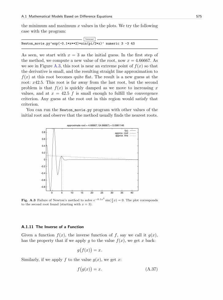
As seen, we start with x = 3 as the initial guess. In the first step ofthe method, we compute a new value of the root, now x = 4.66667. Aswe see in Figure A.3, this root is near an extreme point of f(x) so thatthe derivative is small, and the resulting straight line approximation tof(x) at this root becomes quite flat. The result is a new guess at theroot: x42.5. This root is far away from the last root, but the secondproblem is that f(x) is quickly damped as we move to increasing xvalues, and at x = 42.5 f is small enough to fulfill the convergencecriterion. Any guess at the root out in this region would satisfy thatcriterion.
You can run the Newton_movie.py program with other values of theinitial root and observe that the method usually finds the nearest roots.
Fig. A.3 Failure of Newton’s method to solve e−0.1x2sin(π
2x) = 0. The plot corresponds
to the second root found (starting with x = 3).
A.1.11 The Inverse of a Function
Given a function f(x), the inverse function of f , say we call it g(x),has the property that if we apply g to the value f(x), we get x back:
g(f(x)
)= x.
Similarly, if we apply f to the value g(x), we get x:
f(g(x)
)= x. (A.37)

576 A Sequences and Difference Equations
By hand, you substitute g(x) by (say) y in (A.37) and solve (A.37)with respect to y to find some x expression for the inverse function.For example, given f(x) = x2−1, we must solve y2−1 = x with respectto y. To ensure a unique solution for y, the x values have to be limitedto an interval where f(x) is monotone, say x ∈ [0, 1] in the presentexample. Solving for y gives y =
√1 + x, therefore g(x) =
√1 + x. It
is easy to check that f(g(x)) = (√1 + x)2 − 1 = x.
Numerically, we can use the “definition” (A.37) of the inverse func-tion g at one point at a time. Suppose we have a sequence of points x0 <x1 < · · · < xN along the x axis such that f is monotone in [x0, xN ]:f(x0) > f(x1) > · · · > f(xN ) or f(x0) < f(x1) < · · · < f(xN ). Foreach point xi, we have
f(g(xi)
)= xi.
The value g(xi) is unknown, so let us call it γ. The equation
f(γ) = xi (A.38)
can be solved be respect γ. However, (A.38) is in general nonlinear if fis a nonlinear function of x. We must then use, e.g., Newton’s methodto solve (A.38). Newton’s method works for an equation phrased as“f(x) = 0”, which in our case is f(γ) − xi = 0, i.e., we seek the rootsof the function F (γ) ≡ f(γ) − xi. Also the derivative F ′(γ) is neededin Newton’s method. For simplicity we may use an approximate finitedifference:
dF
dγ≈ F (γ + h)− F (γ − h)
2h.
As start value γ0, we can use the previously computed g value: gi−1.We introduce the short notation γ = Newton(F, γ0) to indicate thesolution of F (γ) = 0 with initial guess γ0.
The computation of all the g0, . . . , gN values can now be expressedby
gi = Newton(F, gi−1), i = 1, . . . , N, (A.39)
and for the first point we may use x0 as start value (for instance):
g0 = Newton(F, x0). (A.40)
Equations (A.39)–(A.40) constitute a difference equation for gi, sincegiven gi−1, we can compute the next element of the sequence by (A.39).Because (A.39) is a nonlinear equation in the new value gi, and (A.39)is therefore an example of a nonlinear difference equation.
The following program computes the inverse function g(x) of f(x) atsome discrete points x0, . . . , xN . Our sample function is f(x) = x2−1:
from Newton import Newtonfrom scitools.std import *
def f(x):

A.2 Programming with Sound 577
return x**2 - 1
def F(gamma):return f(gamma) - xi
def dFdx(gamma):return (F(gamma+h) - F(gamma-h))/(2*h)
h = 1E-6x = linspace(0.01, 3, 21)g = zeros(len(x))
for i in range(len(x)):xi = x[i]
# Compute start value (use last g[i-1] if possible)if i == 0:
gamma0 = x[0]else:
gamma0 = g[i-1]
gamma, n, F_value = Newton(F, gamma0, dFdx)g[i] = gamma
plot(x, f(x), ’r-’, x, g, ’b-’,title=’f1’, legend=(’original’, ’inverse’))
Note that with f(x) = x2 − 1, f ′(0) = 0, so Newton’s method di-vides by zero and breaks down unless with let x0 > 0, so here weset x0 = 0.01. The f function can easily be edited to let the programcompute the inverse of another function. The F function can remainthe same since it applies a general finite difference to approximate thederivative of the f(x) function. The complete program is found in thefile inverse_function.py. A better implementation is suggested in Ex-ercise 7.26.
A.2 Programming with Sound
Sound on a computer is nothing but a sequence of numbers. As anexample, consider the famous A tone at 440 Hz. Physically, this is anoscillation of a tuning fork, loudspeaker, string or another mechanicalmedium that makes the surrounding air also oscillate and transportthe sound as a compression wave. This wave may hit our ears andthrough complicated physiological processes be transformed to an elec-trical signal that the brain can recognize as sound. Mathematically, theoscillations are described by a sine function of time:
s(t) = A sin(2πft), (A.41)
where A is the amplitude or strength of the sound and f is the frequency(440 Hz for the A in our example). In a computer, s(t) is representedat discrete points of time. CD quality means 44100 samples per second.Other sample rates are also possible, so we introduce r as the sample

578 A Sequences and Difference Equations
rate. An f Hz tone lasting for m seconds with sample rate r can thenbe computed as the sequence
sn = A sin
(2πf
n
r
), n = 0, 1, . . . ,m · r. (A.42)
With Numerical Python this computation is straightforward and veryefficient. Introducing some more explanatory variable names than r, A,and m, we can write a function for generating a note:
import numpydef note(frequency, length, amplitude=1, sample_rate=44100):
time_points = numpy.linspace(0, length, length*sample_rate)data = numpy.sin(2*numpy.pi*frequency*time_points)data = amplitude*datareturn data
A.2.1 Writing Sound to File
The note function above generates an array of float data representinga note. The sound card in the computer cannot play these data, becausethe card assumes that the information about the oscillations appearsas a sequence of two-byte integers. With an array’s astype method wecan easily convert our data to two-byte integers instead of floats:
data = data.astype(numpy.int16)
That is, the name of the two-byte integer data type in numpy is int16
(two bytes are 16 bits). The maximum value of a two-byte integeris 215 − 1, so this is also the maximum amplitude. Assuming thatamplitude in the note function is a relative measure of intensity, suchthat the value lies between 0 and 1, we must adjust this amplitude tothe scale of two-byte integers:
max_amplitude = 2**15 - 1data = max_amplitude*data
The data array of int16 numbers can be written to a file and playedas an ordinary file in CD quality. Such a file is known as a wave fileor simply a WAV file since the extension is .wav. Python has a modulewave for creating such files. Given an array of sound, data, we have inSciTools a module sound with a function write for writing the data toa WAV file (using functionality from the wave module):
import scitools.soundscitools.sound.write(data,’Atone.wav’)
You can now use your favorite music player to play the Atone.wav file,or you can play it from within a Python program using

A.2 Programming with Sound 579
scitools.sound.play(’Atone.wav’)
The write function can take more arguments and write, e.g., a stereofile with two channels, but we do not dive into these details here.
A.2.2 Reading Sound from File
Given a sound signal in a WAV file, we can easily read this signal into anarray and mathematically manipulate the data in the array to changethe flavor of the sound, e.g., add echo, treble, or bass. The recipe forreading a WAV file with name filename is
data = scitools.sound.read(filename)
The data array has elements of type int16. Often we want to computewith this array, and then we need elements of float type, obtained bythe conversion
data = data.astype(float)
The write function automatically transforms the element type back toint16 if we have not done this explicitly.
One operation that we can easily do is adding an echo. Mathemat-ically this means that we add a damped delayed sound, where theoriginal sound has weight β and the delayed part has weight 1 − β,such that the overall amplitude is not altered. Let d be the delay inseconds. With a sampling rate r the number of indices in the delaybecomes dr, which we denote by b. Given an original sound sequencesn, the sound with echo is the sequence
en = βsn + (1− β)sn−b. (A.43)
We cannot start n at 0 since e0 = s0−b = s−b which is a value outsidethe sound data. Therefore we define en = sn for n = 0, 1, . . . , b, and addthe echo thereafter. A simple loop can do this (again we use descriptivevariable names instead of the mathematical symbols introduced):
def add_echo(data, beta=0.8, delay=0.002, sample_rate=44100):newdata = data.copy()shift = int(delay*sample_rate) # b (math symbol)for i in range(shift, len(data)):
newdata[i] = beta*data[i] + (1-beta)*data[i-shift]return newdata
The problem with this function is that it runs slowly, especially when wehave sound clips lasting several seconds (recall that for CD quality weneed 44100 numbers per second). It is therefore necessary to vectorizethe implementation of the difference equation for adding echo. Theupdate is then based on adding slices:

580 A Sequences and Difference Equations
newdata[shift:] = beta*data[shift:] + \(1-beta)*data[:len(data)-shift]
A.2.3 Playing Many Notes
How do we generate a melody mathematically in a computer program?With the note function we can generate a note with a certain amplitude,frequency, and duration. The note is represented as an array. Puttingsound arrays for different notes after each other will make up a melody.If we have several sound arrays data1, data2, data3, . . . , we can makea new array consisting of the elements in the first array followed by theelements of the next array followed by the elements in the next arrayand so forth:
data = numpy.concatenate((data1, data2, data3, ...))
Here is an example of creating a little melody (start of “NothingElse Matters” by Metallica) using constant (max) amplitude of all thenotes:
E1 = note(164.81, .5)G = note(392, .5)B = note(493.88, .5)E2 = note(659.26, .5)intro = numpy.concatenate((E1, G, B, E2, B, G))high1_long = note(987.77, 1)high1_short = note(987.77, .5)high2 = note(1046.50, .5)high3 = note(880, .5)high4_long = note(659.26, 1)high4_medium = note(659.26, .5)high4_short = note(659.26, .25)high5 = note(739.99, .25)pause_long = note(0, .5)pause_short = note(0, .25)song = numpy.concatenate((intro, intro, high1_long, pause_long, high1_long,pause_long, pause_long,high1_short, high2, high1_short, high3, high1_short,high3, high4_short, pause_short, high4_long, pause_short,high4_medium, high5, high4_short))
song *= max_amplitudescitools.sound.play(song)scitools.sound.write(song, ’tmp.wav’)
We could send song to the add_echo function to get some echo, andwe could also vary the amplitudes to get more dynamics into thesong. You can find the generation of notes above as the functionNothing_Else_Matters(echo=False) in the scitools.sound module.
A.2.4 Music of a Sequence
Problem. The purpose of this example is to listen to the sound gen-erated by two mathematical sequences. The first one is given by an

A.2 Programming with Sound 581
explicit formula, constructed to oscillate around 0 with decreasing am-plitude:
xn = e−4n/N sin(8πn/N). (A.44)
The other sequence is generated by the difference equation (A.13) forlogistic growth, repeated here for convenience:
xn = xn−1 + qxn−1(1− xn−1), x = x0. (A.45)
We let x0 = 0.01 and q = 2. This leads to fast initial growth toward thelimit 1, and then oscillations around this limit (this problem is studiedin Exercise A.23).
The absolute value of the sequence elements xn are of size between0 and 1, approximately. We want to transform these sequence elementsto tones, using the techniques of Appendix A.2. First we convert xn toa frequency the human ear can hear. The transformation
yn = 440 + 200xn (A.46)
will make a standard A reference tone out of xn = 0, and for the max-imum value of xn around 1 we get a tone of 640 Hz. Elements of thesequence generated by (A.44) lie between −1 and 1, so the correspond-ing frequencies lie between 240 Hz and 640 Hz. The task now is to makea program that can generate and play the sounds.
Solution. Tones can be generated by the note function from thescitools.sound module. We collect all tones corresponding to all theyn frequencies in a list tones. Letting N denote the number of sequenceelements, the relevant code segment reads
from scitools.sound import *freqs = 440 + x*200tones = []duration = 30.0/N # 30 sec sound in totalfor n in range(N+1):
tones.append(max_amplitude*note(freqs[n], duration, 1))data = concatenate(tones)write(data, filename)data = read(filename)play(filename)
It is illustrating to plot the sequences too,
plot(range(N+1), freqs,’ro’)
To generate the sequences (A.44) and (A.45), we make two func-tions, oscillations and logistic, respectively. These functions takethe number of sequence elements (N) as input and return the sequencestored in an array.
In another function make_sound we compute the sequence, transformthe elements to frequencies, generate tones, write the tones to file, andplay the sound file.

582 A Sequences and Difference Equations
As always, we collect the functions in a module and include a testblock where we can read the choice of sequence and the sequence lengthfrom the command line. The complete module file look as follows:
from scitools.sound import *from scitools.std import *
def oscillations(N):x = zeros(N+1)for n in range(N+1):
x[n] = exp(-4*n/float(N))*sin(8*pi*n/float(N))return x
def logistic(N):x = zeros(N+1)x[0] = 0.01q = 2for n in range(1, N+1):
x[n] = x[n-1] + q*x[n-1]*(1 - x[n-1])return x
def make_sound(N, seqtype):filename = ’tmp.wav’x = eval(seqtype)(N)# Convert x values to frequences around 440freqs = 440 + x*200plot(range(N+1), freqs, ’ro’)# Generate tonestones = []duration = 30.0/N # 30 sec sound in totalfor n in range(N+1):
tones.append(max_amplitude*note(freqs[n], duration, 1))data = concatenate(tones)write(data, filename)data = read(filename)play(filename)
if __name__ == ’__main__’:try:
seqtype = sys.argv[1]N = int(sys.argv[2])
except IndexError:print ’Usage: %s oscillations|logistic N’ % sys.argv[0]sys.exit(1)
make_sound(N, seqtype)
This code should be quite easy to read at the present stage in the book.However, there is one statement that deserves a comment:
x = eval(seqtype)(N)
The seqtype argument reflects the type of sequence and is a string thatthe user provides on the command line. The values of the string equalthe function names oscillations and logistic. With eval(seqtype)
we turn the string into a function name. For example, if seqtype is’logistic’, performing an eval(seqtype)(N) is the same as if we hadwritten logistic(N). This technique allows the user of the program tochoose a function call inside the code. Without eval we would need toexplicitly test on values:

A.3 Exercises 583
if seqtype ==’logistic’:x = logistic(N)
elif seqtype ==’oscillations’:x = oscillations(N)
This is not much extra code to write in the present example, but if wehave a large number of functions generating sequences, we can save alot of boring if-else code by using the eval construction.
The next step, as a reader who have understood the problem andthe implementation above, is to run the program for two cases: theoscillations sequence with N = 40 and the logistic sequence withN = 100. By altering the q parameter to lower values, you get othersounds, typically quite boring sounds for non-oscillating logistic growth(q < 1). You can also experiment with other transformations of theform (A.46), e.g., increasing the frequency variation from 200 to 400.
A.3 Exercises
Exercise A.1. Determine the limit of a sequence.Given the sequence
an =7 + 1/n
3− 1/n2,
make a program that computes and prints out an for n = 1, 2, . . . , N .Read N from the command line. Does an approach a finite limit whenn → ∞? Name of program file: sequence_limit1.py. �
Exercise A.2. Determine the limit of a sequence.Solve Exercise A.1 when the sequence of interest is given by
Dn =sin(2−n)
2−n.
Name of program file: sequence_limit2.py. �
Exercise A.3. Experience convergence problems.Given the sequence
Dn =f(x+ h)− f(x)
h, h = 2−n (A.47)
make a function D(f, x, N) that takes a function f(x), a value x, andthe number N of terms in the sequence as arguments, and returns anarray with the Dn values for n = 0, 1, . . . , N − 1. Make a call to the D
function with f(x) = sinx, x = 0, and N = 80. Plot the evolution ofthe computed Dn values, using small circles for the data points.
Make another call to D where x = π and plot this sequence in aseparate figure. What would be your expected limit? Why do the com-

584 A Sequences and Difference Equations
putations go wrong for large N? (Hint: Print out the numerator anddenominator in Dn.) Name of program file: sequence_limits3.py. �
Exercise A.4. Compute π via sequences.The following sequences all converge to π:
(an)∞n=1, an = 4
n∑k=1
(−1)k+1
2k − 1,
(bn)∞n=1, bn =
(6
n∑k=1
k−2
)1/2
,
(cn)∞n=1, cn =
(90
n∑k=1
k−4
)1/4
,
(dn)∞n=1, dn =
6√3
n∑k=0
(−1)k
3k(2k + 1),
(en)∞n=1, en = 16
n∑k=0
(−1)k
52k+1(2k + 1)− 4
n∑k=0
(−1)k
2392k+1(2k + 1).
Make a function for each sequence that returns an array with the el-ements in the sequence. Plot all the sequences, and find the one thatconverges fastest toward the limit π. Name of program file: pi.py. �
Exercise A.5. Reduce memory usage of difference equations.Consider the program growth_years.py from Appendix A.1.1. Since
xn depends on xn−1 only, we do not need to store all the N + 1 xnvalues. We actually only need to store xn and its previous value xn−1.Modify the program to use two variables for xn and not an array. Alsoavoid the index_set list and use an integer counter for n and a while
instead. (Of course, without the arrays it is not possible to plot thedevelopment of xn, so you have to remove the plot call.) Name ofprogram file: growth_years_efficient.py. �
Exercise A.6. Compute the development of a loan.Solve (A.16)–(A.17) for n = 1, 2, . . . , N in a Python function. Name
of program file: loan.py. �
Exercise A.7. Solve a system of difference equations.Solve (A.32)–(A.33) by generating the xn and cn sequences in
a Python function. Let the function return the computed se-quences as arrays. Plot the xn sequence. Name of program file:fortune_and_inflation1.py. �
Exercise A.8. Extend the model (A.32)–(A.33).In the model (A.32)–(A.33) the new fortune is the old one, plus the
interest, minus the consumption. During year n, xn is normally also

A.3 Exercises 585
reduced with t percent tax on the earnings xn−1 − xn−2 in year n− 1.Extend the model with an appropriate tax term, modify the programfrom Exercise A.7, and plot xn with tax (t = 28) and without tax(t = 0). Name of program file: fortune_and_inflation2.py. �
Exercise A.9. Experiment with the program from Exer. A.8.Suppose you expect to live for N years and can accept that the for-
tune xn vanishes after N years. Experiment with the program fromExercise A.8 for how large the initial c0 can be in this case. Choosesome appropriate values for p, q, I, and t. Name of program file:fortune_and_inflation3.py. �
Exercise A.10. Change index in a difference equation.A mathematically equivalent equation to (A.5) is
xi+1 = xi +p
100xi, (A.48)
since the name of the index can be chosen arbitrarily. Suppose someonehas made the following program for solving (A.48) by a slight editingof the program growth1.py:
from scitools.std import *x0 = 100 # initial amountp = 5 # interest rateN = 4 # number of yearsindex_set = range(N+1)x = zeros(len(index_set))
# Compute solutionx[0] = x0for i in index_set[1:]:
x[i+1] = x[i] + (p/100.0)*x[i]print xplot(index_set, x, ’ro’, xlabel=’years’, ylabel=’amount’)
This program does not work. Make a correct version, but keep thedifference equations in its present form with the indices i+1 and i.Name of program file: growth1_index_ip1.py. �
Exercise A.11. Construct time points from dates.A certain quantity p (which may be an interest rate) is piecewise
constant and undergoes changes at some specific dates, e.g.,
p changes to
⎧⎪⎪⎪⎪⎪⎪⎨⎪⎪⎪⎪⎪⎪⎩
4.5 on Jan 4, 20094.75 on March 21, 20096.0 on April 1, 20095.0 on June 30, 20094.5 on Nov 1, 20092.0 on April 1, 2010
(A.49)
Given a start date d1 and an end date d2, fill an array p with the rightp values, where the array index counts days. Use the datetime module

586 A Sequences and Difference Equations
to compute the number of days between dates. Name of program file:dates2days.py. �Exercise A.12. Solve nonlinear equations by Newton’s method.
Import the Newton function from the Newton.py file from Ap-pendix A.1.10 to solve the following nonlinear algebraic equations:
sinx = 0, (A.50)
x = sinx, (A.51)
x5 = sinx, (A.52)
x4 sinx = 0, (A.53)
x4 = 0, (A.54)
x10 = 0, (A.55)
tanhx = x10. (A.56)
Implement the f(x) and f ′(x) functions, required by Newton’s method,for each of the nonlinear equations. Collect the names of the f(x) andf ′(x) in a list, and make a for loop over this list to call the Newton
function for each equation. Read the starting point x0 from the com-mand line. Print out the evolution of the roots (based on the info list)for each equation. You will need to carefully plot the various f(x) func-tions to understand how Newton’s method will behave in each case fordifferent starting values. Find a starting value x0 value for each equa-tion so that Newton’s method will converge toward the root x = 0.Name of program file: Newton_examples.py. �Exercise A.13. Visualize the convergence of Newton’s method.
Let x0, x1, . . . , xN be the sequence of roots generated by New-ton’s method applied to a nonlinear algebraic equation f(x) =0 (cf. Appendix A.1.10). In this exercise, the purpose is to plotthe sequences (xn)
Nn=0 and (|f(xn)|)Nn=0. Make a general function
Newton_plot(f, x, dfdx, epsilon=1E-7) for this purpose. The argu-ments f and dfdx are Python functions representing the f(x) functionin the equation and its derivative f ′(x), respectively. Newton’s methodis run until |f(xN )| ≤ ε, and the ε value is stored in the epsilon ar-gument. The Newton_plot function should make two separate plots of(xn)
Nn=0 and (|f(xn)|)Nn=0 on the screen and also save these plots to
PNG files. Because of the potentially wide scale of values that |f(xn)|may exhibit, it may be wise to use a logarithmic scale on the y axis.(Hint: You can save quite some coding by calling the improved Newton
function from Appendix A.1.10, which is available in the Newtonmodulein src/diffeq/Newton.py.)
Demonstrate the function on the equation x6 sinπx = 0, withε = 10−13. Try different starting values for Newton’s method: x0 =−2.6,−1.2, 1.5, 1.7, 0.6. Compare the results with the exact solutionsx = . . . ,−2− 1, 0, 1, 2, . . . . Name of program file: Newton2.py. �

A.3 Exercises 587
Exercise A.14. Implement the Secant method.Newton’s method (A.34) for solving f(x) = 0 requires the derivative
of the function f(x). Sometimes this is difficult or inconvenient. Thederivative can be approximated using the last two approximations tothe root, xn−2 and xn−1:
f ′(xn−1) ≈f(xn−1)− f(xn−2)
xn−1 − xn−2.
Using this approximation in (A.34) leads to the Secant method:
xn = xn−1 −f(xn−1)(xn−1 − xn−2)
f(xn−1)− f(xn−2), x0, x1 given. (A.57)
Here n = 2, 3, . . . . Make a program that applies the Secant method tosolve x5 = sinx. Name of program file: Secant.py. �
Exercise A.15. Test different methods for root finding.Make a program for solving f(x) = 0 by Newton’s method (Ap-
pendix A.1.10), the Bisection method (Chapter 4.6.2), and the Secantmethod (Exercise A.14). For each method, the sequence of root ap-proximations should be written out (nicely formatted) on the screen.Read f(x), f ′(x), a, b, x0, and x1 from the command line. Newton’smethod starts with x0, the Bisection method starts with the interval[a, b], whereas the Secant method starts with x0 and x1.
Run the program for each of the equations listed in Exercise A.12.You should first plot the f(x) functions as suggested in that exercise soyou know how to choose x0, x1, a, and b in each case. Name of programfile: root_finder_examples.py. �
Exercise A.16. Make difference equations for the Midpoint rule.Use the ideas of Appendix A.1.7 to make a similar system of
difference equations and corresponding implementation for the Mid-point integration rule from Exercise 3.8. Name of program file:diffeq_midpoint.py. �
Exercise A.17. Compute the arc length of a curve.Sometimes one wants to measure the length of a curve y = f(x) for
x ∈ [a, b]. The arc length from f(a) to some point f(x) is denoted bys(x) and defined through an integral
s(x) =
∫ x
a
√1 +
[f ′(ξ)
]2dξ. (A.58)
We can compute s(x) via difference equations as explained in Ap-pendix A.1.7. Make a Python function arclength(f, a, b, n) that re-turns an array s with s(x) values for n uniformly spaced coordinates xin [a, b]. Here f(x) is the Python implementation of the function that

588 A Sequences and Difference Equations
defines the curve we want to compute the arc length of. How can youtest that the arclength function works correctly? Test the function on
f(x) =
∫ x
−2=
1√2π
e−4t2dt, x ∈ [−2, 2].
Compute f(x) and plot it together with s(x). Name of program file:arclength.py. �
Exercise A.18. Find difference equations for computing sinx.The purpose of this exercise is to derive and implement difference
equations for computing a Taylor polynomial approximation to sinx,using the same ideas as in (A.24)–(A.25) for a Taylor polynomial ap-proximation to ex in Appendix A.1.8.
The Taylor series for sinx is presented in Exercise 5.21, Equa-tion (5.21) on page 248. To compute S(x;n) efficiently, we try to com-pute a new term from the last computed term. Let S(x;n) =
∑nj=0 aj ,
where the expression for a term aj follows from the formula (5.21). De-rive the following relation between two consecutive terms in the series,
aj = − x2
(2j + 1)2jaj−1. (A.59)
Introduce sj = S(x; j − 1) and define s0 = 0. We use sj to accumulateterms in the sum. For the first term we have a0 = x. Formulate a systemof two difference equations for sj and aj in the spirit of (A.24)–(A.25).Implement this system in a function sine_Taylor(x, n), which returnssn+1 and |an+1|. The latter is the first neglected term in the sum (sincesn+1 =
∑nj=0 aj) and may act as a rough measure of the size of the
error in the approximation.Verify the implementation by computing the difference equations
for n = 2 by hand (or in a separate program) and comparing withthe output from the sine_Taylor function. Also make a table of sn forvarious x and n values to verify that the accuracy of a Taylor poly-nomial improves as n increases and x decreases. Be aware of the factthat sine_Taylor(x, n) can give extremely inaccurate approximationsto sinx if x is not sufficiently small and n sufficiently large. Name ofprogram file: sin_Taylor_series_diffeq.py. �
Exercise A.19. Find difference equations for computing cosx.Carry out the steps in Exercise A.18, but do it for the Taylor se-
ries of cosx instead of sinx (look up the Taylor series for cosx in amathematics textbook or search on the Internet). Name of programfile: cos_Taylor_series_diffeq.py. �
Exercise A.20. Make a guitar-like sound.Given start values x0, x1, . . . , xp, the following difference equation is
known to create guitar-like sound:
A.3 Exercises 589
xn =1
2(xn−p + xn−p−1), n = p+ 1, . . . , N. (A.60)
With a sampling rate r, the frequency of this sound is given by r/p.Make a program with a function solve(x, p) which returns the solu-tion array x of (A.60). To initialize the array x[0:p+1] we look at twomethods, which can be implemented in two alternative functions:
1. x0 = 1, x1 = x2 = · · · = xp = 02. x0, . . . , xp are uniformly distributed random numbers in [−1, 1]
Import max_amplitude, write, and play from the scitools.sound mod-ule. Choose a sampling rate r and set p = r/440 to create a 440 Hz tone(A). Create an array x1 of zeros with length 3r such that the tone willlast for 3 seconds. Initialize x1 according to method 1 above and solve(A.60). Multiply the x1 array by max_amplitude. Repeat this processfor an array x2 of length 2r, but use method 2 for the initial valuesand choose p such that the tone is 392 Hz (G). Concatenate x1 and x2,call write and then play to play the sound. As you will experience, thissound is amazingly similar to the sound of a guitar string, first playingA for 3 seconds and then playing G for 2 seconds. (The method (A.60)is called the Karplus-Strong algorithm and was discovered in 1979 by aresearcher, Kevin Karplus, and his student Alexander Strong, at Stan-ford University.) Name of program file: guitar_sound.py. �
Exercise A.21. Damp the bass in a sound file.Given a sequence x0, . . . , xN−1, the following filter transforms the
sequence to a new sequence y0, . . . , yN−1:
yn =
⎧⎨⎩
xn, n = 0−1
4(xn−1 − 2xn + xn+1), 1 ≤ n ≤ N − 2xn, n = N − 1
(A.61)
If xn represents sound, yn is the same sound but with the bass damped.Load some sound file (e.g., the one from Exercise A.20) or call
x = scitools.sound.Nothing_Else_Matters(echo=True)
to get a sound sequence. Apply the filter (A.61) and play the result-ing sound. Plot the first 300 values in the xn and yn signals to seegraphically what the filter does with the signal. Name of program file:damp_bass.py. �
Exercise A.22. Damp the treble in a sound file.Solve Exercise A.21 to get some experience with coding a filter and
trying it out on a sound. The purpose of this exercise is to explore someother filters that reduce the treble instead of the bass. Smoothing thesound signal will in general damp the treble, and smoothing is typicallyobtained by letting the values in the new filtered sound sequence be anaverage of the neighboring values in the original sequence.

590 A Sequences and Difference Equations
The simplest smoothing filter can apply a standard average of threeneighboring values:
yn =
⎧⎨⎩
xn, n = 013(xn−1 + xn + xn+1), 1 ≤ n ≤ N − 2xn, n = N − 1
(A.62)
Two other filters put less emphasis on the surrounding values:
yn =
⎧⎨⎩
xn, n = 014(xn−1 + 2xn + xn+1), 1 ≤ n ≤ N − 2xn, n = N − 1
(A.63)
yn =
⎧⎨⎩
xn, n = 0, 1116(xn−2 + 4xn−1 + 6xn + 4xn+1 + xn+2), 2 ≤ n ≤ N − 3xn, n = N − 2, N − 1
(A.64)Apply all these three filters to a sound file and listen to the result.Plot the first 300 values in the xn and yn signals for each of the threefilters to see graphically what the filter does with the signal. Name ofprogram file: damp_treble.py. �
Exercise A.23. Demonstrate oscillatory solutions of (A.13).Modify the growth_logistic.py program from Appendix A.1.5 to
solve the equation (A.13) on page 566. Read the input parameters y0,q, and N from the command line.
Equation (A.13) has the solution yn = 1 as n → ∞. Demonstrate,by running the program, that this is the case when y0 = 0.3, q = 1,and N = 50.
For larger q values, yn does not approach a constant limit, but ynoscillates instead around the limiting value. Such oscillations are some-times observed in wildlife populations. Demonstrate oscillatory solu-tions when q is changed to 2 and 3.
It could happen that yn stabilizes at a constant level for larger N .Demonstrate that this is not the case by running the program withN = 1000. Name of program file: growth_logistic2.py. �
Exercise A.24. Improve the program from Exer. A.23.It is tedious to run a program like the one from Exercise A.23 re-
peatedly for a wide range of input parameters. A better approach isto let the computer do the manual work. Modify the program fromExercise A.23 such that the computation of yn and the plot is madein a function. Let the title in the plot contain the parameters y0 and q(N is easily visible from the x axis). Also let the name of the plot filereflect the values of y0, q, and N . Then make loops over y0 and q toperform the following more comprehensive set of experiments:
• y0 = 0.01, 0.3

A.3 Exercises 591
• q = 0.1, 1, 1.5, 1.8, 2, 2.5, 3• N = 50
How does the initial condition (the value y0) seem to influence thesolution?
The keyword argument show=False can be used in the plot call ifyou do not want all the plot windows to appear on the screen. Nameof program file: growth_logistic3.py. �
Exercise A.25. Generate an HTML report.Extend the program made in Exercise A.24 with a report containing
all the plots. The report can be written in HTML and displayed by aweb browser. The plots must then be generated in PNG format. Thesource of the HTML file will typically look as follows:
<html><body><p><img src="tmp_y0_0.01_q_0.1_N_50.png"><p><img src="tmp_y0_0.01_q_1_N_50.png"><p><img src="tmp_y0_0.01_q_1.5_N_50.png"><p><img src="tmp_y0_0.01_q_1.8_N_50.png">...<p><img src="tmp_y0_0.01_q_3_N_1000.png"></html></body>
Let the program write out the HTML text, either to the screen or to afile (cf. Chapter 6.5). When writing to the screen, redirect the outputto a file,
Terminal
growth_logistic4.py > report.html
The file report.html can be loaded into a web browser.You may let the function making the plots return the name of the
plotfile such that this string can be inserted in the HTML file. Nameof program file: growth_logistic4.py. �
Exercise A.26. Simulate the price of wheat.The demand for wheat in year t is given by
Dt = apt + b,
where a < 0, > 0, and pt is the price of wheat. Let the supply of wheatbe
St = Apt−1 +B + ln(1 + pt−1),
where A and B are given constants. We assume that the price pt adjustssuch that all the produced wheat is sold. That is, Dt = St.
For A = 1, a = −3, b = 5, B = 0, find from numerical computations,a stable price such that the production of wheat from year to year isconstant. That is, find p such that ap+ b = Ap+B + ln(1 + p).
Assume that in a very dry year the production of wheat is much lessthan planned. Given that price this year, p0, is 4.5 and Dt = St, com-

592 A Sequences and Difference Equations
pute in a program how the prices p1, p2, . . . , pN develop. This impliessolving the difference equation
apt + b = Apt−1 +B + ln(1 + pt−1).
From the pt values, compute St and plot the points (pt, St) for t =0, 1, 2, . . . , N . How do the prices move when N → ∞? Name of programfile: wheat.py. �

Introduction to Discrete Calculus B
This Appendix is Authored by Aslak Tveito
In this chapter we will discuss how to differentiate and integrate func-tions on a computer. To do that, we have to care about how to treatmathematical functions on a computer. Handling mathematical func-tions on computers is not entirely straightforward: A function f(x)contains and infinite amount of information (function values at an in-finite number of x values on an interval), while the computer can onlystore a finite1 amount of data. Think about the cosx function. Thereare typically two ways we can work with this function on a computer.One way is to run an algorithm, like that in Exercise 3.30 on page 130,or we simply call math.cos(x) (which runs a similar type of algorithm),to compute an approximation to cosx for a given x, using a finite num-ber of calculations. The other way is to store cosx values in a table for afinite number of x values2 and use the table in a smart way to computecosx values. This latter way, known as a discrete representation of afunction, is in focus in the present chapter. With a discrete functionrepresentation, we can easily integrate and differentiate the functiontoo. Read on to see how we can do that.
The folder src/discalc contains all the program example files re-ferred to in this chapter.
B.1 Discrete Functions
Physical quantities, such as temperature, density, and velocity, are usu-ally defined as continuous functions of space and time. However, as
1 Allow yourself a moment or two to think about the terms “finite” and “infinite”; infinityis not an easy term, but it is not infinitely difficult. Or is it?2 Of course, we need to run an algorithm to populate the table with cos x numbers.
H.P. Langtangen, A Primer on Scientific Programming with Python,Texts in Computational Science and Engineering 6,
DOI 10.1007/978-3-642-30293-0, c© Springer-Verlag Berlin Heidelberg 2012
593

594 B Introduction to Discrete Calculus
mentioned in above, discrete versions of the functions are more conve-nient on computers. We will illustrate the concept of discrete functionsthrough some introductory examples. In fact, we used discrete functionsin Chapter 5 to plot curves: We defined a finite set of coordinates x andstored the corresponding function values f(x) in an array. A plottingprogram would then draw straight lines between the function values.A discrete representation of a continuous function is, from a program-ming point of view, nothing but storing a finite set of coordinates andfunction values in an array. Nevertheless, we will in this chapter bemore formal and describe discrete functions by precise mathematicalterms.
B.1.1 The Sine Function
Suppose we want to generate a plot of the sine function for values ofx between 0 and π. To this end, we define a set of x-values and anassociated set of values of the sine function. More precisely, we definen+ 1 points by
xi = ih for i = 0, 1, . . . , n (B.1)
where h = π/n and n � 1 is an integer. The associated function valuesare defined as
si = sin(xi) for i = 0, 1, . . . , n. (B.2)
Mathematically, we have a sequence of coordinates (xi)ni=0 and of func-
tion values (si)ni=0 (see the start of Appendix A for an explanation of
the notation and the sequence concept). Often we “merge” the two se-quences to one sequence of points: (xi, si)
ni=0. Sometimes we also use
a shorter notation, just xi, si, or (xi, si) if the exact limits are not ofimportance. The set of coordinates (xi)
ni=0 constitutes a mesh or a
grid. The individual coordinates xi are known as nodes in the mesh(or grid). The discrete representation of the sine function on [0, π] con-sists of the mesh and the corresponding sequence of function values(si)
ni=0 at the nodes. The parameter n is often referred to as the mesh
resolution.In a program, we represent the mesh by a coordinate array, say x, and
the function values by another array, say s. To plot the sine functionwe can simply write
from scitools.std import *
n = int(sys.argv[1])
x = linspace(0, pi, n+1)s = sin(x)plot(x, s, legend=’sin(x), n=%d’ % n, hardcopy=’tmp.eps’)
Figure B.1 shows the resulting plot for n = 5, 10, 20 and 100. Aspointed out in Chapter 5, the curve looks smoother the more points

B.1 Discrete Functions 595
we use, and since sin(x) is a smooth function, the plots in Figures B.1aand B.1b do not look sufficiently good. However, we can with our eyeshardly distinguish the plot with 100 points from the one with 20 points,so 20 points seem sufficient in this example.
Fig. B.1 Plots of sin(x) with various n.
There are no tests on the validity of the input data (n) in the previousprogram. A program including these tests reads3:
#!/usr/bin/env pythonfrom scitools.std import *
try:n = int(sys.argv[1])
except:print "usage: %s n" %sys.argv[0]sys.exit(1)
x = linspace(0, pi, n+1)s = sin(x)plot(x, s, legend=’sin(x), n=%d’ % n, hardcopy=’tmp.eps’)
Such tests are important parts of a good programming philosophy.However, for the programs displayed in this and the next chapter, weskip such tests in order to make the programs more compact and read-able as part of the rest of the text and to enable focus on the mathe-matics in the programs. In the versions of these programs in the files
3 For an explanation of the first line of this program, see Appendix H.1.

596 B Introduction to Discrete Calculus
that can be downloaded you will, hopefully, always find a test on inputdata.
B.1.2 Interpolation
Suppose we have a discrete representation of the sine function:(xi, si)
ni=0. At the nodes we have the exact sine values si, but what
about the points in between these nodes? Finding function values be-tween the nodes is called interpolation, or we can say that we interpolatea discrete function.
A graphical interpolation procedure could be to look at one of theplots in Figure B.1 to find the function value corresponding to a pointx between the nodes. Since the plot is a straight line from node valueto node value, this means that a function value between two nodes isfound from a straight line approximation4 to the underlying continuousfunction. We formulate this procedure precisely in terms of mathemat-ics in the next paragraph.
Assume that we know that a given x∗ lies in the interval from x = xkto xk+1, where the integer k is given. In the interval xk � x < xk+1, wedefine the linear function that passes through (xk, sk) and (xk+1, sk+1):
Sk(x) = sk +sk+1 − skxk+1 − xk
(x− xk). (B.3)
That is, Sk(x) coincides with sin(x) at xk and xk+1, and between thesenodes, Sk(x) is linear. We say that Sk(x) interpolates the discrete func-tion (xi, si)
ni=0 on the interval [xk, xk+1].
B.1.3 Evaluating the Approximation
Given the values (xi, si)ni=0 and the formula (B.3), we want to compute
an approximation of the sine function for any x in the interval fromx = 0 to x = π. In order to do that, we have to compute k for a givenvalue of x. More precisely, for a given x we have to find k such thatxk � x � xk+1. We can do that by defining
k = x/h�
where the function z� denotes the largest integer that is smaller than z.In Python, z� is computed by int(z). The program below takes x andn as input and computes the approximation of sin(x). The program
4 Strictly speaking, we also assume that the function to be interpolated is rather smooth.
It is easy to see that if the function is very wild, i.e., the values of the function changes veryrapidly, this procedure may fail even for very large values of n. Chapter 5.4.2 provides an
example.

B.1 Discrete Functions 597
prints the approximation S(x) and the exact5 value of sin(x) so we canlook at the development of the error when n is increased.
from numpy import *import sys
xp = eval(sys.argv[1])n = int(sys.argv[2])
def S_k(k):return s[k] + \
((s[k+1] - s[k])/(x[k+1] - x[k]))*(xp - x[k])h = pi/nx = linspace(0, pi, n+1)s = sin(x)k = int(xp/h)
print ’Approximation of sin(%s): ’ % xp, S_k(k)print ’Exact value of sin(%s): ’ % xp, sin(xp)print ’Eror in approximation: ’, sin(xp) - S_k(k)
To study the approximation, we put x =√2 and use the program
eval_sine.py for n = 5, 10 and 20.
Terminal
eval_sine.py’sqrt(2)’ 5Approximation of sin(1.41421356237): 0.951056516295Exact value of sin(1.41421356237): 0.987765945993Eror in approximation: 0.0367094296976
Terminal
eval_sine.py’sqrt(2)’ 10Approximation of sin(1.41421356237): 0.975605666221Exact value of sin(1.41421356237): 0.987765945993Eror in approximation: 0.0121602797718
Terminal
eval_sine.py’sqrt(2)’ 20Approximation of sin(1.41421356237): 0.987727284363Exact value of sin(1.41421356237): 0.987765945993Eror in approximation: 3.86616296923e-05
Note that the error is reduced as the n increases.
B.1.4 Generalization
In general, we can create a discrete version of a continuous function asfollows. Suppose a continuous function f(x) is defined on an interval
5 The value is not really exact – it is the value of sin(x) provided by the computer,math.sin(x), and this value is calculated from an algorithm that only yields an approxi-
mation to sin(x). Exercise 3.30 provides an example of the type of algorithm in question.
598 B Introduction to Discrete Calculus
ranging from x = a to x = b, and let n � 1, be a given integer. Definethe distance between nodes,
h =b− a
n,
and the nodesxi = a+ ih for i = 0, 1, . . . , n. (B.4)
The discrete function values are given by
yi = f(xi) for i = 0, 1, . . . , n. (B.5)
Now, (xi, yi)ni=0 is the discrete version of the continuous function f(x).
The program discrete_func.py takes f, a, b and n as input, computesthe discrete version of f , and then applies the discrete version to makea plot of f .
def discrete_func(f, a, b, n):x = linspace(a, b, n+1)y = zeros(len(x))for i in xrange(len(x)):
y[i] = func(x[i])return x, y
from scitools.std import *
f_formula = sys.argv[1]a = eval(sys.argv[2])b = eval(sys.argv[3])n = int(sys.argv[4])f = StringFunction(f_formula)
x, y = discrete_func(f, a, b, n)plot(x, y)
We can equally well make a vectorized version of the discrete_func
function:
def discrete_func(f, a, b, n):x = linspace(a, b, n+1)y = f(x)return x, y
However, for the StringFunction tool to work properly in vectorizedmode, we need to follow the recipe in Chapter 5.5.1:
f = StringFunction(f_formula)f.vectorize(globals())
The corresponding vectorized program is found in the filediscrete_func_vec.py.

B.2 Differentiation Becomes Finite Differences 599
B.2 Differentiation Becomes Finite Differences
You have heard about derivatives. Probably, the following formulas arewell known to you:
d
dxsin(x) = cos(x),
d
dxln(x) =
1
x,
d
dxxm = mxm−1.
But why is differentiation so important? The reason is quite simple:The derivative is a mathematical expression of change. And change is,of course, essential in modeling various phenomena. If we know thestate of a system, and we know the laws of change, then we can, inprinciple, compute the future of that system. Appendix C treats thistopic in detail. Appendix A also computes the future of systems, basedon modeling changes, but without using differentiation. In Appendix Cyou will see that reducing the step size in the difference equations inAppendix A results in derivatives instead of pure differences. However,differentiation of continuous functions is somewhat hard on a computer,so we often end up replacing the derivatives by differences. This ideais quite general, and every time we use a discrete representation of afunction, differentiation becomes differences, or finite differences as weusually say.
The mathematical definition of differentiation reads
f ′(x) = limε→0
f(x+ ε)− f(x)
ε.
You have probably seen this definition many times, but have you under-stood what it means and do you think the formula has a great practicalvalue? Although the definition requires that we pass to the limit, weobtain quite good approximations of the derivative by using a fixedpositive value of ε. More precisely, for a small ε > 0, we have
f ′(x) ≈ f(x+ ε)− f(x)
ε.
The fraction on the right-hand side is a finite difference approximationto the derivative of f at the point x. Instead of using ε it is morecommon to introduce h = ε in finite differences, i.e., we like to write
f ′(x) ≈ f(x+ h)− f(x)
h. (B.6)
600 B Introduction to Discrete Calculus
B.2.1 Differentiating the Sine Function
In order to get a feeling for how good the approximation (B.6) to thederivative really is, we explore an example. Consider f(x) = sin(x) andthe associated derivative f ′(x) = cos(x). If we put x = 1, we have
f ′(1) = cos(1) ≈ 0.540,
and by putting h = 1/100 in (B.6) we get
f ′(1) ≈ f(1 + 1/100)− f(1)
1/100=
sin(1.01)− sin(1)
0.01≈ 0.536.
The program forward_diff.py, shown below, computes the deriva-tive of f(x) using the approximation (B.6), where x and h are inputparameters.
def diff(f, x, h):return (f(x+h) - f(x))/float(h)
from math import *import sys
x = eval(sys.argv[1])h = eval(sys.argv[2])
approx_deriv = diff(sin, x, h)exact = cos(x)print ’The approximated value is: ’, approx_derivprint ’The correct value is: ’, exactprint ’The error is: ’, exact - approx_deriv
Running the program for x = 1 and h = 1/1000 gives
Terminal
forward_diff.py 1 0.001The approximated value is: 0.53988148036The correct value is: 0.540302305868The error is: 0.000420825507813
B.2.2 Differences on a Mesh
Frequently, we will need finite difference approximations to a discretefunction defined on a mesh. Suppose we have a discrete representationof the sine function: (xi, si)
ni=0, as introduced in Chapter B.1.1. We want
to use (B.6) to compute approximations to the derivative of the sinefunction at the nodes in the mesh. Since we only have function valuesat the nodes, the h in (B.6) must be the difference between nodes, i.e.,h = xi+1−xi. At node xi we then have the following approximation ofthe derivative:
zi =si+1 − si
h, (B.7)

B.2 Differentiation Becomes Finite Differences 601
for i = 0, 1, . . . , n − 1. Note that we have not defined an approximatederivative at the end point x = xn. We cannot apply (B.7) directlysince sn+1 is undefined (outside the mesh). However, the derivative ofa function can also be defined as
f ′(x) = limε→0
f(x)− f(x− ε)
ε,
which motivates the following approximation for a given h > 0,
f ′(x) ≈ f(x)− f(x− h)
h. (B.8)
This alternative approximation to the derivative is referred to as abackward difference formula, whereas the expression (B.6) is knownas a forward difference formula. The names are natural: The forwardformula goes forward, i.e., in the direction of increasing x and i to col-lect information about the change of the function, while the backwardformula goes backwards, i.e., toward smaller x and i value to fetchfunction information.
At the end point we can apply the backward formula and thus define
zn =sn − sn−1
h. (B.9)
We now have an approximation to the derivative at all the nodes.A plain specialized program for computing the derivative of thesine function on a mesh and comparing this discrete derivative withthe exact derivative is displayed below (the name of the file isdiff_sine_plot1.py).
from scitools.std import *
n = int(sys.argv[1])
h = pi/nx = linspace(0, pi, n+1)s = sin(x)z = zeros(len(s))for i in xrange(len(z)-1):
z[i] = (s[i+1] - s[i])/h# Special formula for end point_z[-1] = (s[-1] - s[-2])/hplot(x, z)
xfine = linspace(0, pi, 1001) # for more accurate plotexact = cos(xfine)hold()plot(xfine, exact)legend(’Approximate function’,’Correct function’)title(’Approximate and discrete functions, n=%d’ % n)
In Figure B.2 we see the resulting graphs for n = 5, 10, 20 and 100.Again, we note that the error is reduced as n increases.

602 B Introduction to Discrete Calculus
Fig. B.2 Plots for exact and approximate derivatives of sin(x) with varying values of theresolution n.
B.2.3 Generalization
The discrete version of a continuous function f(x) defined on an interval[a, b] is given by (xi, yi)
ni=0 where
xi = a+ ih,
andyi = f(xi)
for i = 0, 1, . . . , n. Here, n � 1 is a given integer, and the spacingbetween the nodes is given by
h =b− a
n.
A discrete approximation of the derivative of f is given by (xi, zi)ni=0
where
zi =yi+1 − yi
h
i = 0, 1, . . . , n− 1, and
zn =yn − yn−1
h.

B.3 Integration Becomes Summation 603
The collection (xi, zi)ni=0 is the discrete derivative of the discrete version
(xi, fi)ni=0 of the continuous function f(x). The program below, found
in the file diff_func.py, takes f, a, b and n as input and computes thediscrete derivative of f on the mesh implied by a, b, and h, and then aplot of f and the discrete derivative is made.
def diff(f, a, b, n):x = linspace(a, b, n+1)y = zeros(len(x))z = zeros(len(x))h = (b-a)/float(n)for i in xrange(len(x)):
y[i] = func(x[i])for i in xrange(len(x)-1):
z[i] = (y[i+1] - y[i])/hz[n] = (y[n] - y[n-1])/hreturn y, z
from scitools.std import *f_formula = sys.argv[1]a = eval(sys.argv[2])b = eval(sys.argv[3])n = int(sys.argv[4])
f = StringFunction(f_formula)y, z = diff(f, a, b, n)plot(x, y, ’r-’, x, z, ’b-’,
legend=(’function’, ’derivative’))
B.3 Integration Becomes Summation
Some functions can be integrated analytically. You may remember6 thefollowing cases, ∫
xmdx =1
m+ 1xm+1 for m �= −1,
∫sin(x)dx = − cos(x),
∫x
1 + x2dx =
1
2ln(x2 + 1
).
These are examples of so-called indefinite integrals. If the function canbe integrated analytically, it is straightforward to evaluate an associ-ated definite integral. For example, we have7
6 Actually, we congratulate you if you remember the third one!7 Recall, in general, that [
f(x)]ba= f(b)− f(a).

604 B Introduction to Discrete Calculus
∫ 1
0xmdx =
[1
m+ 1xm+1
]10
=1
m+ 1,
∫ π
0sin(x)dx =
[− cos(x)
]π0= 2,
∫ 1
0
x
1 + x2dx =
[1
2ln(x2 + 1
)]10
=1
2ln 2.
But lots of functions cannot be integrated analytically and thereforedefinite integrals must be computed using some sort of numerical ap-proximation. Above, we introduced the discrete version of a function,and we will now use this construction to compute an approximation ofa definite integral.
B.3.1 Dividing into Subintervals
Let us start by considering the problem of computing the integral ofsin(x) from x = 0 to x = π. This is not the most exciting or challengingmathematical problem you can think of, but it is good practice to startwith a problem you know well when you want to learn a new method.In Chapter B.1.1 we introduce a discrete function (xi, si)
ni=0 where
h = π/n, si = sin(xi) and xi = ih for i = 0, 1, . . . , n. Furthermore, inthe interval xk � x < xk+1, we defined the linear function
Sk(x) = sk +sk+1 − skxk+1 − xk
(x− xk).
We want to compute an approximation of the integral of the functionsin(x) from x = 0 to x = π. The integral
∫ π
0sin(x)dx
can be divided into subintegrals defined on the intervals xk � x < xk+1,leading to the following sum of integrals:
∫ π
0sin(x)dx =
n−1∑k=0
∫ xk+1
xk
sin(x)dx.
To get a feeling for this split of the integral, let us spell the sum out inthe case of only four subintervals. Then n = 4, h = π/4,
x0 = 0,
x1 = π/4,
x2 = π/2,
B.3 Integration Becomes Summation 605
x3 = 3π/4
x4 = π.
The interval from 0 to π is divided into four intervals of equal length,and we can divide the integral similarly,
∫ π
0sin(x)dx =
∫ x1
x0
sin(x)dx+
∫ x2
x1
sin(x)dx
+
∫ x3
x2
sin(x)dx+
∫ x4
x3
sin(x)dx. (B.10)
So far we have changed nothing – the integral can be split in this way– with no approximation at all. But we have reduced the problem ofapproximating the integral
∫ π
0sin(x)dx
down to approximating integrals on the subintervals, i.e. we need ap-proximations of all the following integrals
∫ x1
x0
sin(x)dx,
∫ x2
x1
sin(x)dx,
∫ x3
x2
sin(x)dx,
∫ x4
x3
sin(x)dx.
The idea is that the function to be integrated changes less over thesubintervals than over the whole domain [0, π] and it might be rea-sonable to approximate the sine by a straight line, Sk(x), over eachsubinterval. The integration over a subinterval will then be very easy.
B.3.2 Integration on Subintervals
The task now is to approximate integrals on the form∫ xk+1
xk
sin(x)dx.
Sincesin(x) ≈ Sk(x)
on the interval (xk, xk+1), we have
∫ xk+1
xk
sin(x)dx ≈∫ xk+1
xk
Sk(x)dx.
In Figure B.3 we have graphed Sk(x) and sin(x) on the interval(xk, xk+1) for k = 1 in the case of n = 4. We note that the integral ofS1(x) on this interval equals the area of a trapezoid, and thus we have

606 B Introduction to Discrete Calculus
Fig. B.3 Sk(x) and sin(x) on the interval (xk, xk+1) for k = 1 and n = 4.
∫ x2
x1
S1(x)dx =1
2
(S1(x2) + S1(x1)
)(x2 − x1),
so ∫ x2
x1
S1(x)dx =h
2(s2 + s1),
and in general we have∫ xk+1
xk
sin(x)dx ≈ 1
2(sk+1 + sk)(xk+1 − xk)
=h
2(sk+1 + sk).
B.3.3 Adding the Subintervals
By adding the contributions from each subinterval, we get
∫ π
0sin(x)dx =
n−1∑k=0
∫ xk+1
xk
sin(x)dx
≈n−1∑k=0
h
2(sk+1 + sk),
so ∫ π
0sin(x)dx ≈ h
2
n−1∑k=0
(sk+1 + sk). (B.11)
In the case of n = 4, we have

B.3 Integration Becomes Summation 607
∫ π
0sin(x)dx ≈ h
2
[(s1 + s0) + (s2 + s1) + (s3 + s2) + (s4 + s3)
]
=h
2
[s0 + 2(s1+s2+s3) + s4
].
One can show that (B.11) can be alternatively expressed as8
∫ π
0sin(x)dx ≈ h
2
[s0 + 2
n−1∑k=1
sk + sn
]. (B.12)
This approximation formula is referred to as the Trapezoidal rule ofnumerical integration. Using the more general program trapezoidal.py,presented in the next section, on integrating
∫ π0 sin(x)dx with n =
5, 10, 20 and 100 yields the numbers 1.5644, 1.8864, 1.9713, and 1.9998respectively. These numbers are to be compared to the exact value 2.As usual, the approximation becomes better the more points (n) weuse.
B.3.4 Generalization
An approximation of the integral
∫ b
af(x)dx
can be computed using the discrete version of a continuous functionf(x) defined on an interval [a, b]. We recall that the discrete version off is given by (xi, yi)
ni=0 where
xi = a+ ih, and yi = f(xi)
for i = 0, 1, . . . , n. Here, n � 1 is a given integer and h = (b − a)/n.The Trapezoidal rule can now be written as
∫ b
af(x)dx ≈ h
2
[y0 + 2
n−1∑k=1
yk + yn
].
The program trapezoidal.py implements the Trapezoidal rule for ageneral function f .
def trapezoidal(f, a, b, n):h = (b-a)/float(n)I = f(a) + f(b)for k in xrange(1, n, 1):
x = a + k*hI += 2*f(x)
8 There are fewer arithmetic operations associated with (B.12) than with (B.11), so the
former will lead to faster code.

608 B Introduction to Discrete Calculus
I *= h/2return I
from math import *from scitools.StringFunction import StringFunctionimport sys
def test(argv=sys.argv):f_formula = argv[1]a = eval(argv[2])b = eval(argv[3])n = int(argv[4])
f = StringFunction(f_formula)I = trapezoidal(f, a, b, n)print ’Approximation of the integral: ’, I
if __name__ == ’__main__’:test()
We have made the file as module such that you can easily import thetrapezoidal function in another program. Let us do that: We make atable of how the approximation and the associated error of an integralare reduced as n is increased. For this purpose, we want to integrate∫ t2t1
g(t)dt, where
g(t) = −ae−at sin(πwt) + πwe−at cos(πwt).
The exact integral G(t) =∫g(t)dt equals
G(t) = e−at sin(πwt).
Here, a and w are real numbers that we set to 1/2 and 1, respectively,in the program. The integration limits are chosen as t1 = 0 and t2 = 4.The integral then equals zero. The program and its output appearbelow.
from trapezoidal import trapezoidalfrom math import exp, sin, cos, pi
def g(t):return -a*exp(-a*t)*sin(pi*w*t) + pi*w*exp(-a*t)*cos(pi*w*t)
def G(t): # integral of g(t)return exp(-a*t)*sin(pi*w*t)
a = 0.5w = 1.0t1 = 0t2 = 4exact = G(t2) - G(t1)for n in 2, 4, 8, 16, 32, 64, 128, 256, 512:
approx = trapezoidal(g, t1, t2, n)print ’n=%3d approximation=%12.5e error=%12.5e’ % \
(n, approx, exact-approx)
n= 2 approximation= 5.87822e+00 error=-5.87822e+00n= 4 approximation= 3.32652e-01 error=-3.32652e-01n= 8 approximation= 6.15345e-02 error=-6.15345e-02

B.4 Taylor Series 609
n= 16 approximation= 1.44376e-02 error=-1.44376e-02n= 32 approximation= 3.55482e-03 error=-3.55482e-03n= 64 approximation= 8.85362e-04 error=-8.85362e-04n=128 approximation= 2.21132e-04 error=-2.21132e-04n=256 approximation= 5.52701e-05 error=-5.52701e-05n=512 approximation= 1.38167e-05 error=-1.38167e-05
We see that the error is reduced as we increase n. In fact, as n is doubledwe realize that the error is roughly reduced by a factor of 4, at leastwhen n > 8. This is an important property of the Trapezoidal rule,and checking that a program reproduces this property is an importantcheck of the validity of the implementation.
B.4 Taylor Series
The single most important mathematical tool in computational scienceis the Taylor series. It is used to derive new methods and also for theanalysis of the accuracy of approximations. We will use the series manytimes in this text. Right here, we just introduce it and present a fewapplications.
B.4.1 Approximating Functions Close to One Point
Suppose you know the value of a function f at some point x0, and youare interested in the value of f close to x. More precisely, suppose weknow f(x0) and we want an approximation of f(x0 + h) where h is asmall number. If the function is smooth and h is really small, our firstapproximation reads
f(x0 + h) ≈ f(x0). (B.13)
That approximation is, of course, not very accurate. In order to derivea more accurate approximation, we have to know more about f at x0.Suppose that we know the value of f(x0) and f ′(x0), then we can finda better approximation of f(x0 + h) by recalling that
f ′(x0) ≈f(x0 + h)− f(x0)
h.
Hence, we havef(x0 + h) ≈ f(x0) + hf ′(x0). (B.14)
B.4.2 Approximating the Exponential Function
Let us be a bit more specific and consider the case of
f(x) = ex
aroundx0 = 0.

610 B Introduction to Discrete Calculus
Since f ′(x) = ex, we have f ′(0) = 1, and then it follows from (B.14)that
eh ≈ 1 + h.
The little program below (found in taylor1.py) prints eh and 1+h fora range of h values.
from math import expfor h in 1, 0.5, 1/20.0, 1/100.0, 1/1000.0:
print’h=%8.6f exp(h)=%11.5e 1+h=%g’ % (h, exp(h), 1+h)
h=1.000000 exp(h)=2.71828e+00 1+h=2h=0.500000 exp(h)=1.64872e+00 1+h=1.5h=0.050000 exp(h)=1.05127e+00 1+h=1.05h=0.010000 exp(h)=1.01005e+00 1+h=1.01h=0.001000 exp(h)=1.00100e+00 1+h=1.001
As expected, 1 + h is a good approximation to eh the smaller h is.
B.4.3 More Accurate Expansions
The approximations given by (B.13) and (B.14) are referred to as Tay-lor series. You can read much more about Taylor series in any Calculusbook. More specifically, (B.13) and (B.14) are known as the zeroth- andfirst-order Taylor series, respectively. The second-order Taylor series isgiven by
f(x0 + h) ≈ f(x0) + hf ′(x0) +h2
2f ′′(x0), (B.15)
the third-order series is given by
f(x0 + h) ≈ f(x0) + hf ′(x0) +h2
2f ′′(x0) +
h3
6f ′′′(x0), (B.16)
and the fourth-order series reads
f(x0 + h) ≈ f(x0) + hf ′(x0) +h2
2f ′′(x0) +
h3
6f ′′′(x0) +
h4
24f ′′′′(x0).
(B.17)In general, the n-th order Taylor series is given by
f(x0 + h) ≈n∑
k=0
hk
k!f (k)(x0), (B.18)
where we recall that f (k) denotes the k-th derivative of f , and
k! = 1 · 2 · 3 · 4 · · · (k − 1) · k
is the factorial (cf. Exercise 3.19). By again considering f(x) = ex andx0 = 0, we have
f(x0) = f ′(x0) = f ′′(x0) = f ′′′(x0) = f ′′′′(x0) = 1

B.4 Taylor Series 611
which gives the following Taylor series:
eh ≈ 1, zeroth-order,
eh ≈ 1 + h, first-order,
eh ≈ 1 + h+1
2h2, second-order,
eh ≈ 1 + h+1
2h2 +
1
6h3, third-order,
eh ≈ 1 + h+1
2h2 +
1
6h3 +
1
24h4, fourth-order.
The program below, called taylor2.py, prints the error of these ap-proximations for a given value of h (note that we can easily build up aTaylor series in a list by adding a new term to the last computed termin the list).
from math import expimport sysh = float(sys.argv[1])
Taylor_series = []Taylor_series.append(1)Taylor_series.append(Taylor_series[-1] + h)Taylor_series.append(Taylor_series[-1] + (1/2.0)*h**2)Taylor_series.append(Taylor_series[-1] + (1/6.0)*h**3)Taylor_series.append(Taylor_series[-1] + (1/24.0)*h**4)
print’h =’, hfor order in range(len(Taylor_series)):
print’order=%d, error=%g’ % \(order, exp(h) - Taylor_series[order])
By running the program with h = 0.2, we have the following output:
h = 0.2order=0, error=0.221403order=1, error=0.0214028order=2, error=0.00140276order=3, error=6.94248e-05order=4, error=2.75816e-06
We see how much the approximation is improved by adding more terms.For h = 3 all these approximations are useless:
h = 3.0order=0, error=19.0855order=1, error=16.0855order=2, error=11.5855order=3, error=7.08554order=4, error=3.71054
However, by adding more terms we can get accurate results forany h. The method from Appendix A.1.8 computes the Taylor se-ries for ex with n terms in general. Running the associated programexp_Taylor_series_diffeq.py for various values of h shows how muchis gained by adding more terms to the Taylor series. For h = 3,e3 = 20.086 and we have

612 B Introduction to Discrete Calculus
n+ 1 Taylor series
2 44 138 19.84616 20.086
For h = 50, e50 = 5.1847 · 1021 and we have
n+ 1 Taylor series
2 514 2.2134 · 1048 1.7960 · 10816 3.2964 · 101332 1.3928 · 101964 5.0196 · 1021128 5.1847 · 1021
Here, the evolution of the series as more terms are added is quite dra-
matic (and impressive!).
B.4.4 Accuracy of the Approximation
Recall that the Taylor series is given by
f(x0 + h) ≈n∑
k=0
hk
k!f (k)(x0). (B.19)
This can be rewritten as an equality by introducing an error term,
f(x0 + h) =n∑
k=0
hk
k!f (k)(x0) +O
(hn+1
). (B.20)
Let’s look a bit closer at this for f(x) = ex. In the case of n = 1, wehave
eh = 1 + h+O(h2
). (B.21)
This means that there is a constant c that does not depend on h suchthat ∣∣eh − (1 + h)
∣∣ � ch2, (B.22)
so the error is reduced quadratically in h. This means that if we com-pute the fraction
q1h =|eh − (1 + h)|
h2,
we expect it to be bounded as h is reduced. The programtaylor_err1.py prints q1h for h = 1/10, 1/20, 1/100 and 1/1000.

B.4 Taylor Series 613
from numpy import exp, abs
def q_h(h):return abs(exp(h) - (1+h))/h**2
print " h q_h"for h in 0.1, 0.05, 0.01, 0.001:
print "%5.3f %f" %(h, q_h(h))
We can run the program and watch the output:
Terminal
taylor_err1.pyh q_h
0.100 0.5170920.050 0.5084390.010 0.5016710.001 0.500167
We observe that qh ≈ 1/2 and it is definitely bounded independentof h. We can now rewrite all the approximations of eh defined above interm of equalities:
eh = 1 +O(h), zeroth-order,
eh = 1 + h+O(h2
), first-order,
eh = 1 + h+1
2h2 +O
(h3
), second-order,
eh = 1 + h+1
2h2 +
1
6h3 +O
(h4
), third-order,
eh = 1 + h+1
2h2 +
1
6h3 +
1
24h4 +O
(h5
), fourth-order.
The program taylor_err2.py prints
q0h =|eh − 1|
h,
q1h =|eh − (1 + h)|
h2,
q2h =|eh − (1 + h+ h2
2 )|h3
,
q3h =|eh − (1 + h+ h2
2 + h3
6 )|h4
,
q4h =|eh − (1 + h+ h2
2 + h3
6 + h4
24 )|h5
,
for h = 1/5, 1/10, 1/20 and 1/100.
from numpy import exp, abs
def q_0(h):return abs(exp(h) - 1) / h
def q_1(h):

614 B Introduction to Discrete Calculus
return abs(exp(h) - (1 + h)) / h**2def q_2(h):
return abs(exp(h) - (1 + h + (1/2.0)*h**2)) / h**3def q_3(h):
return abs(exp(h) - (1 + h + (1/2.0)*h**2 + \(1/6.0)*h**3)) / h**4
def q_4(h):return abs(exp(h) - (1 + h + (1/2.0)*h**2 + (1/6.0)*h**3 + \
(1/24.0)*h**4)) / h**5hlist = [0.2, 0.1, 0.05, 0.01]print "%-05s %-09s %-09s %-09s %-09s %-09s" \
%("h", "q_0", "q_1", "q_2", "q_3", "q_4")for h in hlist:
print "%.02f %04f %04f %04f %04f %04f" \%(h, q_0(h), q_1(h), q_2(h), q_3(h), q_4(h))
By using the program, we get the following table:h q_0 q_1 q_2 q_3 q_40.20 1.107014 0.535069 0.175345 0.043391 0.0086190.10 1.051709 0.517092 0.170918 0.042514 0.0084740.05 1.025422 0.508439 0.168771 0.042087 0.0084030.01 1.005017 0.501671 0.167084 0.041750 0.008344
Again we observe that the error of the approximation behaves as indi-cated in (B.20).
B.4.5 Derivatives Revisited
We observed above that
f ′(x) ≈ f(x+ h)− f(x)
h.
By using the Taylor series, we can obtain this approximation directly,and also get an indication of the error of the approximation. From(B.20) it follows that
f(x+ h) = f(x) + hf ′(x) +O(h2
),
and thus
f ′(x) =f(x+ h)− f(x)
h+O(h), (B.23)
so the error is proportional to h. We can investigate if this is thecase through some computer experiments. Take f(x) = ln(x), so thatf ′(x) = 1/x. The program diff_ln_err.py prints h and
1
h
∣∣∣∣f ′(x)− f(x+ h)− f(x)
h
∣∣∣∣ (B.24)
at x = 10 for a range of h values.
def error(h):return (1.0/h)*abs(df(x) - (f(x+h)-f(x))/h)
from math import log as ln

B.4 Taylor Series 615
def f(x):return ln(x)
def df(x):return 1.0/x
x = 10hlist = []for h in 0.2, 0.1, 0.05, 0.01, 0.001:
print "%.4f %4f" % (h, error(h))
From the output
0.2000 0.0049340.1000 0.0049670.0500 0.0049830.0100 0.0049970.0010 0.005000
we observe that the quantity in (B.24) is constant (≈ 0.5) independentof h, which indicates that the error is proportional to h.
B.4.6 More Accurate Difference Approximations
We can also use the Taylor series to derive more accurate approxima-tions of the derivatives. From (B.20), we have
f(x+ h) ≈ f(x) + hf ′(x) +h2
2f ′′(x) +O
(h3
). (B.25)
By using −h instead of h, we get
f(x− h) ≈ f(x)− hf ′(x) +h2
2f ′′(x) +O
(h3
). (B.26)
By subtracting (B.26) from (B.25), we have
f(x+ h)− f(x− h) = 2hf ′(x) +O(h3
),
and consequently
f ′(x) =f(x+ h)− f(x− h)
2h+O
(h2
). (B.27)
Note that the error is now O(h2) whereas the error term of (B.23)is O(h). In order to see if the error is actually reduced, let us comparethe following two approximations
f ′(x) ≈ f(x+ h)− f(x)
hand f ′(x) ≈ f(x+ h)− f(x− h)
2h
by applying them to the discrete version of sin(x) on the interval (0, π).As usual, we let n � 1 be a given integer, and define the mesh
xi = ih for i = 0, 1, . . . , n,

616 B Introduction to Discrete Calculus
where h = π/n. At the nodes, we have the functional values
si = sin(xi) for i = 0, 1, . . . , n,
and at the inner nodes we define the first (F) and second (S) orderapproximations of the derivatives given by
dFi =si+1 − si
h,
and
dSi =si+1 − si−1
2h,
respectively for i = 1, 2, . . . , n−1. These values should be compared tothe exact derivative given by
di = cos(xi) for i = 1, 2, . . . , n− 1.
The following program, found in diff_1st2nd_order.py, plots the dis-crete functions (xi, di)
n−1i=1 , (xi, d
Fi )
n−1i=1 , and (xi, d
Si )
n−1i=1 for a given n.
Note that the first three functions in this program are completely gen-eral in that they can be used for any f(x) on any mesh. The specialcase of f(x) = sin(x) and comparing first- and second-order formulasis implemented in the example function. This latter function is calledin the test block of the file. That is, the file is a module and we canreuse the first three functions in other programs (in particular, we canuse the third function in the next example).
def first_order(f, x, h):return (f(x+h) - f(x))/h
def second_order(f, x, h):return (f(x+h) - f(x-h))/(2*h)
def derivative_on_mesh(formula, f, a, b, n):"""Differentiate f(x) at all internal points in a meshon [a,b] with n+1 equally spaced points.The differentiation formula is given by formula(f, x, h)."""h = (b-a)/float(n)x = linspace(a, b, n+1)df = zeros(len(x))for i in xrange(1, len(x)-1):
df[i] = formula(f, x[i], h)# Return x and values at internal points onlyreturn x[1:-1], df[1:-1]
def example(n):a = 0; b = pi;x, dF = derivative_on_mesh(first_order, sin, a, b, n)x, dS = derivative_on_mesh(second_order, sin, a, b, n)# Accurate plot of the exact derivative at internal pointsh = (b-a)/float(n)xfine = linspace(a+h, b-h, 1001)exact = cos(xfine)plot(x, dF, ’r-’, x, dS, ’b-’, xfine, exact, ’y-’,

B.4 Taylor Series 617
legend=(’First-order derivative’,’Second-order derivative’,’Correct function’),
title=’Approximate and correct discrete ’\’functions, n=%d’ % n)
# Main programfrom scitools.std import *try:
n = int(sys.argv[1])except:
print "usage: %s n" %sys.argv[0]sys.exit(1)
example(n)
Fig. B.4 Plots of exact and approximate derivatives with various number of mesh points n.
The result of running the program with four different n values ispresented in Figure B.4. Observe that dSi is a better approximation todi than dFi , and note that both approximations become very good asn is getting large.
B.4.7 Second-Order Derivatives
We have seen that the Taylor series can be used to derive approxima-tions of the derivative. But what about higher order derivatives? Nextwe shall look at second order derivatives. From (B.20) we have
f(x0 + h) = f(x0) + hf ′(x0) +h2
2f ′′(x0) +
h3
6f ′′′(x0) +O
(h4
),

618 B Introduction to Discrete Calculus
and by using −h, we have
f(x0 − h) = f(x0)− hf ′(x0) +h2
2f ′′(x0)−
h3
6f ′′′(x0) +O
(h4
).
By adding these equations, we have
f(x0 + h) + f(x0 − h) = 2f(x0) + h2f ′′(x0) +O(h4
),
and thus
f ′′(x0) =f(x0 − h)− 2f(x0) + f(x0 + h)
h2+O
(h2
). (B.28)
For a discrete function (xi, yi)ni=0, yi = f(xi), we can define the follow-
ing approximation of the second derivative,
di =yi−1 − 2yi + yi+1
h2. (B.29)
We can make a function, found in the file diff2nd.py, that evaluates(B.29) on a mesh. As an example, we apply the function to
f(x) = sin(ex),
where the exact second-order derivative is given by
f ′′(x) = ex cos(ex)−
(sin
(ex))e2x.
from diff_1st2nd_order import derivative_on_meshfrom scitools.std import *
def diff2nd(f, x, h):return (f(x+h) - 2*f(x) + f(x-h))/(h**2)
def example(n):a = 0; b = pi
def f(x):return sin(exp(x))
def exact_d2f(x):e_x = exp(x)return e_x*cos(e_x) - sin(e_x)*exp(2*x)
x, d2f = derivative_on_mesh(diff2nd, f, a, b, n)h = (b-a)/float(n)xfine = linspace(a+h, b-h, 1001) # fine mesh for comparisonexact = exact_d2f(xfine)plot(x, d2f, ’r-’, xfine, exact, ’b-’,
legend=(’Approximate derivative’,’Correct function’),
title=’Approximate and correct second order ’\’derivatives, n=%d’ % n,
hardcopy=’tmp.eps’)
n = int(sys.argv[1])
example(n)

B.5 Exercises 619
In Figure B.5 we compare the exact and the approximate derivatives forn = 10, 20, 50, and 100. As usual, the error decreases when n becomeslarger, but note here that the error is very large for small values of n.
Fig. B.5 Plots of exact and approximate second-order derivatives with various mesh res-
olution n.
B.5 Exercises
Exercise B.1. Interpolate a discrete function.In a Python function, represent the mathematical function
f(x) = exp(−x2
)cos(2πx)
on a mesh consisting of q + 1 equally spaced points on [−1, 1], andreturn 1) the interpolated function value at x = −0.45 and 2) the errorin the interpolated value. Call the function and write out the error forq = 2, 4, 8, 16. Name of program file: interpolate_exp_cos.py �
Exercise B.2. Study a function for different parameter values.Develop a program that creates a plot of the function f(x) =
sin( 1x+ε) for x in the unit interval, where ε > 0 is a given input param-
eter. Use n+ 1 nodes in the plot.

620 B Introduction to Discrete Calculus
(a) Test the program using n = 10 and ε = 1/5.(b) Refine the program such that it plots the function for two values of
n; say n and n+ 10.(c) How large do you have to choose n in order for the difference be-
tween these two functions to be less than 0.1? Hint: Each functiongives an array. Create a while loop and use the max function of thearrays to retrieve the maximum value and compare these.
(d) Let ε = 1/10, and repeat (c).(e) Let ε = 1/20, and repeat (c).(f) Try to find a formula for how large n needs to be for a given value
of ε such that increasing n further does not change the plot so muchthat it is visible on the screen. Note that there is no exact answerto this question.
Name of program file: plot_sin_eps.py �
Exercise B.3. Study a function and its derivative.Consider the function
f(x) = sin
(1
x+ ε
)
for x ranging from 0 to 1, and the derivative
f ′(x) =− cos( 1
x+ε)
(x+ ε)2.
Here, ε is a given input parameter.
(a) Develop a program that creates a plot of the derivative of f = f(x)based on a finite difference approximation using n computationalnodes. The program should also graph the exact derivative givenby f ′ = f ′(x) above.
(b) Test the program using n = 10 and ε = 1/5.(c) How large do you have to choose n in order for the difference be-
tween these two functions to be less than 0.1? Hint: Each functiongives an array. Create a while loop and use the max function of thearrays to retrieve the maximum value and compare these.
(d) Let ε = 1/10, and repeat (c).(e) Let ε = 1/20, and repeat (c).(f) Try determine experimentally how large n needs to be for a given
value of ε such that increasing n further does not change the plotso much that you can view it on the screen. Note, again, that thereis no exact solution to this problem.
Name of program file: sin_deriv.py �
Exercise B.4. Use the Trapezoidal method.The purpose of this exercise is to test the program trapezoidal.py.

B.5 Exercises 621
(a) Let
a =
∫ 1
0e4xdx =
1
4e4 − 1
4.
Compute the integral using the program trapezoidal.py and, for agiven n, let a(n) denote the result. Try to find, experimentally, howlarge you have to choose n in order for
∣∣a− a(n)∣∣ � ε
where ε = 1/100.(b) Repeat (a) with ε = 1/1000.(c) Repeat (a) with ε = 1/10000.(d) Try to figure out, in general, how large n has to be in order for
∣∣a− a(n)∣∣ � ε
for a given value of ε.
Name of program file: trapezoidal_test_exp.py �
Exercise B.5. Compute a sequence of integrals.
(a) Let
bk =
∫ 1
0xkdx =
1
k + 1,
and let bk(n) denote the result of using the program trapezoidal.py
to compute∫ 10 xkdx. For k = 4, 6 and 8, try to figure out, by doing
numerical experiments, how large n needs to be in order for bk(n)to satisfy ∣∣bk − bk(n)
∣∣ � 0.0001.
Note that n will depend on k. Hint: Run the program for each k,look at the output, and calculate |bk − bk(n)| manually.
(b) Try to generalize the result in (a) to arbitrary k � 2.(c) Generate a plot of xk on the unit interval for k = 2, 4, 6, 8, and 10,
and try to figure out if the results obtained in (a) and (b) are rea-sonable taking into account that the program trapezoidal.py wasdeveloped using a piecewise linear approximation of the function.
Name of program file: trapezoidal_test_power.py �
Exercise B.6. Use the Trapezoidal method.The purpose of this exercise is to compute an approximation of the
integral9
I =
∫ ∞
−∞e−x2
dx
using the Trapezoidal method.
9 You may consult your Calculus book to verify that the exact solution is√π.

622 B Introduction to Discrete Calculus
(a) Plot the function e−x2
for x ranging from −10 to 10 and use theplot to argue that
∫ ∞
−∞e−x2
dx = 2
∫ ∞
0e−x2
dx.
(b) Let T (n,L) be the approximation of the integral
2
∫ L
0e−x2
dx
computed by the Trapezoidal method using n computational points.Develop a program that computes the value of T for a given nand L.
(c) Extend the program developed in (b) to write out values of T (n,L)in a table with rows corresponding to n = 100, 200, . . . , 500 andcolumns corresponding to L = 2, 4, 6, 8, 10.
(d) Extend the program to also print a table of the errors in T (n,L) forthe same n and L values as in (c). The exact value of the integralis
√π.
Comment. Numerical integration of integrals with finite limits requiresa choice of n, while with infinite limits we also need to truncate thedomain, i.e., choose L in the present example. The accuracy dependson both n and L. Name of program file: integrate_exp.py �
Exercise B.7. Compute trigonometric integrals.The purpose of this exercise is to demonstrate a property of trigono-
metric functions that you will meet in later courses. In this exercise,you may compute the integrals using the program trapezoidal.py withn = 100.
(a) Consider the integrals
Ip,q = 2
∫ 1
0sin(pπx) sin(qπx)dx
and fill in values of the integral Ip,q in a table with rows correspond-ing to q = 0, 1, . . . , 4 and columns corresponding to p = 0, 1, . . . , 4.
(b) Repeat (a) for the integrals
Ip,q = 2
∫ 1
0cos(pπx) cos(qπx)dx.
(c) Repeat (a) for the integrals
Ip,q = 2
∫ 1
0cos(pπx) sin(qπx)dx.
Name of program file: ortho_trig_funcs.py �

B.5 Exercises 623
Exercise B.8. Plot functions and their derivatives.
(a) Use the program diff_func.py to plot approximations of the deriva-tive for the following functions defined on the interval ranging fromx = 1/1000 to x = 1:
f(x) = ln
(x+
1
100
),
g(x) = cos(e10x
),
h(x) = xx.
(b) Extend the program such that both the discrete approximation andthe correct (analytical) derivative can be plotted. The analyticalderivative should be evaluated in the same computational points asthe numerical approximation. Test the program by comparing thediscrete and analytical derivative of x3.
(c) Use the program developed in (b) to compare the analytical anddiscrete derivatives of the functions given in (a). How large do youhave to choose n in each case in order for the plots to become in-distinguishable on your screen. Note that the analytical derivativesare given by:
f ′(x) =1
x+ 1100
,
g′(x) = −10e10x sin(e10x
),
h′(x) = (lnx)xx + xxx−1.
Name of program file: diff_functions.py �
Exercise B.9. Use the Trapezoidal method.Develop an efficient program that creates a plot of the function
f(x) =1
2+
1√π
∫ x
0e−t2dt
for x ∈ [0, 10]. The integral should be approximated using the Trape-zoidal method and use as few function evaluations of e−t2 as possible.Name of program file: plot_integral.py �

Introduction to Differential Equations C
This Appendix is Authored by Aslak Tveito
Differential equations have proven to be an immensely successful instru-ment for modeling phenomena in science and technology. It is hardlyan exaggeration to say that differential equations are used to definemathematical models in virtually all parts of the natural sciences. Inthis chapter, we will take the first steps towards learning how to dealwith differential equations on a computer. This is a core issue in Com-putational Science and reaches far beyond what we can cover in thistext. However, the ideas you will see here are reused in lots of advancedapplications, so this chapter will hopefully provide useful introductionto a topic that you will probably encounter many times later.
We will show you how to build programs for solving differential equa-tions. More precisely, we will show how a differential equation can beformulated in a discrete manner suitable for analysis on a computer,and how to implement programs to compute the discrete solutions. Thesimplest differential equations can be solved analytically in the sensethat you can write down an explicit formula for the solutions. However,differential equations arising in practical applications are usually rathercomplicated and thus have to be solved numerically on a computer.Therefore we focus on implementing numerical methods to solve theequations. Appendix E describes more advanced implementation tech-niques aimed at making an easy-to-use toolbox for solving differentialequations. Exercises in the present appendix and Appendix E aim atsolving a variety of differential equations arising in various disciplinesof science.
As with all the other chapters, the source code can be found insrc, in this case in the subdirectory ode1. The short form ODE (plu-ral: ODEs) is commonly used as abbreviation for ordinary differentialequation, which is the type of differential equation that we address
H.P. Langtangen, A Primer on Scientific Programming with Python,Texts in Computational Science and Engineering 6,
DOI 10.1007/978-3-642-30293-0, c© Springer-Verlag Berlin Heidelberg 2012
625

626 C Introduction to Differential Equations
in this appendix. Actually, differential equations are divided into twogroups: ordinary differential equations and partial differential equa-tions. Ordinary differential equations contain derivatives with respectto one variable (usually t in our examples), whereas partial differentialequations contain derivatives with respect to more than one variable,typically with respect to space and time. A typical ordinary differentialequation is
u′(t) = u(t),
and a typical partial differential equation is
∂u
∂t=
∂2u
∂x2+
∂2u
∂y2.
The latter is known as the heat or diffusion equation.
C.1 The Simplest Case
Consider the problem of solving the following equation
u′(t) = t3. (C.1)
The solution can be computed directly by integrating (C.1), which gives
u(t) =1
4t4 + C,
where C is an arbitrary constant. To obtain a unique solution, we needan extra condition to determine C. Specifying u(t1) for some time pointt1 represents a possible extra condition. It is common to view (C.1) asan equation for the function u(t) for t ∈ [0, T ], and the extra conditionis usually that the start value u(0) is known. This is called the initialcondition. Say
u(0) = 1. (C.2)
In general, the solution of the differential equation (C.1) subject to theinitial condition C.2 is1
u(t) = u(0) +
∫ t
0u′(τ)dτ
= 1 +
∫ t
0τ3dτ
= 1 +1
4t4.
Let us go back and check: Does u(t) = 1 + 14 t
4 really satisfy the two
1 If you are confused by the use of t and τ , don’t get too upset; you see: “In mathematics youdon’t understand things. You just get used to them.” –John von Neumann, mathematician,
1903–1957.

C.1 The Simplest Case 627
requirements listed in (C.1) and (C.2)? Obviously, u(0) = 1, and u′(t) =t3, so the solution is correct.
More generally, we consider the equation
u′(t) = f(t) (C.3)
together with the initial condition
u(0) = u0. (C.4)
Here we assume that f(t) is a given function, and that u0 is a givennumber. Then, by reasoning as above, we have
u(t) = u0 +
∫ T
0f(τ)dτ. (C.5)
By using the methods introduced in Appendix B, we can find a discreteversion of u by approximating the integral. Generally, an approximationof the integral ∫ T
0f(τ)dτ
can be computed using the discrete version of a continuous functionf(τ) defined on an interval [0, t]. The discrete version of f is given by(τi, yi)
ni=0 where
τi = ih, and yi = f(τi)
for i = 0, 1, . . . , n. Here n � 1 is a given integer and h = T/n. TheTrapezoidal rule can now be written as
∫ T
0f(τ)dτ ≈ h
2
[y0 + 2
n−1∑k=1
yk + yn
]. (C.6)
By using this approximation, we find that an approximate solution of(C.3)–(C.4) is given by
u(t) ≈ u0 +h
2
[y0 + 2
n−1∑k=1
yk + yn
].
The program integrate_ode.py computes a numerical solution of(C.3)–(C.4), where the function f , the time t, the initial conditionu0, and the number of time-steps n are inputs to the program.
def integrate(T, n, u0):h = T/float(n)t = linspace(0, T, n+1)I = f(t[0])for k in iseq(1, n-1, 1):
I += 2*f(t[k])I += f(t[-1])I *= (h/2)

628 C Introduction to Differential Equations
I += u0return I
from scitools.std import *f_formula = sys.argv[1]T = eval(sys.argv[2])u0 = eval(sys.argv[3])n = int(sys.argv[4])
f = StringFunction(f_formula, independent_variables=’t’)print "Numerical solution of u’(t)=t**3: ", integrate(T, n, u0)
We apply the program for computing the solution of
u′(t) = tet2
,
u(0) = 0,
at time T = 2 using n = 10, 20, 50 and 100:
Terminal
integrate_ode.py’t*exp(t**2)’ 2 0 10Numerical solution of u’(t)=t**3: 28.4066160877
Terminal
integrate_ode.py’t*exp(t**2)’ 2 0 20Numerical solution of u’(t)=t**3: 27.2059977451
Terminal
integrate_ode.py’t*exp(t**2)’ 2 0 50Numerical solution of u’(t)=t**3: 26.86441489
Terminal
integrate_ode.py’t*exp(t**2)’ 2 0 100Numerical solution of u’(t)=t**3: 26.8154183399
The exact solution is given by 12e
22 − 12 ≈ 26.799, so we see that the
approximate solution becomes better as n is increased, as expected.
C.2 Exponential Growth
The example above was really not much of a differential equation, be-cause the solution was obtained by straightforward integration. Equa-tions of the form
u′(t) = f(t) (C.7)
arise in situations where we can explicitly specify the derivative ofthe unknown function u. Usually, the derivative is specified in terms

C.2 Exponential Growth 629
of the solution itself. Consider, for instance, population growth underidealized conditions as modeled in Appendix A.1.4. We introduce thesymbol vi for the number of individuals at time τi (vi corresponds toxn in Appendix A.1.4). The basic model for the evolution of vi is (A.9):
vi = (1 + r)vi−1, i = 1, 2, . . . , and v0 known. (C.8)
As mentioned in Appendix A.1.4, r depends on the time differenceΔτ = τi − τi−1: the larger Δτ is, the larger r is. It is therefore naturalto introduce a growth rate α that is independent of Δτ : α = r/Δτ .The number α is then fixed regardless of how long jumps in time wetake in the difference equation for vi. In fact, α equals the growth inpercent, divided by 100, over a time interval of unit length.
The difference equation now reads
vi = vi−1 + αΔτ vi−1.
Rearranging this equation we get
vi − vi−1
Δτ= αvi−1. (C.9)
Assume now that we shrink the time step Δτ to a small value. The left-hand side of (C.9) is then an approximation to the time-derivative of afunction v(τ) expressing the number of individuals in the population attime τ . In the limit Δτ → 0, the left-hand side becomes the derivativeexactly, and the equation reads
v′(τ) = αv(τ). (C.10)
As for the underlying difference equation, we need a start value v(0) =v0. We have seen that reducing the time step in a difference equationto zero, we get a differential equation.
Many like to scale an equation like (C.10) such that all variablesare without physical dimensions and their maximum absolute value istypically of the order of unity. In the present model, this means thatwe introduce new dimensionless variables
u =v
v0, t =
τ
α
and derive an equation for u(t). Inserting v = v0u and τ = αt in (C.10)gives the prototype equation for population growth:
u′(t) = u(t) (C.11)
with the initial conditionu(0) = 1. (C.12)
630 C Introduction to Differential Equations
When we have computed the dimensionless u(t), we can find the func-tion v(τ) as
v(τ) = v0u(τ/α).
We shall consider practical applications of population growth equationslater, but let’s start by looking at the idealized case (C.11).
Analytical Solution. Our differential equation can be written in theform
du
dt= u,
which can be rewritten asdu
u= dt,
and then integration on both sides yields
ln(u) = t+ c,
where c is a constant that has to be determined by using the initialcondition. Putting t = 0, we have
ln(u(0)
)= c,
hencec = ln(1) = 0,
and thenln(u) = t,
so we have the solutionu(t) = et. (C.13)
Let us now check that this function really solves (C.7, C.11). Obviously,u(0) = e0 = 1, so (C.11) is fine. Furthermore
u′(t) = et = u(t),
thus (C.7) also holds.
Numerical Solution. We have seen that we can find a formula for thesolution of the equation of exponential growth. So the problem is solved,and it is trivial to write a program to graph the solution. We will,however, go one step further and develop a numerical solution strategyfor this problem. We don’t really need such a method for this problemsince the solution is available in terms of a formula, but as mentionedearlier, it is good practice to develop methods for problems where weknow the solution; then we are more confident when we are confrontedwith more challenging problems.
Suppose we want to compute a numerical approximation of the so-lution of

C.2 Exponential Growth 631
u′(t) = u(t) (C.14)
equipped with the initial condition
u(0) = 1. (C.15)
We want to compute approximations from time t = 0 to time t = 1.Let n � 1 be a given integer, and define
Δt = 1/n. (C.16)
Furthermore, let uk denote an approximation of u(tk) where
tk = kΔt (C.17)
for k = 0, 1, . . . , n. The key step in developing a numerical method forthis differential equation is to invoke the Taylor series as applied to theexact solution,
u(tk+1) = u(tk) +Δtu′(tk) +O(Δt2
), (C.18)
which implies that
u′(tk) ≈u(tk+1)− u(tk)
Δt. (C.19)
By using (C.14), we get
u(tk+1)− u(tk)
Δt≈ u(tk). (C.20)
Recall now that u(tk) is the exact solution at time tk, and that uk isthe approximate solution at the same point in time. We now want todetermine uk for all k � 0. Obviously, we start by defining
u0 = u(0) = 1.
Since we want uk ≈ u(tk), we require that uk satisfy the followingequality
uk+1 − ukΔt
= uk (C.21)
motivated by (C.20). It follows that
uk+1 = (1 +Δt)uk. (C.22)
Since u0 is known, we can compute u1, u2 and so on by using the formulaabove. The formula is implemented2 in the program exp_growth.py.
2 Actually, we do not need the method and we do not need the program. It follows from(C.22) that
uk = (1 +Δt)ku0

632 C Introduction to Differential Equations
def compute_u(u0, T, n):"""Solve u’(t)=u(t), u(0)=u0 for t in [0,T] with n steps."""u = u0dt = T/float(n)for k in range(0, n, 1):
u = (1+dt)*ureturn u # u(T)
import sysn = int(sys.argv[1])
# Special test case: u’(t)=u, u(0)=1, t in [0,1]T = 1; u0 = 1print ’u(1) =’, compute_u(u0, T, n)
Observe that we do not store the u values: We just overwrite a float
object u by its new value. This saves a lot of storage if n is large.Running the program for n = 5, 10, 20 and 100, we get the approxi-
mations 2.4883, 2.5937, 2.6533, and 2.7048. The exact solution at timet = 1 is given by u(1) = e1 ≈ 2.7183, so again the approximationsbecome better as n is increased.
An alternative program, where we plot u(t) and therefore store allthe uk and tk = kΔt values, is shown below.
def compute_u(u0, T, n):"""Solve u’(t)=u(t), u(0)=u0 for t in [0,T] with n steps."""t = linspace(0, T, n+1)t[0] = 0u = zeros(n+1)u[0] = u0dt = T/float(n)for k in range(0, n, 1):
u[k+1] = (1+dt)*u[k]t[k+1] = t[k] + dt
return u, t
from scitools.std import *n = int(sys.argv[1])
# Special test case: u’(t)=u, u(0)=1, t in [0,1]T = 1; u0 = 1u, t = compute_u(u0, T, n)plot(t, u)tfine = linspace(0, T, 1001) # for accurate plotv = exp(tfine) # correct solutionhold(’on’)plot(tfine, v)legend([’Approximate solution’, ’Correct function’])title(’Approximate and correct discrete functions, n=%d’ % n)savefig(’tmp.eps’)
Using the program for n = 5, 10, 20, and 100, results in the plots in Fig-ure C.1. The convergence towards the exponential function is evidentfrom these plots.
for k = 0, 1, . . . , n which can be evaluated on a pocket calculator or even on your cellularphone. But again, we show examples where everything is as simple as possible (but not
simpler!) in order to prepare your mind for more complex matters ahead.

C.3 Logistic Growth 633
Fig. C.1 Plots of exact and approximate solutions of u′(t) = u(t) with varying number oftime steps in [0, 1].
C.3 Logistic Growth
Exponential growth can be modelled by the following equation
u′(t) = αu(t)
where a > 0 is a given constant. If the initial condition is given by
u(0) = u0
the solution is given byu(t) = u0e
αt.
Since a > 0, the solution becomes very large as t increases. For a shorttime, such growth of a population may be realistic, but over a longertime, the growth of a population is restricted due to limitations of theenvironment, as discussed in Appendix A.1.5. Introducing a logisticgrowth term as in (A.12) we get the differential equation
u′(t) = αu(t)
(1− u(t)
R
), (C.23)
where α is the growth-rate, and R is the carrying capacity (whichcorresponds to M in Appendix A.1.5). Note that R is typically very

634 C Introduction to Differential Equations
large, so if u(0) is small, we have
u(t)
R≈ 0
for small values of t, and thus we have exponential growth for small t;
u′(t) ≈ au(t).
But as t increases, and u grows, the term u(t)/R will become importantand limit the growth.
A numerical scheme for the logistic equation (C.23) is given by
uk+1 − ukΔt
= αuk
(1− uk
R
),
which we can solve with respect to the unknown uk+1:
uk+1 = uk +Δtαuk
(1− uk
R
). (C.24)
This is the form of the equation that is suited for implementation.
C.4 A Simple Pendulum
So far we have considered scalar ordinary differential equations, i.e.,equations with one single function u(t) as unknown. Now we shall dealwith systems of ordinary differential equations, where in general n un-known functions are coupled in a system of n equations. Our introduc-tory example will be a system of two equations having two unknownfunctions u(t) and v(t). The example concerns the motion of a pendu-lum, see Figure C.2. A sphere with mass m is attached to a masslessrod of length L and oscillates back and forth due to gravity. Newton’ssecond law of motion applied to this physical system gives rise thedifferential equation
θ′′(t) + α sin(θ) = 0 (C.25)
where θ = θ(t) is the angle the rod makes with the vertical, measuredin radians, and α = g/L (g is the acceleration of gravity). The un-known function to solve for is θ, and knowing θ, we can quite easilycompute the position of the sphere, its velocity, and its acceleration,as well as the tension force in the rod. Since the highest derivative in(C.25) is of second order, we refer to (C.25) as a second-order differ-ential equations. Our previous examples in this chapter involved onlyfirst-order derivatives, and therefore they are known as first-order dif-ferential equations .
Equation (C.25) can be solved by the same numerical method as weuse in Appendix D.1.2, because (C.25) is very similar to Equation D.8,

C.4 A Simple Pendulum 635
Fig. C.2 A pendulum with m = mass, L = length of massless rod and θ = θ(t) = angle.
which is the topic of Appendix D. The only difference is that D.8 hasextra terms, which can be skipped, while the kS term in D.8 must beextended to α sin(S) to make D.8 identical to (C.25). This extensionis easily performed. However, here we shall not solve the second-orderequation (C.25) as it stands. We shall instead rewrite it as a systemof two first-order equations so that we can use numerical methods forfirst-order equations to solve it.
To transform a second-order equation to a system of two first-orderequations, we introduce a new variable for the first-order derivative (theangular velocity of the sphere): v(t) = θ′(t). Using v and θ in (C.25)yields
v′(t) + α sin(θ) = 0.
In addition, we have the relation
v = θ′(t)
between v and θ. This means that (C.25) is equivalent to the followingsystem of two coupled first-order differential equations:
θ′(t) = v(t), (C.26)
v′(t) = −α sin(θ). (C.27)
As for scalar differential equations, we need initial conditions, now twoconditions because we have two unknown functions:
θ(0) = θ0,
v(0) = v0.
Here we assume the initial angle θ0 and the initial angular velocity v0to be given.
It is common to group the unknowns and the initial conditions in2-vectors: (θ(t), v(t)) and (θ0, v0). One may then view (C.26)–(C.27) asa vector equation, whose first component equation is (C.26), and thesecond component equation is (C.27). In Python software, this vector

636 C Introduction to Differential Equations
notation makes solution methods for scalar equations (almost) immedi-ately available for vector equations, i.e., systems of ordinary differentialequations.
In order to derive a numerical method for the system (C.26)–(C.27),we proceed as we did above for one equation with one unknown func-tion. Say we want to compute the solution from t = 0 to t = T whereT > 0 is given. Let n � 1 be a given integer and define the time step
Δt = T/n.
Furthermore, we let (θk, vk) denote approximations of the exact solu-tion (θ(tk), v(tk)) for k = 0, 1, . . . , n. A Forward Euler type of methodwill now read
θk+1 − θkΔt
= vk, (C.28)
vk+1 − vkΔt
= −α sin(θk). (C.29)
This scheme can be rewritten in a form more suitable for implementa-tion:
θk+1 = θk +Δt vk, (C.30)
vk+1 = vk − αΔt sin(θk). (C.31)
The next program, pendulum.py, implements this method in the func-tion pendulum. The input parameters to the model, θ0, v0, the finaltime T , and the number of time-steps n, must be given on the com-mand line.
def pendulum(T, n, theta0, v0, alpha):"""Return the motion (theta, v, t) of a pendulum."""dt = T/float(n)t = linspace(0, T, n+1)v = zeros(n+1)theta = zeros(n+1)v[0] = v0theta[0] = theta0for k in range(n):
theta[k+1] = theta[k] + dt*v[k]v[k+1] = v[k] - alpha*dt*sin(theta[k+1])
return theta, v, t
from scitools.std import *n = int(sys.argv[1])T = eval(sys.argv[2])v0 = eval(sys.argv[3])theta0 = eval(sys.argv[4])alpha = eval(sys.argv[5])
theta, v, t = pendulum(T, n, theta0, v0)plot(t, v, xlabel=’t’, ylabel=’velocity’)figure()plot(t, theta, xlabel=’t’, ylabel=’velocity’)
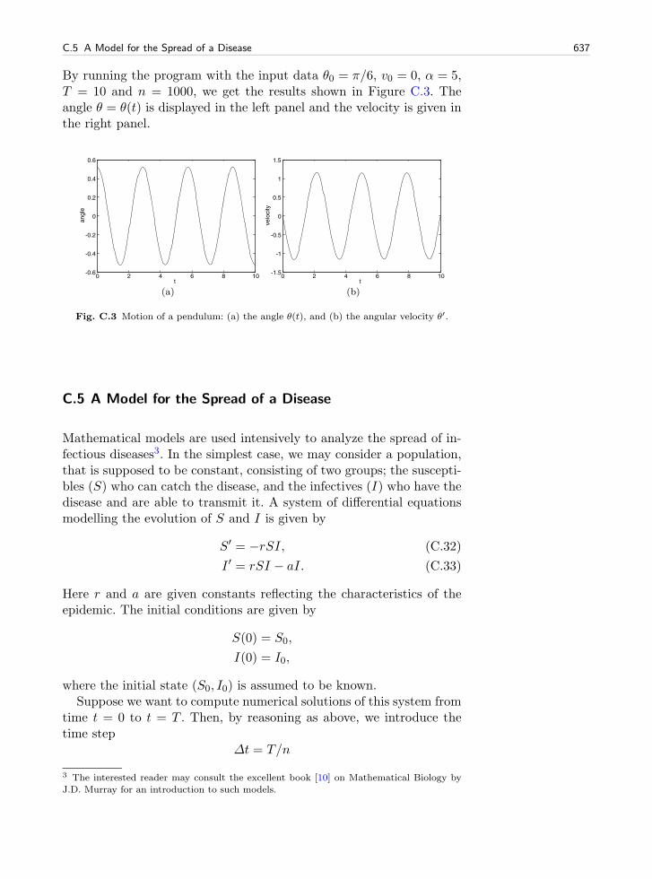
C.5 A Model for the Spread of a Disease 637
By running the program with the input data θ0 = π/6, v0 = 0, α = 5,T = 10 and n = 1000, we get the results shown in Figure C.3. Theangle θ = θ(t) is displayed in the left panel and the velocity is given inthe right panel.
Fig. C.3 Motion of a pendulum: (a) the angle θ(t), and (b) the angular velocity θ′.
C.5 A Model for the Spread of a Disease
Mathematical models are used intensively to analyze the spread of in-fectious diseases3. In the simplest case, we may consider a population,that is supposed to be constant, consisting of two groups; the suscepti-bles (S) who can catch the disease, and the infectives (I) who have thedisease and are able to transmit it. A system of differential equationsmodelling the evolution of S and I is given by
S′ = −rSI, (C.32)
I ′ = rSI − aI. (C.33)
Here r and a are given constants reflecting the characteristics of theepidemic. The initial conditions are given by
S(0) = S0,
I(0) = I0,
where the initial state (S0, I0) is assumed to be known.Suppose we want to compute numerical solutions of this system from
time t = 0 to t = T . Then, by reasoning as above, we introduce thetime step
Δt = T/n
3 The interested reader may consult the excellent book [10] on Mathematical Biology by
J.D. Murray for an introduction to such models.

638 C Introduction to Differential Equations
and the approximations (Sk, Ik) of the solution (S(tk), I(tk)). An ex-plicit Forward Euler method for the system takes the following form,
Sk+1 − Sk
Δt= −rSkIk,
Ik+1 − IkΔt
= rSkIk − aIk,
which can be rewritten on computational form
Sk+1 = Sk −ΔtrSkIk,
Ik+1 = Ik +Δt(rSkIk − aIk).
This scheme is implemented in the program exp_epidemic.py wherer, a, S0, I0, n and T are input data given on the command line. Thefunction epidemic computes the solution (S, I) to the differential equa-tion system. This pair of time-dependent functions is then plotted intwo separate plots.
def epidemic(T, n, S0, I0, r, a):dt = T/float(n)t = linspace(0, T, n+1)S = zeros(n+1)I = zeros(n+1)S[0] = S0I[0] = I0for k in range(n):
S[k+1] = S[k] - dt*r*S[k]*I[k]I[k+1] = I[k] + dt*(r*S[k]*I[k] - a*I[k])
return S, I, t
from scitools.std import *n = int(sys.argv[1])T = eval(sys.argv[2])S0 = eval(sys.argv[3])I0 = eval(sys.argv[4])r = eval(sys.argv[5])a = eval(sys.argv[6])
S, I, t = epidemic(T, n, S0, I0, r, a)plot(t, S, xlabel=’t’, ylabel=’Susceptibles’)plot(t, I, xlabel=’t’, ylabel=’Infectives’)
We want to apply the program to a specific case where an influenzaepidemic hit a British boarding school with a total of 763 boys4. Theepidemic lasted from 21st January to 4th February in 1978. We lett = 0 denote 21st of January and we define T = 14 days. We putS0 = 762 and I0 = 1 which means that one person was ill at t = 0.In the Figure C.4 we see the numerical results using r = 2.18 × 10⁻³,a = 0.44, n = 1000. Also, we have plotted actual the measurements,and we note that the simulations fit the real data quite well.
4 The data are from Murray [10], and Murray found the data in the British Medical Journal,
March 4, 1978.
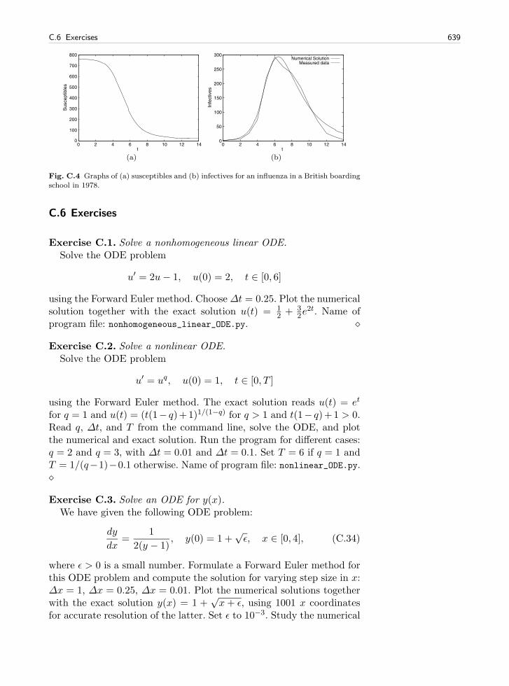
C.6 Exercises 639
Fig. C.4 Graphs of (a) susceptibles and (b) infectives for an influenza in a British boarding
school in 1978.
C.6 Exercises
Exercise C.1. Solve a nonhomogeneous linear ODE.Solve the ODE problem
u′ = 2u− 1, u(0) = 2, t ∈ [0, 6]
using the Forward Euler method. ChooseΔt = 0.25. Plot the numericalsolution together with the exact solution u(t) = 1
2 + 32e
2t. Name ofprogram file: nonhomogeneous_linear_ODE.py. �
Exercise C.2. Solve a nonlinear ODE.Solve the ODE problem
u′ = uq, u(0) = 1, t ∈ [0, T ]
using the Forward Euler method. The exact solution reads u(t) = et
for q = 1 and u(t) = (t(1− q)+1)1/(1−q) for q > 1 and t(1− q)+1 > 0.Read q, Δt, and T from the command line, solve the ODE, and plotthe numerical and exact solution. Run the program for different cases:q = 2 and q = 3, with Δt = 0.01 and Δt = 0.1. Set T = 6 if q = 1 andT = 1/(q−1)−0.1 otherwise. Name of program file: nonlinear_ODE.py.�
Exercise C.3. Solve an ODE for y(x).We have given the following ODE problem:
dy
dx=
1
2(y − 1), y(0) = 1 +
√ε, x ∈ [0, 4], (C.34)
where ε > 0 is a small number. Formulate a Forward Euler method forthis ODE problem and compute the solution for varying step size in x:Δx = 1, Δx = 0.25, Δx = 0.01. Plot the numerical solutions togetherwith the exact solution y(x) = 1 +
√x+ ε, using 1001 x coordinates
for accurate resolution of the latter. Set ε to 10−3. Study the numerical

640 C Introduction to Differential Equations
solution with Δx = 1, and use that insight to explain why this problemis hard to solve numerically. Name of program file: yx_ODE.py. �
Exercise C.4. Experience instability of an ODE.Consider the ODE problem
u′ = αu, u(0) = u0,
solved by the Forward Euler method. Show by repeatedly applying thescheme that
uk = (1 + αΔt)ku0.
We now turn to the case α < 0. Show that the numerical solution willoscillate if Δt > −1/α. Make a program for computing uk, set α = −1,and demonstrate oscillatory solutions for Δt = 1.1, 1.5, 1.9. Recall thatthe exact solution, u(t) = eαt, never oscillates.
What happens if Δt > −2/α? Try it out in the program and explainthen mathematically why not uk → 0 as k → ∞. Name of program file:unstable_ODE.py. �
Exercise C.5. Solve an ODE with time-varying growth.Consider the ODE for exponential growth,
u′ = αu, u(0) = 1, t ∈ [0, T ].
Now we introduce a time-dependent α such that the growth decreaseswith time: α(t) = a − bt. Solve the problem for a = 1, b = 0.1, andT = 10. Plot the solution and compare with the corresponding expo-nential growth using the mean value of α(t) as growth factor: e(a−bT/2)t.Name of program file: time_dep_growth.py. �

A Complete Differential Equation Project D
The examples in the ordinary chapters of this book are quite compactand composed to convey programming constructs in a gentle pedagog-ical way. In this appendix the idea is to solve a more comprehensivereal-world problem by programming. The problem solving process getsquite advanced because we bring together elements from physics, math-ematics, and programming, in a way that a scientific programmer mustmaster. Each individual element is quite straightforward in the sensethat you have probably met the element already, either in high schoolphysics or mathematics, or in this book. The challenge is to under-stand the problem, and analyze it by breaking it into a set of simplerelements. It is not necessary to understand this problem solving pro-cess in detail. As a computer programmer, all you need to understandis how you translate the given algorithm into a working program andhow to test the program. We anticipate that this task should be doablewithout a thorough understanding of the physics and mathematics ofthe problem.
You can read the present appendix after the material from Chap-ters 1–5 is are digested. More specifically, you can read Appendices D.1and D.2 after Chapter 4, while Appendix D.3 requires knowledge aboutcurve plotting from Chapter 5.
All Python files associated with this appendix are found insrc/box_spring.
D.1 About the Problem: Motion and Forces in Physics
D.1.1 The Physical Problem
We shall study a simple device which models oscillating systems. A boxwith mass m and height b is attached to a spring of length L as shownin Figure D.1. The end of the spring is attached to a plate which we
H.P. Langtangen, A Primer on Scientific Programming with Python,Texts in Computational Science and Engineering 6,
DOI 10.1007/978-3-642-30293-0, c© Springer-Verlag Berlin Heidelberg 2012
641

642 D A Complete Differential Equation Project
can move up and down with a displacement w(t), where t denotes time.There are two ways the box can be set in motion: we can either stretchor compress the string initially by moving the box up or down, or wecan move the plate. If w = 0 the box oscillates freely, otherwise wehave what is called driven oscillations.
Fig. D.1 An oscillating system with a box attached to a spring.
Why will such a system oscillate? When the box moves down-ward, the spring is stretched, which results in a force that tries tomove the box upward. The more we stretch the spring, the biggerthe force against the movement becomes. The box eventually stopsand starts moving upward with an upward acceleration. At somepoint the spring is not stretched anymore and there is no springforce on the box, but because of inertia, the box continues its mo-tion upward. This causes the spring to get compressed, causing a forcefrom the spring on the box that acts downward, against the upwardmovement. The downward force increases in intensity and managesto stop the upward motion. The process repeats itself and resultsin an oscillatory motion of the box. Since the spring tries to restorethe position of the box, we refer to the spring force as a restoringforce.
You have probably experienced that oscillations in such springs tendto die out with time. There is always a damping force that works againstthe motion. This damping force may be due to a not perfectly elasticstring, and the force can be quite small, but we can also explicitly attachthe spring to a damping mechanism to obtain a stronger, controllabledamping of the oscillations (as one wants in a car or a mountain bike).We will assume that there is some damping force present in our sys-

D.1 About the Problem: Motion and Forces in Physics 643
tem, and this can well be a damping mechanism although this is notexplicitly included in Figure D.1.
Oscillating systems of the type depicted in Figure D.1 have a hugenumber of applications throughout science and technology. One simpleexample is the spring system in a car or bicycle, which you have proba-bly experienced on a bumpy road (the bumps lead to a w(t) function).When your washing machine jumps up and down, it acts as a highlydamped oscillating system (and the w(t) function is related to unevendistribution of the mass of the clothes). The pendulum in a wall clock isanother oscillating system, not with a spring, but physically the systemcan (for small oscillations) be modeled as a box attached to a springbecause gravity makes a spring-like force on a pendulum (in this case,w(t) = 0). Other examples on oscillating systems where this type ofequation arise are briefly mentioned in Exercise E.44. The bottom lineis that understanding the dynamics of Figure D.1 is the starting pointfor understanding the behavior of a wide range of oscillating phenom-ena in nature and technical devices.
Goal of the Computations. Our aim is to compute the position of thebox as a function of time. If we know the position, we can compute thevelocity, the acceleration, the spring force, and the damping force. Themathematically difficult thing is to calculate the position – everythingelse is much easier1.
We assume that the box moves in the vertical direction only, so weintroduce Y (t) as the vertical position of the center point of the box.We shall derive a mathematical equation that has Y (t) as solution. Thisequation can be solved by an algorithm which can be implemented ina program. Our focus is on the implementation, since this is a bookabout programming, but for the reader interested in how computersplay together with physics and mathematics in science and technology,we also outline how the equation and algorithm arise.
The Key Quantities. Let S be the stretch of the spring, where S > 0means stretch and S < 0 implies compression. The length of the springwhen it is unstretched is L, so at a given point of time t the actuallength is L+ S(t). Given the position of the plate, w(t), the length ofthe spring, L+ S(t), and the height of the box, b, the position Y (t) isthen, according to Figure D.1,
Y (t) = w(t)−(L+ S(t)
)− b
2. (D.1)
1 More precisely, to compute the position we must solve a differential equation while the
other quantities can be computed by differentiation and simple arithmetics. Solving differ-ential equations is historically considered very difficult, but computers have simplified this
task dramatically. Appendices C and E are devoted to this topic.

644 D A Complete Differential Equation Project
You can think as follows: We first “go up” to the plate at y = w(t),then down L+ S(t) along the spring and then down b/2 to the centerof the box. While L, w, and b must be known as input data, S(t) isunknown and will be output data from the program.
D.1.2 The Computational Algorithm
Let us now go straight to the programming target and present the recipefor computing Y (t). The algorithm below actually computes S(t), butat any point of time we can easily find Y (t) from (D.1) if we know S(t).The S(t) function is computed at discrete points of time, t = ti = iΔt,for i = 0, 1, . . . , N . We introduce the notation Si for S(ti). The Si
values can be computed by the following algorithm.
1. Set initial stretch S0 from input data2. Compute S1 by
Si+1 =1
2m
(2mSi−Δt2 kSi+m(wi+1−2wi+wi−1)+Δt2mg
), (D.2)
with i = 0.3. For i = 1, 2, . . . , N − 1, compute Si+1 by
Si+1 = (m+ γ)−1(2mSi −mSi−1 + γΔtSi−1 −Δt2 kSi
+m(wi+1 − 2wi + wi−1) +Δt2mg). (D.3)
The parameter γ equals 12βΔt. The input data to the algorithm are the
mass of the boxm, a coefficient k characterizing the spring, a coefficientβ characterizing the amount of damping in the system, the accelerationof gravity g, the movement of the plate w(t), the initial stretch of thespring S0, the number of time steps N , and the time Δt between eachcomputation of S values. The smaller we choose Δt, the more accuratethe computations become.
Now you have two options, either read the derivation of this algo-rithm in Appendix D.1.3–D.1.4 or jump right to implementation inAppendix D.2.
D.1.3 Derivation of the Mathematical Model
To derive the algorithm we need to make a mathematical model ofthe oscillating system. This model is based on physical laws. The mostimportant physical law for a moving body is Newton’s second law ofmotion:
F = ma, (D.4)
where F is the sum of all forces on the body, m is the mass of the body,and a is the acceleration of the body. The body here is our box.

D.1 About the Problem: Motion and Forces in Physics 645
Let us first find all the forces on the box. Gravity acts downwardwith magnitude mg. We introduce Fg = −mg as the gravity force,with a minus sign because a negative force acts downward, in negativey direction.
The spring force on the box acts upward if the spring is stretched,i.e., if S > 0 we have a positive spring force Fs. The size of the force isproportional to the amount of stretching, so we write2 Fs = kS, wherek is commonly known as the spring constant. We also assume that wehave a damping force that is always directed toward the motion andproportional with the “velocity of the stretch”, −dS/dt. Naming theproportionality constant β, we can write the damping force as Fd =βdS/dt. Note that when dS/dt > 0, S increases in time and the boxmoves downward, the Fd force then acts upward, against the motion,and must be positive. This is the way we can check that the dampingforce expression has the right sign.
The sum of all forces is now
F = Fg + Fs + Fd,
= −mg + kS + βdS
dt. (D.5)
We now know the left-hand side of (D.4), but S is unknown to us.The acceleration a on the right-hand side of (D.4) is also unknown.However, acceleration is related to movement and the S quantity, andthrough this relation we can eliminate a as a second unknown. Fromphysics, it is known that the acceleration of a body is the second deriva-tive in time of the position of the body, so in our case,
a =d2Y
dt2,
=d2w
dt2− d2S
dt2, (D.6)
(remember that L and b are constant).Equation (D.4) now reads
−mg + kS + βdS
dt= m
(d2w
dt2− d2S
dt2
). (D.7)
It is common to collect the unknown terms on the left-hand side and theknown quantities on the right-hand side, and let higher-order deriva-tives appear before lower-order derivatives. With such a reordering ofterms we get
2 Spring forces are often written in the canonical form “F = −kx”, where x is the stretch.The reason that we have no minus sign is that our stretch S is positive in the downward
(negative) direction.

646 D A Complete Differential Equation Project
md2S
dt2+ β
dS
dt+ kS = m
d2w
dt2+mg. (D.8)
This is the equation governing our physical system. If we solve theequation for S(t), we have the position of the box according to (D.1),the velocity v as
v(t) =dY
dt=
dw
dt− dS
dt, (D.9)
the acceleration as (D.6), and the various forces can be easily obtainedfrom the formulas in (D.5).
A key question is if we can solve (D.8). If w = 0, there is in fact awell-known solution which can be written
S(t) =m
kg +
⎧⎨⎩
e−ζt(c1et√β2−1 + c2e
−t√ζ2−1), ζ > 1,
e−ζt(c1 + c2t), ζ = 1,
e−ζt[c1 cos(√
1− ζ2t) + c2 sin(√
1− ζ2t)], ζ < 1.(D.10)
Here, ζ is a short form for β/2, and c1 and c2 are arbitrary constants.That is, the solution (D.10) is not unique.
To make the solution unique, we must determine c1 and c2. This isdone by specifying the state of the system at some point of time, sayt = 0. In the present type of mathematical problem we must specify Sand dS/dt. We allow the spring to be stretched an amount S0 at t = 0.Moreover, we assume that there is no ongoing increase or decrease inthe stretch at t = 0, which means that dS/dt = 0. In view of (D.9), thiscondition implies that the velocity of the box is that of the plate, andif the latter is at rest, the box is also at rest initially. The conditionsat t = 0 are called initial conditions :
S(0) = S0,dS
dt(0) = 0. (D.11)
These two conditions provide two equations for the two unknown con-stants c1 and c2. Without the initial conditions two things happen: (i)there are infinitely many solutions to the problem, and (ii) the compu-tational algorithm in a program cannot start.
Also when w �= 0 one can find solutions S(t) of (D.8) in terms ofmathematical expressions, but only for some very specific choices ofw(t) functions. With a program we can compute the solution S(t) forany “reasonable” w(t) by a quite simple method. The method givesonly an approximate solution, but the approximation can usually bemade as good as desired. This powerful solution method is describedbelow.
D.1.4 Derivation of the Algorithm
To solve (D.8) on a computer, we do two things:

D.1 About the Problem: Motion and Forces in Physics 647
1. We calculate the solution at some discrete time points t = ti = iΔt,i = 0, 1, 2, . . . , N .
2. We replace the derivatives by finite differences, which are approxi-mate expressions for the derivatives.
The first and second derivatives can be approximated by3
dS
dt(ti) ≈
S(ti+1)− S(ti−1)
2Δt, (D.12)
d2S
dt2(ti) ≈
S(ti+1)− 2S(ti) + S(ti−1)
Δt2. (D.13)
It is common to save some writing by introducing Si as a short formfor S(ti). The formulas then read
dS
dt(ti) ≈
Si+1 − Si−1
2Δt, (D.14)
d2S
dt2(ti) ≈
Si+1 − 2Si + Si−1
Δt2. (D.15)
Let (D.8) be valid at a point of time ti:
md2S
dt2(ti) + β
dS
dt(ti) + kS(ti) = m
d2w
dt2(ti) +mg. (D.16)
We now insert (D.14) and (D.15) in (D.16) (observe that we can ap-proximate d2w/dt2 in the same way as we approximate d2S/dt2):
mSi+1 − 2Si + Si−1
Δt2+β
Si+1 − Si−1
2Δt+kSi = m
wi+1 − 2wi + wi−1
Δt2+mg.
(D.17)The computational algorithm starts with knowing S0, then S1 is com-puted, then S2, and so on. Therefore, in (D.17) we can assume that Si
and Si−1 are already computed, and that Si+1 is the new unknown tocalculate. Let us as usual put the unknown terms on the left-hand side(and multiply by Δt2):
mSi+1 + γSi+1 = 2mSi −mSi−1 + γSi−1 −Δt2 kSi
+m(wi+1 − 2wi + wi−1) +Δt2mg, (D.18)
where we have introduced the short form γ = 12βΔt to save space.
Equation (D.18) can easily be solved for Si+1:
Si+1 = (m+ γ)−1(2mSi −mSi−1 + γΔtSi−1 −Δt2 kSi
+m(wi+1 − 2wi + wi−1) +Δt2mg). (D.19)
One fundamental problem arises when we try to start the computa-tions. We know S0 and want to apply (D.19) for i = 0 to calculate S1.
3 See Appendices B and C for derivations of such formulas.

648 D A Complete Differential Equation Project
However, (D.19) involves Si−1, that is, S−1, which is an unknown valueat a point of time before we compute the motion. The initial condi-tions come to rescue here. Since dS/dt = 0 at t = 0 (or i = 0), we canapproximate this condition as
S1 − S−1
2Δt= 0 ⇒ S−1 = S1. (D.20)
Inserting this relation in (D.19) when i = 0 gives a special formula forS1 (or Si+1 with i = 0, if we want):
Si+1 =1
2m
(2mSi−Δt2 kSi+m(wi+1−2wi+wi−1)+Δt2mg
). (D.21)
Remember that i = 0 in this formula. The overall algorithm is summa-rized below:
1. Initialize S0 from initial condition2. Use (D.21) to compute Si+1 for i = 03. For i = 0, 1, 2, . . . , N − 1, use (D.19) to compute Si+1
D.2 Program Development and Testing
D.2.1 Implementation
The aim now is to implement the algorithm on page 644 in a Pythonprogram. There are naturally two parts of the program, one where weread input data such as L, m, and w(t), and one part where we runthe computational algorithm. Let us write a function for each part.
The set of input data to the program consists of the mathematicalsymbols
• m (the mass of the box)• b (the height of the box)• L (the length of the unstretched spring)• β (coefficient for the damping force)• k (coefficient for the spring force)• Δt (the time step between each Si calculation)• N (the number of computed time steps)• S0 (the initial stretch of the spring)• w(t) (the vertical displacement of the plate)• g (acceleration of gravity)
We make a function init_prms for initializing these input parametersfrom option-value pairs on the command line. That is, the user pro-vides pairs like -m 2 and -dt 0.1 (for Δt). The argparse module fromChapter 4.2.4 can be used for this purpose. We supply default valuesfor all parameters as arguments to the init_prms function. The func-

D.2 Program Development and Testing 649
tion returns all these parameters with the changes that the user hasspecified on the command line. The w parameter is given as a stringexpression (called w_formula below), and the StringFunction tool fromChapter 4.1.4 can be used to turn the formula into a working Pythonfunction. An algorithmic sketch of the tasks in the init_prms functioncan be expressed by some pseudo Python code:
def init_prms(m, b, L, k, beta, S0, dt, g, w_formula, N):import argparseparser = argparse.ArgumentParser()parser.add_argument(’--m’, ’--mass’,
type=float, default=m)parser.add_argument(’--b’, ’--boxheight’,
type=float, default=b)...args = parser.parse_args()
from scitools.StringFunction import StringFunctionw = StringFunction(args.w, independent_variables=’t’)return args.m, args.b, args.L, args.k, args.beta, \
args.S0, args.dt, args.g, w, args.N
With such a sketch as a start, we can complete the indicated codeand arrive at a working function for specifying input parameters to themathematical model:
def init_prms(m, b, L, k, beta, S0, dt, g, w_formula, N):import argparseparser = argparse.ArgumentParser()parser.add_argument(’--m’, ’--mass’,
type=float, default=m)parser.add_argument(’--b’, ’--boxheight’,
type=float, default=b)parser.add_argument(’--L’, ’--spring-length’,
type=float, default=L)parser.add_argument(’--k’, ’--spring-stiffness’,
type=float, default=k)parser.add_argument(’--beta=’, ’--spring-damping’,
type=float, default=beta)parser.add_argument(’--S0’, ’--initial-position’,
type=float, default=S0)parser.add_argument(’--dt’,’--timestep’,
type=float, default=dt)parser.add_argument(’--g’, ’--gravity’,
type=float, default=g)parser.add_argument(’--w’, type=float, default=w)parser.add_argument(’--N’, type=int, default=N)args = parser.parse_args()
from scitools.StringFunction import StringFunctionw = StringFunction(args.w, independent_variables=’t’)return args.m, args.b, args.L, args.k, args.beta, \
args.S0, args.dt, args.g, w, args.N
You may wonder why we specify g (gravity) since this is a known con-stant, but it is useful to turn off the gravity force to test the program.Just imagine the oscillations take place in the horizontal direction –the mathematical model is the same, but Fg = 0, which we can obtainin our program by setting the input parameter g to zero.

650 D A Complete Differential Equation Project
The computational algorithm is quite easy to implement, as thereis a quite direct translation of the mathematical algorithm in Ap-pendix D.1.2 to valid Python code. The Si values can be stored ina list or array with indices going from 0 to N . To allow readers tofollow the code here without yet having digested Chapter 5, we use aplain list. The function for computing Si reads
def solve(m, k, beta, S0, dt, g, w, N):S = [0.0]*(N+1) # output listgamma = beta*dt/2.0 # short formt = 0S[0] = S0# Special formula for first time stepi = 0S[i+1] = (1/(2.0*m))*(2*m*S[i] - dt**2*k*S[i] +
m*(w(t+dt) - 2*w(t) + w(t-dt)) + dt**2*m*g)t = dt
for i in range(1,N):S[i+1] = (1/(m + gamma))*(2*m*S[i] - m*S[i-1] +
gamma*dt*S[i-1] - dt**2*k*S[i] +m*(w(t+dt) - 2*w(t) + w(t-dt))+ dt**2*m*g)
t += dtreturn S
The primary challenge in coding the algorithm is to set the index i
and the time t right. Recall that in the updating formula for S[i+1]
at time t+dt, the time on the right-hand side shall be the time attime step i, so the t+=dt update must come after S[i+1] is computed.The same is important in the special formula for the first time step aswell.
A main program will typically first set some default values of the 10input parameters, then call init_prms to let the user adjust the defaultvalues, and then call solve to compute the Si values:
# Default valuesfrom math import pim = 1; b = 2; L = 10; k = 1; beta = 0; S0 = 1;dt = 2*pi/40; g = 9.81; w_formula = ’0’; N = 80;
m, b, L, k, beta, S0, dt, g, w, N = \init_prms(m, b, L, k, beta, S0, dt, g, w_formula, N)
S = solve(m, k, beta, S0, dt, g, w, N)
So, what shall we do with the solution S? We can write out thevalues of this list, but the numbers do not give an immediate feel-ing for how the box moves. It will be better to graphically illus-trate the S(t) function, or even better, the Y (t) function. This isstraightforward with the techniques from Chapter 5 and is treatedin Appendix D.3. In Chapter 9.4, we develop a drawing tool fordrawing figures like Figure D.1. By drawing the box, string, andplate at every time level we compute Si, we can use this tool tomake a moving figure that illustrates the dynamics of the oscilla-

D.2 Program Development and Testing 651
tions. Already now you can play around with a program doing that(box_spring_figure_anim.py).
D.2.2 Callback Functionality
It would be nice to make some graphics of the system while the com-putations take place, not only after the S list is ready. The user mustthen put some relevant statements in between the statements in thealgorithm. However, such modifications will depend on what type ofanalysis the user wants to do. It is a bad idea to mix user-specificstatements with general statements in a general algorithm. We there-fore let the user provide a function that the algorithm can call aftereach Si value is computed. This is commonly called a callback func-tion (because a general function calls back to the user’s program todo a user-specific task). To this callback function we send three keyquantities: the S list, the point of time (t), and the time step num-ber (i + 1), so that the user’s code gets access to these importantdata.
If we just want to print the solution to the screen, the callback func-tion can be as simple as
def print_S(S, t, step):print’t=%.2f S[%d]=%+g’ % (t, step, S[step])
In the solve function we take the callback function as a keyword argu-ment user_action. The default value can be an empty function, whichwe can define separately:
def empty_func(S, time, time_step_no):return None
def solve(m, k, beta, S0, dt, g, w, N,user_action=empty_func):
...
However, it is quicker to just use a lambda function (see Chap-ter 3.1.11):
def solve(m, k, beta, S0, dt, g, w, N,user_action=lambda S, time, time_step_no: None):
The new solve function has a call to user_action each time a new Svalue has been computed:
def solve(m, k, beta, S0, dt, g, w, N,user_action=lambda S, time, time_step_no: None):
"""Calculate N steps forward. Return list S."""S = [0.0]*(N+1) # output listgamma = beta*dt/2.0 # short formt = 0S[0] = S0

652 D A Complete Differential Equation Project
user_action(S, t, 0)# Special formula for first time stepi = 0S[i+1] = (1/(2.0*m))*(2*m*S[i] - dt**2*k*S[i] +
m*(w(t+dt) - 2*w(t) + w(t-dt)) + dt**2*m*g)t = dtuser_action(S, t, i+1)
# Time loopfor i in range(1,N):
S[i+1] = (1/(m + gamma))*(2*m*S[i] - m*S[i-1] +gamma*dt*S[i-1] - dt**2*k*S[i] +m*(w(t+dt) - 2*w(t) + w(t-dt))+ dt**2*m*g)
t += dtuser_action(S, t, i+1)
return S
The two last arguments to user_action must be carefully set: theseshould be time value and index for the most recently computed S value.
D.2.3 Making a Module
The init_prms and solve functions can now be combined with manydifferent types of main programs and user_action functions. It is there-fore preferable to have the general init_prms and solve functions in amodule box_spring and import these functions in more user-specificprograms. Making a module out of init_prms and solve is, accordingto Chapter 4.5, quite trivial as we just need to put the functions in afile box_spring.py.
It is always a good habit to include a test block in module files.To make the test block small, we place the statements in a separatefunction _test and just call _test in the test block. The initial under-score in the name _test prevents this function from being importedby a from box_spring import * statement. Our test here simply printssolution at each time level. The following code snippet is then addedto the module file to include a test block:
def _test():def print_S(S, t, step):
print ’t=%.2f S[%d]=%+g’ % (t, step, S[step])
# Default valuesfrom math import pim = 1; b = 2; L = 10; k = 1; beta = 0; S0 = 1;dt = 2*pi/40; g = 9.81; w_formula = ’0’; N = 80;
m, b, L, k, beta, S0, dt, g, w, N = \init_prms(m, b, L, k, beta, S0, dt, g, w_formula, N)
S = solve(m, k, beta, S0, dt, g, w, N,user_action=print_S)
if __name__ == ’__main__’:_test()

D.2 Program Development and Testing 653
D.2.4 Verification
To check that the program works correctly, we need a series of problemswhere the solution is known. These test cases must be specified bysomeone with a good physical and mathematical understanding of theproblem being solved. We already have a solution formula (D.10) thatwe can compare the computations with, and more tests can be madein the case w �= 0 as well.
However, before we even think of checking the program against theformula (D.10), we should perform some much simpler tests. The sim-plest test is to see what happens if we do nothing with the system.This solution is of course not very exciting – the box is at rest, butit is in fact exciting to see if our program reproduces the boring so-lution. Many bugs in the program can be found this way! So, let usrun the program box_spring.py with -S0 0 as the only command-lineargument. The output reads
t=0.00 S[0]=+0t=0.16 S[1]=+0.121026t=0.31 S[2]=+0.481118t=0.47 S[3]=+1.07139t=0.63 S[4]=+1.87728t=0.79 S[5]=+2.8789t=0.94 S[6]=+4.05154t=1.10 S[7]=+5.36626...
Something happens! All S[1], S[2], and so forth should be zero. Whatis the error?
There are two directions to follow now: we can either visualize thesolution to understand more of what the computed S(t) function lookslike (perhaps this explains what is wrong), or we can dive into thealgorithm and compute S[1] by hand to understand why it does notbecome zero. Let us follow both paths.
First we print out all terms on the right-hand side of the statementthat computes S[1]. All terms except the last one (Δt2mg) are zero.The gravity term causes the spring to be stretched downward, whichcauses oscillations. We can see this from the governing equation (D.8)too: If there is no motion, S(t) = 0, the derivatives are zero (and w = 0is default in the program), and then we are left with
kS = mg ⇒ S =m
kg. (D.22)
This result means that if the box is at rest, the spring is stretched(which is reasonable!). Either we have to start with S(0) = m
k g in theequilibrium position, or we have to turn off the gravity force by setting-g 0 on the command line. Setting either -S0 0 -g 0 or -S0 9.81 showsthat the whole S list contains either zeros or 9.81 values (recall thatm = k = 1 so S0 = g). This constant solution is correct, and the codinglooks promising.

654 D A Complete Differential Equation Project
We can also plot the solution using the program box_spring_plot:
Terminal
box_spring_plot.py --S0 0 --N 200
Figure D.2 shows the function Y (t) for this case where the initial stretchis zero, but gravity is causing a motion. With some mathematical anal-ysis of this problem we can establish that the solution is correct. Wehave that m = k = 1 and w = β = 0, which implies that the governingequation is
d2S
dt2+ S = g, S(0) = 0, dS/dt(0) = 0.
Without the g term this equation is simple enough to be solved bybasic techniques you can find in most introductory books on differentialequations. Let us therefore get rid of the g term by a little trick: weintroduce a new variable T = S − g, and by inserting S = T + g in theequation, the g is gone:
d2T
dt2+ T = 0, T (0) = −g,
dT
dt(0) = 0. (D.23)
This equation is of a very well-known type and the solution reads T (t) =−g cos t, which means that S(t) = g(1− cos t) and
Y (t) = −L− g(1− cos t)− b
2.
With L = 10, g ≈ 10, and b = 2 we get oscillations around y ≈ 21 witha period of 2π and a start value Y (0) = −L− b/2 = 11. A rough visualinspection of the plot shows that this looks right. A more thoroughanalysis would be to make a test of the numerical values in a newcallback function (the program is found in box_spring_test1.py):
from box_spring import init_prms, solvefrom math import cos
def exact_S_solution(t):return g*(1 - cos(t))
def check_S(S, t, step):error = exact_S_solution(t) - S[step]print ’t=%.2f S[%d]=%+g error=%g’ % (t, step, S[step], error)
# Fixed values for a testfrom math import pim = 1; b = 2; L = 10; k = 1; beta = 0; S0 = 0dt = 2*pi/40; g = 9.81; N = 200
def w(t):return 0
S = solve(m, k, beta, S0, dt, g, w, N, user_action=check_S)

D.3 Visualization 655
The output from this program shows increasing errors with time,up as large values as 0.3. The difficulty is to judge whether this is theerror one must expect because the program computes an approximatesolution, or if this error points to a bug in the program – or a wrongmathematical formula.
From these sessions on program testing you will probably realize thatverification of mathematical software is challenging. In particular, thedesign of the test problems and the interpretation of the numerical out-put require quite some experience with the interplay between physics(or another application discipline), mathematics, and programming.
Fig. D.2 Positions Y (t) of an oscillating box with m = k = 1, w = β = 0, g = 9.81,L = 10, and b = 2.
D.3 Visualization
The purpose of this section is to add graphics to the oscillating systemapplication developed in Appendix D.2. Recall that the function solve
solves the problem and returns a list S with indices from 0 to N. Ouraim is to plot this list and various physical quantities computed from it.
D.3.1 Simultaneous Computation and Plotting
The solve function makes a call back to the user’s code through acallback function (the user_action argument to solve) at each timelevel. The callback function has three arguments: S, the time, and thecurrent time step number. Now we want the callback function to plotthe position Y (t) of the box during the computations. In principle thisis easy, but S is longer than we want to plot, because S is allocated

656 D A Complete Differential Equation Project
for the whole time simulation while the user_action function is calledat time levels where only the indices in S up to the current time levelhave been computed (the rest of the elements in S are zero). We musttherefore use a sublist of S, from time zero and up to the current time.The callback function we send to solve as the user_action argumentcan then be written like this:
def plot_S(S, t, step):if step == 0: # nothing to plot yet
return None
tcoor = linspace(0, t, step+1)S = array(S[:len(tcoor)])Y = w(tcoor) - L - S - b/2.plot(tcoor, Y)
Note that L, dt, b, and w must be global variables in the user’s mainprogram.
The major problem with the plot_S function shown is that thew(tcoor) evaluation does not work. The reason is that w is aStringFunction object, and according to Chapter 5.5.1, StringFunctionobjects do not work with array arguments unless we call their vectorizefunction once. We therefore need to do a
w.vectorize(globals())
before calling solve (which calls plot_S repeatedly). Here is the mainprogram with this important statement:
from box_spring import init_prms, solvefrom scitools.std import *
# Default valuesm = 1; b = 2; L = 10; k = 1; beta = 0; S0 = 1;dt = 2*pi/40; g = 9.81; w_formula = ’0’; N = 200;
m, b, L, k, beta, S0, dt, g, w, N = \init_prms(m, b, L, k, beta, S0, dt, g, w_formula, N)
w.vectorize(globals())
S = solve(m, k, beta, S0, dt, g, w, N, user_action=plot_S)
Now the plot_S function works fine. You can try the program out byrunning
Terminal
box_spring_plot_v1.py
Fixing Axes. Both the t and the y axes adapt to the solution array inevery plot. The adaptation of the y is okay since it is difficult to predictthe future minimum and maximum values of the solution, and hence itis most natural to just adapt the y axis to the computed Y points sofar in the simulation. However, the t axis should be fixed throughout
D.3 Visualization 657
the simulation, and this is easy since we know the start and end times.The relevant plot call now becomes4
plot(tcoor, Y,axis=[0, N*dt, min(Y), max(Y)],xlabel=’time’, ylabel=’Y’)
At the end of the simulation it can be nice to make a hardcopy of thelast plot command performed in the plot_S function. We then justcall
savefig(’tmp_Y.eps’)
after the solve function is finished.In the beginning of the simulation it is convenient to skip plotting
for a number of steps until there are some interesting points to visualizeand to use for computing the axis extent. We also suggest to apply therecipe at the end of Chapter 5.5.1 to vectorize w. More precisely, we usew.vectorize in general, but turn to numpy’s vectorize feature only if thestring formula contains an inline if-else test (to avoid requiring usersto use where to vectorize the string expressions). One reason for payingattention to if-else tests in the w formula is that sudden movementsof the plate are of interest, and this gives rise to step functions andstrings like ’1 if t>0 else 0’. A main program with all these featuresis listed next.
from box_spring import init_prms, solvefrom scitools.std import *
def plot_S(S, t, step):first_plot_step = 10 # skip the first stepsif step < first_plot_step:
return
tcoor = linspace(0, t, step+1) # t = dt*stepS = array(S[:len(tcoor)])Y = w(tcoor) - L - S - b/2.0 # (w, L, b are global vars.)
plot(tcoor, Y,axis=[0, N*dt, min(Y), max(Y)],xlabel=’time’, ylabel=’Y’)
# Default valuesm = 1; b = 2; L = 10; k = 1; beta = 0; S0 = 1dt = 2*pi/40; g = 9.81; w_formula = ’0’; N = 200
m, b, L, k, beta, S0, dt, g, w, N = \init_prms(m, b, L, k, beta, S0, dt, g, w_formula, N)
# Vectorize the StringFunction ww_formula = str(w) # keep this to see if w=0 laterif ’ else ’ in w_formula:
w = vectorize(w) # general vectorizationelse:
w.vectorize(globals()) # more efficient (when no if)
4 Note that the final time is T = NΔt.

658 D A Complete Differential Equation Project
S = solve(m, k, beta, S0, dt, g, w, N, user_action=plot_S)
# First make a hardcopy of the last plot of Yhardcopy(’tmp_Y.eps’)
D.3.2 Some Applications
What if we suddenly, right after t = 0, move the plate upward fromy = 0 to y = 1? This will set the system in motion, and the task is tofind out what the motion looks like.
There is no initial stretch in the spring, so the initial condition be-comes S0 = 0. We turn off gravity for simplicity and try a w = 1function since the plate has the position y = w = 1 for t > 0:
Terminal
box_spring_plot.py --w’1’ --S 0 --g 0
Nothing happens. The reason is that we specify w(t) = 1, but in theequation only d2w/dt2 has an effect and this quantity is zero. What weneed to specify is a step function: w = 0 for t ≤ 0 and w = 1 for t > 0.In Python such a function can be specified as a string expression ’1 if
t>0 else 0’. With a step function we obtain the right initial jump ofthe plate:
Terminal
box_spring_plot.py --w’1 if t > 0 else 0’ \--S0 0 --g 0 --N 1000 --beta 0.1
Figure D.3 displays the solution. We see that the damping parameterhas the effect of reducing the amplitude of Y (t), and the reductionlooks exponential, which is in accordance with the exact solution (D.10)(although this formula is not valid in the present case because w �= 0– but one gets the same exponential reduction even in this case). Thebox is initially located in Y = 0 − (10 + 0) − 2/2 = −11. During thefirst time step we get a stretch S = 0.5 and the plate jumps up toy = 1 so the box jumps to Y = 1 − (10 + 0.5) − 2/2 = −10.5. InFigure D.3b we that the box starts correctly out and jumps upwards,as expected.
More exciting motions of the box can be obtained by moving theplate back and forth in time, see for instance Figure D.4 on page 661.
D.3.3 Remark on Choosing Δt
If you run the box_spring_plot.py program with a large -dt argument(for Δt), strange things may happen. Try -dt 2 -N 20 as command-line arguments and observe that Y jumps up and down in a saw tooth

D.3 Visualization 659
Fig. D.3 Plot of the position of an oscillating box where the end point of the spring (w(t))is given a sudden movement at t = 0. Other parameters are m = k = 1, β = 0.1, g = 0,
S0 = 0. (a) 1000 time steps; (b) 100 steps for magnifying the first oscillation cycles.
fashion so we clearly have too large time steps. Then try -dt 2.1 -N 20
and observe that Y takes on very large values (105). This highly non-physical result points to an error in the program. However, the problemis not in the program, but in the numerical method used to solve (D.8).This method becomes unstable and hence useless if Δt is larger thana critical value. We shall not dig further into such problems, but justnotice that mathematical models on a computer must be used with care,and that a serious user of simulation programs must understand howthe mathematical methods work in detail and what their limitationsare.
D.3.4 Comparing Several Quantities in Subplots
So far we have plotted Y , but there are other interesting quantities tolook at, e.g., S, w, the spring force, and the damping force. The springforce and S are proportional, so only one of these is necessary to plot.Also, the damping force is relevant only if β �= 0, and w is only relevantif the string formula is different from the default value ’0’.
All the mentioned additional plots can be placed in the same fig-ure for comparison. To this end, we apply the subfigure command inEasyviz and create a row of individual plots. How many plots we havedepends on the values of str(w) and beta. The relevant code snippetfor creating the additional plots is given below and appears after thepart of the main program shown above.
# Make plots of several additional interesting quantitiestcoor = linspace(0, tstop, N+1)S = array(S)
plots = 2 # number of rows of plotsif beta != 0:
plots += 1if w_formula != ’0’:
plots += 1

660 D A Complete Differential Equation Project
# Position Y(t)plot_row = 1subplot(plots, 1, plot_row)Y = w(tcoor) - L - S - b/2.0plot(tcoor, Y, xlabel=’time’, ylabel=’Y’)
# Spring force (and S)plot_row += 1subplot(plots, 1, plot_row)Fs = k*Splot(tcoor, Fs, xlabel=’time’, ylabel=’spring force’)
# Friction forceif beta != 0:
plot_row += 1subplot(plots, 1, plot_row)Fd = beta*diff(S) # diff is in numpy# len(diff(S)) = len(S)-1 so we use tcoor[:-1]:plot(tcoor[:-1], Fd, xlabel=’time’, ylabel=’damping force’)
# Excitationif w_formula != ’0’:
plot_row += 1subplot(plots, 1, plot_row)w_array = w(tcoor)plot(tcoor, w_array, xlabel=’time’, ylabel=’w(t)’)
savefig(’tmp.eps’) # save this multi-axis plot in a file
Figure D.4 displays what the resulting plot looks like for a test casewith an oscillating plate (w). The command for this run is
Terminal
box_spring_plot.py --S0 0 --w’2*(cos(8*t)-1)’ \--N 600 --dt 0.05236
The rapid oscillations of the plate require us to use a smaller Δt andmore steps (larger N).
D.3.5 Comparing Approximate and Exact Solutions
To illustrate multiple curves in the same plot and animations we turnto a slightly different program. The task now is to visually investigatehow the accuracy of the computations depends on the Δt parameter.The smaller Δt is, the more accurate the solution S is. To look intothis topic, we need a test problem with known solution. Setting m =k = 1 and w = 0 = β = 0 implies the exact solution S(t) = g(1 −cos t) (see Appendix D.2.4). The box_spring_test1.py program fromAppendix D.2.4 can easily be extended to plot the calculated solutiontogether with the exact solution. We drop the user_action callbackfunction and just make the plot after having the complete solution S
returned from the solve function:

D.3 Visualization 661
Fig. D.4 Plot of the plate position w(t), the spring force (proportional to S(t)), and theposition Y (t) for a test problem where w(t) = 2(cos(8t)−1), β = g = 0, m = k = 1, S0 = 0,
Δt = 0.5236, and N = 600.
tcoor = linspace(0, N*dt, len(S))exact = exact_S_solution(tcoor)plot(tcoor, S, ’r’, tcoor, exact, ’b’,
xlabel=’time’, ylabel=’S’,legend=(’computed S(t)’, ’exact S(t)’),savefig=’tmp_S.eps’)
The two curves tend to lie upon each other, so to get some more insightinto the details of the error, we plot the error itself, in a separate plotwindow:
figure() # new plot windowS = array(S) # turn list into NumPy array for computationserror = exact - Splot(tcoor, error, xlabel=’time’, ylabel=’error’,
savefig=’tmp_error.eps’)
The error increases in time as the plot in Figure D.5a clearly shows.
D.3.6 Evolution of the Error as Δt Decreases
Finally, we want to investigate how the error curve evolves as the timestepΔt decreases. In a loop we halveΔt in each pass, solve the problem,compute the error, and plot the error curve. From the finite differenceformulas involved in the computational algorithm, we can expect thatthe error is of order Δt2. That is, if Δt is halved, the error should bereduced by 1/4.
The resulting plot of error curves is not very informative because theerror reduces too quickly (by several orders of magnitude). A better plot

662 D A Complete Differential Equation Project
is obtained by taking the logarithm of the error. Since an error curvemay contain positive and negative elements, we take the absolute valueof the error before taking the logarithm. We also note that S0 is alwayscorrect, so it is necessary to leave out the initial value of the error arrayto avoid the logarithm of zero.
The ideas of the previous two paragraphs can be summarized in aPython code snippet:
figure() # new plot windowdt = 2*pi/10tstop = 8*pi # 4 periodsN = int(tstop/dt)for i in range(6):
dt /= 2.0N *= 2S = solve(m, k, beta, S0, dt, g, w, N)S = array(S)tcoor = linspace(0, tstop, len(S))exact = exact_S_solution(tcoor)abserror = abs(exact - S)# Drop abserror[0] since it is always zero and causes# problems for the log function:logerror = log10(abserror[1:])
plot(tcoor[1:], logerror, ’r’, xlabel=’time’,ylabel=’log10(abs(error))’)
hold(’on’)savefig(’tmp_errors.eps’)
The resulting plot is shown in Figure D.5b.
Fig. D.5 Error plots for a test problem involving an oscillating system: (a) the error as a
function of time; (b) the logarithm of the absolute value of the error as a function of time,where Δt is reduced by one half from one curve to the next one below.
Visually, it seems to be a constant distance between the curves inFigure D.5b. Let d denote this difference and let Ei be the absoluteerror curve associated with Δt in the i-th pass in the loop. What weplot is log10Ei. The difference between two curves is then Di+1 =log10Ei − log10Ei+1 = log10(Ei/Ei+1). If this difference is roughly 0.5as we see from Figure D.5b, we have

D.3 Visualization 663
log10Ei
Ei+1= d = 0.5 ⇒ Ei+1 =
1
3.16Ei.
That is, the error is reduced, but not by the theoretically expectedfactor 4. Let us investigate this topic in more detail by plotting Di+1.
We make a loop as in the last code snippet, but store the logerror ar-ray from the previous pass in the loop (Ei) in a variable logerror_prev
such that we can compute the difference Di+1 as
logerror_diff = logerror_prev - logerror
There are two problems to be aware of now in this array subtraction:(i) the logerror_prev array is not defined before the second pass in theloop (when i is one or greater), and (ii) logerror_prev and logerror
have different lengths since logerror has twice as many time intervalsas logerror_prev. Numerical Python does not know how to computethis difference unless the arrays have the same length. We thereforeneed to use every two elements in logerror:
logerror_diff = logerror_prev - logerror[::2]
An additional problem now arises because the set of time coordinates,tcoor, in the current pass of the loop also has twice as many intervalsso we need to plot logerror_diff against tcoor[::2].
The complete code snippet for plotting differences between the log-arithm of the absolute value of the errors now becomes
figure()dt = 2*pi/10tstop = 8*pi # 4 periodsN = int(tstop/dt)for i in range(6):
dt /= 2.0N *= 2S = solve(m, k, beta, S0, dt, g, w, N)S = array(S)tcoor = linspace(0, tstop, len(S))exact = exact_S_solution(tcoor)abserror = abs(exact - S)logerror = log10(abserror[1:])if i > 0:
logerror_diff = logerror_prev - logerror[::2]plot(tcoor[1::2], logerror_diff, ’r’, xlabel=’time’,
ylabel=’difference in log10(abs(error))’)hold(’on’)meandiff = mean(logerror_diff)print ’average log10(abs(error)) difference:’, meandiff
logerror_prev = logerrorsavefig(’tmp_errors_diff.eps’)
Figure D.6 shows the result. We clearly see that the differences betweenthe curves in Figure D.5b are almost the same even if Δt is reduced byseveral orders of magnitude.
In the loop we also print out the average value of the differencecurves in Figure D.6:

664 D A Complete Differential Equation Project
Fig. D.6 Differences between the curves in Figure D.5b.
average log10(abs(error)) difference: 0.558702094666average log10(abs(error)) difference: 0.56541814902average log10(abs(error)) difference: 0.576489014172average log10(abs(error)) difference: 0.585704362507average log10(abs(error)) difference: 0.592109360025
These values are “quite constant”. Let us use 0.57 as an representativevalue and see what it implies. Roughly speaking, we can then say that
log10Ei − log10Ei+1 = 0.57.
Collecting the two first terms and applying the exponential function10x on both sides we get that
Ei+1 =1
3.7Ei.
This error reduction when Δt is decreased is not quite as good aswe would theoretically expect (1/4), but it is close. The purpose ofthis brief analysis is primarily to show how errors can be exploredby plotting, and how we can take advantage of array computing toproduce various quantities of interest in a problem. A more thoroughinvestigation of how the error depends on Δt would use time integralsof the error instead of the complete error curves.
Again we mention that the complete problem analyzed in this ap-pendix is challenging to understand because of its mix of physics, math-ematics, and programming. In real life, however, problem solving inscience and industry involve multi-disciplinary projects where peoplewith different competence work together. As a scientific programmeryou must then be able to fully understand what to program and howto verify the results. This is a requirement in the current summarizingexample too. You have to accept that your programming problem isburied in a lot of physical and mathematical details.

D.4 Exercises 665
Having said this, we expect that most readers of this book also gaina background in physics and mathematics so that the present summa-rizing example can be understood in complete detail, at least at somelater stage.
D.4 Exercises
Exercise D.1. Use a w function with a step.Set up a problem with the box_spring_plot.py program where the
initial stretch in the spring is 1 and there is no gravity force. Betweent = 20 and t = 30 we move the plate suddenly from 0 to 2 and backagain:
w(t) =
{2, 20 < t < 30,0, otherwise
Run this problem and view the solution. �
Exercise D.2. Make a callback function in Exercise D.1.Doing Exercise D.1 shows that the Y position increases signifi-
cantly in magnitude when the plate “jumps” upward and back againat t = 20 and t = 30, respectively. Make a program where you im-port from the box_spring module and provide a callback function thatchecks if Y < 9 and then aborts the program. Name of program file:box_spring_Ycrit.py. �
Exercise D.3. Improve input to the simulation program.The oscillating system in Appendix D.1 has an equilibrium position
S = mg/k, see (D.22) on page 653. A natural case is to let the boxstart at rest in this position and move the plate to induce oscillations.We must then prescribe S0 = mg/k on the command line, but thenumerical value depends on the values of m and g that we might alsogive in the command line. However, it is possible to specify -S0 m*g/k
on the command line if we in the init_prms function first let S0 bea string in the elif test and then, after the for loop, execute S0 =
eval(S0). At that point, m and k are read from the command line sothat eval will work on ’m*g/k’, or any other expression involving datafrom the command. Implement this idea.
A first test problem is to start from rest in the equilibrium positionS(0) = mg/k and give the plate a sudden upward change in positionfrom y = 0 to y = 1. That is,
w(t) =
{0, t ≤ 0,1, t > 0
You should get oscillations around the displaced equilibrium positionY = w − L− S0 = −9− 2g. Name of program file: box_spring2.py. �

Programming of Differential Equations E
Appendices C and D give a brief introduction differential equations,with a focus on a few specific equations and programs that are tailoredto these equations. The present appendix views differential equationsfrom a more abstract point of view, which allows us to formulate nu-merical methods and create general software that are applicable toa large family of widely different problems from physics, biology, fi-nance, and numerous other disciplines. More specifically, the abstractview is motivated by the slogan implement once, apply anywhere. Wehave in fact met this principle several places in the book: differenti-ation (f ′′(x)) in Chapters 3.1.9 and 7.3.2, integration (
∫ ba f(x)dx) in
Chapters 3.4.2 and 7.3.3, and root finding (f(x) = 0) in Chapter 4.6.2and Appendix A.1.10. In all of the referred implementations, we workwith a general function f(x) so that any problem can be solved bythe same piece of code as long as we can define the problem in termsof a function f(x). This is an excellent demonstration of the power ofmathematics, and this abstract view of problems in terms of some f(x)is especially powerful in numerical methods and programming. Now weshall formulate differential equations on the abstract form u′ = f(u, t)and create software that can solve any equation for which the f(u, t)is given.
Before studying the present appendix, the reader should have somefamiliarity with differential equations at the level of Appendix C. Ap-pendix D can also be advantageous to read, although this is not strictlyrequired. Fundamental programming skills corresponding to Chap-ters 1–5 are required for the basic material in this appendix. However,we also use classes to a large extent, which demands familiarity withthe concepts in Chapter 7. The material on object-oriented program-ming in Appendix E.2.5 requires good knowledge of class hierarchiesfrom Chapter 9.
H.P. Langtangen, A Primer on Scientific Programming with Python,Texts in Computational Science and Engineering 6,
DOI 10.1007/978-3-642-30293-0, c© Springer-Verlag Berlin Heidelberg 2012
667

668 E Programming of Differential Equations
All computer codes associated with this appendix is found insrc/ode2.
E.1 Scalar Ordinary Differential Equations
We shall in this appendix work with ordinary differential equations(ODEs) written on the abstract form
u′(t) = f(u(t), t
). (E.1)
There is an infinite number of solutions to such an equation, so to makethe solution u(t) unique, we must also specify an initial condition
u(0) = U0. (E.2)
Given f(u, t) and U0, our task is to compute u(t).A first sight, (E.1) is only a first-order differential equation, since
only u′ and not higher-order derivatives like u′′ are present in the equa-tion. However, equations with higher-order derivatives can also be writ-ten on the abstract form (E.1) by introducing auxiliary variables andinterpreting u and f as vector functions. This rewrite of the originalequation leads to a system of first-order differential equations and willbe treated in Appendix E.2. The bottom line is that a very large familyof differential equations can be written as (E.1). Forthcoming exampleswill provide evidence.
We shall first assume that u(t) is a scalar function, meaning that ithas one number as value, which can be represented as a float objectin Python. We then refer to (E.1) as a scalar differential equation. Thecounterpart vector function means that u is a vector of scalar functionsand the equation is known as a system of ODEs (also known as a vectorODE ). The value of a vector function is a list or array in a program,not more complicated than explained in Chapter 5.
E.1.1 Examples on Right-Hand-Side Functions
To write a specific differential equation on the form (E.1) we need toidentify what the f function is. Say the equation reads
y2y′ = x, y(0) = Y,
with y(x) as the unknown function. First, we need to introduce u andt as new symbols: u = y, t = x. This gives the equivalent equationu2u′ = t and the initial condition u(0) = Y . Second, the quantity u′
must be isolated on the left-hand side of the equation in order to bringthe equation on the form (E.1). Dividing by u2 gives
u′ = tu−2.

E.1 Scalar Ordinary Differential Equations 669
This fits the form (E.1), and the f(u, t) function is simply the formulainvolving u and t on the right-hand side:
f(u, t) = tu−2.
The t parameter is very often absent on the right-hand side such thatf involves u only.
Below is a set of commonly arising scalar differential equations andtheir corresponding f functions.
1. Exponential growth of money or populations:
u′ = αu, (E.3)
where α > 0 is a given constant expressing the growth rate of u.
f(u, t) = αu. (E.4)
2. Logistic growth of a population under limited resources:
u′ = αu
(1− u
R
), (E.5)
where α > 0 is the initial growth rate and R is the maximum possiblevalue of u.
f(u, t) = αu
(1− u
R
). (E.6)
3. Radioactive decay of a substance:
u′ = −au, (E.7)
where a > 0 is the rate of decay of u.
f(u, t) = −au. (E.8)
4. Body falling in a fluid:
u′ + b|u|u = g, (E.9)
where b > 0 models the fluid resistance, g is the acceleration ofgravity, and u is the body’s velocity (see Exercise E.11 on page 709).
f(u, t) = −b|u|u+ g. (E.10)
5. Newton’s law of cooling:
u′ = −h(u− s), (E.11)
where u is the temperature of a body, h > 0 is a proportionality

670 E Programming of Differential Equations
constant, normally to be estimated from experiments, and s is thetemperature of the surroundings.
f(u, t) = −h(u− s). (E.12)
E.1.2 The Forward Euler Scheme
Our task now is to define numerical methods for solving equations ofthe form (E.1). The simplest such method is the Forward Euler scheme.Equation (E.1) is to be solved for t ∈ (0, T ], and we seek the solution uat discrete time points ti = iΔt, i = 1, 2, . . . , n. Clearly, tn = nΔt = T ,determining the number of points n as T/Δt. The corresponding valuesu(ti) are often abbreviated as ui, just for notational simplicity.
Equation (E.1) is to be fulfilled at all time points t ∈ (0, T ]. However,when we solve (E.1) numerically, we only require the equation to besatisfied at the discrete time points t1, t2, . . . , tn. That is,
u′(tk) = f(u(tk), tk
),
for k = 1, . . . , n. The fundamental idea of the Forward Euler scheme isto approximate u′(tk) by a one-sided, forward difference:
u′(tk) ≈u(tk+1)− u(tk)
Δt=
uk+1 − ukΔt
.
This removes the derivative and leaves us with the equation
uk+1 − ukΔt
= f(uk, tk).
We assume that uk is already computed, so that the only unknown inthis equation is uk+1, which we can solve for:
uk+1 = uk +Δtf(uk, tk). (E.13)
This is the Forward Euler scheme for a scalar first-order differentialequation u′ = f(u, t).
Equation (E.13) has a recursive nature. We start with the initialcondition, u0 = U0, and compute u1 as
u1 = u0 +Δtf(u0, t0).
Then we can continue with
u2 = u1 +Δtf(u1, t1),
and then with u3 and so forth. This recursive nature of the methodalso demonstrates that we must have an initial condition – otherwisethe method cannot start.

E.1 Scalar Ordinary Differential Equations 671
E.1.3 Function Implementation
The next task is to write a general piece of code that implementsthe Forward Euler scheme (E.13). The complete original (continuous)mathematical problem is stated as
u′ = f(u, t), t ∈ (0, T ], u(0) = U0, (E.14)
while the discrete numerical problem reads
uk+1 = uk+Δtf(uk, tk), tk = kΔt, k = 1, . . . , n, n = T/Δt, u0 = U0.(E.15)
We see that the input data to the numerical problem consist of f , U0,T , and Δt or n. The output consists of u1, u2, . . . , un and the corre-sponding set of time points t1, t2, . . . , tn.
Let us implement The Forward Euler scheme in a functionForwardEuler that takes f , U0, T , and n as input, and that returnsu0, . . . , un and t0, . . . , tn:
def ForwardEuler(f, U0, T, n):"""Solve u’=f(u,t), u(0)=U0, with n steps until t=T."""import numpy as npt = np.zeros(n+1)u = np.zeros(n+1) # u[k] is the solution at time t[k]u[0] = U0t[0] = 0dt = T/float(n)for k in range(n):
t[k+1] = t[k] + dtu[k+1] = u[k] + dt*f(u[k], t[k])
return u, t
Note the close correspondence between the implementation and themathematical specification of the problem to be solved. The argumentf to the ForwardEuler function must be a Python function f(u, t)
implementing the f(u, t) function in the differential equation (i.e., f isthe definition of the equation to be solved). For example, we may solveu′ = u for t ∈ (0, 3), with u(0) = 1, and Δt = 0.1 by the following codeutilizing the ForwardEuler function:
def f(u, t):return u
u, t = ForwardEuler(f, U0=1, T=3, n=30)
With the u and t arrays we can easily plot the solution or performdata analysis on the numbers.
E.1.4 Verifying the Implementation
The simplest, yet very effective, way to verify the implementation is tocompute a couple of time steps by hand, say u1 and u2:

672 E Programming of Differential Equations
u1 = 1 + 0.1 · 1 = 1.1, u2 = 1.1 + 0.1 · 1.1 = 1.21.
These values are to be compared with the numbers produced by thecode:
u, t = ForwardEuler(f, U0=1, T=0.2, n=2)print u
Another effective way to verify the code, is to find a problem thatcan be solved exactly by the numerical method we use. That is, we seeka problem where we do not have to deal with mathematical approxi-mation errors when comparing the exact solution with that producedby the program. It turns out that if the solution u(t) is linear in t, theForward Euler method will reproduce this solution exactly. Therefore,we choose u(t) = at + U0, with (e.g.) a = 0.2 and U0 = 3. The cor-responding f is the derivative of u, i.e., f(u, t) = a. This is obviouslya very simple right-hand side without any u or t. However, we canmake f more complicated by adding something that is zero, e.g., someexpression with u− (at+ U0), say (u− (at+ U0))
4, so that
f(u, t) = a+(u− (at+ U0)
)4. (E.16)
We implement our special f and the exact solution in two functionsf1 and u_solution_f1, and write out the numerical and exact solutionsfor comparison:
def f1(u, t):return 0.2 + (u - u_solution_f1(t))**4
def u_solution_f1(t):return 0.2*t + 3
u, t = ForwardEuler(f1, U0=3, T=3, n=5)print ’Numerical:’, uprint ’Exact: ’, u_solution_f1(t)
The output becomes
Numerical: [ 3. 3.12 3.24 3.36 3.48 3.6 ]Exact: [ 3. 3.12 3.24 3.36 3.48 3.6 ]
showing that the code works as it should in this example.
E.1.5 From Discrete to Continuous Solution
The numerical solution of an ODE is a discrete function in the sensethat we only know the function values u0, u1, ldots, uN at some discretepoints t0, t1, . . . , tN in time. What if we want to know u between twocomputed points? For example, what is u between ti and ti+1, say atthe midpoint t = ti+
12Δt? One can use interpolation techniques to find
this value u. The simplest interpolation technique is to assume that u

E.1 Scalar Ordinary Differential Equations 673
varies linearly on each time interval. On the interval [ti, ti+1] the linearvariation of u becomes
u(t) = ui +ui+1 − ui
ti+1 − ti(t− ti).
We can then evaluate, e.g., u(ti +12Δt) from this formula and show
that it becomes (ui + ui+1)/2.The function scitools.std.wrap2callable can automatically convert
a discrete function to a continuous function:
from scitools.std import wrap2callableu_cont = wrap2callable((t, u))
From the arrays t and u, wrap2callable constructs a continuous func-tion based on linear interpolation. The result u_cont is a Python func-tion that we can evaluate for any value of its argument t:
dt = t[i+1] - t[i]t = t[i] + 0.5*dtvalue = u_cont(t)
In general, the wrap2callable function is handy when you have com-puted some discrete function and you want to evaluate this discretefunction at any point.
E.1.6 Switching Numerical Method
There are numerous alternative numerical methods for solving (E.13).One of the simplest is Heun’s method:
u∗ = uk +Δtf(uk, tk), (E.17)
uk+1 = uk +1
2Δtf(uk, tk) +
1
2Δtf(u∗, tk+1). (E.18)
This scheme is easily implemented in the ForwardEuler function byreplacing the Forward Euler formula
u[k+1] = u[k] + dt*f(u[k], t[k])
by (E.17) and (E.18):
u_star = u[k] + dt*f(u[k], t[k])u[k+1] = u[k] + 0.5*dt*f(u[k], t[k]) + 0.5*dt*f(u_star, t[k+1])
We can, especially if f is expensive to calculate, eliminate a call f(u[k],t[k]) by introducing an auxiliary variable:
f_k = f(u[k], t[k])u_star = u[k] + dt*f_ku[k+1] = u[k] + 0.5*dt*f_k + 0.5*dt*f(u_star, t[k+1])

674 E Programming of Differential Equations
E.1.7 Class Implementation
As an alternative to the general ForwardEuler function in Ap-pendix E.1.3, we shall now implement the numerical method in aclass. This requires, of course, familiarity with the class concept fromChapter 7.
Class Wrapping of a Function. Let us start with simply wrappingthe ForwardEuler function in a class ForwardEuler_v1 (the postfix _v1
indicates that this is the very first class version). That is, we take thecode in the ForwardEuler function and distribute it among methods ina class.
The constructor can store the input data of the problem and initializedata structures, while a solve method can perform the time steppingprocedure:
import numpy as np
class ForwardEuler_v1:def __init__(self, f, U0, T, n):
self.f, self.U0, self.T, self.n = f, dt, U0, T, nself.dt = T/float(n)self.u = np.zeros(n+1)self.t = np.zeros(n+1)
def solve(self):"""Compute solution for 0 <= t <= T."""self.u[0] = float(self.U0)self.t[0] = float(0)
for k in range(self.n):self.k = kself.t[k+1] = self.t[k] + self.dtself.u[k+1] = self.advance()
return self.u, self.t
def advance(self):"""Advance the solution one time step."""u, dt, f, k, t = \
self.u, self.dt, self.f, self.k, self.t
u_new = u[k] + dt*f(u[k], t[k])return u_new
Note that we have introduced a third class method, advance, whichisolates the numerical scheme. The motivation is that, by observa-tion, the constructor and the solve method are completely generalas they remain unaltered if we change the numerical method (at leastthis is true for a wide class of numerical methods). The only differ-ence between various numerical schemes is the updating formula. Itis therefore a good programming habit to isolate the updating for-mula so that another scheme can be implemented by just replac-ing the advance method – without touching any other parts of theclass.

E.1 Scalar Ordinary Differential Equations 675
Also note that we in the advance method “strip off” the self prefixby introducing local symbols with exactly the same names as in themathematical specification of the numerical method. This is importantif we want a one-to-one correspondence between the mathematics andthe implementation.
Application of the class goes as follows, here for the model problemu′ = u, u(0) = 1:
def u_exp():def f(u, t):
return u
solver = ForwardEuler_v1(f, U0=1, T=3, n=15)u, t = solver.solve()
u_exp()
Switching Numerical Method. Implementing, for example, Heun’smethod (E.17)–(E.18) is a matter of replacing the advance methodby
def advance(self):"""Advance the solution one time step."""u, dt, f, k, t = \
self.u, self.dt, self.f, self.k, self.t
u_star = u[k] + dt*f(u[k], t[k])u_new = u[k] + \
0.5*dt*f(u[k], t[k]) + 0.5*dt*f(u_star, t[k+1])return u_new
Checking input data is always a good habit, and in the present classthe constructor may test that the f argument is indeed an object thatcan be called as a function (cf. page 361):
if not callable(f):raise TypeError(’f is %s, not a function’ % type(f))
A More Flexible Class. Say we solve u′ = f(u, t) from t = 0 to t = T1.We can continue the solution for t > T1 simply by restarting the wholeprocedure with initial conditions at t = T1. Hence, the implementationshould allow several consequtive solve steps.
Another fact is that the time step Δt does not need to be constant.Allowing small Δt in regions where u changes rapidly and letting Δtbe larger in areas where u is slowly varying, is an attractive solutionstrategy. The Forward Euler method can be reformulated for a variabletime step size tk+1 − tk:
uk+1 = uk + (tk+1 − tk)f(uk, tk). (E.19)
Similarly, Heun’s method and many other methods can be formulatedwith a variable step size simply by replacing Δt with tk+1− tk. It then

676 E Programming of Differential Equations
makes sense for the user to provide a list or array with time points forwhich a solution is sought: t0, t1, . . . , tn. The solve method can acceptsuch a set of points.
The mentioned extensions lead to a modified class:
class ForwardEuler:def __init__(self, f):
if not callable(f):raise TypeError(’f is %s, not a function’ % type(f))
self.f = f
def set_initial_condition(self, U0):self.U0 = float(U0)
def solve(self, time_points):"""Compute u for t values in time_points list."""self.t = np.asarray(time_points)self.u = np.zeros(len(time_points))# Assume self.t[0] corresponds to self.U0self.u[0] = self.U0
for k in range(len(self.t)-1):self.k = kself.u[k+1] = self.advance()
return self.u, self.t
def advance(self):"""Advance the solution one time step."""u, f, k, t = self.u, self.f, self.k, self.tdt = t[k+1] - t[k]u_new = u[k] + dt*f(u[k], t[k])return u_new
Here is a verification of the implementation, first integrating the equa-tion corresponding to the f in (E.16) for the time points 0, 0.4, 1, 1.2,and then continuing the solution process for t1 = 1.4 and t2 = 1.5 witht0 = 1.2 as initial point:
def _verify_f1_ForwardEuler():U0 = 3solver = ForwardEuler(_f1)solver.set_initial_condition(U0)t = [0, 0.4, 1, 1.2]u1, t1 = solver.solve(t)# Continue with a new time intervalsolver.set_initial_condition(u1[-1])t = [1.2, 1.4, 1.5]u2, t2 = solver.solve(t)u = np.concatenate((u1, u2))t = np.concatenate((t1, t2))u_exact = _u_solution_f1(t)print ’time values:’, tprint ’Numerical: ’, uprint ’Exact: ’, u_exact
The output is exactly what we would expect:
time values: [ 0. 0.4 1. 1.2 1.2 1.4 1.5]Numerical: [ 3. 3.08 3.2 3.24 3.24 3.28 3.3 ]Exact: [ 3. 3.08 3.2 3.24 3.24 3.28 3.3 ]

E.2 Systems of Ordinary Differential Equations 677
E.1.8 Example: Logistic Growth
A more exciting application is to solve the logistic equation (C.23),
u′(t) = αu(t)
(1− u(t)
R
).
The f(u, t) function is simply the right-hand side of this ODE.Implementing this problem with the aid of the ForwardEuler function
from Appendix E.1.3 is left as an exercise for the reader, while we hereexplain how to utilize class ForwardEuler from Appendix E.1.7. Also theright-hand-side function f(u, t) will be implemented as a class, becauseit contains the parameters α and R. We may store the initial conditionas part of this class and have a __str__ method for pretty print of theformula for the right-hand-side of the logistic equation.
This problem class can then be expressed as
class Logistic:"""Problem class for a logistic ODE."""def __init__(self, alpha, R, U0):
self.alpha, self.R, self.U0 = alpha, float(R), U0
def __call__(self, u, t):"""Return f(u,t) for the logistic ODE."""return self.alpha*u*(1 - u/self.R)
def __str__(self):"""Return ODE and initial condition."""return "u’(t) = %g*u*(1 - u/%g)\nu(0)=%g" % \
(self.alpha, self.R, self.U0)
Running a case with α = 0.2, R = 1, u(0) = 0.1, and 400 equallyspaced time points up to time T = 40, can be performed in the followingfunction:
def logistic():problem = Logistic(alpha=0.2, R=1, U0=0.1)T = 40solver = ForwardEuler(problem)solver.set_initial_condition(problem.U0)t = np.linspace(0, T, 401) # 400 intervals in [0,T]u, t = solver.solve(t)
A plot of u versus t is shown in Figure E.1.The ForwardEuler class is further developed in Appendix E.2, where
the code is extended to other numerical methods and also systems ofODEs.
E.2 Systems of Ordinary Differential Equations
The software developed so far in this appendix targets scalar ODEsof the form u′ = f(u, t) with initial condition u(0) = U0. Our goal

678 E Programming of Differential Equations
Fig. E.1 Plot of the solution of the ODE problem u′ = 0.2u(1− u), u(0) = 0.1.
now is to build a flexible toolbox for solving scalar ODEs as well assystems of ODEs. That is, we want the same code to work both forsystems and scalar equations. Moreover, the user should be able toeasily switch between different numerical methods, with a minimum ofcoding. Also, the developer of the tools should be able to include a newnumerical method with a minimum of coding. All these requirementscan be met by utilizing object-oriented programming from Chapter 9.Recommended background material consists of Chapters 9.1–9.3.
E.2.1 Mathematical Problem
A scalar ODE involves the single equation
u′(t) = f(u(t), t
)with a single function u(t) as unknown, while a system of ODEs involvesn scalar ODEs and consequently n unknown functions. Let us denotethe unknown functions in the system by u(i)(t), with i as a counter,i = 0, . . . ,m − 1. The system of n ODEs can then be written in thefollowing abstract form:
du(0)
dt= f (0)
(u(0), u(1), . . . , u(m−1), t
), (E.20)
...
du(i)
dt= f (i)
(u(0), u(1), . . . , u(m−1), t
), (E.21)
...
du(m−1)
dt= f (m−1)
(u(0), u(1), . . . , u(m−1), t
). (E.22)

E.2 Systems of Ordinary Differential Equations 679
In addition, we need n initial conditions for the n unknown functions:
u(i)(0) = U(i)0 , i = 0, . . . ,m− 1. (E.23)
Instead of writing out each equation as in (E.20)–(E.22), mathemati-cians like to collect the individual functions u(0), u(1), . . . , u(m−1) in avector
u =(u(0), u(1), . . . , u(m−1)
).
The different right-hand-side functions f (0), f (1), . . . , f (m−1) in (E.20)–(E.22) can also be collected in a vector
f =(f (0), f (1), . . . , f (m−1)
).
Similarly, we put the initial conditions also in a vector
U0 =(U
(0)0 , U
(1)0 , . . . , U
(m−1)0
).
With the vectors u, f , and U0, we can write the ODE system (E.20)–(E.22) with initial conditions (E.23) as
u′ = f(u, t), u(0) = U0. (E.24)
This is exactly the same notation as we used for a scalar ODE (!). Thepower of mathematics is that abstractions can be generalized so thatnew problems look like the familiar ones, and very often methods carryover to the new problems in the new notation without any changes.This is true for numerical methods for ODEs too.
Let us apply the Forward Euler scheme to each of the ODEs in thesystem (E.20)–(E.22):
u(0)k+1 = u
(0)k +Δtf (0)
(u(0)k , u
(1)k , . . . , u
(m−1)k , tk
), (E.25)
...
u(i)k+1 = u
(i)k +Δtf (i)
(u(0)k , u
(1)k , . . . , u
(m−1)k , tk
), (E.26)
...
u(m−1)k+1 = u
(m−1)k +Δtf (m−1)
(u(0)k , u
(1)k , . . . , u
(m−1)k , tk
). (E.27)
Utilizing the vector notation, (E.25)–(E.27) can be compactly writtenas
uk+1 = uk +Δtf(uk, tk), (E.28)
and this is again nothing but the formula we had for the Forward Eulerscheme applied to a scalar ODE.
To summarize, the notation u′ = f(u, t), u(0) = U0, is from nowon used both for scalar ODEs and for systems of ODEs. In the formercase, u and f are scalar functions, while in the latter case they are

680 E Programming of Differential Equations
vectors. This great flexibility carries over to programming too: we candevelop code for u′ = f(u, t) that works for scalar ODEs and systemsof ODEs, the only difference being that u and f correspond to float
objects for scalar ODEs and to arrays for systems of ODEs.Unless you are quite familiar with systems of ODEs and array arith-
metics, it can be a good idea to just think about scalar ODEs andthat u(t) is a function of one variable when you read on. Later, youcan come back and reread the text with systems of ODEs and u(t)as a vector (array) in mind. The invisible difference between scalarODEs and systems of ODEs is not only important for addressing bothnewcomers to ODEs and more experienced readers. The principle isvery important for software development too: We can write code withscalar ODEs in mind and test this code. Afterwards, the code shouldalso work immediately for systems and u(t) as a vector of functions.This remarkable achievement is obtained by an elegant interplay be-tween abstractions in mathematics and the functionality and syntax ofthe Python programming language.
E.2.2 Example of a System of ODEs
An oscillating spring-mass system can be governed by a second-orderODE (see (D.8) in Appendix D for derivation):
mu′′ + βu′ + ku = F (t), u(0) = U0, u′(0) = 0. (E.29)
The parameters m, β, and k are known and F (t) is a prescribed func-tion. This second-order equation can be rewritten as two first-orderequations by introducing two functions (see Appendix C.4),
u(0)(t) = u(t), u(1)(t) = u′(t).
The unknowns are now the position u(0)(t) and the velocity u(1)(t). Wecan then create equations where the derivative of the two new primaryunknowns u(0) and u(1) appear alone on the left-hand side:
d
dtu(0)(t) = u(1)(t), (E.30)
d
dtu(1)(t) = m−1
(F (t)− βu(1) − ku(0)
). (E.31)
We write this system as u′(t) = f(u, t) where now u and f are vectors,here of length two:
u(t) =(u(0)(t), u(1)(t)
)f(t, u) =
(u(1),m−1
(F (t)− βu(1) − ku(0)
)). (E.32)
Note that the vector u(t) is different from the quantity u in (E.29)!There are, in fact, several interpretation of the symbol u, depending

E.2 Systems of Ordinary Differential Equations 681
on the context: the exact solution u of (E.29), the numerical solutionu of (E.29), the vector u in a rewrite of (E.29) as a first-order ODEsystem, and the array u in the software, holding the numerical valuesof u(t) = (u(0)(t), u(1)(t)).
E.2.3 From Scalar ODE Code to Systems
Let us have a look at how the software from Appendices E.1.3–E.1.7changes if we try to apply it to systems of ODEs.
Function Implementation. We start with the ForwardEuler functionlisted on page 671 and the specific system from Appendix E.2.2. Theright-hand-side function f(u, t) must now return the vector in (E.32),here as a NumPy array:
def f(u, t):return np.array([u[1], 1./m*(F(t) - beta*u[1] - k*u[0])])
Note that u is an array with two components, holding the values of thetwo unknown functions u(0)(t) and u(1)(t) at time t.
The initial conditions can also be specified as an array
U0 = np.array([0.1, 0])
What happens if we just send these f and U0 objects to theForwardEuler function?
To answer the question, we must examine each statement inside thefunction to see if the Python operations are still valid. But of greaterimportance, we must check that right mathematics is carried out. Thefirst failure occurs with the statement
u = np.zeros(n+1) # u[k] is the solution at time t[k]
Now, u should be an array of arrays, since the solution at each time levelis an array. The length of U0 gives information on how many equationsand unknowns there are in the system. An updated code might be
if isinstance(U0, (float,int)):u = np.zeros(n+1)
else:neq = len(U0)u = np.zeros((n+1,neq))
Fortunately, the rest of the code now works regardless of whether u isa one- or two-dimensional array. In the former case, u[k+1] = u[k] +
... involves computations with float objects only, while in the lattercase, u[k+1] picks out “row” k + 1 in u, which is the array with thetwo unknown values at time tk+1: u
(0)(tk+1) and u(1)(tk+1). The state-ment u[k+1] = u[k] + ... then involves array arithmetic with arraysof length two in this specific example.
682 E Programming of Differential Equations
Allowing Lists. The specification of f and U0 using arrays is not asreadable as a plain list specification:
def f(u, t):return [u[1], 1./m*(F(t) - beta*u[1] - k*u[0])]
U0 = [0.1, 0]
Users would probably prefer the list syntax. With a little adjustmentinside the modified ForwardEuler function we can allow lists, tuples, orarrays for U0 and as return objects from f. With U0 we just do
U0 = np.asarray(U0)
since np.asarray will just return U0 if it already is an array and other-wise copy the data to an array.
With f the situation is a bit more demanding. The array operationdt*f(u[k], t[k]) will not work unless f really returns an array (sincelists or tuples cannot be multiplied by a scalar dt). A trick is to wrapa function around the user-provided right-hand-side function:
def ForwardEuler(f_user, dt, U0, T):def f(u, t):
return np.asarray(f_user(u, t))...
Now, dt*f(u[k], t[k]) will call f, which calls the user’s f_user andturns whatever is returned from that function into a NumPy array. Amore compact syntax arises from using a lambda function (see Chap-ter 3.1.11):
def ForwardEuler(f, dt, U0, T):f = lambda u, t: np.asarray(f(u, t))...
Here we have also gotten rid of f_user and simply overwrite the user-provided f function by a new function f which ensures that the evalu-ation of the right-hand side results in an array.
Class Implementation. Proceeding with class ForwardEuler from Ap-pendix E.1.7, we make observations similar to those above. The trickwith the lambda function is introduced in the constructor, and distin-guishing between scalar and vector ODEs is necessary where self.U0
and self.u are created. The complete class looks as follows (see the filesession.py for real code with applications):
class ForwardEuler:"""Class for solving a scalar of vector ODE,
du/dt = f(u, t)
by the ForwardEuler solver.

E.2 Systems of Ordinary Differential Equations 683
Class attributes:t: array of time valuesu: array of solution values (at time points t)k: step number of the most recently computed solutionf: callable object implementing f(u, t)"""def __init__(self, f):
if not callable(f):raise TypeError(’f is %s, not a function’ % type(f))
self.f = lambda u, t: np.asarray(f(u, t))
def set_initial_condition(self, U0):if isinstance(U0, (float,int)): # scalar ODE
self.neq = 1else: # system of ODEs
U0 = np.asarray(U0)self.neq= U0.size
self.U0 = U0
def solve(self, time_points):"""Compute u for t values in time_points list."""self.t = np.asarray(time_points)n = self.t.sizeif self.neq == 1: # scalar ODEs
self.u = np.zeros(n)else: # systems of ODEs
self.u = np.zeros((n,self.neq))
# Assume self.t[0] corresponds to self.U0self.u[0] = self.U0
# Time loopfor k in range(n-1):
self.k = kself.u[k+1] = self.advance()
return self.u, self.t
def advance(self):"""Advance the solution one time step."""u, f, k, t = self.u, self.f, self.k, self.tdt = t[k+1] - t[k]u_new = u[k] + dt*f(u[k], t[k])return u_new
The application code for the equation u′′+u = 0, u(0) = 0, u′(0) = 1,with solution u(t) = sin(t) and u′(t) = cos(t), reads
def f(u, t):return [u[1], -u[0]]
U0 = [0, 1]solver = ForwardEuler(f)solver.set_initial_condition(U0)T = 12; n = 100t = np.linspace(0, T, n+1)u, t = solver.solve(t)u0 = u[:,0]
Note that the computed u array is two-dimensional, where u[k,i] holdsu(i)(tk). Hence, to grab all the values associated with u(0), we fix i as0 and let the k index take on all its legal values: u[:,0]. Then u0 refersto the piece of u where the discrete values u(0)(t0), u
(0)(t1), . . . , u(0)(tn)
are stored.
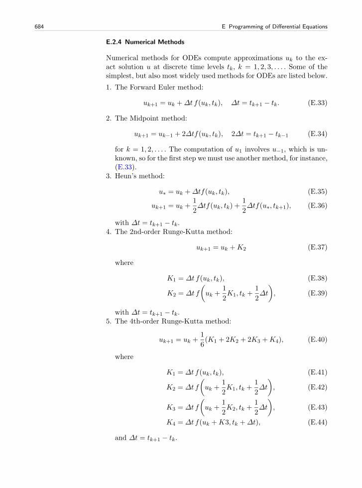
684 E Programming of Differential Equations
E.2.4 Numerical Methods
Numerical methods for ODEs compute approximations uk to the ex-act solution u at discrete time levels tk, k = 1, 2, 3, . . . . Some of thesimplest, but also most widely used methods for ODEs are listed below.
1. The Forward Euler method:
uk+1 = uk +Δt f(uk, tk), Δt = tk+1 − tk. (E.33)
2. The Midpoint method:
uk+1 = uk−1 + 2Δtf(uk, tk), 2Δt = tk+1 − tk−1 (E.34)
for k = 1, 2, . . . . The computation of u1 involves u−1, which is un-known, so for the first step we must use another method, for instance,(E.33).
3. Heun’s method:
u∗ = uk +Δtf(uk, tk), (E.35)
uk+1 = uk +1
2Δtf(uk, tk) +
1
2Δtf(u∗, tk+1), (E.36)
with Δt = tk+1 − tk.4. The 2nd-order Runge-Kutta method:
uk+1 = uk +K2 (E.37)
where
K1 = Δt f(uk, tk), (E.38)
K2 = Δt f
(uk +
1
2K1, tk +
1
2Δt
), (E.39)
with Δt = tk+1 − tk.5. The 4th-order Runge-Kutta method:
uk+1 = uk +1
6(K1 + 2K2 + 2K3 +K4), (E.40)
where
K1 = Δt f(uk, tk), (E.41)
K2 = Δt f
(uk +
1
2K1, tk +
1
2Δt
), (E.42)
K3 = Δt f
(uk +
1
2K2, tk +
1
2Δt
), (E.43)
K4 = Δt f(uk +K3, tk +Δt), (E.44)
and Δt = tk+1 − tk.

E.2 Systems of Ordinary Differential Equations 685
6. The 3rd-order Adams-Bashforth method:
uk+1 = uk +Δt
12
(23f(uk, tk)− 16f(uk−1, tk−1) + 5f(uk−2, tk−2)
),
(E.45)with Δt constant. To start the scheme, one can apply a 2nd-orderRunge-Kutta method or Heun’s method to compute u1 and u2 before(E.45) is applied for k ≥ 2.
7. The Midpoint method with iterations:
vq = uk +1
2Δt
(f(vq−1, tk+1) + f(uk, tk)
),
q = 1, . . . , N, v0 = uk (E.46)
uk+1 = vN . (E.47)
At each time level, one runs the formula (E.46) N times, and thevalue vN becomes uk+1. Setting N = 1 recovers the Forward Eulerscheme if f is independent of t, while N = 2 corresponds to Heun’smethod. We can either fix the value of N , or we can repeat (E.46)until the change in vq is small, that is, until |vq − vq−1| < ε, whereε is a small value. Fixing N is sufficient in this exercise.
8. The Backward Euler method:
uk+1 = uk +Δt f(uk+1, tk+1), Δt = tk+1 − tk. (E.48)
If f(u, t) is nonlinear in u, (E.48) constitutes a nonlinear equation inuk+1, which must be solved by some method for nonlinear equations,say Newton’s method (see Appendix E.2.6 for more details).
The methods above are valid both for scalar ODEs and for systems ofODEs. In the system case, the quantities u, uk, uk+1, f , K1, K2, etc.,are vectors.
E.2.5 The ODE Solver Class Hierarchy
Appendix E.2.3 presents a class ForwardEuler for implementing theForward Euler scheme (E.33) both for scalar ODEs and systems. Onlythe advance method should be necessary to change in order to imple-ment other numerical methods. Copying the ForwardEuler class andediting just the advance method is considered bad programming prac-tice, because we get two copies the general parts of class ForwardEuler.As we implement more schemes, we end up with a lot of copies ofthe same code. Correcting an error or improving the code in thisgeneral part then requires identical edits in several almost identicalclasses.
A good programming practice is to collect all the common code ina superclass. Subclasses can implement the advance method, but share

686 E Programming of Differential Equations
the constructor, the set_initial_condition method, and the solve
method with the superclass.
The Superclass. We introduce class ODESolver as the superclass ofvarious numerical methods for solving ODEs. Class ODESolver shouldprovide all functionality that is common to all numerical methods forODEs:
1. hold the solution u(t) at discrete time points in an array u
2. hold the corresponding time values t
3. hold information about the f(u, t) function, i.e., a callable Pythonobject f(u, t)
4. hold the current time step number k in an attribute k
5. hold the initial condition U0
6. implement the loop over all time steps
As already outlined in Appendix E.1.7, we implement the last pointas two methods: solve for performing the time loop and advance foradvancing the solution one time step. The latter method is empty in thesuperclass since the method is to be implemented by various subclassesfor various numerical schemes.
A first version class ODESolver follows directly from classForwardEuler in Appendix E.2.3, but letting advance be an emptymethod. However, there is one more extension which will be handyin some problems, namely a possibility for the user to terminate thetime loop if the solution has certain properties. Throwing a ball yieldsan example: the simulation should be stopped when the ball hitsthe ground, instead of simulating an artificial movement down in theground until the final time T is reached. To implement the requestedfeature, the user can provide a function terminate(u, t, step_no),which returns True if the time loop is be terminated. The argumentsare the solution array u, the corresponding time points t, and thecurrent time step number step_no. For example, if we want to solve anODE until the solution is (close to) zero, we can supply the function
def terminate(u, t, step_no):eps = 1.0E-6 # small numberif abs(u[step_no,0]) < eps: # close enough to zero?
return Trueelse:
return False
The terminate function is an optional argument to the solve method.By default, we provide a function that always returns False.
The suggested code for the superclass ODESolver then takes the fol-lowing form:
class ODESolver:def __init__(self, f):
self.f = lambda u, t: np.asarray(f(u, t), float)

E.2 Systems of Ordinary Differential Equations 687
def advance(self):"""Advance solution one time step."""raise NotImplementedError
def set_initial_condition(self, U0):if isinstance(U0, (float,int)): # scalar ODE
self.neq = 1U0 = float(U0)
else: # system of ODEsU0 = np.asarray(U0)self.neq = U0.size
self.U0 = U0
def solve(self, time_points, terminate=None):if terminate is None:
terminate = lambda u, t, step_no: False
self.t = np.asarray(time_points)n = self.t.sizeif self.neq == 1: # scalar ODEs
self.u = np.zeros(n)else: # systems of ODEs
self.u = np.zeros((n,self.neq))
# Assume that self.t[0] corresponds to self.U0self.u[0] = self.U0
# Time loopfor k in range(n-1):
self.k = kself.u[k+1] = self.advance()if terminate(self.u, self.t, self.k+1):
break # terminate loop over kreturn self.u[:k+2], self.t[:k+2]
Note that we return just the parts of self.u and self.t that havebeen filled with values (the rest are zeroes): all elements up to the onewith index k+1 are computed before terminate may return True. Thecorresponding slice of the array is then :k+2 since the upper limit is notincluded in the slice. If terminate never returns True we simply havethat :k+1 is the entire array.
The Forward Euler Method. Subclasses implement specific numericalformulas for numerical solution of ODEs in the advance method. Forthe Forward Euler the formula is given by (E.33). All data we need forthis formula are stored as attributes by the superclass. First we loadthese data into variables with shorter names, to avoid the lengthy self
prefix and obtain a notation closer to the mathematics. Then we applythe formula (E.33), and finally we return the new value:
class ForwardEuler(ODESolver):def advance(self):
u, f, k, t = self.u, self.f, self.k, self.tdt = t[k+1] - t[k]u_new = u[k] + dt*f(u[k], t[k])return u_new
Remark. When we extract attributes to local variables with shortnames, we should only use these local variables for reading values, not

688 E Programming of Differential Equations
setting values. For example, if we do a k += 1 to update the time stepcounter, that increased value is not reflected in self.k (which is the“official” counter). On the other hand, changing a list in-place, sayu[k+1] = ..., is reflected in self.u. Extracting class attributes in lo-cal variables is done for getting the code closer to the mathematics, buthas a danger of introducing bugs that might be hard to track down.
The 4th-order Runge-Kutta Method. Below is an implementation of the4th-order Runge-Kutta method (E.40):
class RungeKutta4(ODESolver):def advance(self):
u, f, k, t = self.u, self.f, self.k, self.tdt = t[k+1] - t[k]dt2 = dt/2.0K1 = dt*f(u[k], t[k])K2 = dt*f(u[k] + 0.5*K1, t[k] + dt2)K3 = dt*f(u[k] + 0.5*K2, t[k] + dt2)K4 = dt*f(u[k] + K3, t[k] + dt)u_new = u[k] + (1/6.0)*(K1 + 2*K2 + 2*K3 + K4)return u_new
It is left as exercises to implement other numerical methods in theODESolver class hierarchy. However, the Backward Euler method (E.48)requires a much more advanced implementation than the other methodsso that particular method deserves its own section.
E.2.6 The Backward Euler Method
The Backward Euler scheme (E.48) leads in general to a nonlinearequation at a new time level, while all the other schemes listed inAppendix E.2.4 have a simple formula for the new uk+1 value. Thenonlinear equation reads
uk+1 = uk +Δt f(uk+1, tk+1).
For simplicity we assume that the ODE is scalar so the unknown uk+1 isa scalar. It might be easier to see that the equation for uk+1 is nonlinearif we rearrange the equation to
F (w) ≡ w −Δtf(w, tk+1)− uk = 0, (E.49)
where w = uk+1. If now f(u, t) is a nonlinear function of u, F (w) willalso be a nonlinear function of w.
To solve F (w) = 0 we can use the Bisection method from Chap-ter 4.6.2, Newton’s method from Appendix A.1.10, or the Secantmethod from Exercise A.14. Here we apply Newton’s method and theimplementation given in src/diffeq/Newton.py. A disadvantage withNewton’s method is that we need the derivative of F with respect

E.2 Systems of Ordinary Differential Equations 689
to w, which requires the derivative ∂f(w, t)/∂w. A quick solution is touse a numerical derivative, e.g., class Derivative from Chapter 7.3.2.
We make a subclass BackwardEuler. As we need to solve F (w) = 0at every time step, we also need to implement the F (w) function. Thisis conveniently done in a local function inside the advance method1:
def advance(self):u, f, k, t = self.u, self.f, self.k, self.t
def F(w):return w - dt*f(w, t[k+1]) - u[k]
dFdw = Derivative(F)w_start = u[k] + dt*f(u[k], t[k]) # Forward Euler stepu_new, n, F_value = Newton(F, w_start, dFdw, N=30)if n >= 30:
print "Newton’s failed to converge at t=%g "\"(%d iterations)" % (t, n)
return u_new
The derivative dF/dw is computed numerically by a class Derivative,which is a slight modification of the similar class in Chapter 7.3.2,because we now want to use a more accurate, centered formula:
class Derivative:def __init__(self, f, h=1E-5):
self.f = fself.h = float(h)
def __call__(self, x):f, h = self.f, self.hreturn (f(x+h) - f(x-h))/(2*h)
This code is included in the ODESolver.py file after class BackwardEuler.The next step is to call Newton’s method. For this purpose we need to
import the Newton function from the Newton module. The Newton.py filemust then reside in the same directory as ODESolver.py, or Newton.py
must be in one of the directories listed in the sys.path list or thePYTHONPATH environment variable (cf. Chapter 4.5.3).
Having the Newton(f, x_start, dfdx, N) function from Ap-pendix A.1.10 accessible in our ODESolver.py file, we can make acall and supply our F function as the argument f, a start value for theiteration, here called w_start, as the argument x, and the derivativedFdw for the argument dfdx. We rely on default values for the epsilon
and store arguments, while the maximum number of iterations is setto N=30. The program is terminated if it happens that the number ofiterations exceeds that value, because then the method is not consid-ered to have converged (at least not quickly enough), and we haveconsequently not been able to compute the next uk+1 value.
1 The local variables in the advance function, e.g., dt and u, act as “global” variables forthe F function. Hence, when F is sent away to some Newton function, F remembers the values
of dt, f, t, and u!.

690 E Programming of Differential Equations
The starting value for Newton’s method must be chosen. As we ex-pect the solution to not change much from one time level to the next,uk could be a good initial guess. However, we can do better by using asimple Forward Euler step uk +Δtf(uk, tk), which is exactly what wedo in the advance function above.
Since Newton’s method always has the danger of converging slowly,it can be interesting to store the number of iterations at each time levelas an attribute in the BackwardEuler class. We can easily insert extrastatement for this purpose:
def advance(self):...u_new, n, F_value = Newton(F, w_start, dFdw, N=30)if k == 0:
self.Newton_iter = []self.Newton_iter.append(n)...
Note the need for creating an empty list (at the first call of advance)before we can append elements.
There is now one important question to ask: Will the advancemethodwork for systems of ODEs? In that case, F (w) is a vector of functions.The implementation of F will work when w is a vector, because all thequantities involved in the formula are arrays or scalar variables. ThedFdw instance will compute a numerical derivative of each componentof the vector function dFdw.f (which is simply our F function). The callto the Newton function is more critical: It turns out that this function,as the algorithm behind it, works for scalar equations only. Newton’smethod can quite easily be extended to a system of nonlinear equa-tions, but we do not consider that topic here. Instead we equip classBackwardEuler with a constructor that calls the f object and controlsthat the returned value is a float and not an array:
class BackwardEuler(ODESolver):def __init__(self, f):
ODESolver.__init__(self, f)# Make a sample call to check that f is a scalar function:try:
u = np.array([1]); t = 1value = f(u, t)
except IndexError: # index out of bounds for uraise ValueError(’f(u,t) must return float/int’)
Observe that we must explicitly call the superclass constructor andpass on the argument f to achieve the right storage and treatment ofthis argument.
Understanding class BackwardEuler implies a good understandingof classes in general; a good understanding of numerical methods forODEs, for numerical differentiation, and for finding roots of functions;and a good understanding on how to combine different code segmentsfrom different parts of the book. Therefore, if you have digested class

E.2 Systems of Ordinary Differential Equations 691
BackwardEuler, you have all reasons to believe that you have digestedthe key topics of this book.
E.2.7 Application 1: u′ = −u
The perhaps simplest of all ODEs, u′ = −u, with initial conditionu(0) = 1, is our first target problem for the classes in the ODESolver
hierarchy. The exact solution is u(t) = e−t. The basic part of the ap-plication of class ForwardEuler goes as follows:
import ODESolver
def f(u, t):return -u
solver = ODESolver.ForwardEuler(f)solver.set_initial_condition(1.0)t_points = linspace(0, 3, 31)u, t = solver.solve(t_points)plot(t, u)
We can run various values of Δt to see the effect on the accuracy:
# Test various dt values and plotfigure()T = 3for dt in 2.0, 1.0, 0.5, 0.1:
n = int(round(T/dt))solver = ODESolver.ForwardEuler(f)solver.set_initial_condition(1)u, t = solver.solve(linspace(0, T, n+1))plot(t, u, legend=’dt=%g’ % dt)hold(’on’)
plot(t, exp(-t), ’bo’, legend=’exact’)
Figure E.2 shows alarming results. With Δt = 2 we get a completelywrong solution that becomes negative and then increasing. The valueΔt = 1 gives a peculiar solution: uk = 0 for k ≥ 1! Qualitatively correctbehavior appears with Δt = 0.5, and the results get quantitativelybetter as we decrease Δt. The solution corresponding to Δ = 0.1 looksgood from the graph.
We can easily explain what we observe in Figure E.2. For the equa-tion in question, the Forward Euler method computes
u1 = u0 −Δtu0 = (1−Δt)u0,
u2 = u1 −Δtu1 = (1−Δt)u1 = (1−Δt)2u0,
...
uk = (1−Δt)ku0.
With Δt = 1 we simply get uk = 0 for k ≥ 1. For Δt > 1, 1−Δt < 0,and (1 − Δt)k means raising a negative value to an integer power,

692 E Programming of Differential Equations
Fig. E.2 Solution of u′ = −u for t ∈ [0, 3] by the Forward Euler method and
Δt ∈ {2, 1, 0.5, 0.1}.
which results in uk > 0 for even k and uk < 0 for odd k. Moreover,|uk| decreases with k. Such a growing, oscillating solution is of coursequalitatively wrong when the exact solution is e−t and monotonicallydecaying. The conclusion is that the Forward Euler method gives mean-ingless results for Δt ≥ 1 in the present example.
A particular strength of the ODESolver hierarchy of classes is thatwe can trivially switch from one method to another. For example, wemay demonstrate how superior the 4-th order Runge-Kutta method isfor this equation: just replace ForwardEuler by RungeKutta4 in the pre-vious code segment and re-run the program. It turns out that the 4-thorder Runge-Kutta method gives a monotonically decaying numericalsolution for all the tested Δt values. In particular, the solutions corre-sponding to Δt = 0.5 and Δt = 0.1 are visually very close to the exactsolution. The conclusion is that the 4-th order Runge-Kutta method isa safer and more accurate method.
Let us compare the two numerical methods in the case whereΔt = 0.5:
# Test ForwardEuler vs RungeKutta4T = 3dt = 0.5n = int(round(T/dt))t_points = linspace(0, T, n+1)figure()for solver_class in ODESolver.RungeKutta4, ODESolver.ForwardEuler:
solver = solver_class(f)solver.set_initial_condition(1)u, t = solver.solve(t_points)plot(t, u, legend=’%s’ % solver_class.__name__)hold(’on’)
plot(t, exp(-t), ’bo’, legend=’exact’)
Figure E.3 illustrates that differences in accuracy between the twomethods. The complete program can be found in the file app1_decay.py.

E.2 Systems of Ordinary Differential Equations 693
Fig. E.3 Comparison of the Forward Euler and the 4-th order Runge-Kutta method for
solving u′ = −u for t ∈ [0, 3] and a time step Δt = 0.5.
E.2.8 Application 2: The Logistic Equation
The logistic ODE (E.5) is copied here for convenience:
u′(t) = αu(t)
(1− u(t)
R
), u(0) = U0.
The right-hand side contains the parameters α and R. We know thatu → R as t → ∞, so at some point t in time we have approachedthe asymptotic value u = R within a sufficiently small tolerance andshould stop the simulation. This can be done by providing a functionas the tolerance argument in the solve method.
Basic Problem and Solver Classes. Let us, as in Appendix E.1.8, im-plement the problem-dependent data in a class. This time we store alluser-given physical data in the class:
import ODESolverfrom scitools.std import plot, figureimport numpy as np
class Problem:def __init__(self, alpha, R, U0, T):
"""alpha, R: parameters in the ODE.U0: initial condition.T: max length of time interval for integration;asymptotic value R must be reached within 1%accuracy for some t <= T."""self.alpha, self.R, self.U0, self.T = alpha, R, U0, T
def __call__(self, u, t):"""Return f(u,t) for logistic ODE."""return self.alpha*u*(1 - u/self.R)
def terminate(self, u, t, step_no):
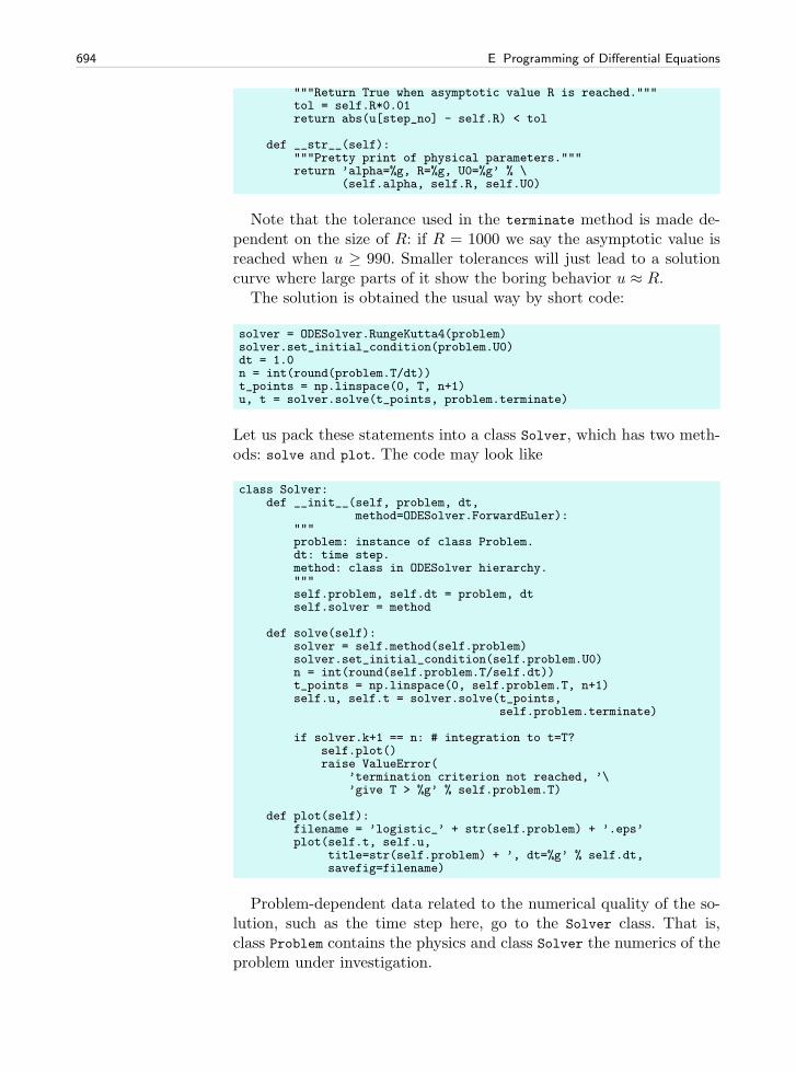
694 E Programming of Differential Equations
"""Return True when asymptotic value R is reached."""tol = self.R*0.01return abs(u[step_no] - self.R) < tol
def __str__(self):"""Pretty print of physical parameters."""return ’alpha=%g, R=%g, U0=%g’ % \
(self.alpha, self.R, self.U0)
Note that the tolerance used in the terminate method is made de-pendent on the size of R: if R = 1000 we say the asymptotic value isreached when u ≥ 990. Smaller tolerances will just lead to a solutioncurve where large parts of it show the boring behavior u ≈ R.
The solution is obtained the usual way by short code:
solver = ODESolver.RungeKutta4(problem)solver.set_initial_condition(problem.U0)dt = 1.0n = int(round(problem.T/dt))t_points = np.linspace(0, T, n+1)u, t = solver.solve(t_points, problem.terminate)
Let us pack these statements into a class Solver, which has two meth-ods: solve and plot. The code may look like
class Solver:def __init__(self, problem, dt,
method=ODESolver.ForwardEuler):"""problem: instance of class Problem.dt: time step.method: class in ODESolver hierarchy."""self.problem, self.dt = problem, dtself.solver = method
def solve(self):solver = self.method(self.problem)solver.set_initial_condition(self.problem.U0)n = int(round(self.problem.T/self.dt))t_points = np.linspace(0, self.problem.T, n+1)self.u, self.t = solver.solve(t_points,
self.problem.terminate)
if solver.k+1 == n: # integration to t=T?self.plot()raise ValueError(
’termination criterion not reached, ’\’give T > %g’ % self.problem.T)
def plot(self):filename = ’logistic_’ + str(self.problem) + ’.eps’plot(self.t, self.u,
title=str(self.problem) + ’, dt=%g’ % self.dt,savefig=filename)
Problem-dependent data related to the numerical quality of the so-lution, such as the time step here, go to the Solver class. That is,class Problem contains the physics and class Solver the numerics of theproblem under investigation.

E.2 Systems of Ordinary Differential Equations 695
If the last computed time step, solver.k+1, equals the last possibleindex, n, problem.terminate never returned True, which means that theasymptotic limit was not reached. This is treated as an erroneous con-dition. To guide the user, we launch a plot before raising the exceptionwith an instructive message. The complete code is found in the fileapp2_logistic.py.
Computing an Appropriate Δt. Choosing an appropriate Δt is not al-ways so easy. The impact of Δt can sometimes be dramatic, as demon-strated for the Forward Euler method in Appendix E.2.7. We couldautomate the process of finding a suitable Δt: start with a large Δt,and keep halving Δt until the difference between two solutions corre-sponding to two consequtive Δt values is small enough.
Say solver is a class Solver instance computed with time step Δtand solver2 is the instance corresponding to a computation with Δt/2.Calculating at the difference between solver.u and solver2.u is nottrivial as (i) one of the arrays has approximately twice as many elementsas the other, and (ii) the last element in both arrays does not necessarilycorrespond to the same time value since the time stepping and theterminate function may lead to slightly different termination times.
A solution to these two problems is to turn each of the arrayssolver.u and solver2.u into continuous functions, as explained in Ap-pendix E.1.5, and then evaluate the difference at some selected timepoints up to the smallest value of solver.t[-1] and solver2.t[-1].The code becomes
# Make continuous functions u(t) and u2(t)u = wrap2callable((solver. t, solver. u))u2 = wrap2callable((solver2.t, solver2.u))# Sample the difference in n points in [0, t_end]n = 13t_end = min(solver2.t[-1], solver.t[-1])t = np.linspace(0, t_end, n)u_diff = np.abs(u(t) - u2(t)).max()
The next step is to introduce a loop where we halve the time step ineach iteration and solve the logistic ODE with the new time step andcompute u_diff as shown above. A complete function takes the form
def find_dt(problem, method=ODESolver.ForwardEuler,tol=0.01, dt_min=1E-6):
"""Return a "solved" class Solver instance where thedifference in the solution and one with a doubletime step is less than tol.
problem: class Problem instance.method: class in ODESolver hierarchy.tol: tolerance (chosen relative to problem.R).dt_min: minimum allowed time step."""dt = problem.T/10 # start with 10 intervalssolver = Solver(problem, dt, method)
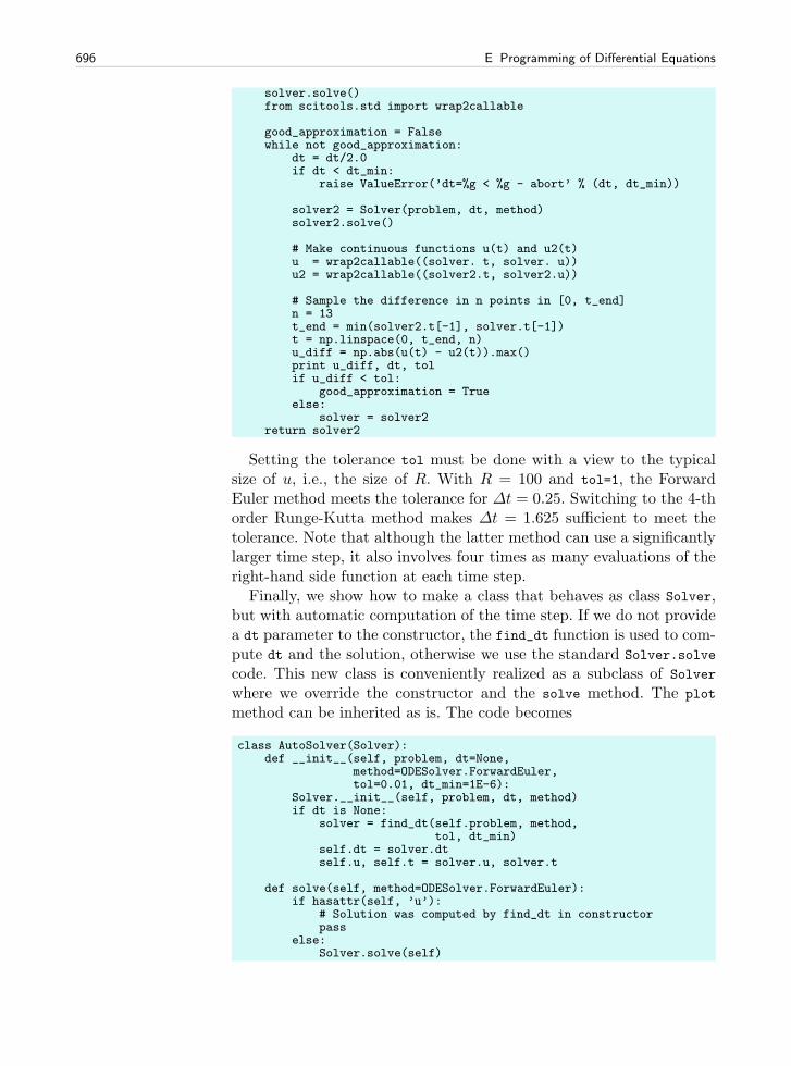
696 E Programming of Differential Equations
solver.solve()from scitools.std import wrap2callable
good_approximation = Falsewhile not good_approximation:
dt = dt/2.0if dt < dt_min:
raise ValueError(’dt=%g < %g - abort’ % (dt, dt_min))
solver2 = Solver(problem, dt, method)solver2.solve()
# Make continuous functions u(t) and u2(t)u = wrap2callable((solver. t, solver. u))u2 = wrap2callable((solver2.t, solver2.u))
# Sample the difference in n points in [0, t_end]n = 13t_end = min(solver2.t[-1], solver.t[-1])t = np.linspace(0, t_end, n)u_diff = np.abs(u(t) - u2(t)).max()print u_diff, dt, tolif u_diff < tol:
good_approximation = Trueelse:
solver = solver2return solver2
Setting the tolerance tol must be done with a view to the typicalsize of u, i.e., the size of R. With R = 100 and tol=1, the ForwardEuler method meets the tolerance for Δt = 0.25. Switching to the 4-thorder Runge-Kutta method makes Δt = 1.625 sufficient to meet thetolerance. Note that although the latter method can use a significantlylarger time step, it also involves four times as many evaluations of theright-hand side function at each time step.
Finally, we show how to make a class that behaves as class Solver,but with automatic computation of the time step. If we do not providea dt parameter to the constructor, the find_dt function is used to com-pute dt and the solution, otherwise we use the standard Solver.solve
code. This new class is conveniently realized as a subclass of Solver
where we override the constructor and the solve method. The plot
method can be inherited as is. The code becomes
class AutoSolver(Solver):def __init__(self, problem, dt=None,
method=ODESolver.ForwardEuler,tol=0.01, dt_min=1E-6):
Solver.__init__(self, problem, dt, method)if dt is None:
solver = find_dt(self.problem, method,tol, dt_min)
self.dt = solver.dtself.u, self.t = solver.u, solver.t
def solve(self, method=ODESolver.ForwardEuler):if hasattr(self, ’u’):
# Solution was computed by find_dt in constructorpass
else:Solver.solve(self)

E.2 Systems of Ordinary Differential Equations 697
The call hasattr(self,’u’) returns True if u is an attribute in objectself. Here this is used as an indicator that the solution was computedin the constructor by the find_dt function. A typical use is
problem = Problem(alpha=0.1, R=500, U0=2, T=130)solver = AutoSolver(problem, tol=1)solver.solve(method=ODESolver.RungeKutta4)solver.plot()
Dealing with Time-Dependent Coefficients. The carrying capacity ofthe environment, R, may vary with time, e.g., due to seasonal changes.Can we extend the previous code so that R can be specified either asa constant or as a function of time?
This is in fact easy if we in the implementation of the right-hand sidefunction assume that R is a function of time. If it is given as a constantin the constructor of class Problem, we just wrap it as a function oftime:
if isinstance(R, (float,int)): # number?self.R = lambda t: R
elif callable(R):self.R = R
else:raise TypeError(
’R is %s, has to be number of function’ % type(R))
The terminate method is also affected as we need to base the toleranceon the R value at the present time level. Also the __str__ method mustbe changed since it is not meaningful to print a function self.R. Thatis, all methods in the generalized problem class, here called Problem2,must be altered. We have not chosen to make Problem2 a subclass ofProblem, even though the interface is the same and the two classes areclosely related. While Problem is clearly a special case of Problem2, asa constant R is a special case of a function (R), the opposite case isnot true.
Class Problem2 becomes
class Problem2(Problem):def __init__(self, alpha, R, U0, T):
"""alpha, R: parameters in the ODE.U0: initial condition.T: max length of time interval for integration;asymptotic value R must be reached within 1%accuracy for some t <= T."""self.alpha, self.U0, self.T = alpha, U0, Tif isinstance(R, (float,int)): # number?
self.R = lambda t: Relif callable(R):
self.R = Relse:
raise TypeError(’R is %s, has to be number of function’ % type(R))
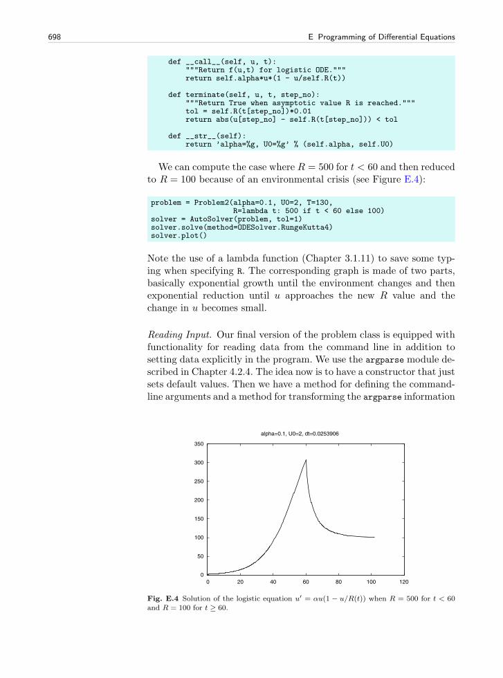
698 E Programming of Differential Equations
def __call__(self, u, t):"""Return f(u,t) for logistic ODE."""return self.alpha*u*(1 - u/self.R(t))
def terminate(self, u, t, step_no):"""Return True when asymptotic value R is reached."""tol = self.R(t[step_no])*0.01return abs(u[step_no] - self.R(t[step_no])) < tol
def __str__(self):return ’alpha=%g, U0=%g’ % (self.alpha, self.U0)
We can compute the case where R = 500 for t < 60 and then reducedto R = 100 because of an environmental crisis (see Figure E.4):
problem = Problem2(alpha=0.1, U0=2, T=130,R=lambda t: 500 if t < 60 else 100)
solver = AutoSolver(problem, tol=1)solver.solve(method=ODESolver.RungeKutta4)solver.plot()
Note the use of a lambda function (Chapter 3.1.11) to save some typ-ing when specifying R. The corresponding graph is made of two parts,basically exponential growth until the environment changes and thenexponential reduction until u approaches the new R value and thechange in u becomes small.
Reading Input. Our final version of the problem class is equipped withfunctionality for reading data from the command line in addition tosetting data explicitly in the program. We use the argparse module de-scribed in Chapter 4.2.4. The idea now is to have a constructor that justsets default values. Then we have a method for defining the command-line arguments and a method for transforming the argparse information
Fig. E.4 Solution of the logistic equation u′ = αu(1 − u/R(t)) when R = 500 for t < 60
and R = 100 for t ≥ 60.

E.2 Systems of Ordinary Differential Equations 699
to the attributes alpha, U0, R, and T. The R attribute is supposed to bea function, and we use the StringFunction tool to turn strings fromthe command-line into a Python function of time t.
The code of our new problem class is listed next.
class Problem3(Problem):def __init__(self):
# Set default parameter valuesself.alpha = 1.self.R = StringFunction(’1.0’, independent_variable=’t’)self.U0 = 0.01self.T = 4.
def define_command_line_arguments(self, parser):"""Add arguments to parser (argparse.ArgumentParser)."""
def evalcmlarg(text):return eval(text)
def toStringFunction(text):return StringFunction(text, independent_variable=’t’)
parser.add_argument(’--alpha’, dest=’alpha’, type=evalcmlarg,default=self.alpha,help=’initial growth rate in logistic model’)
parser.add_argument(’--R’, dest=’R’, type=toStringFunction, default=self.R,help=’carrying capacity of the environment’)
parser.add_argument(’--U0’, dest=’U0’, type=evalcmlarg, default=self.U0,help=’initial condition’)
parser.add_argument(’--T’, dest=’T’, type=evalcmlarg, default=self.T,help=’integration in time interval [0,T]’)
return parser
def set(self, **kwargs):"""Set parameters as keyword arguments alpha, R, U0, or T,or as args (object returned by parser.parse_args())."""for prm in (’alpha’, ’U0’, ’R’, ’T’):
if prm in kwargs:setattr(self, prm, kwargs[prm])
if ’args’ in kwargs:args = kwargs[’args’]for prm in (’alpha’, ’U0’, ’R’, ’T’):
if hasattr(args, prm):setattr(self, prm, getattr(args, prm))
else:print ’Really strange’, dir(args)
def __call__(self, u, t):"""Return f(u,t) for logistic ODE."""return self.alpha*u*(1 - u/self.R(t))
def terminate(self, u, t, step_no):"""Return True when asymptotic value R is reached."""tol = self.R(t[step_no])*0.01return abs(u[step_no] - self.R(t[step_no])) < tol
def __str__(self):s = ’alpha=%g, U0=%g’ % (self.alpha, self.U0)if isinstance(self.R, StringFunction):
700 E Programming of Differential Equations
s += ’, R=%s’ % str(self.R)return s
The calls to parser.add_argument are straightforward, but noticethat we allow strings for α, U0, and T to be interpreted by eval. Thestring for R is interpreted as a formula by StringFunction. The set
method is flexible: it accepts any set of keyword arguments, and checksfirst if these are the names of the problem parameters, and thereafter ifargs=’ is given, which implies that the parameters are taken from thecommand line. The rest of the class is very similar to earlier versions.
The typical use of class Problem3 is shown below. First we set pa-rameters directly:
problem = Problem3()problem.set(alpha=0.1, U0=2, T=130,
R=lambda t: 500 if t < 60 else 100)solver = AutoSolver(problem, tol=1)solver.solve(method=ODESolver.RungeKutta4)solver.plot()
Then we rely on reading parameters from the command line:
problem = Problem3()import argparseparser = argparse.ArgumentParser(
description=’Logistic ODE model’)parser = problem.define_command_line_arguments(parser)
# Try --alpha 0.11 --T 130 --U0 2 --R ’500 if t < 60 else 300’args = parser.parse_args()problem.set(args=args)solver = AutoSolver(problem, tol=1)solver.solve(method=ODESolver.RungeKutta4)solver.plot()
The last example using a problem class integrated with the commandline is the most flexible way of implementing ODE models.
E.2.9 Application 3: An Oscillating System
The motion of a box attached to a spring, as described in Appendix D,can be modeled by two first-order differential equations as listed in(E.32), here repeated with F (t) = mw′′(t) for convenience:
du(0)
dt= u(1),
du(1)
dt= w′′(t) + g −m−1βu(1) −m−1ku(0).
The w(t) function is the forced movement of the end of the spring.The code related to this example is found in app3_osc.py. Because
our right-hand side f contains several parameters, we implement it as

E.2 Systems of Ordinary Differential Equations 701
a class with the parameters as attributes and a __call__ method forreturning the 2-vector f . We assume that the user of the class suppliesthe w(t) function, so it is natural to compute w′′(t) by a finite differenceformula.
class OscSystem:def __init__(self, m, beta, k, g, w):
self.m, self.beta, self.k, self.g, self.w = \float(m), float(beta), float(k), float(g), w
def __call__(self, u, t):u0, u1 = um, beta, k, g, w = \
self.m, self.beta, self.k, self.g, self.w# Use a finite difference for w’’(t)h = 1E-5ddw = (w(t+h) - 2*w(t) + w(t-h))/(h**2)f = [u1, ddw + g - beta/m*u1 - k/m*u0]return f
A simple test case arises if we set m = k = 1 and β = g = w = 0:
du(0)
dt= u(1),
du(1)
dt= −u(0).
Suppose that u(0)(0) = 1 and u(1)(0) = 0. An exact solution is then
u(0)(t) = cos t, u(1)(t) = − sin t.
We can use this case to check how the Forward Euler method compareswith the 4-th order Runge-Kutta method:
import ODESolverfrom scitools.std import *f = OscSystem(1.0, 0.0, 1.0, 0.0, lambda t: 0)u_init = [1, 0] # initial conditionnperiods = 3.5 # no of oscillation periodsT = 2*pi*nperiodsfor solver_class in ODESolver.ForwardEuler, ODESolver.RungeKutta4:
if solver_class == ODESolver.ForwardEuler:npoints_per_period = 200
elif solver_class == ODESolver.RungeKutta4:npoints_per_period = 20
n = npoints_per_period*nperiodst_points = linspace(0, T, n+1)solver = solver_class(f)solver.set_initial_condition(u_init)u, t = solver.solve(t_points)
# u is an array of [u0,u1] pairs for each time level,# get the u0 values from u for plottingu0_values = u[:, 0]u1_values = u[:, 1]u0_exact = cos(t)u1_exact = -sin(t)figure()alg = solver_class.__name__ # (class) name of algorithmplot(t, u0_values, ’r-’,
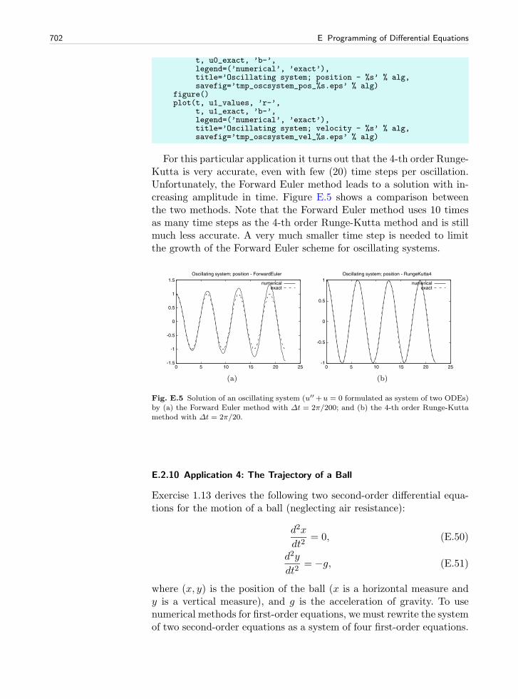
702 E Programming of Differential Equations
t, u0_exact, ’b-’,legend=(’numerical’, ’exact’),title=’Oscillating system; position - %s’ % alg,savefig=’tmp_oscsystem_pos_%s.eps’ % alg)
figure()plot(t, u1_values, ’r-’,
t, u1_exact, ’b-’,legend=(’numerical’, ’exact’),title=’Oscillating system; velocity - %s’ % alg,savefig=’tmp_oscsystem_vel_%s.eps’ % alg)
For this particular application it turns out that the 4-th order Runge-Kutta is very accurate, even with few (20) time steps per oscillation.Unfortunately, the Forward Euler method leads to a solution with in-creasing amplitude in time. Figure E.5 shows a comparison betweenthe two methods. Note that the Forward Euler method uses 10 timesas many time steps as the 4-th order Runge-Kutta method and is stillmuch less accurate. A very much smaller time step is needed to limitthe growth of the Forward Euler scheme for oscillating systems.
Fig. E.5 Solution of an oscillating system (u′′+u = 0 formulated as system of two ODEs)by (a) the Forward Euler method with Δt = 2π/200; and (b) the 4-th order Runge-Kutta
method with Δt = 2π/20.
E.2.10 Application 4: The Trajectory of a Ball
Exercise 1.13 derives the following two second-order differential equa-tions for the motion of a ball (neglecting air resistance):
d2x
dt2= 0, (E.50)
d2y
dt2= −g, (E.51)
where (x, y) is the position of the ball (x is a horizontal measure andy is a vertical measure), and g is the acceleration of gravity. To usenumerical methods for first-order equations, we must rewrite the systemof two second-order equations as a system of four first-order equations.

E.2 Systems of Ordinary Differential Equations 703
This is done by introducing to new unknowns, the velocities vx = dx/dtand vy = dy/dt. We then have the first-order system of ODEs
dx
dt= vx, (E.52)
dvxdt
= 0, (E.53)
dy
dt= vy, (E.54)
dvydt
= −g. (E.55)
The initial conditions are
x(0) = 0, (E.56)
vx(0) = v0 cos θ, (E.57)
y(0) = y0, (E.58)
vy(0) = v0 sin θ, (E.59)
where v0 is the initial magnitude of the velocity of the ball. The initialvelocity has a direction that makes the angle θ with the horizontal.
The code related to this example is found in app4_ball.py. A func-tion returning the right-hand side of our ODE system reads
def f(u, t):x, vx, y, vy = ug = 9.81return [vx, 0, vy, -g]
It makes sense to solve the ODE system as long as the ball as above theground, i.e., as long as y ≥ 0. We must therefore supply a terminate
function as explained on page 686:
def terminate(u, t, step_no):return False if u[step_no,2] >= 0 else True
Observe that all the y values are given by u[:,2] and we want to testthe value at the current step, which becomes u[step_no,2].
The main program for solving the ODEs can be set up as
v0 = 5theta = 80*pi/180U0 = [0, v0*cos(theta), 0, v0*sin(theta)]T = 1.2; dt = 0.01; n = int(round(T/dt))solver = ODESolver.ForwardEuler(f)solver.set_initial_condition(U0)
def terminate(u, t, step_no):return False if u[step_no,2] >= 0 else True
u, t = solver.solve(linspace(0, T, n+1), terminate)

704 E Programming of Differential Equations
Now, u[:,0] represents all the x(t) values, u[:,1] all the vx(t) values,u[:,2] all the y(t) values, and u[:,3] all the vy(t) values. To plot thetrajectory, y versus x, we write
x = u[:,0]y = u[:,2]plot(x, y)
The exact solution is given by (1.5), so we can easily assess the accu-racy of the numerical solution. Figure E.6 shows a comparison of thenumerical and the exact solution in this simple test problem. Note thateven if we are just interested in y as a function of x, we first need tosolve the complete ODE system for x(t), vx(t), y(t), and vy(t).
The real strength of the numerical approach is the ease with which wecan add air resistance and lift to the system of ODEs. Insight in physicsis necessary to derive what the additional terms are, but implementingthe terms is trivial in our program above (do Exercise E.32).
Fig. E.6 The trajectory of a ball solved as a system of four ODEs by the Forward Eulermethod.
E.2.11 Further Developments of ODESolver
The ODESolver hierarchy is a simplified prototype version of a more pro-fessional Python package for solving ODEs called Odespy. This packagefeatures a range of simple and sophisticated methods for solving scalarODEs and systems of ODEs. Some of the solvers are implemented inPython, while others call up well-known ODE software in Fortran. Likethe ODESolver hierarchy, Odespy offers a unified interface to the differ-ent numerical methods, which means that the user can specify the ODEproblem as a function f(u,t) and send this function to all solvers. This

E.3 Exercises 705
feature makes it easy to switch between solvers to test a wide collectionof numerical methods for a problem.
Odespy can be downloaded from http://hplgit.github.com/odespy/.It is installed by the usual python setup.py install command.
E.3 Exercises
Exercise E.1. Solve a simple ODE in two ways.The purpose of this exercise is to solve the ODE problem u−10u′ = 0,
u(0) = 0.2, for t ∈ [0, 20]. Use both the ForwardEuler function fromAppendix E.1.3 and the ForwardEuler class from Appendix E.1.7. SetΔt = 1. Check that the results produced by the two equivalent methodscoincide. Name of program file: simple_ODE.py. �
Exercise E.2. Use the ODESolver hierarchy to solve a simple ODE.Solve the ODE problem u′ = u/2 with u(0) = 1, using a class in
the ODESolver hierarchy. Choose Δt = 0.5 and find u(t) for t ∈ [0, 6].Write out the approximate final un value together with the exactvalue e3. Repeat the calculations for Δt = 0.001. Name of programfile: ODESolver_demo.py. �
Exercise E.3. Solve an ODE for emptying a tank.A cylindrical tank of radius R is filled with water to a height h0. By
opening a valve of radius r at the bottom of the tank, water flows out,and the height of water, h(t), decreases with time. We can derive anODE that governs the height function h(t).
Mass conservation of water requires that the reduction in heightbalances the outflow. In a time interval Δt, the height is reduced byΔh, which corresponds to a water volume of πR2Δh. The water leavingthe tank in the same interval of time equals πr2vΔt, where v is theoutflow velocity. It can be shown (from what is known as Bernoulli’sequation) that
v(t) =√
2gh(t) + h′(t)2,
g being the acceleration of gravity [6, 11]. Note that Δh > 0 impliesan increase in h, which means that −πR2Δh is the corresponding de-crease in volume that must balance the outflow loss of volume πr2vΔt.Elimination of v and taking the limit Δt → 0 lead to the ODE
dh
dt= −
(r
R
)2(1−
(r
R
)4)−1/2√2gh.
For practical applications r � R so that 1− (r/R)4 ≈ 1 is a reasonableapproximation (friction is neglected in the derivation, and we are alsogoing to solve the ODE by approximate methods). The final ODE then

706 E Programming of Differential Equations
becomesdh
dt= −
(r
R
)2√2gh. (E.60)
The initial condition follows from the initial height of water, h0, in thetank: h(0) = h0.
Solve (E.60) by a numerical method of your choice in a program. Setr = 1 cm, R = 20 cm, g = 9.81 m/s2, and h0 = 1 m. Use a time stepof 10 seconds. Plot the solution, and experiment to see what a propertime interval for the simulation is. Make sure to test for h < 0 so thatyou do not apply the square root function to negative numbers. Canyou find an analytical solution of the problem to compare the numericalsolution with? Name of program file: tank_ODE.py. �
Exercise E.4. Scale the logistic equation.Consider the logistic model (E.5):
u′(t) = αu(t)
(1− u(t)
R
), u(0) = U0.
This problem involves three input parameters: U0, R, and α. Learninghow u varies with U0, R, and α requires much experimentation wherewe vary all three parameters and observe the solution. A much moreeffective approach is to scale the problem. By this technique the solu-tion depends only on one parameter U0/R in the present problem. Thisexercise tells how the scaling is done.
The idea of scaling is to introduce dimensionless versions of theindependent and dependent variables:
v =u
uc, τ =
t
tc,
where uc and tc are characteristic sizes of u and t, respectively, suchthat the dimensionless variables v and τ are of approximately unitsize. Since we know that u → R as t → ∞, R can be taken as thecharacteristic size of u.
Insert u = Rv and t = tcτ in the governing ODE and choose tc =1/α. Show that the ODE for the new function v(τ) becomes
dv
dτ= v(1− v), v(0) = v0. (E.61)
We see that the three parameters U0, R, and α have disappeared fromthe ODE problem, and only one parameter v0 = U0/R is involved.
Show that if v(τ) is computed, one can recover u(t) by
u(t) = Rv(αt). (E.62)
Geometrically, the transformation from v to u is just a stretching ofthe two axis in the coordinate system.

E.3 Exercises 707
Make a program logistic_scaled.py where you compute v(τ), givenv0 = 0.05, and then you use (E.62) to plot u(t) for R = 100, 500, 1000and α = 1 in one figure, and u(t) for α = 1, 5, 10 and R = 1000in another figure. Note how effectively you can generate u(t) withoutneeding to solve an ODE problem, and also note how varying R and αimpacts the graph of u(t). Name of program file: logistic_scaled.py.�
Exercise E.5. Compute logistic growth with time-varying carrying ca-pacity.
Use classes Problem2 and AutoSolver from Appendix E.2.8 to studylogistic growth when the carrying capacity of the environment, R,changes periodically with time: R = 500 for its ≤ t < (i + 1)ts andR = 200 for (i + 1)ts ≤ t < (i + 2)ts, with i = 0, 2, 4, 6, . . . . Usethe same data as in Appendix E.2.8, and find some relevant sizes ofthe period of variation, ts, to experiment with. Name of program file:seasonal_logistic_growth.py. �
Exercise E.6. Solve an ODE for the arc length.Given a curve y = f(x), the length of the curve from x = x0 to some
point x is given by the function s(x), which solves the problem
ds
dx=
√1 +
[f ′(x)
]2, s(x0) = 0. (E.63)
Since s does not enter the right-hand side, (E.63) can immediatelybe integrated from x0 to x (see Exercise A.17). However, we shallsolve (E.63) as an ODE. Use the Forward Euler method and com-pute the length of a straight line (for easy verification) and a parabola:f(x) = 1
2x + 1, x ∈ [0, 2]; f(x) = x2, x ∈ [0, 2]. Name of program file:arclength_ODE.py. �
Exercise E.7. Compute inverse functions by solving an ODE.The inverse function g of some function f(x) takes the value f(x)
back to x again: g(f(x)) = x. The common technique to computeinverse functions is to set y = f(x) and solve with respect to x. Theformula on the right-hand side is then the desired inverse function g(y).Exercise 7.26 makes use of such an approach, where y − f(x) = 0 issolved numerically with respect to x for different discrete values of y.
We can formulate a general procedure for computing inverse func-tions from an ODE problem. If we differentiate y = f(x) with respectto y, we get 1 = f ′(x)dxdy by the chain rule. The inverse function we
seek is x(y), but this function then fulfills the ODE
x′(y) =1
f ′(x). (E.64)

708 E Programming of Differential Equations
That y is the independent coordinate and x the function of y can bea somewhat confusing notation, so you might introduce u and t for xand y:
u′(t) =1
f ′(u).
The initial condition is x(0) = xr where xr solves the equationf(xr) = 0 (x(0) implies y = 0 and then from y = f(x) it followsthat f(x(0)) = 0).
Make a program that can use the described method to compute x(y),given f(x) and xr. Use any numerical method of your choice for solvingthe ODE problem. Plot f(x) as well as x(y). Verify the implementationfor f(x) = 2x. Test the method for f(x) =
√x. Name of program file:
inverse_ODE.py. �
Exercise E.8. Generalize the implementation in Exer. E.7.The method for computing inverse functions described in Exer-
cise E.7 is very general. The purpose now is to make a reusable utility,here called Inverse, for computing the inverse of some Python functionf(x) on some interval I=[a,b]. The utility can be used as follows tocalculate the inverse of sinx on I = [0, π/2]:
def f(x):return sin(x)
# Compute the inverse of finverse = Inverse(f, x0=0, I=[0, pi/2], resolution=100)x, y = Inverse.compute()from scitools.std import plot
plot(y, x, ’r-’,x, f(x), ’b-’,y, asin(y), ’go’)
legend([’computed inverse’, ’f(x)’, ’exact inverse’])
Here, x0 is the value of x at 0, or in general at the left point of theinterval: I[0]. The parameter resolution tells how many equally sizedintervals Δy we use in the numerical integration of the ODE. A defaultchoice of 1000 can be used if it is not given by the user.
Make class Inverse and put it in a module. Include a function_verify() in the module which tests that class Inverse gives exact solu-tion for the test problem f(x) = 2x. Name of program file: Inverse1.py.�
Exercise E.9. Extend the implementation in Exer. E.8.Extend the module in Exercise E.8 such that the value of x(0) (x0
in class Inverse’s constructor) does not need to be provided by theuser. To this end, class Inverse must solve f(x) = 0 and set x0 equalto the root. You may use the Bisection method from Chapter 4.6.2,Newton’s method from Appendix A.1.10, or the Secant method fromExercise A.14 to solve f(x) = 0. Class Inverse should figure out a

E.3 Exercises 709
suitable initial interval for the Bisection method or start values for theNewton or Secant methods. Computing f(x) for x at many points andexamining these may help in solving f(x) = 0 without any input fromthe user. Name of program file: Inverse2.py. �
Exercise E.10. Compute inverse functions by interpolation.Instead of solving an ODE for computing the inverse function g(y) of
some function f(x), as explained in Exercise E.7, one may use a simplerapproach based on ideas from Appendix E.1.5. Say we compute discretevalues of x and f(x), stored in the arrays x and y. Doing a plot(x, y)
shows y = f(x) as a function of x, and doing plot(y, x) shows x asa function of y, i.e., we plot the inverse function g(y). It is thereforetrivial to plot the inverse function!
However, if we want the inverse function of f(x) as some Pythonfunction g(y) that we can call for any y, we can use the toolwrap2callable from Appendix E.1.5 to turn the discrete inverse func-tion, described by the arrays y (independent coordinate) and x (depen-dent coordinate), into a continuous function g(y):
from scitools.std import wrap2callableg = wrap2callable((y, x))
y = 0.5print g(y)
The g(y) function applies linear interpolation in each interval betweenthe points in the y array.
Implement this method in a program. Verify the implementation forf(x) = 2x for x ∈ [0, 4] and test it for f(x) = sinx for x ∈ [0, π/2].Name of program file: inverse_wrap2callable.py. �
Exercise E.11. Simulate a falling or rising body in a fluid.A body moving vertically through a fluid (liquid or gas) is subject
to three different types of forces:
1. the gravity force Fg = −mg, where m is the mass of the body and gis the acceleration of gravity;
2. the drag force2 Fd = −12CD�A|v|v (see also Exercise 1.11), where CD
is a dimensionless drag coefficient depending on the body’s shape,� is the density of the fluid, A is the cross-sectional area (producedby a cutting plane y = const through the thickest part of the body),and v is the velocity;
3. the uplift or buoyancy force (“Archimedes force”) Fb = �gV , whereV is the volume of the body.
2 Roughly speaking, the Fd formula is suitable for medium to high velocities, while for verysmall velocities, or very small bodies, Fd is proportional to the velocity, not the velocity
squared, see [11].

710 E Programming of Differential Equations
Newton’s second law applied to the body says that the sum of theseforces must equal the mass of the body times its acceleration a:
Fg + Fd + Fb = ma,
which gives
−mg − 1
2CD�A|v|v + �gV = ma.
The unknowns here are v and a, i.e., we have two unknowns but onlyone equation. From kinematics in physics we know that the accelerationis the time derivative of the velocity: a = dv/dt. This is our secondequation. We can easily eliminate a and get a single differential equationfor v:
−mg − 1
2CD�A|v|v + �gV = m
dv
dt.
A small rewrite of this equation is handy: We express m as �bV , where�b is the density of the body, and we isolate dv/dt on the left-hand side,
dv
dt= −g
(1− �
�b
)− 1
2CD
�A
�bV|v|v. (E.65)
This differential equation must be accompanied by an initial condition:v(0) = V0.
Make a program for solving (E.65) numerically, using any numericalmethod of your choice. Implement the right-hand side of (E.65) in the__call__ method of a class where the parameters g, �, �b, CD, A, andV are attributes.
To verify the program, assume a heavy body in air such that the Fb
force can be neglected, and assume a small velocity such that the airresistance Fd can also be neglected. Setting � = 0 removes both theseterms from the equation. The motion then leads to the exact velocityv(t) = y′(t) = v0−gt. See how well the program reproduces this simplesolution.
After the program is verified, we are ready to run two real examplesand plot the evolution of v:
1. Parachute jumper. The point is to compute the motion of a parachutejumper in free fall before the parachute opens. We set the density ofthe human body as �b = 1003 kg/m3 and the mass as m = 80 kg,implying V = m/�b = 0.08 m3. We can base the cross-sectional areaA on the height 1.8 m and a width of 50 cm, giving A ≈ πR2 =0.9 m2. The density of air decreases with height, and we here use thevalue 0.79 kg/m3 which is relevant for about 5000 m height. The CD
coefficient can be set as 0.6. Start with v0 = 0.2. Rising ball in water. A ball with the size of a soccer ball is placed in
deep water, and we seek to model its motion upwards. Contrary to

E.3 Exercises 711
the former example, where the buoyancy force Fb is very small, Fb isnow the driving force, and the gravity force Fg is small. Set A = πa2
with a = 11 cm, the mass of the ball is 0.43 kg, the density of wateris 1000 kg/m3, and CD is 0.2. Start with v0 = 0 and see how the ballrises.
Name of program file: body_in_fluid.py. �
Exercise E.12. Check the solution’s limit in Exer. E.11.The solution of (E.65) often tends to a constant velocity, called the
terminal velocity. This happens when the sum of the forces, i.e., theright-hand side in (E.65) vanishes. Compute the formula for the ter-minal velocity by hand. Solve the ODE using class ODESolver andcall the solve method with a terminate function that terminatesthe computations when a constant velocity is reached, that is, when|v(tn) − v(tn−1)| ≤ ε, where ε is a small number. Run a series of Δtvalues and make a graph of the terminal velocity as a function of Δtfor the two cases in Exercise E.11. Indicate the exact terminal velocityin the plot by a horizontal line. Would you expect the accuracy of thecomputed terminal velocity to increase with decreasing Δt? Discuss!Name of program file: body_in_fluid_termvel.py. �
Exercise E.13. Visualize the different forces in Exer. E.11.The purpose of this exercise is to plot the forces Fg, Fb, and Fd in the
model from Exercise E.11 as functions of t. Seeing the relative impor-tance of the forces as time develops gives an increased understandingof how the different forces contribute to change the velocity. Name ofprogram file: body_in_fluid_forces.py. �
Exercise E.14. Solve an ODE until constant solution.Newton’s law of cooling,
dT
dt= −h(T − Ts) (E.66)
can be used to see how the temperature T of an object changes be-cause of heat exchange with the surroundings, which have a tempera-ture Ts. The parameter h, with unit s−1 is an experimental constant(heat transfer coefficient) telling how efficient the heat exchange withthe surroundings is. For example, (E.66) may model the cooling of ahot pizza taken out of the oven. The problem with applying (E.66),nevertheless, is that h must be measured. Suppose we have measuredT at t = 0 and t1. We can use a rough Forward Euler approximationof (E.66) with one time step of length t1,
T (t1)− T (0)
t1= −h
(T (0)− Ts
),
to make the estimate

712 E Programming of Differential Equations
h =T (t1)− T (0)
t1(Ts − T (0)). (E.67)
Suppose now you take a hot pizza out of the oven. The temperatureof the pizza is 200 C at t = 0 and 180 C after 50 seconds, in a roomwith temperature 20 C. Find an estimate of h from the formula above.
Solve (E.66) to find the evolution of the temperature of the pizza. Useclass ForwardEuler or RungeKutta4, and supply a terminate function tothe solve method so that the simulation stops when T is sufficientlyclose to the final room temperature Ts. Plot the solution. Name ofprogram file: pizza_cooling1.py. �
Exercise E.15. Use classes in Exer. E.14.Solve Exercise E.14 with a class Problem containing the parameters
h, Ts, T (0), and Δt as attributes. A method estimate_h should taket1 and T (t1) as arguments, compute h, and assign it to self.h. Also amethod __call__ for computing the right-hand side must be included.The terminate function can be a method in the class, a stand-alonefunction, or a lambda function. By using class Problem, we avoid havingthe physical parameters as global variables in the program and all theproblem-specific data are packed into one object.
Write a function solve(problem) that takes a Problem object withname problem as argument, solves the ODE, and plots the solution. Wenow want to run experiments with different values of some parameters:Ts = 15, 22, 30 C and T (0) = 250, 200 C. Make a list of Problem objectsand plot the solution for each problem in the same figure:
# Given h and dtproblems = [Problem(h, T_s, T_0, dt) \
for T_s in 15, 22, 30 for T_0 in 250, 200]for problem in problems:
solve(problem)hold(’on’)
Name of program file: pizza_cooling2.py. �
Exercise E.16. Scale away parameters in Exer. E.14.Use the scaling approach from Appendix E.2.8 to “scale away” the
parameters in the ODE in Exercise E.14. That is, introduce a newunknown u = (T − Ts)/(T (0)− Ts) and a new time scale τ = th. Findthe ODE and the initial condition that governs the u(τ) function. Makea program that computes u(τ) until |u| < 0.001. Store the discreteu and τ values in a file u_tau.dat if that file is not already present(you can use os.path.isfile(f) to test if a file with name f exists).Create a function T(u, tau, h, T0, Ts) that loads the u and τ datafrom the u_tau.dat file and returns two arrays with T and t values,corresponding to the computed arrays for u and τ . Plot T versus t.Give the parameters h, Ts, and T (0) on the command line. Note thatthis program is supposed to solve the ODE once and then recover any

E.3 Exercises 713
T (t) solution by a simple scaling of the single u(τ) solution. Name ofprogram file: pizza_cooling3.py. �
Exercise E.17. Use the 4th-order Runge-Kutta on (C.34).Investigate if the 4th-order Runge-Kutta method is better than the
Forward Euler scheme for solving the challenging ODE problem (C.34)from Exercise C.3 on page 639. Name of program file: yx_ODE2.py. �
Exercise E.18. Compare ODE methods.The equation u′ = −au is a relevant model for radioactive decay,
where u(t) is the fraction of particles that remains in the radioactivesubstance at time t. The parameter a is the inverse of the so-calledmean lifetime of the substance. The initial condition is u(0) = 1.
Introduce a class Decay to hold information about the physical prob-lem: the parameter a and a __call__ method for computing the right-hand side −au of the ODE. Initialize an instance of class Decay witha = ln(2)/5600 1/y (y means the unit years, and this value of a cor-responds to the Carbon-14 radioactive isotope whose decay is used ex-tensively in dating organic material that is tens of thousands of yearsold).
Solve (E.7) by both the Forward Euler and the 4-th order Runge-Kutta method, using the ForwardEuler and the RungeKutta4 classesin the ODESolver hierarchy. Use a time step of 500 years, and simulatedecay for T = 20,000 y (let the time unit be 1 y). Plot the two solutions.Write out the final u(T ) value and compare it with the exact value e−aT .Name of program file: radioactive_decay.py. �
Exercise E.19. Compare ODE methods.Consider the problem described in Exercise E.3 on page 705. Make
a class Problem that holds problem-specific parameters: h0, r, R, Δt,and T ([0, T ] being the time interval for simulation). Our aim is tosolve this ODE problem using the ForwardEuler, BackwardEuler, andRungeKutta4 classes in the ODESolver hierarchy. Read one or more Δtvalues from the command line, solve the problems for these Δt values,and plot the graphs in the same figure:
# Given h_0, r, Rproblems = [Problem(h_0, r, R, float(dt)) for dt in sys.argv[1:]]for problem in problems:
for method in ForwardEuler, BackwardEuler, RungeKutta4:solve(problem, method)hold(’on’)
The solve function must use the method class and information in theProblem object to solve the ODE and make a curve plot of h(t) (anno-tating the legend with the value of dt and method).
Try out different Δt values between 5 and 50 s. Comment upon thequality of the various methods to compute a correct limiting value of has Δt is varied. (Hint: negative h values may appear when the problem

714 E Programming of Differential Equations
is solved numerically, so set h = 0 if h < 0 before computing√h.)
Name of program file: tank_ODE_3methods.py. �Exercise E.20. Solve two coupled ODEs for radioactive decay.
Consider two radioactive substances A and B. The nuclei in sub-stance A decay to form nuclei of type B with a mean lifetime τA, whilesubstance B decay to form type A nuclei with a mean lifetime τB. Let-ting uA and uB be the fractions of the initial amount of material insubstance A and B, respectively, the following system of ODEs governsthe evolution of uA(t) and uB(t):
u′A = uB/τB − uA/τA, (E.68)
u′B = uA/τA − uB/τB, (E.69)
with uA(0) = uB(0) = 1. As in Exercise E.18, introduce a problemclass, which holds the parameters τA and τB and offers a __call__
method to compute the right-hand side vector of the ODE system,i.e., (uB/τB − uA/τA, uA/τA − uB/τB). Solve for uA and uB using asubclass in the ODESolver hierarchy and the parameter choice τA = 8minutes, τB = 40 minutes, and Δt = 10 seconds. Plot uA and uBagainst time measured in minutes. From the ODE system it followsthat the ratio uA/uB → τA/τB as t → ∞ (assuming u′A = u′B = 0in the limit t → ∞). Check that the solutions fulfills this requirement(this is a partial verification of the program). Name of program file:radioactive_decay2.py. �Exercise E.21. Code a 2nd-order Runge-Kutta method; function.
Implement the 2nd-order Runge-Kutta method specified in formula(E.37). Use a plain function RungeKutta2 of the type shown in Ap-pendix E.1.2 for the Forward Euler method. Construct a test problemwhere you know the analytical solution, and plot the difference be-tween the numerical and analytical solution. Name of program file:RungeKutta2_func.py. �Exercise E.22. Code a 2nd-order Runge-Kutta method; class.
Make a new subclass RungeKutta2 in the ODESolver hierarchy fromAppendix E.2.5 for solving ordinary differential equations with the 2nd-order Runge-Kutta method specified in formula (E.37). Construct atest problem where you know the analytical solution, and plot the dif-ference between the numerical and analytical solution as a function oftime. Place the RungeKutta2 class and the test problem in a separatemodule (where the superclass ODESolver is imported from the ODESolvermodule). Call the test problem from the test block in the module file.Name of program file: RungeKutta2.py. �Exercise E.23. Make a subclass for Heun’s method.
Implement the numerical method (E.35)–(E.36) in a subclass ofODESolver. Place the code in a separate file where the ODESolver class

E.3 Exercises 715
is imported. How can you verify that the implementation is correct?Name of program file: Heun.py. �Exercise E.24. Make a subclass for the Midpoint method.
Implement the Midpoint method specified in formula (E.34) frompage 684 in a subclass of ODESolver.
Compare in a plot the Midpoint method with the Forward Euler and4th-order Runge-Kutta methods and the exact solution for the problemu′ = u, u(0) = 1, with 10 steps between 0 and the end time T = 5.Name of program file: Midpoint.py. �Exercise E.25. Make a subclass for an Adams-Bashforth method.
Implement the Adams-Bashforth method (E.45) on page 685 in asubclass of ODESolver. Use Heun’s method (E.36) to compute u1.
Compare in a plot the Adams-Bashforth method with the ForwardEuler and 4th-order Runge-Kutta methods and the exact solution forthe problem u′ = u, u(0) = 1, with 10 steps between 0 and the endtime T = 5. Name of program file: AdamsBashforth3.py. �Exercise E.26. Implement the iterated Midpoint method; function.
Implement the numerical method (E.46)–(E.47) as a function
iterated_Midpoint_method(f, U0, T, n, N)
where f is a Python implementation of f(u, t), U0 is the initial condi-tion u(0) = U0, T is the final time of the simulation, n is the numberof time steps, and N is the parameter N in the method (E.46). Theiterated_Midpoint_method should return two arrays: u0, . . . , un andt0, . . . , tn. To verify the implementation, calculate by hand u1 and u2when N = 2 for the ODE u′ = −2u, u(0) = 1, with Δt = 1/4. Compareyour hand calculations with the results of the program. Thereafter, runthe program for the same ODE problem but with Δt = 0.1 and T = 2.Name of program file: MidpointIter_func.py. �Exercise E.27. Implement the iterated Midpoint method; class.
The purpose of this exercise is to implement the numericalmethod (E.46)–(E.47) in a class like the ForwardEuler class fromAppendix E.1.7. Create a module containing the class and a testfunction demonstrating the use:
def _application():def f(u, t):
return -2*u
solver = MidpointIter(f, N=4)solver.set_initial_condition(1)t_points = numpy.linspace(0, 1.5, 16)u, t = solver.solve(t_points)from scitools.std import plotplot(t, u)
Call the _application function from the test block in the module file.Also include a _verify function which compares the hand calculations

716 E Programming of Differential Equations
of two time steps (see Exercise E.26) with the results produced by theclass. Name of program file: MidpointIter_class.py. �
Exercise E.28. Make a subclass for the iterated Midpoint method.Implement the numerical method (E.46)–(E.47) in a subclass of
ODESolver. The code should reside in a separate file where the ODESolverclass is imported. One can either fix N or introduce an ε and iterateuntil the change in |vq − vq−1| is less than ε. Allow the constructor totake both N and ε as arguments. Compute a new vq as long as q ≤ Nor |vq − vq−1| > ε. Let N = 20 and ε = 10−6 by default. Name ofprogram file: MidpointIter.py. �
Exercise E.29. Study convergence of numerical methods for ODEs.The approximation error when solving an ODE numerically is usu-
ally of the form CΔtr, where C and r are constants that can be es-timated from numerical experiments. The constant r, called the con-vergence rate, is of particular interest. Halving Δt halves the error ifr = 1, but if r = 3, halving Δt reduces the error by a factor of 8.
Exercise 9.16 describes a method for estimating r from two consec-utive experiments. Make a function
ODE_convergence(f, U0, u_e, method, dt=[])
that returns a series of estimated r values corresponding to a seriesof Δt values given as the dt list. The argument f is a Python imple-mentation of f(u, t) in the ODE u′ = f(u, t). The initial condition isu(0) = U0, where U0 is given as the U0 argument, u_e is the exactsolution ue(t) of the ODE, and method is the name of a class in theODESolver hierarchy. The error between the exact solution ue and thecomputed solution u0, u1, . . . , un can be defined as
e =
(Δt
n∑i=0
(ue(ti)− ui
)2)1/2
.
Call the ODE_convergence function for some methods you have in theODESolver hierarchy and answers to exercises, and print the estimatedr values for each method. Use an ODE problem of your own choice.Name of program file: ODE_convergence.py. �
Exercise E.30. Solve an ODE specified on the command line.To solve an ODE, we want to make a program cmlodesolver.py
which accepts an ODE problem to be specified on the command line.The command-line arguments are f u0 dt T, where f is the right-hand side f(u, t) specified as a string formula (to be converted to aStringFunction object), u0 is the initial condition, dt is the time step,and T is the final time of the simulation. A fifth optional argument canbe given to specify the class name of the numerical solution method(set any method of choice as default value). A curve plot of the solution

E.3 Exercises 717
versus time should be produced and stored in a file plot.png. Name ofprogram file: cmlodesolver.py. �
Exercise E.31. Find the body’s position in Exer. E.11.In Exercise E.11 we compute the velocity v(t). The position of the
body, y(t), is related to the velocity by y′(t) = v(t). Extend the programfrom Exercise E.11 to solve the system
dy
dt= v,
dv
dt= −g
(1− �
�b
)− 1
2CD
�A
�bV|v|v.
Name of program file: body_in_fluid2.py. �
Exercise E.32. Add the effect of air resistance on a ball.The differential equations governing the horizontal and vertical mo-
tion of a ball subject to gravity and air resistance read3
d2x
dt2= −3
8CD�a
−1
√(dx
dt
)2
+
(dy
dt
)2dx
dt, (E.70)
d2y
dt2= −g − 3
8CD�a
−1
√(dx
dt
)2
+
(dy
dt
)2dy
dt, (E.71)
where (x, y) is the position of the ball (x is a horizontal measure andy is a vertical measure), g is the acceleration of gravity, CD = 0.2 isa drag coefficient, � is the ratio of the density of air and the ball, anda is the radius of the ball. The latter two quantities can be taken as0.017 and 11 cm for a football.
Let the initial condition be x = y = 0 (start position in the origin)and
dx/dt = v0 cos θ, dy/dt = v0 sin θ,
where v0 is the magnitude of the initial velocity and θ is the angle thevelocity makes with the horizontal. For a hard football kick we can setv0 = 120 km/h and take θ as 30 degrees.
Express the two second-order equations above as a system of fourfirst-order equations with four initial conditions. Implement the right-hand side in a problem class where the physical parameters CD, �, a,v0, and θ are stored along with the initial conditions.
Solve the ODE system for CD = 0 (no air resistance) and CD = 0.2,and plot y as a function of x in both cases to illustrate the effectof air resistance. Use the 4-th order Runge-Kutta method. Make sureyou express all units in kg, m, s, and radians. Name of program file:kick2D.py. �3 The equations arise by combining the models in Exercises 1.11 and 1.13.

718 E Programming of Differential Equations
Exercise E.33. Solve an ODE system for an electric circuit.An electric circuit with a resistor, a capacitor, an inductor, and a
voltage source can be described by the ODE
LdI
dt+RI +
Q
C= E(t), (E.72)
where LdI/dt is the voltage drop across the inductor, I is the current(measured in amperes, A), L is the inductance (measured in henrys,H), R is the resistance (measured in ohms, Ω), Q is the charge on thecapacitor (measured in coulombs, C), C is the capacitance (measuredin farads, F), E(t) is the time-variable voltage source (measured involts, V), and t is time (measured in seconds, s). There is a relationbetween I and Q:
dQ
dt= I. (E.73)
Equations (E.72)–(E.73) is a system two ODEs. Solve these for L = 1H, E(t) = 2 sinωt V, ω2 = 3.5 s−2, C = 0.25 C, R = 0.2 Ω, I(0) = 1 A,and Q(0) = 1C. Use the Forward Euler scheme with Δt = 2π/(60ω).The solution will, after some time, oscillate with the same period asE(t), a period of 2π/ω. Simulate 10 periods. (Actually, it turns outthat the Forward Euler scheme overestimates the amplitudes of theoscillations. Exercise E.34 compares the Forward Euler scheme withthe more accurate 4th-order Runge-Kutta method.) Name of programfile: electric_circuit.py. �
Exercise E.34. Compare methods for solving (E.72)–(E.73).Consider the system of ODEs in Exercise E.33 for simulating an elec-
tric circuit. The purpose now is to compare the Forward Euler schemewith the 4-th order Runge-Kutta method. Make a class Circuit forstoring the physical parameters of the problem (L, R, C, E(t)) as wellas the initial conditions (I(0), Q(0)). Class Circuit should also definethe right-hand side of the ODE through a __call__ method. Createtwo solver instances, one from the ForwardEuler class and one from theRungeKutta4 class. Solve the ODE system using both methods. Plot thetwo I(t) solutions for comparison. As you will see, the Forward Eulerscheme overestimates the amplitudes significantly, compared with themore accurate 4th-order Runge-Kutta method. Name of program file:electric_circuit2.py. �
Exercise E.35. Simulate the spreading of a disease.We shall in this exercise model epidemiological diseases such as
measles or swine flu. Suppose we have three categories of people: sus-ceptibles (S) who can get the disease, infected (I) who has developedthe disease and who can infect susceptibles, and recovered (R) whohave recovered from the disease and become immune. Let S(t), I(t),and R(t) be the number of people in category S, I, and R, respectively.

E.3 Exercises 719
We have that S + I + R = N , where N is the size of the population,assumed constant here for simplicity.
When people mix in the population there are SI possible pairs ofsusceptibles and infected, and a certain fraction βSI per time intervaldoes meet with the result that the infected “successfully” infects thesusceptible. During a time interval Δt, βSIΔt get infected and movefrom the S to the I category:
S(t+Δt) = S(t)− βSIΔt.
We divide by Δt and let Δ → 0 to get the differential equation
S′(t) = −βSI. (E.74)
A fraction νI of the infected will per time unit recover from the disease.In a time Δt, νIΔt recover and move from the I to the R category. Thequantity 1/ν typically reflects the duration of the disease. In the sametime interval, βSIΔt come from the S to the I category. The accountingfor the I category therefore becomes
I(t+Δt) = I(t) + βSIΔt− νIΔt,
which in the limit Δt → ∞ becomes the differential equation
I ′(t) = βSI − νI. (E.75)
Finally, the R category gets contributions from the I category:
R(t+Δt) = R(t) + νIΔt.
The corresponding ODE for R reads
R′(t) = νI. (E.76)
In case the recovered do not become immune, we do not need the recov-ered category, since the recovered go directly out of the I category tothe S category again. This gives a contribution νI to the equation for Sand we end up with the S–I system (C.32)–(C.33) from Appendix C.5.
The system (E.74)–(E.76) is known as a SIR model in epidemiology(which is the name of the scientific field studying the spreading ofepidemic diseases).
Solve the equations in the SIR model by any numerical method ofyour choice. Show from the equations that S′ + I ′ + R′ = 0, whichmeans that S + I + R must be constant. This can be used to test theprogram. Let S(0) = 1500, I(0) = I0, and R(0) = 0. Set ν = 0.1,I0 = 1, Δt = 0.5, and t ∈ [0, 60]. Time t here counts days. Make a plotcorresponding to β = 0.0005. Certain precautions, like staying inside,

720 E Programming of Differential Equations
will reduce β. Try β = 0.0001 and watch the effect on S(t). Name ofprogram file: SIR.py. �
Exercise E.36. Make a more flexible code in Exer. E.35.The parameters ν and β in the SIR model in Exercise E.35 can be
constants or functions of time. Now we shall make an implementationof the f(u, t) function specifying the ODE system such that ν and βcan be given as either a constant or a Python function. Introduce aclass for f(u, t), with the following code sketch:
class Problem:def __init__(self, nu, beta, S0, I0, R0, T):
"""nu, beta: parameters in the ODE systemS0, I0, R0: initial valuesT: simulation for t in [0,T]"""if isinstance(nu, (float,int)): # number?
self.nu = lambda t: nu # wrap as functionelif callable(nu):
self.nu = nu
# same for beta and self.beta...
# store the other parameters
def __call__(self, u, t):"""Right-hand side function of the ODE system."""S, I, R = ureturn [-self.beta(t)*S*I, # S equation
..., # I equation-self.nu(t)*I] # R equation
# Example:problem = Problem(beta=lambda t: 0.0005 if t <= 12 else 0.0001,
nu=0.1, S0=1500, I0=1)solver = ODESolver.ForwardEuler(problem.f)
Write the complete code for class Problem based on the sketch of ideasabove. The ν parameter is usually not varying with time as 1/ν is acharacteristic size of the period a person is sick, but introduction ofnew medicine during the disease might change the picture such thattime dependence becomes relevant.
We can also make a class Solver for solving the problem (see Ap-pendix E.2.8 for similar examples):
class Solver:def __init__(self, problem, dt):
self.problem, self.dt = problem, dt
def solve(self, method=ODESolver.RungeKutta4):self.solver = method(problem)ic = [self.problem.S0, self.problem.I0, self.problem.R0]self.solver.set_initial_condition(ic)n = int(round(self.problem.T/float(self.dt)))t = np.linspace(0, self.problem.T, n+1)u, self.t = self.solver.solve(t)self.S, self.I, self.R = u[:,0], u[:,1], u[:,2]

E.3 Exercises 721
def plot(self):# plot S(t), I(t), and R(t)
After the breakout of a disease, authorities often start campaigns fordecreasing the spreading of the disease. Suppose a massive campaigntelling people to wash their hands more frequently is launched, with theeffect that β is significantly reduced after a some days. For the specificcase simulated in Exercise E.35, let
β(t) =
{0.0005, 0 ≤ t ≤ 12,0.0001, t > 12
Simulate this scenario with the Problem and Solver classes. Report themaximum number of infected people and compare it to the case whereβ(t) = 0.0005. Name of program file: SIR_class.py. �
Exercise E.37. Introduce vaccination in Exer. E.35.We shall now extend the SIR model in Exercise E.35 with a vaccina-
tion program. If a fraction p of the susceptibles per time unit is beingvaccinated, and we say that the vaccination is 100% effective, pSΔtindividuals will be removed from the S category in a time interval Δt.We place the vaccinated people in a new category V. The equations forS and V becomes
S′ = −βSI − pS, (E.77)
V ′ = pS. (E.78)
The equations for I and R are not affected. The initial condition for Vcan be taken as V (0) = 0. The resulting model is named SIRV.
Make a program for computing S(t), I(t), R(t), and V (t). Try thesame parameters as in Exercise E.35 in combination with p = 0.1.Watch the effect of vaccination on the maximum number of infected.Name of program file: SIRV.py. �
Exercise E.38. Introduce a vaccination campaign in Exer. E.37.Let the vaccination campaign in Exercise E.37 start 6 days after the
outbreak of the disease and let it last for 10 days,
p(t) =
{0.1, 6 ≤ t ≤ 15,0, otherwise
Plot the corresponding solutions S(t), I(t), R(t), and V (t). (It is clearlyadvantageous to have the SIRV model implemented as an extension tothe classes in Exercise E.36.) Name of program file: SIRV_varying_p.py.�
Exercise E.39. Find optimal vaccination period in Exer. E.38.Let the vaccination campaign in Exercise E.38 last for VT days:

722 E Programming of Differential Equations
p(t) =
{0.1, 6 ≤ t ≤ 6 + VT ,0, otherwise
Compute the maximum number of infected people, maxt I(t), as a func-tion of VT ∈ [0, 31]. Plot this function. Determine the optimal VT , i.e.,the smallest vaccination period VT such that increasing VT has negligi-ble effect on the maximum number of infected people. Name of programfile: SIRV_optimal_duration.py. �
Exercise E.40. Simulate human–zombie interaction.Suppose the human population is attacked by zombies. This is quite a
common happening in movies, and the “zombification” of humans actsmuch like the spreading of a disease. Let us make a differential equationmodel, inspired by the SIR model from Exercise E.35, to simulate howhumans and zombies interact.
We introduce four categories of individuals:
1. S: susceptible humans who can become zombies.2. I: infected humans, being bitten by zombies.3. Z: zombies.4. R: removed individuals, either conquered zombies or dead humans.
The corresponding functions counting how many individuals we havein each category are named S(t), I(t), Z(t), and R(t), respectively.
The type of zombies considered here is inspired by the standard formodern zombies set by the classic movie The Night of the Living Dead,by George A. Romero from 1968. Only a small extension of the SIRmodel is necessary to model the effect of human–zombie interactionmathematically. A fraction of the human susceptibles is getting bittenby zombies and moves to the infected category. A fraction of the in-fected is then turned into zombies. On the other hand, humans canconquer zombies.
Now we shall precisely set up all the dynamic features of the human-zombie populations we aim to model. Changes in the S category aredue to three effects:
1. Susceptibles are infected by zombies, modeled by a term −ΔtβSZ,similar to the S-I interaction in the SIR model.
2. Susceptibles die naturally or get killed and therefore enter the re-moved category. If the probability that one susceptible dies duringa unit time interval is δS , the total expected number of deaths in atime interval Δt becomes ΔtδSS.
3. We also allow new humans to enter the area with zombies, as thiseffect may be necessary to successfully run a war on zombies. Thenumber of new individuals in the S category arriving per timeunit is denoted by Σ, giving an increase in S(t) by ΔtΣ during atime Δt.
E.3 Exercises 723
We could also add newborns to the S category, but we simply skip thiseffect since it will not be significant over time scales of a few days.
The balance of the S category is then
S′ = Σ − βSZ − δSS,
in the limit Δt → 0.The infected category gets a contribution ΔtβSZ from the S cat-
egory, but loses individuals to the Z and R category. That is, someinfected are turned into zombies, while others die. Movies reveal that in-fected may commit suicide or that others (susceptibles) may kill them.Let δI be the probability of being killed in a unit time interval. Dur-ing time Δt, a total of δIΔtI will die and hence be transferred to theremoved category. The probability that a single infected is turned intoa zombie during a unit time interval is denoted by ρ, so that a total ofΔtρI individuals are lost from the I to the Z category in time Δt. Theaccounting in the I category becomes
I ′ = βSZ − ρI − δII.
The zombie category gains −ΔtρI individuals from the I category.We disregard the effect that any removed individual can turn into azombie again, as we consider that effect as pure magic beyond reason-able behavior, at least according to what is observed in the Romeromovie tradition. A fundamental feature in zombie movies is that hu-mans can conquer zombies. Here we consider zombie killing in a “man-to-man” human–zombie fight. This interaction resembles the nature ofzombification (or the susceptible-infective interaction in the SIR model)and can be modeled by a loss −αSZ for some parameter α with an in-terpretation similar to that of β. The equation for Z then becomes
Z ′ = ρI − αSZ.
The accounting in the R category consists of a gain δS of naturaldeaths from the S category, a gain δI from the I category, and a gainαSZ from defeated zombies:
R′ = δSS + δII + αSZ.
The complete SIZR model for human–zombie interaction can be sum-marized as
S′ = Σ − βSZ − δSS, (E.79)
I ′ = βSZ − ρI − δII, (E.80)
Z ′ = ρI − αSZ, (E.81)
R′ = δSS + δII + αSZ. (E.82)

724 E Programming of Differential Equations
The interpretations of the parameters are as follows:
• Σ: the number of new humans brought into the zombified area perunit time.
• β: the probability that a theoretically possible human-zombie pairactually meets physically, during a unit time interval, with the resultthat the human is infected.
• δS : the probability that a susceptible human is killed or dies, in aunit time interval.
• δI : the probability that an infected human is killed or dies, in a unittime interval.
• ρ: the probability that an infected human is turned into a zombie,during a unit time interval.
• α: the probability that, during a unit time interval, a theoreticallypossible human-zombie pair fights and the human kills the zombie.
Note that probabilities per unit time do not necessarily lie in the in-terval [0, 1]. The real probability, lying between 0 and 1, arises aftermultiplication by the time interval of interest.
Implement the SIZR model with a Problem and Solver class as ex-plained in Exercise E.36, allowing parameters to vary in time. Thetime variation is essential to make a realistic model that can mimicwhat happens in movies. It becomes necessary (cf. Exercise E.41)to work with piecewise constant functions in time, for instance fromscitools.std (or Exercise 3.27):
from scitools.std import PiecewiseConstant
# Define f(t) as 1.5 in [0,3], 0.1 in [3,4] and 1 in [4,7]f = PiecewiseConstant(domain=[0, 7],
data=[(0, 1.5), (3, 0.1), (4, 1)])
Test the implementation with the following data: β = 0.0012, α =0.0016, δI = 0.014, Σ = 2, ρ = 1, S(0) = 10, Z(0) = 100, I(0),R(0) = 0, and simulation time T = 24 hours. All other parameters canbe set to zero. These values are estimated from the hysterical phase ofthe movie The Night of the Living Dead. The time unit is hours. Plotthe S, I, Z, and R quantities. Name of program file: SIZR.py. �
Exercise E.41. Simulate an entire zombie movie.The movie The Night of the Living Dead has three phases:
1. The initial phase, lasting for (say) 4 hours, where two humans meetone zombie and of the humans get infected. A rough (and uncertain)estimation of parameters in this phase, taking into account dynamicsnot shown in the movie, yet necessary to establish a more realisticevolution of the S and Z categories later in the movie, is Σ = 20,β = 0.03, ρ = 1, S(0) = 60, and Z(0) = 1. All other parameters aretaken as zero when not specified.

E.3 Exercises 725
2. The hysterical phase, when the zombie treat is evident. This phaselasts for 24 hours, and relevant parameters can be taken as β =0.0012, α = 0.0016, δI = 0.014, Σ = 2, ρ = 1.
3. The counter attack by humans, estimated to last for 5 hours, withparameters α = 0.006, β = 0 (humans no longer get infected), δS =0.0067, ρ = 1.
Use the program from Exercise E.40 to simulate all three phases of themovie. Name of program file: Night_of_the_Living_Dead.py. �
Exercise E.42. Simulate a war on zombies.A war on zombies can be implemented through large-scale effective
attacks. A possible model is to increase α in the SIZR model fromExercise E.40 by some amount ω(t), where ω(t) varies in time to modelstrong attacks at some distinct points of time T1 < T2 < · · · < Tm.Around these t values we want ω to have a large value, while in betweenthe attacks ω is small. One possible mathematical function with thisbehavior is a sum of Gaussian functions:
ω(t) = am∑i=0
exp
(1
2
(t− Ti
σ
)2), (E.83)
where a measures the strength of the attacks (the maximum value ofω(t)) and σ measures the length of the attacks, which should be muchless than the time between the points of attack: typically, 4σ measuresthe length of an attack, and we must have 4σ � Ti − Ti−1. We shouldchoose a significantly larger than α to make the attacks in the war onzombies much stronger than the “man-to-man” killing of zombies.
Modify the model and the implementation from Exercise E.40 toinclude a war on zombies. As a demonstration, we start out with 50humans and 3 zombies, and β = 0.0625 as estimated from The Night ofThe Living Dead movie. These values lead to a rapid zombification. Weassume there are some small resistances against zombies from the hu-mans: α = 0.2β. However, the humans implement three strong attacks,a = 50α, at 5, 10, and 18 hours after zombification starts. The attackslast for about 2 hours (σ = 0.5). Add this effect to the simulation in Ex-ercise E.41 and see if such attacks are sufficient to save mankind in thisparticular case. Use ρ = 1 as before and set non-specified parametersto zero. Name of program file: war_on_zombies.py. �
Exercise E.43. Explore predator-prey population interactions.Suppose we have two species in an environment: a predator and a
prey. How will the two populations interact and change with time?A system of ordinary differential equations can give insight into thisquestion. Let x(t) and y(t) be the size of the prey and the predatorpopulations, respectively. In the absence of a predator, the populationof the prey will follow the ODE derived in Appendix C.2:

726 E Programming of Differential Equations
dx
dt= rx,
with r > 0, assuming there are enough resources for exponentialgrowth. Similarly, in the absence of prey, the predator population willjust experience a death rate m > 0:
dy
dt= −my.
In the presence of the predator, the prey population will experience areduction in the growth proportional to xy. The number of interactions(meetings) between x and y numbers of animals is xy, and in a certainfraction of these interactions the predator eats the prey. The predatorpopulation will correspondingly experience a growth in the populationbecause of the xy interactions with the prey population. The adjustedgrowth of both populations can now be expressed as
dx
dt= rx− axy, (E.84)
dy
dt= −my + bxy, (E.85)
for positive constants r, m, a, and b. Solve this system and plot x(t)and y(t) for r = m = 1, a = 0.3, b = 0.2, x(0) = 1, and y(0) = 1,t ∈ [0, 20]. Try to explain the dynamics of the population growth youobserve. Experiment with other values of a and b. Name of programfile: predator_prey.py. �
Exercise E.44. Formulate a 2nd-order ODE as a system.In this and subsequent exercises we shall deal with the following
second-order ordinary differential equation with two initial conditions:
mu+ f(u) + s(u) = F (t), t > 0, u(0) = U0, u(0) = V0. (E.86)
The notation u and u means u′(t) and u′′(t), respectively. Write (E.86)as a system of two first-order differential equations. Also set up theinitial condition for this system.
Physical Applications. Equation (E.86) has a wide range of applicationsthroughout science and engineering. A primary application is dampedspring systems in, e.g., cars and bicycles: u is the vertical displacementof the spring system attached to a wheel; u is then the correspondingvelocity; F (t) resembles a bumpy road; s(u) represents the force fromthe spring; and f(u) models the damping force (friction) in the springsystem. For this particular application f and s will normally be linearfunctions of their arguments: f(u) = βu and s(u) = ku, where k is aspring constant and β some parameter describing viscous damping.

E.3 Exercises 727
Equation (E.86) can also be used to describe the motions of amoored ship or oil platform in waves: the moorings act as a nonlin-ear spring s(u); F (t) represents environmental excitation from waves,wind, and current; f(u) models damping of the motion; and u is theone-dimensional displacement of the ship or platform.
Oscillations of a pendulum can be described by (E.86): u is the anglethe pendulum makes with the vertical; s(u) = (mg/L) sin(u), where Lis the length of the pendulum,m is the mass, and g is the acceleration ofgravity; f(u) = β|u|u models air resistance (with β being some suitableconstant, see Exercises 1.11 and E.48); and F (t) might be some motionof the top point of the pendulum.
Another application is electric circuits with u(t) as the charge,m = Las the inductance, f(u) = Ru as the voltage drop across a resistor R,s(u) = u/C as the voltage drop across a capacitor C, and F (t) as anelectromotive force (supplied by a battery or generator).
Furthermore, Equation (E.86) can act as a simplified model of manyother oscillating systems: aircraft wings, lasers, loudspeakers, micro-phones, tuning forks, guitar strings, ultrasound imaging, voice, tides,the El Nino phenomenon, climate changes – to mention some.
We remark that (E.86) is a possibly nonlinear generalization of Equa-tion (D.8) explained in Appendix D.1.3. The case in Appendix D cor-responds to the special choice of f(u) proportional to the velocity u,s(u) proportional to the displacement u, and F (t) as the accelerationw of the plate and the action of the gravity force. �
Exercise E.45. Solve the system in Exer. E.44 in a special case.Make a function
def rhs(u, t):...
for returning a list with two elements with the two right-hand sideexpressions in the first-order differential equation system from Exer-cise E.44. As usual, the u argument is an array or list with the twosolution components u[0] and u[1] at some time t. Inside rhs, assumethat you have access to three global Python functions friction(dudt),spring(u), and external(t) for evaluating f(u), s(u), and F (t), respec-tively.
Test the rhs function in combination with the functions f(u) = 0,F (t) = 0, s(u) = u, and the choice m = 1. The differential equationthen reads u+u = 0. With initial conditions u(0) = 1 and u(0) = 0, onecan show that the solution is given by u(t) = cos(t). Apply three numer-ical methods: the 4th-order Runge-Kutta method and the Forward Eu-ler method from the ODESolvermodule developed in Appendix E.2.5, aswell as the 2nd-order Runge-Kutta method developed in Exercise E.22.Use a time step Δt = π/20.

728 E Programming of Differential Equations
Plot u(t) and u(t) versus t together with the exact solutions. Alsomake a plot of u versus u (plot(u[:,0], u[:,1]) if u is the array re-turned from the solver’s solve method). In the latter case, the exactplot should be a circle4, but the ForwardEuler method results in aspiral. Investigate how the spiral develops as Δt is reduced.
The kinetic energy K of the motion is given by 12mu2, and the po-
tential energy P (stored in the spring) is given by the work done bythe spring force: P =
∫ u0 s(v)dv = 1
2u2. Make a plot with K and P as
functions of time for both the 4th-order Runge-Kutta method and theForward Euler method, for the same physical problem described above.In this test case, the sum of the kinetic and potential energy should beconstant. Compute this constant analytically and plot it together withthe sum K + P as calculated by the 4th-order Runge-Kutta methodand the Forward Euler method.
Name of program file: oscillator_v1.py. �
Exercise E.46. Make a tool for analyzing oscillatory solutions.The solution u(t) of the equation (E.86) often exhibits an oscillatory
behavior (for the test problem in Exercise E.45 we have that u(t) =cos t). It is then of interest to find the wavelength of the oscillations. Thepurpose of this exercise is to find and visualize the distance betweenpeaks in a numerical representation of a continuous function.
Given an array (y0, . . . , yn−1) representing a function y(t) sampledat various points t0, . . . , tn−1. A local maximum of y(t) occurs at t = tkif yk−1 < yk > yk+1. Similarly, a local minimum of y(t) occurs att = tk if yk−1 > yk < yk+1. By iterating over the y1, . . . , yn−2 valuesand making the two tests, one can collect local maxima and minimaas (tk, yk) pairs. Make a function minmax(t, y) which returns two lists,minima and maxima, where each list holds pairs (2-tuples) of t and yvalues of local minima or maxima. Ensure that the t value increasesfrom one pair to the next. The arguments t and y in minmax hold thecoordinates t0, . . . , tn−1 and y0, . . . , yn−1, respectively.
Make another function wavelength(peaks) which takes a list peaks
of 2-tuples with t and y values for local minima or maxima as argumentand returns an array of distances between consecutive t values, i.e., thedistances between the peaks. These distances reflect the local wave-length of the computed y function. More precisely, the first elementin the returned array is peaks[1][0]-peaks[0][0], the next element ispeaks[2][0]-peaks[1][0], and so forth.
Test the minmax and wavelength functions on y values generated byy = et/4 cos(2t) and y = e−t/4 cos(t2/5) for t ∈ [0, 4π]. Plot the y(t)curve in each case, and mark the local minima and maxima computedby minmax with circles and boxes, respectively. Make a separate plotwith the array returned from the wavelength function (just plot the
4 The points on the curve are (cos t, sin t), which all lie on a circle as t is varied.

E.3 Exercises 729
array against its indices - the point is to see if the wavelength varies ornot). Plot only the wavelengths corresponding to maxima.
Make a module with the minmax and wavelength function, and letthe test block perform the tests specified above. Name of program file:wavelength.py. �
Exercise E.47. Enhance the code from Exer. E.45.The user-chosen functions f , s, and F in Exercise E.45 must be coded
with particular names. It is then difficult to have several functions fors(u) and experiment with these. A much more flexible code arises ifwe adopt the ideas of a problem and a solver class as explained inAppendix E.2.8. Specifically, we shall here make use of class Problem3
in Appendix E.2.8 to store information about f(u), s(u), F (t), u(0),u(0), m, T , and the exact solution (if available). The solver class canstore parameters related to the numerical quality of the solution, i.e.,Δt and the name of the solver class in the ODESolver hierarchy. Inaddition we will make a visualizer class for producing plots of variouskinds.
We want all parameters to be set on the command line, but also havesensible default values. As in Appendix E.2.8, the argparse moduleis used to read data from the command line. Class Problem can besketched as follows:
class Problem:def define_command_line_arguments(self, parser):
"""Add arguments to parser (argparse.ArgumentParser)."""
parser.add_argument(’--friction’, type=func_dudt, default=’0’,help=’friction function f(dudt)’,metavar=’<function expression>’)
parser.add_argument(’--spring’, type=func_u, default=’u’,help=’spring function s(u)’,metavar=’<function expression>’)
parser.add_argument(’--external’, type=func_t, default=’0’,help=’external force function F(t)’,metavar=’<function expression>’)
parser.add_argument(’--u_exact’, type=func_t_vec, default=’0’,help=’exact solution u(t) (0 or None: now known)’,metavar=’<function expression>’)
parser.add_argument(’--m’, type=evalcmlarg, default=1.0, help=’mass’,type=float, metavar=’mass’)
...return parser
def set(self, args):"""Initialize parameters from the command line."""self.friction = args.frictionself.spring = args.springself.m = args.m...
def __call__(self, u, t):

730 E Programming of Differential Equations
"""Define the right-hand side in the ODE system."""m, f, s, F = \
self.m, self.friction, self.spring, self.external...
Several functions are specified as the type argument toparser.add_argument for turning strings into proper objects, in partic-ular StringFunction objects with different independent variables:
def evalcmlarg(text):return eval(text)
def func_dudt(text):return StringFunction(text, independent_variable=’dudt’)
def func_u(text):return StringFunction(text, independent_variable=’u’)
def func_t(text):return StringFunction(text, independent_variable=’t’)
def func_t_vec(text):if text == ’None’ or text == ’0’:
return Noneelse:
f = StringFunction(text, independent_variable=’t’)f.vectorize(globals())return f
The use of evalcmlarg is essential: this function runs the strings fromthe command line through eval, which means that we can use mathe-matical formulas like -T’4*pi’.
Class Solver is relatively much shorter than class Problem:
class Solver:def __init__(self, problem):
self.problem = problem
def define_command_line_arguments(self, parser):"""Add arguments to parser (argparse.ArgumentParser)."""# add --dt and --method...return parser
def set(self, args):self.dt = args.dtself.n = int(round(self.problem.T/self.dt))self.solver = eval(args.method)
def solve(self):self.solver = self.method(self.problem)ic = [self.problem.initial_u, self.problem.initial_dudt]self.solver.set_initial_condition(ic)time_points = linspace(0, self.problem.T, self.n+1)self.u, self.t = self.solver.solve(time_points)
The Visualizer class holds references to a Problem and Solver in-stance and creates plots. The user can specify plots in an interactivedialog in the terminal window. Inside a loop, the user is repeatedlyasked to specify a plot until the user responds with quit. The spec-ification of a plot can be one of the words u, dudt, dudt-u, K, and

E.3 Exercises 731
wavelength which means a plot of u(t) versus t, u(t) versus t, u versusu, K (= 1
2mu2, kinetic energy) versus t, and u’s wavelength versus itsindices, respectively. The wavelength can be computed from the localmaxima of u as explained in Exercise E.46.
A sketch of class Visualizer is given next:
class Visualizer:def __init__(self, problem, solver):
self.problem = problemself.solver = solver
def define_command_line_arguments(self, parser):parser.add_argument(
’--plot’, type=str, default=’u dudt’,help=’specification of types of plots’,metavar=’<space separated list of plot types>’)
return parser
def set(self, args):plot_spec = args.plotself.plots = plot_spec.split()
def visualize(self):t = self.solver.t # short formu, dudt = self.solver.u[:,0], self.solver.u[:,1]
# Tag all plots with numerical and physical input valuestitle = ’solver=%s, dt=%g, m=%g’ % \
(self.solver.method, self.solver.dt, self.problem.m)# Can easily get the formula for friction, spring and force# if these are string formulas.if isinstance(self.problem.friction, StringFunction):
title += ’ f=%s’ % str(self.problem.friction)if isinstance(self.problem.spring, StringFunction):
title += ’ s=%s’ % str(self.problem.spring)if isinstance(self.problem.external, StringFunction):
title += ’ F=%s’ % str(self.problem.external)
plot_type = ’’while plot_type != ’quit’:
plot_type = raw_input(’Specify a plot: ’)figure()if plot_type == ’u’:
# Plot u vs tif self.problem.u_exact is not None:
hold(’on’)# Plot self.problem.u_exact vs t
show()savefig(’tmp_u.eps’)
elif plot_type == ’dudt’:...
Make a complete implementation of the three proposed classes. Alsomake a main function that (i) creates a problem, solver, and visualizer,(ii) calls the functions to define command-line arguments in each ofthem, (iii) reads the command line, (iv) passes on the args from thereading of the command line to the problem, solver, and visualizerclasses, (v) calls the solver, and (vi) calls the visualizer’s visualize
method to create plots. Collect the classes and functions in a moduleoscillator, which has a call to main in the test block.

732 E Programming of Differential Equations
The first task from Exercises E.45 can now be run as
Terminal
oscillator.py --method ForwardEuler --u_exact "cos(t)" \--dt "pi/20" --T "5*pi"
The other tasks from Exercises E.45 can be tested similarly.Explore some of the possibilities of specifying several functions on
the command line:
Terminal
oscillator.py --method RungeKutta4 --friction "0.1*dudt" \--external "sin(0.5*t)" --dt "pi/80" \--T "40*pi" --m 10
oscillator.py --method RungeKutta4 --friction "0.8*dudt" \--external "sin(0.5*t)" --dt "pi/80" \--T "120*pi" --m 50
Name of program file: oscillator.py. �
Exercise E.48. Allow flexible choice of functions in Exer. E.47.Some typical choices of f(u), s(u), and F (t) in (E.86) are listed
below:
1. Linear friction force (low velocities): f(u) = 6πμRu (Stokes drag),where R is the radius of a spherical approximation to the body’sgeometry, and μ is the viscosity of the surrounding fluid.
2. Quadratic friction force (high velocities): f(u) = 12CD�A|u|u, see
Exercise 1.11 for explanation of symbols.3. Linear spring force: s(u) = ku, where k is a spring constant.4. Sinusoidal spring force: s(u) = k sinu, where k is a constant.5. Cubic spring force: s(u) = k(u− 1
6u3), where k is a spring constant.
6. Sinusoidal external force: F (t) = F0+A sinωt, where F0 is the meanvalue of the force, A is the amplitude, and ω is the frequency.
7. “Bump” force: F (t) = H(t− t1)(1−H(t− t2))F0, where H(t) is theHeaviside function from Exercise 3.24, t1 and t2 are two given timepoints, and F0 is the size of the force. This F (t) is zero for t < t1and t > t2, and F0 for t ∈ [t1, t2].
8. Random force 1: F (t) = F0 + A · U(t;B), where F0 and A are con-stants, and U(t;B) denotes a function whose value at time t is ran-dom and uniformly distributed in the interval [−B,B].
9. Random force 2: F (t) = F0 + A · N(t;μ, σ), where F0 and A areconstants, and N(t;μ, σ) denotes a function whose value at time tis random, Gaussian distributed number with mean μ and standarddeviation σ.
Make a module functions where each of the choices above are imple-mented as a class with a __call__ special method. Also add a class Zerofor a function whose value is always zero. It is natural that the parame-ters in a function are set as arguments to the constructor. The different

E.3 Exercises 733
classes for spring functions can all have a common base class holdingthe k parameter as attribute. Name of program file: functions.py. �Exercise E.49. Use the modules from Exer. E.47 and E.48.
The purpose of this exercise is to demonstrate the use of the classesfrom Exercise E.48 to solve problems described by (E.86).
With a lot of models for f(u), s(u), and F (t) available as classes infunctions.py, the initialization of self.friction, self.spring, etc.,from the command line does not work, because we assume simplestring formulas on the command line. Now we want to write thingslike -spring ’LinearSpring(1.0)’. There is a quite simple remedy: re-place all the special conversion functions to StringFunction objects byevalcmlarg in the type specifications in the parser.add_argument calls.If a from functions import * is also performed in the oscillator.py
file, a simple eval will turn strings like ’LinearSpring(1.0)’ into livingobjects.
However, we shall here follow a simpler approach, namely droppinginitializing parameters on the command line and instead set them di-rectly in the code. Here is an example:
problem = Problem()problem.m = 1.0k = 1.2problem.spring = CubicSpring(k)problem.friction = Zero()problem.T = 8*pi/sqrt(k)...
This is the simplest way of making use of the objects in the functions
module.Note that the set method in classes Solver and Visualizer is unaf-
fected by the new objects from the functionsmodule, so flexible initial-ization via command-line arguments works as before for -dt, -method,and plot. One may also dare to call the set method in the problemobject to set parameters like m, initial_u, etc., or one can choose thesafer approach of not calling set but initialize all attributes explicitlyin the user’s code.
Make a new file say oscillator_test.py where you import classProblem, Sover, and Visualizer, plus all classes from the functions
module. Provide a main1 function for solving the following problem:m = 1, u(0) = 1, u(0) = 0, no friction (use class Zero), no externalforcing (class Zero), a linear spring s(u) = u, Δt = π/20, T = 8π, andexact u(t) = cos(t). Use the Forward Euler method.
Then make another function main2 for the case withm = 5, u(0) = 1,u(0) = 0, linear friction f(u) = 0.1u, s(u) = u, F (t) = sin(12 t), Δt =π/80, T = 60π, and no knowledge of an exact solution. Use the 4-thorder Runge-Kutta method.
Let a test block use the first command-line argument to indicate acall to main1 or main2. Name of program file: oscillator_test.py. �

734 E Programming of Differential Equations
Exercise E.50. Model the economy of fishing.A population of fish is governed by the differential equation
dx
dt=
1
10x
(1− x
100
)− h, x(0) = 500, (E.87)
where x(t) is the size of the population at time t and h is the harvest.
(a) Assume h = 0. Find an exact solution for x(t). For which value of tis dx
dt largest? For which value of t is 1xdxdt largest?
(b) Solve the differential equation (E.87) by the Forward Euler method.Plot the numerical and exact solution in the same plot.
(c) Suppose the harvest h depends on the fishers’ efforts, E, in thefollowing way: h = qxE, with q as a constant. Set q = 0.1 andassume E is constant. Show the effect of E on x(t) by plotting severalcurves, corresponding to different E values, in the same figure.
(d) The fishers’ total revenue is given by π = ph − c2E
2, where p is aconstant. In the literature about the economy of fisheries, one is ofteninterested in how a fishery will develop in the case the harvest is notregulated. Then new fishers will appear as long as there is moneyto earn (π > 0). It can (for simplicity) be reasonable to model thedependence of E on π as
dE
dt= γπ, (E.88)
where γ is a constant. Solve the system of differential equations forx(t) and E(t) by the 4th-order Runge-Kutta method, and plot thecurve with points (x(t), E(t)) in the two cases γ = 1/2 and γ → ∞.Choose c = 0.3, p = 10, E(0) = 0.5, and T = 1.
Name of program file: fishery.py. �

Debugging F
F.1 Using a Debugger
A debugger is a program that can help you to find out what is going onin a computer program. You can stop the execution at any prescribedline number, print out variables, continue execution, stop again, executestatements one by one, and repeat such actions until you track downabnormal behavior and find bugs.
Here we shall use the debugger to demonstrate the program flow ofthe Simpson.py code from Chapter 3.4.2. You are strongly encouragedto carry out the steps below on your computer to get a glimpse of whata debugger can do.
1. Go to the folder src/funcif associated with Chapter 3.2. Start IPython:
Terminal
Terminal> ipython
3. Run the program Simpson.py with the debugger on (-d):
In [1]: run -d Simpson.py
We now enter the debugger and get a prompt
ipdb>
After this prompt we can issue various debugger commands. The mostimportant ones will be described as we go along.
4. Type continue or just c to go to the first line in the file. Now youcan see a printout of where we are in the program:
H.P. Langtangen, A Primer on Scientific Programming with Python,Texts in Computational Science and Engineering 6,
DOI 10.1007/978-3-642-30293-0, c© Springer-Verlag Berlin Heidelberg 2012
735
736 F Debugging
1---> 1 def Simpson(f, a, b, n=500):2 """3 Return the approximation of the integral of f
Each program line is numbered and the arrow points to the next lineto be executed. This is called the current line.
5. You can set a break point where you want the program to stopso that you can examine variables and perhaps follow the executionclosely. We start by setting a break point in the application function:
ipdb> break applicationBreakpoint 2 at /home/.../src/funcif/Simpson.py:30
You can also say break X, where X is a line number in the file.6. Continue execution until the break point by writing continue or c.
Now the program stops at line 31 in the application function:
ipdb> c> /home/.../src/funcif/Simpson.py(31)application()2 30 def application():---> 31 from math import sin, pi
32 print’Integral of 1.5*sin^3 from 0 to pi:’
7. Typing step or just s executes one statement at a time. Let ustest this feature:
ipdb> s> /home/.../src/funcif/Simpson.py(32)application()
31 from math import sin, pi---> 32 print ’Integral of 1.5*sin^3 from 0 to pi:’
33 for n in 2, 6, 12, 100, 500:
ipdb> sIntegral of 1.5*sin^3 from 0 to pi:> /home/.../src/funcif/Simpson.py(33)application()
32 print ’Integral of 1.5*sin^3 from 0 to pi:’---> 33 for n in 2, 6, 12, 100, 500:
34 approx = Simpson(h, 0, pi, n)
Typing another s reaches the call to Simpson, and a new s steps intothe function Simpson:
ipdb> s--Call--> /home/.../src/funcif/Simpson.py(1)Simpson()1---> 1 def Simpson(f, a, b, n=500):
2 """3 Return the approximation of the integral of f
Type a few more s to step ahead of the if tests.8. Examining the contents of variables is easy with the print (or p)
command:
ipdb> print f, a, b, n<function h at 0x898ef44> 0 3.14159265359 2
We can also check the type of the objects:

F.1 Using a Debugger 737
ipdb> whatis fFunction hipdb> whatis a<type’int’>ipdb> whatis b<type’float’>ipdb> whatis n<type’int’>
9. Set a new break point in the application function so that wecan jump directly there without having to go manually through allthe statements in the Simpson function. To see line numbers and cor-responding statements around some line with number X, type list X.For example,
ipdb> list 3227 def h(x):28 return (3./2)*sin(x)**32930 from math import sin, pi31
2 32 def application():33 print ’Integral of 1.5*sin^3 from 0 to pi:’34 for n in 2, 6, 12, 100, 500:35 approx = Simpson(h, 0, pi, n)36 print ’n=%3d, approx=%18.15f, error=%9.2E’ % \37 (n, approx, 2-approx)
We set a line break at line 35:
ipdb> break 35Breakpoint 3 at /home/.../src/funcif/Simpson.py:35
Typing c continues execution up to the next break point, line 35.10. The command next or n is like step or s in that the current line
is executed, but the execution does not step into functions, instead thefunction calls are just performed and the program stops at the nextline:
ipdb> n> /home/.../src/funcif/Simpson.py(36)application()3 35 approx = Simpson(h, 0, pi, n)---> 36 print ’n=%3d, approx=%18.15f, error=%9.2E’ % \
37 (n, approx, 2-approx)ipdb> print approx, n1.9891717005835792 6
11. The command disable X Y Z disables break points with numbersX, Y, and Z, and so on. To remove our three break points and continueexecution until the program naturally stops, we write
ipdb> disable 1 2 3ipdb> cn=100, approx= 1.999999902476350, error= 9.75E-08n=500, approx= 1.999999999844138, error= 1.56E-10
In [2]:

738 F Debugging
At this point, I hope you realize that a debugger is a very handytool for monitoring the program flow, checking variables, and therebyunderstanding why errors occur.
F.2 How to Debug
Most programmers will claim that writing code consumes a small por-tion of the time it takes to develop a program – the major portion ofthe work concerns testing the program and finding errors1. Newcom-ers to programming often panic when their program runs for the firsttime and aborts with a seemingly cryptic error message. How do youapproach the art of debugging? This appendix summarizes some im-portant working habits in this respect. Some of the tips are useful forproblem solving in general, not only when writing and testing Pythonprograms.
F.2.1 A Recipe for Program Writing and Debugging
1. Make sure that you understand the problem the program is supposedto solve. We can make a general claim: If you do not understand theproblem and the solution method, you will never be able to make acorrect program2. It may be necessary to read a problem descriptionor exercise many times and study relevant background material.
2. Work out some examples on input and output of the program. Suchexamples are important for controlling the understanding of the pur-pose of the program, and for verifying the implementation.
3. Decide on a user interface, i.e., how you want to get data into theprogram (command-line input, file input, questions and answers,etc.).
4. Sketch rough algorithms for various parts of the program. Some pro-grammers prefer to do this on a piece of paper, others prefer to startdirectly in Python and write Python-like code with comments tosketch the program (this is easily developed into real Python codelater).
5. Look up information on how to program different parts of the prob-lem. Few programmers can write the whole program without con-
1 “Debugging is twice as hard as writing the code in the first place. Therefore, if you writethe code as cleverly as possible, you are, by definition, not smart enough to debug it.”–Brian W. Kernighan, computer scientist, 1942–.2 This is not entirely true. Sometimes students with limited understanding of the problemare able to grab a similar program and guess at a few modifications – and get a program that
works. But this technique is based on luck and not on understanding. The famous Norwegiancomputer scientist Kristen Nygaard (1926–2002) phrased it precisely: “Programming is
understanding”.
F.2 How to Debug 739
sulting manuals, books, and the Internet. You need to know andunderstand the basic constructs in a language and some fundamen-tal problem solving techniques, but technical details can be lookedup.The more program examples you have studied (in this book, forinstance), the easier it is to adapt ideas from an existing exampleto solve a new problem3. Remember that exercises in this book areoften closely linked to examples in the text.
6. Write the program. Be extremely careful with what you write. In par-ticular, compare all mathematical statements and algorithms withthe original mathematical expressions on paper.In longer programs, do not wait until the program is complete beforeyou start testing it – test parts while you write.
7. Run the program. If the program aborts with an error message fromPython, these messages are fortunately quite precise and helpful.First, locate the line number where the error occurs and read thestatement, then carefully read the error message. The most commonerrors (exceptions) are listed below.SyntaxError: Illegal Python code.
File "somefile.py", line 5x = . 5
^SyntaxError: invalid syntax
Often the error is precisely indicated, as above, but sometimes youhave to search for the error on the previous line.NameError: A name (variable, function, module) is not defined.
File "somefile.py", line 20, in <module>table(10)
File "somefile.py", line 16, in tablevalue, next, error = L(x, n)
File "somefile.py", line 8, in Lexact_error = log(1+x) - value_of_sum
NameError: global name ’value_of_sum’ is not defined
Look at the last of the lines starting with File to see where in theprogram the error occurs. The most common reasons for a NameError
are
−a misspelled name,−a variable that is not initialized,−a function that you have forgotten to define,−a module that is not imported.
TypeError: An object of wrong type is used in an operation.
File "somefile.py", line 17, in tablevalue, next, error = L(x, n)
File "somefile.py", line 7, in L
3 “The secret to creativity is knowing how to hide your sources.” –Albert Einstein, physicist,
1879–1955.

740 F Debugging
first_neglected_term = (1.0/(n+1))*(x/(1.0+x))**(n+1)TypeError: unsupported operand type(s) for +: ’float’ and ’str’
Print out objects and their types (here: print x, type(x), n,
type(n)), and you will most likely get a surprise. The reason fora TypeError is often far away from the line where the TypeError
occurs.ValueError: An object has an illegal value.
File "somefile.py", line 8, in Ly = sqrt(x)
ValueError: math domain error
Print out the value of objects that can be involved in the error (here:print x).IndexError: An index in a list, tuple, string, or array is too large.
File "somefile.py", line 21n = sys.argv[i+1]
IndexError: list index out of range
Print out the length of the list, and the index if it involves a variable(here: print len(sys.argv), i).
8. Verify the implementation. Assume now that we have a programthat runs without error messages from Python. Before judging theresults of the program, set precisely up a test case where you knowthe exact solution4. Insert print statements for all key results in theprogram so that you can easily compare calculations in the programwith those done by hand.If your program produces wrong answers, start to examine inter-mediate results. Also remember that your hand calculations may bewrong!
9. If you need a lot of print statements in the program, you may usea debugger as explained in Appendix F.1.
Some may think that this list is very comprehensive. However, it justcontains the items that you should always address when developingprograms. Never forget that computer programming is a difficult task5!
F.2.2 Application of the Recipe
Let us illustrate the points above in a specific programming problem.
Problem. Implement the Midpoint rule for numerical integration. TheMidpoint rule for approximating an integral
∫ ba f(x)dx reads
4 This is in general quite difficult. In complicated mathematical problems it is an art to
construct good test problems and procedures for providing evidence that the program works.5 “Program writing is substantially more demanding than book writing.” “Why is it so?
I think the main reason is that a larger attention span is needed when working on a largecomputer program than when doing other intellectual tasks.” –Donald Knuth [4, p. 18],
computer scientist, 1938–.

F.2 How to Debug 741
I = hn∑
i=1
f
(a+
(i− 1
2
)h
), h =
b− a
n. (F.1)
Solution. We just follow the individual steps in the recipe.1. Understand the problem. In this problem we must understand
how to program the formula (F.1). Observe that we do not need tounderstand how the formula is derived, because we do not apply thederivation in the program6. What is important, is to notice that theformula is an approximation of an integral. If we try to integrate afunction f(x), we will probably not get an exact answer. Whether wehave an approximation error or a programming error is always difficultto judge. We will meet this difficulty below.
2. Work out examples. As a test case we choose to integrate
f(x) = sin−1(x) (F.2)
between 0 and π. From a table of integrals we find that this integralequals [
x sin−1(x) +√
1− x2]π0. (F.3)
The formula (F.1) gives an approximation to this integral, so the pro-gram will (most likely) print out a result different from (F.3). It wouldtherefore be very helpful to construct a calculation where there areno approximation errors. Numerical integration rules usually integratesome polynomial of low order exactly. For the Midpoint rule it is ob-vious, if you understand the derivation of this rule, that a constantfunction will be integrated exactly. We therefore also introduce a testproblem where we integrate g(x) = 1 from 0 to 10. The answer shouldbe exactly 10.
Input and output : The input to the calculations is the function tointegrate, the integration limits a and b, and the n parameter (numberof intervals) in the formula (F.1). The output from the calculations isthe approximation to the integral.
3. User interface. We decide to program the two functions f(x) andg(x) directly in the program. We also specify the corresponding inte-gration limits a and b in the program, but we read a common n forboth integrals from the command line. Note that this is not a flexibleuser interface, but it suffices as a start for creating a working program.A much better user interface is to read f , a, b, and n from the com-mand line, which will be done later in a more complete solution to thepresent problem.
4. Algorithm. Like most mathematical programming problems, alsothis one has a generic part and an application part. The generic part
6 You often need to understand the background for and the derivation of a mathematicalformula in order to work out sensible test problems for verification. Sometimes this must
be done by experts on the particular problem at hand.

742 F Debugging
is the formula (F.1), which is applicable to an arbitrary function f(x).The implementation should reflect that we can specify any Pythonfunction f(x) and get it integrated. This principle calls for calculating(F.1) in a Python function where the input to the computation (f , a,b, n) are arguments. The function heading can look as integrate(f,
a, b, n), and the value of (F.1) is returned.The test part of the program consists of defining the test functions
f(x) and g(x) and writing out the calculated approximations to thecorresponding integrals.
A first rough sketch of the program can then be
def integrate(f, a, b, n):# compute integral, store in Ireturn I
def f(x):...
def g(x):...
# test/application part:n = sys.argv[1]I = integrate(g, 0, 10, n)print "Integral of g equals %g" % II = integrate(f, 0, pi, n)# calculate and print out the exact integral of f
The next step is to make a detailed implementation of the integratefunction. Inside this function we need to compute the sum (F.1). Ingeneral, sums are computed by a for loop over the summation index,and inside the loop we calculate a term in the sum and add it to anaccumulation variable. Here is the algorithm:
s = 0for i from 1 to n:
s = s+ f(a+ (i− 12)h)
I = sh
5. Look up information. Our test function f(x) = sin−1(x) mustbe evaluated in the program. How can we do this? We know thatmany common mathematical functions are offered by the math mod-ule. It is therefore natural to check if this module has an inverse sinefunction. The best place to look for Python modules is the PythonLibrary Reference (see Chapter 2.6.3). We go to the index of this man-ual, find the “math” entry, and click on it. Alternatively, you can writepydoc math on the command line. Browsing the manual for the math
module shows that there is an inverse sine function, with the nameasin.
In this simple problem, where we use very basic constructs fromChapters 1–4, there is hardly any need for looking at similar examples.
F.2 How to Debug 743
Nevertheless, if you are uncertain about programming a mathematicalsum, you may look at examples from Chapters 2.1.4 and 3.1.4.
6. Write the program. Here is our first attempt to write the program.You can find the whole code in the file appendix/integrate_v1.py.
def integrate(f, a, b, n):s = 0for i in range(1, n):
s += f(a + i*h)return s
def f(x):return asin(x)
def g(x):return 1
# Test/application partn = sys.argv[1]I = integrate(g, 0, 10, n)print "Integral of g equals %g" % II = integrate(f, 0, pi, n)I_exact = pi*asin(pi) - sqrt(1 - pi**2) - 1print "Integral of f equals %g (exact value is %g)’ % \(I, I_exact)
7. Run the program. We try a first execution from IPython
In [1]: run integrate_v1.py
Unfortunately, the program aborts with an error:
File "integrate_v1.py", line 8return asin(x)
^IndentationError: expected an indented block
We go to line 8 and look at that line and the surrounding code:
def f(x):return asin(x)
Python expects that the return line is indented, because the functionbody must always be indented. By the way, we realize that there is asimilar error in the g(x) function as well. We correct these errors:
def f(x):return asin(x)
def g(x):return 1
Running the program again makes Python respond with
File "integrate_v1.py", line 24(I, I_exact)^
SyntaxError: EOL while scanning single-quoted string
There is nothing wrong with line 24, but line 24 is a part of the state-ment starting on line 23:
744 F Debugging
print "Integral of f equals %g (exact value is %g)’ % \(I, I_exact)
A SyntaxError implies that we have written illegal Python code. In-specting line 23 reveals that the string to be printed starts with adouble quote, but ends with a single quote. We must be consistent anduse the same enclosing quotes in a string. Correcting the statement,
print "Integral of f equals %g (exact value is %g)" % \(I, I_exact)
and rerunning the program yields the output
Traceback (most recent call last):File "integrate_v1.py", line 18, in <module>n = sys.argv[1]
NameError: name ’sys’ is not defined
Obviously, we need to import sys before using it. We add import sys
and run again:
Traceback (most recent call last):File "integrate_v1.py", line 19, in <module>n = sys.argv[1]
IndexError: list index out of range
This is a very common error: We index the list sys.argv out of rangebecause we have not provided enough command-line arguments. Letus use n = 10 in the test and provide that number on the commandline:
In [5]: run integrate_v1.py 10
We still have problems:
Traceback (most recent call last):File "integrate_v1.py", line 20, in <module>I = integrate(g, 0, 10, n)
File "integrate_v1.py", line 7, in integratefor i in range(1, n):
TypeError: range() integer end argument expected, got str.
It is the final File line that counts (the previous ones describe thenested functions calls up to the point where the error occurred). Theerror message for line 7 is very precise: The end argument to range, n,should be an integer, but it is a string. We need to convert the stringsys.argv[1] to int before sending it to the integrate function:
n = int(sys.argv[1])
After a new edit-and-run cycle we have other error messages waiting:
Traceback (most recent call last):File "integrate_v1.py", line 20, in <module>I = integrate(g, 0, 10, n)
File "integrate_v1.py", line 8, in integrates += f(a + i*h)
NameError: global name ’h’ is not defined

F.2 How to Debug 745
The h variable is used without being assigned a value. From the formula(F.1) we see that h = (b−a)/n, so we insert this assignment at the topof the integrate function:
def integrate(f, a, b, n):h = (b-a)/n...
A new run results in a new error:Integral of g equals 9Traceback (most recent call last):File "integrate_v1.py", line 23, in <module>I = integrate(f, 0, pi, n)
NameError: name ’pi’ is not defined
Looking carefully at all output, we see that the program managed tocall the integrate function with g as input and write out the inte-gral. However, in the call to integrate with f as argument, we get aNameError, saying that pi is undefined. When we wrote the programwe took it for granted that pi was π, but we need to import pi frommath to get this variable defined, before we call integrate:
from math import piI = integrate(f, 0, pi, n)
The output of a new run is nowIntegral of g equals 9Traceback (most recent call last):File "integrate_v1.py", line 24, in <module>I = integrate(f, 0, pi, n)
File "integrate_v1.py", line 9, in integrates += f(a + i*h)
File "integrate_v1.py", line 13, in freturn asin(x)
NameError: global name ’asin’ is not defined
A similar error occurred: asin is not defined as a function, and we needto import it from math. We can either do a
from math import pi, asin
or just do the rough
from math import *
to avoid any further errors with undefined names from the math module(we will get one for the sqrt function later, so we simply use the last“import all” kind of statement).
There are still more errors:Integral of g equals 9Traceback (most recent call last):File "integrate_v1.py", line 24, in <module>I = integrate(f, 0, pi, n)
File "integrate_v1.py", line 9, in integrates += f(a + i*h)
File "integrate_v1.py", line 13, in freturn asin(x)
ValueError: math domain error

746 F Debugging
Now the error concerns a wrong x value in the f function. Let us printout x:
def f(x):print xreturn asin(x)
The output becomesIntegral of g equals 90.3141592653590.6283185307180.9424777960771.25663706144Traceback (most recent call last):File "integrate_v1.py", line 25, in <module>I = integrate(f, 0, pi, n)
File "integrate_v1.py", line 9, in integrates += f(a + i*h)
File "integrate_v1.py", line 14, in freturn asin(x)
ValueError: math domain error
We see that all the asin(x) computations are successful up to andincluding x = 0.942477796077, but for x = 1.25663706144 we get anerror. A “math domain error” may point to a wrong x value for sin−1(x)(recall that the domain of a function specifies the legal x values for thatfunction).
To proceed, we need to think about the mathematics of our problem:Since sin(x) is always between −1 and 1, the inverse sine functioncannot take x values outside the interval [−1, 1]. The problem is that wetry to integrate sin−1(x) from 0 to π, but only integration limits within[−1, 1] make sense (unless we allow for complex-valued trigonometricfunctions). Our test problem is hence wrong from a mathematical pointof view. We need to adjust the limits, say 0 to 1 instead of 0 to π. Thecorresponding program modification reads
I = integrate(f, 0, 1, n)
We run again and getIntegral of g equals 9000000000Traceback (most recent call last):File "integrate_v1.py", line 26, in <module>I_exact = pi*asin(pi) - sqrt(1 - pi**2) - 1
ValueError: math domain error
It is easy to go directly to the ValueError now, but one should alwaysexamine the output from top to bottom. If there is strange outputbefore Python reports an error, there may be an error indicated by ourprint statements which causes Python to abort the program. This isnot the case in the present example, but it is a good habit to start at

F.2 How to Debug 747
the top of the output anyway. We see that all our print x statementsinside the f function say that x is zero. This must be wrong – the ideaof the integration rule is to pick n different points in the integrationinterval [0, 1].
Our f(x) function is called from the integrate function. The ar-gument to f, a + i*h, is seemingly always 0. Why? We print out theargument and the values of the variables that make up the argument:
def integrate(f, a, b, n):h = (b-a)/ns = 0for i in range(1, n):
print a, i, h, a+i*hs += f(a + i*h)
return s
Running the program shows that h is zero and therefore a+i*h is zero.Why is h zero? We need a new print statement in the computation
of h:
def integrate(f, a, b, n):h = (b-a)/nprint b, a, n, h...
The output shows that a, b, and n are correct. Now we have encoun-tered an error that we often discuss in this book: integer division (seeChapter 1.3.1). The formula (1− 0)/10 = 1/10 is zero according to in-teger division. The reason is that a and b are specified as 0 and 1 in thecall to integrate, and 0 and 1 imply int objects. Then b-a becomes anint, and n is an int, causing an int/int division. We must ensure thatb-a is float to get the right mathematical division in the computationof h:
def integrate(f, a, b, n):h = float(b-a)/n...
Thinking that the problem with wrong x values in the inverse sinefunction is resolved, we may remove all the print statements in theprogram, and run again.
The output now reads
Integral of g equals 9Traceback (most recent call last):File "integrate_v1.py", line 25, in <module>I_exact = pi*asin(pi) - sqrt(1 - pi**2) - 1
ValueError: math domain error
That is, we are back to the ValueError we have seen before. The rea-son is that asin(pi) does not make sense, and the argument to sqrt
is negative. The error is simply that we forgot to adjust the upper in-tegration limit in the computation of the exact result. This is anothervery common error. The correct line is

748 F Debugging
I_exact = 1*asin(1) - sqrt(1 - 1**2) - 1
We could avoided the error by introducing variables for the integrationlimits, and a function for
∫f(x)dx would make the code cleaner:
a = 0; b = 1def int_f_exact(x):
return x*asin(x) - sqrt(1 - x**2)I_exact = int_f_exact(b) - int_f_exact(a)
Although this is more work than what we initially aimed at, it usuallysaves time in the debugging phase to do things this proper way.
Eventually, the program seems to work! The output is just the resultof our two print statements:
Integral of g equals 9Integral of f equals 5.0073 (exact value is 0.570796)
8. Verify the results. Now it is time to check if the numerical resultsare correct. We start with the simple integral of 1 from 0 to 10: Theanswer should be 10, not 9. Recall that for this particular choice of in-tegration function, there is no approximation error involved (but therecould be a small round-off error). Hence, there must be a programmingerror.
To proceed, we need to calculate some intermediate mathematicalresults by hand and compare these with the corresponding statementsin the program. We choose a very simple test problem with n = 2 andh = (10− 0)/2 = 5. The formula (F.1) becomes
I = 5 · (1 + 1) = 10.
Running the program with n = 2 gives
Integral of g equals 1
We insert some print statements inside the integrate function:
def integrate(f, a, b, n):h = float(b-a)/ns = 0for i in range(1, n):
print ’i=%d, a+i*h=%g’ % (i, a+i*h)s += f(a + i*h)
return s
Here is the output:
i=1, a+i*h=5Integral of g equals 1i=1, a+i*h=0.5Integral of f equals 0.523599 (exact value is 0.570796)
There was only one pass in the i loop in integrate. According to theformula, there should be n passes, i.e., two in this test case. The limitsof i must be wrong. The limits are produced by the call range(1,n).We recall that such a call results in integers going from 1 up to n, but

F.2 How to Debug 749
not including n. We need to include n as value of i, so the right call torange is range(1,n+1).
We make this correction and rerun the program. The output is nowi=1, a+i*h=5i=2, a+i*h=10Integral of g equals 2i=1, a+i*h=0.5i=2, a+i*h=1Integral of f equals 2.0944 (exact value is 0.570796)
The integral of 1 is still not correct. We need more intermediate results!In our quick hand calculation we knew that g(x) = 1 so all the
f(a+ (i− 12)h) evaluations were rapidly replaced by ones. Let us now
compute all the x coordinates a+(i− 12)h that are used in the formula:
i = 1 : a+
(i− 1
2
)h = 2.5, i = 2 : a+
(i− 1
2
)h = 7.5.
Looking at the output from the program, we see that the argument tog has a different value – and fortunately we realize that the formula wehave coded is wrong. It should be a+(i-0.5)*h.
We correct this error and run the program:
i=1, a+(i-0.5)*h=2.5i=2, a+(i-0.5)*h=7.5Integral of g equals 2...
Still the integral is wrong7.Now we read the code more carefully and compare expressions with
those in the mathematical formula. We should, of course, have donethis already when writing the program, but it is easy to get excitedwhen writing code and hurry for the end. This ongoing story of de-bugging probably shows that reading the code carefully can save muchdebugging time8. We clearly add up all the f evaluations correctly, butthen this sum must be multiplied by h, and we forgot that in the code.The return statement in integrate must therefore be modified to
return s*h
Eventually, the output isIntegral of g equals 10Integral of f equals 0.568484 (exact value is 0.570796)
and we have managed to integrate a constant function in our program!Even the second integral looks promising!
To judge the result of integrating the inverse sine function, we needto run several increasing n values and see that the approximation gets
7 At this point you may give up programming, but the more skills you pick up in debugging,the more fun it is to hunt for errors! Debugging is like reading an exciting criminal novel:
the detective follows different ideas and tracks, but never gives up before the culprit iscaught.8 Actually, being extremely careful with what you write, and comparing all formulas withthe mathematics, may be the best way to get more spare time when taking a programming
course!
750 F Debugging
better. For n = 2, 10, 100, 1000 we get 0.550371, 0.568484, 0.570714,0.570794, to be compared to the exact9 value 0.570796. The decreasingerror provides evidence for a correct program, but it is not a strongproof. We should try out more functions. In particular, linear functionsare integrated exactly by the Midpoint rule. We can also measure thespeed of the decrease of the error and check that the speed is consistentwith the properties of the Midpoint rule, but this is a mathematicallymore advanced topic.
The very important lesson learned from these debugging sessions isthat you should start with a simple test problem where all formulascan be computed by hand. If you start out with n = 100 and try tointegrate the inverse sine function, you will have a much harder jobwith tracking down all the errors.
9. Use a debugger. Another lesson learned from these sessions is thatwe needed many print statements to see intermediate results. It is anopen question if it would be more efficient to run a debugger and stopthe code at relevant lines. In an edit-and-run cycle of the type we methere, we frequently need to examine many numerical results, correctsomething, and look at all the intermediate results again. Plain print
statements are often better suited for this massive output than thepure manual operation of a debugger, unless one writes a program toautomate the interaction with the debugger.
The correct code for the implementation of the Midpoint rule isfound in integrate_v2.py. Some readers might be frightened by allthe energy it took to debug this code, but this is just the nature ofprogramming. The experience of developing programs that finally workis very awarding10.
Refining the User Interface. We briefly mentioned that the chosenuser interface, where the user can only specify n, is not particularlyuser friendly. We should allow f , a, b, and n to be specified on thecommand line. Since f is a function and the command line can onlyprovide strings to the program, we may use the StringFunction objectfrom scitools.std to convert a string expression for the function tobe integrated to an ordinary Python function (see Chapter 4.1.4). Theother parameters should be easy to retrieve from the command line ifChapter 4.2 is understood. As suggested in Chapter 4.3, we enclose theinput statements in a try-except block, here with a specific exceptiontype IndexError (because an index in sys.argv out of bounds is theonly type of error we expect to handle):
9 This is not the mathematically exact value, because it involves computations of sin−1(x),which is only approximately calculated by the asin function in the math module. However,
the approximation error is very small (∼ 10−16).10 “People only become computer programmers if they’re obsessive about details, crave
power over machines, and can bear to be told day after day exactly how stupid they are.”–Gregory J.E. Rawlins, computer scientist. Quote from the book “Slaves of the Machine:
The Quickening of Computer Technology”, MIT Press, 1997.

F.2 How to Debug 751
try:f_formula = sys.argv[1]a = eval(sys.argv[2])b = eval(sys.argv[3])n = int(sys.argv[4])
except IndexError:print ’Usage: %s f-formula a b n’ % sys.argv[0]sys.exit(1)
Note that the use of eval allows us to specify a and b as pi or exp(5)
or another mathematical expression.With the input above we can perform the general task of the pro-
gram:
from scitools.std import StringFunctionf = StringFunction(f_formula)I = integrate(f, a, b, n)print I
Instead of having these test statements as a main program we follow thegood habits of Chapter 4.5 and make a module with (i) the integrate
function, (ii) a verify function for testing the integrate function’sability to exactly integrate linear functions, and (iii) a main functionfor reading data from the command line and calling integrate for theuser’s problem at hand. Any module should also have a test block, anddoc strings for the module itself and all functions.
The verify function performs a loop over some specified n values andchecks that the Midpoint rule integrates a linear function exactly11.In the test block we can either run the verify function or the main
function.The final solution to the problem of implementing the Midpoint rule
for numerical integration is now the following complete module fileintegrate.py:
"""Module for integrating functions by the Midpoint rule."""from math import *import sys
def integrate(f, a, b, n):"""Return the integral of f from a to b with n intervals."""h = float(b-a)/ns = 0for i in range(1, n+1):
s += f(a + (i-0.5)*h)return s*h
def verify():"""Check that linear functions are integrated exactly."""
def g(x):return p*x + q # general linear function
def int_g_exact(x): # integral of g(x)return 0.5*p*x**2 + q*x
11 We must be prepared for round-off errors, so “exactly” means errors less than
(say) 10−14.
752 F Debugging
a = -1.2; b = 2.8 # "arbitrary" integration limitsp = -2; q = 10passed = True # True if all tests below are passedfor n in 1, 10, 100:
I = integrate(g, a, b, n)I_exact = int_g_exact(b) - int_g_exact(a)error = abs(I_exact - I)if error > 1E-14:
print ’Error=%g for n=%d’ % (error, n)passed = False
if passed: print ’All tests are passed.’
def main():"""Read f-formula, a, b, n from the command line.Print the result of integrate(f, a, b, n)."""try:
f_formula = sys.argv[1]a = eval(sys.argv[2])b = eval(sys.argv[3])n = int(sys.argv[4])
except IndexError:print ’Usage: %s f-formula a b n’ % sys.argv[0]sys.exit(1)
from scitools.std import StringFunctionf = StringFunction(f_formula)I = integrate(f, a, b, n)print I
if __name__ == ’__main__’:if sys.argv[1] == ’verify’:
verify()else:
# Compute the integral specified on the command linemain()
Here is a short demo computing∫ 2π0 (cos(x) + sin(x))dx:
Terminal
integrate.py’cos(x)+sin(x)’ 0 2*pi 10-3.48786849801e-16

Migrating Python to Compiled Code G
Python is a very convenient language for implementing scientific com-putations as the code can be made very close to the mathematicalalgorithms. However, the execution speed of the code is significantlylower than what can be obtained by programming in languages suchas Fortran, C, or C++. These languages compile the program to ma-chine language, which enables the computing resources to be utilizedwith very high efficiency. Frequently, and this includes almost all ex-amples in the present book, Python is fast enough. But in the caseswhere speed really matters, can we increase the efficiency withoutrewriting the whole program in Fortran, C, or C++? The answer isyes, which will be illustrated through a case study in the forthcomingtext.
Fortunately, Python was initially designed for being integratedwith C. This feature has spawned the development of several tech-niques and tools for calling compiled languages from Python, allowingus to relatively easily reuse fast and well-tested scientific libraries inFortran, C, or C++ from Python, or migrate slow Python code tocompiled languages. It often turns out that only smaller parts of thecode, usually for loops doing heavy numerical computations, sufferfrom low speed and can benefit from being implemented in Fortran, C,or C++.
The primary technique to be advocated here is to use Cython.Cython can be viewed as an extension of the Python language wherevariables can be declared with a type and other information such thatCython is able to automatically generate special-purpose, fast C codefrom the Python code. We will show how to utilize Cython and whatthe computational gain might be.
The present case study starts with stating a computational prob-lem involving statistical simulations, which are known to cause longexecution times, especially if accurate results are desired.
H.P. Langtangen, A Primer on Scientific Programming with Python,Texts in Computational Science and Engineering 6,
DOI 10.1007/978-3-642-30293-0, c© Springer-Verlag Berlin Heidelberg 2012
753

754 G Migrating Python to Compiled Code
G.1 Pure Python Code for Monte Carlo Simulation
A short, intuitive algorithm in Python is first developed. Then thiscode is vectorized using functionality of the Numerical Python package.Later sections migrate the algorithm to Cython code and also plain Ccode for comparison. At the end the various techniques are rankedaccording to their computational efficiency.
G.1.1 The Computational Problem
A die is thrown m times. What is the probability of getting six eyes atleast n times? For example, if m = 5 and n = 3, this is the same asasking for the probability that three or more out of five dice show sixeyes.
The probability can be estimated by Monte Carlo simulation. Chap-ter 8.3 provides a background for this technique: We simulate the pro-cess a large number of times, N , and count how many times, M , theexperiment turned out successfully, i.e., when we got at least n out ofm dice with six eyes in a throw.
Monte Carlo simulation has traditionally been viewed as a verycostly computational method, normally requiring very sophisticated,fast computer implementations in compiled languages. An interestingquestion is how useful high-level languages like Python and associatedtools are for Monte Carlo simulation. This will now be explored.
G.1.2 A Scalar Python Implementation
Let us introduce the more descriptive variables ndice for m and nsix
for n. The Monte Carlo method is simply a loop, repeated N times,where the body of the loop may directly express the problem at hand.Here, we draw ndice random integers r in [1, 6] inside the loop andcount of many (six) that equal 6. If six >= nsix, the experiment is asuccess and we increase the counter M by one.
A Python function implementing this approach may look as follows:
import random
def dice6_py(N, ndice, nsix):M = 0 # no of successful eventsfor i in range(N): # repeat N experiments
six = 0 # how many dice with six eyes?for j in range(ndice):
r = random.randint(1, 6) # roll die no. jif r == 6:
six += 1if six >= nsix: # successful event?
M += 1p = float(M)/Nreturn p

G.1 Pure Python Code for Monte Carlo Simulation 755
The float(M) transformation is important since M/N will imply inte-ger division when M and N both are integers in Python v2.x and manyother languages.
We will refer to this implementation is the plain Python implemen-tation. Timing the function can be done by:
import timet0 = time.clock()p = dice6_py(N, ndice, nsix)t1 = time.clock()print’CPU time for loops in Python:’, t1-t0
The table to appear later shows the performance of this plain, purePython code relative to other approaches. There is a factor of 30+ tobe gained in computational efficiency by reading on.
The function above can be verified by studying the (somewhat sim-plified) casem = n where the probability becomes 6−n. The probabilityquickly becomes small with increasing n. For such small probabilitiesthe number of successful events M is small, and M/N will not be agood approximation to the probability unless M is reasonably large,which requires a very large N . For example, with n = 4 and N = 105
the average probability in 25 full Monte Carlo experiments is 0.00078while the exact answer is 0.00077. With N = 106 we get the two correctsignificant digits from the Monte Carlo simulation, but the extra digitcosts a factor of 10 in computing resources since the CPU time scaleslinearly with N .
G.1.3 A Vectorized Python Implementation
A vectorized version of the previous program consists of replacing theexplicit loops in Python by efficient operations on vectors or arrays,using functionality in the Numerical Python (numpy) package. Eacharray operation takes place in C or Fortran and is hence much moreefficient than the corresponding loop version in Python.
First, we must generate all the random numbers to be used in oneoperation, which runs fast since all numbers are then calculated inefficient C code. This is accomplished using the numpy.random module.Second, the analysis of the large collection of random numbers must bedone by appropriate vector/array operations such that no looping inPython is needed. The solution algorithm must therefore be expressedthrough a series of function calls to the numpy library. Vectorizationrequires knowledge of the library’s functionality and how to assemblethe relevant building blocks to an algorithm without operations onindividual array elements.
Generation of ndice random number of eyes for N experiments isperformed by

756 G Migrating Python to Compiled Code
import numpy as npeyes = np.random.random_integers(1, 6, size=(N, ndice))
Each row in the eyes array corresponds to one Monte Carlo experiment.The next step is to count the number of successes in each experiment.
This counting should not make use of any loop. Instead we can testeyes == 6 to get a boolean array where an element i,j is True if throw(or die) number j in Monte Carlo experiment number i gave six eyes.Summing up the rows in this boolean array (True is interpreted as 1and False as 0), we are interested in the rows where the sum is equalto or greater than nsix, because the number of such rows equals thenumber of successful events. The vectorized algorithm can be expressedas
def dice6_vec1(N, ndice, nsix):eyes = np.random.random_integers(1, 6, size=(N, ndice))compare = eyes == 6throws_with_6 = np.sum(compare, axis=1) # sum over columnsnsuccesses = throws_with_6 >= nsixM = np.sum(nsuccesses)p = float(M)/Nreturn p
The use of np.sum instead of Python’s own sum function is essentialfor the speed of this function: using M = sum(nsucccesses) instead slowsdown the code by a factor of almost 10! We shall refer to the dice6_vec1function as the vectorized Python, version1 implementation.
The criticism against the vectorized version is that the original prob-lem description, which was almost literally turned into Python code inthe dice6_py function, has now become much more complicated. Wehave to decode the calls to various numpy functionality to actually real-ize that dice6_py and dice6_vec correspond to the same mathematics.
Here is another possible vectorized algorithm, which is easier to un-derstand, because we retain the Monte Carlo loop and vectorize onlyeach individual experiment:
def dice6_vec2(N, ndice, nsix):eyes = np.random.random_integers(1, 6, (N, ndice))six = [6 for i in range(ndice)]M = 0for i in range(N):
# Check experiment no. i:compare = eyes[i,:] == sixif np.sum(compare) >= nsix:
M += 1p = float(M)/Nreturn p
We refer to this implementation as vectorized Python, version 2. Aswill be shown later, this implementation is significantly slower thanthe plain Python implementation (!) and very much slower than thevectorized Python, version 1 approach. A conclusion is that readable,

G.2 Migrating Scalar Python Code to Cython 757
partially vectorized code, may run slower than straightforward scalarcode.
G.2 Migrating Scalar Python Code to Cython
G.2.1 A Plain Cython Implementation
A Cython program starts with the scalar Python implementation, butall variables are specified with their types, using Cython’s variable dec-laration syntax, like cdef int M = 0 where we in standard Python justwrite M = 0. Adding such variable declarations in the scalar Pythonimplementation is straightforward:
import random
def dice6_cy1(int N, int ndice, int nsix):cdef int M = 0 # no of successful eventscdef int six, rcdef double pfor i in range(N): # repeat N experiments
six = 0 # how many dice with six eyes?for j in range(ndice):
r = random.randint(1, 6) # roll die no. jif r == 6:
six += 1if six >= nsix: # successful event?
M += 1p = float(M)/Nreturn p
This code must be put in a separate file with extension .pyx. RunningCython on this file translates the Cython code to C. Thereafter, theC code must be compiled and linked to form a shared library, whichcan be imported in Python as a module. All these tasks are normallyautomated by a setup.py script. Let the dice6_cy1 function above bestored in a file dice6.pyx. A proper setup.py script looks as follows:
from distutils.core import setupfrom distutils.extension import Extensionfrom Cython.Distutils import build_ext
setup(name=’Monte Carlo simulation’,ext_modules=[Extension(’_dice6_cy’, [’dice6.pyx’],)],cmdclass={’build_ext’: build_ext},
)
Running
Terminal
Terminal> python setup.py build_ext --inplace
generates the C code and creates a (shared library) file _dice6_cy.so
(known as a C extension module) which can be loaded into Python asa module with name _dice6_cy:

758 G Migrating Python to Compiled Code
from_dice6_cy import dice6_cy1import timet0 = time.clock()p = dice6_cy1(N, ndice, nsix)t1 = time.clock()print t1 - t0
We refer to this implementation as Cython random.randint. Althoughmost of the statements in the dice6_cy1 function are turned into plainand fast C code, the speed is not much improved compared with theoriginal scalar Python code.
To investigate what takes time in this Cython implementation, wecan perform a profiling. The template for profiling a Python functionwhose call syntax is stored in some string statement, reads
import cProfile, pstatscProfile.runctx(statement, globals(), locals(),’.prof’)s = pstats.Stats(’.prof’)s.strip_dirs().sort_stats(’time’).print_stats(30)
Here, we set
statement =’dice6_cy1(N, ndice, nsix)’
In addition, a Cython file in which there are functions we want to profilemust start with the line
# cython: profile=True
to turn on profiling when creating the extension module. The profilingoutput from the present example looks like
5400004 function calls in 7.525 CPU seconds
Ordered by: internal time
ncalls tottime percall cumtime percall filename:lineno(function)1800000 4.511 0.000 4.863 0.000 random.py:160(randrange)1800000 1.525 0.000 6.388 0.000 random.py:224(randint)
1 1.137 1.137 7.525 7.525 dice6.pyx:6(dice6_cy1)1800000 0.352 0.000 0.352 0.000 {method ’random’ ...
1 0.000 0.000 7.525 7.525 {dice6_cy.dice6_cy1}
We easily see that it is the call to random.randint that consumes almostall the time. The reason is that the generated C code must call a Pythonmodule (random), which implies a lot of overhead. The C code shouldonly call plain C functions, or if Python functions must be called,they should involve so much computations that the overhead in callingPython from C is negligible.
Instead of profiling the code to uncover inefficient constructs we cangenerate a visual representation of how the Python code is translatedto C. Running
Terminal
Terminal> cython -a dice6.pyx

G.2 Migrating Scalar Python Code to Cython 759
creates a file dice6.html which can be loaded into a web browser toinspect what Cython has done with the Python code.
White lines indicate that the Python code is translated into C code,while the yellow lines indicate that the generated C code must makecalls back to Python (using the Python C API, which implies overhead).Here, the random.randint call is in yellow, so this call is not translatedto efficient C code.
G.2.2 A Better Cython Implementation
To speed up the previous Cython code, we have to get rid of therandom.randint call every time we need a random variable. Either wemust call some C function for generating a random variable or we mustcreate a bunch of random numbers simultaneously as we did in thevectorized functions shown above. We first try the latter well-knownstrategy and apply the numpy.randommodule to generate all the randomnumbers we need at once:
import numpy as npcimport numpy as np
cdef np.ndarray[np.int_t,ndim=2,negative_indices=False,mode=’c’] eyes = \np.random.random_integers(1, 6, (N, ndice))
This code needs some explanation. The cimport statement imports aspecial version of numpy for Cython and is needed after the standardnumpy import. The declaration of the array of random numbers couldjust go as

760 G Migrating Python to Compiled Code
cdef np.ndarray eyes = np.random.random_integers(1, 6, (N, ndice))
However, the processing of the eyes array will then be slow becauseCython does not have enough information about the array. To generateoptimal C code, we must provide information on the element types inthe array, the number of dimensions of the array, that the array isstored in contiguous memory, and that we do not need negative indices(which slows down array indexing). All this information is inserted insquare brackets: np.int_t denotes integer array elements (np.int is theusual data type object, but np.int_t is a Cython precompiled version ofthis object), ndim=2 tells that the array has two dimensions (indices),negative_indices=False turns off the possibility for negative indices(counting from the end), and mode=’c’ indicates contiguous storage ofthe array. We also insert a line @cython.boundscheck(False) at the linebefore the function to tell Cython to turn off the costly check thatarray indices stay within their bounds. With all this extra information,Cython can generate C code that works with numpy arrays as efficientlyas native C arrays.
The rest of the code is a plain copy of the dice6_py function, butwith the random.randint call replaced by an array look-up eyes[i,j]
to retrieve the next random number. The two loops will now be asefficient as if they were coded directly in pure C.
The complete code for the efficient version of the dice6_cy1 functionlooks as follows:
import numpy as npcimport numpy as npimport [email protected](False)def dice6_cy2(int N, int ndice, int nsix):
# Use numpy to generate all random numberscdef int M = 0 # no of successful eventscdef int six, rcdef double pcdef np.ndarray[np.int_t,
ndim=2,negative_indices=False,mode=’c’] eyes = \np.random.random_integers(1, 6, (N, ndice))
for i in range(N):six = 0 # how many dice with six eyes?for j in range(ndice):
r = eyes[i,j] # roll die no. jif r == 6:
six += 1if six >= nsix: # successful event?
M += 1p = float(M)/Nreturn p
This Cython implementation is named Cython numpy.random.The disadvantage with the dice6_cy2 function is that large simu-
lations (large N) also require large amounts of memory, which usuallylimits the possibility for high accuracy much more than the CPU time.
G.3 Migrating Code to C 761
It would be advantageous to have a fast random number generator a larandom.randint in C. The C library stdlib has a generator of randomintegers, rand(), generating numbers from 0 to up RAND_MAX. Both therand function and the RAND_MAX integer are easy to access in a Cythonprogram:
from libc.stdlib cimport rand, RAND_MAX
r = 1 + int(rand()/(RAND_MAX*6.0)) # random integer 1,...,6
Note that rand() returns an integer so we must avoid integer divisionby ensuring that the denominator is a real number. We also need toexplicitly convert the resulting real fraction to int since r is declaredas int.
With this way of generating random numbers we can create a ver-sion of dice6_cy1 that is as fast as dice6_cy, but avoids all the memorydemands and the somewhat complicated array declarations of the lat-ter:
from libc.stdlib cimport rand, RAND_MAXdef dice6_cy3(int N, int ndice, int nsix):
cdef int M = 0 # no of successful eventscdef int six, rcdef double pfor i in range(N):
six = 0 # how many dice with six eyes?for j in range(ndice):
# Roll die no. jr = 1 + int(rand()/(RAND_MAX*6.0))if r == 6:
six += 1if six >= nsix: # successful event?
M += 1p = float(M)/Nreturn p
This final Cython implementation will be referred to as Cythonstdlib.rand.
G.3 Migrating Code to C
G.3.1 Writing a C Program
A natural next improvement would be to program the Monte Carlosimulation loops directly in a compiled programming language, whichguarantees optimal speed. Here we choose the C programming languagefor this purpose. The C version of our dice6 function and an associatedmain program take the form
#include <stdio.h>#include <stdlib.h>
double dice6(int N, int ndice, int nsix)

762 G Migrating Python to Compiled Code
{int M = 0;int six, r, i, j;double p;
for (i = 0; i < N; i++) {six = 0;for (j = 0; j < ndice; j++) {r = 1 + rand()/(RAND_MAX*6.0); /* roll die no. j */if (r == 6)six += 1;
}if (six >= nsix)M += 1;
}p = ((double) M)/N;return p;
}
int main(int nargs, const char* argv[]){int N = atoi(argv[1]);int ndice = 6;int nsix = 3;double p = dice6(N, ndice, nsix);printf("C code: N=%d, p=%.6f\n", N, p);return 0;
}
This code is placed in a file dice6_c.c. The file can typically becompiled and run by
Terminal
Terminal> gcc -O3 -o dice6.capp dice6_c.cTerminal> ./dice6.capp 1000000
This solution is later referred to as C program.
G.3.2 Migrating Loops to C Code via F2PY
Instead of programming the whole application in C, we may considermigrating the loops to the C function dice6 shown above and thenhave the rest of the program (essentially the calling main program) inPython. This is a convenient solution if we were to do many other, lessCPU-time critical things for convenience in Python.
There are many alternative techniques for calling C functions fromPython. Here we shall explain two. The first applies the program f2py
to generate the necessary code that glues Python and C. The f2py
program was actually made for gluing Python and Fortran, but it canwork with C too. We need a specification of the C function to callin terms of a Fortran 90 module. Such a module can be written byhand, but f2py can also generate it. To this end, we make a Fortranfile dice6_c_signature.f with the signature of the C function writtenin Fortran 77 syntax with some annotations:

G.3 Migrating Code to C 763
real*8 function dice6(n, ndice, nsix)Cf2py intent(c) dice6
integer n, ndice, nsixCf2py intent(c) n, ndice, nsix
returnend
The annotations intent(c) are necessary to tell f2py that the Fortranvariables are to be treated as plain C variables and not as pointers(which is the default interpretation of variables in Fortran). The C2fpy
are special comment lines that f2py recognizes, and these lines are usedto provide extra information to f2py which have no meaning in plainFortran 77.
We must run f2py to generate a .pyf file with a Fortran 90 modulespecification of the C function to call:
Terminal
Terminal> f2py -m_dice6_c1 -h dice6_c.pyf \dice6_c_signature.f
Here _dice6_c1 is the name of the module with the C function that isto be imported in Python, and dice6_c.pyf is the name of the Fortran90 module file to be generated. Programmers who know Fortran 90may want to write the dice6_c.pyf file by hand.
The next step is to use the information in dice6_c.pyf to generate a(C extension) module _dice6_c1. Fortunately, f2py generates the nec-essary code, and compiles and links the relevant files, to form a sharedlibrary file _dice6_c1.so, by a short command:
Terminal
Terminal> f2py -c dice6_c.pyf dice6_c.c
We can now test the module:
>>> import _dice6_c1>>> print dir(_dice6_c1) # module contents[’__doc__’, ’__file__’, ’__name__’, ’__package__’,’__version__’, ’dice6’]
>>> print _dice6_c1.dice6.__doc__dice6 - Function signature:dice6 = dice6(n,ndice,nsix)
Required arguments:n : input intndice : input intnsix : input int
Return objects:dice6 : float
>>> _dice6_c1.dice6(N=1000, ndice=4, nsix=2)0.145
The method of calling the C function dice6 via an f2py generatedmodule is referred to as C via f2py.

764 G Migrating Python to Compiled Code
G.3.3 Migrating Loops to C Code via Cython
The Cython tool can also be used to call C code, not only generating Ccode from the Cython language. Our C code is in the file dice6_c.c, butfor Cython to see this code we need to create a header file dice6_c.h
listing the definition of the function(s) we want to call from Python.The header file takes the form
#include <stdio.h>#include <stdlib.h>
extern double dice6(int N, int ndice, int nsix);
The next step is to make a .pyx file with a definition of the C functionfrom the header file and a Python function that calls the C function:
cdef extern from "dice6_c.h":double dice6(int N, int ndice, int nsix)
def dice6_cwrap(int N, int ndice, int nsix):return dice6(N, ndice, nsix)
Cython must use this file, named dice6_cwrap.pyx, to generate Ccode, which is to be compiled and linked with the dice6_c.c code. Allthis is accomplished in a setup.py script:
from distutils.core import setupfrom distutils.extension import Extensionfrom Cython.Distutils import build_ext
sources = [’dice6_cwrap.pyx’, ’dice6_c.c’]
setup(name=’Monte Carlo simulation’,ext_modules=[Extension(’_dice6_c2’, sources)],cmdclass={’build_ext’: build_ext},
)
This setup.py script is run as
Terminal
Terminal> python setup.py build_ext --inplace
resulting in a shared library file _dice6_c2.so, which can be loaded intoPython as a module:
>>> import _dice6_c2>>> print dir(_dice6_c2)[’__builtins__’, ’__doc__’, ’__file__’, ’__name__’,’__package__’, ’__test__’, ’dice6_cwrap’]
We see that the module contains the function dice6_cwrap, which wasmade to call the underlying C function dice6.

G.3 Migrating Code to C 765
G.3.4 Comparing Efficiency
All the files corresponding to the various techniques described aboveare available in the directory src/cython. A file make.sh performs allthe compilations, while compare.py runs all methods and prints outthe CPU time required by each method, normalized by the fastestapproach. The results for N = 450, 000 are listed below (MacBook Airrunning Ubuntu in a VMWare Fusion virtual machine).
Method Timing
C program 1.0Cython stdlib.rand 1.2Cython numpy.random 1.2C via f2py 1.2C via Cython 1.2vectorized Python, version 1 1.9Cython random.randint 33.6plain Python 37.7vectorized Python, version 2 105.0
The CPU time of the plain Python version was 10 s, which is reasonablyfast for obtaining a fairly accurate result in this problem. The lessonlearned is therefore that a Monte Carlo simulation can be implementedin plain Python first. If more speed is needed, one can just add typeinformation and create a Cython code. Studying the HTML file withwhat Cython manages to translate to C may give hints about howsuccessful the Cython code is and point to optimizations, like avoidingthe call to random.randint in the present case. Optimal Cython coderuns here at approximately the same speed as calling a handwritten Cfunction with the time-consuming loops. It is to be noticed that thestand-alone C program here ran faster than calling C from Python,probably because the amount of calculations is not large enough tomake the overhead of calling C negligible.
Vectorized Python do give a great speed-up compared to plain loopsin Python, if done correctly, but the efficiency is not on par with Cythonor handwritten C. Even more important is the fact that vectorized codeis not at all as readable as the algorithm expressed in plain Python,Cython, or C. Cython therefore provides a very attractive combinationof readability, ease of programming, and high speed.

Technical Topics H
H.1 Different Ways of Running Python Programs
Python programs are compiled and interpreted by another programcalled python. To run a Python program, you need to tell the operatingsystem that your program is to be interpreted by the python program.This section explains various ways of doing this.
H.1.1 Executing Python Programs in IPython
The simplest and most flexible way of executing a Python program isto run it inside IPython. See Chapter 1.5.3 for a quick introductionto IPython. You start IPython either by the command ipython in aterminal window, or by double-clicking the IPython program icon (onWindows). Then, inside IPython, you can run a program prog.py by
In [1]: run prog.py arg1 arg2
where arg1 and arg2 are command-line arguments.This method of running Python programs works the same way on
all platforms. One additional advantage of running programs underIPython is that you can automatically enter the Python debugger if anexception is raised (see Appendix F.1. Although we advocate runningPython programs under IPython in this book, you can also run themdirectly under specific operating systems. This is explained next forUnix, Windows, and Mac OS X.
H.1.2 Executing Python Programs on Unix
There are two ways of executing a Python program prog.py on Unix.The first explicitly tells which Python interpreter to use:
H.P. Langtangen, A Primer on Scientific Programming with Python,Texts in Computational Science and Engineering 6,
DOI 10.1007/978-3-642-30293-0, c© Springer-Verlag Berlin Heidelberg 2012
767

768 H Technical Topics
Terminal
Unix> python prog.py arg1 arg2
Here, arg1 and arg2 are command-line arguments.There may be many Python interpreters on your computer system,
usually corresponding to different versions of Python or different setsof additional packages and modules. The Python interpreter (python)used in the command above is the first program with the name python
appearing in the folders listed in your PATH environment variable. A spe-cific python interpreter, say in /home/hpl/local/bin, can easily be usedto run a program prog.py in the current working folder by specifyingthe interpreter’s complete filepath:
Terminal
Unix> /home/hpl/bin/python prog.py arg1 arg2
The other way of executing Python programs on Unix consists ofjust writing the name of the file:
Terminal
Unix> ./prog.py arg1 arg2
The leading ./ is needed to tell that the program is located in thecurrent folder. You can also just write
Terminal
Unix> prog.py arg1 arg2
but then you need to have the dot1 in the PATH variable, and this is notrecommended for security reasons.
In the two latter commands there is no information on which Pythoninterpreter to use. This information must be provided in the first lineof the program, normally as
#!/usr/bin/env python
This looks like a comment line, and behaves indeed as a comment linewhen we run the program as python prog.py. However, when we runthe program as ./prog.py, the first line beginning with #! tells theoperating system to use the program specified in the rest of the firstline to interpret the program. In this example, we use the first python
program encountered in the folders in your PATH variable. Alternatively,a specific python program can be specified as
1 The dot acts as the name of the current folder (usually known as the current working
directory). A double dot is the name of the parent folder.

H.1 Different Ways of Running Python Programs 769
#!/home/hpl/special/tricks/python
It is a good habit to always include such a first line (also called she-bang line) in all Python programs and modules, but we have not donethat in this book.
H.1.3 Executing Python Programs on Windows
In a DOS window you can always run a Python program by
Terminal
DOS> python prog.py arg1 arg2
if prog.py is the name of the program, and arg1 and arg2 are command-line arguments. The extension .py can be dropped:
Terminal
DOS> python prog arg1 arg2
If there are several Python installations on your system, a particularinstallation can be specified:
Terminal
DOS> E:\hpl\myprogs\Python2.5.3\python prog arg1 arg2
Files with a certain extension can on Windows be associated with afile type, and a file type can be associated with a particular program tohandle the file. For example, it is natural to associate the extension .py
with Python programs. The corresponding program needed to interpret.py files is then python.exe. When we write just the name of the Pythonprogram file, as in
Terminal
DOS> prog arg1 arg2
the file is always interpreted by the specified python.exe program. Thedetails of getting .py files to be interpreted by python.exe go as follows:
Terminal
DOS> assoc .py=PyProgDOS> ftype PyProg=python.exe "%1" %*
Depending on your Python installation, such file extension bindingsmay already be done. You can check this with

770 H Technical Topics
Terminal
DOS> assoc | find "py"
To see the programs associated with a file type, write ftype name wherename is the name of the file type as specified by the assoc command.Writing help ftype and help assoc prints out more information aboutthese commands along with examples.
One can also run Python programs by writing just the basename ofthe program file, i.e., prog.py instead of prog.py, if the file extension isregistered in the PATHEXT environment variable.
Double-Clicking Python Files. The usual way of running programs onWindows is to double click on the file icon. This does not work well withPython programs without a graphical user interface. When you doubleclick on the icon for a file prog.py, a DOS window is opened, prog.pyis interpreted by some python.exe program, and when the programterminates, the DOS window is closed. There is usually too little timefor the user to observe the output in this short-lived DOS window.
One can always insert a final statement that pauses the program bywaiting for input from the user:
raw_input(’Type CR:’)
or
sys.stdout.write(’Type CR:’); sys.stdin.readline()
The program will “hang” until the user presses the Return key. Duringthis pause the DOS window is visible and you can watch the outputfrom previous statements in the program.
The downside of including a final input statement is that you mustalways hit Return before the program terminates. This is inconvenientif the program is moved to a Unix-type machine. One possibility is tolet this final input statement be active only when the program is runon Windows:
if sys.platform[:3] ==’win’:raw_input(’Type CR:’)
Python programs that have a graphical user interface can be double-clicked in the usual way if the file extension is .pyw.
Gnuplot Plots on Windows. Programs that call plot to visualize agraph with the aid of Gnuplot suffer from the same problem as de-scribed above: the plot window disappears quickly. Again, the recipe isto insert a raw_input call at the end of the program.

H.2 Integer and Float Division 771
H.1.4 Executing Python Programs on Macintosh
Since a variant of Unix is used as core in the Mac OS X operatingsystem, you can always launch a Unix terminal and use the techniquesfrom Appendix H.1.2 to run Python programs.
H.1.5 Making a Complete Stand-Alone Executable
Python programs need a Python interpreter and usually a set of mod-ules to be installed on the computer system. Sometimes this is incon-venient, for instance when you want to give your program to somebodywho does not necessarily have Python or the required set of modulesinstalled.
Fortunately, there are tools that can create a stand-alone executableprogram out of a Python program. This stand-alone executable canbe run on every computer that has the same type of operating systemand the same chip type. Such a stand-alone executable is a bundlingof the Python interpreter and the required modules, along with yourprogram, in a single file. Details of producing this single file are givenin the book [9].
H.2 Integer and Float Division
Many languages, including C, C++, Fortran, and classical Python,interpret the division operator in two ways:
1. Integer division: If both operands a and b are integers, the result a/bis the floor of the mathematical result a/b. This yields the largestinteger that b can be multiplied with such that the product is lessthan or equal to a. Or phrased simpler: The result of a/b is an integerwhich is “rounded down”. As an example, 5/2 becomes 2.
2. Float division: If one of the operands is a floating-point numberor a complex number, a/b returns the mathematical result of thedivision.
Accidental integer division in places where mathematical division isneeded, constitutes a very common source of errors in numerical pro-grams.
It is often argued that in a statically typed language, where eachvariable is declared with a fixed type, the programmer always knowsthe type of the operands involved in a division expression. Therefore theprogrammer can determine whether an expression has the right formor not (the programmer can still oversee such errors). In a dynamicallytyped language, such as Python, variables can hold objects of any type.If a or b is provided by the user of the program, one can never know ifboth types end up as integer and a/b will imply integer division.

772 H Technical Topics
The only safe solution is to have two different operands for inte-ger division and mathematical division. Python is currently moving inthis direction. By default, a/b still has its original double meaning, de-pending on the types of operands. A new operator // is introduced forexplicitly employing integer division. To force a/b to mean standardmathematical float division, one can write
from__future__ import division
This import statement must be present in every module file or scriptwhere the / operator always shall imply float division. Alternatively,one can run a Python program someprogram.py from the command linewith the argument -Qnew to the Python interpreter:
Terminal> python -Qnew someprogram.py
The future Python 3.0 is suggested to abandon integer division inter-pretation of a/b, i.e., a/b will always mean the relevant float division,depending on the operands (float division for int and float operands,and complex division if one of the operands is a complex).
Running a Python program with the -Qwarnall argument, say
Terminal> python -Qwarnall someprogram.py
will print out a warning every time an integer division expression isencountered.
There are currently alternative ways out of the integer division prob-lem:
1. If the operands involve an integer with fixed value, such as in a/2,the integer can be written as a floating-point number, as in a/2.0
or a/2., to enforce mathematical division regardless of whether a isinteger, float, or complex.
2. If both operands are variables, as in a/b, the only safe way out ofthe problem is to write 1.0*a/b. Note that float(a)/b or a/float(b)will work correctly from a mathematical viewpoint if a and b are ofinteger or floating-point type, but not if the argument to float iscomplex.
H.3 Visualizing a Program with Lumpy
Lumpy is a nice tool for graphically displaying the relations betweenthe variables in a program. Consider the following program (inspiredby Chapter 2.4.3), where we extract a sublist and modify the originallist:
l0 = [1, 4, 3]l1 = l0l2 = l1[:-1]l1[0] = 100

H.3 Visualizing a Program with Lumpy 773
Fig. H.1 Output from Lumpy: (a) program with three lists; (b) extended program withanother list, two floats, and a string.
The point is that the change in l1 is reflected in l0, but not in l2,because sublists are created by taking a copy of the original list, whilel1 and l0 refer to the same object. Lumpy can visually display thevariables and how they relate, and thereby making it obvious that l0
and l1 refer to the same object and that l2 is a different object. To useLumpy, some extra statements must be inserted in the program:
from scitools.Lumpy import Lumpylumpy = Lumpy()lumpy.make_reference()l0 = [1, 4, 3]l1 = l0l2 = l1[:-1]l1[0] = 100lumpy.object_diagram()
By running this program a graphical window is shown on the screenwith the variables in the program, see Figure H.1a. The variables havelines to the object they point to, and inside the objects we can see thecontents, i.e., the list elements in this case.
We can add some lines to the program above and make a new, ad-ditional drawing:
lumpy = Lumpy()lumpy.make_reference()n1 = 21.5n2 = 21l3 = [l1, l2, [n1, n2]]s1 =’some string’lumpy.object_diagram()

774 H Technical Topics
Figure H.1b shows the second object diagram with the additional vari-ables.
We recommend to actively use Lumpy to make graphical illustrationsof programs, especially if you search for an error and you are not 100%sure of how all variables related to each other.
H.4 Doing Operating System Tasks in Python
Python has extensive support for operating system tasks, such as fileand folder management. The great advantage of doing operating sys-tem tasks in Python and not directly in the operating system is thatthe Python code works uniformly on Unix/Linux, Windows, and Mac(there are exceptions, but they are few). Below we list some useful op-erations that can be done inside a Python program or in an interactivesession.
Make a folder:
import osos.mkdir(foldername)
Recall that Python applies the term directory instead of folder. Ordi-nary files are created by the open and close functions in Python.
Make intermediate folders: Suppose you want to make a subfolderunder your home folder:
$HOME/python/project1/temp
but the intermediate folders python and project1 do not exist. Thisrequires each new folder to be made separately by os.mkdir, or youcan make all folders at once with os.makedirs:
foldername = os.path.join(os.environ[’HOME’],’python’,’project1’,’temp’)
os.makedirs(foldername)
With os.environ[var] we can get the value of any environment variablevar as a string.
Move to a folder:
origfolder = os.getcwd() # get name of current folderos.chdir(foldername) # move ("change directory")...os.chdir(origfolder) # move back
Rename a file or folder:
os.rename(oldname, newname)

H.4 Doing Operating System Tasks in Python 775
List files (using Unix shell wildcard notation):
import globfilelist1 = glob.glob(’*.py’)filelist2 = glob.glob(’*[1-4]*.dat’)
List all files and folders in a folder:
filelist1 = os.listdir(foldername)filelist1 = os.listdir(os.curdir) # current folder (directory)
Check if a file or folder exists:
if os.path.isfile(filename):f = open(filename)...
if os.path.isdir(foldername):filelist = os.listdir(foldername)...
Remove files:
import globfilelist = glob.glob(’tmp_*.eps’)for filename in filelist:
os.remove(filename)
Remove a folder and all its subfolders:
import shutilshutil.rmtree(foldername)
It goes without saying that this command may be dangerous!
Copy a file to another file or folder:
shutil.copy(sourcefile, destination)
Copy a folder and all its subfolders:
shutil.copytree(sourcefolder, destination)
Run any operating system command:
cmd = ’c2f.py 21’ # command to be runfailure = os.system(cmd)if failure:
print ’Execution of "%s" failed!\n’ % cmdsys.exit(1)
# record output from the command:from subprocess import Popen, PIPEp = Popen(cmd, shell=True, stdout=PIPE)
776 H Technical Topics
output, errors = p.communicate()# output contains text sent to standard output# errors contains text sent to standard error
# process output:for line in output.splitlines():
# process line
# simpler recording of output on Linux/Unix:import commandsfailure, output = commands.getstatusoutput(cmd)if failure:
print ’Execution of "%s" failed!\n’ % cmd, outputsys.exit(1)
The constructions above are mainly used for running stand-alone pro-grams. Any file or folder listing or manipulation should be done by thefunctionality in os or other modules.
Split file or folder name:
>>> fname = os.path.join(os.environ[’HOME’], ’data’, ’file1.dat’)>>> foldername, basename = os.path.split(fname)>>> foldername’/home/hpl/data’>>> basename’file1.dat’>>> outfile = basename[:-4] + ’.out’>>> outfile’file1.out’
H.5 Variable Number of Function Arguments
Arguments to Python functions are of four types:
1. positional arguments, where each argument has a name,2. keyword arguments, where each argument has a name and a default
value,3. a variable number of positional arguments, where each argument has
no name, but just a location in a list,4. a variable number of keyword arguments, where each argument is a
(name, default value) pair in a dictionary.
The corresponding general function definition can be sketched as
def f(pos1, pos2, key1=val1, key2=val2, *args, **kwargs):
Here, pos1 and pos2 are positional arguments, key1 and key2 are key-word arguments, args is a tuple holding a variable number of positionalarguments, and kwargs is a dictionary holding a variable number ofkeyword arguments. This appendix describes how to program with theargs and kwargs variables and why these are handy in many situations.

H.5 Variable Number of Function Arguments 777
H.5.1 Variable Number of Positional Arguments
Let us start by making a function that takes an arbitrary number ofarguments and computes their sum:
>>> def add(*args):... print’args:’, args... return sum(args)...>>> add(1)args: (1,)1>>> add(1,5,10)args: (1, 5, 10)16
We observe that args is a tuple and that all the arguments we providein a call to add are stored in args.
Combination of ordinary positional arguments and a variable numberof arguments is allowed, but the *args argument must appear after theordinary positional arguments, e.g.,
def f(pos1, pos2, pos3, *args):
In each call to f we must provide at least three arguments. If morearguments are supplied in the call, these are collected in the args tupleinside the f function.
Example. Chapter 7.1.1 describes functions with parameters, e.g.,y(t; v0) = v0t − 1
2gt2, or the more general case f(x; p1, . . . , pn). The
Python implementation of such functions can take both the indepen-dent variable and the parameters as arguments: y(t, v0) and f(x,
p1, p2, ...,pn). Suppose that we have a general library routine thatoperates on functions of one variable. Relevant operations can be nu-merical differentiation, integration, or root finding. A simple exampleis a numerical differentiation function
def diff(f, x, h):return (f(x+h) - f(x))/h
This diff function cannot be used with functions f that take morethan one argument, e.g., passing an y(t, v0) function as f leads to theexception
TypeError: y() takes exactly 2 arguments (1 given)
Chapter 7.1.1 provides a solution to this problem where y becomes aclass instance. Here we can describe an alternative solution that allowsour y(t, v0) function to be used as is.
The idea is that we pass additional arguments for the parametersin the f function through the diff function. That is, we view the f
function as f(x, *f_prms). Our diff routine can then be written as

778 H Technical Topics
def diff(f, x, h, *f_prms):print’x:’, x,’h:’, h,’f_prms:’, f_prmsreturn (f(x+h, *f_prms) - f(x, *f_prms))/h
Before explaining this function in detail, we “prove” that it works inan example:
def y(t, v0):g = 9.81; return v0*t - 0.5*g*t**2
dydt = diff(y, 0.1, 1E-9, 3) # t=0.1, h=1E-9, v0=3
The output from the call to diff becomes
x: 0.1 h: 1e-09 f_prms: (3,)
The point is that the v0 parameter, which we want to pass on to our yfunction, is now stored in f_prms. Inside the diff function, calling
f(x, *f_prms)
is the same as if we had written
f(x, f_prms[0], f_prms[1], ...)
That is, *f_prms in a call takes all the values in the tuple *f_prms andplaces them after each other as positional arguments. In the presentexample with the y function, f(x, *f_prms) implies f(x, f_prms[0]),which for the current set of argument values in our example becomesa call y(0.1, 3).
For a function with many parameters,
def G(x, t, A, a, w):return A*exp(-a*t)*sin(w*x)
the output from
dGdx = diff(G, 0.5, 1E-9, 0, 1, 0.6, 100)
becomes
x: 0.5 h: 1e-09 f_prms: (0, 1, 1.5, 100)
We pass here the arguments t, A, a, and w, in that sequence, as thelast four arguments to diff, and all the values are stored in the f_prms
tuple.The diff function also works for a plain function f with one argu-
ment:
from math import sinmycos = diff(sin, 0, 1E-9)
In this case, *f_prms becomes an empty tuple, and a call likef(x, *f_prms) is just f(x).

H.5 Variable Number of Function Arguments 779
The use of a variable set of arguments for sending problem-specificparameters “through” a general library function, as we have demon-strated here with the diff function, is perhaps the most frequent useof *args-type arguments.
H.5.2 Variable Number of Keyword Arguments
A simple test function
>>> def test(**kwargs):... print kwargs
exemplifies that kwargs is a dictionary inside the test function, andthat we can pass any set of keyword arguments to test, e.g.,
>>> test(a=1, q=9, method=’Newton’){’a’: 1,’q’: 9,’method’:’Newton’}
We can combine an arbitrary set of positional and keyword arguments,provided all the keyword arguments appear at the end of the call:
>>> def test(*args, **kwargs):... print args, kwargs...>>> test(1,3,5,4,a=1,b=2)(1, 3, 5, 4) {’a’: 1,’b’: 2}
From the output we understand that all the arguments in the call wherewe provide a name and a value are treated as keyword arguments andhence placed in kwargs, while all the remaining arguments are positionaland placed in args.
Example. We may extend the example in Appendix H.5.1 to makeuse of a variable number of keyword arguments instead of a variablenumber of positional arguments. Suppose all functions with parametersin addition to an independent variable take the parameters as keywordarguments. For example,
def y(t, v0=1):g = 9.81; return v0*t - 0.5*g*t**2
In the diff function we transfer the parameters in the f function as aset of keyword arguments **f_prms:
def diff(f, x, h=1E-10, **f_prms):print’x:’, x,’h:’, h,’f_prms:’, f_prmsreturn (f(x+h, **f_prms) - f(x, **f_prms))/h
In general, the **f_prms argument in a call

780 H Technical Topics
f(x, **f_prms)
implies that all the key-value pairs in **f_prms are provided as keywordarguments:
f(x, key1=f_prms[key1], key2=f_prms[key2], ...)
In our special case with the y function and the call
dydt = diff(y, 0.1, h=1E-9, v0=3)
f(x, **f_prms) becomes y(0.1, v0=3). The output from diff is now
x: 0.1 h: 1e-09 f_prms: {’v0’: 3}
showing explicitly that our v0=3 in the call to diff is placed in thef_prms dictionary.
The G function from Appendix H.5.1 can also have its parameters askeyword arguments:
def G(x, t=0, A=1, a=1, w=1):return A*exp(-a*t)*sin(w*x)
We can now make the call
dGdx = diff(G, 0.5, h=1E-9, t=0, A=1, w=100, a=1.5)
and view the output from diff,
x: 0.5 h: 1e-09 f_prms: {’A’: 1,’a’: 1.5,’t’: 0,’w’: 100}
to see that all the parameters get stored in f_prms. The h parametercan be placed anywhere in the collection of keyword arguments, e.g.,
dGdx = diff(G, 0.5, t=0, A=1, w=100, a=1.5, h=1E-9)
We can allow the f function of one variable and a set of parame-ters to have the general form f(x, *f_args, **f_kwargs). That is, theparameters can either be positional or keyword arguments. The diff
function must take the arguments *f_args and **f_kwargs and transferthese to f:
def diff(f, x, h=1E-10, *f_args, **f_kwargs):print f_args, f_kwargsreturn (f(x+h, *f_args, **f_kwargs) -
f(x, *f_args, **f_kwargs))/h
This diff function gives the writer of an f function full freedom tochoose positional and/or keyword arguments for the parameters. Here isan example of the G function where we let the t parameter be positionaland the other parameters be keyword arguments:

H.6 Evaluating Program Efficiency 781
def G(x, t, A=1, a=1, w=1):return A*exp(-a*t)*sin(w*x)
A call
dGdx = diff(G, 0.5, 1E-9, 0, A=1, w=100, a=1.5)
gives the output
(0,) {’A’: 1,’a’: 1.5,’w’: 100}
showing that t is put in f_args and transferred as positional argumentto G, while A, a, and w are put in f_kwargs and transferred as keywordarguments. We remark that in the last call to diff, h and t must betreated as positional arguments, i.e., we cannot write h=1E-9 and t=0
unless all arguments in the call are on the name=value form.In the case we use both *f_args and **f_kwargs arguments in f and
there is no need for these arguments, *f_args becomes an empty tupleand **f_kwargs becomes an empty dictionary. The example
mycos = diff(sin, 0)
shows that the tuple and dictionary are indeed empty since diff justprints out
() {}
Therefore, a variable set of positional and keyword arguments can beincorporated in a general library function such as diff without anydisadvantage, just the benefit that diff works with different types f
functions: parameters as global variables, parameters as additional po-sitional arguments, parameters as additional keyword arguments, orparameters as instance variables (Chapter 7.1.2).
The program varargs1.py in the appendix folder implements theexamples in this appendix.
H.6 Evaluating Program Efficiency
H.6.1 Making Time Measurements
Time is not just “time” on a computer. The elapsed time or wall clocktime is the same time as you can measure on a watch or wall clock,while CPU time is the amount of time the program keeps the centralprocessing unit busy. The system time is the time spent on operatingsystem tasks like I/O. The concept user time is the difference betweenthe CPU and system times. If your computer is occupied by manyconcurrent processes, the CPU time of your program might be verydifferent from the elapsed time.

782 H Technical Topics
The time Module. Python has a timemodule with some useful functionsfor measuring the elapsed time and the CPU time:
import timee0 = time.time() # elapsed time since the epochc0 = time.clock() # total CPU time spent in the program so far<do tasks...>elapsed_time = time.time() - e0cpu_time = time.clock() - c0
The term epoch means initial time (time.time() would return 0),which is 00:00:00 January 1, 1970. The time module also has numerousfunctions for nice formatting of dates and time, and the more recentdatetime module has more functionality and an improved interface.Although the timing has a finer resolution than seconds, one shouldconstruct test cases that last some seconds to obtain reliable results.
The timeit Module. To measure the efficiency of a certain set of state-ments or an expression, the code should be run a large number oftimes so the overall CPU-time is of order seconds. The timeit mod-ule has functionality for running a code segment repeatedly. Below isan illustration of timeit for comparing the efficiency sin(1.2) versusmath.sin(1.2):
>>> import timeit>>> t = timeit.Timer(’sin(1.2)’, setup=’from math import sin’)>>> t.timeit(10000000) # run’sin(1.2)’ 10000000 times11.830688953399658>>> t = timeit.Timer(’math.sin(1.2)’, setup=’import math’)>>> t.timeit(10000000)16.234833955764771
The first argument to the Timer constructor is a string containing thecode to execute repeatedly, while the second argument is the necessarycode for initialization. From this simple test we see that math.sin(1.2)runs almost 40 percent slower than sin(1.2)!
If you want to time a function, say f, defined in the same programas where you have the timeit call, the setup procedure must import fand perhaps other variables from the program, as exemplified in
t = timeit.Timer(’f(a,b)’, setup=’from__main__ import f, a, b’)
Here, f, a, and b are names initialized in the main program. Anotherexample is found in src/random/smart_power.py.
Hardware Information. Along with CPU-time measurements it is oftenconvenient to print out information about the hardware on which theexperiment was done. Python has a module platform with informationon the current hardware. The function scitools.misc.hardware_info
applies the platform module to extract relevant hardware information.A sample call is
H.6 Evaluating Program Efficiency 783
>>> import scitools.misc, pprint>>> pprint.pprint(scitools.misc.hardware_info()){’cpuinfo’:{’CPU speed’: ’1196.170 Hz’,’CPU type’: ’Mobile Intel(R) Pentium(R) III CPU - M 1200MHz’,’cache size’: ’512 KB’,’vendor ID’: ’GenuineIntel’},
’identifier’: ’Linux-2.6.12-i686-with-debian-testing-unstable’,’python build’: (’r25:409’, ’Feb 27 2007 19:35:40’),’python version’: ’2.5.0’,’uname’: (’Linux’,
’ubuntu’,’2.6.12’,’#1 Fri Nov 25 10:58:24 CET 2005’,’i686’,’’)}
H.6.2 Profiling Python Programs
A profiler computes the time spent in the various functions of a pro-gram. From the timings a ranked list of the most time-consuming func-tions can be created. This is an indispensable tool for detecting bot-tlenecks in the code, and you should always perform a profiling beforespending time on code optimization. The golden rule is to first writean easy-to-understand program, then verify it, then profile it, and thenthink about optimization2.
Python comes with two profilers implemented in the profile andhotshot modules, respectively. The Python Library Reference has agood introduction to profiling in Python (Chapter 10: “The PythonProfiler”). The results produced by the two alternative modules arenormally processed by a special statistics utility pstats developed foranalyzing profiling results. The usage of the profile, hotshot, andpstats modules is straightforward, but somewhat tedious so SciToolscomes with a command scitools profiler that allows you to profileany program (say) m.py by writing
Terminal
Terminal> scitools profiler m.py c1 c2 c3
Here, c1, c2, and c3 are command-line arguments to m.py.We refer to the Python Library Reference for detailed information
on how to interpret the output. A sample output might read
1082 function calls (728 primitive calls) in 17.890 CPU seconds
Ordered by: internal timeList reduced from 210 to 20 due to restriction <20>
ncalls tottime percall cumtime percall filename:lineno(function)5 5.850 1.170 5.850 1.170 m.py:43(loop1)1 2.590 2.590 2.590 2.590 m.py:26(empty)
2 “Premature optimization is the root of all evil.” –Donald Knuth, computer scientist,
1938–.

784 H Technical Topics
5 2.510 0.502 2.510 0.502 m.py:32(myfunc2)5 2.490 0.498 2.490 0.498 m.py:37(init)1 2.190 2.190 2.190 2.190 m.py:13(run1)6 0.050 0.008 17.720 2.953 funcs.py:126(timer)
...
In this test, loop1 is the most expensive function, using 5.85 seconds,which is to be compared with 2.59 seconds for the next most time-consuming function, empty. The tottime entry is the total time spentin a specific function, while cumtime reflects the total time spent in thefunction and all the functions it calls.
The CPU time of a Python program typically increases with a factorof about five when run under the administration of the profilemodule.Nevertheless, the relative CPU time among the functions are probablynot much affected by the profiler overhead.

References
[1] D. Beazley. Python Essential Reference. SAMS, Indianapolis, 2ndedition, 2001.
[2] J. E. Grayson. Python and Tkinter Programming. Manning,Greenwich, 2000.
[3] D. Harms and K. McDonald. The Quick Python Book. Manning,Greenwich, 1999.
[4] D. E. Knuth. Theory and practice. EATCS Bull., 27:14–21, 1985.[5] H. P. Langtangen. Python Scripting for Computational Science,
volume 3 of Texts in Computational Science and Engineering.Springer, Berlin, 3rd edition, 2009.
[6] L. S. Lerner. Physics for Scientists and Engineers. Jones and Bar-lett, Sudbury, 1996.
[7] M. Lutz. Programming Python. O’Reilly, Sebastopol, 2nd edition,2001.
[8] M. Lutz and D. Ascher. Learning Python. O’Reilly, Sebastopol,1999.
[9] A. Martelli. Python in a Nutshell. O’Reilly, Sebastopol, 2003.[10] J.D. Murray. Mathematical Biology I: An Introduction. Springer,
Berlin, 3rd edition, 2007.[11] F.M. White. Fluid Mechanics. McGraw-Hill, New York, 2nd edi-
tion, 1986.
H.P. Langtangen, A Primer on Scientific Programming with Python,Texts in Computational Science and Engineering 6,
DOI 10.1007/978-3-642-30293-0, c© Springer-Verlag Berlin Heidelberg 2012
785

Index
**kwargs, 779*=, 52*args, 777+=, 52-=, 52/=, 52\n, 14
allocate, 195animate, 457API, 381aplotter (from scitools), 214append (list), 56application, 15application programming
interface, 381argparse module, 149array (from numpy), 194array computing, 194array (datatype), 194array shape, 230, 231array slicing, 195asarray (from numpy), 228attribute (class), 346average, 418
backend (Easyviz), 205, 208base class, 484bin (histogram), 416binomial distribution, 185bioinformatics, 107
bits, 263
blank lines in files, 285
blanks, 17
body of a function, 88
boolean expressions, 53
boolean indexing, 223, 224
break, 260
bytes, 263
callable objects, 361
callback function, 651
check an object’s type, 29, 229,382, 487
check file/folder existence (inPython), 775
class hierarchy, 483
class relationship
derived class, 484
has-a, 488
inheritance, 484
is-a, 488
subclass, 484
superclass, 484
closure, 502
cmath module, 33
command-line arguments, 145
commands module, 775
comments, 10
comparing
floating-point numbers, 84
H.P. Langtangen, A Primer on Scientific Programming with Python,Texts in Computational Science and Engineering 6,
DOI 10.1007/978-3-642-30293-0, c© Springer-Verlag Berlin Heidelberg 2012
787

788 Index
comparing (cont.)objects, 84real numbers, 84
complex numbers, 32concatenate (from numpy), 580console (terminal) window, 4constructor (class), 345convergence rate, 553, 716convert program, 457copy files (in Python), 775copy folders (in Python), 775CPU time measurements, 114,
781cumulative sum, 471curve plotting, 198
datetime module, 273, 560, 782debugger tour, 735del, 56delete files (in Python), 213, 407,
775delete folders (in Python), 775derived class, 484dictionary, 266, 308
comprehensions, 270functionality, 324nested, 275
difference equations, 558nonlinear, 576
differential equations, 625, 667,668, 677
dir function, 386directory, 1, 4, 774DNA, 107doc strings, 99dtype, 228duck typing, 384dynamic binding, 495dynamic typing, 383
editor, 3efficiency, 781efficiency measure, 450elapsed time, 781enumerate function, 63, 404environment variables, 774
eval function, 139, 496event loop, 160except, 153Exception, 157exceptions, 153execute programs (from Python),
775execute Python program, 7, 30,
767expression, 16
factorial, 54factorial function, 126factory function, 497find (string method), 283first-order ODEs, 634float eq, 84format (string method), 13format string syntax, 13formatting text and numbers, 11Forward Euler scheme, 670Fourier series, 124frequency matrix, 305function arguments
keyword, 97named, 97positional, 97
function body, 88function header, 88function inside function, 689functional programming, 502
Gaussian function, 45glob.glob function, 407, 775global, 90globals function, 89, 220, 656grid, 594
has-a class relationship, 488Heaviside function, 128heterogeneous lists, 193histogram (normalized), 416
Idle, 4immutable objects, 269, 371in-place array arithmetics, 227IndexError, 154, 155

Index 789
information hiding, 381initial condition, 558, 626, 646input (data), 18insert (list), 56instance (class), 346integer random numbers, 420interactive sessions
IPython, 29standard Python shell, 27
interpolation, 246interval arithmetics, 391IPython, 29is, 96is-a class relationship, 488isdigit (string method), 285isinstance function, 73, 229, 382,
487isspace (string method), 285
join (string method), 285
keys (dictionaries), 267keyword arguments, 97, 776
Lagrange’s interpolation formula,246
lambda functions, 103, 106least squares approximation, 330len (list), 56line break, 14linspace (from numpy), 195, 230list, nested, 64list comprehension, 63, 66, 111list files (in Python), 775list functionality, 73list iteration, 107lists, 55logical expressions, 53loops, 50lower (string method), 284lstrip (string method), 285
Mac OS X, 18main program, 102make a folder (in Python), 774making graphs, 198
making movie, 457math module, 24mean, 418mean (from numpy), 419, 460measure time in programs, 450mesh, 594method (class), 58method (in class), 346mod function, 119, 419module folders, 168modules, 161Monte Carlo integration, 446Monte Carlo simulation, 428move to a folder (in Python), 774multiple inheritance, 552mutable objects, 269, 371
named arguments, 97NameError, 155namespace, 354nested dictionaries, 275nested lists, 65nested loops, 70newline character (line break), 14Newton’s method, 363, 572None, 96nonlinear difference equations,
576normal (from numpy.random), 420normally distributed random
numbers, 419not, 53np prefix (numpy), 194np.array function, 194np.linspace function, 195np.zeros function, 194np.zeros like function, 195Numerical Python, 194NumPy, 194numpy, 194numpy.lib.scimath module, 34
object-based programming, 483object-oriented programming, 483objects, 21ODE, 625, 667

790 Index
operating system (OS), 18optimization of Python code, 783option-value pairs (command
line), 148OrderedDict class, 268ordinary differential equations,
625, 667, 668os module, 774os.chdir function, 774os.listdir function, 775os.makedirs function, 774os.mkdir function, 774os.pardir, 169os.path.isdir function, 775os.path.isfile function, 775os.path.join function, 169, 774os.path.split function, 776os.remove function, 213, 407, 775os.rename function, 774os.system function, 775oscillating systems, 634, 641, 648,
700output (data), 18overloading (of methods), 506
parent class, 484pass, 381plot (from scitools), 205plotting, 198Poisson distribution, 185polymorphism, 506positional arguments, 97, 776pprint.pformat, 67pprint.pprint, 66pprint2 (from scitools), 66pretty print, 66printf syntax, 11private attributes (class), 381probability, 428profiler.py, 783profiling, 783protected attributes (class), 371,
381pydoc program, 78Python Online Tutor, 109
r (array creation), 230
raise, 156
randint (from numpy.random), 455
randn (from numpy.random), 420
random module, 414
random (from numpy.random), 417
random (from numpy), 417
random numbers, 413
histogram, 416
integers, 420
integration, 446
Monte Carlo simulation, 428
normal distribution, 419
random walk, 451
statistics, 418
uniform distribution, 415
vectorization, 417
random strings, 113
random walk, 451
random.normalvariate function,420
random integers (fromnumpy.random), 455
raw input function, 138
refactoring, 176
remove files (in Python), 213,407, 775
remove folders (in Python), 775
rename file/folder (in Python),774
replace (string method), 283
resolution (mesh), 594
round function, 29
round-off errors, 26
rounding float to integer, 29
rstrip (string method), 285
run programs (from Python), 775
run Python program, 7, 30, 767
scalar code, 197
scalar differential equation, 668
scalar differential equations, 634
scalar function, 668
scalar (math. quantity), 190
scaling, 565
Index 791
scitools.pprint2 module, 66
scitools.pprint2.pprint, 67
scitools.std, 204
search for module files, 168
Secant method, 587
second-order ODEs, 634, 645, 700
seed, 414
sequence (data type), 74
sequence (mathematical), 557
shape (of an array), 230, 231
shutil.copy function, 775
shutil.copytree function, 775
shutil.rmtree function, 775∑notation, 74
slicing, 67, 283
sort (list), 131
source code, 14
special methods (in classes), 360
split (string method), 284
split filename, 776
spread of a disease (model), 637
standard deviation, 418
standard error, 299
standard input, 298
standard output, 298
statements, 16
static class attributes, 387
static class methods, 388
static class variables, 387
static typing, 383
std (from numpy), 419, 460
str2obj (from scitools), 170
string, 11
case change, 284
joining list elements, 285
searching, 283
splitting, 284
stripping leading/trailingblanks, 285
substitution, 283
substrings, 283
testing for number, 285
string iteration, 108
string slicing, 283
StringFunction (from scitools),144
strip (string method), 285
strong typing, 383
subarrays, 195
subclass, 484
sublist, 67
subprocess module, 775
substitution (in text), 283
substrings, 283
sum, 111
sum iterator, 112
sum (from numpy), 422
superclass, 484
syntax, 17
SyntaxError, 155
sys module, 145
sys.argv, 145
sys.exit function, 152
sys.path, 168
sys.stderr, 299
sys.stdin, 298
sys.stdout, 298
system time, 781
systems of differential equations,634, 677
terminal window, 4
test block (in module files), 163
time module, 85, 115, 450, 452,782
time
CPU, 781
elapsed, 781
system, 781
user, 781
timeit module, 782
timing utilities, 781
triple-quoted strings, 13
try, 153
tuples, 71
type function, 29, 73
type conversion, 28
TypeError, 155

792 Index
UML class diagram, 345uniform (from numpy.random), 417uniformly distributed random
numbers, 415Unix, 19upper (string method), 284urllib, 316user (of a program), 18user time, 781user-defined datatype (class), 346using a debugger, 109, 735
v1 (version numbering), 20ValueError, 154, 155var (from numpy), 419, 460variable no. of function
arguments, 776variance, 418vector computing, 189vectorization, 194, 196
vectorized drawing of randomnumbers, 417
vectors, 188
weak typing, 383where (from numpy), 223whitespace, 17, 18, 285widgets, 159Windows, 18wrap2callable function, 403wrap2callable, 672wrapper code, 365
xrange function, 196, 422
ZeroDivisionError, 155zeros (from numpy), 194zeros like (from numpy), 195zip function, 64zombies, 722

Editorial Policy
§1. Textbooks on topics in the field of computational science and engineering will be considered. They should bewritten for courses in CSE education. Both graduate and undergraduate textbooks will be published in TCSE. Multi-disciplinary topics and multidisciplinary teams of authors are especially welcome.
§2. Format: Only works in English will be considered. For evaluation purposes, manuscripts may be submitted in printor electronic form, in the latter case, preferably as pdf- or zipped ps- files. Authors are requested to use the LaTeX stylefiles available from Springer at: http://www.springer.com/authors/book+authors?SGWID=0-154102-12-417900-0(for monographs, textbooks and similar)Electronic material can be included if appropriate. Please contact the publisher.
§3. Those considering a book which might be suitable for the series are strongly advised to contact the publisher or theseries editors at an early stage.
General Remarks
Careful preparation of manuscripts will help keep production time short and ensure a satisfactory appearance of thefinished book.
The following terms and conditions hold:
Regarding free copies and royalties, the standard terms for Springer mathematics textbooks hold. Please write [email protected] for details.
Authors are entitled to purchase further copies of their book and other Springer books for their personal use, at adiscount of 33.3 % directly from Springer-Verlag.

Series Editors
Timothy J. BarthNASA Ames Research CenterNAS DivisionMoffett Field, CA 94035, [email protected]
Michael GriebelInstitut fur Numerische Simulationder Universitat BonnWegelerstr. 653115 Bonn, [email protected]
David E. KeyesMathematical and Computer Sciencesand EngineeringKing Abdullah University of Scienceand TechnologyP.O. Box 55455Jeddah 21534, Saudi [email protected]
and
Department of Applied Physicsand Applied MathematicsColumbia University500 W. 120th StreetNew York, NY 10027, [email protected]
Risto M. NieminenDepartment of Applied PhysicsAalto University School of Scienceand Technology00076 Aalto, [email protected]
Dirk RooseDepartment of Computer ScienceKatholieke Universiteit LeuvenCelestijnenlaan 200A3001 Leuven-Heverlee, [email protected]
Tamar SchlickDepartment of Chemistryand Courant Instituteof Mathematical SciencesNew York University251 Mercer StreetNew York, NY 10012, [email protected]
Editor for Computational Scienceand Engineering at Springer:Martin PetersSpringer-VerlagMathematics Editorial IVTiergartenstrasse 1769121 Heidelberg, [email protected]

Textsin Computational Scienceand Engineering
1. H. P. Langtangen, Computational Partial Differential Equations. Numerical Methods and Diffpack Programming.2nd Edition
2. A. Quarteroni, F. Saleri, P. Gervasio, Scientific Computing with MATLAB and Octave. 3rd Edition
3. H. P. Langtangen, Python Scripting for Computational Science. 3rd Edition
4. H. Gardner, G. Manduchi, Design Patterns for e-Science.
5. M. Griebel, S. Knapek, G. Zumbusch, Numerical Simulation in Molecular Dynamics.
6. H. P. Langtangen, A Primer on Scientific Programming with Python. 3rd Edition
7. A. Tveito, H. P. Langtangen, B. F. Nielsen, X. Cai, Elements of Scientific Computing.
8. B. Gustafsson, Fundamentals of Scientific Computing.
9. M. Bader, Space-Filling Curves.
For further information on these books please have a look at our mathematics catalogue at the following URL:www.springer.com/series/5151
Monographsin ComputationalScience and Engineering
1. J. Sundnes, G.T. Lines, X. Cai, B.F Nielsen, K.-A. Mardal, A. Tveito, Computing the Electrical Activity inthe Heart.
For further information on this book, please have a look at our mathematics catalogue at the following URL:www.springer.com/series/7417
Lecture Notesin Computational Scienceand Engineering
1. D. Fimaro, Spectral Elements for Transport-Dominated Equations.
2. H.P Langtangen, Computational Partial Differential Equations. Numerical Methods and Diffpack Program-ming.
3. W. Hackbusch, G. Wittum (eds.), Multigrid Methods V.
4. P. Deuflhard, J. Hermans, B. Leimkuhler, A.E. Mark, S. Reich, R.D. Skeel (eds.), Computational MolecularDynamics: Challenges, Methods, Ideas.

5. D. Kroner, M. Ohlberger, C. Rohde (eds.), An Introduction to Recent Developments in Theory and Numericsfor Conservation Laws.
6. S. Turek, Efficient Solvers for Incompressible Flow Problems. An Algorithmic and Computational Approach.
7. R. von Schwerin, Multi Body System SIMulation. Numerical Methods, Algorithms, and Software.
8. H.-J. Bungartz, F. Durst, C. Zenger (eds.), High Performance Scientific and Engineering Computing.
9. TJ. Barth, H. Deconinck (eds.), High-Order Methods for Computational Physics.
10. H.P. Langtangen, A.M. Bruaset, E. Quak (eds.), Advances in Software Tools for Scientific Computing.
11. B. Cockburn, G.E. Karniadakis, C.-W. Shu (eds.), Discontinuous Galerkin Methods. Theory, Computation and Ap-plications.
12. U. van Rienen, Numerical Methods in Computational Electrodynamics. Linear Systems in Practical Applications.
13. B. Engquist, L. Johnsson, M. Hammill, F. Short (eds.), Simulation and Visualization on the Grid.
14. E. Dick, K. Riemslagh, J. Vierendeels (eds.), Multigrid Methods VI.
15. A. Frommer, T. Lippert, B. Medeke, K. Schilling (eds.), Numerical Challenges in Lattice Quantum Chromody-namics.
16. J. Lang, Adaptive Multilevel Solution of Nonlinear Parabolic PDE Systems. Theory, Algorithm, and Applications.
17. B.I. Wohlmuth, Discretization Methods and Iterative Solvers Based on Domain Decomposition.
18. U. van Rienen, M. Gunther, D. Hecht (eds.), Scientific Computing in Electrical Engineering.
19. I. Babuska, P.G. Ciarlet, T. Miyoshi (eds.), Mathematical Modeling and Numerical Simulation in ContinuumMechanics.
20. T.J. Barth, T. Chan, R. Haimes (eds.), Multiscale and Multiresolution Methods. Theory and Applications.
21. M. Breuer, F. Durst, C. Zenger (eds.), High Performance Scientific and Engineering Computing.
22. K. Urban, Wavelets in Numerical Simulation. Problem Adapted Construction and Applications.
23. L.F. Pavarino, A. Toselli (eds.), Recent Developments in Domain Decomposition Methods.
24. T. Schlick, H.H. Gan (eds.), Computational Methods for Macromolecules: Challenges and Applications.
25. T.J. Barth, H. Deconinck (eds.), Error Estimation and Adaptive Discretization Methods in Computational FluidDynamics.
26. M. Griebel, M.A. Schweitzer (eds.), Meshfree Methods for Partial Differential Equations.
27. S. Muller, Adaptive Multiscale Schemes for Conservation Laws.
28. C. Carstensen, S. Funken, W. Hackbusch, R.H.W. Hoppe, P. Monk (eds.), Computational Electromagnetics.
29. M.A. Schweitzer, A Parallel Multilevel Partition of Unity Method for Elliptic Partial Differential Equations.
30. T. Biegler, O. Ghattas, M. Heinkenschloss, B. van Bloemen Waanders (eds.), Large-Scale PDE-Constrained Op-timization.
31. M. Ainsworth, P. Davies, D. Duncan, P. Martin, B. Rynne (eds.), Topics in Computational Wave Propagation.Direct and Inverse Problems.
32. H. Emmerich, B. Nestler, M. Schreckenberg (eds.), Interface and Transport Dynamics. Computational Modelling.

33. H.P. Langtangen, A. Tveito (eds.), Advanced Topics in Computational Partial Differential Equations. NumericalMethods and Diffpack Programming.
34. V. John, Large Eddy Simulation of Turbulent Incompressible Flows. Analytical and Numerical Results for a Classof LES Models.
35. E. Bansch (ed.), Challenges in Scientific Computing – CISC 2002.
36. B.N. Khoromskij, G. Wittum, Numerical Solution of Elliptic Differential Equations by Reduction to the Interface.
37. A. Iske, Multiresolution Methods in Scattered Data Modelling.
38. S.-I. Niculescu, K. Gu (eds.), Advances in Time-Delay Systems.
39. S. Attinger, P. Koumoutsakos (eds.), Multiscale Modelling and Simulation.
40. R. Kornhuber, R. Hoppe, J. Periaux, O. Pironneau, O. Wildlund, J. Xu (eds.), Domain Decomposition Methods inScience and Engineering.
41. T. Plewa, T. Linde, V.G. Weirs (eds.), Adaptive Mesh Refinement – Theory and Applications.
42. A. Schmidt, K.G. Siebert, Design of Adaptive Finite Element Software. The Finite Element Toolbox ALBERTA.
43. M. Griebel, M.A. Schweitzer (eds.), Meshfree Methods for Partial Differential Equations II.
44. B. Engquist, P. Lotstedt, O. Runborg (eds.), Multiscale Methods in Science and Engineering.
45. P. Benner, V. Mehrmann, D.C. Sorensen (eds.), Dimension Reduction of Large-Scale Systems.
46. D. Kressner, Numerical Methods for General and Structured Eigenvalue Problems.
47. A. Borici, A. Frommer, B. Joo, A. Kennedy, B. Pendleton (eds.), QCD and Numerical Analysis III.
48. F. Graziani (ed.), Computational Methods in Transport.
49. B. Leimkuhler, C. Chipot, R. Elber, A. Laaksonen, A. Mark, T. Schlick, C. Schutte, R. Skeel (eds.), New Algo-rithms for Macromolecular Simulation.
50. M. Bucker, G. Corliss, P. Hovland, U. Naumann, B. Norris (eds.), Automatic Differentiation: Applications, Theory,and Implementations.
51. A.M. Bruaset, A. Tveito (eds.), Numerical Solution of Partial Differential Equations on Parallel Computers.
52. K.H. Hoffmann, A. Meyer (eds.), Parallel Algorithms and Cluster Computing.
53. H.-J. Bungartz, M. Schafer (eds.), Fluid-Structure Interaction.
54. J. Behrens, Adaptive Atmospheric Modeling.
55. O. Widlund, D. Keyes (eds.), Domain Decomposition Methods in Science and Engineering XVI.
56. S. Kassinos, C. Langer, G. Iaccarino, P. Moin (eds.), Complex Effects in Large Eddy Simulations.
57. M. Griebel, M.A Schweitzer (eds.), Meshfree Methods for Partial Differential Equations III.
58. A.N. Gorban, B. Kegl, D.C. Wunsch, A. Zinovyev (eds.), Principal Manifolds for Data Visualization and Dimen-sion Reduction.
59. H. Ammari (ed.), Modeling and Computations in Electromagnetics: A Volume Dedicated to Jean-Claude Nedelec.
60. U. Langer, M. Discacciati, D. Keyes, O. Widlund, W Zulehner (eds.), Domain Decomposition Methods in Scienceand Engineering XVII.
61. T. Mathew, Domain Decomposition Methods for the Numerical Solution of Partial Differential Equations.

62. F. Graziani (ed.), Computational Methods in Transport: Verification and Validation.
63. M. Bebendorf, Hierarchical Matrices. A Means to Efficiently Solve Elliptic Boundary Value Problems.
64. C.H. Bischof, H.M. Bucker, P. Hovland, U. Naumann, J. Utke (eds.), Advances in Automatic Differentiation.
65. M. Griebel, M.A. Schweitzer (eds.), Meshfree Methods for Partial Differential Equations IV.
66. B. Engquist, P. Lotstedt, O. Runborg (eds.), Multiscale Modeling and Simulation in Science.
67. I.H. Tuncer, U. Giilcat, D.R. Emerson, K. Matsuno (eds.), Parallel Computational Fluid Dynamics 2007.
68. S. Yip, T. Diaz de la Rubia (eds.), Scientific Modeling and Simulations.
69. A. Hegarty, N. Kopteva, E. O’Riordan, M. Stynes (eds.), BAIL 2008 – Boundary and Interior Layers.
70. M. Bercovier, M.J. Gander, R. Kornhuber, O. Widlund (eds.), Domain Decomposition Methods in Science andEngineering XVIII.
71. B. Koren, C. Vuik (eds.), Advanced Computational Methods in Science and Engineering.
72. M. Peters (ed.), Computational Fluid Dynamics for Sport Simulation.
73. H.-J. Bungartz, M. Mehl, M. Schafer (eds.), Fluid Structure Interaction II – Modelling, Simulation, Optimization.
74. D. Tromeur-Dervout, G. Brenner, D.R. Emerson, J. Erhel (eds.), Parallel Computational Fluid Dynamics 2008.
75. A.N. Gorban, D. Roose (eds.), Coping with Complexity: Model Reduction and Data Analysis.
76. J.S. Hesthaven, E.M. Rønquist (eds.), Spectral and High Order Methods for Partial Differential Equations.
77. M. Holtz, Sparse Grid Quadrature in High Dimensions with Applications in Finance and Insurance.
78. Y. Huang, R. Kornhuber, O. Widlund, J. Xu (eds.), Domain Decomposition Methods in Science and EngineeringXIX.
79. M. Griebel, M.A. Schweitzer (eds.), Meshfree Methods for Partial Differential Equations V.
80. P.H. Lauritzen, C. Jablonowski, M.A. Taylor, R.D. Nair (eds.), Numerical Techniques for Global AtmosphericModels.
81. C. Clavero, J.L. Gracia, F. Lisbona (eds.), BAIL 2010 – Boundary and Interior Layers, Computational and Asymp-totic Methods.
82. B. Engquist, O. Runborg, Y.R. Tsai (eds.), Numerical Analysis and Multiscale Computations.
83. I.G. Graham, T.Y. Hou, O. Lakkis, R. Scheichl (eds.), Numerical Analysis of Multiscale Problems.
84. A. Logg, K.-A. Mardal, G.N. Wells (eds.), Automated Solution of Differential Equations by the Finite ElementMethod.
85. J. Blowey, M. Jensen (eds.), Frontiers in Numerical Analysis – Durham 2010.
86. O. Kolditz, U.-J. Gorke, H. Shao, W. Wang (eds.), Thermo-Hydro-Mechanical-Chemical Processes in FracturedPorous Media – Benchmarks and Examples.
87. S. Forth, P. Hovland, E. Phipps, J. Utke, A. Walther (eds.), Recent Advances in Algorithmic Differentiation.
88. J. Garcke, M. Griebel (eds.), Sparse Grids and Applications.
For further information on these books please have a look at our mathematics catalogue at the following URL:www.springer.com/series/3527