The Diffusion Limit of Transport Equations II: Chemotaxis Equations

THE DIFFUSION LIMIT OF TRANSPORT EQUATIONS II: CHEMOTAXIS EQUATIONS

HANS G. OTHMER� AND THOMAS HILLENy

Key words. aggregation, chemotaxis equations, di�usion approximation, velocity jump processes, transport equations

Abstract.

In this paper we use the di�usion-limit expansion of transport equations developed earlier [23] to study the limiting equation undera variety of external biases imposed on the motion. When applied to chemotaxis or chemokinesis, these biases produce modi�cationof the turning rate, the movement speed or the preferred direction of movement. Depending on the strength of the bias, it leads toanisotropic di�usion, to a drift term in the ux or to both, in the parabolic limit. We show that the classical chemotaxis equation- which we call the Patlak-Keller-Segel-Alt (PKSA) equation - only arises when the bias is suÆciently small. Using this generalframework, we derive phenomenological models for chemotaxis of agellated bacteria, of slime molds and of myxobacteria. We alsoshow that certain results derived earlier for one-dimensional motion can easily be generalized to two- or three-dimensional motion aswell.

1. Introduction. The linear transport equation

@

@tp(x; v; t) + v � rp(x; v; t) = ��p(x; v; t) +

ZV

� T (v; v0)p(x; v0; t)dv0; (1.1)

in which p(x; v; t) represents the density of particles at spatial position x 2 IRn moving with velocity v 2 V � IRn

at time t � 0, arises when the movement of biological organisms is modeled by a velocity-jump process [38]. Herethe turning rate � may be space- or velocity-dependent, but in other contexts it may also depend on internalvariables that evolve in space and time, in which case (1.1) must be generalized. The turning kernel or turn angledistribution T (v; v0) gives the probability of a velocity jump from v0 to v if a jump occurs: in general it may alsobe space-dependent or depend on internal variables. In the present formulation we assume that the `decision' toturn as re ected in � is not coupled to the `choice' of direction, but in general it may be. When (1.1) is appliedto the bacterium E.coli, the kernel T includes a bias, as described later, and the turning frequency must dependon the extracellular signal, as transduced through the signal transduction and motor control system. When(1.1) is applied to amoeboid cells such as Dictyostelium discoideum (Dd), which use both run length control andmodulation of the turning kernel [15], both the kernel and the turning rate depend indirectly on the extracellulardistribution of the signaling chemical.

In a previous paper [23] we analyzed the pure di�usion limit of (1.1), in which both the turning rate andthe turning kernel are constant. Under some mild restrictions on the turning kernel T , the turning operator T(de�ned as the integral operator whose kernel is T ) is positive in a suitable sense. The positivity guarantees thatthe turning operator has a single, dominant zero eigenvalue and the di�usion limit of the jump process exists.By employing the pseudo-inverse F of the operator L de�ned by the right-hand side of (1.1), we were able to(i) systematize the construction of the di�usion tensor, (ii) obtain a number of equivalent conditions on the turnangle distribution under which the di�usion matrix is a scalar multiple of the identity, (iii) show that in this casethe di�usion constant depends on the second eigenvalue of the turning operator, and (iv) prove an estimate onthe accuracy of the di�usion approximation and provide an algorithm for constructing solutions of arbitrary orderin the perturbation parameter. In this paper we analyze the e�ect of external �elds on the parabolic limit, andshow how the classical chemotaxis equations arise under suitable conditions on the magnitude of the bias. In thefollowing subsection we brie y describe various types of taxes that have been identi�ed and discuss some of theprevious mathematical models that lead to di�usion descriptions of these processes. We use the telegraph processand the resulting telegraph equation to illustrate the velocity jump process in one space dimension, and discussconditions under which it leads to localization or aggregation in space. The remaining sections are devoted to

� Department of Mathematics, University of Minnnesota, Minneapolis, MN 55455 (othmer @math.umn.edu). This author's researchwas supported in part by NIH Grant #GM 29123 and by NSF Grant #DMS 9805494.

yBiomathematik, Universit�at T�ubingen, Auf der Morgenstelle 10, D-72076 T�ubingen (hillen @uni-tuebingen.de). This author'sresearch was supported by the DFG Schwerpunkt: ANumE.

1

2 DIFFUSION LIMIT OF TRANSPORT EQUATIONS

the analysis of the e�ects of bias in the turning rate or the turning kernel in any number of space dimensions.We consider several examples, some to illustrate the theory, and others related to speci�c examples. We giveprototype models for chemotaxis of bacteria, of slime molds and of myxobacteria. One result of our analysis is toshow that results previously derived for one space dimension [45, 17] can be extended to two or three dimensionswith only minor changes. We also show how nonlocal dependence on the external signal can arise.

1.1. Chemotaxis. A variety of mechanisms have evolved by which living systems sense the environmentin which they reside and respond to signals they detect, often by changing their patterns of movement. Themovement response can entail changing the speed of movement and the frequency of turning, which is calledkinesis, it may involve directed movement, which is called taxis, or it may involve a combination of these. Taxesand kineses may be characterized as positive or negative, depending on whether they lead to accumulation at highor low points of the external stimulus that triggers the motion. A variety of both modes are known, includingresponses to gradients of oxygen and other chemicals, gradients of adhesion to the substrate, and others. Tacticand kinetic responses both involve the detection of the external signal, and transduction of this signal into aninternal signal that triggers the response. An important aspect of both modes of response from the modelingand analysis standpoint is whether or not the individual merely detects the signal or alters it as well. In theformer case individuals simply respond to the spatio-temporal distribution of the signal, but when the individualproduces or degrades the signal there is coupling between the local density of individuals and the evolution ofthe signal. An example of the latter occurs in Dd, where individuals aggregate in response to a signal from`organizers' and relay the signal as well.

A major theoretical problem in the analysis of cell movement is whether, and if so how, cells can extractdirectional information from an extracellular �eld. The motion of agellated bacteria such as E. coli has beenstudied for several decades and much is known about how they sense and process environmental signals [4, 3]. E.coli alternates two basic behavioral modes, a more or less linear motion called a run, and a highly erratic motioncalled tumbling, which produces little translocation but reorients the cell. During a run the bacteria move atapproximately constant speed in the most recently chosen direction. Run times are typically much longer than thetime spent tumbling, and when bacteria move in a favorable direction (i.e., either in the direction of foodstu�s oraway from harmful substances) the run times are increased further. In addition, these bacteria adapt to constantsignal levels, and in e�ect only alter the run length in response to changes in extracellular signals. These bacteriaare too small to detect spatial di�erences in the concentration of an attractant on the scale of a cell length,and during a tumble they simply choose a new direction essentially at random, although it has some bias in thedirection of the preceding run [4, 3]. The e�ect of alternating these two modes of behavior, and in particular, ofincreasing the run length when moving in a favorable direction, is that a bacterium executes a three-dimensionalrandom walk with drift in a favorable direction, when observed on a suÆciently long time scale [3, 32]. A modelfor signal transduction and adaptation in this system is given in [51], but at present such detailed models have notbeen incorporated into a description of population-level behavior. A phenomenological model that incorporatescertain aspects of signal transduction is discussed later.

It is conceivable that larger amoeboid cells such as leukocytes or the cellular slime mold Dd are able to extractdirectional information from the extracellular �eld, with or without moving. In the case of Dd, the signal is cyclicAMP (cAMP), and since the cAMP distribution is a scalar �eld, directional information can only be obtainedfrom this �eld by e�ectively taking measurements at two points in space. Experimental studies of Dd motion in asteady cAMP gradient show that cells combine taxis and kinesis, in that they move slightly faster when travelingup the gradient, they correct the direction of travel to approach the gradient direction, and they decrease theturning rate [15]. Fisher et al. [15] suggest that directional information is obtained by extension of pseudopodsbearing cAMP receptors, and that sensing the temporal change experienced by a receptor is equivalent to sensingthe spatial gradient. However Dd cells contain a cAMP-degrading enzyme on their surface, and it has been shownthat as a result, the cAMP concentration increases in all directions normal to the cell surface [12]. Furthermore,more recent experiments show that cells in a steady gradient can polarize in the direction of the gradient withoutextending pseudopods [42]. Thus cells must rely entirely on di�erences in the signal across the cell body fororientation. A mechanism for how this might be done is suggested in [12, 9].

In the absence of an external signal, the movement of organisms released at a point in a uniform environment

HANS G. OTHMER and THOMAS HILLEN 3

can often be described as an uncorrelated, unbiased random walk of noninteracting particles on a suÆciently longtime scale. In an appropriate continuum limit the cell density N , measured in units of cells/Ln, where L denoteslength and n=1, 2 or 3, satis�es the di�usion equation

@N

@t= D�N:

The cell ux is given by j = �DrN , and if we de�ne the average cell velocity u at time t at position x via therelation j(x; t) = N(x; t)u(x; t), then we see that for pure di�usive spread

u = �DrNN

= �Drln N:

The simplest phenomenological description of chemotactic cell motion in the presence of an attractant or repellentis obtained by adding a directed component to the di�usive ux to obtain

j = �DrN +Nuc

where uc is the macroscopic chemotactic velocity. The taxis is positive or negative according as uc is parallel oranti-parallel to the direction of increase of the chemotactic substance. The resulting evolution equation is

@N

@�= r � (DrN �Nuc); (1.2)

and this is called a chemotaxis equation. One often postulates a constitutive relation for the chemotactic velocityof the form

uc = �(S)rS; (1.3)

where S is the concentration of the chemotactic substance and the function �(S) is called the chemotacticsensitivity. When � > 0 the tactic component of the ux is in the direction of rS and the taxis is positive.With this postulate (1.2) can be written in the form

@N

@�= r � (DrN �N�(S)rS): (1.4)

We call an equation of this type a classical chemotaxis equation, or as in [23], a PKSA equation (Patlak [44],Keller-Segel [30], Alt [1]). To obtain a complete model for the dynamics of a population and of the signal, thechemotaxis equation (1.4) has to be supplemented by another equation for the signal distribution. For that weassume that the signal di�uses with constant DS and that production, degradation and consumption of the signalis described by a function f(N;S). Then the equation for S is

@S

@�= DS�S + f(N;S): (1.5)

We call the system (1.4), (1.5) a chemotaxis or PKSA system. The mathematical analysis of PKSA systems hasgrown rapidly in the last decade, and much is known about local and global existence and �nite time blow up(see e.g. [27, 21, 35, 40, 6, 18, 24] and references therein).

A signi�cant question in using equations such as (1.4) to describe chemotaxis is how one justi�es the con-stitutive assumption (1.3), and in particular, how one incorporates microscopic responses of individual cells intopopulation-level functions such as the chemotactic sensitivity �. A number of phenomenological approaches tothe derivation of the chemotactic sensitivity or chemotactic velocity have been taken. For example, Keller andSegel [30] postulated that the chemotactic velocity is given by (1.3) and in [31], related the chemotactic sensitivityto the frequency of reversals of a particle moving along the real line. Segel [48] incorporated receptor dynamicsinto the Keller-Segel model, and Pate and Othmer [43] derived the velocity in terms of forces exerted by the cell.Starting from Newton's law for the motion of a point particle, neglecting inertial e�ects, and assuming that themotive force exerted by a cell is a function of the attractant concentration, they showed how the chemotactic


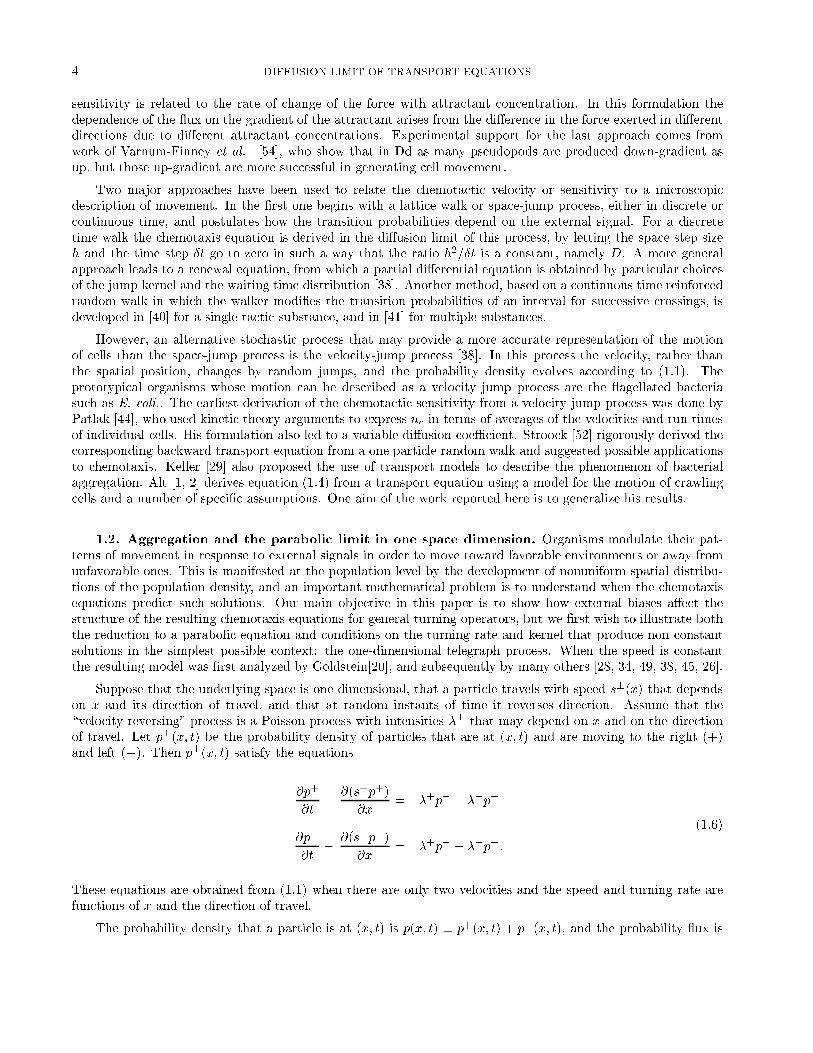
sensitivity is related to the rate of change of the force with attractant concentration. In this formulation thedependence of the ux on the gradient of the attractant arises from the di�erence in the force exerted in di�erentdirections due to di�erent attractant concentrations. Experimental support for the last approach comes fromwork of Varnum-Finney et al. [54], who show that in Dd as many pseudopods are produced down-gradient asup, but those up-gradient are more successful in generating cell movement.

Two major approaches have been used to relate the chemotactic velocity or sensitivity to a microscopicdescription of movement. In the �rst one begins with a lattice walk or space-jump process, either in discrete orcontinuous time, and postulates how the transition probabilities depend on the external signal. For a discretetime walk the chemotaxis equation is derived in the di�usion limit of this process, by letting the space step sizeh and the time step Æt go to zero in such a way that the ratio h2=Æt is a constant, namely D. A more generalapproach leads to a renewal equation, from which a partial di�erential equation is obtained by particular choicesof the jump kernel and the waiting time distribution [38]. Another method, based on a continuous time reinforcedrandom walk in which the walker modi�es the transition probabilities of an interval for successive crossings, isdeveloped in [40] for a single tactic substance, and in [41] for multiple substances.

However, an alternative stochastic process that may provide a more accurate representation of the motionof cells than the space-jump process is the velocity-jump process [38]. In this process the velocity, rather thanthe spatial position, changes by random jumps, and the probability density evolves according to (1.1). Theprototypical organisms whose motion can be described as a velocity jump process are the agellated bacteriasuch as E. coli.. The earliest derivation of the chemotactic sensitivity from a velocity jump process was done byPatlak [44], who used kinetic theory arguments to express uc in terms of averages of the velocities and run timesof individual cells. His formulation also led to a variable di�usion coeÆcient. Stroock [52] rigorously derived thecorresponding backward transport equation from a one particle random walk and suggested possible applicationsto chemotaxis. Keller [29] also proposed the use of transport models to describe the phenomenon of bacterialaggregation. Alt [1, 2] derives equation (1.4) from a transport equation using a model for the motion of crawlingcells and a number of speci�c assumptions. One aim of the work reported here is to generalize his results.

1.2. Aggregation and the parabolic limit in one space dimension. Organisms modulate their pat-terns of movement in response to external signals in order to move toward favorable environments or away fromunfavorable ones. This is manifested at the population level by the development of nonuniform spatial distribu-tions of the population density, and an important mathematical problem is to understand when the chemotaxisequations predict such solutions. Our main objective in this paper is to show how external biases a�ect thestructure of the resulting chemotaxis equations for general turning operators, but we �rst wish to illustrate boththe reduction to a parabolic equation and conditions on the turning rate and kernel that produce non constantsolutions in the simplest possible context: the one-dimensional telegraph process. When the speed is constantthe resulting model was �rst analyzed by Goldstein[20], and subsequently by many others [28, 34, 49, 38, 45, 26].

Suppose that the underlying space is one-dimensional, that a particle travels with speed s�(x) that dependson x and its direction of travel, and that at random instants of time it reverses direction. Assume that the\velocity-reversing" process is a Poisson process with intensities �� that may depend on x and on the directionof travel. Let p�(x; t) be the probability density of particles that are at (x; t) and are moving to the right (+)and left (�). Then p�(x; t) satisfy the equations

@p+

@t+@(s+p+)

@x= ��+p+ + ��p�

(1.6)@p�

@t� @(s�p�)

@x= �+p+ � ��p�:

These equations are obtained from (1.1) when there are only two velocities and the speed and turning rate arefunctions of x and the direction of travel.

The probability density that a particle is at (x; t) is p(x; t) � p+(x; t) + p�(x; t), and the probability ux is


j � (s+p+ � s�p�). These quantities satisfy the equations

@p

@t+

@j

@x= 0 (1.7)

@j

@t+ (�+ + ��)j = �s+ @

@x(s+p+)� s�

@

@x(s�p�) + (��s+ � �+s�)p (1.8)

and the initial conditions p(x; 0) = p0(x); j(x; 0) = j0(x), where p0 and j0 are determined from the initialdistribution of p+ and p�.

To illustrate how variable speeds and turning rates a�ect the existence of nonuniform steady states, whichcan be interpreted as aggregations, consider the system (1.7-1.8) on the interval (0,1) and impose homogeneousNeumann (no- ux) boundary conditions at both ends [39]. We �rst suppose that � is constant and determineunder what conditions, if any, these equations have time-independent, non-constant solutions for p�. Understeady state conditions the �rst equation implies that j is a constant, and the boundary conditions imply thatj � 0. Therefore s+p+ = s�p�, and the second equation reduces to

@

@x(s+p+) = �s+p+

�s+ � s�

s+s�

�: (1.9)

The solution of this equation is

p+(x) =s+(0)p+(0)

s+(x)e�

Z x

0

s+ � s�

s+s�d�� p+(0)F+(x);

and therefore the condition of vanishing ux gives p� as

p�(x) =s+(0)p+(0)

s�(x)e�

Z x

0

s+ � s�

s+s�d�� p+(0)F�(x):

It follows that p(x) � p+(x) + p�(x) is given by

p(x) = �

�1

s+(x)+

1

s�(x)

�e�

Z x

0

s+ � s�

s+s�d�; (1.10)

wherein � is a constant given by

� =Ns+(0)R 1

0(F+(�) + F�(�))d�

and N is the total number of cells in the unit interval. From this one can determine how the distribution of s�

a�ects the distribution of p. In particular, if s� are not constant then p� and p are also non-constant. This ismost easily seen if s+(x) = s�(x), for then it follows directly from (1.10) that cells accumulate at the minimaof the speed distribution. In any case, this simple model shows that cells can aggregate in a time-independentgradient by only modifying their speed, a process called orthokinesis. The case in which the velocities s� insystem (1.7) depend on the signal distribution S has been considered in [25], where the local and global existenceof solutions is established using the vanishing viscosity method.

It is also easy to see that particles cannot accumulate if the speed is symmetric and constant, but the turningrate � is symmetric and a function of x, i.e. if only local information is used to determine the rate of turning.When the speed is symmetric and constant but the turning rates are biased, the time-independent solution of(1.7-1.8) is given by j � 0 and

log p(x) = log p(0) +1

s

Z x

0

(�� +)d�;


where the constant log p(0) is determined by N . Clearly p(x) is identically p(0) when �� +. In the bacterialsystem described earlier the speed is essentially constant, but the turning rate depends on the history of exposureto the attractant or repellent, and hence on the path of the bacterium. In this case �� 6= �+ by virtue ofthe di�erent history of a particle moving up-gradient as compared with one moving down-gradient. By formallyignoring the time derivative of j in (1.8), or more precisely, considering the limit s; �!1; s2=2� � D = constant,the di�usion coeÆcient, one sees that in this case the chemotactic velocity is given by

uc = �s�+ � ��

2�� s�1

�:

The random and directed components of motion will be of the same order only if either �1 � O(p�) or �1 � O(s).

This case is studied in detail in [45, 26].

When both the speed and the turning rate are constant the system reduces to the telegraph equation

@2p

@t2+ 2�

@p

@t= s2

@2p

@x2(1.11)

and the di�usion equation results either by taking the limit �!1; s!1 with s2=2� � D constant as above, orby rescaling space and time appropriately, as in [23]. However, as we will show elsewhere, the stochastic telegraphprocess in higher space dimensions does not lead to the corresponding telegraph equation, even in the form of asystem similar to (1.7), and thus the conclusions reached for one space dimension may not carry over directly tohigher dimensions.

2. A brief summary of [23]. To make this paper self-contained we recall some results presented in [23]. Weconsider = IRn and we suppose that the velocities lie in a compact set V � IRn and that V is symmetric withrespect to the origin, which is no restriction for the applications to chemotaxis equations. In many applicationsit is assumed that the kernel T is symmetric or that it is continuous (see e.g. [1]). We can relax these conditionswith very little e�ort and still obtain a parabolic equation in the di�usion limit. Unless stated otherwise, weassume that � is constant.

Let K denote the cone of nonnegative functions in L2(V ), and for �xed (x; t) de�ne an integral operator Tand its adjoint T � by

T p =ZV

T (v; v0)p(x; v0; t)dv0; T � p =ZV

T (v0; v)p(x; v0; t)dv0: (2.1)

We impose the following conditions on the kernel and the integral operator.

(T1) T (v; v0) � 0;RVT (v; v0)dv = 1; and

RV

RVT 2(v; v0)dv0dv <1.

(T2) There are functions u0; �; and 2 K with u0 6� 0 and �; 6= 0 a.e. such that for all (v; v0) 2 V � V

u0(v)�(v0) � T (v0; v) � u0(v) (v

0): (2.2)

(T3) kT kh1i? < 1, where h1i? is the orthogonal complement in L2(V ) of the span of 1.(T4)

RVT (v; v0)dv0 = 1.

We de�ne the turning operator

Lp(v) = ��p(v) + �T p(v); (2.3)

acting in L2(V ), and then have the following conclusions concerning its spectral properties [23].

Theorem 2.1. Assume (T1)-(T4); then

1. 0 is a simple eigenvalue of L and the corresponding eigenfunction is �(v) � 1.


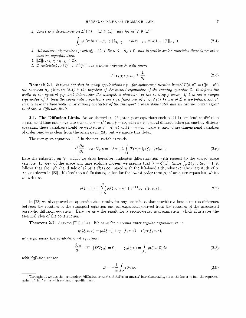
2. There is a decomposition L2(V ) = h1i � h1i? and for all 2 h1i?ZV

L dv � ��2k k2L2(V ); where �2 � �(1� kT kh1i?): (2.4)

3. All nonzero eigenvalues � satisfy �2� < Re � � ��2 < 0, and to within scalar multiples there is no otherpositive eigenfunction.

4. kLkL(L2(V );L2(V )) � 2�.

5. L restricted to h1i? � L2(V ) has a linear inverse F with norm

kFkL(h1i?;h1i?) �1

�2: (2.5)

Remark 2.1. It turns out that in many applications e.g., for symmetric turning kernel T (v; v0) = t(jv � v0j)the constant �2 given in (2.4) is the negative of the second eigenvalue of the turning operator L. It de�nes thewidth of the spectral gap and determines the dissipative character of the turning process. If 1 is not a simpleeigenvalue of T then the coordinate projections are eigenfunctions of T and the kernel of L is n+1-dimensional.In this case the hyperbolic or streaming character of the transport process dominates and we can no longer expectto obtain a di�usion limit.

2.1. The Di�usion Limit. As we showed in [23], transport equations such as (1.1) can lead to di�usionequations if time and space are scaled as � = �2t and � = �x, where � is a small dimensionless parameter. Strictlyspeaking, these variables should be written as � = �2 1t and � = � 2x, where 1 and 2 are dimensional variablesof order one, as is clear from the analysis in [23], but we ignore this detail.

The transport equation (1.1) in the new variables reads

�2@p

@�+ �v � r� p = ��p+ �

ZV

T (v; v0)p(�; v0; �)dv0; (2.6)

Here the subscript on r, which we drop hereafter, indicates di�erentiation with respect to the scaled spacevariable. In view of the space and time scalings chosen, we assume that � � O(1). Since

RVT (v; v0)dv = 1, it

follows that the right-hand side of (2:6) is O(1) compared with the left-hand side, whatever the magnitude of p.As was shown in [23], this leads to a di�usion equation for the lowest order term p0 of an outer expansion, whichwe write as

p(�; v; �) =

kXi=0

pi(�; v; �)�i + �k+1pk+1(�; v; �): (2.7)

In [23] we also proved an approximation result, for any order in �, that provides a bound on the di�erencebetween the solution of the transport equation and an expansion derived from the solution of the associatedparabolic di�usion equation. Here we give the result for a second-order approximation, which illustrates theessential idea of the construction.

Theorem 2.2. Assume (T1)-(T4). We consider a second order regular expansion in �:

q2(�; v; �) = p0(�; �) + �p1(�; v; �) + �2p2(�; v; �);

where p0 solves the parabolic limit equation

@p0@�

�r � �Drp0� = 0; p0(�; 0) =

ZV

p(�; v; 0)dv (2.8)

with di�usion tensor 1

D = � 1

!

ZV

vFvdv: (2.9)

1Throughout we use the terminology `di�usion tensor' and di�usion matrix' interchangeably, since the latter is just the represen-tation of the former with respect a speci�c basis.


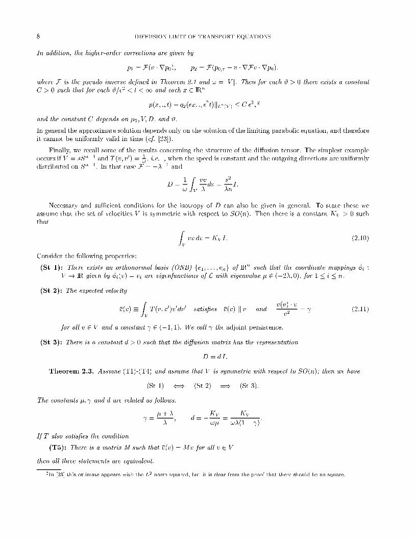
In addition, the higher-order corrections are given by

p1 = F(v � rp0); p2 = F(p0;� + v � rFv � rp0);

where F is the pseudo inverse de�ned in Theorem 2.1 and ! = jV j. Then for each # > 0 there exists a constantC > 0 such that for each #=�2 < t <1 and each x 2 IRn

kp(x; :; t)� q2(�x; :; �2t)kL2(V ) � C �3; 2

and the constant C depends on �2; V;D; and #.

In general the approximate solution depends only on the solution of the limiting parabolic equation, and thereforeit cannot be uniformly valid in time (cf. [23]).

Finally, we recall some of the results concerning the structure of the di�usion tensor. The simplest exampleoccurs if V = sSn�1 and T (v; v0) = 1

!, i.e. , when the speed is constant and the outgoing directions are uniformly

distributed on Sn�1. In that case F = ��1 and

D =1

!

ZV

vv

�dv =

s2

�nI:

Necessary and suÆcient conditions for the isotropy of D can also be given in general. To state these weassume that the set of velocities V is symmetric with respect to SO(n). Then there is a constant KV > 0 suchthat Z

V

vv dv = KV I: (2.10)

Consider the following properties:

(St 1): There exists an orthonormal basis (ONB) fe1; : : : ; eng of IRn such that the coordinate mappings �i :V ! IR given by �i(v) = vi are eigenfunctions of L with eigenvalue � 2 (�2�; 0), for 1 � i � n.

(St 2): The expected velocity

�v(v) �ZV

T (v; v0)v0dv0 satis�es �v(v) k v and�v(v) � vv2

= (2.11)

for all v 2 V and a constant 2 (�1; 1): We call the adjoint persistence.

(St 3): There is a constant d > 0 such that the di�usion matrix has the representation

D = d I:

Theorem 2.3. Assume (T1)-(T4) and assume that V is symmetric with respect to SO(n); then we have

(St 1) () (St 2) =) (St 3):

The constants �; and d are related as follows.

=�+ �

�; d = �KV

!�=

KV

!�(1� ):

If T also satis�es the condition

(T5): There is a matrix M such that �v(v) =Mv for all v 2 Vthen all three statements are equivalent.

2In [23] this estimate appears with the L2-norm squared, but it is clear from the proof that there should be no square.


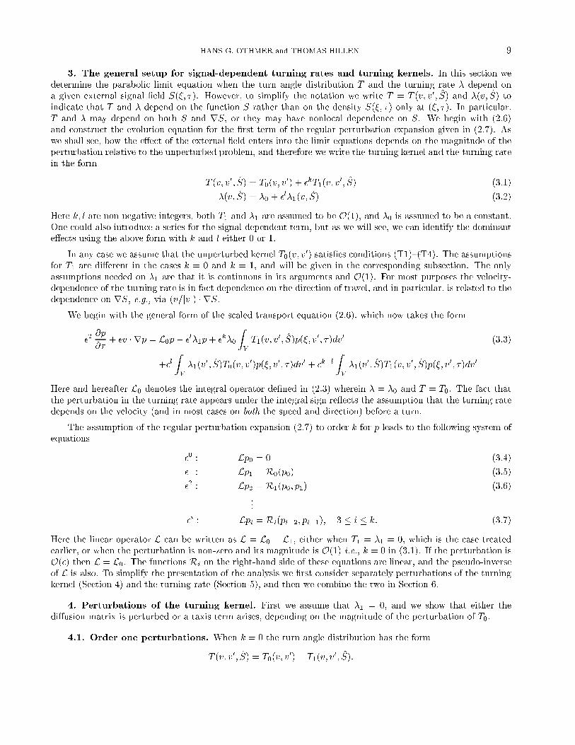
3. The general setup for signal-dependent turning rates and turning kernels. In this section wedetermine the parabolic limit equation when the turn angle distribution T and the turning rate � depend ona given external signal �eld S(�; �). However, to simplify the notation we write T = T (v; v0; S) and �(v; S) toindicate that T and � depend on the function S rather than on the density S(�; �) only at (�; �). In particular,T and � may depend on both S and rS, or they may have nonlocal dependence on S. We begin with (2.6)and construct the evolution equation for the �rst term of the regular perturbation expansion given in (2.7). Aswe shall see, how the e�ect of the external �eld enters into the limit equations depends on the magnitude of theperturbation relative to the unperturbed problem, and therefore we write the turning kernel and the turning ratein the form

T (v; v0; S) = T0(v; v0) + �kT1(v; v

0; S) (3.1)

�(v; S) = �0 + �l�1(v; S) (3.2)

Here k; l are non-negative integers, both T1 and �1 are assumed to be O(1), and �0 is assumed to be a constant.One could also introduce a series for the signal-dependent term, but as we will see, we can identify the dominante�ects using the above form with k and l either 0 or 1.

In any case we assume that the unperturbed kernel T0(v; v0) satis�es conditions (T1){(T4). The assumptions

for T1 are di�erent in the cases k = 0 and k = 1, and will be given in the corresponding subsection. The onlyassumptions needed on �1 are that it is continuous in its arguments and O(1). For most purposes the velocity-dependence of the turning rate is in fact dependence on the direction of travel, and in particular, is related to thedependence on rS, e.g., via (v=jvj) � rS.

We begin with the general form of the scaled transport equation (2.6), which now takes the form

�2@p

@�+ �v � rp = L0p� �l�1p+ �k�0

ZV

T1(v; v0; S)p(�; v0; �)dv0 (3.3)

+�lZV

�1(v0; S)T0(v; v

0)p(�; v0; �)dv0 + �k+lZV

�1(v0; S)T1(v; v

0; S)p(�; v0; �)dv0

Here and hereafter L0 denotes the integral operator de�ned in (2.3) wherein � = �0 and T = T0. The fact thatthe perturbation in the turning rate appears under the integral sign re ects the assumption that the turning ratedepends on the velocity (and in most cases on both the speed and direction) before a turn.

The assumption of the regular perturbation expansion (2.7) to order k for p leads to the following system ofequations

�0 : Lp0 = 0 (3.4)

�1 : Lp1 = R0(p0) (3.5)

�2 : Lp2 = R1(p0; p1) (3.6)

...

�i : Lpi = Ri(pi�2; pi�1); 3 � i � k: (3.7)

Here the linear operator L can be written as L = L0 + L1, either when T1 = �1 = 0, which is the case treatedearlier, or when the perturbation is non-zero and its magnitude is O(1) i.e., k = 0 in (3.1). If the perturbation isO(�) then L = L0. The functions Ri on the right-hand side of these equations are linear, and the pseudo-inverseof L is also. To simplify the presentation of the analysis we �rst consider separately perturbations of the turningkernel (Section 4) and the turning rate (Section 5), and then we combine the two in Section 6.

4. Perturbations of the turning kernel. First we assume that �1 = 0, and we show that either thedi�usion matrix is perturbed or a taxis term arises, depending on the magnitude of the perturbation of T0.

4.1. Order one perturbations. When k = 0 the turn angle distribution has the form

T (v; v0; S) = T0(v; v0) + T1(v; v

0; S):


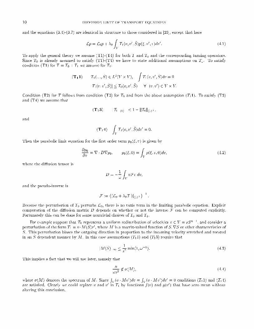
and the equations (3.4)-(3.7) are identical in structure to those considered in [23], except that here

Lp = L0p+ �0

ZV

T1(v; v0; S)p(�; v0; �)dv0: (4.1)

To apply the general theory we assume (T1)-(T4) for both T and T0 and the corresponding turning operators.Since T0 is already assumed to satisfy (T1)-(T4) we have to state additional assumptions on T1. To satisfycondition (T1) for T = T0 + T1 we assume for T1:

(T11) T1(:; :; S) 2 L2(V � V );

ZT1(v; v

0; S)dv = 0

jT1(v; v0; S)j � T0(v; v0; S) 8 (v; v0) 2 V � V:

Condition (T2) for T follows from condition (T2) for T0 and from the above assumption (T11). To satisfy (T3)and (T4) we assume that

(T13) kT1kh1i? < 1� kT0kh1i? ;

and

(T14)

ZV

T1(v; v0; S)dv0 = 0:

Then the parabolic limit equation for the �rst order term p0(�; �) is given by

@p0@�

= r �Drp0; p0(�; 0) =

ZV

p(�; v; 0)dv; (4.2)

where the di�usion tensor is

D = � 1

!

ZV

vFv dv;

and the pseudo-inverse is

F :=�(L0 + �0T1)jh1i?

��1:

Because the perturbation of T0 perturbs L0, there is no taxis term in the limiting parabolic equation. Explicitcomputation of the di�usion matrix D depends on whether or not the inverse F can be computed explicitly.Fortunately this can be done for some nontrivial choices of T0 and T1.

For example suppose that T0 represents a uniform redistribution of velocities v 2 V = sSn�1, and consider aperturbation of the form T1 = v �M(S)v0, whereM is a matrix-valued function of S;rS or other characteristics ofS. This perturbation biases the outgoing direction in proportion to the incoming velocity stretched and rotatedin an S-dependent manner by M . In this case assumptions (T11) and (T13) require that

kM(S)k1 � 1

s2min(1; !�1): (4.3)

This implies a fact that we will use later, namely that

n

!s262 �(M); (4.4)

where �(M) denotes the spectrum of M . SinceRV(v �Mv0)dv =

RV(v �Mv0)dv0 = 0 conditions (T11) and (T14)

are satis�ed. Clearly we could replace v and v0 in T1 by functions f(v) and g(v0) that have zero mean withoutaltering this conclusion.


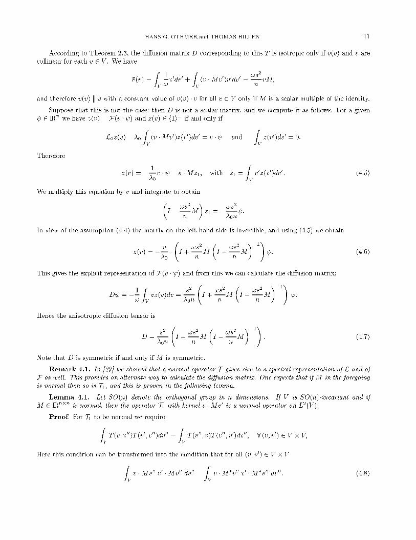
According to Theorem 2.3, the di�usion matrix D corresponding to this T is isotropic only if �v(v) and v arecollinear for each v 2 V . We have

�v(v) =

ZV

1

!v0dv0 +

ZV

(v �Mv0)v0dv0 =!s2

nvM;

and therefore �v(v) k v with a constant value of �v(v) � v for all v 2 V only if M is a scalar multiple of the identity.

Suppose that this is not the case; then D is not a scalar matrix, and we compute it as follows. For a given 2 IRn we have z(v) = F(v � ) and z(v) 2 h1i? if and only if

L0z(v) + �0

ZV

(v �Mv0)z(v0)dv0 = v � and

ZV

z(v0)dv0 = 0:

Therefore

z(v) = � 1

�0v � + v �Mz1; with z1 =

ZV

v0z(v0)dv0: (4.5)

We multiply this equation by v and integrate to obtain�I � !s2

nM

�z1 = �!s

2

�0n :

In view of the assumption (4.4) the matrix on the left hand side is invertible, and using (4.5) we obtain

z(v) = � v

�0� I +

!s2

nM

�I � !s2

nM

��1! : (4.6)

This gives the explicit representation of F(v � ) and from this we can calculate the di�usion matrix:

D = � 1

!

ZV

vz(v)dv =s2

�0n

I +

!s2

nM

�I � !s2

nM

��1! :

Hence the anisotropic di�usion tensor is

D =s2

�0n

I +

!s2

nM

�I � !s2

nM

��1!: (4.7)

Note that D is symmetric if and only if M is symmetric.

Remark 4.1. In [23] we showed that a normal operator T gives rise to a spectral representation of L and ofF as well. This provides an alternate way to calculate the di�usion matrix. One expects that if M in the foregoingis normal then so is T1, and this is proven in the following lemma.

Lemma 4.1. Let SO(n) denote the orthogonal group in n dimensions. If V is SO(n)-invariant and ifM 2 IRn�n is normal, then the operator T1 with kernel v �Mv0 is a normal operator on L2(V ).

Proof. For T1 to be normal we requireZV

T (v; v00)T (v0; v00)dv00 =

ZV

T (v00; v)T (v00; v0)dv00; 8 (v; v0) 2 V � V;

Here this condition can be transformed into the condition that for all (v; v0) 2 V � VZV

v �Mv00 v0 �Mv00 dv00 =

ZV

v �M�v00 v0 �M�v00 dv00: (4.8)


Since M is assumed to be normal and M has real entries there is an 2 SO(n) such that M� = M. We usethis in (4.8) and substitute w = v00. Then the right hand side of (4.8) equalsZ

V

v �Mw v0 �Mw det(�1) dw:

Since is orthogonal, its determinant is �1. For +1 (4.8) is valid, and for �1 we substitute y = �w and againobserve that (4.8) indeed is true.

In particular, we consider a system of individuals which show a certain direction of anisotropy b 2 IRn. Thisapplies, for example, to a stream of elongated bacteria such as myxobacteria that is oriented in the direction b.The following turning kernel describes a tendency toward alignment in the the direction of the stream.

T1 = �(v � b)(v0 � b); jbj = 1:

If the actual direction v0 is in the direction b or �b, then there is an increased probability to choose a new velocityv in the direction b or �b, respectively. When moving in the direction of the stream this kernel re ects a tendencyto move forward or backward of magnitude � �s2. In the notation used above we have M = �bb and condition(4.3) reads in this case

� � 1

s2min (1; !�1):

The corresponding di�usion matrix is

D(�; �) =s2

�0n

I +

!s2

n�bb

�I � !s2

n�bb

��1!;

The di�usivity in the direction b or �b is enhanced, whereas it has the value s2=�0n in the orthogonal direction,as in the unbiased case.

Remark 4.2. We can summarize the results for an order one perturbation of T0 as follows. Due to the factthat the organisms sense and respond to the external �eld, we obtain an anisotropic di�usion tensor D. However,there is no taxis component in the di�usion approximation, and as we observed earlier, because the evolutionequation for p0 has the form (4.2), there are no nonconstant steady state solutions under Neumann boundaryconditions in this case. Thus, if the e�ect of the external �eld is of the same order as the reorientation in theabsence of the external �eld, there is no taxis and no steady-state aggregation. The secondary restrictions on themagnitude of the perturbation, as re ected in (4.3), are essential. Without these a suÆciently large perturbationwould destroy the ellipticity of the space operator in the limiting equation, and the di�usion limit would not bevalid. It is not known what the appropriate form of the limiting equation is when (4.3) is not satis�ed. Onepossibility is that the evolution from general initial data never relaxes to the parabolic regime. This could occur,for example, if the convection in v-space is on the same or a faster time scale than relaxation of the velocitychanges. In those cases the turning operator loses its dissipative character.

As we will see in the following section, a weaker perturbation leads to a taxis component in the evolutionequation for p0.

4.2. O(�) perturbations. Next we consider O(�) perturbations to T0, i.e., k = 1 in (3.1). In this caseL = L0 and the only assumptions on T1 are that this perturbation gives rise to a well de�ned Cauchy problemand that the total particle mass is preserved. To satisfy (T1) for the perturbed kernel we assume that for each S

(T110) T1(:; :; S) 2 L2(V � V ) and

ZT1(v; v

0; S)dv = 0:

We �rst derive the general form of the chemotactic velocity in terms of properties of the bias T1 of the turningoperator, without a detailed speci�cation as to how T1 depends on the external signal, and thereby show how toderive the chemotaxis equation (1.2) from the microscopic model of the motion. We then examine several forms


for the dependence of the kernel on S and its gradient, some of which lead to the classical PKSA equation, andothers which lead to more general equations.

For an O(�) perturbation it follows as in [23] that p0 = p0(�; �). The O(�) equation now reads

L0p1 = (v � r � �0�1(v))p0; (4.9)

where the directional distributions �i, are de�ned as

�i(v) =

ZV

Ti(v; v0)dv0 (4.10)

for i = 0; 1. The distribution �0 gives the total probability of an outgoing direction v for all incoming velocitiesv0, whereas the O(�) shift in the outgoing velocity distribution is given by the directional bias �1. The averagedirectional bias is Z

V

�1(v)dv = 0

by virtue of condition (T110) and Fubini's theorem. The solvability condition is satis�ed, becauseZ

(v � rp0)dv = 0;

and therefore p1 is given by

p1 = F0(v � rp0)� �0F0(�1(v)p0):

Here F0 denotes the pseudo inverse of L0.The evolution equation for p2 reads

�2 : L0p2 = @p0@�

+ v � rp1 � �0

ZV

T1(v; v0; S)p1(v

0)dv0:

The solvability condition is

0 =

ZV

�@p0@�

+ (v � r)F0(v � rp0)� �0(v � r)F0(�1(v)p0�dv

� �0

ZV

ZV

T1(v; v0; S)p1(v

0)dv0dv:

and the last term vanishes because of assumption (T110). If we de�ne the chemotactic velocity as

uc � ��0!

ZV

vF0�1(v)dv = ��0!

ZV

ZV

vF0T1(v; v0; S)dv0dv; (4.11)

then the solvability condition leads to an equation equivalent to (1.2), namely

@p0@�

= r � (Drp0 � ucp0) ; (4.12)

where as before D = �!�1 RVvF0vdv and uc depends on S. The macroscopic chemotactic velocity de�ned by

(4.11) is simply the �rst moment of the directional bias distribution transformed by the pseudo inverse F0, andas such, represents an average velocity formed by weighting the microscopic velocities by the transform of thedirectional bias. Note that if we were to impose condition (T14) on T1, the chemotactic velocity would vanish.Thus the `reversibility' imposed on the unbiased turning operator precludes chemotaxis if imposed on the O(�)bias of the turning operator.


4.2.1. T1 linear in rS: The PKSA equation. Thus far a general dependence on S in the kernel T1is admissible, but to obtain the classical chemotaxis equation we must specify both T0 and how T1 depends onthe external signal. As we have seen before, the case T0 = 1=! and V = sSn�1 is simplest, since we know F0explicitly, and in this case the di�usion matrix and the chemotactic velocity are given by

D =s2

�0nI

uc =1

!

ZV

v�1(v)dv =1

!

ZV

vT1(v; v0; S)dv0dv:

Since the pseudo inverse is simply multiplication by ��10 for this choice of T0, the macroscopic chemotacticvelocity de�ned by (4.11) is proportional to the �rst moment of the directional bias distribution. A necessarycondition to obtain the PKSA equation is that T1 depends linearly on rS, in the form T1 = Q1(v; v

0; S) � rS,where Q1(v; v

0; S) is a vector valued function of v; v0 and S that satis�esZV

Q1(v; v0; S)dv = 0: (4.13)

In this case the directional bias (4.10) is given by

�1(v) =

ZV

Q1(v; v0; S)dv0 � rS � q1(v; S) � rS: (4.14)

The vector q1(v; S) is the average velocity in the direction of v, taken over a uniform distribution of incomingvelocities. The chemotactic velocity can now be written as the linear transformation of rS given by

uc(S;rS) = �(S)rS; (4.15)

where the chemotactic sensitivity is given by the matrix

�(S) � 1

!

ZV

ZV

vQ1(v; v0; S)dv0dv =

1

!

ZV

vq1(v; S)dv: (4.16)

It is clear that this may or may not reduce to a scalar sensitivity, even though the di�usion process generated byT0 is isotropic.

In particular, suppose that Q1 has the form

Q1(v; v0; S) = k1(v

0; S)v (4.17)

for a positive scalar function k1 in the foregoing analysis. Then whenever v is in the direction of rS (i.e.rS �v > 0)the term T1 increases the probability of choosing v as the new direction compared to T0 alone. If v and rS areopposite this probability is reduced compared with that for no bias. Here q1 = (

RVk1(v

0; S)dv0)v � k(S)v, andthe chemotactic sensitivity matrix reduces to the scalar chemotactic sensitivity

�(S) = k(S)s2

!n=�0k(S)

!D:

The parabolic limit equation now reads

@p0@�

= r � (Drp0 � p0�(S)rS) ; (4.18)

which is of the PKSA form. Any other combination of kernels T0 that generate isotropic di�usion and perturba-tions of the form k(S)v � rS will also lead to the PKSA equation. In particular, the kernel T0 may incorporatepersistence.

The same analysis can be carried through for a general kernel T0, the only change being that the chemotacticsensitivity now becomes

�(S) � ��0!

ZV

vF0q1(v; S)dv: (4.19)


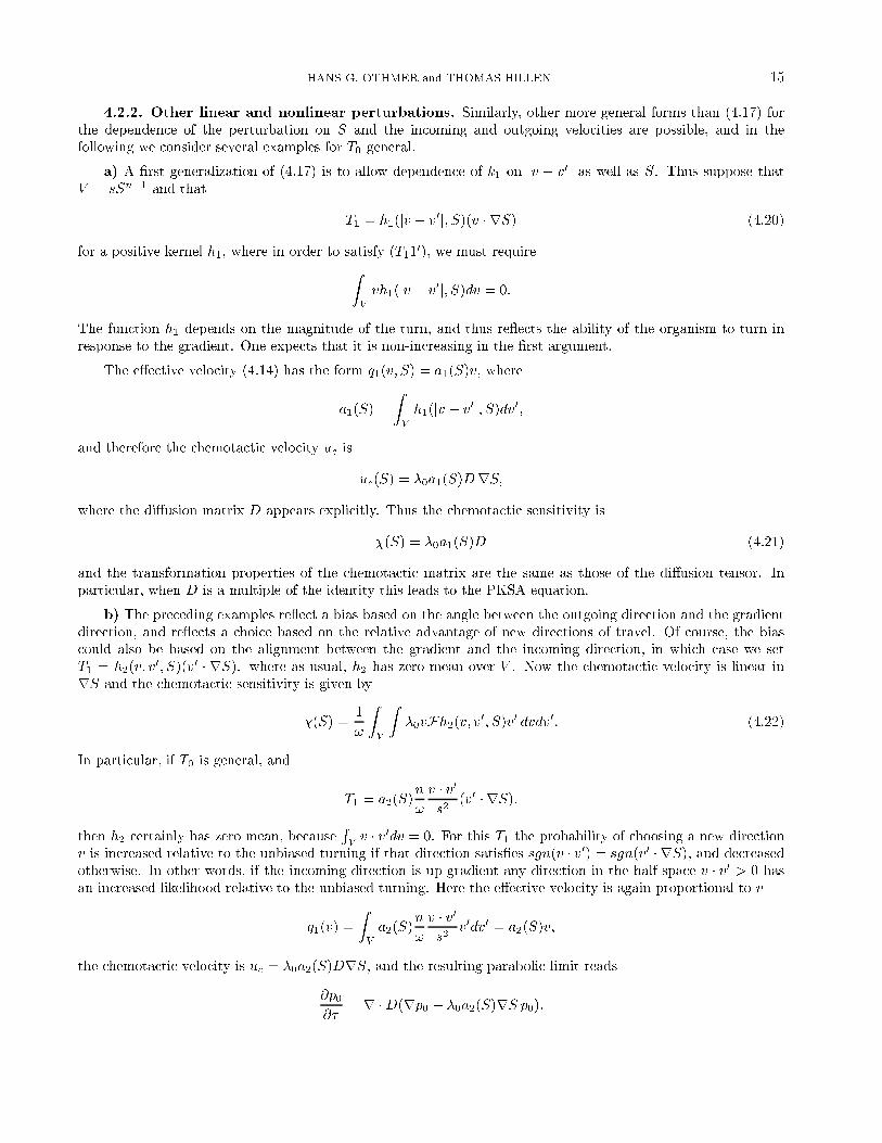
4.2.2. Other linear and nonlinear perturbations. Similarly, other more general forms than (4.17) forthe dependence of the perturbation on S and the incoming and outgoing velocities are possible, and in thefollowing we consider several examples for T0 general.

a) A �rst generalization of (4.17) is to allow dependence of k1 on jv � v0j as well as S. Thus suppose thatV = sSn�1 and that

T1 = h1(jv � v0j; S)(v � rS) (4.20)

for a positive kernel h1, where in order to satisfy (T110), we must requireZ

V

vh1(jv � v0j; S)dv = 0:

The function h1 depends on the magnitude of the turn, and thus re ects the ability of the organism to turn inresponse to the gradient. One expects that it is non-increasing in the �rst argument.

The e�ective velocity (4.14) has the form q1(v; S) = a1(S)v, where

a1(S) =

ZV

h1(jv � v0j; S)dv0;

and therefore the chemotactic velocity uc is

uc(S) = �0a1(S)DrS;

where the di�usion matrix D appears explicitly. Thus the chemotactic sensitivity is

�(S) = �0a1(S)D (4.21)

and the transformation properties of the chemotactic matrix are the same as those of the di�usion tensor. Inparticular, when D is a multiple of the identity this leads to the PKSA equation.

b) The preceding examples re ect a bias based on the angle between the outgoing direction and the gradientdirection, and re ects a choice based on the relative advantage of new directions of travel. Of course, the biascould also be based on the alignment between the gradient and the incoming direction, in which case we setT1 = h2(v; v

0; S)(v0 � rS). where as usual, h2 has zero mean over V . Now the chemotactic velocity is linear inrS and the chemotactic sensitivity is given by

�(S) =1

!

ZV

Z�0vFh2(v; v0; S)v0 dvdv0: (4.22)

In particular, if T0 is general, and

T1 = a2(S)n

!

v � v0s2

(v0 � rS):

then h2 certainly has zero mean, becauseRVv � v0dv = 0. For this T1 the probability of choosing a new direction

v is increased relative to the unbiased turning if that direction satis�es sgn(v � v0) = sgn(v0 � rS), and decreasedotherwise. In other words, if the incoming direction is up-gradient any direction in the half-space v � v0 > 0 hasan increased likelihood relative to the unbiased turning. Here the e�ective velocity is again proportional to v

q1(v) =

ZV

a2(S)n

!

v � v0s2

v0dv0 = a2(S)v;

the chemotactic velocity is uc = �0a2(S)DrS, and the resulting parabolic limit reads

@p0@�

= r �D(rp0 � �0a2(S)rS p0):


Again, for scalar D this is the PKSA equation.

c) In the foregoing the perturbations are all linear in the gradient of the external signal, but there is no apriori reason to restrict attention to this case. The �nal example shows how nonlinear dependence on the gradientcan arise very naturally.

Let T0 be a general kernel and suppose that T1 depends on the angle

� = arccos

�v � rSjvjjrSj

�:

In this case it is more appropriate to consider an expansion in Legendre polynomials Pj(cos�), rather thanassuming a Fourier expansion of T1 in �. We assume for some J 2 IN; J > 0 that

T1(v; v0; S) =

JXj=0

aj(S)Pj(cos�):

The chemotactic velocity is given by

uc = ��0!

ZV

ZV

vF0JX

j=0

aj(S)Pj

�v � rSjvjjrSj

�dvdv0;

which is clearly nonlinear in rS. In the particular case V = sSn�1; T0 = 1=!, the pseudo inverse F0 is multipli-cation with ��10 . Since the V domain is symmetric, all integrals involving odd powers of v vanish, and it followsthat uc is a polynomial in rS of highest order J (resp., J � 1 ) for J odd (resp., even).

5. Perturbations of the turning rate. In this section we analyze the e�ect of perturbations in the turningrate for a �xed turning kernel T0. We �rst consider an additive bias, and then show how the theoretical resultsapply to bacterial chemotaxis. We only consider the case of an O(�) additive perturbation, since an order oneadditive perturbation in the turning rate leads to an operator L whose spectral properties cannot be determinedin general. In the case of an O(�) perturbation we have L = L0, and we �nd that R0 in (3.5) is given by

R0(p0) = v � rp0 + �1(v; S)p0 �ZV

�1(v0; S)T0(v; v

0)p0(�; v0; �)dv0: (5.1)

Therefore p1 = F0(R0(p0)), and the O(�2) equation becomes

L0p2 = @p0@�

+R0(F(R0(p0))): (5.2)

The solvability condition readsZV

�@p0@�

+

�v � r+ �1(v; S)�

ZV

�1(v0; S)T0(v; v

0)(�)dv0��

(5.3)

F0�v � r+ �1(v; S)� ��1(v; S)

�p0(�; �)

idv = 0

where

��1(v; S) =

ZV

�1(v0; S)T0(v; v

0)dv0 (5.4)

is the average bias, over all incoming velocities, of the rate of turning to v. ClearlyR(�1 � ��1)dv vanishes when

�1 is independent of the velocity.


The solvability condition (5.3) can be written

0 =

ZV

@p0@�

dv +

�r �ZV

vF0vdvr�p0 +r �

�ZV

vF0(�1 � ��1)dv

�p0

+

� ZV

�1(v; S)F0�v � r+ �1(v; S)� ��1(v; S)

�dv

�ZV

Z�1(v

0; S)T0(v; v0)F0

�v0 � r+ �1(v

0; S)� ��1(v0; S)

�dv0dv

�p0;

and it follows from condition (T1) for T0 that the operator in square brackets is identically zero. Therefore thefollowing parabolic limit equation remains

@p0@�

= r � (Drp0 � ucp0): (5.5)

As before the di�usion tensor is given by

D = � 1

!

ZV

vF0v dv

and the chemotactic velocity is now given by

uc = � 1

!

ZV

vF0(�1(v; S)� ��1(v; S))dv:

For example, if V = sSn�1 and T0 = !�1 the linear functional F0 is multiplication by ��10 . Hence

D = s2=(�0n) and ��1(S) = 1=!RV�1(v

0; S)dv0 does not depend on v 2 V . Then the chemotactic velocity is

uc(S) =1

�0!

ZV

v�1(v; S)dv;

which is proportional to the �rst moment of �1 with respect to v.

As a second example, suppose that

�1(v; S) = �(v; S) � rS;whereupon

uc(S) = �(S) � rS;with �rst moment

�(S) =1

�0!

ZV

v�(v; S)dv: (5.8)

Hence again we obtain the classical (PKSA) chemotaxis equation

@p0@�

= r ��s2

�0nrp0 � p0�(S)rS

�:

5.1. Application to bacterial chemotaxis. Ford and co-workers [17, 16] have studied bacterial chemotaxisusing a stopped ow di�usion chamber (SFDC). In [17, 10] they use mathematical models based on transportequations and their di�usion limit to model the experiments and to identify the relevant parameters. The analysisis based on earlier work by Rivero et al. [45], in which taxis is described in one space dimension using experimental�ts to the turning rate developed in [7]. Here we show that the general formulation developed above can be useddirectly in any number of space dimensions.


Berg and Brown [4] and Macnab [33] observed experimentally that the turning kernel for E. coli andSalmonella typhimurium only depends on the relative angle � between the old and the new direction, whereas usual

� = arccos

�v � v0jvjjv0j

�:

Their results can be �t using

T (v; v0) =f(�)

2� sin �:

where f is a sixth-order polynomial that is nonnegative and satis�es f(0) = f(�) = 0 (cf eqn(40) of [10]), andnormalized so that Z

V

T (v; v0)dv0 =

ZV

T (v; v0)dv = 1:

The mean turning angle that emerges from the data is approximately 68 degrees, rather than the 90 degreesexpected if the distribution of new directions is uniform on S2.

Since T depends only on the angle �, we can apply the conclusions in Remark 3.4 of [23]. In the notation usedthere we have T (v; v0) = h(�) with h = f=(2� sin). Since this kernel is symmetric the di�usion limit automaticallyis isotropic. The di�usion constant is given by

d :=s2

n�0(1� d)(5.9)

where the persistence d is

d = 2�

Z �

0

h(�) cos � sin �d� =

Z �

0

f(�) cos �d� (5.10)

(cf. [38] or eqn (3.26) in [23]). For n = 1 the above representation of the di�usion constant corresponds to eqn(17)in [16], where a one dimensional chemotaxis model was studied. Note that this representation breaks down whenthe persistence is large, and other scalings have to be introduced.

In the presence of a gradient of an extracellular signal S(x; t), Block et al. [7] found that the experimentalobservations on tumbling in E. coli can be �t by assuming that tumbles are generated by a Poisson process whoseintensity depends on the rate of change of the fraction

f =S

KD + S

of occupied receptors. Here KD is the dissociation constant for the attractant. For a swimming bacterium thisleads to the expression

�(x; v; t; S) = �0 exp

�� c1KD

(KD + S)2(St + v � rS)

�; (5.11)

where �0 is the turning rate in the absence of the chemical signal and c1 is the change in the turning rate perunit of change in df=dt. A similar relation was �rst derived by Nossal [36]. Rivero et al. [45] and Ford et al. [17]use this in one space dimension and derive expressions for the di�usion constant and the chemotactic sensitivity.

In the parabolic scaling used above (� = �2t; � = �x) we can expand this as a function of �, and to �rst orderwe have

�(�; v; �; S) = �0 exp

�� c1KD

(KD + S)2��2St + �v � rS�� ;

= �0

�1� �

c1KD

(KD + S)2(v � rS) +O(�2)

�:


Therefore the chemotactic velocity is given by

uc = �(S)rSand the chemotactic sensitivity is

�(S) = c1s2

n

KD

(KD + S)2; (5.12)

which corresponds to formula (15) in [16] when n = 1. Note that to lowest order in � the local rate of changedoes not a�ect the chemotactic velocity; only the spatial gradient enters. This is of course based on the implicitassumption that the temporal derivatives are O(1) on the t scale.

Thus earlier results derived for one dimension can easily be extended to two or three dimensions and lead tothe equation

@p0@�

= r � (drp0 � p0�(S)rS);with

d =s2

n�0(1� d)and �(S) =

c1s2

n

KD

(KD + S)2:

The proportionality factors connecting 3D cell speed to one dimensional projections and other relations concerningthe dimensionality of the equations are discussed in [11] and [23].

It should be noted that the chemotactic sensitivity does not involve the directional persistence, and that itvanishes when c1 = 0, i.e. , when the turning rate does not depend on the change in occupancy of the receptors.In that case the taxis vanishes and there can be no aggregation. Said otherwise, this formulation is consistentwith the experimental observation that no adaptation implies no aggregation [55]. A di�erent phenomenologicalapproach that incorporates adaptation is analyzed in [50].

6. Combination of the perturbations � = �0 + ��1 and T = T0 + �T1. As we remarked in theintroduction, the slime mold Dd uses both taxis and kinesis, in that they move slightly faster when traveling upthe gradient, they correct the direction of travel to approach the gradient direction, and they decrease the turningrate. The �rst e�ect is small, and thus this system is an example of combined run length control and taxis.

When perturbations of both the turning rate and the turning kernel are admitted the scaled transport equation(3.3) has the form

�2@p

@�+ �(v � r)p = L0p+ �

��1p�

ZV

�1(v0; S)T0(v; v

0)p(v0; x; t)dv0�

��0ZV

T1(v; v0; S)p(v0; x; t)dv0 +O(�2):

The perturbations enter additively at order �, and the order �2 term does not change the limiting equation. Hencewe obtain

@p0@�

= r � (Drp0 � ucp0);

where

D = � 1

!

ZV

vF0v dv;

uc = ��0!

ZV

vF0�1(v)dv � 1

!

ZV

vF0(�1(v; S)� ��1(v; S)dv:

Here

�1(v) =

ZV

T1(v; v0; S)dv0 and ��1(v) =

ZV

�1(v0; S)T0(v; v

0)dv0:


7. Inclusion of nonlocal sensing and birth-death processes.

7.1. Nonlocal dependence on the signal distribution. A long-standing question in chemotaxis is howsmall organisms such as bacteria or amoeboid cells extract directional information from a scalar extracellular �eldsuch as the concentration of an attractant. In the case of bacteria it is clear that the body length is too short tomeasure gradients along the body axis, whereas amoeba may be able to e�ectively measure and compare di�erentconcentrations on di�erent sites on their cell surface. Related to this issue is the question of what the e�ectivesampling volume is in which the signal is signi�cant. This volume depends on how rapidly a receptor processesthe signal [5]. For E. coli the o� rate for the Tar receptor is 70 sec�1 [51], and thus the sampling volume is small,while in Dd the o� rate is � 0:45 sec�1, and the e�ective sampling volume is many times the cell volume [39].

A simple mathematical model that may capture the essence of both an e�ective sampling volume and amechanism for extracting directional information is as follows. For simplicity we assume that a cell can beapproximated as a sphere, and we denote its center by x and the e�ective sampling radius by R. Consider thequantity

ÆS (x; t) =

n

!0R

ZSn�1

� S(x+R�; t) d�; (7.1)

where � is the unit outer normal and !0 is the area of the unit (n-1)-sphere. The integral represents the dominantdirection in the extracellular signal at a distance R from the center, which could be the cell radius, and hence ifcells can `compute' this integral they can extract directional information from a scalar extracellular �eld without

measuring a gradient. Note thatÆ

S vanishes if S is spatially uniform, as it should. A simple mechanism by which

cells could computeÆ

S is to produce an intracellular signal in proportion to the number of receptors occupied andcondition the response on the local level of this substance. A molecular mechanism based on a local activatorand a long-range inhibitor or adaptation e�ector is currently under investigation [8].

As the sensing radius R ! 0 this expression approximates the local gradient of S, which can be seen asfollows (we suppress the time dependence in the following calculation):

ÆS (x) =

n

!0R

ZV

�

�S(x) +R(� � r)S(x) + R2

2(� � r)(� � r)S(x) + h.o.t.

�d� (7.2)

=n

!0R

�ZV

�d�S(x) +R

ZV

��d�rS(x) +O(R2)

�= rS(x) +O(R):

To derive chemotaxis equations we treat the non local `gradient'Æ

S in exactly the same way as we used rSin the previous sections. In particular for order �-perturbations of the form

h1(jv � v0j)(v� ÆS);which is analogous to (4.20), we obtain the chemotaxis equation

@p0@�

= r � (Drp0 � �(S)p0Æ

S) (7.3)

with �(S) given by (4.21). This, combined with the signal equation (1.5), leads to an integro-di�erential model

for chemotaxis. In addition, perturbations of the turning rate are given by replacing rS byÆ

S in section 5. Inparticular

� = �0 + �� ÆSleads to (7.3) with �(S) given by (5.8).

In some cases an integro-di�erential equation for the species density such as (7.3) may be replaced by afourth-order partial di�erential equation [37]. In the expansion (7.2), the R2-term vanishes because it is odd in�. Therefore the next correction to the gradient is the third derivative of S, which gives a fourth-order term in(7.3).


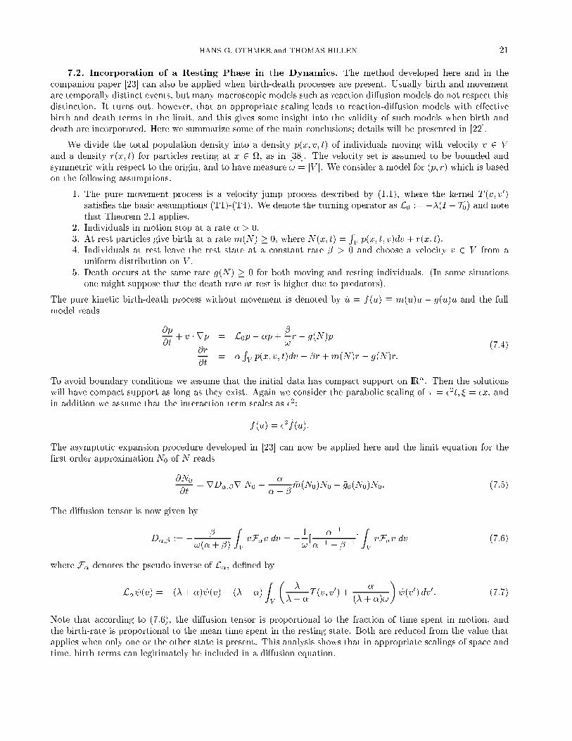
7.2. Incorporation of a Resting Phase in the Dynamics. The method developed here and in thecompanion paper [23] can also be applied when birth-death processes are present. Usually birth and movementare temporally distinct events, but many macroscopic models such as reaction di�usion models do not respect thisdistinction. It turns out, however, that an appropriate scaling leads to reaction-di�usion models with e�ectivebirth and death terms in the limit, and this gives some insight into the validity of such models when birth anddeath are incorporated. Here we summarize some of the main conclusions; details will be presented in [22].

We divide the total population density into a density p(x; v; t) of individuals moving with velocity v 2 Vand a density r(x; t) for particles resting at x 2 , as in [38]. The velocity set is assumed to be bounded andsymmetric with respect to the origin, and to have measure ! = jV j. We consider a model for (p; r) which is basedon the following assumptions.

1. The pure movement process is a velocity jump process described by (1.1), where the kernel T (v; v0)satis�es the basic assumptions (T1)-(T4). We denote the turning operator as L0 := ��(I �T0) and notethat Theorem 2.1 applies.

2. Individuals in motion stop at a rate � > 0.3. At rest particles give birth at a rate m(N) � 0, where N(x; t) =

RVp(x; t; v)dv + r(x; t).

4. Individuals at rest leave the rest state at a constant rate � > 0 and choose a velocity v 2 V from auniform distribution on V .

5. Death occurs at the same rate g(N) � 0 for both moving and resting individuals. (In some situationsone might suppose that the death rate at rest is higher due to predators).

The pure kinetic birth-death process without movement is denoted by _u = f(u) � m(u)u � g(u)u and the fullmodel reads

@p

@t+ v � rp = L0p� �p+

�

!r � g(N)p

@r

@t= �

RVp(x; v; t)dv � �r +m(N)r � g(N)r:

(7.4)

To avoid boundary conditions we assume that the initial data has compact support on IRn. Then the solutionswill have compact support as long as they exist. Again we consider the parabolic scaling of � = �2t; � = �x, andin addition we assume that the interaction term scales as �2:

f(u) = �2 ~f(u):

The asymptotic expansion procedure developed in [23] can now be applied here and the limit equation for the�rst order approximation N0 of N reads

@N0

@t= rD�;�r N0 +

�

�+ �~m(N0)N0 � ~g0(N0)N0: (7.5)

The di�usion tensor is now given by

D�;� := � �

!(�+ �)

ZV

vF�v dv = � 1

![

��1

��1 + ��1]

ZV

vF�v dv (7.6)

where F� denotes the pseudo inverse of L�, de�ned by

L� (v) = �(�+ �) (v) + (�+ �)

ZV

��

�+ �T (v; v0) +

�

(�+ �)!

� (v0) dv0: (7.7)

Note that according to (7.6), the di�usion tensor is proportional to the fraction of time spent in motion, andthe birth-rate is proportional to the mean time spent in the resting state. Both are reduced from the value thatapplies when only one or the other state is present. This analysis shows that in appropriate scalings of space andtime, birth terms can legitimately be included in a di�usion equation.


8. Discussion. We have shown that when there is bias in the turning characteristics of a velocity jumpprocess, the asymptotic expansion of (1.1) can lead to either an anisotropic di�usion equation or a chemotaxisequation, depending on the type and strength of the bias. In many important cases we can relate the chemotacticvelocity and the chemotactic sensitivity to more fundamental and observable characteristics of the motion re ectedin the turning rate �1 and the kernel T1. The problem of deriving di�usion approximations to various stocha-stic processes that model chemotaxis has been considered by a number of authors. Several approaches to theproblem were discussed in [23], and others are discussed in the remainder of this section. We also indicate somegeneralizations of the present model.

The �rst systematic derivation of a chemotaxis equation from a velocity jump process is due to Patlak [44],who considers both internal and external biases in detail. A basic assumption in [44] is that the run lengthis chosen and �xed whenever the particle turns, and as a result his stochastic process is signi�cantly di�erentfrom the one studied here. The particle motion between turns is deterministic and thus, were the speed and runlength constant, the process would be formally equivalent to a space jump process. In general one can show thathis process leads to a renewal equation that generalizes the renewal equation (15) derived in [38], from which adi�usion equation is obtained by suitable choice of the waiting time and jump distributions. Patlak treats O�perturbations of a symmetric turning kernel T0 and turning rate �0 (cf. eqns (7), (11) and (27) in [44]), a casewe analyzed in section 6. A combination of these biases leads to additional drift terms in the parabolic limitequation.

Alt [1, 2] develops a model in which the run length is an explicit state variable, rather than a parameter inthe equation, as in our analysis. This leads to a transport equation with the integral term in (1.1) replaced by aconvective term in the run length time, and a separate renewal equation that governs how individuals that turnchoose their direction and speed. If the stopping probability � in [1] is independent of the run time, integrationover the run time leads to (1.1). The asymptotic expansion relays on four parameters whose relative orders ofmagnitude determine the asymptotic regime and thus the type of equation: the mean run time �, the sensitivity fordetecting chemotactic gradients by extending psuedopods Æ (called the protrusion sensitivity in [1]), the turningstrength � � 1� d, where d is the persistence index, and the inverse cell speed �. Numerous distinct scalings ofthese parameters are possible, but two major cases are considered. The �rst limit, in which �=�; Æ; c0Æ�; �

2 << 1corresponds to the case discussed in section 4.2. Assuming that � � O(1) it leads to a PKSA equation if one alsoassumes that c0Æ� � O(�). The second case is somewhat special and corresponds in our notation to the case ofkT jh1i?k = 1. Then the turning operator degenerates and the kernel is no longer one dimensional. This case isnot covered in our framework and Alt showed that the di�usion matrix is anisotropic in that special case. In thegeneral case, the results in [1] depend on the fact that in a perturbation expansion with � as the small parameter,the order one term T0 in the expansion of T (v; v0) is symmetric and of the form T0(v; v

0) = t(jv � v0j). As wehave seen, this always leads to an isotropic di�usion tensor in the parabolic limit.

One dimensional projections of Alt's model for weak chemotactic gradients are considered in [11]. Theauthors assume a kernel of the form T (v; v0) = t(jv � v0j), which leads to an isotropic di�usion limit, and thatthe turning rate is perturbed by a lower order term. As we showed in Section 5, our approach produces thechemotaxis equations in any space dimension directly. Schnitzer [47] allows for space-dependent particle speeds sand turning rates � and considers di�erent scenarios that lead to an additional drift term in the parabolic limit.In our notation, he assumes that the adjoint persistence is space dependent, which leads to a scalar di�usionparameter that is space-dependent. He considers perturbations � = �0+ ��1(v) of order � where the perturbationdepends on velocity.

Dickinson and Tranquillo [14] divide the movement process of amoeba and other organisms into three sub-processes, each characterized by a distinct time scale. The authors assume that reorientation arises from randomforces on individuals and use stochastic di�erential equations with white noise for the velocity and position. Ourresults complement their's in that the underlying stochastic process is di�erent in the two analyses.

Dickinson [13] considers a stochastic process which includes linear transport with spontaneous reorientations,di�usion in velocity, rotational drift and rotational di�usion. He uses the method of adiabatic elimination of fastvariables (cf. [19]) to derive a corresponding Smoluchowski equation. However the analysis is based on whatwe called the hyperbolic scaling (� = �t; � = �x) and it leads to a limit equation which still contains the scaling


parameter (� in our notation). Here a simple rescaling apparently produces the correct result, but in general thereis no guarantee that the matching is correct if one uses this procedure. Moreover the parabolic scaling which weuse leads directly to an approximation theorem, as in Theorem 2.2.

To develop a complete model that includes detection of the external signal and its transduction into a response,it is necessary to incorporate a more detailed description of the signal transduction process. Detailed models forsignal transduction are available for both E. coli and Dictyostelium discoideum [51, 53], and in the former caseit is known how the motion is controlled by an intracellular control chemical [46]. A simpli�ed form of signaltransduction for haptotaxis is included in [14]. The incorporation of detailed models for signal transductionwill shed further light on how the behavioral response of individuals is re ected in the macroscopic di�usionand chemotactic sensitivity parameters. As we noted earlier, incorporation of adaptation is essential in someapplications.

REFERENCES

[1] W. Alt, Biased random walk models for chemotaxis and related di�usion approximations, J. of Math. Biol., 9 (1980), pp. 147{177.

[2] , Singular perturbation of di�erential integral equations describing biased random walks, J. f�ur die reine und angewandteMathematik, 322 (1981), pp. 15{41.

[3] H. Berg, How bacteria swim, Scienti�c American, 233 (1975), pp. 36{44.[4] H. C. Berg and D. A. Brown, Chemotaxis in Escherichia coli analysed by three-dimensional tracking, Nature, 239 (1972),

pp. 500{504.[5] H. C. Berg and E. M. Purcell, Physics of chemoreception, Biophysical Journal, 20 (1977), pp. 193{219.[6] P. Biler, Local and global solvability of some parabolic systems modelling chemotaxis, Advances in Math. Sci. and Appl., 8

(1998), pp. 715{743.[7] S. M. Block, J. E. Segall, and H. C. Berg, Adaptation kinetics in bacterial chemotaxis, Journal of bacteriology, 154 (1983),

pp. 312{323.[8] D. Bottino, N. Edelson, and H. G. Othmer, Sensing, orientation and polarization during chemotaxis in Dictyostelium

discoideum. In preparation, 2001.[9] D. Bottino, O. Weiner, and H. G. Othmer, A model for cell polarization. In preparation.[10] B. J. Brosilow, R. M. Ford, S. Sarman, and P. T. Cummings, Numerical solution of transport equations for bacterial

chemotaxis: E�ects of discretization of directional motion, SIAM J. Appl. Math, 56 (1996), pp. 1639{1663.[11] K. C. Chen, R. M. Ford, and P. T. Cummings, Perturbation expansion of Alt's cell balance equations reduces to Segel's 1D

equation for shallow chemoattractant gradients, SIAM J. Appl. Math., 59 (1998), pp. 35{57.[12] J. Dallon and H. G. Othmer, A continuum analysis of the chemotactic signal seen by Dictyostelium discoideum, J. Theor.

Biol., 194 (1998), pp. 461{483.[13] R. B. Dickinson, A generalized transport model for biased cell migration in an anisotropic environment, J. Math. Biol., 40

(2000), pp. 97{135.[14] R. B. Dickinson and R. T. Tranquillo, Transport equations and indices for random and biased cell migration based on single

cell properties, SIAM J. Appl. Math., 55 (1995), pp. 1419{1454.[15] P. R. Fisher, R. Merkl, and G. Gerisch, Quantitative analysis of cell motility and chemotaxis in Dictyostelium discoideum

by using an image processing system and a novel chemotaxis chamber providing stationary chemical gradients, Journal ofCell Biology, 108 (1989), pp. 973{984.

[16] R. M. Ford and D. A. Lauffenburger,Measurement of bacterial random motility and chemotaxis coeÆcients: II: Application

of single-cell-based mathematical model, Biotechnol. Bioeng., 37 (1991), pp. 661{672.[17] R. M. Ford, B. R. Phillips, J. A. Quinn, and D. A. Lauffenburger, Measurement of bacterial random motility and

chemotaxis coeÆcients: I. stopped{ ow di�usion chamber assay, Biotechnol. Bioeng., 37 (1991), pp. 647{660.[18] H. Gajewski and K. Zacharias, Global behavior of a reaction-di�usion system modelling chemotaxis, Math. Nachr., 159

(1998), pp. 77{114.[19] C. W. Gardiner, Handbook of Stochastic Methods, Springer, Berlin, Heildeberg, 1983.[20] S. Goldstein, On di�usion by discontinuous movements and the telegraph equation, Quart. J. Mech. Appl. Math., 4 (1951),

pp. 129{156.[21] M. Herrero and J. Vel�azquez, Singularity patterns in a chemotaxis model, Math. Annalen, 306 (1996), pp. 583{623.[22] T. Hillen, Transport Equations and Chemosensitive Movement, 2001. Habilitation thesis.[23] T. Hillen and H. G. Othmer, The di�usion limit of transport equations derived from velocity jump processes, SIAM JAM,

61 (2000), pp. 751{775.[24] T. Hillen and K. Painter, Global existence for a parabolic chemotaxis model with prevention of overcrowding, Advance in

Appl. Math., (2001). to appear.[25] T. Hillen, C. Rohde, and F. Lutscher, Existence of weak solutions for a hyperbolic model for chemosensitive movement, J.

Math. Ana. Appl., (2001). to appear.[26] T. Hillen and A. Stevens, Hyperbolic models for chemotaxis in 1-D, Nonlinear Analysis: Real World Applications, 1 (2000),

pp. 409{433.


[27] W. J�ager and S. Luckhaus, On explosions of solutions to a system of partial di�erential equations modelling chemotaxis,Trans. of the Am. Math. Society, 329 (1992), pp. 819{824.

[28] M. Kac, A stochastic model related to the telegrapher's equation, Rocky Mountain J. of Math., 3 (1974), pp. 497{509.[29] E. Keller, Mathematical aspects of bacterial chemotaxis, Antibiotics and Chemotherapy, 19 (1974), pp. 79{93.[30] E. F. Keller and L. A. Segel, Initiation of slime mold aggregation viewed as an instability, Journal of Theoretical Biology,

26 (1970), pp. 399{415.[31] , Model for chemotaxis, J. Theor. Biology, 30 (1971), pp. 225{234.[32] D. E. Koshland, Bacterial Chemotaxis as a Model Behavior System, Raven Pree, New York, NY, USA, 1980.[33] R. M. Macnab, Sensing the environment: Bacterial chemotaxis, in Biological Regulation and Development, R. Goldberg, ed.,

New York, 1980, Plenum Press, pp. 377{412.[34] H. McKean, Chapman-Enskog-Hilbert expansions for a class of solutions of the telegraph equation, J. of Math. Physics, 75

(1967), pp. 1{10.[35] T. Nagai, T. Senba, and K. Yoshida, Application of the Trudinger-Moser inequality to a parabolic system of chemotaxis,

Funkcialaj Ekvacioj, 40 (1997), pp. 411{433.[36] R. Nossal, Mathematical theories of topotaxis, in Biological Growth and Spread, W. J�ager, H. Rost, and P. Tautu, eds.,

Springer-Verlag, New York, NY, USA, 1980, pp. 410{439.[37] H. G. Othmer, Interactions of Reaction and Di�usion in Open Systems, PhD thesis, University of Minnesota, Minneapolis,

Dec. 1969.[38] H. G. Othmer, S. R. Dunbar, and W. Alt, Models of dispersal in biological systems, J. of Math. Biol., 26 (1988), pp. 263{298.[39] H. G. Othmer and P. Schaap, Oscillatory cAMP signaling in the development of Dictyostelium discoideum, Comments on

Theor. Biol., 5 (1998), pp. 175{282.[40] H. G. Othmer and A. Stevens, Aggregation, blowup and collapse: The ABC's of taxis in reinforced random walks, SIAM J.

Appl. Math., 57 (1997), pp. 1044{1081.[41] K. J. Painter, P. K. Maini, and H. G. Othmer, Development and applications of a model for cellular response to multiple

chemotactic cues, J. Math. Biol., 41 (2000), pp. 285{314.[42] C. A. Parent and P. N. Devreotes, A cell's sense of direction, Science, 284 (1999), pp. 765{770.[43] E. Pate and H. G. Othmer, Di�erentiation, cell sorting and proportion regulation in the slug stage of Dictyostelium discoideum,

Journal of Theoretical Biology, 118 (1986), pp. 301{319.[44] C. S. Patlak, Random walk with persistence and external bias, Bull. of Math. Biophys., 15 (1953), pp. 311{338.[45] M. A. Rivero, R. T. Tranquillo, H. M. Buettner, and D. A. Lauffenburger, Transport models for chemotactic cell

populations based on individual cell behavior, Chemical engineering science, 44 (1989), pp. 2881{2897.[46] B. E. Scharf, K. A. Fahrner, L. Turner, and H. C. Berg, Control of direction of agellar rotation in bacterial chemotaxis,

Proceedings of the National Academy of Sciences of the United States of America, 95 (1998), pp. 201{206.[47] M. J. Schnitzer, Theory of continuum random walsk and applications to chemotaxis, Phys. Rev. E, 48 (1993), pp. 2553{2568.[48] L. A. Segel, A theoretical study of receptor mechanisms in bacterial chemotaxis, SIAM Journal on Applied Mathematics, 32

(1977), pp. 653{665.[49] , Mathematical models for cellular behavior, in Studies in Mathematical Biology, S. A. Levin, ed., Washington, 1978,

MAA, pp. 156{190.[50] J. A. Sherratt, E. H. Sage, and J. D. Murray, Chemical control of eukaryotic cell movement: A new model, Journal of

Theoretical Biology, 162 (1993), pp. 23{40.[51] P. A. Spiro, J. S. Parkinson, and H. G. Othmer, A model of excitation and adaptation in bacterial chemotaxis, Proceedings

of the National Academy of Sciences of the United States of America, 94 (1997), pp. 7263{7268.[52] D. W. Stroock, Some stochastic processes which arise from a model of the motion of a bacterium, Probab. Theory and Related

Fields, 28 (1974), pp. 305{315.[53] Y. Tang and H. G. Othmer, Excitation, oscillations and wave propagation in G{protein{based model of signal transduction

in dictyostelium discoideum, Phil. Trans. Roy. Soc. (London), B 349 (1995), pp. 179{195.[54] B. J. Varnum-Finney, E. Voss, and D. R. Soll, Frequency and orientation of pseudopod formation of Dictyostelium dis-

coideum amebae chemotaxing in a spatial gradient: Further evidence for a temporal mechanism, Cell Motility and theCytoskeleton, 8 (1987), pp. 18{26.

[55] R. M. Weis and D. E. Koshland, Reversible receptor methylation is essential for normal chemotaxis of Escherichia coli ingradients of aspartic acid, Proc. Nat. Acad. Sci., 85 (1988), pp. 83{87.

The Diffusion Limit of Transport Equations II: Chemotaxis Equations

Documents

Transcript of The Diffusion Limit of Transport Equations II: Chemotaxis Equations