SEMILINEAR FRACTIONAL DIFFERENTIAL EQUATIONS
29
Topological Methods in Nonlinear Analysis Volume 45, No. 2, 2015, 439–467 c 2015 Juliusz Schauder Centre for Nonlinear Studies Nicolaus Copernicus University SEMILINEAR FRACTIONAL DIFFERENTIAL EQUATIONS: GLOBAL SOLUTIONS, CRITICAL NONLINEARITIES AND COMPARISON RESULTS Bruno de Andrade — Alexandre N. Carvalho Paulo M. Carvalho-Neto — Pedro Mar´ ın-Rubio Abstract. In this work we study several questions concerning to abstract fractional Cauchy problems of order α ∈ (0, 1). Concretely, we analyze the existence of local mild solutions for the problem, and its possible continu- ation to a maximal interval of existence. The case of critical nonlinearities and corresponding regular mild solutions is also studied. Finally, by es- tablishing some general comparison results, we apply them to conclude the global well-posedness of a fractional partial differential equation coming from heat conduction theory. 2010 Mathematics Subject Classification. Primary: 34A08, 34G20; Secondary: 35K05, 35B09. Key words and phrases. Fractional differential equations; semilinear equations; compari- son results; critical nonlinearities. The first named author partially supported by CNPQ 100994/2011-3 and 478053/2013-4, and CAPES BEX 5549/11-6. Research of the second named author partially supported by CNPq 305447/2005-0 and 451761/2008-1, CAPES/DGU 267/2008 and FAPESP 2008/53094-4, Brazil. The third named author partially supported by FAPESP – Brazil, grant # 2008/58944-6, and CAPES – Brazil, grant # BEX 5537/11-8. The fourth named author partially supported by Ministerio de Educaci´on–DGPU (Spain) project PHB2010-0002-PC, Ministerio de Ciencia e Innovaci´on (Spain) project MTM2011- 22411, and Junta de Andaluc´ ıa grant P07-FQM-02468. 439
-
Upload
khangminh22 -
Category
Documents
-
view
0 -
download
0
Transcript of SEMILINEAR FRACTIONAL DIFFERENTIAL EQUATIONS
Topological Methods in Nonlinear AnalysisVolume 45, No. 2, 2015, 439–467
c© 2015 Juliusz Schauder Centre for Nonlinear StudiesNicolaus Copernicus University
SEMILINEAR FRACTIONAL DIFFERENTIAL EQUATIONS:
GLOBAL SOLUTIONS, CRITICAL NONLINEARITIES
AND COMPARISON RESULTS
Bruno de Andrade — Alexandre N. Carvalho
Paulo M. Carvalho-Neto — Pedro Marın-Rubio
Abstract. In this work we study several questions concerning to abstractfractional Cauchy problems of order α ∈ (0, 1). Concretely, we analyze the
existence of local mild solutions for the problem, and its possible continu-
ation to a maximal interval of existence. The case of critical nonlinearitiesand corresponding regular mild solutions is also studied. Finally, by es-
tablishing some general comparison results, we apply them to conclude the
global well-posedness of a fractional partial differential equation comingfrom heat conduction theory.
2010 Mathematics Subject Classification. Primary: 34A08, 34G20; Secondary: 35K05,35B09.
Key words and phrases. Fractional differential equations; semilinear equations; compari-son results; critical nonlinearities.
The first named author partially supported by CNPQ 100994/2011-3 and 478053/2013-4,
and CAPES BEX 5549/11-6.
Research of the second named author partially supported by CNPq 305447/2005-0 and451761/2008-1, CAPES/DGU 267/2008 and FAPESP 2008/53094-4, Brazil.
The third named author partially supported by FAPESP – Brazil, grant # 2008/58944-6,
and CAPES – Brazil, grant # BEX 5537/11-8.The fourth named author partially supported by Ministerio de Educacion–DGPU (Spain)
project PHB2010-0002-PC, Ministerio de Ciencia e Innovacion (Spain) project MTM2011-
22411, and Junta de Andalucıa grant P07-FQM-02468.
439

440 B. de Andrade — A.N. Carvalho — P.M. Carvalho-Neto — P. Marın-Rubio
1. Introduction and statement of the results
Origins of fractional calculus go back to a question posed by Leibniz to
L’Hopital about the meaning of the derivative of order 1/2. Since then this
theory was developed and nowadays it has generated a considerable amount
of bibliography, see for example the monographs [11], [13], [14], [17] and the
references therein.
Naturally the interest in fractional differential equations was considerably
raised over the years; among engineers and scientists this is due to their vast
potential of applications in several applied problems, such as fluid flow, rheology,
diffusive transport akin to diffusion, electric networks, probability and statistical
distribution theory, see [4], [18]–[20], [25] among others.
From the mathematical point of view, we observe that fractional differential
equations is a rich and complex area and hence there exists a great interest in
developing the theoretical analysis and numerical methods for these equations,
see [7], [8], [10], [12], [15], [16], [21], [22].
Motivated by this, we consider the abstract fractional Cauchy problem
(1.1)
cDαt u(t) = Au(t) + f(t, u(t)), t > 0,
u(0) = u0 ∈ X,
where X is a Banach space, α ∈ (0, 1), cDαt is Caputo’s fractional derivative and
A : D(A) ⊂ X → X is a sectorial operator, i.e. a closed operator with dense
domain for which there are φ ∈ (π/2, π) and N ≥ 1 such that
Sφ := λ ∈ C : | arg(λ)| ≤ φ, λ 6= 0 ⊂ ρ(A),
‖(λ−A)−1‖ ≤ N
|λ|for all λ ∈ Sφ.
In order to start our discussion, let us introduce some preliminaries. Consider
Eα(tαA)t≥0 and Eα,α(tαA)t≥0 the Mittag-Leffler families associated to A
(see next section for details). By a global mild solution to (1.1) in [0,∞) we
understand a continuous function u : [0,∞)→ X such that
(1.2) u(t) = Eα(tαA)u0 +
∫ t
0
(t− s)α−1Eα,α((t− s)αA)f(s, u(s))ds, t ≥ 0.
This concept is based upon the following (formal) construction. Suppose that
u : [0,∞)→ X verifies (1.1). Then, applying the fractional integral operator Jαt(see, e.g. [3], [12]–[14]) in both sides of the fractional differential equation (1.1),
we obtain, for t ≥ 0,
u(t) = u(0) + Jαt Au(t) + Jαt f(t, u(t))
= u0 +1
Γ(α)
∫ t
0
(t− s)α−1Au(s) ds+1
Γ(α)
∫ t
0
(t− s)α−1f(s, u(s)) ds.

Semilinear Fractional Differential Equations 441
Now, applying the Laplace transform L in both sides of the above equality we
have
u(λ) =u0λ
+1
λαAu(λ) +
1
λα(f(u))(λ)⇒ λαu(λ) = u0λ
α−1 +Au(λ) + (f(u))(λ),
where u(λ) = Lu(t)(λ) and f(u)(λ) = Lf(t, u(t))(λ). Taking now λα ∈ρ(A), it follows that
u(λ) = λα−1(λα −A)−1u0 + (λα −A)−1(f(u))(λ),
and using the inverse Laplace transform, and Lemma 2.1 below, we deduce that
u(t) = Eα(tαA)u0 +
∫ t
0
(t− s)α−1Eα,α((t− s)αA)f(s, u(s))ds, t ≥ 0.
Motivated by this discussion and by the previous related literature, we adopt
the following concept for solution to the problem (1.1).
Definition 1.1. Let τ > 0.
(a) A function u : [0, τ ] → X is said to be a local mild solution to (1.1) in
[0, τ ] if u ∈ C([0, τ ];X) and
u(t) = Eα(tαA)u0 +
∫ t
0
(t− s)α−1Eα,α((t− s)αA)f(s, u(s))ds, t ≥ 0.
(b) A function u : [0, τ) → X is said to be a local mild solution to (1.1) in
[0, τ) if for any τ ′ ∈ [0, τ), u is a local mild solution to (1.1) in [0, τ ′].
Our main purpose in this work is to ensure sufficient conditions for existence
and uniqueness of mild solution to (1.1) and to establish some comparison re-
sults for this solution in ordered Banach spaces. As can be observed in (1.2),
the notion of mild solution to (1.1) is very close to generalized Mittag–Leffler
type functions. For this, in Section 2, among other things, we study some prop-
erties of these functions. In particular, we study the behavior of the families
Eα(tαA)t≥0 and Eα,α(tαA)t≥0 on the fractional power spaces associated to
the linear operator A and we establish expressions for these families, similar to
the second fundamental limit for semigroups (see Lemma 2.2 and Proposition 2.4
below).
Section 3 is devoted to study existence, uniqueness and continuation re-
sults to (1.1) when the nonlinear term is a locally Lipschitz continuous function
f : [0,∞) × X → X. In this direction we start with a proof of the following
existence result.
Theorem 1.2. Let f : [0,∞)×X → X be a continuous function, and locally
Lipschitz in the second variable, uniformly with respect to the first variable, that
is, for each fixed x ∈ X, there exist an open ball Bx and a constant L=L(Bx)≥0
such that
‖f(t, z)− f(t, y)‖ ≤ L‖z − y‖
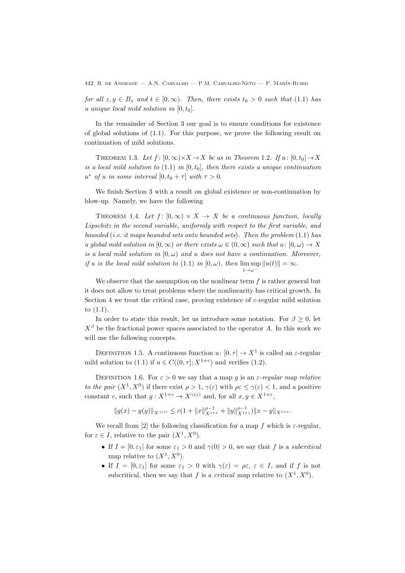
442 B. de Andrade — A.N. Carvalho — P.M. Carvalho-Neto — P. Marın-Rubio
for all z, y ∈ Bx and t ∈ [0,∞). Then, there exists t0 > 0 such that (1.1) has
a unique local mild solution in [0, t0].
In the remainder of Section 3 our goal is to ensure conditions for existence
of global solutions of (1.1). For this purpose, we prove the following result on
continuation of mild solutions.
Theorem 1.3. Let f : [0,∞)×X→X be as in Theorem 1.2. If u : [0, t0]→X
is a local mild solution to (1.1) in [0, t0], then there exists a unique continuation
u∗ of u in some interval [0, t0 + τ ] with τ > 0.
We finish Section 3 with a result on global existence or non-continuation by
blow-up. Namely, we have the following
Theorem 1.4. Let f : [0,∞) × X → X be a continuous function, locally
Lipschitz in the second variable, uniformly with respect to the first variable, and
bounded (i.e. it maps bounded sets onto bounded sets). Then the problem (1.1) has
a global mild solution in [0,∞) or there exists ω ∈ (0,∞) such that u : [0, ω)→ X
is a local mild solution in [0, ω) and u does not have a continuation. Moreover,
if u is the local mild solution to (1.1) in [0, ω), then lim supt→ω−
‖u(t)‖ =∞.
We observe that the assumption on the nonlinear term f is rather general but
it does not allow to treat problems where the nonlinearity has critical growth. In
Section 4 we treat the critical case, proving existence of ε-regular mild solution
to (1.1).
In order to state this result, let us introduce some notation. For β ≥ 0, let
Xβ be the fractional power spaces associated to the operator A. In this work we
will use the following concepts.
Definition 1.5. A continuous function u : [0, τ ]→ X1 is called an ε-regular
mild solution to (1.1) if u ∈ C((0, τ ];X1+ε) and verifies (1.2).
Definition 1.6. For ε > 0 we say that a map g is an ε-regular map relative
to the pair (X1, X0) if there exist ρ > 1, γ(ε) with ρε ≤ γ(ε) < 1, and a positive
constant c, such that g : X1+ε → Xγ(ε) and, for all x, y ∈ X1+ε,
‖g(x)− g(y)‖Xγ(ε) ≤ c(1 + ‖x‖ρ−1X1+ε + ‖y‖ρ−1X1+ε)‖x− y‖X1+ε .
We recall from [2] the following classification for a map f which is ε-regular,
for ε ∈ I, relative to the pair (X1, X0).
• If I = [0, ε1] for some ε1 > 0 and γ(0) > 0, we say that f is a subcritical
map relative to (X1, X0).
• If I = [0, ε1] for some ε1 > 0 with γ(ε) = ρε, ε ∈ I, and if f is not
subcritical, then we say that f is a critical map relative to (X1, X0).

Semilinear Fractional Differential Equations 443
• If I = (0, ε1] for some ε1 > 0 with γ(ε) = ρε, ε ∈ I, and f is not
subcritical or critical, then we say that f is a double-critical map relative
to (X1, X0).
• If I = [ε0, ε1] for some ε1 > ε0 > 0 with γ(ε0) > ρε0 and f is not
subcritical, critical or double critical, then we say that f is an ultra-
subcritical map relative to (X1, X0).
• If I = [ε0, ε1] for some ε1 > ε0 > 0 with γ(ε) = ρε, ε ∈ I, and if f is not
subcritical, critical, double critical or ultra-subcritical, then we say that
f is an ultra-critical map relative to (X1, X0).
Next theorem is the main result of Section 4 (the class F(ε, ρ, γ(ε), c, ν( · ), ξ)is specified).
Theorem 1.7. Let f ∈ F(ε, ρ, γ(ε), c, ν( · ), ξ). If v0 ∈ X1, there exist posi-
tive values r and τ0 such that for any u0 ∈ BX1(v0, r) there exists a continuous
function u( · , u0) : [0, τ0] → X1 with u(0) = u0, which is an ε-regular mild solu-
tion to the problem
(1.3)
cDαt u = Au+ f(t, u(t)), t > 0, α ∈ (0, 1),
u(0) = u0.
This solution satisfies
u ∈ C((0, τ0];X1+θ), 0 ≤ θ < γ(ε),
limt→0+
tαθ‖u(t, u0)‖X1+θ = 0, 0 < θ < γ(ε).
Moreover, for each θ0 < γ(ε) + ε− ρε there exists a constant C > 0 such that if
u0, w0 ∈ BX1(v0, r), then
tαθ‖u(t, u0)− u(t, w0)‖X1+θ ≤ C‖u0 − w0‖X1 for all t ∈ [0, τ0], 0 ≤ θ ≤ θ0.
In particular we obtain an existence theorem in X1 without the nonlinearity
being defined on X1. The main motivation to consider situations as in Theo-
rem 1.7 is the fact that if the only requirement on the nonlinear term is that
f : X1 → X0 be locally Lipschitz, we cannot ensure that problem (1.1) is well-
posed in an ε-regular sense. For example, taking f(u) = −2Au, which satisfies
f : X1 → X0 and is globally Lipschitz, we will have cDαt u = −Au, which is not
locally well-posed, in general. Hence, some extra conditions should be imposed
on f to guarantee the existence of solutions of the above problem.
As application we consider our abstract result in the framework of fractional
heat equations.
444 B. de Andrade — A.N. Carvalho — P.M. Carvalho-Neto — P. Marın-Rubio
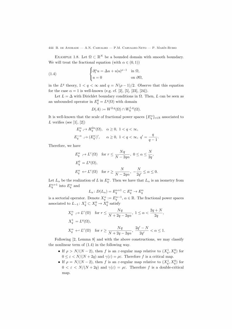
Example 1.8. Let Ω ⊂ RN be a bounded domain with smooth boundary.
We will treat the fractional equation (with α ∈ (0, 1))
(1.4)
∂αt u = ∆u+ u|u|ρ−1 in Ω,
u = 0 on ∂Ω,
in the Lq theory, 1 < q < ∞ and q = N(ρ− 1)/2. Observe that this equation
for the case α = 1 is well-known (e.g. cf. [2], [5], [23], [24]).
Let L = ∆ with Dirichlet boundary conditions in Ω. Then, L can be seen as
an unbounded operator in E0q = Lq(Ω) with domain
D(A) := W 2,q(Ω) ∩W 1,q0 (Ω).
It is well-known that the scale of fractional power spaces Eαq ε∈R associated to
L verifies (see [1], [2])
Eαq → H2αq (Ω), α ≥ 0, 1 < q <∞,
E−αq → (Eαq′)′, α ≥ 0, 1 < q <∞, q′ =
q
q − 1.
Therefore, we have
Eαq → Lr(Ω) for r ≤ Nq
N − 2qα, 0 ≤ α ≤ N
2q,
E0q = Lq(Ω),
Eαq ← Lr(Ω) for r ≥ N
N − 2qα, − N
2q′≤ α ≤ 0.
Let Lα be the realization of L in Eαq . Then we have that Lα is an isometry from
Eα+1q into Eαq and
Lα : D(Lα) = Eα+1q ⊂ Eαq → Eαq
is a sectorial operator. Denote Xαq := Eα−1q , α ∈ R. The fractional power spaces
associated to L−1 : X1q ⊂ X0
q → X0q satisfy
Xαq → Lr(Ω) for r ≤ Nq
N + 2q − 2qα, 1 ≤ α < 2q +N
2q,
X1q = Lq(Ω),
Xαq ← Lr(Ω) for r ≥ Nq
N + 2q − 2qα,
2q′ −N2q′
< α ≤ 1.
Following [2, Lemma 8] and with the above constructions, we may classify
the nonlinear term of (1.4) in the following way.
• If ρ > N/(N − 2), then f is an ε-regular map relative to (X1q , X
0q ) for
0 ≤ ε < N/(N + 2q) and γ(ε) = ρε. Therefore f is a critical map.
• If ρ = N/(N − 2), then f is an ε-regular map relative to (X1q , X
0q ) for
0 < ε < N/(N + 2q) and γ(ε) = ρε. Therefore f is a double-critical
map.

Semilinear Fractional Differential Equations 445
• If (N + 2)/N < ρ < N/(N − 2), then f is an ε-regular map relative to
(X1q , X
0q ) for 0 < ε0(ρ) < ε < 1/ρ, with
ε0(ρ) =1
ρ
(1− N
2
(1− 2
N(ρ− 1)
))> 0,
and γ(ε) = ρε. Therefore f is an ultra-critical map.
Applying Theorem 1.7, for each u0 ∈ Lq(Ω) we ensure the existence of an ε-regu-
lar solution to the above problem, starting at u0, for any ε ∈ (ε0(ρ), N/(N + 2q)).
Furthermore, for any 0 < θ < γ(N/(N + 2)) = 1 this solution verifies
tαθ‖u(t)‖X1+θ → 0 as t→ 0+,
tαθ‖u(t, u0)− u(t, v0)‖X1+θ ≤ C‖u0 − v0‖Lq , 0 < t < τ(u0, v0).
In Section 5 we consider the problem of comparison and positive solutions.
We start this with the linear version of (1.1); particularly, we establish the equiv-
alence between the positivity of the families Eα(tαA)t≥0 and Eα,α(tαA)t≥0with the positivity of the function λ 7→ (λα−A)−1 (see Propositions 5.1 and 5.3
below). With respect to the semilinear problem (1.1), we establish the following
result on positive solutions.
Theorem 1.9. Let (X,≤X) be an ordered Banach space and suppose that the
families Eα(tαA)t≥0 and Eα,α(tαA)t≥0 are increasing. If 0 ≤X f(t, x) for
almost every t ∈ [0, t0) and for all x ∈ X with 0 ≤X x, then 0 ≤X u0 implies that
the local mild solution uf (t, u0) is positive, i.e. 0 ≤X uf (t, u0) for all t ∈ [0, t0].
This allows us to conclude the following comparison result.
Theorem 1.10. Let (X,≤X) be an ordered Banach space and suppose that
the families Eα(tαA)t≥0 and Eα,α(tαA)t≥0 are increasing.
(a) Let u0, u1 ∈ X be given, and assume that there exist t0, t1 ∈ [0,∞) such
that uf (t, ui)i=0,1 are local mild solutions in [0, ti], i ∈ 0, 1, tocDαt u(t) = Au(t) + f(t, u(t)), t > 0,
u(0) = ui ∈ X.
Then, if t∗ = mint0, t1, f(t, · ) is increasing for almost every t ∈ [0, t∗),
and u1 ≤X u0, it holds that uf (t, u1) ≤X uf (t, u0) for all t ∈ [0, t∗].
(b) Consider functions f0 and f1, and u0 ∈ X, and assume that there exist
t0, t1 ∈ [0,∞) such that ufi(t, u0)i=0,1 are local mild solutions in [0, ti],
i ∈ 0, 1, tocDαt u(t) = Au(t) + fi(t, u(t)), t > 0,
u(0) = u0 ∈ X.
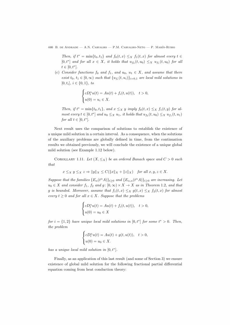
446 B. de Andrade — A.N. Carvalho — P.M. Carvalho-Neto — P. Marın-Rubio
Then, if t∗ = mint0, t1 and f0(t, x) ≤X f1(t, x) for almost every t ∈[0, t∗] and for all x ∈ X, it holds that uf0(t, u0) ≤X uf1(t, u0) for all
t ∈ [0, t∗].
(c) Consider functions f0 and f1, and u0, u1 ∈ X, and assume that there
exist t0, t1 ∈ [0,∞) such that ufi(t, ui)i=0,1 are local mild solutions in
[0, ti], i ∈ 0, 1, tocDαt u(t) = Au(t) + fi(t, u(t)), t > 0,
u(0) = ui ∈ X.
Then, if t∗ = mint0, t1, and x ≤X y imply f0(t, x) ≤X f1(t, y) for al-
most every t ∈ [0, t∗] and u0 ≤X u1, it holds that uf0(t, u0) ≤X uf1(t, u1)
for all t ∈ [0, t∗].
Next result uses the comparison of solutions to establish the existence of
a unique mild solution in a certain interval. As a consequence, when the solutions
of the auxiliary problems are globally defined in time, from the continuation
results we obtained previously, we will conclude the existence of a unique global
mild solution (see Example 1.12 below).
Corollary 1.11. Let (X,≤X) be an ordered Banach space and C > 0 such
that
x ≤X y ≤X z ⇒ ‖y‖X ≤ C(‖x‖X + ‖z‖X) for all x, y, z ∈ X.
Suppose that the families Eα(tαA)t≥0 and Eα,α(tαA)t≥0 are increasing. Let
u0 ∈ X and consider f1, f2 and g : [0,∞)×X → X as in Theorem 1.2, and that
g is bounded. Moreover, assume that f1(t, x) ≤X g(t, x) ≤X f2(t, x) for almost
every t ≥ 0 and for all x ∈ X. Suppose that the problemscDαt u(t) = Au(t) + fi(t, u(t)), t > 0,
u(0) = u0 ∈ X
for i = 1, 2 have unique local mild solutions in [0, t∗] for some t∗ > 0. Then,
the problem cDαt u(t) = Au(t) + g(t, u(t)), t > 0,
u(0) = u0 ∈ X.
has a unique local mild solution in [0, t∗].
Finally, as an application of this last result (and some of Section 3) we ensure
existence of global mild solution for the following fractional partial differential
equation coming from heat conduction theory:
Semilinear Fractional Differential Equations 447
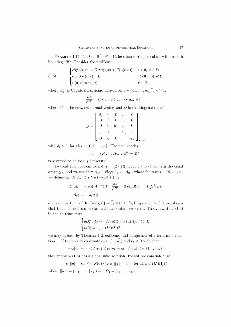
Example 1.12. Let Ω ⊂ RN , N ∈ N, be a bounded open subset with smooth
boundary ∂Ω. Consider the problem
(1.5)
c∂αt u(t, x) = D∆u(t, x) + F (u(t, x)), t > 0, x ∈ Ω,
∂u/∂−→v (t, x) = 0, t > 0, x ∈ ∂Ω,
u(0, x) = u0(x), x ∈ Ω.
where c∂αt is Caputo’s fractional derivative, u = (u1, . . . , un)>, n ≥ 1,
∂u
∂−→v= (〈∇u1,−→v 〉, . . . , 〈∇un,−→v 〉)>,
where −→v is the outward normal vector, and D is the diagonal matrix
D =
d1 0 0 . . . 0
0 d2 0 . . . 0
0 0 d3 . . . 0...
......
. . ....
0 0 0 . . . dn
n×n
with di > 0, for all i ∈ 0, 1, . . . , n. The nonlinearity
F = (F1, . . . , Fn) : Rn → Rn
is assumed to be locally Lipschitz.
To treat this problem we set X = (Lq(Ω))n, for 1 < q < ∞, with the usual
order ≤X and we consider AD = diag(A1, . . . An), where for each i ∈ 0, . . . , nwe define Ai : D(Ai) ⊂ Lq(Ω)→ Lq(Ω) by
D(Ai) =
φ ∈W 2,q(Ω) :
∂φ
∂−→v= 0 on ∂Ω
=: W 2,q
N (Ω);
Aiφ = − di∆φ
and suppose that infRe(σ(AD)) = d1 < 0. In [6, Proposition 2.8] it was shown
that this operator is sectorial and has positive resolvent. Then, rewriting (1.5)
in the abstract formcDαt u(t) = −ADu(t) + F (u(t)), t > 0,
u(0) = u0 ∈ (Lq(Ω))n,
we may ensure, by Theorem 1.2, existence and uniqueness of a local mild solu-
tion u. If there exist constants c0 ∈ [0,−d1) and c1 ≥ 0 such that
−c0|ui| − c1 ≤ Fi(u) ≤ c0|ui|+ c1 for all i ∈ 1, . . . , n,
then problem (1.5) has a global mild solution. Indeed, we conclude that
−c0|||u||| − C1 ≤X F (u) ≤X c0|||u|||+ C1 for all u ∈ (Lq(Ω))n,
where |||u||| := (|u1|, . . . , |un|) and C1 = (c1, . . . , c1).

448 B. de Andrade — A.N. Carvalho — P.M. Carvalho-Neto — P. Marın-Rubio
Since the problemscDαt u(t) = −ADu(t)− c0|||u(t)||| − C1, t > 0,
u(0) = u0 ∈ (Lq(Ω))n,
and cDαt u(t) = −ADu(t) + c0|||u(t)|||+ C1, t > 0,
u(0) = u0 ∈ (Lq(Ω))n,
have global mild solutions (by using Theorem 1.4), we conclude by Corollary 1.11
and Theorems 1.3 and 1.4 that (1.5) possesses a unique global mild solution.
2. Preliminary results
Let (X, ‖ · ‖) be a complex Banach space. As usual, for a linear operatorA, we
denote by D(A) the domain of A, by σ(A) its spectrum, while ρ(A) := C−σ(A)
is the resolvent set of A. Moreover, we denote by L(Y, Z) the space of all
bounded linear operators between two normed spaces Y and Z with the operator
norm ‖ · ‖L(Y,Z). We abbreviate this notation to L(Y ) when Y = Z. When no
confusion arise, we write ‖T‖L(Y ) as ‖T‖ for every T ∈ L(Y ). Finally, for β ≥ 0
we denote by Xβ the fractional power spaces associated to the operator A, being
X0 = X and X1 = D(A).
The aim of this section is to present the basic tools we will use in this man-
uscript. Our results include the classical theory of the Mittag-Leffler function
that is closely related to the solutions of the fractional differential equations.
2.1. Mittag–Leffler functions and sectorial operators. We start with
a generalization of the Cauchy representation for semigroups associated to sec-
torial operators. To this end we recall that given ε > 0 and θ ∈ (π/2, π), the
Hankel path Ha = Ha(ε, θ) is the path given by Ha = Ha1 +Ha2−Ha3, where
Hai are such that
(2.1)
Ha1 := teiθ : t ∈ [ε,∞),
Ha2 := εeit : t ∈ [−θ, θ],
Ha3 := te−iθ : t ∈ [ε,∞).
Lemma 2.1. Consider α ∈ (0, 1) and suppose that A : D(A) ⊂ X → X is
a sectorial operator. Then, the functions
Eα(tαA) :=1
2πi
∫Ha
eλtλα−1(λα −A)−1dλ, t ≥ 0,
Eα,α(tαA) :=t1−α
2πi
∫Ha
eλt(λα −A)−1dλ, t ≥ 0

Semilinear Fractional Differential Equations 449
(where Ha is given by (2.1)) are well defined. Furthermore, there exists a con-
stant M > 0 such that
‖Eα(tαA)‖ ≤M and ‖Eα,α(tαA)‖ ≤M for all t ≥ 0.
Proof. Let φ ∈ (π/2, π), Sφ be the sector associated with the sectorial
operator A and choose arbitrary values ε > 0 and θ ∈ (π/2, φ]. We will estimate
the function ‖Eα(tαA)‖ on each Hai, according to definition (2.1), for any t > 0.
Just observe that for each fixed t 6= 0, if we assume that ε = 1/t, then
• On Ha1, it holds that∥∥∥∥ 1
2πi
∫Ha1
eλtλα−1(λα −A)−1dλ
∥∥∥∥≤ 1
2π
∥∥∥∥∫ ∞ε
etseiθ
(seiθ)α−1((seiθ)α −A)−1eiθ ds
∥∥∥∥and using that if λ = seiθ ∈ Ha(ε, θ) ⊂ Sφ, then λα ∈ Sφ, we obtain by
the sectorial property that∥∥∥∥ 1
2πi
∫Ha1
eλtλα−1(λα −A)−1dλ
∥∥∥∥ ≤ N
2π
∫ ∞ε
ets cos(θ)|(seiθ)|−1ds
≤ N
2πε
∫ ∞ε
ets cos(θ)ds =Necos(θ)
−2π cos(θ).
• On Ha2, we have that∥∥∥∥ 1
2πi
∫Ha2
eλtλα−1(λα −A)−1dλ
∥∥∥∥=
1
2π
∥∥∥∥∫ θ
−θetεe
is
(εeis)α−1((εeis)α −A)−1iεeisds
∥∥∥∥≤ N
2π
∫ θ
−θetε cos(s) ds ≤ θNe
π.
• On Ha3 we proceed in the same way as in Ha1.
Taking M as the maximum over all the bounds obtained above, we deduce
that ‖Eα(Atα)‖ is well defined for each t ≥ 0.
Now we shall seek a uniform bound for the function ‖Eα(Atα)‖ for all t ≥ 0.
For this, just observe that if ε < ε′ and π/2 < θ′ < θ < φ and we take Ha =
Ha(ε, θ) and Ha′ = Ha(ε′, θ′), we obtain the equality
1
2πi
∫Ha
eλtλα−1(λα −A)−1dλ =1
2πi
∫Ha′
eλtλα−1(λα −A)−1dλ for all t ≥ 0.
This is enough to justify that the estimate obtained before is uniform on t > 0.
To verify the boundedness for t = 0, we observe that making a change of variables
Eα(tαA) =1
2πi
∫Ha
eλλα−1(λα −Atα)−1 dλ, t ≥ 0,

450 B. de Andrade — A.N. Carvalho — P.M. Carvalho-Neto — P. Marın-Rubio
and therefore, using the dominated convergence theorem, we conclude that
Eα(0αA) is the identity operator.
A similar procedure proves that ‖Eα,α(Atα)‖ ≤M for all t ∈ [0,∞).
Next result give us information on the Mittag–Leffler families in the fractional
power spaces Xβ , β ≥ 0, associated to the sectorial operator A.
Lemma 2.2. Consider α ∈ (0, 1), 0 ≤ β ≤ 1, and suppose that A : D(A) ⊂X0 → X0 is a sectorial operator. Then, there exists a constant M > 0 such that
‖Eα(tαA)x‖Xβ ≤Mt−αβ‖x‖X0
and
‖tα−1Eα,α(tαA)x‖Xβ ≤Mtα(1−β)−1‖x‖X0
for all t > 0.
Proof. We have that
‖Eα(tαA)x‖Xβ =
∥∥∥∥ 1
2πi
∫Ha
eλtλα−1Aβ(λα −A)−1x dλ
∥∥∥∥X0
≤ t−α
2π
∥∥∥∥∫Ha
eλλα−1Aβ((λ/t)α −A)−1x dλ
∥∥∥∥X0
≤ t−αβ(C
2π
∫Ha
|eλλαβ−1| d|λ|)‖x‖X0 .
Hence, it is sufficient to choose M > 0 such that
C
2π
∫Ha
|eλλαβ−1| d|λ| ≤M.
By a similar procedure one may prove the second estimate.
Our goal now is to establish an expression for Mittag–Leffler functions as-
sociated to sectorial operators similar to the second fundamental limit for semi-
groups. For this, we recall the Post–Widder inversion formula, which can be
found in [26]. This expression will be very useful to our following results.
Lemma 2.3 (Post–Widder). Let u : [0,∞) → X be a continuous function
such that u(t) = O(exp(ωt)) as t→∞ for some ω ∈ R and let u be the Laplace
transform of u. Then
u(t) = limn→∞
(−1)n
n!
(n
t
)n+1(dn
dλnu
)(n
t
),
uniformly on compact sets of (0,∞).

Semilinear Fractional Differential Equations 451
Proposition 2.4. Consider A : D(A) ⊂ X → X a sectorial operator and
α ∈ (0, 1). Let Eα(tαA)t≥0 and Eα,α(tαA)t≥0 be the Mittag–Leffler families
associated to A. Then, for each x ∈ X we have
(2.2) Eα(tαA)x = limn→∞
1
n!
n+1∑k=1
bαk,n+1
((n
t
)α((n
t
)α−A
)−1)kx,
and
(2.3) tα−1Eα,α(tαA)u0 = limn→∞
1
n!
n∑k=1
αkbαk,n
(n
t
)αk+1((n
t
)α−A
)−(k+1)
x,
uniformly on compact sets of (0,∞), where the positive real numbers bαk,n are
defined by
(2.4)
bα1,1 = 1,
bαk,n = (n− 1− αk)bαk,n−1 + α(k − 1)bαk−1,n−1, if 1 ≤ k ≤ nand n = 2, 3, . . . ,
bαk,n = 0, if k > n
and n = 1, 2, . . .
Proof. By Lemma 2.1 there exists M ≥ 1 such that ‖Eα(tαA)‖ ≤ M and
‖Eα,α(tαA)‖ ≤M for all t ≥ 0. By induction in n, we obtain for Reλ > 0 that
dn
dλn(λα−1(λα−A)−1) = (−1)nλ−(n+1)
n+1∑k=1
bαk,n+1[λα(λα−A)−1]k, n = 1, 2, . . .
Furthermore, for each x ∈ X the function u(t) = Eα(tαA)x is such that
u(λ) = λα−1(λα −A)−1x.
Hence, (2.2) follows by Lemma 2.3.
On the other hand, to prove (2.3), observe that
dn
dλn(λα −A)−1 = (−1)nλ−n
n∑k=1
αkbαk,nλαk(λα −A)−(k+1), n = 1, 2, . . .
and for each x ∈ X, the function v(t) = tα−1Eα,α(tαA)x verifies v(λ) = (λα −A)−1x. Using again Lemma 2.3, the proof is finished.
2.2. Ordered Banach spaces. We recall briefly the basic properties of an
order on a Banach space X, in order to develop our comparison results.
Definition 2.5. An ordered Banach space is a couple (X,≤X) where X is
a Banach space and ≤X is an order relation in X such that for every x, y, z ∈ Xand for any scalar λ ≥ 0, it holds that
(a) x ≤X y implies x+ z ≤X y + z;
(b) x ≤X y implies λx ≤X λy;

452 B. de Andrade — A.N. Carvalho — P.M. Carvalho-Neto — P. Marın-Rubio
(c) the positive cone C = x ∈ X : 0 ≤X x is closed in X.
Remark 2.6. Observe that x ≤X y is equivalent to 0 ≤X y−x. Furthermore,
x ≤X 0 if and only if 0 ≤X −x.
Example 2.7. Consider 1 ≤ p ≤ ∞. The Banach spaces Lp(Ω) and C(Ω)
with the order “f ≤ g if and only if f(x) ≤ g(x) almost everywhere” are ordered
Banach spaces.
Definition 2.8. Suppose that (X,≤X) and (Y,≤Y ) are ordered Banach
spaces. A function T : D(T ) ⊂ X → Y is called increasing if x ≤X y implies
Tx ≤Y Ty. T is called positive if 0 ≤X x implies 0 ≤Y Tx, for all x, y ∈ D(T ).
Lemma 2.9. Let (X,≤X) be an ordered Banach space and consider f ∈L1(t0, t1;X) such that 0 ≤X f(t) for almost every t ∈ (t0, t1). Then
0 ≤X∫ t1
t0
f(s) ds.
3. Local well posedness
We start this section with a proof of our result on local existence and unique-
ness of mild solutions to (1.1).
Proof of Theorem 1.2. Given u0 ∈ X, let Bu0(r) be the open ball with
center u0 and radius r > 0 and L = L(Bu0(r)) be the Lipschitz constant of f
associated to Bu0(r). Fix β ∈ (0, r) and choose t0 > 0 such that
(M/α)(Lβ + C)tα0 ≤ β/2 and ‖Eα(Atα)u0 − u0‖ ≤ β/2 for all t ∈ [0, t0].
where M = supt∈[0,∞)
‖Eα,α(Atα)‖ and C = supt∈[0,t0]
‖f(s, u0)‖. Consider
K := u ∈ C([0, t0];X) : u(0) = u0 and ‖u(t)− u0‖ ≤ β for all t ∈ [0, t0]
and define the operator T on K by
T (u(t)) = Eα(tαA)u0 +
∫ t
0
(t− s)α−1Eα,α((t− s)αA)f(s, u(s)) ds.
If u ∈ K, then T (u(0)) = u0 and T (u(t)) ∈ C([0, t0];X). Furthermore, we have
that
‖T (u(t))− u0‖ ≤‖Eα(Atα)u0 − u0‖
+
∫ t
0
(t− s)α−1M(‖f(s, u(s))− f(s, u0)‖+ ‖f(s, u0)‖) ds
≤‖Eα(Atα)u0 − u0‖+ (M/α)(Lβ + C)tα0 ≤β
2+β
2= β,
that is, T (K) ⊂ K. Now, if u, v ∈ K, we see that
‖T (u(t))− T (v(t))‖ ≤∫ t
0
(t− s)α−1M‖f(s, u(s))− f(s, v(s))‖ ds
Semilinear Fractional Differential Equations 453
≤ LMtα0α
sups∈[0,t0]
‖u(s)− v(s)‖
≤ 1
2sup
s∈[0,t0]‖u(s)− v(s)‖.
So, by the Banach contraction principle we have that T has a unique fixed point
in K. We will denote this fixed point by w.
Uniqueness of local mild solution to (1.1) follows from the Singular Gronwall
Inequality (see [9, Lemma 7.1.1, p. 188]). Therefore, we obtain that the solution
ω is the unique continuous function that satisfies the integral equation and this
finishes the proof.
Definition 3.1. Let u : [0, t0]→ X be a local mild solution in [0, t0] to (1.1).
If t1 > t0 and v : [0, t1] → X is a local mild solution to (1.1) in [0, t1], then we
say that v is a continuation of u in [0, t1].
The remainder of this paragraph will be devoted to the problem of continu-
ation of local mild solutions and existence of global mild solutions of (1.1).
Proof of Theorem 1.3. Let u : [0, t0] → X be the local mild solution
to (1.1) in [0, t0]. Since f is locally Lipschitz, there exist r > 0, an open ball
B = B(u(t0)) with center in u(t0) and radius r, and L = Lu(t0) the Lipschitz
constant of f associated to B. Fix β ∈ (0, r) and choose τ > 0 such that the
following conditions are satisfied:
• ‖Eα(Atα)u0 − Eα(At0α)u0‖ ≤ β/4,
• (M/α)(Lβ + C)τα ≤ β/4, (MD/α)[tα − (t− t0)α − tα0 ] ≤ β/4,
•∫ t0
0
(t0 − s)α−1‖[Eα,α(A(t− s)α)− Eα,α(A(t0 − s)α)]f(s, u(s))‖ ds ≤ β
4
for all t ∈ [t0, t0 + τ ], where
C = sups∈[0,t0]
‖f(s, u(t0))‖,
D = sups∈[0,t0]
‖f(s, u(s))‖,
M = max
sup
t∈[0,∞)
‖Eα,α(Atα)‖, supt∈[0,∞)
‖Eα(Atα)‖.
Consider
K := w ∈ C([0, t0 + τ ];X) : w(t) = u(t) for all t ∈ [0, t0]
and ‖w(t)− u(t0)‖ ≤ β for all t ∈ [t0, t0 + τ ]
and T : K → C([0, t0 + τ ];X) given by
T (w(t)) = Eα(tαA)u0 +
∫ t
0
(t− s)α−1Eα,α((t− s)αA)f(s, u(s)) ds.

454 B. de Andrade — A.N. Carvalho — P.M. Carvalho-Neto — P. Marın-Rubio
We check that T (K) ⊂ K.
(a) If w ∈ K, then w(t) = u(t) in [0, t0] with u the local mild solution to
(1.1) in [0, t0]. So, if t ∈ [0, t0],
T (w(t)) =Eα(tαA)u0 +
∫ t
0
(t− s)α−1Eα,α((t− s)αA)f(s, w(s)) ds
=Eα(tαA)u0 +
∫ t
0
(t− s)α−1Eα,α((t− s)αA)f(s, u(s)) ds = u(t).
(b) If t ∈ [t0, t0 + τ ], then
‖T (w(t)) − u(t0)‖ ≤ ‖Eα(tαA)u0 − Eα(t0αA)u0‖
+
∥∥∥∥ ∫ t
0
(t− s)α−1Eα,α((t− s)αA)f(s, w(s)) ds
−∫ t0
0
(t0 − s)α−1Eα,α((t0 − s)αA)f(s, w(s)) ds
∥∥∥∥≤I1 + I2 + I3 + I4 ≤ β,
where
I1 = ‖Eα(tαA)u0 − Eα(t0αA)u0‖ ≤
β
4,
I2 =
∥∥∥∥ ∫ t
t0
(t− s)α−1Eα,α((t− s)αA)f(s, w(s)) ds
∥∥∥∥ ≤ β
4,
I3 =
∥∥∥∥ ∫ t0
0
[(t− s)α−1 − (t0 − s)α−1]Eα,α((t− s)αA)f(s, w(s)) ds
∥∥∥∥ ≤ β
4,
I4 =
∥∥∥∥ ∫ t0
0
(t0 − s)α−1[Eα,α((t− s)αA)− Eα,α((t0 − s)αA)]f(s, w(s)) ds
∥∥∥∥ ≤ β
4.
By similar computations, we conclude that, for every t ∈ [0, t0 + τ ],
‖T (ω(t))− T (v(t))‖ ≤ LMτα
αsup
s∈[0,t0+τ ]‖ω(s)− v(s)‖
≤ 1
2sup
s∈[0,t0+τ ]‖ω(s)− v(s)‖
for all u, v ∈ K. Therefore, by the Banach contraction principle, we conclude
that there exists a unique fixed point u∗ ∈ K of the integral equation. As in the
proof of Theorem 1.2, it is not difficult to see that u∗ is the unique continuous
continuation of u in [0, t0 + τ ].
The following result will be useful in the proof of Theorem 1.4.
Lemma 3.2. Consider ω ∈ (0,∞), u : [0, ω) → X a bounded continuous
function, and f : [0,∞) × X → X continuous and bounded. If tn ⊂ [0, ω)
Semilinear Fractional Differential Equations 455
satisfies limn tn = ω, then
limn
∫ tn
0
(tn − r)α−1‖[Eα,α(A(tn − rα))− Eα,α(A(w − rα))]f(r, u(r))‖ dr = 0.
Proof. Let M = supt∈[0,∞)
‖Eα,α(Atα)‖ and K = sups∈[0,ω)
‖f(s, u(s))‖. Given
ε > 0, fix γ ∈ (0, ω) such that
(ω − γ)α
αMK ≤ ε
2.
Now, choose N ∈ N such that
• tn > γ for all n ≥ N ;
•∫ γ
0
(tn − r)α−1‖[Eα,α(A(tn − rα))− Eα,α(A(w − rα))]f(r, u(r))‖ dr < ε
2for all n ≥ N .
Hence, we conclude that for n ≥ N ,∫ tn
0
(tn − r)α−1‖[Eα,α(A(tn − rα))− Eα,α(A(w − rα))]f(r, u(r))‖ dr
≤ ε
2+
∫ tn
γ
(tn − r)α−1MK dr ≤ ε
2+
(ω − γ)α
αMK ≤ ε.
Proof of Theorem 1.4. ConsiderH := τ ∈ [0,∞) : there exists uτ : [0, τ ]
→ X unique local mild solution to (1.1) in [0, τ ]. If supH = w, we can consider
a continuous function u : [0, ω) → X that is a local mild solution to (1.1) in
[0, ω). If ω =∞, then u is a global mild solution in [0,∞). Otherwise, if ω <∞we will prove that lim sup
t→ω|u(t)| = ∞. By contradiction, suppose that there
exists K <∞ such that ‖u(t)‖ ≤ K for all t ∈ [0, ω). Therefore, it follows from
Lemma 3.2 that if tn ⊂ [0, ω) is a sequence that converges to ω, given ε > 0,
there exists N ∈ N, such that, if m, n ≥ N, we have
‖Eα(tαnA)u0 − Eα(tαmA)u0‖ ≤ε
5,
|tn − tm|αMK
α≤ ε
5,
|tαn − (tn − tm)α − tαm|MK
α≤ ε
5,
∫ tn
0
(tn − r)α−1‖[Eα,α((tn − r)αA)− Eα,α((w − r)αA)]f(r, u(r))‖ dr ≤ ε
5,∫ tm
0
(tm − r)α−1‖[Eα,α((tm − r)αA)− Eα,α((w − r)αA)]f(r, u(r))‖ dr ≤ ε
5,
where
K = supt∈[0,ω)
‖f(t, u(t))‖, M = max supt∈[0,∞)
‖Eα,α(Atα)‖, supt∈[0,∞)
‖Eα(Atα)‖.

456 B. de Andrade — A.N. Carvalho — P.M. Carvalho-Neto — P. Marın-Rubio
Hence, for n,m ≥ N and assuming, without loss of generality, that tn > tm, it
follows from the estimate
‖u(tn)− u(tm)‖ ≤ ‖Eα(tαnA)u0 − Eα(tαmA)u0‖+ I1 + I2 + I3,
where
I1 =
∫ tn
tm
(tn − r)α−1‖Eα,α((tn − r)αA)f(r, u(r))‖ dr ≤ |tn − tm|αMK
α,
I2 =
∫ tm
0
(tn − r)α−1‖[Eα,α((tn − r)αA)− Eα,α((tm − r)αA)]f(r, u(r))‖ dr
≤∫ tm
0
(tn − r)α−1‖[Eα,α((tn − r)αA)− Eα,α((ω − r)αA)]f(r, u(r))‖ dr
+
∫ tm
0
(tn − r)α−1‖[Eα,α((tm − r)αA)− Eα,α((ω − r)αA)]f(r, u(r))‖ dr
≤∫ tn
0
(tn − r)α−1‖[Eα,α((tn − r)αA)− Eα,α((ω − r)αA)]f(r, u(r))‖ dr
+
∫ tm
0
(tm − r)α−1‖[Eα,α((tm − r)αA)− Eα,α((ω − r)αA)]f(r, u(r))‖ dr
and
I3 =
∫ tm
0
|[(tn − s)α−1 − (tm − s)α−1]| ‖Eα,α((tm − s)αA)f(s, u(s))‖ ds
≤ |tαn − (tn − tm)α − tαm|MK
α,
that ‖u(tn) − u(tm)‖ ≤ ε. This computation shows that u(tn) is a Cauchy
sequence and therefore it has a limit, ut ∈ X. Then, we may extend u over [0, ω]
obtaining the equality
u(t) = Eα(tαA)u0 +
∫ t
0
(t− s)α−1Eα,α((t− s)αA)f(s, u(s)) ds
for all t ∈ [0, ω]. With this, by Theorem 1.3, we can extend the solution to some
bigger interval, which is a contradiction with the definition of ω.
Corollary 3.3. Let f : [0,∞)×X → X be as in Theorem 1.4 and suppose
that there exists a constant K > 0 such that if ‖u0‖ ≤ K, then the solutions
to (1.1), while exists, are bounded by K. Then (1.1) possesses a unique global
mild solution.
4. Critical nonlinearities
Following the notation of [2], we consider the following class of nonlinearities:
let ε, γ(ε), ξ, ζ, c, and δ be positive constants, and a function ν with values in
[0, δ) and limt→0+ ν(t) = 0. Define F(ε, ρ, γ(ε), c, ν( · ), ξ, ζ) as the family of

Semilinear Fractional Differential Equations 457
functions f such that, for t ≥ 0, f(t, · ) is an ε-regular map relative to the pair
(X1, X0), satisfying, for all x, y ∈ X1+ε,
‖f(t, x)− f(t, y)‖Xγ(ε) ≤ c(‖x‖ρ−1X1+ε + ‖y‖ρ−1X1+ε + ν(t)t−ζ)‖x− y‖X1+ε ,
‖f(t, x)‖Xγ(ε) ≤, c(‖x‖ρX1+ε + ν(t)t−ξ).
Without loss of generality we may assume that the function ν is non-decre-
asing. We will suppose that 0 ≤ ζ ≤ α(γ(ε)− ε) and 0 ≤ ξ ≤ αγ(ε), α ∈ (0, 1).
In most cases in the arguments below we will fix the parameters ε, γ(ε), ρ, ξ, ζ
and c, and we will denote the class F defined above by F(ν( · )).As immediate consequence of Lemma 2.2 we have that if 0 ≤ θ, β ≤ 1, then
tα(1+θ−β)‖Eα(tαA)x‖X1+θ ≤M‖x‖Xβ ,(4.1)
tα(θ−β)+1‖tα−1Eα,α(tαA)x‖X1+θ ≤M‖x‖Xβ .
To prove Theorem 1.7 we need some previous results.
Lemma 4.1. Consider α ∈ (0, 1), θ ∈ [0, 1], and a sectorial operator A. The
operators tαθEα(tαA) : X1 → X1+θt>0 are bounded linear operators satisfying
‖tαθEα(tαA)‖L(X1,X1+θ) ≤M,
with M > 0 independent of t. Moreover, given a compact subset J of X1, we
have
limt→0+
supx∈J‖tαθEα(tαA)x‖X1+θ = 0.
Proof. The fact that ‖tαθEα(tαA)‖L(X1,X1+θ) ≤M follows from (4.1). For
the remaining part it suffices to observe that the operators tαEα(tαA) : X1 →X1+α are uniformly bounded in t, that
limt→0+
‖tαEα(tαA)x‖X1+α = 0,
for x ∈ X1+α, and that Xα is a dense subset of X1.
Let B : (0,∞)× (0,∞)→ (0,∞) be the beta function given by
B(a, b) =
∫ 1
0
(1− x)a−1xb−1 dx.
For ζ ≥ 0, define
Bθε(ζ) = sup
0≤η≤θB(α(γ(ε)− η), 1− ζ),B(α(γ(ε)− η), 1− αρε).
Lemma 4.2. With the above notation, let f ∈F(ν( · )). If u∈C((0, τ ];X1+ε),
then, for all 0 ≤ θ < γ(ε), we have that
tαθ∥∥∥∥∫ t
0
(t− s)α−1Eα,α((t− s)αA)f(s, u(s)) ds
∥∥∥∥X1+θ
≤McBθε(ξ)(ν(t)tαγ(ε)−ξ + λ(t)ρtα(γ(ε)−ρε))
458 B. de Andrade — A.N. Carvalho — P.M. Carvalho-Neto — P. Marın-Rubio
for 0 < t ≤ τ , where λ(t) = sups∈(0,t]
sαε‖u(s)‖X1+ε.
Proof. Indeed, we have that
tαθ∫ t
0
‖(t− s)α−1Eα,α((t− s)αA)f(s, u(s))‖X1+θ ds
≤Mtαθ∫ t
0
(t− s)α(γ(ε)−θ)−1c(ν(s)s−ξ + ‖u(s)‖ρX1+ε) ds
≤Mcν(t)tαθ∫ t
0
(t− s)α(γ(ε)−θ)−1s−ξ ds
+Mctαθ∫ t
0
(t− s)α(γ(ε)−θ)−1s−αρε(sαε‖u(s)‖X1+ε)ρ ds
≤Mcν(t)tαθ−ξ+α(γ(ε)−θ)∫ 1
0
(1− s)α(γ(ε)−θ)−1s−ξ ds
+Mcλ(t)ρtαθ−αρε+α(γ(ε)−θ)∫ 1
0
(t− s)α(γ(ε)−θ)−1s−αρε ds
≤McBθε(ξ)(ν(t)tαγ(ε)−ξ + λ(t)ρtα(γ(ε)−ρε)),
which concludes the proof.
Lemma 4.3. With the above notation, let f ∈ F(ν( · )) and consider u, v ∈C((0, τ ];X1+ε) such that tαε‖u(t)‖X1+ε ≤ µ and tαε‖v(t)‖X1+ε ≤ µ for some
µ > 0. Then, for all 0 ≤ θ < γ(ε) < 1, we have
tαθ∥∥∥∥∫ t
0
(t− s)α−1Eα,α((t− s)αA)(f(s, u(s))− f(s, v(s))) ds
∥∥∥∥X1+θ
≤McBθε(ζ + αε)[ν(t)tα(γ(ε)−θ)−ζ + 2µρ−1tα(γ(ε)+ε−θ−ρε)]
× sup0<s≤τ
sαε‖u(s)− v(s)‖X1+ε .
Proof. It follows from the ε-regularity property of f that
tαθ∫ t
0
‖(t− s)α−1Eα,α((t− s)αA)(f(s, u(s))− f(s, v(s)))‖X1+θ ds
≤Mtαθ∫ t
0
(t− s)α(γ(ε)−θ)−1‖f(s, u(s))− f(s, v(s))‖Xγ(ε) ds
≤Mctαθ∫ t
0
(t− s)α(γ(ε)−θ)−1‖u(s)− v(s)‖X1+ε
× (‖u(s)‖ρ−1X1+ε + ‖v(s)‖ρ−1X1+ε + ν(s)s−ζ) ds
≤Mcν(t)tαθ∫ t
0
(t− s)α(γ(ε)−θ)−1s−ζ−αεsαε‖u(s)− v(s)‖X1+ε ds
+Mctαθ∫ t
0
(t− s)α(γ(ε)−θ)−1s−αρε
Semilinear Fractional Differential Equations 459
× [(sαε‖u(s)‖X1+ε)ρ−1 + (sαε‖v(s)‖X1+ε)ρ−1]sαε‖u(s)− v(s)‖x1+ε ds
≤ [ν(t)tα(γ(ε)−θ)−ζ + 2µρ−1tα(γ(ε)+ε−θ−ρε)]
×McBθε(ζ + αε) sup
0≤s≤τsαε‖u(s)− v(s)‖X1+ε .
Now we may prove the main result of this section.
Proof of Theorem 1.7. Define µ by
McBεεµρ−1 =
1
8,
where Bθε := maxBθ
ε(ξ),Bθε(ζ + αε) and choose r = r(µ,M) > 0 such that
r =µ
4M=
1
4M(8cMBεε)
1/(ρ−1) .
For v0 fixed, choose τ0 ∈ (0, 1] such that ν(t) < δ for all t ∈ (0, τ0],
‖tαεEα(tαA)v0‖X1+ε ≤ µ
2if 0 ≤ t ≤ τ0,
and
McδBεε = min
µ
8,
1
4
.
Consider
K(τ0) =
u ∈ C((0, τ0];X1+ε) : sup
t∈(0,τ0]tαε‖u(t)‖X1+ε ≤ µ
with norm
‖u‖K(τ0) = supt∈(0,τ0]
tαε‖u(t)‖X1+ε .
Suppose that u0 ∈ X1 with ‖u0 − v0‖X1 < r and define on K(τ0) the map
Tu(t) = Eα(tαA)u0 +
∫ t
0
(t− s)α−1Eα,α((t− s)αA)f(s, u(s)) ds.
Our purpose is to show that for any u0 ∈ BX1(v0, r), K(τ0) is T -invariant and
T is a contraction.
Initially, let us prove that T : K(τ0)→ K(τ0) is well defined.
Claim 1. If u ∈ K(τ0), then Tu ∈ C((0, τ0];X1+θ) for all θ ∈ [0, γ(ε)).
For this, let t1, t2 ∈ (0, τ0], t1 > t2; then, for every 0 ≤ θ < γ(ε), we have
that
‖Tu(t1),−Tu(t2)‖X1+θ ≤ ‖(Eα(tα1A)− Eα(tα2A))u0‖X1+θ
+
∥∥∥∥∫ t2
0
((t1 − s)α−1Eα,α
× ((t2 − s)αA)− (t1 − s)α−2Eα,α((t2 − s)αA))f(s, u(s)) ds
∥∥∥∥X1+θ
+
∥∥∥∥∫ t1
t2
(t1 − s)α−1Eα,α((t1 − s)αA)f(s, u(s)) ds
∥∥∥∥X1+θ
.

460 B. de Andrade — A.N. Carvalho — P.M. Carvalho-Neto — P. Marın-Rubio
The first term trivially goes to 0 as t1 → t+2 . A similar procedure to Theorem 1.4
shows that the second term also goes to 0 as t1 → t+2 . Let us consider the third
term. We have∥∥∥∥∫ t1
t2
(t1 − s)α−1Eα,α((t1 − s)αA)f(s, u(s)) ds ds
∥∥∥∥X1+θ
≤M∫ t1
t2
(t1 − s)α(γ(ε)−θ)−1‖f(s, u(s))‖Xγ(ε) ds
≤Mc
∫ t1
t2
(t1 − s)α(γ(ε)−θ)−1(ν(s)s−ξ + ‖u(s)‖ρ−1X1+ε) ds
≤Mcδ
∫ t1
t2
(t1 − s)α(γ(ε)−θ)−1s−ξ ds
+Mc
∫ t1
t2
(t1 − s)α(γ(ε)−θ)−1‖u(s)‖X1+ε ds
≤Mcδtα(γ(ε)−θ)−ξ1
∫ 1
t2/t1
(1− s)α(γ(ε)−θ)−1s−ξ ds
+Mcµρtα(γ(ε)−θ−ρε)∫ 1
t2/t1
(1− s)α(γ(ε)−θ)−1s−αρε ds,
which goes to 0 as t1 → t+2 . The case t1 < t2 is analogous.
Claim 2. tαε‖Tu(t)‖X1+ε ≤ µ for all t ∈ (0, τ0].
Indeed, we may estimate as follows.
tαε‖Tu(t)‖X1+ε ≤ ‖tαεEα(Atα)u0‖X1+ε
+Mtαε∫ t
0
(t− s)α(γ(ε)−ε)−1‖f(s, u(s))‖Xγ(ε) ds
≤‖tαεEα(Atα)(u0 ∓ v0)‖X1+ε
+Mctαε∫ t
0
(t− s)α(γ(ε)−ε)−1(ν(s)s−ξ + ‖u(s)‖ρX1+ε) ds
≤Mr + ‖tαεEα(Atα)v0‖X1+ε +Mcδtαγ(ε)−ξ∫ 1
0
(1− s)α(γ(ε)−ε)−1s−ξ ds
+Mcµρtα(γ(ε)−ρε)∫ 1
0
(1− s)α(γ(ε)−ε)−1s−αρε ds
≤Mr + ‖tαεEα(Atα)v0‖X1+ε +McδBεε +McµρBε
ε ≤ µ.
This shows that T (K(τ0)) ⊂ K(τ0).
Finally, by taking θ = ε, it follows from Lemma 4.3 that T is a strict con-
traction in K(τ0) and that
‖Tu(t)− Tv(t)‖K(τ0) ≤1
2‖u− v‖K(τ0).

Semilinear Fractional Differential Equations 461
By the Banach contraction principle we have that T has a unique fixed point
in K(τ0), which will be denoted by u(·, u0). It is defined for ‖u0 − v0‖X1 < r,
0 ≤ t ≤ τ0.
Observe that u( · , u0) ∈ C((0, τ0];X1+θ) for all 0 ≤ θ < γ(ε). Furthermore,
we will prove that
Claim 3. tαθ‖u(t, u0)‖X1+θ → 0 as t→ 0, for all 0 < θ < γ(ε).
Indeed, from Lemma 4.2 we have that
tαθ‖u(t, u0)‖X1+θ ≤ tαθ‖Eα(tαA)u0‖X1+θ
+ tαθ∥∥∥∥∫ t
0
(t− s)α−1Eα,α((t− s)αA)f(s, u(s, u0)) ds
∥∥∥∥X1+θ
≤ tαθ‖Eα(tαA)u0‖X1+θ +McBθε(ξ)ν(t)
+McBθε(ξ)µ
ρ−1 sup0<s≤t
sαε‖u(s, u0)‖X1+ε.
Therefore, if θ = ε we deduce
tαε‖u(t, u0)‖X1+ε ≤ tαε‖Eα(tαA)u0‖X1+ε
+McBεεν(t) +
1
8sup
0<s≤tsαε‖u(s, u0)‖X1+ε,
from which we obtain
sup0<s≤t
sαε‖u(s, u0)‖X1+ε ≤ 8
7
(sup
0<s≤tsαε‖Eα(sαA)u0‖X1+ε+McBε
εν(t)
)→ 0
as t→ 0. From above we also conclude that Claim 3 holds.
Claim 4. limt→0+
‖u(t, u0)− u0‖X1 = 0.
For this observe that from Lemma 4.2,
‖u(t,u0)− u0‖X1
≤‖Eα(tαA)u0 − u0‖X1 +
∫ t
0
‖(t− s)α−1Eα,α((t− s)αA)f(s, u(s, u0)‖X1 ds
≤‖Eα(tαA)u0 − u0‖X1 +McB0ε(ξ)(ν(t) + [ sup
0<s≤tsαε‖u(s, u0)‖X1+ε]ρ).
Therefore, the claim follows and we have that u(t, u0) is an ε-regular mild solution
starting at u0 and it is the unique ε-regular mild solution, starting at u0, in the
set K(τ0). We will call it the K-solution starting at u0.

462 B. de Andrade — A.N. Carvalho — P.M. Carvalho-Neto — P. Marın-Rubio
Moreover, if u0, w0 ∈ BX1(v0, r), it follows from Lemma 4.3 and the choice
of τ0 that
tαθ‖u(t, u0) − u(t, w0)‖X1+θ ≤ tαθ‖Eα(tαA)(u0 − w0)‖X1+θ(4.2)
+ tαθ∥∥∥∥∫ t
0
(t− s)α−1Eα,α((t− s)αA)(f(s, u(s, u0))
− f(s, u(s, w0)) ds
∥∥∥∥X1+θ
≤M‖u0 − w0‖X1 +McBθε(ζ + αε)ν(t)tα(γ(ε)−θ)−ζ
× sup0<s≤τ0
sαθ‖u(s, u0)− u(s, w0)‖X1+ε
+McBθε(ζ + αε)2µρ−1tα(γ(ε)+ε−θ−ρε)
× sup0<s≤τ0
sαθ‖u(s, u0)− u(s, w0)‖X1+ε.
For θ = ε we obtain
tαε‖u(t, u0)− u(t, w0)‖X1+ε
≤M‖u0 − w0‖X1 +1
2sup
0<s≤τ0sαε‖u(t, u0)− u(t, w0)‖X1+ε,
which implies
tαε‖u(t, u0)− u(t, w0)‖X1+ε ≤ 2M‖u0 − w0‖X1 .
For 0 ≤ θ ≤ θ0 < γ(ε) + ε− ρε we have from (4.2) that
tαθ‖u(t, u0)− u(t, w0)‖X1+θ ≤M‖u0 − w0‖X1
+ 2M2cBθε(ζ + αε)[ν(t)tα(γ(ε)−θ)−ζ + 2µρ−1tα(γ(ε)+ε−θ−ρε)]‖u0 − w0‖X1
≤C(θ0)‖u0 − w0‖X1 ,
where
C(θ0) = M
(1 + 2M sup
t∈[0,τ0],0≤θ≤θ0
cBθε(ζ + αε)[ν(t)tα(γ(ε)−ε)−ζ
+ 2µρ−1tα(γ(ε)+ε−θ−ρε)]).
This concludes the proof of the theorem.
We have the following two consequences of Theorem 1.7. The first one is that
if f is independent of time, we obtain the same result. Observe that this is not
just by an application of the theorem, since now we do not have a time-dependent
class F any more. However, it is not difficult to readapt its proof.

Semilinear Fractional Differential Equations 463
Corollary 4.4. With the above notation, assume that f is independent of
time and it is an ε-regular map, for some ε > 0, relative to the pair (X1, X0).
Then if v0 ∈ X1, there exist r = r(v0) > 0 and τ0 = τ0(v0) > 0 such that for
every u0 ∈ BX1(v0, r) there is a continuous function u( · , u0) : [0, τ0]→ X1 with
u(0) = u0, which is an ε-regular mild solution to the problem (1.3) starting at
u0. Furthermore, this solution satisfies
u ∈ C((0, τ0];X1+θ), 0 ≤ θ < γ(ε),
limt→0+
tαθ‖u(t, u0)‖X1+θ = 0, 0 < θ < γ(ε).
Moreover, for each θ0 < γ(ε) + ε− ρε there exists a constant C > 0 such that if
u0, w0 ∈ BX1(v0, r), then
tαθ‖u(t, u0)− u(t, w0)‖X1+θ ≤ C‖u0 − w0‖X1
for all t ∈ [0, τ0], 0 ≤ θ ≤ θ0 < γ(ε) + ε− ρε.
The second consequence of Theorem 1.7 is the following
Corollary 4.5. Let f be as in Theorem 1.7 and K a relatively compact set
in X1, then there exists τ0 = τ0(K) such that the ε-regular solution starting at
u0 exists in the time interval [0, τ0] for any u0 ∈ K.
5. Comparison and positivity results
5.1. Linear equations. The following result establishes the equivalence
between the positivity of the resolvent operator of A and the positivity of the
Mittag–Leffler families.
Proposition 5.1. Let (X,≤X) be an ordered Banach space and consider
α ∈ (0, 1) and A : D(A) ⊂ X → X a sectorial operator. Suppose that there exists
λ0 > 0 such that (λα − A)−1 is increasing for any λ > λ0. Then, Eα(tαA) is
increasing for all t ≥ 0. Conversely, if X 3 u0 7→ Eα(tαA)u0 ∈ C([0,∞);X) is
increasing for all t ≥ 0, then (λα −A)−1 is increasing for any λ > 0.
Proof. The case t = 0 is easily verified.
To prove the case t > 0, consider 0 ≤X u0 ∈ X. From Proposition 2.4, write
(5.1) Eα(tαA)u0 = limn→∞
1
n!
n+1∑k=1
bαk,n+1
((n
t
)α((n
t
)α−A
)−1)ku0, t > 0.
If n ∈ N is such that n/t > λ0, then
0 ≤((
n
t
)α−A
)−1u0.
Since the values bαk,n+1, given by (2.4), are positive real numbers and the positive
cone is closed, it follows from (5.1) that 0 ≤X Eα(tαA)u0.

464 B. de Andrade — A.N. Carvalho — P.M. Carvalho-Neto — P. Marın-Rubio
Conversely, since the integral is a positive operator and
λα−1(λα −A)−1 =
∫ ∞0
e−λtEα(tαA)dt for all λ > 0,
we conclude that (λα −A)−1 is a positive operator whenever λ > 0.
Remark 5.2. (a) Proposition 5.1 is equivalent to the following result: if
0 ≤X u0, then the solution of the linear homogeneous problemcDαt u(t) = Au(t),
u(0) = u0 ∈ X,
verifies 0 ≤X u(t) for all t ≥ 0. Equivalently, if u1 ≤X u0, then v(t) ≤X u(t)
for all t ≥ 0, where u and v are the corresponding solutions to the problem with
initial conditions u(0) = u0 and v(0) = u1, respectively.
(b) The assumption on the operator A is equivalent to the following positivity
result for elliptic problems: for any λ > λ0 and for any f with 0 ≤X f , the
solution to the problem λαu−Au = f satisfies 0 ≤X u.
A similar result may be stated in terms of the family Eα,α(tαA)t≥0.
Proposition 5.3. Let (X,≤X) be an ordered Banach space and consider
α ∈ (0, 1) and A : D(A) ⊂ X → X a sectorial operator. Suppose that there exists
λ0 > 0 such that (λα − A)−1 is increasing for any λ > λ0. Then, Eα,α(tαA) is
increasing for all t ≥ 0. Conversely, if X 3 u0 7→ Eα,α(tαA)u0 ∈ C([0,∞);X)
is increasing for all t ≥ 0, then (λα −A)−1 is increasing for any λ > 0.
Proof. It suffices to observe that if u0 ∈ X, then
tα−1Eα,α(tαA)u0 = limn→∞
1
n!
n∑k=1
αkbαk,n
(n
t
)αk+1((n
t
)α−A)−(k+1)
u0, t ≥ 0.
Now, we may proceed as in the proof of Proposition 5.1. Conversely, we have
that
(λα −A)−1 =
∫ ∞0
e−λttα−1Eα,α(tαA) dt,
for any λ > 0, which concludes the proof.
Corollary 5.4. Let (X,≤X) be an ordered Banach space and consider α ∈(0, 1) and A : D(A) ⊂ X → X a sectorial operator. Suppose that there exists
λ0 > 0 such that (λα − A)−1 is increasing for any λ > λ0. Let uf (t, u0) be the
local mild solution in [0, τ ], for some τ > 0, to the problemcDαt u(t) = Au(t) + f(t), t > 0,
u(0) = u0 ∈ X,
and suppose that f ∈ L1(0, τ ;X). Assume that u1 ≤X u0 and f1(t) ≤X f0(t)
for almost every t ∈ (0, τ). Then uf1(t, u0) ≤X uf0(t, u0) for all t ∈ [0, τ ].

Semilinear Fractional Differential Equations 465
In particular, if 0 ≤X u0 and 0 ≤X f(t) for almost every t ∈ (0, τ), then
0 ≤X uf (t, u0) for all t ∈ [0, τ ].
Proof. Observe that the corresponding solutions (i = 0, 1) are given by
ui(t) = Eα(tαA)ui +
∫ t
0
(t− s)α−1Eα,α((t− s)αA)fi(s) ds.
Since Eα(tαA)u1 ≤X Eα(tαA)u0 and, for any 0 < s < t < τ ,
Eα,α((t− s)α−1A)f1(s) ≤X Eα,α((t− s)α−1A)f0(s),
the result follows from the fact that the integral is a positive operator.
5.2. Semilinear equations. In this paragraph we deals with comparison
results and positivity for the semilinear problem (1.1) where f : [0, τ)×X → X
a continuous function, locally lipschitz in the second variable (uniformly with
respect to the first variable), and, eventually, bounded.
Proof of Theorem 1.9. Let T be the operator defined by
T (u)(t) = Eα(tαA)u0 +
∫ t
0
(t− s)α−1Eα,α((t− s)αA)f(s, u(s)) ds.
We proved in Theorem 1.2 that if τ ∈ [0, t0] and β > 0 are small enough, then T
is a contraction in K = u ∈ C([0, τ ];X) : ‖u(t)− u0‖ ≤ β and it has a unique
fixed point. Consider y0(s) = u0, s ∈ [0, τ ]. Consequently, 0 ≤X y0(s) and
0 ≤X f(s, y0(s)) almost everywehre in (0, τ). Hence, y1(t) = T (y0(t)), t ∈ [0, τ ]
satisfies 0 ≤X y1(t). Iterating, we obtain
0 ≤X yn(t) = T (yn−1(t)), t ∈ [0, τ ].
Since ynn∈N converges to u in C([0, τ ];X) we have that 0 ≤X u(t) for all
t ∈ [0, τ ]. Now, combining this with some continuation arguments from Section 3,
we may conclude that 0 ≤X u(t) for all t ∈ [0, t0].
Proof of Theorem 1.10. (a) For i = 0, 1, we know that ui(t) = uf (t, ui),
is a fixed point of the operator
T (u)(t) = Eα(tαA)ui +
∫ t
0
(t− s)α−1Eα,α((t− s)αA)f(s, u(s)) ds
in [0, ti].
Consider initially the function y0i (t) = ui, t ∈ [0, ti], i = 0, 1. Iterating, we
have yni (t) = T (yn−1i )(t) and this sequence converges to ui(t) in C([0, ti];X).
Furthermore, we have y01(t) ≤X y00(t) for almost every t ∈ (0, t∗) and hence
f(t, y01(t)) ≤X f(t, y00(t)) for a.e. t ∈ (0, t∗).
Then, y11(t) ≤X y10(t) in [0, t∗]. Iterating, we obtain yn1 (t) ≤X yn0 (t) and conse-
quently u1(t) ≤X u0(t) in [0, t∗].
Statements (b) and (c) can be proved analogously.

466 B. de Andrade — A.N. Carvalho — P.M. Carvalho-Neto — P. Marın-Rubio
Acknowledgments. This paper was started during a P.M.-R.’s visit to the
Instituto de Ciencias Matematicas e de Computacao (ICMC) at the Universidade
de Sao Paulo, in Sao Carlos (Brazil), and finished while B.A. and P.M.C.-N.
were visiting the Departamento de Ecuaciones Diferenciales y Analisis Numerico
(EDAN) at the Universidad de Sevilla in 2011–2012. The authors would like to
thanks to the people of these two institutions for their hospitality during their
respective stays, and in particular P.M-R. would also like to thank to Ministerio
de Educacion–DGPU (Spain) for its support, under project PHB2010-0002-PC.
References
[1] H. Amann, Nonhomogeneous linear and quasilinear elliptic and parabolic boundary value
problems, Schmeisser/Triebel: Function Spaces, Differential Operators and Nonlinear
Analysis, Teubner, Stuttgar, 133 (1993), 9–126.
[2] J.M. Arrieta and A.N. Carvalho, Abstract parabolic problems with critical nonlineari-
ties and applications to Navier–Stokes and Heat equations, Trans. Amer. Math. Soc. 352
(2000), 285–310.
[3] E. Bazhiekova, Fractional Evolution Equations in Banach Spaces, Ph.D. Thesis, Eind-
hoven University of Technology, 2001.
[4] M.N. Berberan-Santos, Properties of the Mittag–Leffler relaxation function, J. Math.
Chem. 38 (2005), 629–635.
[5] H. Brezis and T. Cazenave, A nonlinear heat equation with singular initial data, J. Anal.
Math. 68 (1996), 277–304.
[6] A.N. Carvalho and M.R.T. Primo, it Spatial homogeneity in parabolic problems with
nonlinear boundary conditions, Commun. Pure Appl. Anal. 3 (2004), 637–651.
[7] S.D. Eidelman and A.N. Kochubei, Cauchy problem for fractional diffusion equations,
J. Differential Equations 199 (2004), 211–255.
[8] L. Galeone and R. Garrappa, Explicit methods for fractional differential equations and
their stability properties, J. Comput. Appl. Math. 228 (2009), 548–560.
[9] D. Henry, Geometric Theory of Semilinear Parabolic Equations, Lecture Notes in Math-
ematics 840, Springer–Verlag, Berlin, 1981.
[10] H.J. Haubold, A.M. Mathai and R.K. Saxena, Mittag–Leffler functions and their ap-
plications, J. Appl. Math. 2011 (2011), 51 pages.
[11] A.A. Kilbas, H.M. Srivastava and J.J. Trujillo, Theory and Applications of Fractional
Differential Equations, Elsevier, Amsterdam, 2006.
[12] A.A. Kilbas, T. Pierantozzi, J.J. Trujillo and L. Vazquez, On the solution of frac-
tional evolution equations, J. Phys. A Math. Gen. 37 (2004), 3271–3283.
[13] F. Mainardi, Fractional calculus and waves in linear viscoelasticity, Imperial College
Press, London, 2010.
[14] K.B. Oldham and J. Spanier, The Fractional Calculus, Academic Press, London, 1974.
[15] I.V. Ostrovskiı and I.N. Peresyolkova, Nonasymptotic results on distribution of zeros
of the function Eρ(z, µ), Anal. Math. 23 (1997), 283–296.
[16] J. Peng and K. Li, A note on property of the Mittag–Leffler function, J. Math. Anal.
Appl. 370 (2010), 635–638.
[17] I. Podlubny, Fractional Differential Equations, Academic Press, San Diego, 1999.
[18] S.G. Samko, A.A. Kilbas and O.I. Marichev, Fractional Integrals and Derivatives.
Theory and Applications, Gordon & Breach Sci. Publishers, Yverdon, 1993.

Semilinear Fractional Differential Equations 467
[19] W.R. Schneider, Fractional diffusion, Lecture Notes in Phys. 355 (1990), 276–286.
[20] W.R. Schneider and W. Wyss, Fractional diffusion and wave equations, J. Math. Phys.
30 (1989), 134–144.
[21] R.N. Wang, D.H. Chen and T.J. Xiao, Abstract fractional Cauchy problems with almost
sectorial operators, J. Differential Equations 252 (2012), 202–235.
[22] R.N. Wang, T.J. Xiao and J. Liang, A note on the fractional Cauchy problems with
nonlocal initial conditions, Appl. Math. Lett. 24 (2011), 1435–1442.
[23] F.B. Weissler, Semilinear evolution equations in Banach spaces, J. Funct. Anal. 32
(1979), 277–296.
[24] , Local existence and nonexistence for semilinear parabolic equations in Lp, Indi-
ana Univ. Math. J. 29 (1980), 79–102.
[25] W. Wyss, The fractional diffusion equation, J. Math. Phys. 27 (1986), 2782–2785.
[26] K. Yosida, Functional Analysis, Springer–Verlag, New York, 1978.
Manuscript received Fabruary 16, 2013
Bruno de Andrade, Alexandre N. Carvalho and Paulo M. Carvalho-NetoInstituto de Ciencias Matematicas e de Computacao
Universidade de Sao Paul
Campus de Sao CarlosCaixa Postal 668
13560-970 Sao Carlos SP, BRAZIL
E-mail address: [email protected], [email protected], [email protected]
Pedro Marın-Rubio
Departamento de Ecuaciones Diferenciales y Analisis NumericoUniversidad de Sevilla
Apdo. de Correos 1160
41080-Sevilla, SPAIN
E-mail address: [email protected]
TMNA : Volume 45 – 2015 – No 2