On the relation between the fractional Brownian motion and the fractional derivatives

$: On the relation between the fractional Brownian motion and the fractional derivatives$
This article was published in an Elsevier journal. The attached copyis furnished to the author for non-commercial research and

education use, including for instruction at the author’s institution,sharing with colleagues and providing to institution administration.

Other uses, including reproduction and distribution, or selling orlicensing copies, or posting to personal, institutional or third party

websites are prohibited.

In most cases authors are permitted to post their version of thearticle (e.g. in Word or Tex form) to their personal website orinstitutional repository. Authors requiring further information

regarding Elsevier’s archiving and manuscript policies areencouraged to visit:

http://www.elsevier.com/copyright

http://www.elsevier.com/copyright

Author's personal copy

Physics Letters A 372 (2008) 958–968

www.elsevier.com/locate/pla

On the relation between the fractional Brownian motionand the fractional derivatives

Manuel Duarte Ortigueira ∗, Arnaldo Guimarães Batista

UNINOVA/DEE, Campus da FCT da UNL, Quinta da Torre, 2825-114 Monte da Caparica, Portugal

Received 5 January 2007; received in revised form 23 July 2007; accepted 22 August 2007

Available online 8 September 2007

Communicated by A.P. Fordy

Abstract

The definition and simulation of fractional Brownian motion are considered from the point of view of a set of coherent fractional derivativedefinitions. To do it, two sets of fractional derivatives are considered: (a) the forward and backward and (b) the central derivatives, together withtwo representations: generalised difference and integral. It is shown that for these derivatives the corresponding autocorrelation functions have thesame representations. The obtained results are used to define a fractional noise and, from it, the fractional Brownian motion. This is studied. Thesimulation problem is also considered.© 2007 Elsevier B.V. All rights reserved.

Keywords: Forward and backward fractional derivatives; Generalised Cauchy derivative; Liouville derivative; Differintegration; Central fractional derivatives;Fractional stochastic process; Fractional Brownian motion

1. Introduction

Fractional Brownian motion (fBm) and 1/f noises are well-known designations for some kinds of stochastic processes withfractional characteristics that are very frequent in Nature and in daily applications [1–4]. In parallel, self-similarity and long rangedependence are interconnected notions and appear in a variety of contexts [1–4]. However, it is not clear how we can establish abridge between these notions and several definitions of fractional derivative. Here we will try to present a new step into that goal.

Fractional Brownian motion was introduced first by Kolmogorov [5]. Later, Mandelbrot and Van Ness [1,2] proposed it as amodel for nonstationary signals, with stationary increments, that are useful in understanding phenomena with long range depen-dence and with a frequency dependence of the form 1/f α , with α non-integer. The proposal of Mandelbrot and Van Ness can bestated as follows.

Let H , 0 < H < 1, be the called Hurst parameter and b0 a number. Then the fBm, BH (t), with parameter H is defined by:

(1)BH (t) − BH (0) = 1

�(H + 1/2)

{ 0∫−∞

[(t − τ)H−1/2 − (−τ)H−1/2]dB(τ) +

t∫0

(t − τ)H−1/2 dB(τ)

},

where BH (0) = b0, and B(t) is the standard Brownian motion. Following a common practice in engineering texts we will introducethe stationary white noise process, w(t), instead of dB(t). Although there are other definitions and approaches to fBm, the abovedefinition is usually accepted.

In this Letter, we will give a new format to (1) that leads to a formulation proposed before [4,6,7] that represents the fBm as anintegral of a fractional noise. This is obtained from the fractional differintegration of white noise. The use of different derivatives

* Corresponding author. Tel.: +351 1 2948520; fax: +351 1 2948532.E-mail addresses: [email protected] (M.D. Ortigueira), [email protected] (A.G. Batista).

0375-9601/$ – see front matter © 2007 Elsevier B.V. All rights reserved.doi:10.1016/j.physleta.2007.08.062


M.D. Ortigueira, A.G. Batista / Physics Letters A 372 (2008) 958–968 959

allows us to obtain different fractional noises but with the same autocorrelation function. We exploit this fact to propose a new wayof simulating the fBm [7]. We describe several definitions of fractional derivatives that are coherently interconnected. In particular,the Grünwald–Letnikov derivatives and similar can be used [8–11].

The Letter outline is as follows. In Section 2, we establish a new relation between fBm and the fractional derivatives. These arepresented in Section 3. We study two types of fractional derivatives: causal and central and two formulations: generalised incre-mental ratio and convolutional. They are used in Section 4 to compute the autocorrelation function of the derivative of stationarystochastic processes. The proposed approach for defining fBm is presented in the following section, where we will study its mainfeatures. The simulation problem is also considered from the point of view of the proposed theory.

2. A new look at Mandelbrot and Van Ness definition

Let us return to (1). Rewrite it in the format:

1

�(H + 1/2)

{ 0∫−∞

w(τ)[(t − τ)H−1/2 − (−τ)H−1/2]dτ +

t∫0

w(τ)(t − τ)H−1/2 dτ

}

(2)= 1

�(H + 1/2)

{ +∞∫−∞

w(τ)[(t − τ)H−1/2u(t − τ) − (−τ)H−1/2u(−τ)

]}dτ,

where u(t) is the Heaviside unit step. The inner expression can be considered as the application of the Barrow formula to thefunction (t − τ)H−1/2u(t − τ). By a straightforward computation, we have:

1

�(H − 1/2)

t∫0

(s − τ)H−3/2u(s − τ) ds = 1

�(H + 1/2)

[(t − τ)H−1/2u(t − τ) − (−τ)H−1/2u(−τ)

].

With this, we have:

BH (t) − BH (0) = 1

�(H − 1/2)

+∞∫−∞

w(τ)

t∫0

(s − τ)H−3/2u(s − τ) ds dτ

(3)= 1

�(H − 1/2)

t∫0

s∫−∞

w(τ)(s − τ)H−3/2 dτ ds.

The inner integral is the Liouville forward derivative of order −H + 1/2 [8]:

Dα+w(t) = 1

�(H − 1/2)

t∫−∞

w(τ)(t − τ)H−3/2 dτ.

This means that

(4)BH (t) − BH (0) =t∫

0

Dα+w(τ)dτ,

where α = −H + 1/2 is the derivative order. As H ∈ (0,1), α ∈ (−1/2,1/2). The expression (4) is similar to the correspondingdefinition of Brownian motion, provided that α = 0 (H = 1/2). This formula was proposed in [4,6] and it is interesting, since itsuggests us the possible use of other fractional derivative definitions alternative to the Liouville definition. We must remark alsothat it is valid for non-Gaussian white noises.

3. The fractional derivative definitions

3.1. On the fractional derivatives

Fractional calculus is a 300 years young field that has been rediscovered by scientists and engineers and applied in an in-creasing number of fields. Motivated by the excellent textbooks [12,13], the increase in the number of physical and engineeringprocesses using fractional derivatives is a fact. However, similar applications based in different definitions lead to different re-sults. Riemann–Liouville, Caputo, Grünwald–Letnikov, Hadamard, Marchaud, are some of the known definitions [8,12,13]. From


960 M.D. Ortigueira, A.G. Batista / Physics Letters A 372 (2008) 958–968

a purely mathematical point of view it is legitimate to accept and even use one or all, but from signal processing point of view,we should accept only the definitions that might lead to a fractional systems theory coherent with the usual practice, and acceptednotions and concepts such as the impulse response and transfer function. In previous papers [8–11] we made some contributionstowards this goal on proposing coherent approaches to fractional derivative definitions. Here, we present these definitions in a veryconcise way. We will describe two types of fractional derivatives: causal and central and two formulations: generalised incrementalratio and convolutional.

3.2. The forward and backward derivatives

Let f (z) be a complex variable function analytic in a region that includes a half straight line starting at z and defined by z − nh,with n ∈ Z; h is any complex in the right-hand d’Argand plane. Consider the U -shaped contours represented in Fig. 1.

Assume that this line is inside the analyticity region.

Definition 1. We define the forward and backward Grünwald–Letnikov fractional α order derivatives by the left-hand sides in (5)and (6) below.

With these definitions and under the above conditions we can state the following interesting result [8,9]:

Theorem 1.

(5)Dα+f (z) = limh→0+

∑∞k=0(−1)k

(αk

)f (z − kh)

hα= �(α + 1)

2πi

∮Cf

f (s)1

(s − z)α+1ds.

The right-hand side is the generalised Cauchy derivative. Cf is the left-hand U -shaped path in Fig. 1.

Making a substitution h → −h we obtain the backward Grünwald–Letnikov derivative on the left and a generalised Cauchy witha right-hand branch cut line:

(6)Dα−f (z) = limh→0+(−1)α

∑∞k=0(−1)k

(αk

)f (z + kh)

hα= �(α + 1)

2πi

∮Cb

f (s)1

(s − z)α+1ds.

We must remark that the right-hand side remains the same except for the integration path. Now, it lies in the right-hand complexplane defined by a vertical straight line passing over z.

We can go a bit further by deforming the contour used in (5) and (6) in order to transform it in the Hankel path [7]. We obtain:

Fig. 1. U -shaped contours for forward and backward derivatives.



Theorem 2.

(7)Dα±f (z) = ej (π−θ)α

�(−α)

∞∫0

[f (x . ejθ + z) − ∑N0

f (n)(z)n! ejnθxn]

xα+1dx,

where θ is the angle between the positive real axis and the branch cut line. This is a Hadamard like regularised integral [16],but obtained without rejecting any infinite part. If θ = π(+), we have the forward derivative, while with θ = 0(−), we obtain thebackward one.

Corollary 1. If f (z) is a Laplace transformable function, it can be shown that [8]

(8)Dα+f (z) = limh→0+

∑∞k=0(−1)k

(αk

)f (z − kh)

hα= 1

�(−α)

∞∫0

f (z − τ)τ−α−1 dτ

and

(9)Dα−f (z) = limh→0+(−1)α

∑∞k=0(−1)k

(αk

)f (z + kh)

hα= (−1)−α

�(−α)

∞∫0

f (z + τ)τ−α−1 dτ,

where the right-hand sides in (8) and (9) are the forward and backward Liouville derivatives. They correspond to the output of afractional differintegrator [8]. In the following, we shall be working with the forward derivative.

3.3. The central derivatives

The central fractional derivatives were proposed, for the first time, in [10,11]. Assume that α > −1 and h ∈ R+ (only bysimplicity).

Definition 2. We define the types 1 and 2 fractional central derivatives, respectively by:

(10)Dαc1

f (z) = limh→0

�(α + 1)

hα

+∞∑k=−∞

(−1)k

�(α/2 − k + 1)�(α/2 + k + 1)f (z − kh)

and

(11)Dαc2

f (z) = limh→0

�(α + 1)

hα

+∞∑k=−∞

(−1)k

�[(α + 1)/2 − k + 1]�[(α − 1)/2 + k + 1]f (z − kh + h/2).

Theorem 3. In the above conditions, the integral formulation for the type 1 derivative is

(12)Dαc1

f (z) = �(α + 1)

2πi

∫C

f (z + s)1

(s)α/2+1l (−s)

α/2r

ds

while for the type 2 derivative is

(13)Dαc2

f (z) = �(α + 1)

2πi

∫C

f (z + s)1

(s)(α+1)/2l (−s)

(α+1)/2r

ds,

where C is a two straight lines integration path (see Fig. 2). The subscripts “l” and “r” mean respectively that the power functionshave the left and right half real axes as branch cut lines. These integrals represent again generalisations of the Cauchy derivative.

Fig. 2. Segments for the computation of the integrals (12) and (13).



Corollary 2. Computing the integrals using the above paths, we obtain for the type 1 case [10,11]

(14)limh→0

�(α + 1)

hα

+∞∑k=−∞

(−1)k

�(α/2 − k + 1)�(α/2 + k + 1)f (z − kh) = 1

2�(−α) cos(απ/2)

∞∫−∞

f (z − x)1

|x|α+1dx

and for the type 2 case:

limh→0

�(α + 1)

hα

+∞∑k=−∞

(−1)k

�[(α + 1)/2 − k + 1]�[(α − 1)/2 + k + 1]f (z − kh + h/2)

(15)= − 1

2�(−α) sin(απ/2)

∞∫−∞

f (z − x)sgn(x)

|x|α+1dx.

The right-hand sides in (14) and (15) are the so-called Riesz and modified Riesz potentials [13]. They supply us with two integralformulations for the central derivatives that can be useful in the simulation of fractional noises.

4. Derivatives of stationary stochastic processes

Assume that f (t) is a stationary stochastic process with Rf (t) as its autocorrelation function. We will assume also that f (t) hasa zero mean. If this is not the case, we may have problems when α is negative, since the corresponding derivatives will be divergent;when α is positive the derivative will be zero, for all the definitions. To see this, we can use, for example, the left-hand side in (8).Insert f (z) = 1 there. We obtain for the numerator

∑∞k=0(−1)k

(αk

). As it is well known [14]:

(1 − a)α =∞∑

k=0

(−1)k(

α

k

)ak

when a = 1, we conclude that:

∞∑k=0

(−1)k(

α

k

)=

{0, α > 0,

∞, α < 0,

where α is not a negative integer.In agreement with the results in the previous section and, at least conceptually, we can use all the above formulae for defining the

fractional derivative of a stationary stochastic process. Without any special difficulty and only with some mathematical work, we canshow that the autocorrelations obtained with the Grünwald–Letnikov derivatives (the central analogues) are equal to those obtainedwith the Liouville (Riesz) integrals. On the other hand, from the autocorrelation point of view, there is no difference between theforward (central type 1) and backward (central type 2) derivatives. So and to go a bit further, we will compute the autocorrelationfunction of the stochastic processes obtained by the Grünwald–Letnikov derivatives and the central analogues—(5) and (10).

4.1. Forward case

From (5), we can conclude that:

(16)Rαf (t1, t2) = lim

h→0+

∑∞k=0

∑∞n=0

(αk

)(−1)k−n

(αn

)Rf [t1 − t2 − (k − n)h]

h2α.

With a change in the summation variable, it is not hard to show that, if α > −1/2, [15]:

(17)Rαf (t1, t2) = lim

h→0

�(2α + 1)

h2α

+∞∑k=−∞

(−1)k

�(α − k + 1)�(α + k + 1)Rf (t1 − t2 − kh).

So, the autocorrelation function of the forward α-order derivative of a stationary stochastic process is the type 1 centred derivativeof order 2α, provided that α > −1/2. This means that the forward fractional derivative of order � −1/2 of a stationary stochasticprocess is not stationary or may not exist.



4.2. Central case

For this case, we proceed as above, but using the type 1 derivative (10). We have then:

(18)Rαf (t1, t2) = lim

h→0

�(2α + 1)

h2α

+∞∑k=−∞

+∞∑n=−∞

(−1)k+nRf [t1 − t2 − (k − n)h]�(α/2 − k + 1)�(α/2 + k + 1)�(α/2 − n + 1)�(α/2 + n + 1)

.

We can simplify this expression with a change in the summation variable in one series, and using the following relation [16]:

(19)+∞∑

k=−∞

1

�(a − k + 1)�(b − k + 1)�(c + k + 1)�(d + k + 1)= �(a + b + c + d + 1)

�(a + c + 1)�(b + c + 1)�(a + d + 1)�(b + d + 1).

With it, it is not difficult to show that:

(20)Rαf (t1, t2) = lim

h→0

�(2α + 1)

h2α

+∞∑k=−∞

(−1)k

�(α − k + 1)�(α + k + 1)Rf (t1 − t2 − kh)

that is equal to (17).From the above results we conclude that, from the autocorrelation point of view, all the definitions lead to the same result. This

conclusion was probably expected, since for a stationary stochastic process, there is no privileged direction of time flow.These considerations mean that it seems to be indifferent to use one or other derivative. The problem at hand can give us some

insight into the definition we should adopt. In problems involving time as independent variable we must use (2) because of its causalcharacter. When causality is not involved we must use a central derivative.

4.3. Some computational issues

Looking at (17) and (20) we note that the right-hand side is function of t1 − t2 only. So, we can write:

(21)Rαf (t) = lim

h→0

�(2α + 1)

h2α

+∞∑k=−∞

(−1)k

�(α − k + 1)�(α + k + 1)Rf (t − kh).

According to the central type 1 derivative definition and, as we referred before,

(22)Rαf (t) = D2α

c1Rf (t)

and

(23)Rαf (t) = 1

2�(−2α) cos(απ)

∞∫−∞

Rf (t − x)1

|x|2α+1dx

concluding that the autocorrelation function of the α-order derivative of a stationary stochastic process is the 2α-order centralderivative of the autocorrelation of the process. Care must be taken, because the process may not be stationary. In Section 5.1, wewill return to this subject.

In practical applications, we may need to compute a derivative of a signal for which a closed form is not available and we areobliged to truncate the summation or the integral. This leads to an error. This problem was studied in [11,12] in connection with theso-called there “short-memory” principle. Here, we will obtain a similar result for the autocorrelation case. Consider the truncationof the integral in (23) and assume that the autocorrelation of the original process f (t) is a bounded function—|Rf (t)| < M—knowninside an interval that we will assume to be symmetric relatively to the origin, [−L;L], only by simplicity. We conclude that theerror is bounded:

(24)E <M

|�(−2α) cos(απ)|∞∫

L

1

x2α+1dx = ML−2α

|�(−2α) cos(απ)| = |�(2α + 1)|π

ML−2α.

This result is identical to the one obtained in [12]. A similar result can be obtained for the summation in (21). However, here wehave an error bound that is function of h. From the properties of the gamma functions, we obtain easily:

(25)(−1)k

�(α − k + 1)= − sin(απ)

π�(−α + k)



and

(26)(−1)k

�(α − k + 1)�(α + k + 1)= − sin(απ)

π

�(−α + |k|)�(α + |k| + 1)

.

As the quotient of the two gamma functions in (26) tends asymptotically enough to |k|−2α−1 when |k| is high [11,13], we obtain

(27)

∣∣∣∣ (−1)k

�(α − k + 1)�(α + k + 1)

∣∣∣∣ ∼ 1

π|k|−2α−1.

This leads to an error:

(28)E(h) ∼ |�(α + 1)|π

+∞∑k=L+1

|k/h|−2α−1h

and to (24) again.

5. Returning to the fractional Brownian motion

5.1. Definition and properties

Now, we are going to use the above results to study the fractional Brownian motion (fBm) that we proposed in (4) [4,6]. Assumenow that we are computing the fractional derivative of the white noise, w(t) with power equal to σ 2.

Definition 3. We define a fractional noise by:

(29)rα(t) = Dαw(t).

If w(t) is Gaussian, we will call rα(t) fractional Gaussian noise. According to the results in Section 4, Dα represents any of thedefined derivatives.

As known, the autocorrelation function of the white noise is σ 2δ(t). Inserting this into (21), we obtain for the derivative auto-correlation:

(30)Rαr (t) = lim

h→0

�(2α + 1)

h2α

+∞∑−∞

(−1)k

�(α − k + 1)�(α + k + 1)δ(t − kh).

The right-hand side is a sequence of weighted impulses that become close together as h goes to zero. From (23) we concludeimmediately that:

(31)Rαr (t) = 1

2�(−2α) cos(απ)|t |−2α−1

giving an interesting result:

(32)|t |−2α−1 = π

sin(−απ)limh→0

1

h2α

+∞∑−∞

(−1)k

�(α − k + 1)�(α + k + 1)δ(t − kh)

valid for α > −1/2. Returning back to (31) we can deduce that we must have

(33)

{2α + 1 > 0,

�(−2α) cos(απ) > 0

to guarantee that (31) represents an autocorrelation function, having a maximum at the origin. The first condition (α > −1/2) wasalready assumed. As

(34)1

2�(−2α) cos(απ)= −�(2α + 1) . sin(2απ)

2π cos(απ)= −�(2α + 1) sin(απ)

π

it is not hard to see that for −1/2 < α < 0 and α ∈ (2n,2n + 1), n ∈ Z+, we obtain valid autocorrelation functions. We concludethat, in the interval −1/2 < α < 1/2 we obtain a stationary process in the integration case (α < 0) and nonstationary in the derivativecase (α > 0). This fractional noise will be used next to define the fractional Brownian motion.



Definition 4. Let rα(t) be a fractional noise. Define a process vα(t), t � 0, by:

(35)vα(t) =t∫

0

rα(τ ) dτ.

We will call this process a fractional Brownian motion (or generalised Wiener–Lévy process). It is not difficult to show that it enjoysall the properties normally required for the fBm [6]:

(1) vα(0) = 0 and E{vα(t)} = 0 for every t � 0. If w(t) is Gaussian, so it is rα(t) and vα(t). The proposed definitions do notneed the gaussianity.

(2) The covariance is [16]:

(36)E[vα(t)vα(s)

] = σ 2

2�(−2α + 2) . cosαπ

[|t |−2α+1 + |s|−2α+1 − |t − s|−2α+1]valid for |α| < 1/2. Putting H = −α + 1/2 with H ∈ (0,1), we obtain the usual formulation:

(37)E[vα(t)vα(s)

] = VH

2

[|t |2H + |s|2H − |t − s|2H]

with

(38)VH = σ 2

�(2H + 1) sinHπ

a much more simple expression than the one currently used [1]. The variance is readily obtained:

(39)E[vα(t)2] = VH |t |2H .

(3) The process has stationary increments.Letting the increments be defined by

(40)vα(t, s) = vα(t) − vα(s) =t∫

s

rα(τ ) dτ

its variance is given by [6]:

(41)Var{vα(t, s)

} = σ 2 |t − s|−2α+1

2�(−2α + 2) . cosαπ.

(4) The process is self similar.From (37), we have:

(42)E[vα(at)vα(as)

] = VH

2

[|a . t |2H + |a . s|2H − |a . t − a.s|2H] = VH

2|a|2H

[|t |2H + |s|2H − |t − s|2H].

(5) The incremental process has a 1/f β spectrum.Defining an incremental process by (40) and choosing s = t − T :

(43)dH (t) = vH (t) − vH (t − T )

has an autocorrelation function given by

(44)Rd(τ) = VH

2

[|τ + T |2H + |τ − T |2H − 2|τ |2H]

and, as [11]

(45)FT

[1

2�(β) cos(βπ/2)|t |β−1

]= 1

|ω|βwe obtain the spectrum of the incremental process:

(46)Sd(ω) = σ 2 .sin2(ωT /2)

|ω|2H+1.

For |ω| � π/T , the spectrum can be approximated by:

(47)Sd(ω) ≈ σ 2T 2

4

1

|ω|2H−1.



We conclude that the proposed definition agrees with Mandelbrot and Van Ness results.The result expressed in (47) is interesting [1,2]:

• If 0 < H < 1/2, the spectrum is parabolic and corresponds to an antipersistent fBm, because the increments tend to haveopposite signs; this case corresponds to the integration of a stationary fractional noise.

• If 1/2 < H < 1, the spectrum has a hyperbolic character and corresponds to a persistent fBm, because the increments tend tohave the same sign; this case corresponds to the integration of a nonstationary fractional noise.

5.2. On the simulation of fBm

The simulation of the fBm is a very interesting topic deserving a great deal of attention in literature. In [17] there is an exhaustivestudy of the simulation and identification methods of fBm. Here we will consider the simulation task from the above formalism.We begin by obtaining the discrete-time approximation to vα(t) in (35), using the rectangular approach, by simplicity:

(48)v̂α(nT ) =n∑

k=0

rα(kT )T ,

where T is the sampling interval, that we will assume to be equal to 1. Here, rα(n) is a discrete-time fractional noise obtainedby sampling rα(t) in (29). Its autocorrelation function is given by (31). Its computation is a difficult task due to the somehowstrange impulse response of the differintegrator {see Eqs. (8), (9), (14), and (15)}. Discrete-time versions can be obtained from(5), (6), (10), and (11), by fixing h (normally, equal to 1). This corresponds to replacing a fractional difference for a fractionalderivative leading to a discrete-time convolution that states a filtering operation with an IIR system. In the forward case it is givenby [14]:

(49)r̂α(n) =∞∑

k=0

(−1)k(

α

k

)w(n − k).

This is an MA(∞) system that has an impulse response that decreases very slowly and that does not have an exact pole-zerorepresentation:

(50)hn = (−1)n(

α

n

)un,

where un is the discrete-time unit step. This slowly decreasing characteristic implies that we must use a very large set of initialvalues to compute the output—in the simulations, we used 1000. Several attempts to overcome the problem have been consid-ered by using ARMA models [18–21]. However, a correct evaluation and comparison of those methods remains to be done—inour simulations, we used an ARMA(6,6) system obtained with the algorithm described in [20]. On the other hand, the correctautocorrelation function is no longer given neither by (31), nor by (44) but by [14]:

(51)Rαr (k) = σ 2�(2α + 1)

+∞∑k=−∞

(−1)k

�(α − k + 1)�(α + k + 1).

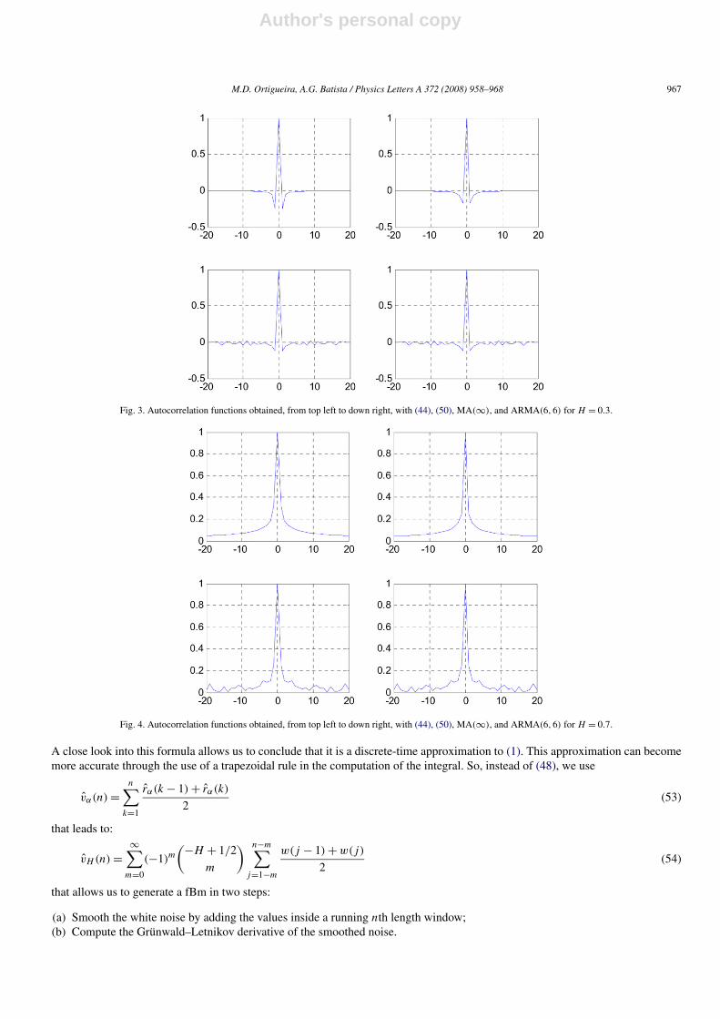
To have an idea of the difference in substituting the derivative for the difference, we generate 5000 points of fractional noise by com-puting the convolution of a truncated impulse response obtained from (49) with white Gaussian noise. The corresponding estimatedautocorrelation function is represented in the first picture in the second line. We present also the result obtained with the abovereferred ARMA model in the second picture of the second line. In the top pictures of each figure we present the autocorrelationfunctions obtained with (44) and (51). We used H = 0.3 in Fig. 3 and H = 0.7 in Fig. 4.

As expected, the estimated autocorrelations, although similar to the second in the first lines, are slightly different from the first.We should remark that we did not find any meaningful difference between the autocorrelations in the second line. This means thatthe ARMA model performs like the long MA system.

The formulation we proposed here is more general in the sense of giving the possibility of using other derivatives, specially theGrünwald–Letnikov like central derivatives [10,11]. Combining Eqs. (48) and (49) and permuting the two summations we obtainthe following approximation of fBm:

(52)v̂H (n) =∞∑

m=0

(−1)m(−H + 1/2

m

) n−m∑j=1−m

w(j).



Fig. 3. Autocorrelation functions obtained, from top left to down right, with (44), (50), MA(∞), and ARMA(6,6) for H = 0.3.

Fig. 4. Autocorrelation functions obtained, from top left to down right, with (44), (50), MA(∞), and ARMA(6,6) for H = 0.7.

A close look into this formula allows us to conclude that it is a discrete-time approximation to (1). This approximation can becomemore accurate through the use of a trapezoidal rule in the computation of the integral. So, instead of (48), we use

(53)v̂α(n) =n∑

k=1

r̂α(k − 1) + r̂α(k)

2

that leads to:

(54)v̂H (n) =∞∑

m=0

(−1)m(−H + 1/2

m

) n−m∑j=1−m

w(j − 1) + w(j)

2

that allows us to generate a fBm in two steps:

(a) Smooth the white noise by adding the values inside a running nth length window;(b) Compute the Grünwald–Letnikov derivative of the smoothed noise.



6. Conclusions

In this Letter, we deduced a new relation between the fractional Brownian motion and the fractional derivatives of white noise.We made a brief approach into the definitions of fractional derivatives suitable for stationary stochastic processes. We consideredtwo sets of fractional derivatives: (a) the forward and backward and (b) the central derivatives. For both sets we presented twoformulations: (a) Grünwald–Letnikov and similar, and (b) integral. We showed that for these derivatives the corresponding auto-correlation functions have the same representations. The results we obtained were used to define a fractional noise and, from it, thefractional Brownian motion. We presented its properties. This gives rise to new ways of simulating the fractional Brownian motion,mainly with the use of the Grünwald–Letnikov and similar derivatives. We performed a brief study of this subject where we madea test to an ARMA approximation to the fractional derivative for generating a fractional noise.

References

[1] B.B. Mandelbrot, J.W. Van Ness, SIAM Rev. 10 (4) (1968) 422.[2] B.B. Mandelbrot, The Fractal Geometry of Nature, W.H. Freeman and Company, New York, 1983.[3] M.S. Keshner, Proc. IEEE 70 (1982) 212.[4] I.S. Reed, P.C. Lee, T.K. Truong, IEEE Trans. Inform. Theory 41 (5) (1995) 1439.[5] N.A. Kolmogorov, Wienersche Spiralen und einige andere interessante Kurven im Hilbertschen Raum, C. R. Acad. Sci. URSS 26 (2) (1940) 115.[6] M.D. Ortigueira, A.G. Batista, Nonlinear Dynam. 38 (2004) 295.[7] M.D. Ortigueira, A.G. Batista, On the fractional derivative of stationary stochastic processes, in: Proceedings of the Conference ECT2006, Special Session

Fractional Differential Equations: Theory and Applications, Las Palmas, Spain, September 2006.[8] M.D. Ortigueira, Fract. Calc. Appl. Signals Systems 10 (2006) 2505.[9] M.D. Ortigueira, F.V.C. Coito, Fract. Calc. Appl. Anal. 7 (4) (2004).

[10] M.D. Ortigueira, Fractional centred differences and derivatives, in: Proceedings of the 2nd IFAC Workshop on Fractional Differentiation and Its Applications,Porto, Portugal, July 2006.

[11] M.D. Ortigueira, Int. J. Math. Math. Sci. 2006 (2006), Article ID 48391.[12] I. Podlubny, Fractional Differential Equations, Academic Press, San Diego, 1999.[13] S.G. Samko, A.A. Kilbas, O.I. Marichev, Fractional Integrals and Derivatives – Theory and Applications, Gordon and Breach Science, Amsterdam, 1993.[14] M.D. Ortigueira, IEE Proc. Vision Image Signal Process. 1 (2000) 71.[15] A.H. Zemanian, Distribution Theory and Transform Analysis, Dover, New York, 1987.[16] G.E. Andrews, R. Askey, R. Roy, Special Functions, Cambridge Univ. Press, 1999.[17] J.F. Coeurjolly, J. Stat. Software 5 (2000) 1.[18] B.M. Vinagre, I. Podlubny, A. Hernandez, V. Feliu, Fract. Calc. Appl. Anal. 3 (3) (2000) 231.[19] J.A. Tenreiro Machado, Fract. Calc. Appl. Anal. J. 1 (2001) 47.[20] M.D. Ortigueira, A.J. Serralheiro, Fract. Calc. Appl. Signals Systems 10 (2006) 2582.[21] M.D. Ortigueira, A.J. Serralheiro, IET Control Theory Appl. 1 (1) (2007) 173.

On the relation between the fractional Brownian motion and the fractional derivatives

Documents

Transcript of On the relation between the fractional Brownian motion and the fractional derivatives