Rectified Brownian transport in corrugated channels: Fractional Brownianmotion and Lévy flightsBao-quan Ai, Zhi-gang Shao, and Wei-rong Zhong Citation: J. Chem. Phys. 137, 174101 (2012); doi: 10.1063/1.4764472 View online: http://dx.doi.org/10.1063/1.4764472 View Table of Contents: http://jcp.aip.org/resource/1/JCPSA6/v137/i17 Published by the American Institute of Physics. Additional information on J. Chem. Phys.Journal Homepage: http://jcp.aip.org/ Journal Information: http://jcp.aip.org/about/about_the_journal Top downloads: http://jcp.aip.org/features/most_downloaded Information for Authors: http://jcp.aip.org/authors

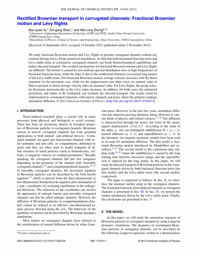
THE JOURNAL OF CHEMICAL PHYSICS 137, 174101 (2012)

Rectified Brownian transport in corrugated channels: Fractional Brownianmotion and Lévy flights

Bao-quan Ai,1 Zhi-gang Shao,1 and Wei-rong Zhong2,a)

1Laboratory of Quantum Information Technology, ICMP and SPTE, South China Normal University,510006 Guangzhou, China2Department of Physics, College of Science and Engineering, Jinan University, 510632 Guangzhou, China

(Received 14 September 2012; accepted 15 October 2012; published online 2 November 2012)

We study fractional Brownian motion and Lévy flights in periodic corrugated channels without anyexternal driving forces. From numerical simulations, we find that both fractional Gaussian noise andLévy-stable noise in asymmetric corrugated channels can break thermodynamical equilibrium andinduce directed transport. The rectified mechanisms for fractional Brownian motion and Lévy flightsare different. The former is caused by non-uniform spectral distribution (low or high frequencies) offractional Gaussian noise, while the latter is due to the nonthermal character (occasional long jumps)of the Lévy-stable noise. For fractional Brownian motion, average velocity increases with the Hurstexponent for the persistent case, while for the antipersistent case there exists an optimal value ofHurst exponent at which average velocity takes its maximal value. For Lévy flights, the group veloc-ity decreases monotonically as the Lévy index increases. In addition, for both cases, the optimizedperiodicity and radius at the bottleneck can facilitate the directed transport. Our results could beimplemented in constrained structures with narrow channels and pores where the particles undergoanomalous diffusion. © 2012 American Institute of Physics. [http://dx.doi.org/10.1063/1.4764472]

I. INTRODUCTION

Noise-induced transport plays a crucial role in manyprocesses from physical and biological to social systems.There has been an increasing interest in transport proper-ties of Brownian particles in corrugated channels. Brownianmotion in narrow corrugated channels has wide potentialapplications to both natural1 and artificial devices.2 Corru-gated channels are quasi-one-dimensional channels with ax-ial symmetry and unit cells, or compartments, delimited bypores and they are often used to model transport of di-lute mixtures of small particles (such as biomolecules, col-loids, or magnetic vortices) in confined geometries.2 Broadlyspeaking, the corrugated channels fall into two categoriesdepending on the geometry of the channel wall: Smoothlycorrugated channels3–9 and compartmentalized channels.10–12

In smoothly corrugated channels, the movement equationof Brownian particles can be described by the Fick-Jacobsequation3–9 which is derived from the three-dimensional ortwo-dimensional Smoluchowski equation after elimination ofy and z coordinates by assuming equilibrium in the orthogo-nal directions. The reduction of the coordinates can involvethe appearance of entropic barrier and smoothly corrugatedchannels can also be called entropic channels. However, thediffusion of Brownian particles in compartmentalized chan-nels cannot be reduced to an effective one-dimensional ki-netic process directed along the axis. The behaviors of thequantities of interest can be described by Brownian dynamicssimulations.

Most studies on corrugated channels have referred tothe consideration of normal diffusion driven by white Gaus-

a)E-mail: wrzhong@jnu.edu.cn.

sian noise. However, in the past few years, anomalous diffu-sion has attracted growing attention, being observed in vari-ous fields of physics and related sciences.13–26 The diffusionis characterized through the power law form of the mean-square displacement 〈x2(t)〉∝ tα . According to the value ofthe index μ, one can distinguish subdiffusion (0 < μ < 1),normal diffusion (μ = 1), and superdiffusion (μ > 1). Inthe literature, two popular stochastic models have been usedto account for anomalous diffusion. The first model is frac-tional Brownian motion introduced by Mandelbrot and co-authors.13–19 The second model is the continuous-time ran-dom walk,20–26 where the subdiffusion is caused by the longwaiting time between successive jumps and the superdiffu-sion is induced by the long jumps. In this paper, we willstudy the directed transport of Brownian particles in the corru-gated channels driven by both fractional Gaussian noise (thefirst model) and the Lévy-stable noise (the second model),respectively.

The paper is organized as follows. In Sec. II, we intro-duce the minimal ratchet setup in the corrugated channels.The fractional Gaussian noise-induced transport in corrugatedchannels is presented in Sec. III. In Sec. IV, we present theratchet mechanism driven by the Lévy-stable noise. Finally,the conclusions are presented in Sec. V.

II. THE MODEL

In this paper, we will study the anomalous transport ofBrownian particles in corrugated channels by using Langevindynamics simulations. The dynamics of overdamped Brow-nian particles in corrugated channels can be described bythe following Langevin equations written in a dimensionless

0021-9606/2012/137(17)/174101/7/$30.00 © 2012 American Institute of Physics137, 174101-1

174101-2 Ai, Shao, and Zhong J. Chem. Phys. 137, 174101 (2012)

(x) x

y

xbr2

Slanted side Steeper side

FIG. 1. Schematic diagram of a channel with periodicity L. The shape is described by the radius of the channel ω(x) = a[sin( 2πxL

) + �4 sin( 4πx

L)] + b.

form:

ηdx

dt=

√ηkBT ξx(t), (1)

ηdy

dt=

√ηkBT ξy(t), (2)

where x and y are the two-dimensional coordinates. ξ x, y(t) isthe noise, D = kBT

ηis noise intensity. η is the friction coef-

ficient of the particle, kB is the Boltzmann constant, and T isthe absolute temperature. The noise will be fractional Gaus-sian noise in Sec. III and Lévy-stable noise in Sec. IV.

The shape of the channel can be described by its radiusshown in Fig. 1

ω(x) = a

[sin

(2πx

L

)+ �

4sin

(4πx

L

)]+ b, (3)

where � is the asymmetry parameter of the channel shapeand a is the parameter that controls the slope of the channel.The radius rb at the bottleneck is determined by the parame-

ters a, b, and �, rb = b − a

√1 + �2

16 , when � = 4a

√b2 − a2,

rb = 0, and the channel is blocked.Though the movement equation of Brownian particles in

corrugated channels can be usually described by the Fick-Jacobs equation,3–9 the corresponding Fick-Jacobs equationfor anomalous diffusion is still not available. The study ofthese transport phenomena is in many respects equivalentto an investigation of geometrically constrained Browniandynamics.19 The behavior of the quantities of interest canbe corroborated by Brownian dynamic simulations performedby integration of the Langevin equation using the standardstochastic Euler algorithm. From Eqs. (1) and (2) and thestandard stochastic Euler algorithm, the single integrationsteps read

x(tn+1) = x(tn) + fx(D, δt, ξx(n)), (4)

y(tn+1) = y(tn) + fy(D, δt, ξy(n)), (5)

where n = 0, 1, 2. . . and fx, y is the noise term in the Eu-ler algorithm. Imposing reflecting boundary conditions in thetransverse direction (the channel wall) ensures the confine-ment of the dynamics within the channel, while periodicboundary conditions are enforced along the longitudinal di-rection. δt is time step ranging from 10−4 down to 10−5 andfor each run the output is independent of δt.

The key quantifier to characterize the directed transportof Brownian particles in sinusoidally corrugated channel isx-direction velocity which can be obtained from the numer-ical simulations based on Eqs. (4) and (5). Especially, in thesimulations, we use the average velocity for fractional Brown-ian transport in Sec. III and the group velocity for Lévy flightsin Sec. IV. In this paper, we mainly focus on anomalous diffu-sion in corrugated channels. Two typical anomalous diffusionmodels, fractional Brownian motion and Lévy flights are in-vestigated in Sec. III and Sec. IV, respectively.

III. FRACTIONAL BROWNIAN MOTION

In the last few years, there has been a growing interestin the study of the fractional Brownian motion. FractionalBrownian motion has wide applications in some complexsystems,27 such as monomer diffusion in a polymer chain,single file diffusion, translocation of the polymer passingthrough a pore, and diffusion of biopolymers in the crowdedenvironment.

Fractional Gaussian noise is a zero mean stationary ran-dom process with long memory effects.14–19 It is closely re-lated to the Fractional Brownian motion process,19 which isdefined as a Gaussian process with Hurst exponent 0 < H< 1 and

〈ξH (t)〉 = 0, (6)

〈ξH (t)ξH (s)〉 = 1

2[t2H + s2H − (t − s)2H ], (7)

for 0 < s ≤ t. The fractional Gaussian noise reduces to whiteGaussian noise at H = 1

2 . When H �= 12 , the autocorrelation

function in the long time limit will decay as

〈ξH (0)ξH (t)〉 ∝ 2H (2H − 1)t2H−2. (8)

From the above equation, we can easily find that the noisesare negatively correlated (antipersistent case) for 0 < H < 1

2

and positively correlated (persistent case) for 12 < H < 1.

When the fractional Gaussian noises apply to the systems(1) and (2), Eqs. (4) and (5) can be rewritten as

x(tn+1) = x(tn) +√

DδtH ξxH (n), (9)

y(tn+1) = y(tn) +√

DδtH ξy

H (n), (10)

174101-3 Ai, Shao, and Zhong J. Chem. Phys. 137, 174101 (2012)

where ξx,y

H (n) is fractional Gaussian random number. We usedthe method described in Refs. 28 and 29 for simulating frac-tional Gaussian random number.

From Eqs. (9) and (10), the x-direction average velocitycan be obtained from the following formula:

V = 1

Nlimt→∞

N∑i=1

xi(t) − xi(t0)

t − t0, (11)

where t0 and t are the initial and the end time for the simu-lations, respectively. N is the number of the realizations. Thestochastic averages reported above were obtained as ensembleaverages over 3 × 105 trajectories with random initial con-ditions. The transient effects were estimated and subtracted.From Eqs. (9)–(11), we can numerically obtain the averagevelocity of the Brownian particles.

The frequency spectrum of the external drive is very im-portant to determine direction of motion of the Brownianparticles in periodic potentials or structures. For stationarystochastic processes, the spectral density is computed as fol-lows for frequencies −π ≤ f ≤ π . The spectral density offractional Gaussian noise can be given by Refs. 29 and 30:

P (f ) = 2 sin(πH )(2H + 1)(1 − cos(f )

× [|f |−2H−1 + B(f,H )] (12)

with

B(f,H ) =∞∑

j=1

{(2πj + f )−2H−1 + (2πj − f )−2H−1}.

(13)From Eqs. (12) and (13), we can numerically evaluate thespectral density by truncating method29, 30 for different val-ues of H. The spectral density distributions for different casesare shown in Fig. 2. We can find that the distributions of thefrequency are different for the three cases. For white Gaus-sian noise (H = 0.5), the spectral density is uniform. For theantipersistent case (H = 0.3), the high frequency componentis larger in the spectral density. However, the low-frequencycomponent is larger than the high-frequency part in the spec-tral density for the persistent case (H = 0.7). In order to fa-cilitate the analysis of the driving mechanisms, the persistentfractional Gaussian noise can be artificially divided into twocomponents: white Gaussian noise and the low-frequency ac

0.2 0.4 0.6 0.8 10

0.5

1

1.5

2

2.5

frequency/π

Sp

ectr

al d

ensi

ty

H=0.3H=0.5H=0.7

FIG. 2. The spectral density P(f) for H = 0.3, H = 0.5, and H = 0.7.

drive. Similarly, the antipersistent fractional Gaussian noisein frequency domain is equivalent to a compound of whiteGaussian noise and the high-frequency drive.

Now, we will study the directed transport mechanism forfractional Brownian motion. For simplicity, we consider thecase of � = −1. The only resource force is the fractionalGaussian noise. When H = 1

2 , the fractional Gaussian noisereduces to the white Gaussian noise, the system is in thermalequilibrium and no net current occurs. However, for H �= 1

2 ,the net current will occur. First, the particles are assume tostay in the valley of the channel (shown in Fig. 1) awaitingthe drive to be catapulted out. The particles will be thrownout to the left and the right with the equal probabilities. ForH > 1

2 , the fractional Gaussian noise can be treated as a low-frequency ac driving force and the Brownian particles getenough time to cross the both side from the valley of the chan-nel before the driving force changes its sign. In this case, it iseasier for the particles moving toward the slanted side than to-ward the steeper side, so the current is negative (shown in Fig.3(b)). For H < 1

2 , the fractional Gaussian noise can be treatedas the high-frequency ac driving force. Due to the higher fre-quency the Brownian particles do not get enough time to crossthe slanted side (the left side) which is at a larger distancefrom the valley of the channel. Therefore, before the forcechanges its direction, more particles cross the barrier fromthe valley to the steeper side (the right side), resulting in apositive current (shown in Fig. 3(a)).

From Fig. 3(a), we can find that for H < 12 there exists

a value of the Hurst exponent at which the average velocitytakes its maximal value. Obviously, when H → 0, the noiseterm in Eqs. (1) and (2) disappears, the average velocity goesto zero. When H → 1

2 , the noise reduces to the Gaussiannoise, and the average velocity tends to zero, also. For per-sistent case (H > 1

2 ) shown in Fig. 3(b), the absolute value ofthe average velocity increases with the Hurst exponent.

Figure 4 shows the dependence of the average velocityV on the asymmetric parameter � for the persistent case(H = 0.3). It is found that the average velocity is positivefor � < 0, zero at � = 0, and negative for � > 0. Fur-thermore, the average velocity tends to zero for large val-ues of �. When � ≥ 4

a

√b2 − a2, rb ≤ 0, and the channel

is blocked, then the particle cannot pass from one cell ofthe channel to the other cell. The curve for the antipersistentcase is similar to the curve in Fig. 4, but the sign of the av-erage velocity is opposite. Therefore, we can have the cur-rent reversal by changing the sign of �, the asymmetry ofchannel.

Figure 5 describes the average velocity V as a function ofthe periodicity L for both persistent and antipersistent cases.It is found that there exists an optimal value of L at whichthe average velocity takes its maximal value for both cases.When L → 0, the cell of the channel disappears, the effectof the asymmetric shape also disappears, then the average ve-locity goes to zero. When L → ∞ so that the length of eachcell of the channel is too long, the effect of the asymmetricshape of the channel also disappears and the average velocitytends to zero, also. It should be pointed out that the optimumL maximizing the velocity should depend on the parametersof the system, such as a, b, �, and D. Moreover, if we change

174101-4 Ai, Shao, and Zhong J. Chem. Phys. 137, 174101 (2012)

FIG. 3. Average velocity V as a function of the Hurst exponent H. (a) H < 0.5, (b) H > 0.5. The other parameters are a = 0.5, b = 0.7, D = 0.5, � = −1.0,and L = 1.0.

FIG. 4. Average velocity V as a function of the asymmetric parameter �

at H = 0.3. The other parameters are a = 0.5, b = 0.7, D = 0.5, andL = 1.0.

FIG. 5. Average velocity V as a function of the periodicity L for differ-ent values of H. The other parameters are a = 0.5, b = 0.7, D = 0.5, and� = −1.0.

the sign of � which determines the asymmetry of the channel,so the velocity has to change only the sign, too.

Figure 6 shows the average velocity V as a function ofthe radius rb at the bottleneck for both the persistent and an-tipersistent cases. When rb → 0, the channel is blocked andthe average velocity tends to zero. When rb → ∞, the effectof the asymmetric shape of the channel disappears. Therefore,the average velocity goes to zero, also. So there exists an op-timized value of rb at which the particles have the maximalaverage velocity.

IV. LÉVY FLIGHTS

Recently, description of physical models in terms of Lévyflights becomes more and more popular. They are actually ob-served in various real systems and are used to model a varietyof processes,31 such as bulk mediated surface diffusion, trans-port in micelle systems or heterogeneous rocks, exciton andcharge transport in polymers, two-dimensional rotating flow,and many others.

FIG. 6. Average velocity V as a function of rb for different values of H. Theother parameters are a = 0.5, D = 0.5, � = −1.0, and L = 1.0.

174101-5 Ai, Shao, and Zhong J. Chem. Phys. 137, 174101 (2012)

The symmetric Lévy-stable noise ζ α(t) has independentincrements distributed according to the stable density with theindex α. The time integral of the Lévy noise over an increment�t

Lα,σ (�t) =∫ t+�t

t

ζα(t ′)dt ′ (14)

is an α-stable process with stationary independent incrementsand its characteristic function is defined as20, 32, 33

PL(k,�t) = exp(−σ |k|α�t), (15)

where σ is the intensity of the Lévy noise and k is thewavenumber. The parameter α ∈ (0, 2] denotes the stabilityindex, yielding the asymptotic long tail power law for the ζ -distribution with |ζ |−1 − α type. For the special case α = 2.0,the Lévy noise reduces to the Gaussian noise.

When the white symmetric Lévy-stable noises apply tothe systems (1) and (2), Eqs. (4) and (5) can be rewritten as

x(tn+1) = x(tn) + (D�t)1α ζ x

α (n), (16)

y(tn+1) = y(tn) + (D�t)1α ζ y

α (n), (17)

where ζx,yα (n) is a random number possessing Lévy stable

distribution. In numerical simulations, the corresponding ran-dom numbers are taken from20, 32, 33

ζα(n) = sin(αU )

(cos U )1/α

[cos([1 − α]U )

W

] 1−αα

, (18)

where W is an independent random variable distributed ac-cording to the exponential distribution with unit mean andU is a random number uniformly distributed on the interval(−π /2, π /2).

For the noise with distribution of a Lévy-stable law, themean of the noise and the overall displacement do not exist.As a consequence, the average velocity, which is based onthe ordinary central limit theorem, is no longer valid. There-fore, we use the group velocity proposed by Dybiec and co-workers24 to describe the transport of the particles driven bythe Lévy-stable noises.

Median line is a very useful tool for investigation of theoverall motion of the probability density of finding a particlein the vicinity of x.21 A median line for a stochastic processx(t) is a function of q0.5(t) given by the relationship Pr(x(t)≤ q0.5(t)) = 0.5. Therefore, one can define the group velocityof the particle packet,

Vg = limt→∞

q0.5(t)

t(19)

and this definition is valid even for the case of lacking averagecurrent. From Eqs. (16), (17), and (19), we can calculate thegroup velocity of the Brownian particles. For simplicity, weonly consider the case of 1 < α ≤ 2 in our study.

In this minimal ratchet model, the only drive is the Lévy-stable noise. We first compare the trajectories of the Lévyflights with normal Brownian motion shown in Fig. 7. By con-trast, the Lévy walker occasionally takes long jumps to newterritory. The jumps become longer for smaller values of theLévy index. The long jumps in corrugated channels can breakthermodynamical equilibrium and induce directed transport.

FIG. 7. Comparison of the trajectories of Brownian motion (α = 2.0) andthe Lévy flights (α = 1.1, 1.5).

Figure 8 shows the group velocity Vg as a function ofthe asymmetric parameter � for α = 1.1. We can find thatthe group velocity is positive for � > 0, zero at � = 0, andnegative for � < 0. The group velocity tends to zero as theasymmetric parameter � increases to the large values. When� is very large, the radius rb at the bottleneck tends to zeroand the particles cannot jump from one cell of the channel tothe next cell, thus the group velocity goes to zero.

Similar to the case of the fractional Brownian transport,we also choose � = −1 for giving the physical interpretationof the rectifying mechanics in Lévy flights. First, the particlesstay in the valley of the channel (shown in Fig. 1) awaitinglarge noise pulse to be catapulted out. The particles will bethrown out to the left and the right with the equal probabili-ties. In this case, the distance from the valley to the bottleneckis shorter from the right side (the steeper side) than that fromthe left side (the slanted side). Consequently, most of the par-ticles are thrown out from the right side, resulting in positivetransport. This gives rise to the overall preferred motion to theright.

FIG. 8. Group velocity Vg as a function of the asymmetric parameter �. Theother parameters are α = 1.1, a = 0.5, b = 0.7, D = 0.5, and L = 1.

174101-6 Ai, Shao, and Zhong J. Chem. Phys. 137, 174101 (2012)

FIG. 9. Group velocity Vg as a function of the Lévy index α for differentvalues of �. The other parameters are a = 0.5, b = 0.7, D = 0.5, and L = 1.

The dependence of the group velocity on the Lévy indexα is shown in Fig. 9. We can see that the absolute value of Vg

increases as the Lévy index α decreases. When the index α

decreases, the Lévy flights become longer and the outliers inthe Lévy noise are larger (see Fig. 7), thus the larger current isobtained. When α → 2.0, the noise reduces to white Gaussiannoise, the system is in thermal equilibrium and no net currentoccurs.

Similar to the fractional Brownian transport in Sec. III,we also analyzed the effects of the periodicity L and the ra-dius rb at the bottleneck on the group velocity in Lévy flights.There exist optimal values of L and rb at which the groupvelocity takes its maximal value. Therefore, in this case, theoptimized periodicity and radius at the bottleneck can also fa-cilitate the directed transport.

V. CONCLUDING REMARKS

In this paper, we studied the directed transport of theoverdamped Brownian particles in periodic corrugated chan-nels driven by fractional Gaussian noise and Lévy-stablenoise. We find that both fractional Gaussian noise and Lévy-stable noise can induce the directed transport in periodic cor-rugated channels without any external forces. The former iscaused by non-uniform spectral distribution of the fractionalGaussian noise and the latter is caused by the nonthermalcharacter of the Lévy-stable noise.

For fractional Brownian motion, the fractional Gaussiannoise can be treated as the low-frequency ac drive for per-sistent case and high-frequency ac drive for antipersistentcase. Due to the special spectral distribution, the fractionalGaussian noise can break the thermodynamical equilibriumand induce the directed transport. The sign of the net currentis determined by the spectral properties of the noise and theasymmetry of the channels. Under the same conditions, thesign of the current driven by the persistent noise is opposite tothat driven by the antipersistent noise. For the persistent case,the average velocity increases with the Hurst exponent, whilefor the antipersistent case there exists the optimal value ofHurst exponent at which the average velocity takes its extreme

value. For Lévy flights, the Lévy-stable noise contains thelarger outliers which can break the thermodynamical equilib-rium and induce the directed transport. In this case the groupvelocity is used to describe the direction transport and the signof the net current is only determined by the asymmetry of thechannels. The group velocity decreases monotonically as theLévy index increases. In addition, for both cases, there ex-ist optimal values of L and rb at which the velocity reachesits extremal value. Therefore, the optimized periodicity L andradius rb at the bottleneck can facilitate the directed transport.

ACKNOWLEDGMENTS

This work was supported in part by the NationalNatural Science Foundation of China (Grant Nos.11004082, 11175067, and 11105054), the Natural Sci-ence Foundation of Guangdong Province, China (GrantNos. 10451063201005249 and S201101000332), and theFundamental Research Funds for the Central Universities,JNU (Grant No. 21611437).

1B. Hille, Ion Channels of Excitable Membranes (Sinauer, Sunderland,2001); J. Karger and D. M. Ruthven, Diffusion in Zeolites and Other Mi-croporous Solids (Wiley, New York, 1992).

2P. Hanggi and F. Marchesoni, Rev. Mod. Phys. 81, 387 (2009).3P. S. Burada, P. Hanggi, F. Marchesoni, G. Schmid, and P. Talkner,ChemPhysChem 10, 45 (2009); D. Reguera and J. M. Rubi, Phys. Rev.E 64, 061106 (2001); D. Reguera, G. Schmid, P. S. Burada, J. M. Rubi, P.Reimann, and P. Hanggi, Phys. Rev. Lett. 96, 130603 (2006); P. S. Burada,G. Schmid, D. Reguera, J. M. Rubi, and P. Hanggi, Phys. Rev. E 75, 051111(2007); D. Reguera, A. Luque, P. S. Burada, G. Schmid, J. M. Rubi, and P.Hanggi, Phys. Rev. Lett. 108, 020604 (2012).

4R. Zwanzig, J. Phys. Chem. 96, 3926 (1992).5P. Kalinay and J. K. Percus, Phys. Rev. E 74, 041203 (2006); 72, 061203(2005); P. Kalinay, ibid. 84, 011118 (2011); P. Kalinay and J. K. Percus,ibid. 82, 031143 (2010).

6N. Laachi, M. Kenward, E. Yariv, and K. D. Dorfman, Europhys. Lett. 80,50009 (2007).

7R. Reichelt, S. Gunther, J. Wintterlin, W. Moritz, L. Aballe, and T. O.Mentes, J. Phys. Chem. 127, 134706 (2007).

8D. Mondal and D. S. Ray, Phys. Rev. E 82, 032103 (2010); D. Mondal,M. Das, and D. S. Ray, J. Chem. Phys. 132, 224102 (2010); 133, 204102(2010); M. Das, D. Mondal, and D. S. Ray, ibid. 136, 114104 (2012); D.Mondal and D. S. Ray, ibid. 135, 194111 (2011).

9B. Q. Ai and L. G. Liu, Phys. Rev. E 74, 051114 (2006); B. Q. Ai, ibid. 80,011113 (2009).

10F. Marchesoni and S. Savel’ev, Phys. Rev. E 80, 011120 (2009); F.Marchesoni, J. Chem. Phys. 132, 166101 (2010); M. Borromeo and F.Marchesoni, Chem. Phys. 375, 536 (2010); M. Borromeo, F. Marchesoni,and P. K. Ghosh, J. Chem. Phys. 134, 051101 (2011); P. K. Ghosh and F.Marchesoni, ibid. 136, 116101 (2012).

11Yu. A. Makhnovskii, A. M. Berezhkovskii, and V. Yu. Zitserman, J. Chem.Phys. 131, 104705 (2009); A. M. Berezhkovskii, L. Dagdug, Yu. A.Makhnovskii, and V. Yu. Zitserman, ibid. 132, 221104 (2010).

12P. Hanggi, F. Marchesoni, S. Savel’ev, and G. Schmid, Phys. Rev. E 82,041121 (2010); P. K. Ghosh, P. Hanggi, F. Marchesoni, F. Nori, and G.Schmid, ibid. 86, 021112 (2012).

13B. B. Mandelbrot and J. W. Van Ness, SIAM Rev. 10, 422 (1968).14I. Calvo and R. Sanchez, J. Phys. A: Math. Theor. 41, 282002 (2008);

M. Bologna, F. Vanni, A. Krokhin, and P. Grigolini, Phys. Rev. E 82,020102(R) (2010); L. Zunino, D. G. Perez, M. T. Martin, M. Garavaglia,A. Plastino, and O. A. Rosso, Phys. Lett. A 372, 4768 (2008).

15T. A. Øigard, A. Hanssen, and L. L. Scharf, Phys. Rev. E 74, 031114(2006); W. Deng and E. Barkai, ibid. 79, 011112 (2009); J. H. Jeon andR. Metzler, ibid. 81, 021103 (2010).

16R. Garcia-Garcia, A. Rosso, and G. Schehr, Phys. Rev. E 81, 010102(R)(2010); N. Kumar, U. Harbola, and K. Lindenberg, ibid. 82, 021101 (2010).

17M. Magdziarz, A. Weron, K. Burnecki, and J. Klafter, Phys. Rev. Lett. 103,180602 (2009); I. Eliazar and J. Klafter, Phys. Rev. E 79, 021115 (2009).

174101-7 Ai, Shao, and Zhong J. Chem. Phys. 137, 174101 (2012)

18O. Y. Sliusarenko, V. Y. Gonchar, A. V. Chechkin, I. M. Sokolov, and R.Metzler, Phys. Rev. E 81, 041119 (2010).

19S. C. Kou and X. S. Xie, Phys. Rev. Lett. 93, 180603 (2004).20R. Metzler and J. Klafter, Phys. Rep. 339, 1 (2000); A. V. Chechkin, O. Y.

Sliusarenko, R. Metzler, and J. Klafter, Phys. Rev. E 75, 041101 (2007).21M. Magdziarz and A. Weron, Phys. Rev. E 75, 056702 (2007); M.

Magdziarz, A. Weron, and K. Weron, ibid. 75, 016708 (2007).22D. Kleinhans and R. Friedrich, Phys. Rev. E 76, 061102 (2007); H. C.

Fogedby, ibid. 50, 1657 (1994).23I. Goychuk, E. Heinsalu, M. Patriarca, G. Schmid, and P. Hänggi, Phys.

Rev. E 73, 020101(R) (2006); E. Heinsalu, M. Patriarca, I. Goychuk, G.Schmid, and P. Hänggi, ibid. 73, 046133 (2006).

24B. Dybiec, E. Gudowska-Nowak, and I. M. Sokolov, Phys. Rev. E78, 011117 (2008); B. Dybiec, ibid. 78, 061120 (2008); 80, 041111(2009).

25D. Del-Castillo-Negrete, V. Yu. Gonchar, and A. V. Chechkin, Physica A387, 6693 (2008).

26J. Rosa and M. W. Beims, Physica A 386, 54 (2007).27G. Guigas and M. Weiss, Biophys. J. 94, 90 (2008); J. Szymanski and M.

Weiss, Phys. Rev. Lett. 103, 038102 (2009); L. Lizana and T. Ambjornsson,ibid. 100, 200601 (2008); A. Zoia, A. Rosso, and S. N. Majumdar, ibid.102, 120602 (2009).

28A. V. Checkin and V. Y. Gonchar, Chaos, Solitons Fractals 12, 391 (2001);B. S. Lowen, Methodol. Comput. Appl. Probab. 1(4), 445 (1999).

29T. Dieker, “Simulation of fractional Brownian motion,” Master’s thesis(University of Twente, 2004).

30V. Paxson, Comput. Commun. Rev. 27, 5 (1997).31O. V. Bychuk and B. O’Shaughnessy, Phys. Rev. Lett. 74, 1795 (1995); M.

A. Lomholt, T. Ambjornsson, and R. Metzler, ibid. 95, 260603 (2005); T.H. Solomon, E. R. Weeks, and H. L. Swinney, ibid. 71, 3975 (1993).

32A. Talnoi and F. Marchesoni, Phys. Rev. Lett. 96, 020601 (2006).33A. Janick and A. Weron, Stat. Sci. 9, 109 (1994); R. Weron, Stat. Probab.

Lett. 28, 165 (1996); J. M. Chambers, C. Mallows, and B. W. Stuck, J. Am.Stat. Assoc. 71, 340 (1976).