Rod-like Brownian Particles in Shear Flow
115
Rod-like Brownian Particles in Shear Flow Jan K.G. Dhont, W.J. Briels WILEY-VCH Verlag Berlin GmbH December 22, 2004
-
Upload
khangminh22 -
Category
Documents
-
view
0 -
download
0
Transcript of Rod-like Brownian Particles in Shear Flow
Rod-like Brownian Particles inShear Flow
Jan K.G. Dhont, W.J. Briels
WILEY-VCH Verlag Berlin GmbHDecember 22, 2004


Preface
This chapter is a self-contained treatment of various aspects concerning suspensions of uni-axial rod-like colloidal particles in flow. First of all, friction coefficients of rods in an otherwiseunbounded fluid will be calculated and the motion of a single rod in flow will be discussed,both for a non-Brownian and a Brownian rod. The generalized diffusion equation for inter-acting rods, the so-called N-particle Smoluchowski equation is then discussed, on the basisof which the Doi-Edwards equation of motion for the orientational order parameter tensor isderived. This microscopic derivation reveals the approximations that are involved in the Doi-Edwards theory. One of the approximations involves the neglect of dynamical correlations.Computer simulations indicate that such correlations might be important. On the basis ofthe Doi-Edwards equation (supplemented with an appropriate closure relation) together withexperimental results, the phase behaviour of rods in simpleshear flow is addressed. A mi-croscopic expression for the stress tensor for suspensionsof rigid colloidal particles is thenderived, and subsequently expressed in terms of the orientational order parameter tensor. Theviscoelastic response of suspensions of stiff rods is discussed, and theory is compared withexperiments and simulations. In the last section, current research interests will be brieflydiscussed, including banding transitions, the non-equilibrium phase diagram under flow con-ditions and phase separation kinetics.
6
Julich
0.1 Introduction
Flow affects microstructural order of colloidal systems intwo respects : center-to-center cor-relations are affected by flow and flow can induce changes in orientational order. For sphericalcolloids, flow-induced changes of macroscopic properties find their origin entirely in shear-induced changes of center-to-center correlations. For non-spherical colloidal particles, thereis the additional effect that flow tends to align single colloidal particles due to the torques thatthe flowing solvent exerts on their cores. For very elongatedcolloidal cores, single particlealignment is dominant over shear-induced changes of center-to-center correlations. For suchsystems, equations for one-particle orientational distribution functions, with the neglect offlow-induced distortions of center-to-center correlations, are sufficient to predict their macro-scopic behaviour under flow. For spherical colloidal particles, however, one-particle distribu-tion functions are not affected by flow, so that theory for spheres should be based on equationsfor correlation functions.
This chapter deals with stiff, uni-axial colloidal rods with a very large aspect ratio in shearflow. It will be assumed throughout the chapter that the center-to-center correlation function isnot affected by flow, and is thus equal to the corresponding correlation function in equilibrium,in the absence of flow. In addition, the singlet function of rods surrounding a given rod is takenequal to the singlet function of that given rod at the same instant of time. As will be discussed,these two simplifications are equivalent to the neglect of dynamical correlations. There areindications from computer simulations, however, that dynamical correlations might play arole.
Examples of flow-affected macroscopic phenomena which willbe discussed in the presentchapter are the shear-induced shift of the isotropic-nematic phase transition and the shear-ratedependent viscoelastic response. The effect of shear flow onmicrostructural order, which is atthe origin of shear-induced macroscopic phenomena, will beconsidered in detail. In addition,shear flow induces phenomena which do not occur in the absenceof flow, such as patternformation (or more specific, shear banding) and dynamical states under stationary appliedflow. These will be addressed only briefly at the end of this chapter.
The aim of this chapter is to set up, in a self contained fashion, a microscopic theory ofthe behaviour of rods in flow. Some of the results presented here are on a text book level,some are re-derivations of well-known equations and some are at the edge of current researchinterests. Much of the introductory material on colloids isalso discussed by Doi and Edwards(1986), Russel, Saville, and Schowalter (1991) and Dhont (1996).
First of all, the so-calledvelocity gradient tensorwill be defined in section 2. This tensordescribes the type of flow that is applied. Two types of flow areof particular importance: simple shear flow and elongational (or, extensional) flow. Simple shear flow is a velocityprofile where the gradient in the fluid flow velocity is constant, whereas for elongational flowthe sample is compressed in one direction and elongated in the other direction. Such flowscan be either stationary or oscillatory.
Colloidal rods tend to align in a flow field due to the interaction of the solvent with thesurface of the core of the rods. As a first step to understand how orientational order is affected

0.1 Introduction 7
by flow, the force and torque of the solvent on a single rod in anotherwise unbounded fluidmust be calculated. Since the linear dimensions of the rods is much larger than the size ofsolvent molecules, the solvent can be described on the basisof hydrodynamics. The rod istreated as a macroscopic object as far as its interactions with solvent molecules is concerned.The basic knowledge of hydrodynamics relevant for colloidsis developed in section 3. Themain result here is that inertial effects can be neglected ona time scale that is relevant forcolloids, leading to the so-calledcreeping flow equationsfor the solvent flow velocity. Theseare linear equations of motion for which the Greens function, known asthe Oseen tensor, isderived in section 3. Friction of rods in a flowing solvent is then treated on basis of thesebasic hydrodynamic equations in section 4. Friction coefficients can be calculated exactlyfor ellipsoidal rods of arbitrary aspect ratio, which involves an exact solution of the creepingflow equations, Happel and Brenner (1983). Alternatively, friction coefficients are derived insection 4 on the basis of the bead model for a rod, by analyzingforces that act on beads.
Once the hydrodynamic friction coefficients are known, orbits of the orientation of a non-Brownian rod in a flow field can be analyzed. These so-calledJeffery orbitsare discussed insection 5. Here, interactions between rods are not incorporated, that is, the orbits of a singlerod in an otherwise unbounded fluid are considered.
Brownian motion in the absence of flow is then analyzed in section 6 on the basis of New-ton’s equation of motion. This equation of motion includes arandom force which describesforces originating from collisions of solvent molecules with the surface of the colloidal par-ticle. Such equations of motion containing a fluctuating term are referred to asLangevinequations. Specifying certain statistical properties of the random force allows to distinguishbetween several important time scales and the calculation of the mean squared displacement.Again, this analysis is performed for a single rod in an otherwise unbounded solvent.
For the description of Brownian motion and diffusion of rodsat higher rod concentration,where interactions between rods are important, it is more convenient to employ equations ofmotion for probability density functions. The fundamentalequation of motion of this sort,the so-calledSmoluchowski equationis derived in section 7. In the same section it is shownthat the diffusive properties as obtained in section 6 on thebasis of the Langevin equation arereproduced by the Smoluchowski equation.
At higher concentrations and when a flow field is applied, the orientational order can bequantified by means of theorientational order parameter tensorS. This tensor is introducedin section 8. It is shown that the largest eigenvalue of this tensor is a measure for the degreeof orientational order and that the corresponding eigenvector defines the preferred orientationof the rods.
Orientational order for very dilute rod-suspensions underflow are discussed in section 9.Interactions between rods are neglected here. Solutions ofthe Smoluchowski equation areshown to be in accordance with computer simulations.
Orientational order and phase behaviour of concentrated suspensions in flow is analyzedby means of an equation of motion for the order parameter tensor S, which is known astheDoi-Edwards equation. In section 10 this equation of motion is derived from the Smolu-chowski equation. This derivation is a microscopic basis ofthe Doi-Edwards equation, whichreveals the approximations that are implicit in the Doi-Edwards equation. To obtain a closedequation of motion for the second order tensorS, a closure relation must be used for a fourthorder tensor. There are a number of propositions for such a closure relation. A simple closure
8
relation will be discussed in section 10, which is shown to beaccurate to within about10 %.This particular closure relation, however, can not describe non-stationary states under station-ary flow conditions like tumbling and wagging. To describe such states, the Smoluchowskiequation itself should be solved numerically. This will notbe discussed in the present chapter.
The isotropic-nematic phase transition is discussed in section 11, both without and withsimple shear flow. The bifurcation diagram is introduced andthe paranematic-to-nematic andnematic-to-paranematic spinodals in the shear-rate versus concentration plane are calculated.The prediction of the shear-rate dependent location of binodals is much more complicated,and requires equations of motion for the orientational order parameter tensorand the flowfield velocity, which should accurately account for strong inhomogeneities in concentration,orientational order parameter and shear rate. Such equations of motion will not be derived inthis chapter, but only briefly discussed in the last section on current research.
In the derivation of the Doi-Edwards equation of motion fromthe Smoluchowski equa-tion, dynamical correlations are neglected. Computer simulations indicate, however, that suchcorrelations are important for the description of diffusion. The discrepancy between the an-alytically obtained effective collective diffusion coefficients within the Doi-Edwards theoryand that found in computer simulations is discussed in section 12.
A microscopic derivation of the stress tensor in terms of theconcentration and the orien-tational order parameter tensor is given in section 13. Within certain approximations, a verysimilar expression as in the Doi-Edwards-Kuzuu theory is obtained. On the basis of this ex-pression for the stress tensor, (non-linear) viscoelasticelastic response of rod suspensions isdiscussed in section 14. Analytical and numerical predictions are compared to experimentsand computer simulations. A surprising finding is that the zero-shear, zero-frequency shearviscosity is a linear function of the concentration up to very high concentrations, in accordancewith computer simulations. Comparison with experiments indicates a sensitive dependence ofthe viscoelastic behaviour on the flexiblity of the core of the rods. So far, no theory on thedynamics and viscoelastic response is available that incorporates flexibility.
Section 15 is a (certainly biased) overview of the current research interests in the field ofrod suspensions under shear flow. The possible non-equilibrium phase diagram is addressed,together with banding transitions, non-stationary statesand kinetics of phase separation andband formation.
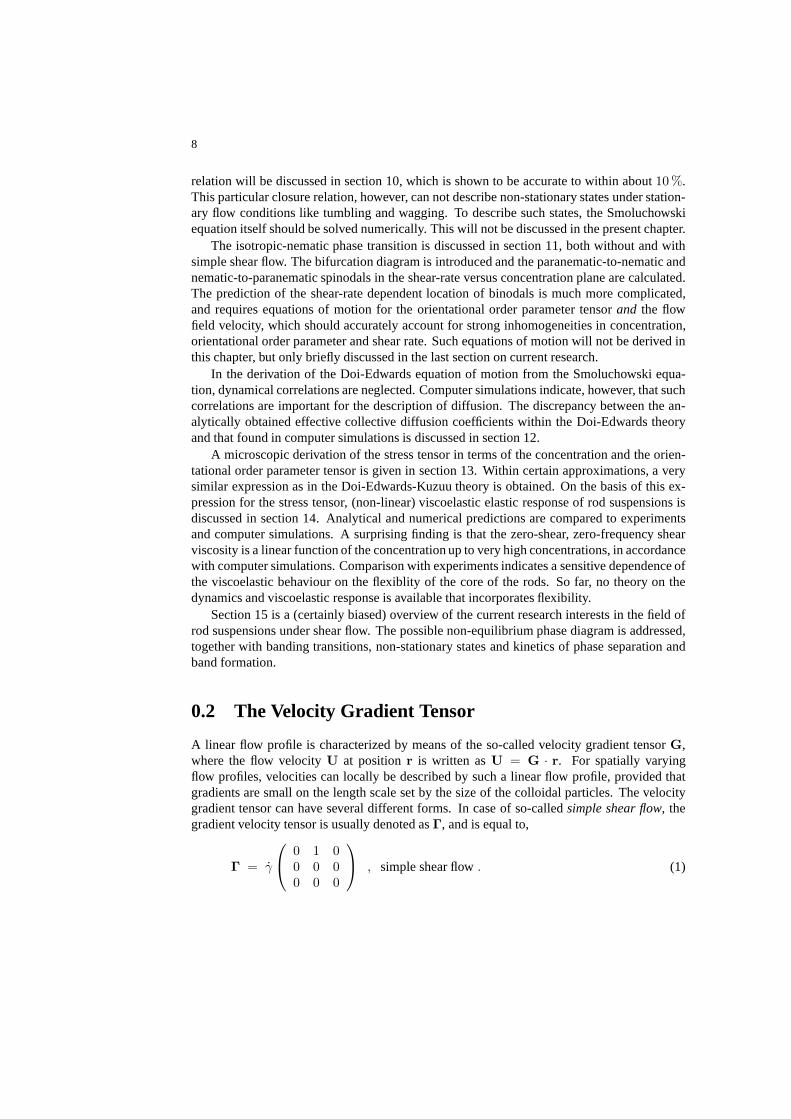
0.2 The Velocity Gradient Tensor
A linear flow profile is characterized by means of the so-called velocity gradient tensorG,where the flow velocityU at positionr is written asU = G · r. For spatially varyingflow profiles, velocities can locally be described by such a linear flow profile, provided thatgradients are small on the length scale set by the size of the colloidal particles. The velocitygradient tensor can have several different forms. In case ofso-calledsimple shear flow, thegradient velocity tensor is usually denoted asΓ, and is equal to,
Γ = γ
0 1 00 0 00 0 0
, simple shear flow. (1)

0.2 The Velocity Gradient Tensor 9
v = g L·
L
x
y
(a)
simple shear flow
(b)
extensional flow
(c)
rotational flow
extension
compression
v = g L·
v = g L·
L
x
y
(a)
simple shear flow
(b)
extensional flow
(b)
extensional flow
(b)
extensional flow
(c)
rotational flow
(c)
rotational flow
extension
compression
Figure 1: (a) Simple shear flow, whereL is the gapwidth. (b) Depicts elongational flow, sometimesalso referred to as extensional flow (where the elongationaland compression axes are indicated), and (c)depicts rotational flow. Arrows indicate the flow direction.
The corresponding flow profile is a flow in thex-direction, with its gradient in they-direction,as sketched in fig.1a. Thez-direction is commonly referred to as the vorticity direction. Thestrength of the flow is characterized by theshear rateγ, which equals the spatial gradient∂Ux/∂y of the flow velocityUx in thex-direction. For so-calledelongational or extensionalflow, where the velocity gradient tensor is denoted asE, we have,
E = γ
0 1 01 0 00 0 0
, elongational flow, (2)
which flow is sketched in fig.1b. In such an elongational flow, deformable objects tend toelongate along the so-called extensional axis, and suppressed along the compressional axis.These two directions are indicated in fig.1b. Whenever it is not specified whether simple shearflow or elongational flow is considered, the velocity gradient tensor will be denoted asG.
We will encounter the symmetric partE = 12
[
G + GT]
of the velocity gradient tensor,where the superscript “T ” stands for the transpose of the corresponding tensor. For elonga-tional flow, the velocity gradient tensor is already symmetric : this is why we denoted thevelocity gradient tensor for elongational flow by anE in eq.(2). For simple shear flow wehave,
E = 12γ
0 1 01 0 00 0 0
, simple shear flow. (3)
We will sometimes also encounter the anti-symmetric partΩ = 12
[
G − GT]
of the velocitygradient tensor. For elongational flow the anti-symmetric part is zero, while for simple shearflow we have,
Ω = 12γ
0 1 0−1 0 00 0 0
, simple shear flow. (4)

10
The flow velocities corresponding to flow with a velocity gradient tensor equal toE in eq.(3)or eq.(4) are sketched in fig.1b and c, respectively. The former case is an elongational flow,also referred to as extensional flow, while the second is purerotational flow. Note that,
Γ = E + Ω , (5)
so that simple shear flow can be decomposed into a linear combination of elongational androtational flow.
In laboratory experiments, the shear rate is either independent of time, or the shear ratecan be sinusoidally oscillating,
γ = time independent , stationary flow,
γ(t) = γ0 cosω t , oscillatory flow, (6)
whereω is the frequency of oscillation andγ0 is referred to as theshear-rate amplitude.Oscillatory experiments can be employed to probe the dynamics of a system of Brownianparticles.
0.3 Hydrodynamics
Consider a system containing large rod-like particles immersed in a fluid. There are threetypes of interactions to be distinguished in such a system : interactions of rods with rods,solvent molecules with solvent molecules and rods with solvent molecules. The latter twotypes of interactions can be described on the basis of phenomenological equations for fluidflow, provided that the linear dimensions of the rods are muchlarger than the size of solventmolecules. Such solutions of large molecules are referred to asBrownian or colloidal sys-tems. The large difference in relevant length scales between thesolvent and the assembly ofBrownian rods allows to describe the solvent on a phenomenological level, without losing themicroscopics for the assembly of Brownian particles. In such a phenomenological treatment,only macroscopic quantities of the fluid like its viscosity and mass density enter the equationsof interest. In the present section, friction coefficients of rods are calculated, which will beused later in this chapter in microscopic equations of motion for rod-like Brownian particles.
The mechanical state of the solvent is characterized by the local velocityu(r, t) at positionr at timet, the pressurep(r, t) and the mass densityρ(r, t). All these fields are averages oversmall volume elements that are located at the various positionsr. These volume elementsmust be so small that the state of the fluid hardly changes within the volume elements. At thesame time, the volume elements should contain many fluid molecules, to be able to properlydefine such averages. In particular we wish to define the thermodynamic state of volumeelements, which is possible when they contain a large amountof solvent molecules, and whenthey are in internal equilibrium, that is, when there islocal equilibrium. In this way thetemperature fieldT (r, t) may be defined. The temperature dependence of, for example, themass density is then described by thermodynamic relations.These thermodynamic relationsare an important ingredient in a general theory of hydrodynamics. For our purposes, however,the temperature and mass density may be considered constant. Temperature variations due toviscous dissipation in the solvent are assumed to be negligible. At constant temperature, theonly mechanism to change the mass density of the solvent is tovary the pressure. For fluids,
0.3 Hydrodynamics 11
however, exceedingly large pressures are needed to change the density significantly, that is,fluids are quiteincompressible. Brownian motion is not so vigorous to induce such extremepressure differences, so that the density will also be assumed constant. The assumption ofconstant temperature and density is also a matter of time scales. Relaxation times for localtemperature and pressure differences in the solvent are much faster than typical time scalesrelevant for Brownian motion.
Assuming constant temperature and mass density leaves justtwo variables which describethe state of the fluid : the fluid flow velocityu(r, t) and the pressurep(r, t). Thermodynamicrelations need not be considered in this case, simplifying the phenomenological analysis con-siderably.
0.3.1 The continuity equation
The rate of change of the mass of fluid contained in some arbitrary volumeW is equal to themass of fluid flowing through its boundary∂W . The local velocity at surface elements on∂W can be written as the sum of its component parallel and perpendicular to the surface. Theparallel component does not contribute to in and out flux of mass through the boundary∂W .Only the componentu · n of the flow perpendicular to the surface gives rise to in and out fluxof mass, wheren is the unit normal of the corresponding surface element. Hence,
d
dt
∫
W
dr ρ(r, t) = −∮
∂W
dS · ρ(r, t)u(r, t) ,
wheredS = n dS, with dS an infinitesimal surface area. The minus sign on the right hand-side is added, because the mass inW decreases whenu is along the outward normal. The timederivative on the left hand-side can be taken inside the integral, while the integral on the righthand-side can be written as an integral over the volumeW , using Gauss’s integral theorem.This leads to,
∫
W
dr
[
∂
∂tρ(r, t) + ∇ · ρ(r, t)u(r, t)
]
= 0 ,
where∇ is the gradient operator with respect tor. Since the volumeW is an arbitrary volume,the integrand must be equal to zero. This can be seen by choosingW as a sphere centered atsome positionr, with a (infinitesimally) small radius. Within that small sphere the integrandin the above integral is constant, so that the integral reduces to the product of the volume ofW and the value of the integrand at the pointr. Hence,
∂
∂tρ(r, t) + ∇ · ρ(r, t)u(r, t) = 0 .
This equation expresses conservation of mass, and is referred to as thecontinuity equation.For a fluid with a constant mass density, the continuity equation reduces to,
∇ · u(r, t) = 0 . (7)
Fluids with an essentially constant mass density are referred to asincompressible fluids, andeq.(7) is therefore sometimes referred to as theincompressibility equation. Being nothingmore than the condition to ensure conservation of mass, thissingle equation is not sufficientto calculate the fluid flow velocity. It must be supplemented by Newton’s equation of motionto obtain a closed set of equations.
12
0.3.2 The Navier-Stokes equation
The Navier-Stokes equation is Newton’s equation of motion for a small amount of mass con-tained in a volume element within the fluid. Consider such an infinitesimally small volumeelement, the volume of which is denoted asδr. The positionr of that volume element as afunction of time is set by Newton’s equation of motion. The momentum that is carried by themass element is equal toρ(r, t) (δr)u(r, t), so that Newton’s equation of motion reads,
ρ(r, t) δrdu(r, t)
dt= f ,
wheref is the total force that is exerted on the mass element. Since in Newton’s equations ofmotionr is the time dependent position coordinate of the volume element, anddr/dt = u isthe velocity of the volume element, the above equation can bewritten as,
ρ(r, t) δr
[
∂u(r, t)
∂t+ u(r, t) · ∇u(r, t)
]
= f .
Here,∇u is a dyadic product, that is, it is a tensor of which theijth component is equal to∇iuj , with ∇i the differentiation with respect tori, theith component ofr.
The total forcef on the volume element consists of two parts. First of all, there maybe external fields which exert forces on the fluid. These forces are denoted by(δr) fext(r),that is,fext is the external force on the fluid per unit volume. The second part arises frominteractions of the volume element with the surrounding fluid.
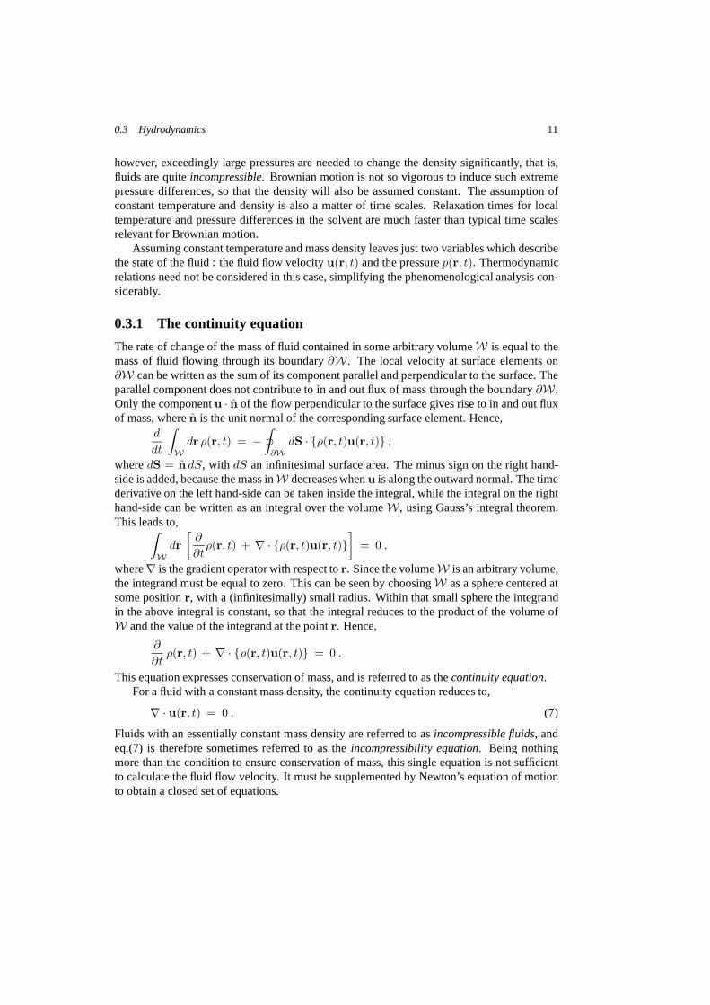
The forces due to interactions with the surrounding fluid areformally expressed in termsof the stress tensorΣ(r, t), which is defined as follows. Consider an infinitesimally smallsurface area in the fluid, with surface areadS and a normal unit vectorn. The force per unitarea exerted by the fluid located at the side of the surface area to which the unit normal isdirected, on the fluid on the opposite side of the surface area, is by definition equal todS · Σ,with dS=n dS (see fig.2).
Hence, by definition, the force of surrounding fluid on the volume elementδr is equal to,∮
∂δr
dS′ · Σ(r′, t) =
∫
δr
dr′ ∇′ · Σ(r′, t) = δr ∇ · Σ(r, t) ,
where∂δr is the boundary of the volume element. We used Gauss’s integral theorem to rewritethe surface integral as a volume integral. The last equationis valid due to the infinitesimal sizeδr of the volume element at positionr. The forcefh on the volume element due to interactionwith the surrounding fluid is thus given by,
fh(r, t) = (δr)∇ ·Σ(r, t) . (8)
There are two contributions to the stress tensor : a contribution resulting from gradients in thefluid flow velocity, and a contribution due to pressure gradients.
Consider first the forces due to pressure gradients. Let us take the volume elementδrcubic, with sides of lengthδl. The pressurep is a force per unit area, so that the force on thevolume element in thex-direction is equal to,
(δl)2(
p(x − 1
2δl, y, z, t)− p(x +
1
2δl, y, z, t)
)
= −(δl)3∂
∂xp(x, y, z, t),
0.3 Hydrodynamics 13
x
y
zdS
),( trSdforcer
tr
S·=
rr
dSnSd ˆ=r
x
y
zdS
),( trSdforcer
tr
S·=
rr
dSnSd ˆ=r
Figure 2: Definition of the stress tensorΣ.
where(δl)2 is the area of the faces of the cube. The force on the volume element is thus−(δr)∇p(r, t). We therefore arrive at,∇ · Σ =−∇p. The contribution of pressure gradientsto the stress tensor is thus easily seen to be equal to,
Σ(r, t) = −p(r, t) I ,
with I the3× 3-dimensional unit tensor. This contribution to the stress tensor is referred to asthe isotropic part of the stress tensor, since it is proportional to the unit tensor and thereforedoes not have a preferred spatial direction.
Next, consider the forces on the volume element due to gradients in the fluid flow veloc-ity. When the fluid flow velocity is uniform, that is, when there are no gradients in the fluidflow velocity, the only forces on the volume element are due topressure and possibly externalforces. There are friction forces in addition, only in case the volume element attains a ve-locity which differs from that of the surrounding fluid. The contribution to the stress tensordue to friction forces is therefore a function of spatial derivatives of the flow velocity, not ofthe velocity itself. This contribution to the stress tensorcan be formally expanded in a powerseries with respect to the gradients in the fluid flow velocity. For not too large gradients (suchthat the fluid velocity is approximately constant over distances of many times the moleculardimension) the leading term in such an expansion suffices to describe friction forces. The con-tribution of gradients in the fluid flow velocity to the stresstensor is thus a linear combinationof the derivatives∇iuj(r, t), where∇i is the derivative with respect to theith component ofr, anduj(r, t) is thejth component ofu(r, t).
There are also no friction forces when the fluid is in uniform rotation, in which case theflow velocity is equal tou = Ω×r, with Ω the angular velocity. Such a fluid flow correspondsto rotation of the vessel containing the fluid, relative to the observer. Linear combinations ofthe form,
∇iuj(r, t) + ∇jui(r, t) , (9)
14
are easily verified to vanish in caseu = Ω × r. The stress tensor is thus proportional to suchlinear combinations of gradients in the fluid velocity field.
For isotropic fluids, with no preferred spatial direction, the most general expression for thecomponentsΣij of the stress tensor as a result of friction is therefore,
ΣD,ij = η0
∇iuj + ∇jui −2
3δij∇ · u(r, t)
+ ζ0 δij∇ · u , (10)
where the subscript “D ” stands forthe deviatoric part of the stress tensor. The terms∼∇ · u(r, t) on the right hand-side are due to the linear combinations (9)with i = j. Theterm− 2
3∇ · u(r, t) is introduced to make the expression between the curly brackets traceless(meaning that the sum of the diagonal elements of that contribution is zero). It could alsohave been absorbed in the last term on the right hand-side. The constantsη0 andζ0, whichare scalar quantities for isotropic fluids, are theshear viscosityandbulk viscosityof the fluid,respectively. Notice that all terms proportional to∇·u(r, t) are zero for incompressible fluids.
We thus find the following expression for the total stress tensor for an isotropic fluid,
Σ(r, t) = η0
∇u(r, t) + [∇u(r, t)]T − 2
3I∇ · u(r, t)
+ ζ0 ∇ · u(r, t) − p(r, t) I , (11)
where the superscriptT stands for transposition.The above expression for the stress tensor leads to theNavier-Stokes equation,
ρ∂u(r, t)
∂t+ ρu(r, t) · ∇u(r, t) = η0 ∇2u(r, t) −∇p(r, t)
+
(
ζ0 +1
3η0
)
∇ (∇ · u(r, t)) + fext(r) , (12)
where the mass density, and the shear- and bulk viscosity arenow taken independent of po-sition. For incompressible fluids, for which∇ · u(r, t) = 0 (see eq.(7)), the Navier-Stokesequation reduces to,
ρ∂u(r, t)
∂t+ρu(r, t)·∇u(r, t) = ∇·Σ(r, t)+fext(r, t) = η0∇2u(r, t)−∇p(r, t)+fext(r).
(13)
Together with the continuity equation (7) for incompressible fluids, this equation fully deter-mines the fluid flow and pressure once the external force and boundary conditions are speci-fied.
0.3.3 The creeping flow equations
The different terms in the Navier-Stokes equation (13) can be very different in magnitude,depending on the problem at hand. In the present case we are interested in fluid flow aroundsmall sized objects (the colloidal particles). Let us estimate the magnitude of the various termsin the Navier-Stokes equation for this case. A typical valuefor the fluid flow velocity is thevelocity v of the colloidal objects. The fluid flow velocity decreases from a valuev, close to
0.3 Hydrodynamics 15
a Brownian particle, to a much smaller value, over a distanceof the order of a typical lineardimensiona of the particles (for spherical particlesa is the radius, for a rotating roda is thelength of the rod). Hence, typically,| ∇2u |≈ v/a2. Similarly, | u · ∇u |≈ v2/a. The rateof change ofu is v divided by the time it takes the colloidal particle to lose its velocity dueto friction with the fluid. This time interval is equal to a fewtimesM/γ, with M the mass ofthe colloidal particle andγ its friction coefficient (this will be discussed in more detail later inthis chapter). Introducing the rescaled variables,
u′ = u/v ,
r′ = r/a ,
t′ = t/(M/γ) ,
transforms the Navier-Stokes equation (13) to,
ρ γ v
M
∂u′
∂t′+
ρ v2
au′ · ∇′u′ =
η0v
a2∇′ 2u′ − 1
a∇′p + fext ,
where∇′ is the gradient operator with respect tor′. Introducing further the dimensionlesspressure and external force,
p′ =a
η0vp ,
f ′ ext =a2
η0vfext ,
transforms the Navier-Stokes equation further to,
ρa2γ
Mη0
∂u′
∂t′+ Re u′ · ∇′u′ = ∇′ 2u′ −∇′p′ + f ′ ext . (14)
The dimensionless numberRe is the so-calledReynolds number, which is equal to,
Re =ρ a v
η0. (15)
By construction we have,
| u′ · ∇′u′ | ≈ | ∇′ 2u′ | ≈ 1.
Hence, for very small values of the Reynolds number, the termproportional tou · ∇u inthe left hand-side in eq.(14) may be neglected. Furthermore, for spherical particles we haveγ = 6πη0a so thatρ a2γ/Mη0 = 9ρ/2ρp ≈ 9/2, with ρp the mass density of the Brownianparticle. The prefactor of∂u′/∂t′ is thus approximately equal to9/2. The time deriva-tive should generally be kept as it stands, also for small Reynolds numbers. Now suppose,however, that one is interested in a description on the diffusive time scaleτD ≫ M/γ (thesignificance of the diffusive time scale will be discussed later in this chapter). For such times,the time derivative∂u′/∂t′ is long zero, sinceu goes to zero as a result of friction during thetime intervalM/γ. One may then neglect the contribution to the time derivative which is dueto relaxation of momentum of the Brownian particle as a result of friction with the solvent.The remaining time dependence ofu on the diffusive time scale is due to the possible timedependence of the external force and to interactions with other Brownian rods, which vary

16
significantly only over time intervals larger than the diffusive time scale. The value of thecorresponding derivative∂u/∂t can now be estimated as above : the only difference is thatthe time should not be rescaled with respect to the timeM/γ, but with respect to the diffusivetime scaleτD. We now have,t′ = t/τD, u′ = u/v, and| ∂u′/∂t′ |≈ 1. The transformedNavier-Stokes equation in this case reads,
9
2
ρ
ρp
M/γ
τD
∂u′
∂t′+ Re u′ · ∇′u′ = ∇′ 2u′ −∇′p′ + f ′ ext ,
where all derivatives of the fluid flow velocityu′ are of the order1. SinceτD ≫ M/γ, thetime derivative due to changes of the fluid flow velocity as a result of the time varying externalforce and interactions with other Brownian particles may now be neglected in addition.
For small Reynolds numbers and on the diffusive time scale, the Navier-Stokes equation(16), written in terms of the original unprimed quantities,therefore simplifies to,
∇p(r, t) − η0∇2 u(r, t) = fext(r) . (16)
This equation, together with the incompressibility equation (7), are thecreeping flow equa-tions. “Creeping” refers to the fact that the Reynolds number is small, which is the case whenthe typical fluid flow velocityv is small.
A typical value for the velocity of a Brownian particle can beestimated from the equipar-tition theorem,12M < v2 >= 3
2kBT (kB is Boltzmann’s constant andT is the temperature).Estimatingv ≈
√<v2 >, using a typical mass of10−17 kg for a spherical particle with a
radius of100 nm and the density and viscosity of water, the Reynolds number is found to beequal to10−2. Hydrodynamics of a fluid in which colloidal particles are embedded can thusbe described on the basis of the creeping flow equations.
For small Reynolds numbers and on the Brownian time scale, inertial forces on fluid el-ements are thus small in comparison to pressure- and friction forces. The neglect of inertialcontributions in the Navier-Stokes equation leads to the linear equation (16), which can besolved analytically in some cases.
0.3.4 The Oseen tensor
An external force acting only in a single pointr′ on the fluid is mathematically described by adelta distribution,
fext(r) = f0 δ(r − r′) . (17)
The prefactorf0 is the total force∫
dr′ fext(r′) acting on the fluid. Since the creeping flowequations are linear, the fluid flow velocity at some pointr in the fluid, due to the point forcein r′, is directly proportional to that point force. Hence,
u(r) = T(r − r′) · f0 .
The tensorT is commonly referred to as theOseen tensor, named after the scientist who firstderived an explicit expression for this tensor, Oseen (1927). The Oseen tensor connects thepoint force at a pointr′ to the resulting fluid flow velocity at a pointr. Note thatT is only a
0.3 Hydrodynamics 17
function of the difference coordinater − r′ due to translational invariance of a homogeneousfluid. Similarly, the pressure at a pointr is linearly related to the point force,
p(r) = g(r − r′) · f0 .
The vectorg is referred to here as thepressure vector.Consider an external force which is continuously distributed over the entire fluid. Due to
the linearity of the creeping flow equations, the fluid flow velocity at some pointr is simplythe superposition of the fluid flow velocities resulting fromthe forces acting in each point onthe fluid. Hence,
u(r) =
∫
dr′ T(r − r′) · fext(r′) . (18)
The same holds for the pressure,
p(r) =
∫
dr′ g(r − r′) · fext(r′) . (19)
In mathematical language, the Oseen tensor and the pressurevector are the Green’s functionsof the creeping flow equations for the fluid flow velocity and pressure, respectively. Once theseGreen’s functions are known and the external force is specified, the resulting fluid velocity andpressure can be calculated through the evaluation of the above integrals. The calculation ofthe Green’s functions is thus equivalent to solving the creeping flow equations, provided thatthe external forces are known.
Let us calculate the Oseen tensor and pressure vector. To this end, substitute eqs.(18,19)into the creeping flow equations (7,16). This leads to,
∫
dr′ [∇ ·T(r − r′)] · fext(r′) = 0 ,
∫
dr′[
∇g(r − r′) − η0∇2T(r − r′) − I δ(r − r′)]
· fext(r′) = 0 ,
where, as before,I is the3 × 3-dimensional unit tensor. Since the external force is arbitrary,the expressions in the square brackets must be equal to zero,so that the Green’s functionssatisfy the following differential equations,
∇ · T(r) = 0 ,
∇g(r) − η0∇2T(r) = I δ(r) . (20)
A single equation for the pressure vector is obtained by taking the divergence of the secondequation, with the use of the first equation,
∇2 g(r) = ∇ · I δ(r) = ∇δ(r) .
Using,
1
4π∇2 1
r= − δ(r) , (21)
18
it follows that,
g(r) = − 1
4π∇1
r+ G(r) .
Here,G is a vector for which∇2G=0, whileG → 0 asr → ∞. It can be shown that such avector is0. Hence,
g(r) = − 1
4π∇1
r=
1
4π
r
r3. (22)
The differential equation to be satisfied by the Green’s function for the fluid flow velocity (theOseen tensor), is found by substitution of eq.(22) into eq.(20),
∇2
[
1
4π
1
rI − η0T(r)
]
=1
4π
[
3r r
r5− 1
r3I
]
.
An obvious choice for the term between the square brackets onthe left hand-side of the aboveexpression is of the form,
1
4π
1
rI− η0T(r) = α0
1
rnI + α1
1
rm
r r
r2,
with α0,1, n andm constants. These constants can indeed be chosen such that this Ansatzis the solution of the differential equation (with the boundary condition thatT(r) → 0 asr → ∞). A somewhat lengthy, but straightforward calculation yields,
T(r) =1
8πη0
1
r
[
I +r r
r2
]
. (23)
This concludes the determination of the Green’s functions for the creeping flow equations.
0.4 Hydrodynamic Friction of a Single Rod
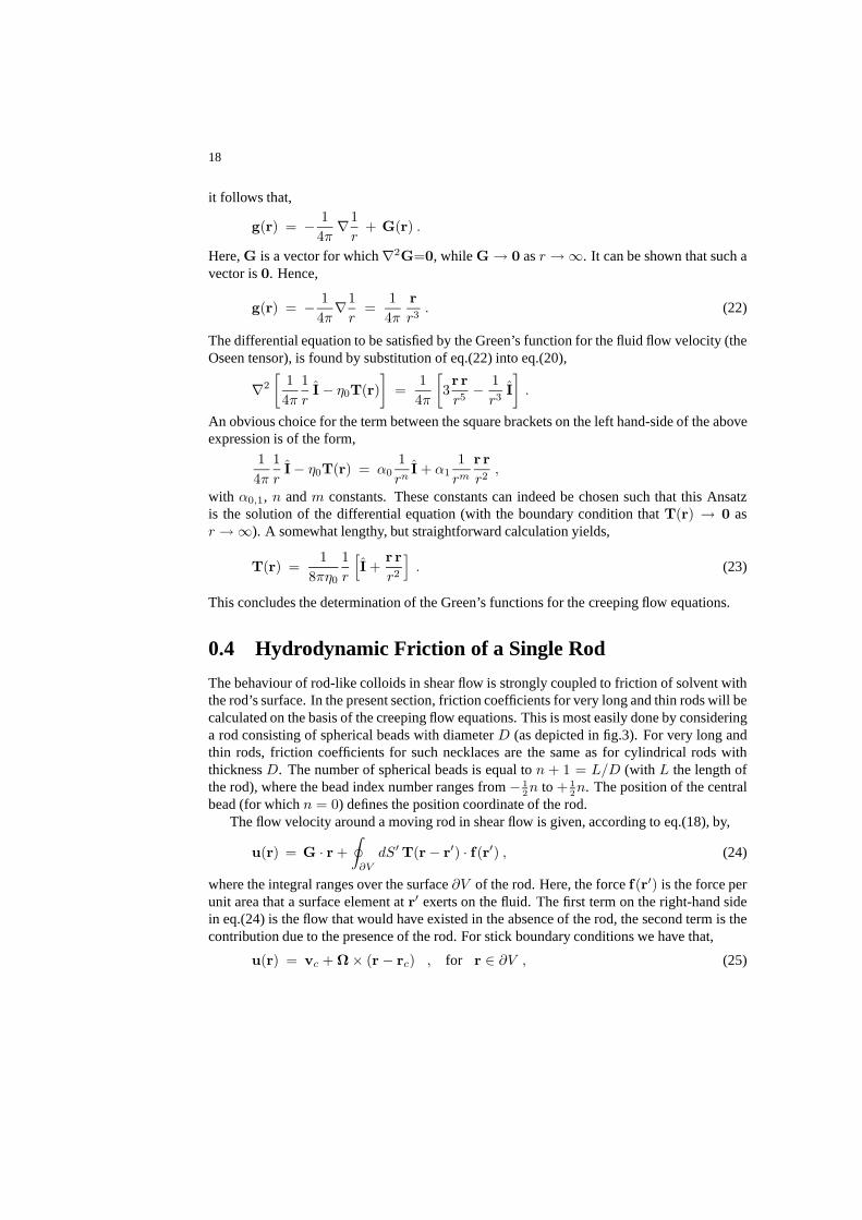
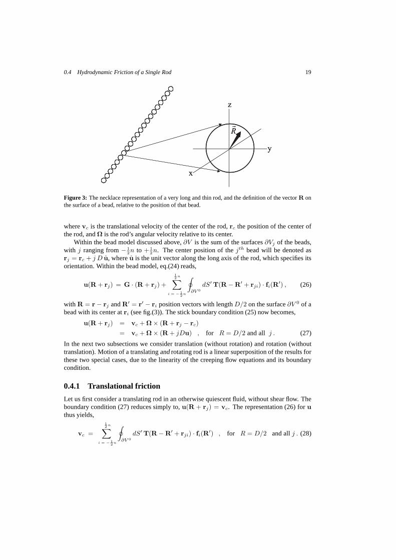
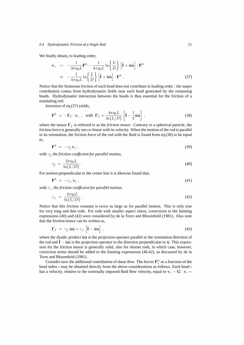
The behaviour of rod-like colloids in shear flow is strongly coupled to friction of solvent withthe rod’s surface. In the present section, friction coefficients for very long and thin rods will becalculated on the basis of the creeping flow equations. This is most easily done by consideringa rod consisting of spherical beads with diameterD (as depicted in fig.3). For very long andthin rods, friction coefficients for such necklaces are the same as for cylindrical rods withthicknessD. The number of spherical beads is equal ton + 1 = L/D (with L the length ofthe rod), where the bead index number ranges from− 1
2n to + 1
2n. The position of the central
bead (for whichn = 0) defines the position coordinate of the rod.The flow velocity around a moving rod in shear flow is given, according to eq.(18), by,
u(r) = G · r +
∮
∂V
dS′ T(r − r′) · f(r′) , (24)
where the integral ranges over the surface∂V of the rod. Here, the forcef(r′) is the force perunit area that a surface element atr′ exerts on the fluid. The first term on the right-hand sidein eq.(24) is the flow that would have existed in the absence ofthe rod, the second term is thecontribution due to the presence of the rod. For stick boundary conditions we have that,
u(r) = vc + Ω× (r − rc) , for r ∈ ∂V , (25)
0.4 Hydrodynamic Friction of a Single Rod 19
x
y
z
Rr
x
y
z
Rr
Figure 3: The necklace representation of a very long and thin rod, and the definition of the vectorR onthe surface of a bead, relative to the position of that bead.
wherevc is the translational velocity of the center of the rod,rc the position of the center ofthe rod, andΩ is the rod’s angular velocity relative to its center.
Within the bead model discussed above,∂V is the sum of the surfaces∂Vj of the beads,with j ranging from− 1
2n to + 1
2n. The center position of thejth bead will be denoted as
rj = rc + j D u, whereu is the unit vector along the long axis of the rod, which specifies itsorientation. Within the bead model, eq.(24) reads,
u(R + rj) = G · (R + rj) +
12
n∑
i = − 12
n
∮
∂V 0
dS′ T(R − R′ + rji) · fi(R′) , (26)
with R = r − rj andR′ = r′ − ri position vectors with lengthD/2 on the surface∂V 0 of abead with its center atri (see fig.(3)). The stick boundary condition (25) now becomes,
u(R + rj) = vc + Ω× (R + rj − rc)
= vc + Ω× (R + jDu) , for R = D/2 and all j . (27)
In the next two subsections we consider translation (without rotation) and rotation (withouttranslation). Motion of a translatingandrotating rod is a linear superposition of the results forthese two special cases, due to the linearity of the creepingflow equations and its boundarycondition.
0.4.1 Translational friction
Let us first consider a translating rod in an otherwise quiescent fluid, without shear flow. Theboundary condition (27) reduces simply to,u(R + rj) = vc. The representation (26) foruthus yields,
vc =
12
n∑
i = − 12
n
∮
∂V 0
dS′ T(R − R′ + rji) · fi(R′) , for R = D/2 and allj . (28)

20
Integration of both sides over the surface of the entire rod,that is, operating on both sides with∑
12
n
j = − 12
n
∮
∂V 0 dS, yields,
vc =1
πLD
12
n∑
j = − 12
n
12
n∑
i = − 12
n
∮
∂V 0
dS
∮
∂V 0
dS′ T(R − R′ + rji) · fi(R′) . (29)
Using that,∮
∂V 0
dS′ T(r − R′) =D
4 η0
[
D
2r+
1
3
(
D
2r
)3]
I +
[
D
2r−
(
D
2r
)3]
rr
r2
, (30)
it is found that, fori = j, the surface integrals in eq.(29) are equal to,∮
∂V 0
dS T(R − R′ + rji) =D
3η0I , for i = j . (31)
For i 6= j, the Oseen tensor may be Taylor expanded as,
T(R − R′ + rji) = T(rij) + (R − R′) · ∇iT(rij) + · · · , (32)
with ∇i the gradient operator with respect tori. Only the leading order term in this Taylorexpansion must be retained to obtain expressions for friction coefficients that are valid toleading order inL/D (if you wish you may include the next higher order Taylor terms andconvince yourself that these terms do not contribute in leading order). Using eq.(31) andeq.(32) to leading order in eq.(29) gives,
vc ≈ − 1
3πη0L
12
n∑
i = − 12
n
Fhi − D
L
12
n∑
j = − 12
n
12
n∑
i = − 12
n , i 6= j
T(rij)
· Fhi . (33)
where,∮
∂V 0
dS′ fi(R′) = −Fh
i , (34)
is the total force of the fluid on beadi. The first term on the right-hand side is simply the sumof Stokesian friction forces on the beads, while the second term represents the contributiondue to hydrodynamic interaction between the beads. For verylong rods, all forcesFh
i may betaken equal, that is, end-effects may be neglected, since the majority of beads (away from theends of the rod) experience approximately the same force. SubstitutingFh
i = DL Fh, with Fh
the total force on the rod, yields,
vc = − 1
3πη0LFh −
(
D
L
)2
12
n∑
j = − 12
n
12
n∑
i = − 12
n , i 6= j
T(rij)
· Fh . (35)
The double bead index summation can be calculated up to leading order by replacing sums byintegrals (for details see appendix A). It is thus found that,
12
n∑
j = − 12
n
12
n∑
i = − 12
n , i 6= j
T(rij) =1
8πη0D
[
I + uu]
12
n∑
j = − 12
n
12
n∑
i = − 12
n , i 6= j
1
| i − j |
≈ 1
4πη0D
[
I + uu] L
Dln
L
D
. (36)
0.4 Hydrodynamic Friction of a Single Rod 21
We finally obtain, to leading order,
vc = − 1
3πη0LFh − 1
4πη0Lln
L
D
[
I + uu]
·Fh
≈ − 1
4πη0Lln
L
D
[
I + uu]
· Fh . (37)
Notice that the Stokesian friction of each bead does not contribute in leading order : the majorcontribution comes from hydrodynamic fields near each bead generated by the remainingbeads. Hydrodynamic interaction between the beads is thus essential for the friction of atranslating rod.
Inversion of eq.(37) yields,
Fh = −Γf · vc , with Γf =4πη0L
lnL/D
[
I − 1
2uu
]
, (38)
where the tensorΓf is referred to as thefriction tensor. Contrary to a spherical particle, thefriction force is generally not co-linear with its velocity. When the motion of the rod is parallelto its orientation, the friction force of the rod with the fluid is found from eq.(38) to be equalto,
Fh = −γ‖ vc , (39)
with γ‖ the friction coefficient for parallel motion,
γ‖ =2πη0L
lnL/D . (40)
For motion perpendicular to the center line it is likewise found that,
Fh = −γ⊥ vc , (41)
with γ⊥ the friction coefficient for parallel motion,
γ⊥ =4πη0L
lnL/D . (42)
Notice that this friction constant is twice as large as for parallel motion. This is only truefor very long and thin rods. For rods with smaller aspect ratios, corrections to the limitingexpressions (40) and (42) were considered by de la Torre and Bloomfield (1981). Also notethat the friction tensor can be written as,
Γf = γ‖ uu + γ⊥
[
I − uu]
, (43)
where the dyadic productuu is the projection operator parallel to the orientation direction ofthe rod andI− uu is the projection operator in the direction perpendicular to u. This expres-sion for the friction tensor is generally valid, also for shorter rods, in which case, however,correction terms should be added to the limiting expressions (40,42), as discussed by de laTorre and Bloomfield (1981).
Consider now the additional contribution of shear flow. The forcesFhi as a function of the
bead indexi may be obtained directly from the above considerations as follows. Each beadihas a velocity, relative to the externally imposed fluid flow velocity, equal tovc − G · ri =

22
vc−G ·rc−iDG ·u. Therelativechange of this velocity between neighbouring beads is thus∼ 1/i, and is small for beads away from the center. Large groups of beads therefore experiencea friction force as in the case of a uniformly translating rodin an otherwise quiescent fluid.Beads away from the center therefore experience a friction force parallel to the center lineequal to,
Fhi , ‖ = −D
Lγ‖ uu · (vc − G · rc − iDG · u) ,
and perpendicular to the center line,
Fhi , ⊥ = −D
Lγ⊥
[
I− uu]
· (vc − G · rc − iDG · u) .
Here, the apparent local velocity of the fluid is decomposed in its component parallel andperpendicular to the rods center line, and the friction coefficient on the bead is equal to thatof an entire rod divided by the numbern + 1 = L/D of beads. The total force that the fluidexerts on the rod is now simply found by summation over all beads,
Fh =
12
n∑
i = − 12
n
[
Fhi , ‖ + Fh
i , ⊥
]
= −(
γ‖uu + γ⊥
[
I− uu])
· (vc − G · rc)
= − 4πη0L
ln L/D
[
I− 1
2uu
]
· (vc − G · rc) . (44)
The last equation is only valid for very long and thin rods. The first equation is also valid forshorter rods, where expressions for the two friction coefficients were calculated by de la Torreand Bloomfield (1981). This result is precisely eq.(38) for translational motion in an otherwisequiescent fluid, where the velocity of the rods center is taken relative to the local shear flowvelocity. Such a result is intuitively clear, as additionalfriction forces due to the shear flowon the beads with a positive bead index simply cancel with thesame forces on beads with anegative index.
0.4.2 Rotational friction
Consider a rod in shear flow with its center at the origin (so that vc = 0 = rc) and with aprescribed angular velocityΩ perpendicular to its center line. The rotational friction coeffi-cient may be obtained directly from the above results on translational friction, with argumentssimilar to the ones given at the end of the previous subsection where the effect of shearingmotion of the fluid on translational friction is considered.The velocity of beadi relative tothe local fluid flow velocity is equal toΩ×ri − G · ri = iD Ω × u − −iD G · u. Therelativechange of this velocity between neighbouring beads is thus∼ 1/i, and is small forbeads away from the origin. Large groups of beads therefore experience a friction force asin case of a uniformly translating rod in an otherwise quiescent fluid. Beads away from theorigin therefore experience a friction force parallel to the center line equal to,
Fhi , ‖ = −D
Lγ‖ uu · (iD Ω× u − iD G · u) , (45)
0.4 Hydrodynamic Friction of a Single Rod 23
force
force
force
force
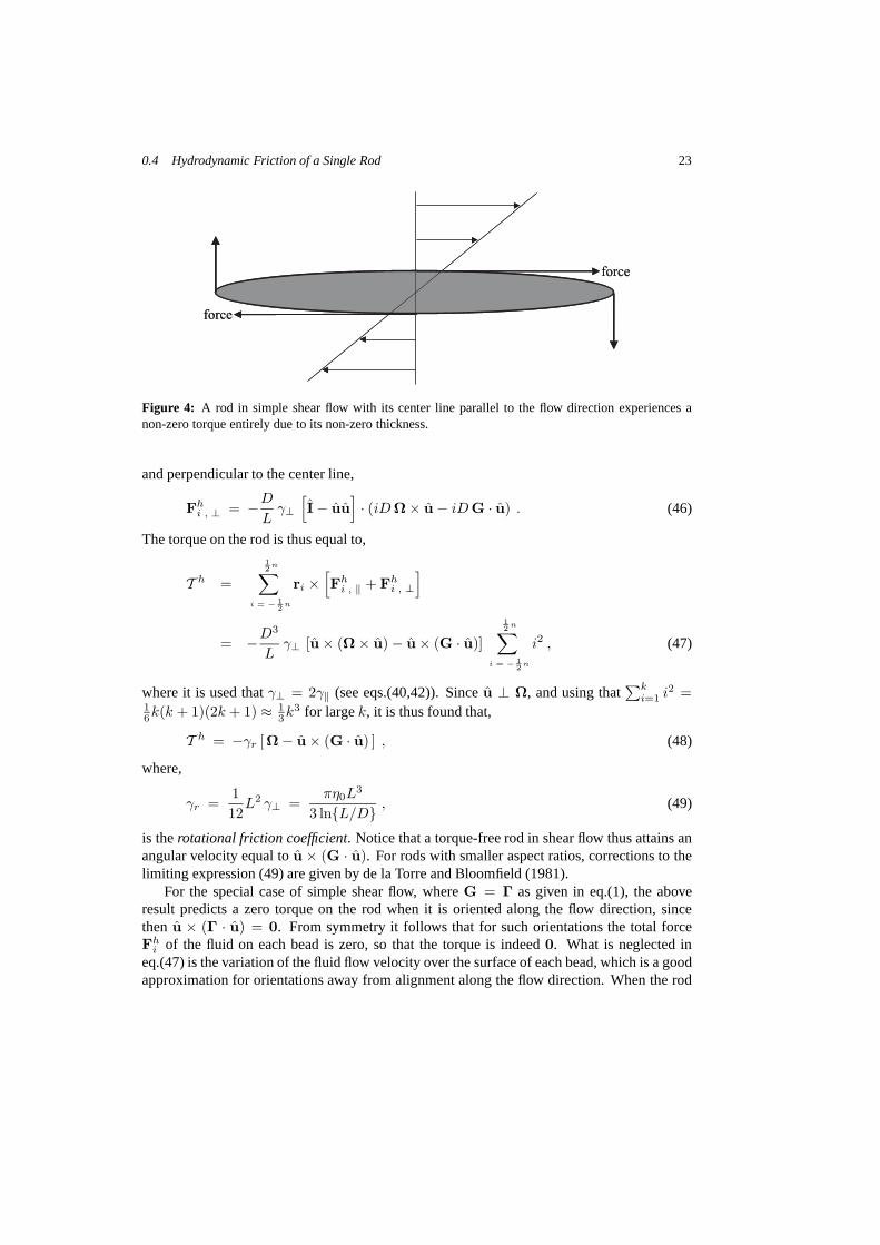
Figure 4: A rod in simple shear flow with its center line parallel to the flow direction experiences anon-zero torque entirely due to its non-zero thickness.
and perpendicular to the center line,
Fhi , ⊥ = −D
Lγ⊥
[
I − uu]
· (iD Ω× u − iD G · u) . (46)
The torque on the rod is thus equal to,
T h =
12
n∑
i = − 12
n
ri ×[
Fhi , ‖ + Fh
i , ⊥
]
= −D3
Lγ⊥ [u× (Ω × u) − u× (G · u)]
12
n∑
i = − 12
n
i2 , (47)
where it is used thatγ⊥ = 2γ‖ (see eqs.(40,42)). Sinceu ⊥ Ω, and using that∑k
i=1 i2 =16k(k + 1)(2k + 1) ≈ 1
3k3 for largek, it is thus found that,
T h = −γr [Ω − u× (G · u) ] , (48)
where,
γr =1
12L2 γ⊥ =
πη0L3
3 lnL/D , (49)
is therotational friction coefficient. Notice that a torque-free rod in shear flow thus attains anangular velocity equal tou × (G · u). For rods with smaller aspect ratios, corrections to thelimiting expression (49) are given by de la Torre and Bloomfield (1981).
For the special case of simple shear flow, whereG = Γ as given in eq.(1), the aboveresult predicts a zero torque on the rod when it is oriented along the flow direction, sincethen u × (Γ · u) = 0. From symmetry it follows that for such orientations the total forceFh
i of the fluid on each bead is zero, so that the torque is indeed0. What is neglected ineq.(47) is the variation of the fluid flow velocity over the surface of each bead, which is a goodapproximation for orientations away from alignment along the flow direction. When the rod
24
is oriented along the flow direction, however, the fluid flow variation over the surfaces of thebeads give rise to a small but non-zero torque. The torque is only non-zero when the finitethickness of the rod is taken into account, and its magnitudeis at least an orderD/L smallerthan the torqueγru × (Γ · u) for orientations not parallel to the flow direction.
As will be seen in the section on Jeffery orbits, which are theorbits described byu ofa non-Brownian rod in shear flow, the small torque on a rod thatis oriented along the flowdirection is essential to obtain the realistic periodic motion for u : without this small contri-bution,u would simply end up in the direction parallel to the flow. Let us therefore considerthis small, but essential contribution to the torque for non-Brownian rods.
The additional contribution to the torque is due to variations of the fluid forces over thebead surfaces. Taking these variations into account, the torque is by definition equal to (∂V isagain the surface of the rod),
T h = −∮
∂V
dS′ r′ × f(r′) = −12
n∑
i = − 12
n
∮
∂V 0
dS′ (R′ + ri) × fi(R′)
=
12
n∑
i = − 12
n
ri × Fhi −
12
n∑
i = − 12
n
∮
∂V 0
dS′ R′ × fi(R′) . (50)
The last term on the right-hand side is now extra as compared to the case where the additionaltorque due to variations of the hydrodynamic forces over therods surface is neglected. Thisis the term that is responsible for a finite torque when the rodis oriented along the flowdirection. The first term on the right-hand side is already considered before with the neglectof end-effects. In calculating the additional contribution ∆T h (the last term on the right-handside) end-effects will also be neglected, meaning that the variation of the hydrodynamic forcesover the bead surface is taken equal for all beads. The variation of the fluid flow in which abead is embedded is given byΓ · R′. We are only interested in the component of this flow inthe direction alongu, since the complementary perpendicular component gives rise to rotationabout the center line, which does not affectu. This parallel component of the flow along thesurface of the rod is equal touu · Γ · R′, and the corresponding parallel force is proportionalto this flow velocity. Hence,
fi(R′) = C uu · Γ ·R′ , (51)
whereC is an as yet unknown constant. It now follows that,
∆T h = −C
12
n∑
i = − 12
n
∮
∂V 0
dS′ R′ × (Γ ·R′) = CL
D
πD4
12u ×
(
ΓT · u)
, (52)
where the superscript “T ” stands for transposition. The constantC can now be determinedby comparing this result to solutions of the creeping flow equations for the simple case thatthe rod is oriented along the flow direction. For the case of a cylinder without end-effects andfor a long and thin ellipsoidal particles it can be shown that,
C = −6 η0
D, for cylinders without end-effects, (53)
= − 4 η0
D lnL/D , for long and thin ellipsoids. (54)

0.5 Motion of Non-Brownian Rods in Shear Flow : Jeffery Orbits 25
The different results are not just the result of neglect of end-effects in case of the cylindricalparticle. The precise value ofC is sensitive to the precise shape of the surface of the rod : thetorque on a rod aligned along the flow direction depends on howthe fluid is “pushed away” or“sucked in” as it flows along its surface.
We thus finally find the following expression for the torque,
T h = −γr
[
Ω− u × (Γ · u) + κ2 u ×(
ΓT · u) ]
, (55)
where the dimensionless constantκ2 is equal to,
κ2 =3
2
(
D
L
)2
ln
L
D
, for cylinders without end-effects, (56)
=
(
D
L
)2
, for long and thin ellipsoids . (57)
Since for colloidal rods the precise geometry of their surface is usually not known, andκ2 issensitive to that geometry, the constantκ2 should be considered as a fitting parameter whenperforming experiments. This parameter tends to zero with decreasing values ofD/L.
0.5 Motion of Non-Brownian Rods in Shear Flow :Jeffery Orbits
The first thing that comes to mind when beginning to study the effect of shear flow on di-lute suspensions of rods is to ask about their motion withoutconsidering Brownian motion.The trajectory of motion of a Brownian rod will be the smooth trajectory of a non-Brownianrod that is randomly corrugated due to Brownian motion. In this section we ask for the ori-entational orbits that a non-Brownian rod (a “fiber”) traverses when subjected to shear flow.These orbits are commonly the referred to asJeffery orbits, named after the scientist Jefferey(1922) who first considered this problem (a more compact formulation as compared to theoriginal work of Jeffery has been formulated by Hinch and Leal (1972) and Leal and Hinch(1972)). We shall consider Jeffery orbits of rods in elongational flow and simple shear flow,respectively.
The expressions derived in the previous section for very long and thin rods will be usedto calculate such Jeffery orbits. Jefferey (1922) derived exact expressions for ellipsoidal rods,while Bretherton (1962) showed that the same equations of motion can be applied to arbi-trary shaped, cylindrically symmetric, slender bodies, provided that the body is modelled asan equivalent ellipsoid. The expressions obtained in the following are the asymptotic limitsfor large aspect ratios of those derived by Jeffery and Bretherton. It turns out, however, thatfor aspect ratiosL/D larger than about3-4, errors that are made in using these asymptotic ex-pressions (but employing the correct value for the rotational friction coefficient) are typicallyless about5% (asymptotic limits are obtained when, typically,1/(1 + r2) is approximated by1/r2, wherer = L/D). This is confirmed by simulations (see for example Ingber and Mondy(1994)).
Interactions between fibers at high fiber concentration and intrinsic flexibility of fibersdoes of course have an effect on the orbits described by a rod.Simulations on Jeffery orbits
26
x
y
z
Q
j
Figure 5: Definition of the spherical coordinatesϕ andΘ, relative to the flow and gradient direction incase of simple shear flow. The flow is in thex-direction while the gradient is in they-direction. In thisexample,ϕ < 0.
where interactions and flexibility are considered have beenperformed by Yamamoto and Mat-suoka (1995). The theory described here assumes rigid rods.A discussion and references onthe effect of interactions between fibers, wall effects and rheology of fiber suspensions canbe found in the book by Papathanasiou and Guell (1997). The treatment here describes themotion of a single fiber, which is not affected by interactions with other fibers or a wall.
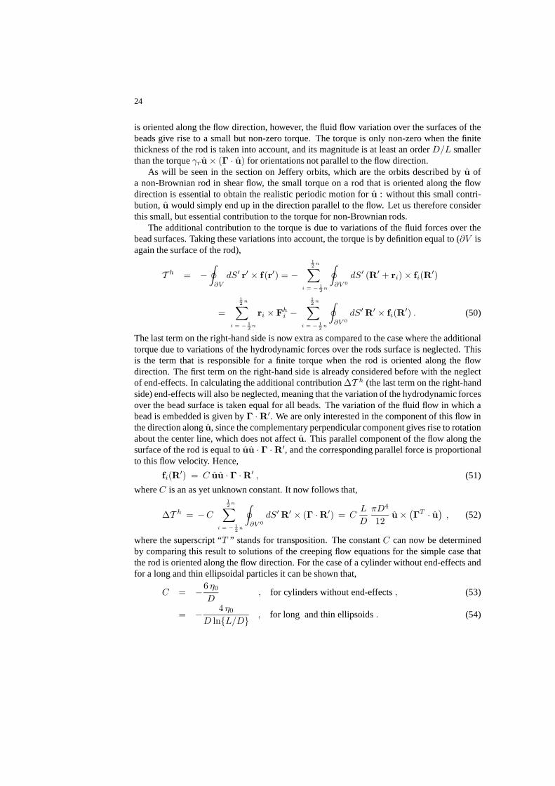
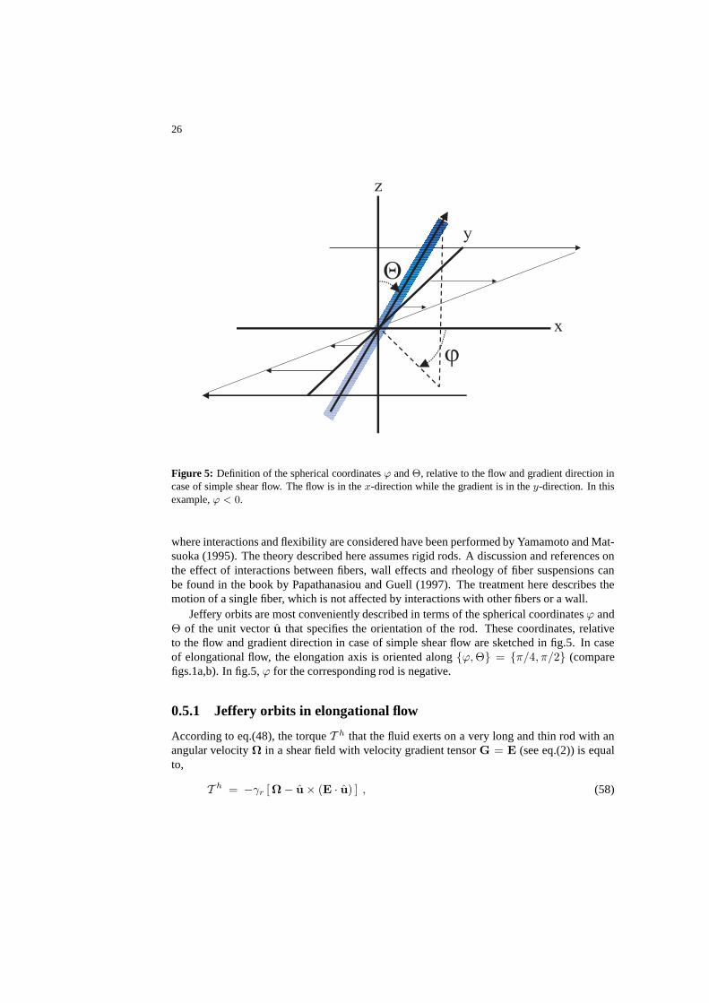
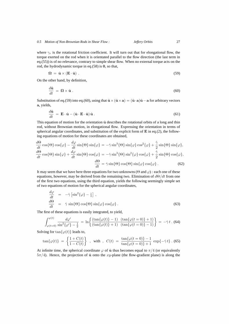
Jeffery orbits are most conveniently described in terms of the spherical coordinatesϕ andΘ of the unit vectoru that specifies the orientation of the rod. These coordinates, relativeto the flow and gradient direction in case of simple shear flow are sketched in fig.5. In caseof elongational flow, the elongation axis is oriented alongϕ, Θ = π/4, π/2 (comparefigs.1a,b). In fig.5,ϕ for the corresponding rod is negative.
0.5.1 Jeffery orbits in elongational flow
According to eq.(48), the torqueT h that the fluid exerts on a very long and thin rod with anangular velocityΩ in a shear field with velocity gradient tensorG = E (see eq.(2)) is equalto,
T h = −γr [Ω− u × (E · u) ] , (58)
0.5 Motion of Non-Brownian Rods in Shear Flow : Jeffery Orbits 27
whereγr is the rotational friction coefficient. It will turn out thatfor elongational flow, thetorque exerted on the rod when it is orientated parallel to the flow direction (the last term ineq.(55)) is of no relevance, contrary to simple shear flow. When no external torque acts on therod, the hydrodynamic torque in eq.(58) is0, so that,
Ω = u× (E · u) . (59)
On the other hand, by definition,
du
dt= Ω× u . (60)
Substitution of eq.(59) into eq.(60), using thatu× (u×a) = (u ·a)u−a for arbitrary vectorsa, yields,
du
dt= E · u− (u · E · u) u . (61)
This equation of motion for the orientationu describes the rotational orbits of a long and thinrod, without Brownian motion, in elongational flow. Expressing the orientation in terms ofspherical angular coordinates, and substitution of the explicit form of E in eq.(2), the follow-ing equations of motion for these coordinates are obtained,
dΘ
dtcosΘ cosϕ − dϕ
dtsinΘ sinϕ = −γ sin3Θ sinϕ cos2ϕ +
γ
2sinΘ sinϕ,
dΘ
dtcosΘ sinϕ +
dϕ
dtsinΘ cosϕ = −γ sin3Θ sin2ϕ cosϕ +
γ
2sinΘ cosϕ,
dΘ
dt= γ sinΘ cosΘ sinϕ cosϕ . (62)
It may seem that we have here three equations for two unknowns(Θ andϕ) : each one of theseequations, however, may be derived from the remaining two. Elimination ofdΘ/dt from oneof the first two equations, using the third equation, yields the following seemingly simple setof two equations of motion for the spherical angular coordinates,
dϕ
dt= −γ
[
sin2ϕ − 12
]
,
dΘ
dt= γ sinΘ cosΘ sinϕ cosϕ . (63)
The first of these equations is easily integrated, to yield,∫ ϕ(t)
ϕ(t=0)
dϕ′
sin2ϕ′ − 12
= ln
(tanϕ(t) − 1) (tanϕ(t = 0) + 1)
(tanϕ(t) + 1) (tanϕ(t = 0) − 1)
= −γ t . (64)
Solving fortanϕ(t) leads to,
tanϕ(t) =
1 + C(t)
1 − C(t)
, with , C(t) =tanϕ(t = 0) − 1
tanϕ(t = 0) + 1exp−γ t . (65)
At infinite time, the spherical coordinateϕ of u thus becomes equal toπ/4 (or equivalently5π/4). Hence, the projection ofu onto thexy-plane (the flow-gradient plane) is along the

28
0 30 60 900
15
30
45
p/4 p/2p/3p/8
j(a)
q(t=0)=p/100
q
0 30 60 90
-540
-360
-180
0
10p/23 10p/21 100p/205p/3
p/8
j (b)
q(t=0)=
p/100
q
Figure 6: (a) Jeffery orbits for elongational flow for initial valuesϕ(t = 0) = π/100 and various valuesfor Θ(t = 0), as indicated in the figure. Data points• correspond to time steps equal to1/(10 γ). Thearrows indicate the direction of the temporal evolution of the spherical coordinates. (b) Jeffery orbits forsimple shear flow withκ = 0.1, for various values ofΘ(t = 0), as indicated in the figure. The points•on the orbits mark time intervals ofT/200. ϕ(t) decreases with time.
0.5 Motion of Non-Brownian Rods in Shear Flow : Jeffery Orbits 29
direction of the the extensional axis of the elongational flow. The reason for this is easilyinferred from fig.1b.
Dividing the two equations of motion in eq.(63) yields,
dΘ
sinΘ cosΘ = − dϕ sinϕ cosϕsin2ϕ − 1
2
.
Integration of both sides now leads to,
tanΘ(t) = tanΘ(t = 0)√
sin2ϕ(t = 0) − 12
sin2ϕ(t) − 12
, (66)
whereϕ(t) can be obtained from eq.(65). Sinceϕ(t) tends toπ/4 (or 5π/4), the abovesolution predicts thattanΘ tends to infinity, and henceΘ(t) → π/2. Hence, independentof the initial condition, a rod will end up in the velocity-gradient plane along the extensionalaxis. This is verified in fig.6a, which shows numerical results for the spherical coordinates.Here, the distance between each data point is1/(10 γ). Data are shown for small values ofϕ(t = 0). For larger initial values forϕ, the orbit just starts on one of the curves shownand then traces the same orbit. As can be seen from the most upper-left curve in fig.6a,when the initial value ofΘ is small, the rod spends a relatively long time around the unstablestationary solutionΘ, ϕ = 0, π/4 of the equations of motion, before reaching the finalstable stateΘ, ϕ = π/2, π/4. That is,u first rotates to the extensional direction whereϕ = π/4, keeping its angleΘ with the vorticity direction relatively small. This angle thenslowly increases, after which there is an acceleration towards the final orientation.
0.5.2 Jeffery orbits in simple shear flow
As we have seen in the section on hydrodynamics, the torqueT h that the fluid exerts on avery long and thin rod with an angular velocityΩ in a shear field with velocity gradient tensorG = Γ (see eq.(1)) is equal to,
T h = −γr
[
Ω− u × (Γ · u) + κ2 u ×(
ΓT · u) ]
, (67)
whereγr is the rotational friction coefficient. The parameterκ2 tends to zero for decreasingvalues ofD/L, and measures the torque of the rod when aligned such thatϕ = 0, for whichcaseu× (Γ · u) = 0. Neglecting this small contribution results in an orientation of the rod inthe flow direction for long times, while for a rod of finite thickness, whereκ2 is small but non-zero, a periodic motion results. Contrary to the case of elongational flow, considered in theprevious subsection, the small but finite contribution∼ κ2 is essential for a correct descriptionin case of simple shear flow.
When no other torque is acting on the rod, the hydrodynamic torque is0, so that,
Ω = u× (Γ · u) − κ2 u×(
ΓT · u)
. (68)
Precisely as for elongational flow, this implies that,
du
dt= Γ · u − κ2 ΓT · u− (u · Γ · u) u . (69)

30
In terms of spherical coordinates, this is equivalent to,
dΘ
dtcosΘ cosϕ− dϕ
dtsinΘ sinϕ=−γ(1−κ2) sin3Θ sinϕ cos2ϕ+γ sinΘ sinϕ,
dΘ
dtcosΘ sinϕ+
dϕ
dtsinΘ cosϕ=−γ(1−κ2) sin3Θ sin2ϕ cosϕ−γκ2 sinΘ cosϕ,
dΘ
dt= γ(1−κ2) sinΘ cosΘ sinϕ cosϕ . (70)
Precisely as in the previous case of elongational flow, we thus arrive at the following equationsof motion for the spherical angular coordinates,
dϕ
dt= −γ
[
sin2ϕ + κ2 cos2ϕ]
,
dΘ
dt= γ(1 − κ2) sinΘ cosΘ sinϕ cosϕ . (71)
The first of these equations is easily integrated to yield,∫ ϕ(t)
ϕ(t=0)
dϕ′
sin2ϕ′ + κ2 cos2ϕ′ =1
κ
[
arctan
1
κtanϕ(t)
− C′
]
= −γ t , (72)
whereC′ is an integration constant, equal to,
C′ = arctan
1
κtanϕ(t = 0)
. (73)
Hence,
tanϕ(t) = κ tanC′ − γκ t . (74)
Sinceϕ(t) is periodic, trajectories ofu do not depend onϕ(t = 0), so that, without loss ofgenerality, we may takeϕ(t = 0) = 0. For this choice, according to eq.(73),C′ = 0. Thesolution (74) thus simplifies to,
tanϕ(t) = −κ tanγκ t . (75)
It follows thatϕ(t) is a periodic function of time, with a periodT which is independent of theinitial value ofu, and is equal to,
T =2π
γ κ. (76)
It should be noted that terms of order(D/L)2 are neglected in the equation of motion (69)for the orientation (except for the important contribution∼ κ2 to the torque), so that theexpression for the periodT here is valid to within terms of that order.
Division of the two equations of motion in eq.(71) yields,
dΘ
sinΘ cosΘ = (κ2 − 1)dϕ sinϕ cosϕ
sin2ϕ + κ2 cos2ϕ .
Integration of both sides leads to,
tanΘ(t) = tanΘ(t = 0)√
1 + (κ2 − 1) cos2ϕ(t = 0)1 + (κ2 − 1) cos2ϕ(t) , (77)

0.5 Motion of Non-Brownian Rods in Shear Flow : Jeffery Orbits 31
0 10 20 30-15
0
15
30
45
g t.
c gT = 2p / k.
Figure 7: The angleχ between the projection of the director onto the gradient-velocity plane and theflow direction as a function of strainγ t, for five different shear rates :γ = 1 •, 1.7 , 3O, 5
and7 s−1, as obtained from dichroism measurements by Vermant et al. (2001). The sample consists
of ellipsoidal hematite rods with an aspect ratio of2.5 with a polydispersity of about25%, dissolvedin a slightly acidic water/glycerin5/95 mixture. The average length of the rods is430 nm and theirthickness170 nm. The vertical line indicates the period of timeT as obtained from eq.(76).
whereϕ(t) follows from eq.(75). Jeffery orbits are plotted in fig.6b for various values ofΘ(t = 0) and forκ = 0.1. As already mentioned above, the parameterκ is a measure for thetorque on the rod when aligned in the velocity-gradient plane, and tends to0 for D/L → 0.For long and thin rods, for whichκ is small, this torque is small, and the rod spends a relativelylong time around this particular orientation. Forκ = 0, that is, in the unrealistic case of zerothickness of the rod, the above result predicts that the rod ends up at an orientation whereϕ = 0 (or a multiple ofπ). The small, but finite value ofκ, however, results in periodicmotion of the rod. In the present case of simple shear flow, thesmall torque as a result ofthe finite thickness of the rod in the equation of motion (69) is thus essential, since this smallcontribution will lead to a continuing motion of the rod, notending in an orientation in theflow direction at infinite time. As can be seen from fig.6, the rod spends a relatively long time

32
at orientations whereϕ is a multiple ofπ. For smaller values ofκ, this would be even morepronounced.
An experiment
Experimental results for the angleχ between the director in the gradient-velocity plane andthe flow direction as obtained from dichroism measurements on hematite suspensions areshown in fig.7 (data are taken from Vermant et al. (2001)). Thelaser beam is along thevorticity direction, so that dichroism in the gradient-velocity plane is probed. The flow isimposed at timet = 0, from an initially isotropic dispersion. The geometrical aspect ratioof the hematite rods is2.5 with a polydispersity of about25 %. For small times, rods arepreferentially oriented with an angle of45o with the flow direction, due to the orientationaleffect of the elongational part of the simple shear flow. For asingle rod, the angleχ is equal toϕ in eq.(75). Hence, according to eq.(75),χ should scale with the strainγ t, which is indeedconfirmed by these experiments. The temporal oscillations of χ are damped because of thepolydispersity in aspect ratio. The shear rates are chosen large enough so that during the timeinterval where damping occurs, orientational Brownian motion of the rods does not play a role.According to eqs.(76,56), each different aspect ratio leads to a different periodT of oscillationof ϕ(t), so that after some time different rods are “out of phase”, which gives rise to dampingof the oscillations of the measured angleχ. Since the dispersions are very dilute, so that therods do not interact with each other, the angleχ can be calculated taking polydispersity intoaccount (details can be found in Vermant et al. (2001)). Using the equations derived in thepresent section and properly averaging with respect to polydispersity in aspect ratio fits theexperimental master curve in fig.7. The effective aspect ratio as obtained from this fit is1.75(instead of the geometrical aspect ratio2.5) and a polydispersity of65 % (instead of25 %).These differences between the effective and geometrical values are due to deviation of the rodshapes from an ideal ellipsoidal shape. The period of oscillation as given by eq.(76) is seento be of the right magnitude (despite the fact that eq.(76) isonly valid for long and thin rods,while the present hematite rods are quite short and thick).
0.6 Brownian Motion of a Free Rod (without shear flow)
Before going to Brownian rods in shear flow, we shall considertranslational and rotationalBrownian motion of a long and thin rod in the absence of flow. Brownian motion can bestudied on the basis of Newton’s equation of motion, supplemented with fluctuating forcesand torques resulting from collisions of solvent moleculeswith the rod. Such equations ofmotion with a fluctuating component are referred to asLangevin equations. We shall firstreview Newton’s equations of motion before formulating theLangevin equations for a longand thin rod. On the basis of these equations, important timescales can be defined. Due to thevery large size and mass of the rod in comparison to the solvent molecules, the rod moves on atime scale that is much larger than typical relaxation timesof solvent molecules. In addition itwill turn out that velocities relax quite fast due to friction with the solvent. This enables us tocoarse grain equations of motion to the so-called Brownian time scale, on which velocities and

0.6 Brownian Motion of a Free Rod (without shear flow) 33
x
y
zrc
vc
W
x
y
z
x
y
zrcrc
vcvc
W
Figure 8: Motion of a rigid body.Ω is the angular velocity andvc is the translational velocity of thereference pointrc.
angular momenta have long relaxed to equilibrium with the heat bath of solvent molecules.In an experiment, the time scale is set by the time interval over which observables are
averaged during a measurement. For example, taking photographs of a Brownian particleis an experiment on a time scale that is set by the shutter timeof the camera. Subsequentphotographs reveal the motion of the Brownian particle averaged over a time interval equal tothe shutter time. Any theory considering the motion of the Brownian particle obtained in sucha way should of course be aimed at the calculation of observables, averaged over that timeinterval. A time scale is thus the minimum time resolution ofan experiment or theory.
0.6.1 Newton’s equations of motion for a rigid body
Let us first recall Newton’s equations of motion for non-spherical rigid particles. The rigidbody contains a large number of molecules, with positionsrn, momentapn, and massesmn,wheren = 1, 2, 3, · · · . The positions of the molecules are fixed relative to each other, thatis, the body is rigid as a result of inter-molecular interactions. The velocityvn of moleculen is composed of two parts : the rigid body can rotate and translate. To make the distinctionbetween the two contributions, the velocities are written as,
vn = Ω × (rn − rc) + vc, (78)
whererc is an arbitrary point inside the rigid body with a translational velocityvc, andΩ isthe angular velocity with respect to the pointrc (see fig.8).
Newton’s equation of motion for the total momentump reads,
dp
dt≡ d
dt
∑
n
pn = Ω×∑
n
mn [vn−vc]+dΩ
dt×
∑
n
mn [rn−rc]+Mdvc
dt= F , (79)

34
whereF is the totalexternal forceon the particle, andM =∑
n mn is the total mass of theparticle. With the following choice for the pointrc,
rc =∑
n
mnrn/∑
n
mn, (80)
which is thecenter of massof the rigid body, eq.(79) becomes similar to Newton’s equationof motion for a spherical particle,
dpc
dt= F, (81)
wherepc = Mvc. The rotational motion of the particle is characterized by the angularmomentumJ,
J ≡∑
n
rcn × pc
n, (82)
where the superscriptc refers to coordinates relative to the center of mass coordinate (rcn =
rn − rc andpcn = pn − pc). The equation of motion of the angular momentumJ follows
simply by differentiating the defining equation (82), and using Newton’s equation of motionfor each molecule separately,
dJ
dt=
∑
n
rcn × Fn ≡ T , (83)
with Fn the force on thenth molecule. The last equality in this equation defines thetorqueT on the particle. Equations (81) and (83) are Newton’s equations of motion for translationaland rotational motion, respectively.
Notice that the angular momentum is a linear function of the angular velocityΩ, since,according to eqs.(78,80,82),
J =∑
n
mnrcn × (Ω× rc
n) . (84)
The right-hand side can be written as a tensor multiplication of Ω,
J = Ic · Ω, (85)
with Ic the inertia tensor, theijth component of which is,
Icij ≡
∑
n
mn
[
(rcn)2 δij − (rc
n)i(rcn)j
]
, (86)
with δij the Kronecker delta (δij = 0 for i 6= j, andδij = 1 for i = j). The torque,angular momentum, angular velocity and inertia tensor may be considered as the rotationalcounterparts of force, momentum, translational velocity and mass, respectively.
0.6 Brownian Motion of a Free Rod (without shear flow) 35
uW
L
D
uW
L
D
uW
L
D
^
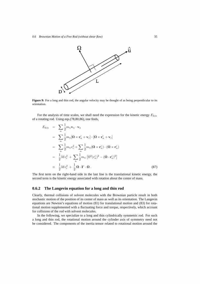
Figure 9: For a long and thin rod, the angular velocity may be thought ofas being perpendicular to itsorientation.
For the analysis of time scales, we shall need the expressionfor the kinetic energyEkin
of a rotating rod. Using eqs.(78,80,86), one finds,
Ekin =∑
n
1
2mnvn · vn
=∑
n
1
2mn[Ω× rc
n + vc] · [Ω× rcn + vc]
=∑
n
1
2mnv2
c +∑
n
1
2mn(Ω × rc
n) · (Ω× rcn)
=1
2Mv2
c +∑
n
1
2mn
[
Ω2(rcn)2 − (Ω · rc
n)2]
≡ 1
2Mv2
c +1
2Ω · Ic · Ω . (87)
The first term on the right-hand side in the last line is the translational kinetic energy, thesecond term is the kinetic energy associated with rotation about the center of mass.
0.6.2 The Langevin equation for a long and thin rod
Clearly, thermal collisions of solvent molecules with the Brownian particle result in bothstochastic motion of the position of its center of mass as well as its orientation. The Langevinequations are Newton’s equations of motion (81) for translational motion and (83) for rota-tional motion supplemented with a fluctuating force and torque, respectively, which accountfor collisions of the rod with solvent molecules.
In the following, we specialize to a long and thin cylindrically symmetric rod. For sucha long and thin rod, the rotational motion around the cylinder axis of symmetry need notbe considered. The components of the inertia tensor relatedto rotational motion around the
36
long cylinder axis are very small in comparison to its remaining components, and may bedisregarded. The angular velocityΩ is therefore understood to denote the component of theangular velocity perpendicular to the cylinder axis of symmetry (see fig9). The componentΩ
of the angular velocity that changes the orientation of the rod is equal to,
Ω = u× du
dt. (88)
This can be seen as follows. By definition we have,
du
dt= Ω× u , (89)
Operating on both sides withu×, using thatu× (Ω× u) = (u · u)Ω− (u ·Ω)u, and notingthatu · u = 1 andu · Ω = 0, eq.(88) is recovered.
The force and torque of the solvent on the rod consists of two parts. Once the rods attaineda finite translational and rotational velocity, there is a systematic force equal to−Γf · p/M(see eq.(38)) and a systematic torque equal to−γrΩ (see eq.(48)) on the rod due to friction.The second part is the fluctuating force and torque discussedbefore. Denoting the fluctuatingforce byf and the fluctuating torque byT, the complete set of Langevin equations reads (weomit the superscripts “c ” in the following),
dp/dt = −Γf
M· p + f(t),
dr/dt = p/M,
dJ/dt = −γr Ω + T(t),
I · Ω = J. (90)
Since systematic interactions with the solvent molecules are made explicit through frictioncontributions, the ensemble average of the fluctuating force and torque are zero,
< f(t) > = 0 ,
< T(t) > = 0 . (91)
Due to the fore mentioned large separation in time scales on which the solvent molecules relaxand the rod moves, it is sufficient for the calculation of the thermal movement of the Brownianparticle to use a delta correlated fluctuating force and torque in time, that is,
< f(t)f(t′) > = Gtrans δ(t − t′) ,
< T(t)T(t′) > = Grot δ(t − t′) , (92)
whereδ is the delta distribution andGtrans andGrot are constant3 × 3-dimensional ten-sors (where the subscripts stand for “translation” and “rotation”), which may be regarded asa measure for the strength of the fluctuating force and torque. They are referred to as thetranslational and rotational fluctuation strength, respectively. Such delta correlations limitthe description to a time resolution which is large with respect to the solvent time scale of10−13s.
Note that for the rods with a large aspect ratioL/D considered here, the inertia tensor ineq.(86) is easily calculated, replacing the sum over molecules by an integral. For a constant

0.6 Brownian Motion of a Free Rod (without shear flow) 37
local mass densityρ of the rod material, the inertia tensor becomes,
I =
∫
dr′ ρ [r′ 2I − r′r′] ≈ π
(
D
2
)2
ρ
∫ 12L
− 12L
dl l2 [I− uu] =1
12ML2 [I − uu] . (93)
The typical magnitude for the inertia tensor is thus112ML2. Note that sinceΩ is perpendicular
to u (see eq.(88)), it follows from eq.(93) that,
I ·Ω = 112
ML2 Ω . (94)
This result will be convenient in our further analysis of theLangevin equation.
0.6.3 The Brownian time scale :Relaxation rates of the translational and rotational velocity
The Langevin equation (90) can be used to estimate the time scale on which the translationaland rotational velocity decay to equilibrium with the heat bath of solvent molecules. Firstconsider the translational velocity. Ensemble averaging the first equation in (90), using eq.(92)gives,
d <p>
dt= − <
Γf
M· p > . (95)
Remember that the friction tensorΓf depends on the orientation of the rod, and can thereforenot be taken outside the ensemble averaging brackets< · · · >. However, the interest hereis in anestimateof the relaxation time of the translational velocity. Sincethe magnitude ofthe friction coefficient of a rod varies only a factor of two depending on its orientation, onecan use a typical magnitude of the elements ofΓf in eq.(95). This typical magnitude followsfrom the expression in eq.(38) as2πη0L/ lnL/D. The time scale on which the translationalvelocity relaxes can thus be estimated from,
d <p>
dt≈ − 2 π η0 L
M lnL/D <p> . (96)
It follows that (withp(0) the initial translational momentum),
<p> (t) ≈ p(0) exp −t/τtrans , with τtrans =M lnL/D
2 π η0 L≈ 1 ns . (97)
A typical value for the relaxation timeτtrans of the translational velocity of a rod is thus foundto be of the order of a nano second.
The time scale on which rotational velocities relax can be estimated from the last two ofthe equations in (90). Ensemble averaging gives, using eq.(91),
d <J>
dt= −γr <Ω> ,
<I · Ω> = <J> . (98)
Using eq.(94) in the second equation, and substitution of the result into the first equation leadsto,
d <Ω>
dt= − 12 γr
M L2<Ω> , (99)
38
and hence (withΩ(0) the initial angular velocity),
<Ω> (t) = Ω(0) exp −t/τrot , with τrot =12 M L2
γr=
M lnL/D4 π η0 L
≈ 1 ns. (100)
where the expression (49) for the rotational friction coefficient has been used. Relaxationtimes for translational and rotational velocities are thusboth of the order of a nano second.
Within a description where time is coarse grained to a time much larger thanτtrans andτrot, inertial forces and torques on the rod can be neglected. This will turn out to be animportant fact in further theoretical developments discussed later in this chapter. The corre-sponding coarsening in length scale and orientational angle will be discussed in the followingsection. The time scale that is much larger thanτtrans andτrot, but still small enough toresolve position and orientation in sufficient detail, is referred to asthe Brownian or diffusivetime scale.
0.6.4 The Brownian length scale and Brownian angle
As discussed in the beginning of this section, a coarsening in time implies a coarsening ofposition and angular orientation. On the Brownian time scale the spatial and angular resolutionis not better than the distance over which the Brownian particle moves and the angle overwhich a rod typically rotates, respectively, during a time interval equal to the Brownian timescale.
Consider first the length∆l that the rod traverses during the timeτ ≫ τtrans. This so-calledBrownian length scaleis easily obtained by integration of eqs.(97),
∆l =
∫ τ
0
dt|<p(t)>|
M=
|p(0) |M
τtrans (1 − exp−τ/τtrans) ≈ |p(0) |M
τtrans . (101)
A typical value for| p(0) | is obtained from the equipartition theorem,
|p(0) | ≈√
<|p | 2> =√
3MkBT . (102)
The Brownian length scale is thus estimated as,
∆l ≈√
3 M kB TlnL/D2 π η0 L
. (103)
Using typical numerical values for the several quantities gives,
∆l
L≈ 10−4 − 10−3 . (104)
The conclusion is that displacements that are very small in comparison to the length of the rodare still resolved on the Brownian time scale. When∆L/L would have been a large number, itwould have made no sense to coarsen to the Brownian time scale, since it is then not possibleto accurately describe the motion of the rod.
Next consider the typical angle∆Θ over which a rod rotates during a timeτ ≫ τrot. Thisis the so-calledBrownian angle. Integration of eq.(100) gives,
∆Θ =
∫ τ
0
dt |<Ω(t)>|= |Ω(0) | τrot (1 − exp−τ/τrot) ≈ |Ω(0) | τrot . (105)

0.6 Brownian Motion of a Free Rod (without shear flow) 39
According to eq.(94), the rotational contribution to the kinetic energy in eq.(87) is equal to124
ML2 |Ω |2. Hence, according to the equipartition theorem, a typical value for|Ω0 | can beestimated as,
|Ω(0) | ≈√
<|Ω |2> = 6
√
kB T
M L2. (106)
The Brownian angle is thus of the order,
∆Θ ≈ 6√
M kB TlnL/D4 π η0 L2
. (107)
For typical numerical values we have (note that, according to eq.(103), the right-hand side isequal to
√3 ∆L/L),
∆Θ
π≈ 10−4 − 10−3 . (108)
Very small angular displacements can thus still be resolvedon the Brownian time scale.For the study of processes where a significant translationaland rotational displacement
of the Brownian particle is essential, a statistical description on the Brownian time scale istherefore sufficient.
0.6.5 Calculation of fluctuation strengths
Analyzing the Langevin equation requires the determination of the fluctuation strengths ineq.(92). This can be done using the equipartition theorem for translational and rotationalmotion, after having solved the Langevin equation forp(t) andΩ(t).
First consider the translational velocity. Integration ofthe first equation of motion in (90)yields,
p(t) = exp
−Γf
Mt
· p(0) +
∫ t
0
dt′ exp
−Γf
M(t − t′)
· f(t′) . (109)
The exponent of a tensor,A say, is defined through the Taylor expansion,
expA ≡∞∑
n=0
1
n!An , (110)
whereAn is A · A · · ·A, n times, andA0 ≡ I, the identity tensor. Now, from eq.(43) it iseasily shown by induction that,
Γnf = γn
‖ uu + γn⊥ [ I − uu ] , (111)
and hence, from the defining expression (110) for the tensor exponential,
exp
−Γf
M(t − t′)
= exp
− γ‖
M(t − t′)
uu + exp
−γ⊥M
(t − t′)
[I − uu] . (112)
Equation (109) can thus be written as,
p(t) = p‖(t) + p⊥(t) , with p‖ ≡ uu · p , andp⊥ ≡ [ I− uu ] · p , (113)
40
with,
p‖(t) ≡ exp
− γ‖
Mt
p‖(0) +
∫ t
0
dt′ exp
− γ‖
M(t − t′)
f‖(t′) ,
p⊥(t) ≡ exp
−γ⊥M
t
p⊥(0)+
∫ t
0
dt′ exp
−γ⊥M
(t − t′)
f⊥(t′) , (114)
where the components of the random force parallel and perpendicular to the rods orientationare respectively defined as,
f‖(t) ≡ u(t)u(t) · f(t) , and f⊥(t) ≡ [ I − u(t)u(t) ] · f(t) . (115)
Instead of using the full tensor form in eq.(95) for the fluctuating force, we shall only needcorrelation functions of inner products of its two componentsf‖ andf⊥. Sincef(t) varies withtime much faster thanu(t), the latter is virtually constant over time intervals equalto manytimes the correlation time of the former. The conditional ensemble averages off‖,⊥, with aprescribedu, are therefore still0, and their correlation functions are still delta correlated on atime scale much larger than the solvent time scale. For the same reason,
< f‖(t) · f⊥(t′) > = 0 . (116)
We shall therefore define two independent fluctuation strengths for the fluctuating force par-allel and perpendicular to the rods orientation,
< f‖(t) · f‖(t′) > = G‖ δ(t − t′),
< f⊥(t) · f⊥(t′) > = G⊥ δ(t − t′). (117)
Notice that we are working here with inner products instead of dyadic products as for thespherical particle, so that bothG‖ andG⊥ are scalars. Since< p‖(t) · p⊥(t) >= 0, thekinetic energy corresponding to translational motion of the Brownian rod is a sum of twoquadratic terms related to the perpendicular velocity and asingle quadratic term related to theparallel velocity. From the equipartition theorem it is thus found that,
limt→∞
< p‖(t) · p‖(t) > = M/β,
limt→∞
< p⊥(t) · p⊥(t) > = 2 M/β. (118)
Substitution of eq.(114) into the above expressions, usingeqs.(116,117), it is readily foundthat,
G‖ = 2γ‖/β ,
G⊥ = 4γ⊥/β . (119)
This concludes the determination of the translational fluctuation strengths, which will be usedto investigate the translational Brownian motion of the rodin the following section.
Next consider the fluctuation strength for the correlation function in eq.(92) of the torque.Using eq.(94) in the last equation in (90), substituting theresult into the third equation andintegration yields,
Ω(t) = Ω(0) exp
− 12γr
ML2t
+12
ML2
∫ t
0
dt′ T(t′) exp
− 12γr
ML2(t − t′)
. (120)

0.6 Brownian Motion of a Free Rod (without shear flow) 41
Using the second equation in (92) thus leads to,
limt→∞
< Ω(t)Ω(t) > =6
γrML2Gr. (121)
From eq.(87) for the kinetic energy together with eq.(94) and one finds that the kinetic energydue to rotational motion is equal to124ML2Ω2(t). The equipartition theorem implies that124
ML2Ω2(t) = 32kBT . Hence,
limt→∞
< Ω(t)Ω(t) > = 12 IkBT
ML2. (122)
Combining this with eq.(121) identifies the rotational fluctuation strength,
Gr = I2γr
β. (123)
This expression allows for the analysis of the rotational part of the Langevin equation.
0.6.6 Translational Brownian motion of a rod
The simplest quantity that characterizes translational Brownian motion is themean squareddisplacement, defined as,
W (t) ≡ <|r(t) − r(t = 0) |2> , (124)
where the brackets denote ensemble averaging. This quantity can be calculated from theLangevin equation as follows.
We shall calculate the mean squared displacement on the Brownian time scale. As men-tioned before, inertial forces can be neglected on the Brownian time scale. Neglecting theinertial forcedp/dt on the left hand-side of the first equation in (90) gives,
dr/dt = Γ−1f · f(t) , (125)
whereΓ−1f is the inverse ofΓf . The reason for neglecting the inertial force can be made more
explicit as follows. Lett′ = t/τ be the dimensionless time in units of the Brownian time scaleτ . Rescaling the first equation in eq.(90) gives,
τtrans
τ
dp
dt′= − τtrans
Γf
M· p + τtrans f(τ t′) . (126)
Since the typical magnitude of the elements of the tensorΓf/M is 1/τtrans (see eqs.(38,97)),so thatτtrans Γf/M is of order unity, andτ ≫ τtrans on the Brownian time scale, thisis a singularly perturbed differential equation. That is, the inertial term is important onlyover a very small time interval int′, which is the mathematical boundary layer connectedto the singular perturbation. During this time interval themomentum coordinate relaxes toequilibrium with the solvent. Beyond this small time interval, wheredp/dt′ is not very largeanymore, so that the inertial contribution can be neglected. This immediately leads to eq.(125).
The inverse of the friction tensor appearing in eq.(125) is easily calculated,
Γ−1f =
1
γ‖uu +
1
γ⊥[ I− uu ] . (127)

42
The Langevin equation can thus be written in terms of the parallel and perpendicular compo-nents of the random force (see eq.(115)),
dr/dt =1
γ‖f‖(t) +
1
γ⊥f⊥(t) , (128)
hence,
r(t) = r(t = 0) +
∫ t
0
dt′[
1
γ‖f‖(t
′) +1
γ⊥f⊥(t′)
]
. (129)
Using that the fluctuating forces are delta correlated with fluctuation strengths given in eq.(119),one readily finds that,
W (t) = 6 D t , (130)
where,
D =1
3
(
D‖ + 2D⊥
)
. (131)
Here we introduced the Einstein translational diffusion coefficients for parallel and perpendic-ular motion,
D‖ = kBT/γ‖ ,
D⊥ = kBT/γ⊥ . (132)
For timest ≪ τtrans, where friction with the solvent has not been effective, thevelocity ofthe center of mass of a rod is constant. The mean squared displacement then varies like∼ t2.On the Brownian time scale, that is for timest ≫ τtrans, many independent collisions of therod with solvent molecules have occurred. This apparently leads to a linear variation ofW (t)with time. Such dynamic behaviour is calleddiffusive.
0.6.7 Orientational correlations
The simplest quantity that characterizes rotational Brownian motion is therotational meansquared displacement,
Wrot(t) ≡ <| u(t) − u(t = 0) |2> = 2 [ 1− < u(t) > · u(t = 0) ] . (133)
This rotational displacement is calculated on the Browniantime scale. For the same reason asfor translational motion, the inertial term for the rotational langevin equation of motion canbe neglected on the Brownian time scale. The third of the equations of motion in (90) thusreduces to,
Ω = u× du
dt=
1
γrT(t) . (134)
where eqs.(88,94) have been used. As a first step to obtain an expression for the rotationalmean squared displacement (133), the differential equation (134) should be solved foru(t) interms of the fluctuating torqueT. To this end, eq.(134) is rewritten as,
du/dt =1
γrT(t) × u . (135)

0.6 Brownian Motion of a Free Rod (without shear flow) 43
t -t1 2
<T(t ) T(t )>1 2
O t -t1 2
t -t1 2
<T(t ) T(t )>1 2
<T(t ) T(t )>1 2
O
Figure 10: Integration of the correlation function of the torque over half the domain of its argument.
To integrate this equation, the right-hand side is written as a tensor multiplication,
du/dt = A(t) · u , (136)
with,
A(t) ≡ 1
γr
0 −T3(t) T2(t)T3(t) 0 −T1(t)−T2(t) T1(t) 0
, (137)
whereTj is the jth component ofT. The differential equation (136) is equivalent to theintegral equation,
u(t) = u(0) +
∫ t
0
dt′ A(t′) · u(t′) , (138)
which is solved by iteration,
u(t) = u(0) +
∞∑
n=1
∫ t
0
dt1
∫ t1
0
dt2
∫ t2
0
dt3 · · ·∫ tn−2
0
dtn−1
∫ tn−1
0
dtn
A(t1) ·A(t2) · · · · · A(tn) · u(0) . (139)
For the calculation of the ensemble average ofu(t), the ensemble averages of the multipleintegrals over products ofA’s must be evaluated explicitly. From the definition of the tensor
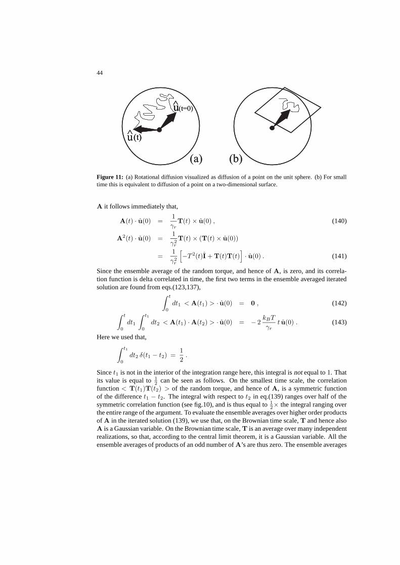
44
u(t=0)
(a) (b)
u(t)^
uu(t=0)
(a) (b)
u(t)u(t)^
Figure 11: (a) Rotational diffusion visualized as diffusion of a pointon the unit sphere. (b) For smalltime this is equivalent to diffusion of a point on a two-dimensional surface.
A it follows immediately that,
A(t) · u(0) =1
γrT(t) × u(0) , (140)
A2(t) · u(0) =1
γ2r
T(t) × (T(t) × u(0))
=1
γ2r
[
−T 2(t)I + T(t)T(t)]
· u(0) . (141)
Since the ensemble average of the random torque, and hence ofA, is zero, and its correla-tion function is delta correlated in time, the first two termsin the ensemble averaged iteratedsolution are found from eqs.(123,137),
∫ t
0
dt1 < A(t1) > · u(0) = 0 , (142)
∫ t
0
dt1
∫ t1
0
dt2 < A(t1) ·A(t2) > · u(0) = − 2kBT
γrt u(0) . (143)
Here we used that,∫ t1
0
dt2 δ(t1 − t2) =1
2.
Sincet1 is not in the interior of the integration range here, this integral isnotequal to1. Thatits value is equal to12 can be seen as follows. On the smallest time scale, the correlationfunction< T(t1)T(t2) > of the random torque, and hence ofA, is a symmetric functionof the differencet1 − t2. The integral with respect tot2 in eq.(139) ranges over half of thesymmetric correlation function (see fig.10), and is thus equal to 1
2× the integral ranging overthe entire range of the argument. To evaluate the ensemble averages over higher order productsof A in the iterated solution (139), we use that, on the Brownian time scale,T and hence alsoA is a Gaussian variable. On the Brownian time scale,T is an average over many independentrealizations, so that, according to the central limit theorem, it is a Gaussian variable. All theensemble averages of products of an odd number ofA’s are thus zero. The ensemble averages
0.6 Brownian Motion of a Free Rod (without shear flow) 45
of products of an even number ofA’s can be written as a sum of products of averages of onlytwo A’s. Consider for example the ensemble average of then = 4 term in the iterated solution(summation over the repeated indicesp, q, r, s is understood here,Aij is theijth componentof A andus(0) is thesth component ofu(0)),
∫ t
0
dt1
∫ t1
0
dt2
∫ t2
0
dt3
∫ t3
0
dt4 < Aip(t1)Apq(t2)Aqr(t3)Ars(t4) > us(0) =
∫ t
0
dt1
∫ t1
0
dt2
∫ t2
0
dt3
∫ t3
0
dt4 [ < Aip(t1)Apq(t2) >< Aqr(t3)Ars(t4) > us(0)
+ < Aip(t1)Aqr(t3) >< Apq(t2)Ars(t4) > us(0)
+ < Aip(t1)Ars(t4) >< Apq(t2)Aqr(t3) > us(0) ] .
For the respective products of ensemble averages in the above equation we need to evaluatethe following integrations over delta distributions,
∫ t
0
dt1
∫ t1
0
dt2
∫ t2
0
dt3
∫ t3
0
dt4 δ(t1 − t2) δ(t3 − t4) ,
∫ t
0
dt1
∫ t1
0
dt2
∫ t2
0
dt3
∫ t3
0
dt4 δ(t1 − t3) δ(t2 − t4) ,
and,∫ t
0
dt1
∫ t1
0
dt2
∫ t2
0
dt3
∫ t3
0
dt4 δ(t1 − t4) δ(t2 − t3) .
The first of these four-fold integrals is equal to,∫ t
0
dt1
∫ t1
0
dt2
∫ t2
0
dt3
∫ t3
0
dt4 δ(t1 − t2) δ(t3 − t4) =
(
1
2
)21
2t2 ,
where the factor(1/2)2 originates from integration of delta functions ranging over half thedomain of their arguments, as explained above. By inspection, the other two four-fold integralsturn out to be zero, because the arguments of the delta functions are non-zero in the entireintegration range. Only products with the consecutive timeorderingt1 → t2 → t3 → · · · →tn contribute. Using the expression (123) for the rotational fluctuation strength, we thus arriveat the following result,
∫ t
0
dt1
∫ t1
0
dt2
∫ t2
0
dt3
∫ t3
0
dt4 < A(t1) · A(t2) · A(t3) ·A(t4) > · u(0)
=
(
− 4
βγr
)2 (
1
2
)21
2t2 u(0) .
In the next higher order terms in the ensemble average of the iterative solution (139), theproduct with the consecutive time ordering is likewise the only surviving one. Along similarlines one shows that, for evenn’s,
∫ t
0
dt1 · · ·∫ tn−1
0
dtn < A(t1) · · · · · A(tn) >=
(
− 4
βγr
)n/2 (
1
2
)n/21n2 !
tn/2 I .

46
The iterative solution is thus,
< u(t) > =
[
∞∑
n=0
1
n!(−2Dr)
n tn
]
u(0) = exp−2Drt u(0) , (144)
where therotational diffusion coefficientDr is defined by the Einstein relation,
Dr = kBT/γr . (145)
Therotational mean squared displacementis thus equal to,
Wrot(t) = 2 [ 1 − exp−2Drt ] . (146)
For small times this result is quite similar to eq.(130) for the mean squared displacement ofthe center of mass of a rod,
Wrot(t) = <| u(t) − u(t = 0) |2> = 4 Dr t , Dr t ≪ 1 . (147)
This corresponds to diffusion of a point in two dimensions. Rotational Brownian motion maybe visualized as a point on the unit spherical surface, representing the tip of the unit vectoru, which exerts Brownian motion (see fig.11a). For small timesthis is Brownian motion on atwo dimensional flat surface (see fig.11b). For larger times the tip experiences the curvatureof the unit spherical surface, leading to the more complex behaviour as described by eq.(146).
0.7 Equations of Motion for Interacting Rods
So far, we have considered rods which do not interact with other rods. For systems of in-teracting rods, properties are most easily studied by meansof probability density functions(pdf’s) of positions and orientations. In this section we shall derive the fundamental equationof motion for the probability density function of the positions and orientations of an assemblyof N interacting rods. This equation of motion is commonly referred to asthe Smoluchowskiequation. An essential ingredient in the derivation of this equationof motion is the neglectof inertia on the Brownian time scale, as discussed before. The Smoluchowski equation alsodescribes the dynamics of non-interacting rods, and is shown to reproduce results obtained inprevious sections. In addition, the behaviour of non-interacting rods in shear flow is discussedat the end of this section.
0.7.1 The N-particle Smoluchowski equation
Consider a single cylindrically symmetric, rigid rod embedded in solvent. The position coor-dinate of the rod will be denoted byr, while its orientation is characterized by the unit vectoru which is directed along the long axis of the rod. The “microstate” of the rod is thus set bya point inℜ3 (the position vectorr) and a point on the unit spherical surface (the tip of thevectoru), as depicted in fig.12. The points inℜ3 and on the unit spherical surface exhibitchaotic motion due to translational- and rotational Brownian motion, respectively. Considernow an ensemble ofN containers, where each container is filled with solvent and contains
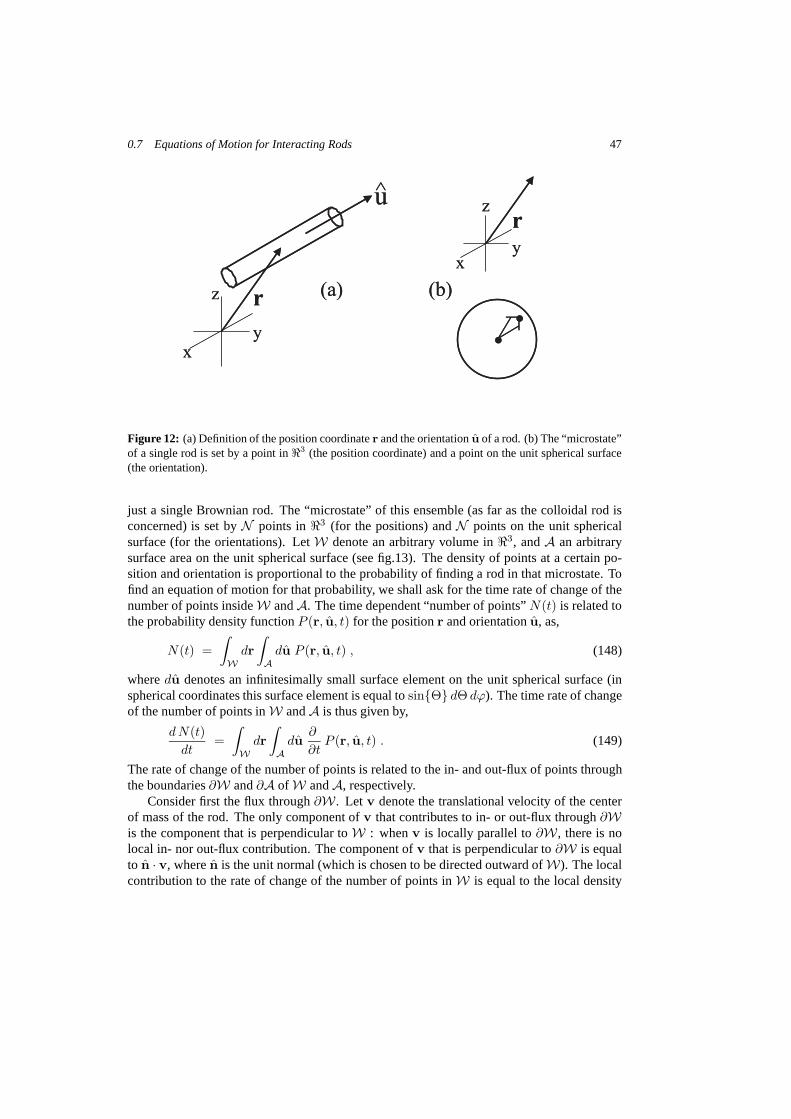
0.7 Equations of Motion for Interacting Rods 47
u
xy
z r (a)
xy
zr
·
·
(b)
u
xy
z r (a)
xy
zr
·
·
(b)
Figure 12: (a) Definition of the position coordinater and the orientationu of a rod. (b) The “microstate”of a single rod is set by a point inℜ3 (the position coordinate) and a point on the unit spherical surface(the orientation).
just a single Brownian rod. The “microstate” of this ensemble (as far as the colloidal rod isconcerned) is set byN points inℜ3 (for the positions) andN points on the unit sphericalsurface (for the orientations). LetW denote an arbitrary volume inℜ3, andA an arbitrarysurface area on the unit spherical surface (see fig.13). The density of points at a certain po-sition and orientation is proportional to the probability of finding a rod in that microstate. Tofind an equation of motion for that probability, we shall ask for the time rate of change of thenumber of points insideW andA. The time dependent “number of points”N(t) is related tothe probability density functionP (r, u, t) for the positionr and orientationu, as,
N(t) =
∫
W
dr
∫
A
du P (r, u, t) , (148)
wheredu denotes an infinitesimally small surface element on the unitspherical surface (inspherical coordinates this surface element is equal tosinΘ dΘ dϕ). The time rate of changeof the number of points inW andA is thus given by,
dN(t)
dt=
∫
W
dr
∫
A
du∂
∂tP (r, u, t) . (149)
The rate of change of the number of points is related to the in-and out-flux of points throughthe boundaries∂W and∂A of W andA, respectively.
Consider first the flux through∂W . Let v denote the translational velocity of the centerof mass of the rod. The only component ofv that contributes to in- or out-flux through∂Wis the component that is perpendicular toW : whenv is locally parallel to∂W , there is nolocal in- nor out-flux contribution. The component ofv that is perpendicular to∂W is equalto n · v, wheren is the unit normal (which is chosen to be directed outward ofW). The localcontribution to the rate of change of the number of points inW is equal to the local density

48
x
y
z
W A
Figure 13: The “microstate” of the ensemble is given by a point distribution in ℜ3 and on the unitspherical surface.W andA are arbitrary subspaces inℜ3 and on the unit spherical surface, respectively.
of pointsP (r, u, t), multiplied by the perpendicular componentn · v of v. The total rateof changedNW(t)/dt of the number of points due to in- and out-flux through∂W is thusequal to (withdS = ndS, wheredS is an infinitesimally small surface element on∂W ; seefig.14a),
dNW(t)
dt= −
∮
∂W
dS ·∫
A
du [v P (r, u, t) ] . (150)
The minus sign here is due to the fact that the direction ofn is pointing outward ofW : whenv ∼ n, so thatn·v > 0, the number points inW decreases in time. ApplyingGauss’s integraltheoremit is found that,
dNW(t)
dt= −
∫
W
dr
∫
A
du∇ · [vP (r, u, t) ] . (151)
Next consider the contributiondNA(t)/dt of the rate of change due to in- and out-fluxthrough the boundary∂A of A. This boundary is a closed curve on the unit spherical sur-face. Sinceu is always perpendicular to the unit spherical surface, the vector that is locallyperpendicular to∂A is equal todl × u, wheredl is the infinitesimally small vector that islocally tangential to the curve∂A (see fig.14b). The component of the velocitydu/dt that isperpendicular to∂A is thus equal to(dl× u) ·du/dt, which is the component that determinesthe in- and out-flux. Since this is equal todl · (u×du/dt), the total rate of changedNA(t)/dtof the number of points inA is thus equal to,
dNA(t)
dt= −
∫
W
dr
∮
∂A
dl ·(
u× du
dt
)
P (r, u, t) . (152)
Applying Stokes’s integral theorem, it is found that,
dNA(t)
dt= −
∫
W
dr
∫
A
du u ·
∇u ×(
u × du
dt
)
P (r, u, t)
, (153)
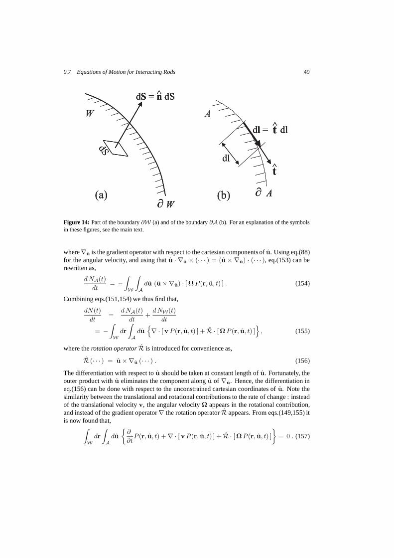
0.7 Equations of Motion for Interacting Rods 49
W
W
dS = n dS^
(a)
A
A
t^
dl = dlt^
dl
dS
(b)
W
W¶ W
dS = n dS^dS = n dS^
(a)
A
A¶ A
t^t^
dl = dlt^dl = dlt^t^
dl
dS
(b)
Figure 14: Part of the boundary∂W (a) and of the boundary∂A (b). For an explanation of the symbolsin these figures, see the main text.
where∇u is the gradient operator with respect to the cartesian components ofu. Using eq.(88)for the angular velocity, and using thatu · ∇u × (· · · ) = (u × ∇u) · (· · · ), eq.(153) can berewritten as,
dNA(t)
dt= −
∫
W
∫
A
du (u ×∇u) · [ΩP (r, u, t) ] . (154)
Combining eqs.(151,154) we thus find that,
dN(t)
dt=
dNA(t)
dt+
dNW(t)
dt
= −∫
W
dr
∫
A
du
∇ · [v P (r, u, t) ] + R · [ΩP (r, u, t) ]
, (155)
where therotation operatorR is introduced for convenience as,
R (· · · ) = u×∇u (· · · ) . (156)
The differentiation with respect tou should be taken at constant length ofu. Fortunately, theouter product withu eliminates the component alongu of ∇u. Hence, the differentiation ineq.(156) can be done with respect to the unconstrained cartesian coordinates ofu. Note thesimilarity between the translational and rotational contributions to the rate of change : insteadof the translational velocityv, the angular velocityΩ appears in the rotational contribution,and instead of the gradient operator∇ the rotation operatorR appears. From eqs.(149,155) itis now found that,
∫
W
dr
∫
A
du
∂
∂tP (r, u, t) + ∇ · [vP (r, u, t) ] + R · [ΩP (r, u, t) ]
= 0 . (157)

50
Since this holds for arbitrary volumesW and surface areasA, the integrand must be equal to0. Hence,
∂
∂tP (r, u, t) = −∇ · [v P (r, u, t) ] − R · [ΩP (r, u, t) ] . (158)
Here, we considered a system that contained just a single rod. For a suspension that containsN rods, instead of justr, u, the relevant phase space coordinates are,
r1, r2, · · · , rN , u1, u2, · · · , uN ,
whererj is the position of thejth rod, anduj its orientation. The equation of motion forthe probability density functionP of these phase space coordinates is found from eq.(158) bysimply adding the in- and out-fluxes over all rods,
∂
∂tP (r1, · · · , rN , u1, · · · , uN , t) = −
N∑
j=1
∇j · [vj P ] + Rj · [Ωj P ]
. (159)
The full phase space coordinate dependence ofP is not denoted here on the right-hand sidefor brevity. Here,Rj is defined as in eq.(156), withu is replaced byuj . This is an exactresult, since it merely expresses conservation of the number of rods.
As a last step, the translational- and rotational velocities have to be expressed in termsof functions of the phase space coordinates. In doing so, we shall neglect hydrodynamicinteractions between the rods. The reason for this neglect is two-fold. First of all, as will beseen later, the volume fractions of interest scale asD/L (with D the thickness andL the lengthof the rods). That is, the volume fraction where the isotropic-nematic phase transition occursscales asD/L. For the study of dynamics in the isotropic phase and the isotropic-nematicphase transition, volume fractions are thus very low. This implies that on average two arbitrarysurface elements of distinct rods are very far apart. Therefore, hydrodynamic interactions areprobably much less important than for suspensions of spherical particles. Secondly, the preciseform of hydrodynamic interaction functions for rods is unknown, even on the two-body level.
The key relation to express the velocities in terms of phase functions is the force balanceequation. As has been seen before, translational and angular momentum coordinates are re-laxed to equilibrium with the heat bath of solvent moleculeson the Brownian time scale, sothat the total force (and torque) on each Brownian particle is zero. There are three non-inertialforces (and torques) working on each rod : the hydrodynamic forceFh
j (torqueThj ) that the
solvent exerts on the rod, the direct interaction forceFIj (torqueTI
j ) and the Brownian forceFBr
j (torqueTBrj ), which will be discussed and specified later. Hence,
Total force = 0 = Fhj + FI
j + FBrj ,
Total torque = 0 = Thj + TI
j + TBrj . (160)
The direct force is minus the gradient of the total potentialenergyΦ of the assembly of Brow-nian particles,
FIj = −∇j Φ(r1, · · · , rN , u1, · · · , uN ) , (161)
while the direct torque is related toΦ as,
TIj = −RjΦ . (162)
0.7 Equations of Motion for Interacting Rods 51
With the neglect of hydrodynamic interactions, the hydrodynamic torque and force are justthe friction forces of a single rod with the solvent. This friction force is equal to (see eq.(44)),
Fhj =
(
γ‖uu + γ⊥
[
I− uu])
· (vc − G · rc) . (163)
The torque due to friction with the solvent is equal to (see eq.(48)),
T hj = −γr [Ωj − uj × G · uj ] . (164)
As discussed before, in case of simple shear flow, the second term in the square brackets is0 when the rod’s orientation is along the flow direction. To correctly describe Jeffery orbitsof non-Brownian rods we therefore had to add the small torquethat acts on rods with such anorientation (see eq.(55)). For Brownian rods this small torque is irrelevant, since rods orientedparallel to the flow direction will attain other orientations due to Brownian motion before thementioned small torque became active.
The translational velocity can be found from eqs.(160,163)as,
vj =(
D‖ujuj + D⊥
[
I − ujuj
])
·
−β∇jΦ + βFBrj
+ γ G · rj , (165)
while the rotational velocity is found from eqs.(160,164) as,
Ωj = Dr
−βRjΦ + βTBrj
+ γ uj ×(
G · uj
)
. (166)
Here,G = G/γ is the “normalized” velocity gradient tensor,
D‖ = kBT/γ‖ , D⊥ = kBT/γ⊥ . (167)
are the translational diffusion coefficients for motion parallel and perpendicular to the rodslong axis, respectively, and,
Dr = kBT/γr , (168)
is the rotational diffusion coefficient. These diffusion coefficients depend on the lengthL andthicknessD of the rod, and the shear viscosityη0 of the solvent (see eqs.(40,42,49)),
Dr =3kBT lnL/D
π η0 L3
D‖ =kBT lnL/D
2π η0 L, (169)
D⊥ = 12D‖ .
Note that due to the last two equations here, eq.(165) can be rewritten as,
vj = 34D
[
I + ujuj
]
·
−β∇jΦ + βFBrj
+ γ G · rj , (170)
wherethe translational diffusion coefficientD is equal to,
D = 13
[
D‖ + 2D⊥
]
= 43D⊥ = 2
3D‖ =
kBT lnL/D3π η0 L
. (171)
The reason for referring toDr andD as “diffusion coefficients” will become clear in the fol-lowing section, where diffusion of non-interacting rods isconsidered. The above expressions
52
for diffusion coefficients are valid for very long and thin rods. For shorter rods, corrections tothese limiting expressions are given by de la Torre and Bloomfield (1981).
We still have to express the Brownian contributions to the total force and torque in terms ofphase functions. This is achieved as follows. In the absenceof flow, for infinite timet → ∞,when the suspension attains equilibrium, the probability density functionP is proportionalto the Boltzmann exponentialexp−β Φ, and∂P/∂t = 0. From the long-time limit ofeq.(159), together with eqs.(166,170) in the absence of shear flow, it follows that,
FBrj = −kBT∇j lnP ,
TBrj = −kBT Rj lnP . (172)
These Brownian contributions to the total force and torque are the result of the fact that theforce balance equations (160) are only valid on the diffusive time scale. On such a coars-ened time scale, not only the purely microscopic forcesFh
j andFIj (and the corresponding
torques) act on the colloidal particles. The additional Brownian force (and torque) arises frominteractions of the colloidal particle with the solvent molecules, averaged with respect to theequilibrium probability density function for the phase space coordinates of the fluid moleculesin the external field imposed by the colloidal particles withprescribed positions and orienta-tions. Even in a very dilute system of colloidal particles (an “ideal gas”), where interactionsbetween the colloidal particles can be neglected, the equilibrium state is one where the macro-scopic density is constant, independent of position. The forces that drive such an ideal gas tothe homogeneous state are the Brownian forces.
In this way the following equation of motion for the probability density functionP of thephase space coordinatesr1, · · · , rN , u1, · · · , uN is obtained,
∂P
∂t=
N∑
j=1
34D∇j ·
(
I + ujuj
)
· [∇jP + β P∇jΦ] − γ ∇j ·[
P G · rj
]
+ DrRj ·[
RjP + β P RjΦ]
− γ Rj ·[
P uj ×(
G · uj
)]
. (173)
This is theSmoluchowski equationfor very long and thin, rigid rods, where hydrodynamicinteractions are neglected.
An alternative, perhaps more satisfying derivation of the Smoluchowski equation, is tostart from the Liouville equation for a binary mixture : the solvent molecules and the colloidalparticles. The Smoluchowski equation is then found after integrating over the fast phase spacevariables (the phase space coordinates of the solvent molecules and the momentum coordi-nates of the colloidal particles). Such an approach has beentaken, for spherical colloids, byDeutch and Oppenheim (1971) and Murphy and Aquirre (1972). The Smoluchowski equationfor spherical particles has been used as a starting point to derive the Smoluchowski equationfor rods by Erpenbeck and Kirkwood (1963).
0.7.2 Translational and rotational diffusion of non-interactingrods without shear flow
Consider the mean squared center of mass displacement of a freely diffusing rod. Its positionat timet = 0 will be chosen at the origin :r(t = 0) = 0. Free diffusion occurs in suspensions
0.7 Equations of Motion for Interacting Rods 53
where the concentration of colloidal particles is so small,that on average, rods do not noticeeach other. In that case, the interaction potential in the Smoluchowski equation (173) may beneglected (Φ = 0), andN can be taken equal to1, resulting in,
∂
∂tP (r, u, t) = 3
4D∇ ·
[
I + uu]
· ∇P + DrR2P , (174)
whereR2= R · R. For the highly diluted systems under consideration each orientation
has equal probability,P (r, u, t) is independent ofu, and is simply proportional toP (r, t).Equation 174 thus reduces to,
∂
∂tP (r, t) = 3
4D∇ ·
[
I + uu]
· ∇P (r, t) . (175)
Integration of both sides with respect tou, using that,1∮
du[
I + uu]
= 43I ,
thus leads to,
∂
∂tP (r, t) = D∇2P (r, t) . (176)
The equation of motion for the dyadic product< r(t)r(t) > is obtained by multiplying bothsides withr r and integrating,
d
dt
∫
dr r r P (r, t) ≡ d
dt< r(t)r(t) > = D
∫
dr rr∇2P (r, t)
= D
∫
drP (r, t)∇2rr = 2D I ,
where Gauss’s integral theorem has been used twice in the second line. Since<r(t = 0)r(t =0)>= 0, time-integration immediately leads to,
< r(t)r(t) > = 2Dt I ,
and hence,
W (t) ≡ < r2(t) > = 6Dt , (177)
in accordance with the result (130) as obtained from the Langevin equation. Note that ontaking the Trace of the dyadic product, each spatial dimension (3 in this case) gives rise to afactor 2 on the right-hand side in the mean squared displacement in eq.(177). Diffusion in twodimensions gives a prefactor of4 instead of6, in accordance with the result in eq.(147) forshort-time rotational diffusion.
Let us now consider the time dependence of the orientation< u(t) >, given thatu(t =0) = u(0). For a homogeneous system,P (r, u, t) is independent ofr, so that eq.(174) reducesto,
∂
∂tP (u, t) = Dr R
2P (u, t) . (178)
1 The integralH
du (· · · ) stands for integration over the unit spherical surface. In terms of the angular spherical
coordinatesΘ andϕ of u this integral isR π0 dΘ
R 2π0 dϕ sinΘ (· · · ).

54
Multiplying both sides withu and integrating over the unit spherical surface gives,
d
dt< u(t) > = Dr
∮
du u R2 P (u, t) .
From Stokes’s integral theorem it follows that for any two (well behaved) functionsf andgof u,
∮
du f(u)Rg(u) = −∮
du g(u)Rf(u) . (179)
Applying this result twice leads to,∮
du uR2 P (u, t) =
∮
duP (u, t)R2 u = −2 < u(t) > ,
where it is used thatR2u = −2u. The equation of motion we were after thus reads,
d
dt< u(t) > = −2Dr < u(t) > ,
the solution of which is,
< u(t) > = exp−2Drt u(0) . (180)
in accordance with eqs.(133,146) as obtained from the Langevin equation. As discussed in thesection on the Langevin-equation approach, for small timeswhereDrt ≪ 1, this result canbe interpreted as translational diffusion of the tip ofu on a two-dimensional surface.
0.8 The Orientational Order Parameter
At higher concentrations, where interactions between rodsare important, a transition from anisotropic distribution of orientations to an orientationally ordered nematic state can occur (aswill be discussed in more detail later). Orientational order is also induced by shear flow inotherwise isotropic suspensions. For such ordered states the degree of orientational ordervaries, depending on the concentration of rods and the shearrate. In the present sectionthe so-calledorientational order parameterwill be defined, which measures the degree oforientational order.
u
Q
n
Figure 15: Definition of the angleΘ between the orientationu of a rod and the directorn.
0.8 The Orientational Order Parameter 55
The preferred orientationn of the rods is referred to asthe director. The most simplemeasure for the degree of orientation that comes to mind is<cosΘ>=< u > ·n, whereΘis the angle of the orientationu of a given rod and the directorn (see fig.15). However, due tosymmetry, an orientationu is equally likely to occur as the orientation−u, so that< u >= 0.The next most simple measure would then be< cos2Θ >=< uu >: nn. 2. Hence, themost simple quantity that characterizes the orientationalstate is the so-calledorientationalorder parameter tensor,
S ≡ < u u > ≡∮
du u u P (u) , (181)
where the integration ranges over the unit spherical surface (see 1). Furthermore,P (u) isthe probability density function (pdf) for the orientationu of a rod, which can in principle beobtained from the solution of theN -particle Smoluchowski equation (173), noting that,
P (u) =
∫
dr1 · · ·∫
drN
∮
du2 · · ·∮
duN P (r1, · · · , rN , u, u2, · · · , uN ) . (182)
The pdf ofu can be time dependent, in which case orientational dynamicscan be studied.What information can be distilled from a specifiedS ? To answer this question, lete be a
unit vector, and letϕ denote the angle between the orientationu of a given rod ande. Considerthe function,
f ≡ < cos2ϕ > = S : ee =∑
m,n
Smn em en , (183)
whereSnm is thenmth component ofS, anden thenth component ofe. Since the maximumvalue ofcos2ϕ is attained whenϕ = 0, and the most likely direction ofu is along thedirector, it is evident that the unit vectore that maximizesf is the director. Maximization off has to be performed under the constraint thate is a unit vector, that ise · e = 1. Accordingto Lagrange’s principle, we therefore have to maximize the function,
f∗ = f − λ e · e =∑
mn
Smn − λ δmn em en , (184)
whereλ is the Lagrange multiplier, andδnm is the Kronecker delta (δmn = 0 whenm 6= nandδmn = 1 whenm = n). From∂f/∂em = 0 it is easily found that,
S · e = λ e , maximizes or minimizesf∗ . (185)
By taking the inner product on both sides it follows that,
λ = S : ee , whene maximizes or minimizesf∗ . (186)
We thus find that,
The eigenvector ofS with the largest eigenvalue is the directorn and the largest eigen-value is equal to<cosΘ2 >= S : nn.
2 The contraction symbol “: ” stands for summation over two adjacent indices, that is, for two tensorsA andB,by definition,A : B =
P
n,m AnmBmn
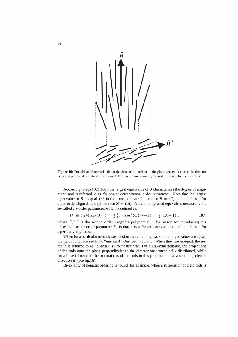
56
n
ˆ 'n
Figure 16: For a bi-axial nematic, the projections of the rods onto the plane perpendicular to the directorn have a preferred orientationn′ as well. For a uni-axial nematic, the order in this plane is isotropic.
According to eqs.(183,186), the largest eigenvalue ofS characterizes the degree of align-ment, and is referred to asthe scalar orientational order parameter. Note that the largesteigenvalue ofS is equal1/3 in the isotropic state (since thenS = 1
3I), and equal to1 for
a perfectly aligned state (since thenS = nn). A commonly used equivalent measure is theso-calledP2-order parameter, which is defined as,
P2 ≡< P2(cosΘ) > = 12
3 <cos2Θ> −1
= 123λ − 1 , (187)
whereP2(x) is the second order Legendre polynomial. The reason for introducing this“rescaled” scalar order parameterP2 is that it is0 for an isotropic state and equal to1 fora perfectly aligned state.
When for a particular nematic suspension the remaining two smaller eigenvalues are equal,the nematic is referred to as “uni-axial”Uni-axial nematic. When they are unequal, the ne-matic is referred to as “bi-axial”Bi-axial nematic. For a uni-axial nematic, the projectionsof the rods onto the plane perpendicular to the director are isotropically distributed, whilefor a bi-axial nematic the orientations of the rods in this projection have a second preferreddirectionn′ (see fig.16).
Bi-axiality of nematic ordering is found, for example, whena suspension of rigid rods is

0.9 Non-interacting Brownian Rods in Shear Flow 57
subjected to simple shear flow. A nematic state of cylindrically shaped rods, in the absence ofan external field, is expected to be uni-axial.
The procedure to find the order parameter is to calculate the tensorS and determine itseigenvalues. The largest eigenvalue measures the degree oforientational order and the corre-sponding eigenvector gives the preferred direction of alignment. We shall derive an equationof motion forS from the Smoluchowski equation later in this chapter.
0.9 Non-interacting Brownian Rods in Shear Flow
In the present section we shall discuss probability densityfunctions (pdf’s) and orientationalorder parameter matrices for a single Brownian rod subjected to flow. On applying a stationaryflow, the orientational pdf of a single rod attains a stationary form. This stationary, timeindependent pdf is determined by the interplay of the aligning effect of the flow and isotropy-restoring rotational diffusion.
The stationary form of the Smoluchowski equation (173) for asingle rod reads,
0 = R2P (u) − Per R ·
[
P (u) u×(
G · u) ]
, (188)
where the dimensionless parameterPer is commonly referred to as therotational Peclet num-ber, which is defined as,
Per =γ
Dr. (189)
This Peclet number is a measure for the effect of the shear flowrelative to isotropy-restoringrotational diffusion. For small Peclet numbers, rotational diffusion is relatively fast, so thatthe pdf is only slightly anisotropic.
As explained below eq.(156), the differentiation inR is with respect to the cartesian coor-dinates ofu, without the constraint thatu is unit vector.
The stationary equation of motion can be solved in closed analytical form when the ve-locity gradient tensorG is symmetric (as for elongational flow). This solution is discussed inthe next subsection. When the velocity gradient tensor is not symmetric (as for simple shearflow), the solution cannot be obtained in a simple closed analytical form, but must be obtainedby numerical methods. However, expansion of the orientational pdf for small Peclet numbersis feasible.
0.9.1 Elongational flow
For pure straining motion, the velocity gradient tensorG is equal to the symmetric tensorE
in eq.(2). A symmetric velocity gradient tensor admits a solution of the simpler equation,
0 = RP (u) − Per
[
P (u) u ×(
E · u) ]
, (190)
where one of theR-operators in eq.(188) is removed. Division byP (u) thus yields,
0 = R lnP (u) − Per u×(
E · u)
. (191)
58
From one of the relations in appendix B, it follows immediately that the solution is given by,
P (u) =1
C(Per)exp
1
2Per (u · E · u)
, (192)
whereC is thePer-dependent normalization constant,
C(Per) =
∮
du exp
1
2Per (u · E · u)
(193)
=
∫ 2π
0
dϕ
∫ π
0
dΘ sinΘ exp
Per sin2Θ sinϕ cosϕ
.
This normalization constant may be determined, as a function of Per by numerical integra-tion. Alternatively,C(Per) may be expanded for smallPer in a power series inPer, orits asymptotic form for largePer may be calculated. Taylor expansion of the exponential ineq.(193) with respect toPer readily gives,
C(Per) = 4π +2π
15Pe2
r +π
630Pe4
r + O(
Pe6r
)
. (194)
For large (positive) Peclet numbers, asymptotic forms forC(Per) can be obtained by a saddlepoint analysis, which we shall not discuss here. For intermediate values ofPer, the integralin eq.(193) forC(Per) must be evaluated numerically.
The orientational order parameter tensor can be calculatedfrom the above given formsfor the pdfP (u) and eq.(181), and from that the scalar orientational order parameterP2 asdefined in eq.(187) and the angleχ between the director and the flow direction. These areplotted as functions ofPer in fig.17. Solid lines are obtained from numerical integration ofeq.(193), while the dotted lines correspond to the limitinganalytical results in eq.(194) forsmall Peclet numbers (including the corresponding expansion of the exponential in eq.(192)for the pdf). For elongational flow,χ is always equal to450, which is obvious from the flowfield as sketched in fig.1 : rods will orient along the extensional axis.
0.9.2 Simple shear flow
In case of pure shearing motion, the velocity gradient tensor G is equal to the tensorΓ ineq.(1). For such a non-symmetric velocity gradient tensor the above method of solution cannotbe copied, since the corresponding eq.(190) has no solutions for a non-symmetric tensorG.
For small rotational Peclet numbers the deviation of the pdffrom isotropy is small, so thatthe solution of the stationary equation of motion (188) can be expanded as,
P (u) =1
4π+ Per P1(u) + Pe2
r P2(u) + · · · . (195)
Substitution of this expansion into eq.(188) and equating coefficients of equal powers ofPer,one readily finds the following recursive set of differential equations for the as yet unknownfunctionsPj ,
R2Pj(u) = R ·
[
Pj−1(u) u×(
Γ · u) ]
, j ≥ 1 , (196)

0.9 Non-interacting Brownian Rods in Shear Flow 59
rPe
elongational flow
simple shear flow
0 10050
c
40
20
(b)
2P
rPe
elongational flow
simple shear flow
0 10050
1
0.5
(a)
Figure 17: (a) The scalar orientational order parameterP2 = 123λ − 1, with λ the largest eigenvalue
of S (see eq.(187)) as a function of the rotational Peclet numberPer = γ/Dr for elongational flow andsimple shear flow. Solid lines are numerical results, dottedlines correspond to the limiting analyticalsolutions (194) and (202) for elongational and simple shear, respectively, and data points are computersimulation results by Winkler et al. (2004a,b). (b) The angle χ between the director and the flowdirection. The dotted line is the angle that follows from thelimiting form (202) of the pdf for simpleshear flow.
60
whereP0(u) = 1/4π is the isotropic pdf without shear flow. Normalization requires that,∮
duPj(u) = 0 , j ≥ 1 . (197)
Let us consider the first two corrections from isotropy in theexpansion (195).For j = 1, using thatP0(u) = 1/4π, eq.(196) reads,
R2P1(u) =
1
4πR ·
[
u ×(
Γ · u) ]
= − 3
4π(u · E · u) , (198)
whereE is the symmetric part of the gradient velocity tensorΓ, that is,E = 12 (Γ+ ΓT ). The
above equation follows from the relations given in appendixB 3. Using these relations oncemore immediately leads to,
P1(u) =1
8π(u · E · u) =
1
8πsin2Θ sinϕ cosϕ . (199)
Substitution of this solution forP1 into eq.(196) forj = 2 yields gives,
R2P2(u) =
1
8πR ·
[
(u · E · u)(u × Γ · u)]
=1
8π
[
u22 − 5(u · E · u)2
]
. (200)
From the relations in appendix B one readily verifies that,R2(u · E · u)2 = 2u2
1 + 2u22 −
20(u · E · u)2. The third equation in the appendix now shows that the solution to eq.(200) isgiven by,
P2(u) =1
32π
[
(u · E · u)2 +1
3(u2
1 − u22) −
1
15
]
=1
32π
[
sin4Θ sin2ϕ cos2ϕ +1
3sin2Θ(cos2ϕ − sin2ϕ) − 1
15
]
. (201)
The constant1/15 between the square brackets has been subtracted in order that P2 satisfiesthe normalization constraint (197).
Collecting results, we thus obtain the following small Peclet number expansion (valid uptoO(Pe3
r)),
P (u) =1
4π+ Per
1
8π(u · E · u) + Pe2
r
1
32π
[
(u · E · u)2 +1
3(u2
1 − u22) −
1
15
]
. (202)
The corresponding scalar orientational order parameterP2 and the angleχ between the direc-tor and the flow direction are plotted in fig.17, together withthe numerical solution of eq.(188).The dotted lines in fig.17 correspond to asymptotic solutions for small Peclet numbers. Thesolid lines correspond to numerical solutions of eqs.(188), while the data points are simula-tion results by Winkler et al. (2004) and Winkler and Gompper(2004). In these simulations,the aspect ratio of the rods isL/D = 15, and there is a finite flexibility (the average end-to-end distance is98% of the contour length). This may be the reason for the small deviationsat higher Peclet numbers. For short rods the order parameteris expected to be smaller thanfor long rods. In fig.17a, however, the simulation results for the order parameter are slightly
3Notice that in the combinationu · M · u, one can replace the tensorM by its symmetric part12(M + M
T ),sinceu ·
`
M − MT
´
· u = 0.
0.10 The Doi-Edwards Equation of Motion and the Maier-SaupePotential 61
above those corresponding to the numerical solution of the Smoluchowski equation. This isan indication for a sensitive dependence of orientational order induced by shear flow on theflexibility of rods.
Contrary to elongational flow, rods subjected to simple shear flow will rotate in the velocity-gradient plane. The orientational order parameter for elongational flow is therefore large ascompared to simple shear flow. For small Peclet numbers, rodsin simple shear flow spendmost of their time during rotation in a direction whereχ = 450. This is the result of an inter-play between the Brownian torque on the rod and the torque that the fluid exerts on the rod.A preferred alignment along the flow direction implies a strongly peaked orientational pdf. Inthat case the Brownian torque, being equal to−kBT R lnP (u), would be very large. TheBrownian torque thus tends to diminish the strongly peaked pdf in the flow direction. Thiscompetition leads, according to the above analysis, to a preferred alignment along the exten-sional axis of the shear flow at very small shear rates. For larger Peclet numbers, where thetorque that the fluids exerts on the rod is dominant, the angleχ tends to0, that is, rods are onaverage aligned along the flow direction.
0.10 The Doi-Edwards Equation of Motion and theMaier-Saupe Potential
In this section we shall derive an equation of motion for the orientational order parametertensorS for homogeneous systems of long and thin rods with short-ranged repulsive interac-tions subjected to shear flow. This equation of motion is known as the Doi-Edwards equation(see Doi and Edwards (1986)), which is derived here from the Smoluchowski equation (173).In such a microscopic derivation, the assumptions under which the Doi-Edwards equationholds will become clear. For the very long and thin rods underconsideration here, the sta-tionary equation of motion for the pdfP (u) for the orientationu of a rod, as obtained fromthe Smoluchowski equation, complies with Onsager’s free energy functional (Onsager (1933),Onsager (1942), Onsager (1949)). Expanding the interaction term in the equation of motionwith respect to the orientational order parameter leads in anatural way to the Maier-Saupepotential (Maier and Saupe (1958), Maier and Saupe (1959), Maier and Saupe (1960)).
0.10.1 The equation of motion forP (u, t)
Let us first derive the equation of motion forP (u, t). According to eqs.(182) (whereP isnow time dependent), such an equation of motion can be obtained from the Smoluchowskiequation (173) by integration with respect tor1, · · · , rN , u2, · · · , uN .
Analytical progress can be made by assuming a pair-wise additive total potential, that is,
Φ(r1, · · · , rN , u1, · · · , uN ) =∑
i<j
V (ri − rj , ui, uj) , (203)
with V the pair-interaction potential. This is exact for rods withhard-core interactions (orrods with very short-ranged repulsive interactions) that we shall consider. According to the
62
integral theorems of Gauss and Stokes, we have, respectively,∫
drj ∇j · (· · · ) = 0 , and ,
∮
duj Rj · (· · · ) = 0 . (204)
Using the above relations, integration of both sides of the Smoluchowski equation (173) withrespect tor1, · · · , rN andu2, · · · , uN , leads to (withu = u1),
∂
∂tP (u, t) = DrR ·
RP (u, t) − β P (u, t) T(u, t)
− R · P (u, t) u × (Γ · u) .(205)
The torqueT is defined as (withR = r1 − r2 andu′ = u2),
T(u, t) = −ρ
∫
dR
∮
du′ P (u′, t) g(R, u, u′, t)RV (R, u, u′) , (206)
whereρ = N/V is the number density of rods, and where the pair-correlation functiong isdefined as (withr = r1 andr′ = r2),
P (r, r′, u, u′, t) ≡∫
dr3 · · ·∫
drN
∮
du3 · · ·∮
duNP (r, r′, r3, · · · , rN , u, u′, u3, · · · , uN , t)
≡ 1
V 2P (u, t)P (u′, t) g(r, r′, u, u′, t) , (207)
with P (r, r′, u, u′, t) the pdf for the positions and orientations of two rods. Sincethe product1V
P (u′, t)g(r, r′, u, u′) is the conditional pdf for the positionr′ and orientationu′ of a rod,given the orientationu and positionr of the other rod, the torque in eq.(206) is the torque on arod, with prescribed orientationu and positionr, averaged over the orientations and positionsof the other rods. In fact, eq.(205) is nothing but the one-particle Smoluchowski equation withthe addition of an “external torque”T.
A closed equation of motion forP (u, t) is obtained wheng is known. For equilibriumsuspensions of very long and thin, rigid and repulsive rods,similar arguments as used byOnsager (1933) lead to (see subsection 10.3 for details),
g(r− r′, u, u′, t) = exp−β V (r − r′, u, u′) , (208)
whereV is the pair-interaction potential. This expression is valid in the isotropic and nematicstates (provided the degree of alignment is not too high). That eq.(208) is a good approxi-mation for suspensions of very long and thin rods in equilibrium even at high concentrationsis shown in subsection 10.3. What is neglected in using eq.(208) are dynamic contributionsto correlations and the influence of shear flow. So far, nothing is known about dynamic cor-relations, and we shall assume here that these contributions can be neglected. Furthermore,the effect of shear flow is to align rods, that is, shear flow strongly affects the singlet pdfP (u, t). Correlations between centers-of-mass of the very long andthin rods, measured bythe pair-correlation functiong, are much less affected by flow.
In case of hard-core interactions we have the identity,
exp
−βV (r−r′, u, u′)
RV (r−r′, u, u′) = −β−1R[
exp
−βV (r−r′, u, u′)
− 1]
= β−1 Rχ(r − r′, u, u′) , (209)
with χ the characteristic function of the excluded volume for two rods :χ = 1 when the coresof the two rods overlap andχ = 0 otherwise. The torque (206) can now be written as,
T(u, t) = −RV eff (u, t) , (210)

0.10 The Doi-Edwards Equation of Motion and the Maier-SaupePotential 63
wherethe effective potentialV eff is equal to (withR = r′ − r),
V eff (u, t) = β−1ρ
∫
dR
∮
du′ P (u′, t)χ(R, u, u′)
= 2DL2β−1ρ
∮
du′ P (u′, t) | u× u′ | , (211)
where in the last equation it is used that,∫
dR χ(R, u, u′) = 2DL2 | u× u′ | , (212)
for very long and thin rods. The effective potentialV eff is commonly referred to asthe Doi-Edwards potential. We thus find the following closed equation of motion forP (u, t),
∂
∂tP (u, t) = DrR ·
RP (u, t) + 2DL2ρ P (u, t) R∮
du′ P (u′, t) | u × u′ |
−γ R ·
P (u, t) u×(
Γ · u)
. (213)
Note that this equation is non-linear inP (u, t).We note here, for those who are familiar with Onsager’s work (Onsager (1933), Onsager
(1942), Onsager (1949)), that the stationary solutionP (u) of the equation of motion (213)without shear flow satisfies,
lnP (u) + 2DL2ρ
∮
du′ P (u′, t) | u × u′ | = C , (214)
whereC is an integration constant. This is precisely the Euler-Lagrange equation that com-plies with the Onsager free energy functional for very long and thin rods with excluded volumeinteractions.
An important thing to notice is that the outer productu × (Γ · u) in eq.(213) can not bewritten in the formRf , with f a scalar field. Therefore, the simple shear contribution to theequation of motion (213) forP (u, t) can not be incorporated as a potential. Simple shear flowis thus a non-conservative external field. Since no potential for shear flow can be defined, onecan not define a free energy. Thermodynamic considerations for systems under shear floware therefore questionable. It has yet to be seen how accurate thermodynamic approachesfor systems under shear flow are. To describe coexistence under shear flow conditions, onemust in principle resort to equations of motion, and time integrate these up to the stationarystate. Since sharp interfaces may exist in such stationary states, equations of motion shouldaccurately describe situations where strong gradients in concentration and orientational orderparameter are present.
0.10.2 The equation of motion forS(t)
Following Doi and Edwards, Doi and Edwards (1986), an equation of motion forS can beobtained by operating on both sides of eq.(213) with
∮
du (uu) (· · · ) (see eq.(181), wherePis now time dependent). The first term on the right hand-side of eq.(213) is easily found torender,
∮
du (u u)R2P (u, t) =
∮
duP (u, t)R2(u u) = 2I− 6S , (215)
64
where in the first equation two partial integrations have been done, and in the second equation
it is used thatR2(u u) = 2I − 6u u. To make further analytical progress, we shall expand
the second term in the equation of motion (213) up to third order in the orientational orderparameter. That is, we shall expand with respect to the eigenvalues of matrices likeq =uu − 1
3I, whose eigenvalues are in between−1/3 and2/3. Such a third order Ginzburg-
Landau expansion complies with a fourth order expansion of the free energy in the absenceof flow. Since the outer product in eq.(213) for the effectivepotential can be written as (withq′ = u
′u′ − 1
3I),
| u × u′ |=
√
1 − uu : u′u′ =
√
23− q : q′ ,
we can Taylor expand up to leading order with respect toq andq′,
| u × u′ | ≈
√
23
[ 1 − 34q : q′ ] . (216)
Since the next higher order term in this Taylor expansion is of fourth order, this truncationleads to a Ginzburg-Landau expansion up to third order of theequation of motion forS.Since
√
2/3 differs by only3.8 % from the exact valueπ/4 for the isotropic average value of| u × u
′ |, we shall replace√
2/3 in eq.(216) byπ/4. Errors due to truncation of the Taylorexpansion in eq.(216) are probably larger. Re-substitution of the definition of theq’s in termsof bilinear products ofu’s then leads to,
| u × u′ | ≈ 5π
16
[
1 − 35uu : u′
u′ ] . (217)
The effective potential (211) within this Ginzburg-Landauexpansion can be written as,
V eff (u, t) = 5π8
β−1DL2ρ 1 − 35S : uu , (218)
known as theMaier-Saupe potentialMaier-Saupe potential (Maier and Saupe (1958), Maierand Saupe (1959), Maier and Saupe (1960)). Using the Ginzburg-Landau expansion (218) inthe Smoluchowksi equation (213), and operating on both sides with
∮
du (uu) (· · · ), leads tothe Doi-Edwards equation of motion,
d
dtS = −6Dr
S− 13I− L
Dϕ
(
S · S− S(4) : S)
+γ
Γ · S+S · ΓT −2S(4) : E
, (219)
where the concentration is now expressed in terms of the volume fractionϕ = π4D2Lρ, and,
as before,Γ = Γ/γ is the normalized velocity gradient tensor, which is introduced to makethe shear-rate dependence more explicit. Furthermore,S(4) is a fourth order polyadic tensor,defined as,
S(4) ≡ < u u u u > . (220)
In order to obtain a closed equation of motion forS, the fourth order tensorS(4) should beexpressed in terms ofS. Such a closure relation is discussed below.
0.10.3 Density Expansion of the Pair Correlation Function
Before deriving an orientational closure relation, we willdiscuss the reason why eq.(208) isa good approximation in equilibrium for very long and thin rods with short-ranged repulsiveinteractions, even for high concentrations.
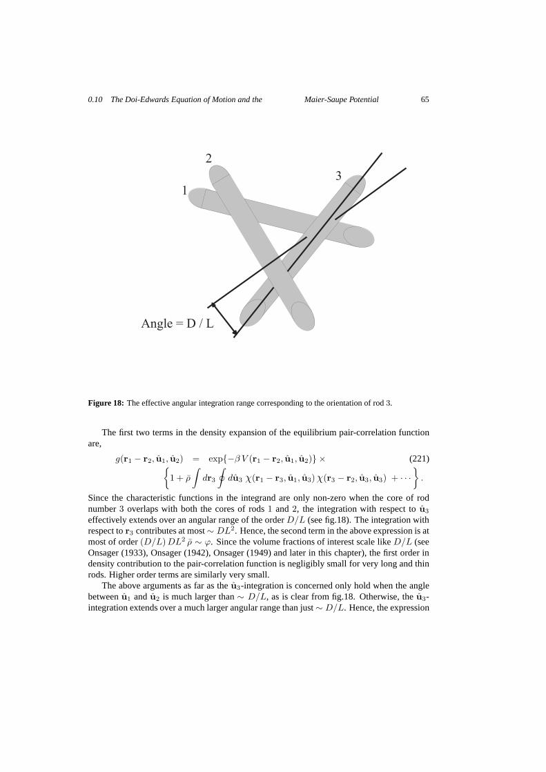
0.10 The Doi-Edwards Equation of Motion and the Maier-SaupePotential 65
1
2
3
Angle = D / L
Figure 18: The effective angular integration range corresponding to the orientation of rod3.
The first two terms in the density expansion of the equilibrium pair-correlation functionare,
g(r1 − r2, u1, u2) = exp−β V (r1 − r2, u1, u2) × (221)
1 + ρ
∫
dr3
∮
du3 χ(r1 − r3, u1, u3)χ(r3 − r2, u3, u3) + · · ·
.
Since the characteristic functions in the integrand are only non-zero when the core of rodnumber3 overlaps with both the cores of rods1 and2, the integration with respect tou3
effectively extends over an angular range of the orderD/L (see fig.18). The integration withrespect tor3 contributes at most∼ DL2. Hence, the second term in the above expression is atmost of order(D/L)DL2 ρ ∼ ϕ. Since the volume fractions of interest scale likeD/L (seeOnsager (1933), Onsager (1942), Onsager (1949) and later inthis chapter), the first order indensity contribution to the pair-correlation function is negligibly small for very long and thinrods. Higher order terms are similarly very small.
The above arguments as far as theu3-integration is concerned only hold when the anglebetweenu1 andu2 is much larger than∼ D/L, as is clear from fig.18. Otherwise, theu3-integration extends over a much larger angular range than just∼ D/L. Hence, the expression
66
(208) for the pair-correlation function is valid for high concentrations, provided that the degreeof alignment is not very high. Scaling of the angular integration range withD/L does not holdfor all configurations of the three rods. A more careful analysis shows that the second term ineq.(221) is of order(D/L) lnL/D instead ofD/L.
0.10.4 An Orientational Closure Relation
There are a number of orientational closure relations for the contraction in eq.(220) that canbe used in eq.(219) to obtain a closed equation of motion forS(t) (for an overview, see For-est and Wang (2003)). Here we will derive a simple closure relation which is shown to bereasonably accurate. It turns out that the various tumblingand wagging phenomena whererods coherently rotate under stationary shear flow (not to beconfused with the Jeffery orbitsdiscussed before) can not be accurately described by most ofthe existing closure relations.Such periodic solutions for the orientational order shouldbe analyzed on the basis of eq.(213)without using a Ginzburg-Landau expansion for| u × u
′ |.The fourth order average in eq.(220) occurs in the form of a double contraction,
A ≡ S(4) : M , (222)
whereM is equal toS. As pointed out by Hinch and Leal (1976), orientational order increasesmonotonically with increasing shear-rate, so that interpolation between the known forms forS(4) in the isotropic state and in the perfectly aligned state will probably lead to quite accurateclosures. The four point averageS(4) is known exactly for the two extreme cases of perfectalignment (along the directorn) and for the isotropic state,
< u u u u >ijkl = ninjnknl , perfect alignment,
= 115
[ δijδkl + δikδjl + δikδjl ] , isotropic, (223)
with δij the Kronecker delta (δij = 1 wheni = j, andδij = 0 wheni 6= j). Furthermore, wehave the following trivial identities,
Aij ≡∑
n,m
< ui uj un um > Mmn = Aji ,
∑
i
Aii =∑
i
∑
n,m
< ui ui un um > Mmn =∑
n,m
SnmMmn ≡ S : M . (224)
The latter identity is especially important in order to ensure that the trace ofS remains equalto 1 on time integration of the equation of motion (219). Using closures which do not satisfy(224) violate the time invariance of the trace of the order parameter. Furthermore,
A = < u u u u > : M , (225)
with,
M ≡ 12
[
M + MT]
, (226)
the symmetric part ofM, where the superscript “T ” stands for “the transpose of”. Thisequation implies that the closure relation must be a function of M.
Since order parameters tend to increase monotonically withshear rate, an accurate closurerelation can be found by constructing an interpolation formbetween the exact results (223)
0.11 Paranematic-Nematic Spinodals and the Binodal under Shear Flow 67
such that the conditions (224,225) are satisfied. Substitution of the most general form of linearcombinations of first and second order terms inS (insisting that no isotropic contributions∼ I
contribute),
A = c1S ·M + c2M · S + c3S I : M
+ c4S · S · M + c5S ·M · S + c6M · S · S + c7SS : M + c8MS : S ,
into eqs.(223-226) renders algebraic equations for the coefficientscj , leading to,
< u u u u > : M = 15
S·M + M·S− S·S·M− M·S·S + 2S·M·S + 3SS :M
. (227)
Substitution of the closure relation (227) into the equation of motion (219) finally leads to aclosed equation of motion for the orientational order parameter tensor.
The accuracy of the closure relation (227) is discussed in appendix C. Comparison of exactnumerical solutions of the Smoluchowski equation (205) fornon-interacting rods, shows thatthe closure approximation (227) withM = S and withM = E are accurate to within1% and10%, respectively. Computer simulations show that this accuracy extends to interacting rods.
0.11 Paranematic-Nematic Spinodals and the Binodalunder Shear Flow
Since shear flow tends to align rods, it will affect the location of isotropic-nematic phasetransition lines. The shear induced shift of spinodals is theoretically more easily calculated asthe shift of binodals. For the prediction of the location of binodals as a function of shear rate,equations of motion must be time-integrated up to the stationary state where two bulk phasescoexist. These equations of motion must accurately accountfor the usually sharp interfacebetween both bulk phases. Equations of this sort have been derived in Dhont and Briels (2002)and Dhont and Briels (2003) (see also the next section in thischapter as far as the stress tensoris concerned), but remain to be analyzed. On the basis of approaches that partly rely onthermodynamic arguments, similar equations of motion can be derived to predict the phasebehaviour of rods under shear flow Olmsted and Lu (1999), Olmsted (1999), Olmsted et al.(2000), Lu et al. (2000) and Fielding and Olmsted (2003). These equations of motion are inprinciple valid for small gradients in concentration and orientational order parameter, and aretherefore probably not able to accurately predict of the location of the binodal. Nevertheless,the analysis of such equations of motion reveals interesting behaviour like gradient banding,which will be discussed later in this chapter.
In the absence of flow, computer simulations where free energies are calculated can beused to obtain binodal concentrations for arbitrary aspectratios Bolhuis and Frenkel (1997).
The experimental situation is different : here it is much more difficult to measure thelocation of spinodals as compared to binodals. In the following we shall first discuss how theshear-rate dependence of spinodals can be calculated, and an experiment is discussed where aline in between the paranematic-nematic and nematic-paranematic spinodals is probed. As faras the binodal is concerned, there are no theoretical (nor simulation) results available yet. Weshall discuss an experiment where the location of the binodal is measured by means of timeresolved rheology experiments.

68
0.11.1 Spinodals
A spinodal point is defined as a point in the shear rate versus concentration diagram (theso-callednon-equilibrium phase diagram), where a stable stationary solution of the equationof motion (219) for the orientational order parameter turnsinto an unstable solution. In theabsence of shear flow, such spinodal points can also be found by means of thermodynamics.Once a solution becomes unstable, the system will start to phase separate without any timedelay. In order to describe such spinodal decomposition kinetics, one needs to consider theextension of the equation of motion (213) or (219) to inhomogeneous systems, where gradientcontributions stabilize the system against formation of very large gradients. In the absenceof shear flow, such equations of motion are analyzed by Doi et al. (1988), Shimada et al.(1988) and Winters et al. (2000). For spinodal decomposition kinetics under shear flow, theseequations of motion must be supplemented by an effective Navier-Stokes equation beyondthe initial stage of demixing. Spinodal decomposition of rod-like systems will be stronglyaffected by flow, since flow affects orientational order. Analyzing such coupled equations ofmotion as derived by Dhont and Briels (2002), Dhont and Briels (2003) is in progress. In thepresent section we shall limit the discussion to the shear induced shift of spinodals.
As far as the location of spinodals is concerned, the non-equilibrium phase diagram canmost conveniently be understood on the basis of so-calledbifurcation diagrams. A bifurcationdiagram is a plot in the orientational-order-parameter versus concentration plane, where, fora given shear rate, the order parameter for the stationary solutions of the equation of motion(219) is indicated. There are two possible stationary solutions : stable- and unstable solutions.LetS0 denote a stationary solution of eq.(219), that is, the right-hand side of eq.(219) vanishesfor S = S0. LetδS be a small perturbation. The stationary solutionS0 is referred to as a stablesolution when an initial stateS0 +δS relaxes back toS0 in time, providedδS is small enough.The stateS0 is referred to as unstable, whenδS does not relax to0, no matter how small thisperturbation is chosen. A linear stability analysis is required to decide whether a stationarysolution is either stable or unstable. Such a stability analysis for the stationary isotropic stateS0 = 1
3I in the absence of shear flow can be performed analytically. Using the closure relation
(227) in eq.(219) withγ = 0, substitution of,
S(t) = 13I + δS(t) , (228)
and linearization with respect toδS(t) readily leads to,
d
dtδS = −6Deff
r δS (229)
where,
Deffr = Dr 1 − 1
5LD
ϕ , (230)
is an effective rotational diffusion coefficient. The solution of eq.(229) reads,
δS(t) = exp
−6Deffr t
δS(t = 0) . (231)
The perturbationδS thus grows exponentially in time whenDeffr < 0, that is whenL
Dϕ > 5.
For LD
ϕ>5, the isotropic phase becomes unstable, and the new stable state is the nematic statewith a relatively large value forλ. On subsequently lowering the concentration, the nematicstate becomes unstable atL
Dϕ<40/9 = 4.44 · · · , and the system returns to the isotropic state.
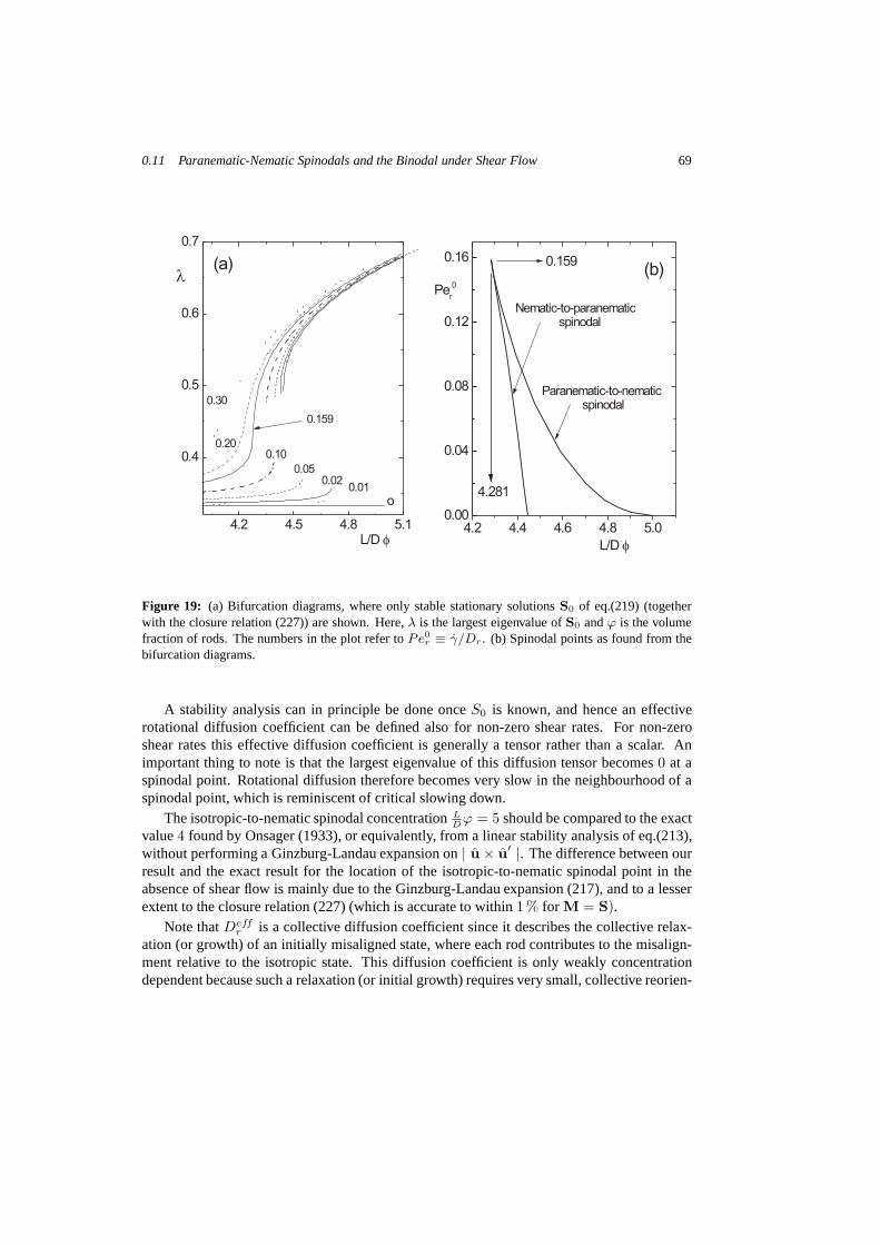
0.11 Paranematic-Nematic Spinodals and the Binodal under Shear Flow 69
4.2 4.5 4.8 5.1
0.4
0.5
0.6
0.7
0.159
(a)
0.20
0.30
0.10
0.050.02
0.01
o
l
L/D f4.2 4.4 4.6 4.8 5.0
0.00
0.04
0.08
0.12
0.16
4.281
0.159
Paranematic-to-nematicspinodal
Nematic-to-paranematicspinodal
(b)Pe
r
0
L/D f
Figure 19: (a) Bifurcation diagrams, where only stable stationary solutionsS0 of eq.(219) (togetherwith the closure relation (227)) are shown. Here,λ is the largest eigenvalue ofS0 andϕ is the volumefraction of rods. The numbers in the plot refer toPe0
r ≡ γ/Dr. (b) Spinodal points as found from thebifurcation diagrams.
A stability analysis can in principle be done onceS0 is known, and hence an effectiverotational diffusion coefficient can be defined also for non-zero shear rates. For non-zeroshear rates this effective diffusion coefficient is generally a tensor rather than a scalar. Animportant thing to note is that the largest eigenvalue of this diffusion tensor becomes0 at aspinodal point. Rotational diffusion therefore becomes very slow in the neighbourhood of aspinodal point, which is reminiscent of critical slowing down.
The isotropic-to-nematic spinodal concentrationLD
ϕ = 5 should be compared to the exactvalue4 found by Onsager (1933), or equivalently, from a linear stability analysis of eq.(213),without performing a Ginzburg-Landau expansion on| u × u
′ |. The difference between ourresult and the exact result for the location of the isotropic-to-nematic spinodal point in theabsence of shear flow is mainly due to the Ginzburg-Landau expansion (217), and to a lesserextent to the closure relation (227) (which is accurate to within 1 % for M = S).
Note thatDeffr is a collective diffusion coefficient since it describes thecollective relax-
ation (or growth) of an initially misaligned state, where each rod contributes to the misalign-ment relative to the isotropic state. This diffusion coefficient is only weakly concentrationdependent because such a relaxation (or initial growth) requires very small, collective reorien-
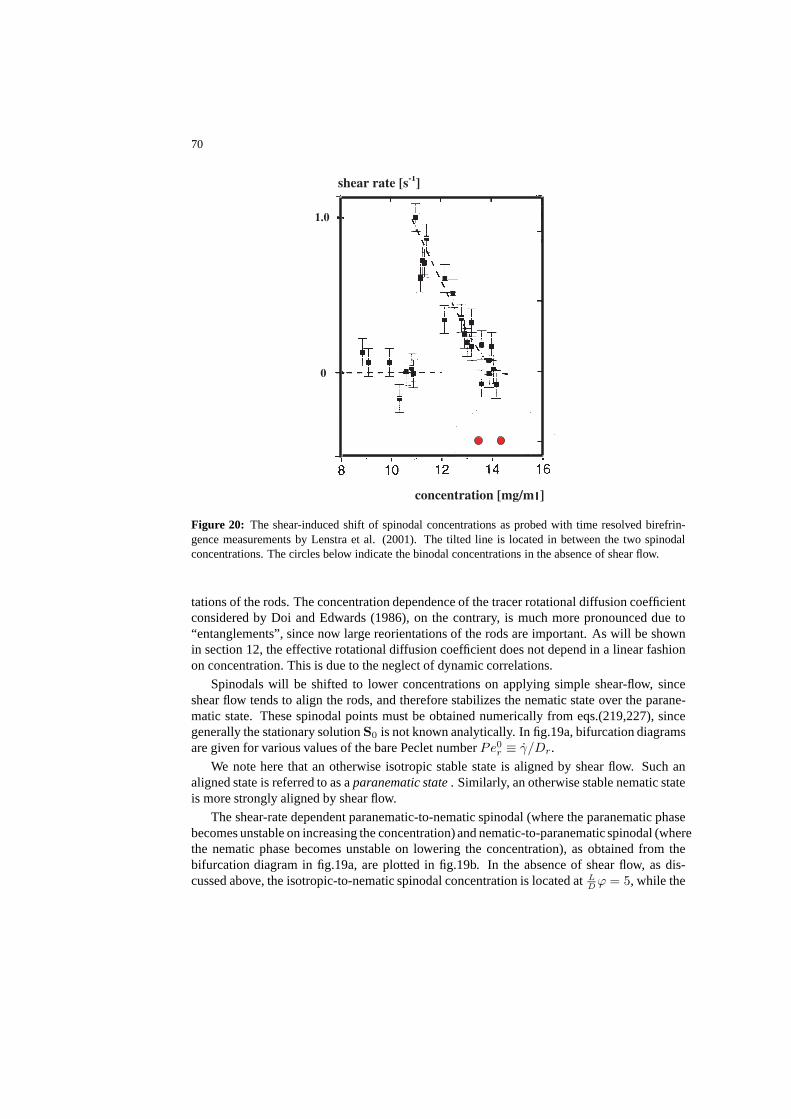
70
shear rate [s-1
]
concentration [mg/m ]
1.0
0
l
Figure 20: The shear-induced shift of spinodal concentrations as probed with time resolved birefrin-gence measurements by Lenstra et al. (2001). The tilted lineis located in between the two spinodalconcentrations. The circles below indicate the binodal concentrations in the absence of shear flow.
tations of the rods. The concentration dependence of the tracer rotational diffusion coefficientconsidered by Doi and Edwards (1986), on the contrary, is much more pronounced due to“entanglements”, since now large reorientations of the rods are important. As will be shownin section 12, the effective rotational diffusion coefficient does not depend in a linear fashionon concentration. This is due to the neglect of dynamic correlations.
Spinodals will be shifted to lower concentrations on applying simple shear-flow, sinceshear flow tends to align the rods, and therefore stabilizes the nematic state over the parane-matic state. These spinodal points must be obtained numerically from eqs.(219,227), sincegenerally the stationary solutionS0 is not known analytically. In fig.19a, bifurcation diagramsare given for various values of the bare Peclet numberPe0
r ≡ γ/Dr.
We note here that an otherwise isotropic stable state is aligned by shear flow. Such analigned state is referred to as aparanematic state. Similarly, an otherwise stable nematic stateis more strongly aligned by shear flow.
The shear-rate dependent paranematic-to-nematic spinodal (where the paranematic phasebecomes unstable on increasing the concentration) and nematic-to-paranematic spinodal (wherethe nematic phase becomes unstable on lowering the concentration), as obtained from thebifurcation diagram in fig.19a, are plotted in fig.19b. In theabsence of shear flow, as dis-cussed above, the isotropic-to-nematic spinodal concentration is located atL
Dϕ = 5, while the
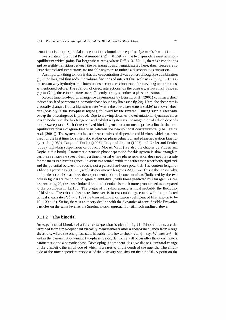
0.11 Paranematic-Nematic Spinodals and the Binodal under Shear Flow 71
nematic-to-isotropic spinodal concentration is found to be equal toLD
ϕ = 40/9 = 4.44 · · · .For a critical rotational Peclet numberPe0
r = 0.159 · · · , the two spinodals meet in a non-equilibrium critical point. For larger shear-rates, wherePe0
r > 0.159 · · · , there is a continuousand reversible transition between the paranematic and nematic state : here, shear forces are solarge that rod-rod interactions are not able anymore to induce a discontinuous transition.
An important thing to note is that the concentration always enters through the combinationLD
ϕ. For long and thin rods, the volume fractions of interest thus scale as∼ DL≪ 1. This is
the reason why hydrodynamic interactions become less important for very long and thin rods,as mentioned before. The strength of direct interactions, on the contrary, is not small, since atLD
ϕ = O(1), these interactions are sufficiently strong to induce a phase transition.Recent time resolved birefringence experiments by Lenstraet al. (2001) confirm a shear
induced shift of paranematic-nematic phase boundary lines(see fig.20). Here, the shear rate isgradually changed from a high shear rate (where the one-phase state is stable) to a lower shearrate (possibly in the two-phase region), followed by the reverse. During such a shear-ratesweep the birefringence is probed. Due to slowing down of theorientational dynamics closeto a spinodal line, the birefringence will exhibit a hysteresis, the magnitude of which dependson the sweep rate. Such time resolved birefringence measurements probe a line in the non-equilibrium phase diagram that is in between the two spinodal concentrations (see Lenstraet al. (2001)). The system that is used here consists of dispersions of fd virus, which has beenused for the first time for systematic studies on phase behaviour and phase separation kineticsby et al. (1989), Tang and Fraden (1993), Tang and Fraden (1995) and Grelet and Fraden(2003), including suspensions of Tobacco Mosaic Virus (seealso the chapter by Fraden andDogic in this book). Paranematic-nematic phase separationfor this system is slow enough toperform a shear-rate sweep during a time interval where phase separation does not play a rolefor the measured birefringence. Fd-virus is a semi-flexiblerod rather then a perfectly rigid rod,and the potential between the rods is not a perfect hard-corepotential. The contour length ofa fd-virus particle is880 nm, while its persistence length is2200 nm. This is the reason why,in the absence of shear flow, the experimental binodal concentrations (indicated by the twodots in fig.20) are found not to agree quantitatively with those predicted by Onsager. As canbe seen in fig.20, the shear-induced shift of spinodals is much more pronounced as comparedto the prediction in fig.19b. The origin of this discrepancy is most probably the flexibilityof fd virus. The critical shear rate, however, is in reasonable agreement with the predictedcritical shear ratePe0
r ≈ 0.159 (the bare rotational diffusion coefficient of fd is known to be10 − 20 s−1). So far, there is no theory dealing with the dynamics of semi-flexible Brownianparticles on the same level as the Smoluchowski approach forstiff rods outlined above.
0.11.2 The binodal
An experimental binodal of a fd-virus suspension is given infig.21. Binodal points are de-termined from time-dependent viscosity measurements after a shear-rate quench from a highshear rate, where the one-phase state is stable, to a lower shear rate,γ− say. Wheneverγ− iswithin the paranematic-nematic two-phase region, demixing will occur after the quench into aparanematic and a nematic phase. Developing inhomogeneities give rise to a temporal changeof the viscosity, the amplitude of which increases with the depth of the quench. The ampli-tude of the time dependent response of the viscosity vanishes on the binodal. A point on the
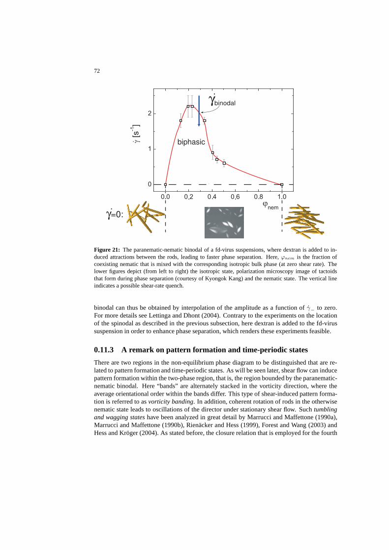
72
.
. .....
biphasic
γbinodal
.
γ=0:.
Figure 21: The paranematic-nematic binodal of a fd-virus suspensions, where dextran is added to in-duced attractions between the rods, leading to faster phaseseparation. Here,ϕnem is the fraction ofcoexisting nematic that is mixed with the corresponding isotropic bulk phase (at zero shear rate). Thelower figures depict (from left to right) the isotropic state, polarization microscopy image of tactoidsthat form during phase separation (courtesy of Kyongok Kang) and the nematic state. The vertical lineindicates a possible shear-rate quench.
binodal can thus be obtained by interpolation of the amplitude as a function ofγ− to zero.For more details see Lettinga and Dhont (2004). Contrary to the experiments on the locationof the spinodal as described in the previous subsection, here dextran is added to the fd-virussuspension in order to enhance phase separation, which renders these experiments feasible.
0.11.3 A remark on pattern formation and time-periodic states
There are two regions in the non-equilibrium phase diagram to be distinguished that are re-lated to pattern formation and time-periodic states. As will be seen later, shear flow can inducepattern formation within the two-phase region, that is, theregion bounded by the paranematic-nematic binodal. Here “bands” are alternately stacked in the vorticity direction, where theaverage orientational order within the bands differ. This type of shear-induced pattern forma-tion is referred to asvorticity banding. In addition, coherent rotation of rods in the otherwisenematic state leads to oscillations of the director under stationary shear flow. Suchtumblingand wagging stateshave been analyzed in great detail by Marrucci and Maffettone (1990a),Marrucci and Maffettone (1990b), Rienacker and Hess (1999), Forest and Wang (2003) andHess and Kroger (2004). As stated before, the closure relation that is employed for the fourth
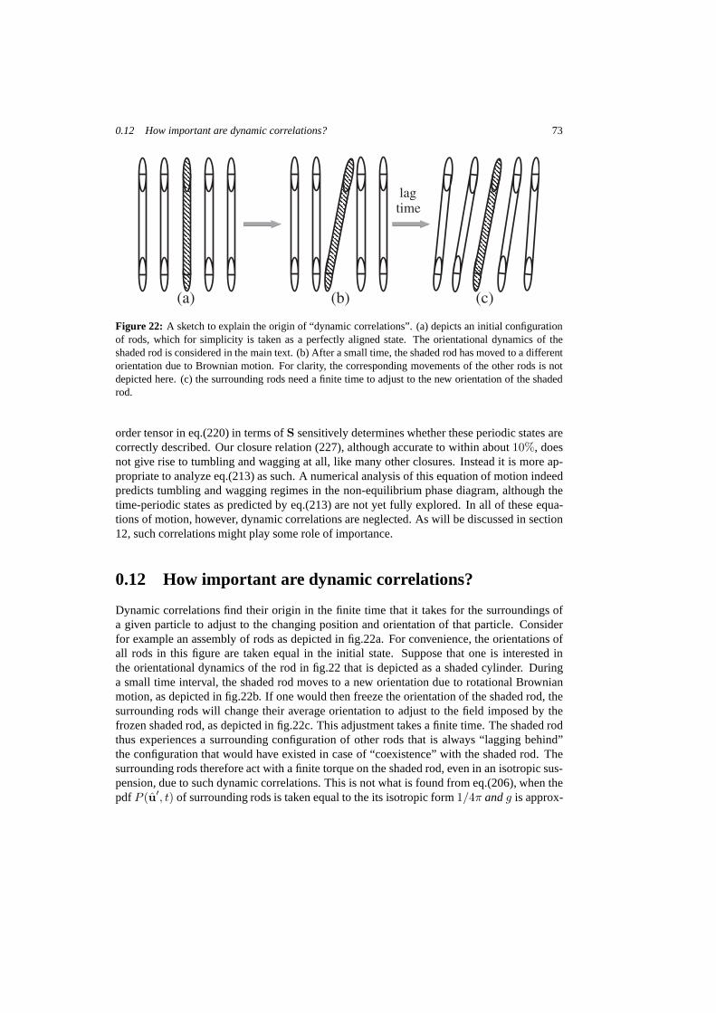
0.12 How important are dynamic correlations? 73
lagtime
(a) (b) (c)
Figure 22: A sketch to explain the origin of “dynamic correlations”. (a) depicts an initial configurationof rods, which for simplicity is taken as a perfectly alignedstate. The orientational dynamics of theshaded rod is considered in the main text. (b) After a small time, the shaded rod has moved to a differentorientation due to Brownian motion. For clarity, the corresponding movements of the other rods is notdepicted here. (c) the surrounding rods need a finite time to adjust to the new orientation of the shadedrod.
order tensor in eq.(220) in terms ofS sensitively determines whether these periodic states arecorrectly described. Our closure relation (227), althoughaccurate to within about10%, doesnot give rise to tumbling and wagging at all, like many other closures. Instead it is more ap-propriate to analyze eq.(213) as such. A numerical analysisof this equation of motion indeedpredicts tumbling and wagging regimes in the non-equilibrium phase diagram, although thetime-periodic states as predicted by eq.(213) are not yet fully explored. In all of these equa-tions of motion, however, dynamic correlations are neglected. As will be discussed in section12, such correlations might play some role of importance.
0.12 How important are dynamic correlations?
Dynamic correlations find their origin in the finite time thatit takes for the surroundings ofa given particle to adjust to the changing position and orientation of that particle. Considerfor example an assembly of rods as depicted in fig.22a. For convenience, the orientations ofall rods in this figure are taken equal in the initial state. Suppose that one is interested inthe orientational dynamics of the rod in fig.22 that is depicted as a shaded cylinder. Duringa small time interval, the shaded rod moves to a new orientation due to rotational Brownianmotion, as depicted in fig.22b. If one would then freeze the orientation of the shaded rod, thesurrounding rods will change their average orientation to adjust to the field imposed by thefrozen shaded rod, as depicted in fig.22c. This adjustment takes a finite time. The shaded rodthus experiences a surrounding configuration of other rods that is always “lagging behind”the configuration that would have existed in case of “coexistence” with the shaded rod. Thesurrounding rods therefore act with a finite torque on the shaded rod, even in an isotropic sus-pension, due to such dynamic correlations. This is not what is found from eq.(206), when thepdf P (u′, t) of surrounding rods is taken equal to the its isotropic form1/4π andg is approx-
74
imated by the Boltzmann exponential (208). In order to describe self rotational diffusionof arod on the basis of eq.(206), dynamic correlations are essential.
The neglect of dynamic correlations in the derivation of theDoi-Edwards equation (219)becomes more clear on calculating the correlation function< u(t) · u(0) > for an isotropicdispersion. Thus, consider a rod (the dashed rod in fig.22) with a specified orientationu(0) attime t = 0. Noting that,
d
dt< u(t) · u(0) > = u(0) ·
∮
du u∂P (u, t)
∂t
multiplying both sides of the Smoluchowski equation (206) with u · u(0) and integrating withrespect tou readily leads to,
d
dt< u(t) · u(0) > = −2 Deff
s (t) < u(t) · u(0) > , (232)
where the effective self-rotational diffusion coefficientis equal to,
Deffs (t) ≡ Dr
1 − 12β
< T(u(t)) · (u(t) × u(0)) >
< u(t) · u(0) >
, (233)
where the torqueT(u(t)) is given by eq.(206) with an obvious change of notation. The pdfP (u′, t) in the expression (206) for the torque is that of the other rods (the non-dashed rods infig.22). When the pdfP (u′, t) of the other rods is taken equal to1/4π and approximating thepair-correlation function with the Boltzmann exponential(208), one finds thatT(u(t)) = 0.Hence,Deff
s (t) = Dr which is obviously wrong, since rotational motion of the dashed rodis certainly hindered by the presence of other rods. A non-zero torque results from dynamiccorrelations :P (u′, t) of rods in the neighbourhood of the dashed rod differs from1/4π dueto the presence of the moving dashed rod, and the pair-correlation function is not equal to theequilibrium Boltzmann exponential for the same reason.
The linear concentration dependence of the effective diffusion coefficient (230), which isa collective diffusion coefficient, is entirely due to the neglect of dynamic correlations. MDcomputer simulations, where the tail of the orientational correlation function is fitted to obtainthe effective diffusion coefficient, show a strong non-linear concentration dependence Taoet al. (2004), as is shown in fig.23. This indicates that dynamic correlations are of importance.As yet, no attempt has been made to incorporate dynamic correlations in the analysis of theSmoluchowski equation (206). As will be seen later, computer simulations do predict a linearconcentration dependence of the shear viscosity. It thus seems that dynamic correlations. areof minor importance for the viscoelastic response of suspensions of rods, contrary to diffusivebehaviour.
0.13 The Stress Tensor for Rod Suspensions
In addition to the orientational order of rods in shear flow, the viscous behaviour of thesesystems is of interest. In this section we shall derive a microscopic expression for the stresstensor and express it in terms of the orientational order parameter tensor (see also Dhontand Briels (2002) and Dhont and Briels (2003)). Viscoelastic response functions can then becalculated once the equation of motion (219) forS(t) is solved.

0.13 The Stress Tensor for Rod Suspensions 75
0.0 0.5 1.0 1.50.0
0.5
1.0
Dr
eff/ D
r
(L/D) f
Figure 23: The effective diffusion coefficient as defined in the previous section from the theory eq.(230)where dynamic correlations are neglected and from simulations by Tao et al. (2004) (the solid linethrough simulation data points are a guide to the eye.)
0.13.1 The basic idea
Let U(r, t) andρm(r, t) denote the suspension velocity and mass density, respectively. Thevelocity satisfies the Navier-Stokes equation (13), were the divergence of the stress tensor isaveraged over the phase space coordinatesΓ of the colloidal rods,
ρm(r, t)
[
∂U(r, t)
∂t+ U(r, t) · ∇U(r, t)
]
= < ∇ · σ(r | Γ(t)) > . (234)
Here,σ is the stress tensor of the solvent in which the rods are embedded, or of the corematerial of the rods, depending on whetherr is within the solvent or inside the core of a rod.Clearly,σ depends on the phase space coordinatesΓ of all the rods.
The fundamental quantity in hydrodynamics is the momentum densityρv, with ρ andv
the microscopic density and velocity, respectively. Therefore, the appropriate definition of themacroscopic velocityU is,
ρm(r, t)U = < ρv > . (235)
It can be shown (see Dhont and Briels (2002)) that if the mass density between the fluid andthe core material of which the rods consist and/or the volumefraction of colloidal material isvery small, the definition in eq.(235) reduces simply to,
U(r, t) = < v(r |Γ(t)) > , (236)
76
whereu is equal to the fluid velocity or the velocity of a piece of colloidal material, dependingon whetherr is within the solvent or inside the core of a colloidal rod.
Let P (Γ, t) denote the probability density function ofΓ, which is the solution of theSmoluchowski equation (173). By definition we then have,
U(r, t) =
∫
dΓP (Γ, t)v(r |Γ) . (237)
In the derivation of the general expression for the divergence of the stress tensor, we shallencounter the ensemble average,
< ∇2v(r) > =
∫
dΓP (Γ, t)∇2v(r |Γ) .
Since the Laplace operator can be taken in front of the phase-space integral, and the suspensionflow velocity is given by eq.(236), it trivially follows that,
< ∇2v(r) > = ∇2U(r, t) . (238)
This result will be of importance later in this section.In order to obtain an explicit Navier-Stokes equation, the ensemble average of the body
force∇ · σ(r | Γ) should be expressed in terms of suspension properties. To this end, con-sider a rectangular volume elementδV located atr, with linear dimensionsδx, δy andδz inthe x−, y− andz−direction, respectively. In the formal limit that the size of the volumeelement vanishes, the ensemble averaged total force per unit volume of the surrounding ma-terial on the volume element is nothing but the divergence ofthe stress tensor that should beused in the Navier-Stokes equation (234). This force consists of three parts : forces that arisefrom interactions between colloidal particles outside on those within the rectangular volumeelement, from interactions between solvent molecules and colloidal particles, and from inter-actions between solvent molecules on either side of the boundary of the volume element. Thecorresponding stress tensors will be referred to as the “particle-particle stress tensor”Σpp, the“particle-solvent stress tensor”Σps, and the “solvent-solvent stress tensor”Σss, respectively.The divergence of the suspension stress tensorΣ is the sum of these three body forces,
∇ · Σ ≡ < ∇ · σ(r | Γ(t)) > = ∇ ·Σpp + ∇ · Σps + ∇ · Σss . (239)
These three contributions will be calculated explicitly inthe next subsections. First of all, ageneral expression for the ensemble averaged body force∇ · Σ will be derived, after whichthis expression will be expressed in terms of a probability density density function. Finally,this expression will be simplified by means of the same Ginsburg-Landau expansion used toderive the Doi-Edwards equation (219), which leads to an expression for the stress tensorinvolving the concentration and the orientational order parameter tensorS.
The particle-particle stress tensorΣpp
The force that colloidal particles outside the volume element exert on those within the volumeelement is equal to,
⋆∑
j
Fj ,
0.13 The Stress Tensor for Rod Suspensions 77
whereFj is the force that all colloidal particles exert on colloidalparticlej, and the⋆ on thesummation is used to indicate that the summation ranges onlyover those colloidal particlesthat are inside the volume element, that is, for whichrj ∈ δV . Note that mutual interactionsbetween colloidal particles within the volume element can not give rise to a net force onthat volume element. The force per unit volume, for formallyvanishing size of the volumeelement, is thus equal to,
∇ ·Σpp = limδx,δy,δz→0
1
δx δy δz
N∑
j=1
< χr(rj)Fj > , (240)
whereN is the total number of colloidal particles in the system under consideration,rj is theposition coordinate of a colloidal particle andχ
ris the characteristic function of the rectan-
gular volume element that was introduced in the previous section. The characteristic functionis defined as,
χr(R) = 1 when R ∈ δV ,
= 0 otherwise. (241)
The subscript “r ” on the characteristic function is used to indicate that thevolume elementδV is located at positionr. The characteristic function effectively limits the summation tocolloidal particles that are insideδV , that is, for whichrj ∈ δV . Furthermore, as discussedbefore, the total forceFj on thejth colloidal particle due to interactions with all other colloidalparticles is equal to,
Fj = −∇jΦ − kBT∇j lnP , (242)
whereΨ is the total potential energy of the assembly ofN rods in the suspension, andP is theprobability density function of the phase space coordinates of all the colloidal rods :−∇jΦis the force due to potential interactions, and−kBT∇j lnP is the Brownian force, where∇j is the gradient operator with respect torj . Since (withδ(r − rj) the 3-dimensional deltadistribution),
limδx,δy,δz→0
χr(rj)/δx δy δz = δ(r − rj) , (243)
as is easily verified by integration of both sides with respect to rj , this immediately leads to,
∇ ·Σpp =
N∑
j=1
< δ(r − rj) Fj > . (244)
Together with eq.(242) for the forces, this is the microscopic expression for the contributionto the divergence of the stress tensor which is due to inter-colloidal particle forces.
The particle-solvent stress tensorΣps
The particle-solvent stress arises from forces on the volume element due to interactions be-tween colloidal particles and solvent molecules. These forces are mediated to the volumeelement by colloidal particles that intersect with the surface enclosing the rectangular volumeelement. Consider first the force that is mediated to the solvent within the volume element by

78
zd
x
y
z
( )in
jV
( )out
jV
yd
xd
r
Figure 24: The rectangular volume elementδV at positionr intersects with the core of colloidal rodjwith its position coordinaterj outside the volume element.∂V (out) is that part of the surface area∂Vj
of the rod that is outside the volume element, and∂V(in)j is the part inside.
a colloidal particle with its position coordinate outside the volume element (see fig.24). Theinstantaneous force that the colloidal particle exerts on the solvent inside the volume elementis equal to,
−∫
∂V(in)
j(rj ,uj)
dS′ · σ(r′) .
Here, the surface area∂V(in)j is that part of the surface area of the colloidal particle that is
inside the volume element (see fig.24). This range of integration depends both on the positionrj of colloidal particlej and its orientationuj . Furthermore,dS′ is the normal surface elementon the surface area of the colloidal particle, andσ is the stress tensor of the solvent. The minussign in eq.(245) arises from the fact thatdS′ ·σ(r′) is equal todS′ fh(r′), with fh(r′) the forceper unit area that the fluid exerts on the surface elementdS′, which is minus the force that thissurface element exerts on the fluid. In terms of this hydrodynamic force, eq.(245) is moreconveniently written as,
−∫
∂V(in)
j(rj ,uj)
dS′ fh(r′) .
0.13 The Stress Tensor for Rod Suspensions 79
The ensemble averaged forceFout of all colloidal particles outside the volume element on thesolvent inside the element, is thus equal to,
Fout = − <
N∑
j=1
[1 − χr(rj)]
∮
∂Vj(rj ,uj)
dS′ fh(r′)χr(r′) > , (245)
where, as before,χr
is the characteristic function of the volume element. The characteristicfunction1−χ
r(rj) for the volume outside the volume element assures that in thesummation
over all colloidal particles, only those are counted which are outside the volume element. Fur-thermore, the characteristic functionχ
r(r′) assures that only pointsr′ on the surface of the
colloidal particle inside the volume element are taken intoaccount. Including the character-istic function in the integrand in eq.(245) allows for the extension of the integration range tothe entire surface area∂Vj(rj , uj) of thejth colloidal particle.
Similarly, in case a colloidal particle is located inside the volume element, that is, whenrj ∈ δV , the instantaneous force that the colloidal particle exerts on the solvent outside thevolume element is equal to,
−∫
∂V(out)
j(rj ,uj)
dS′ fh(r′) ,
with ∂V(out)j the part of the surface area of the colloidal particle located outside the volume
element (see fig.24. This is minus the force that is exerted onthe colloidal particle by thesolvent outside the volume element. Hence, similarly as before, the ensemble averaged forceFin on the volume element due to interactions between solvent molecules outside and col-loidal particles inside the volume element is found to be equal to,
Fin = <N
∑
j=1
χr(rj)
∮
∂Vj(rj ,uj)
dS′ fh(r′) [1 − χr(r′)] > , (246)
where it is used again that1 −χr(r′) is the characteristic function for the volume outside the
volume element. From the representation (243) of the delta distribution it is thus found that,
∇ ·Σps = limδx,δy,δz→0
[
Fout + Fin]
/δx δy δz (247)
= <N
∑
j=1
δ(r − rj)Fhj > − <
N∑
j=1
∮
∂Vj(rj ,uj)
dS′ δ(r − r′) fh(r′) > ,
where,
Fhj =
∮
∂Vj(rj ,uj)
dS′ fh(r′) , (248)
is the total force that the solvent exerts on thejth colloidal particle.
The solvent-solvent stress tensorΣss
The force per unit volume that the solvent outside the volumeelementδV exerts on the solventinside, for formally vanishing size of the volume element, is equal to,
∇ ·Σss = limδx,δy,δz→0
1
δx δy δz<
∫
As
dS′ · σ(r′) > , (249)
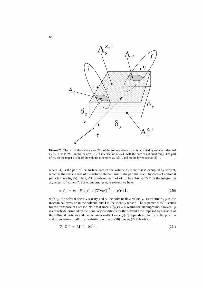
80
+z,sA
j'A j'
jr
j
zd
+z,sA
·
r
·
jA·
'jr
x
y
z
x
y
zyd
xd
Figure 25: The part of the surface area∂δV of the volume element that is occupied by solvent is denotedasAs. This is∂δV minus the areasAj of intersection of∂δV with the core of colloidal rodj. The partof As on the upperz-side of the volume is denoted asAz,+
s , and on the lower side asAz,−s .
whereAs is the part of the surface area of the volume element that is occupied by solvent,which is the surface area of the volume element minus the partthat is cut by cores of colloidalparticles (see fig.25). Here,dS′ points outward ofδV . The subscript “s ” on the integrationAs refers to “solvent”. For an incompressible solvent we have,
σ(r′) = η0
[
∇′v(r′) + (∇′v(r′))T
]
− p(r′) I , (250)
with η0 the solvent shear viscosity andv the solvent flow velocity. Furthermore,p is themechanical pressure in the solvent, andI is the identity tensor. The superscript “T ” standsfor the transpose of a tensor. Note that since∇2p(r) = 0 within the incompressible solvent,pis entirely determined by the boundary conditions for the solvent flow imposed by surfaces ofthe colloidal particles and the container walls. Hence,p(r′) depends implicitly on the positionand orientations of all rods. Substitution of eq.(250) intoeq.(249) leads to,
∇ · Σss = M(1) + M(2) , (251)

0.13 The Stress Tensor for Rod Suspensions 81
where,
M(1) ≡ limδx,δy,δz→0
η0
δx δy δz<
∫
As
dS′ ·[
∇′v(r′) + (∇′v(r′))T
]
> , (252)
and,
M(2) ≡ − limδx,δy,δz→0
1
δx δy δz<
∫
As
dS′ p(r′) > , (253)
Consider first the contributionM(1). We can rewrite the integral as,
<
∫
As
dS′ ·[
∇′v(r′)+(∇′v(r′))T]
> = <
∮
∂δV
−N
∑
j=1
∫
Aj
dS′ ·[
∇′v(r′)+(∇′v(r′))T]
>,
(254)
whereAj is the area of intersection of the surface area∂δV of the volume element and thecore of colloidal particlej (see fig.25). For a rigid colloidal particle, the velocity inside thecore is given by,
v(r′) = vj + Ωj × (r′ − rj) , r′ ∈ core of particlej , (255)
wherevj is the translational velocity andΩj the rotational velocity of colloidal particlej.Hence (withǫ the Levi-Cevita tensor, andΩj,p thepth component ofΩj),
∇′m vn = ∇m [Ωj × (r′ − rj) ]n = ∇′
m ǫnpq Ωj,p r′q = ǫnpm Ωj,p ,
where summation over repeated indices is assumed. From the anti-symmetry of the Levi-Cevita tensor, it is thus found that,
∫
Aj
dS′ ·[
∇′v(r′) + (∇′v(r′))T
]
= 0 . (256)
Using Gauss’s integral theorem, we thus find from eqs.(254,256), for incompressible solvents,
<
∫
As
dS′ ·[
∇′v(r′)+(∇′v(r′))T
]
> = <
∫
δV
dr′ ∇′ 2v(r′) > ,
Hence, eq.(252) reduces to,
M(1) = limδx,δy,δz→0
η0
δx δy δz<
∫
δV
dr′ ∇′ 2v(r′)> = η0 < ∇2v(r) > .
From eq.(238), it is thus finally found that,
M(1) = η0 ∇2U(r, t) . (257)
The contributionM(2) can be expressed in terms of suspension properties as follows. LetAz,+
s denote the top-side ofAs, and similarlyAz,−s the lower-side, as indicated in fig.25.
Furthermore, letez denote the unit vector along the positivez-axis. Since the unit normal onAz,+
s is ez while the unit normal onAz,−s is −ez, the contributionM(2)
z from the top- andlower-side ofAs to M(2) is equal to,
M(2)z = −ez lim
δx,δy,δz→0
1
δx δy δz<
[∫
Az,+s
−∫
Az,−s
]
dS′ p(r′) > .
82
For small sizes of the volume element, the scalar,
P ss(r + 12δz ez, t) ≡ 1
δx δy<
∫
Az,+s
dS′ p(r′) > , (258)
defines the contribution to the suspension pressure due solvent-solvent interactions at the po-sition of the top-side of the volume element. A similar expression can be written down forP ss at the lower-side. It thus follows that,
M(2)z = −ez lim
δz→0
1
δz[P ss(r + 1
2δz ez, t) − P ss(r − 1
2δz ez, t)] = −ez
∂P ss(r, t)
∂z.
In the same way the contribution toM(2) from the left- and right-sides, and front- and back-sides of the volume element are obtained. Adding these contributions leads to,
M(2) = −∇P ss(r, t) . (259)
We thus find from eqs.(251,257,259) the following expression for the divergence of thestress tensor that arises from solvent-solvent interactions,
∇ · Σss = η0 ∇2U(r, t) −∇P ss(r, t) . (260)
Note thatP ss is not just determined by boundary conditions when the suspension is inhomo-geneous.
0.13.2 The total stress tensor
On the Smoluchowski time scale, as discussed before, the interaction forceFj in eq.(242)balances with the hydrodynamic force in eq.(248), that is,
Fj + Fhj = 0 . (261)
The first term in eq.(247) for the particle-solvent stress thus cancels against the particle-particle stress in eq.(244). Adding eqs.(244,247,260) therefore leads to the following ex-pression for the divergence of the total stress tensor,
∇ · Σ = η0 ∇2U(r, t) −∇P ss(r, t) −N
∑
j=1
<
∮
∂Vj(rj ,uj)
dS′ δ(r − r′) fh(r′) > . (262)
This seemingly simple expression is valid for homogeneous suspensions as well as systemswith large gradients in shear rate, concentration and orientational order parameter. Suspensionproperties should not vary significantly over distances equal to the thickness of the rods, butmay vary significantly over distances equal to the length of the rods.
0.13.3 The stress tensor for homogeneous suspensions
Sincer′ ∈ ∂Vj in the integrand in eq.(262), the magnitude ofr′ − rj is never larger thanthe linear dimension of the rigid colloidal particles. Hence, for not too large gradients ofsuspension properties, the delta distributionδ(r− r′) can be Taylor expanded aroundr′ = rj ,
δ(r − r′) = δ(r − rj) +
∞∑
n=1
1
n!(rj − r′)n ⊙∇nδ(r − rj) ,

0.13 The Stress Tensor for Rod Suspensions 83
where(rj − r′)n and∇n are polyadic products, and⊙ is then-fold contraction of these twoproducts. Substitution of this expansion into eq.(262) gives,
∇ · Σ = η0 ∇2U(r, t) −∇P ss(r, t) −N
∑
j=1
< δ(r − rj) Fhj > (263)
−∞∑
n=1
1
n!∇n
N∑
j=1
< δ(r − rj) ⊙∮
∂Vj(rj ,uj)
dS′ (rj − r′)n fh(r′) > .
Consider a flow in thex-direction with its gradient in they-direction (see fig.1a). Since allsuspension properties, including the suspension flow velocity, do not vary onxz-planes, thestress tensor is a function ofy only. Hence,
∇ ·Σ(r) = e2 ·dΣ(y)
dy.
where e2 is the unit vector in they-direction. Since in a homogeneous system the force<δ(r − rj)F
hj > on rodj atr is independent ofr, it follows that the contribution∆Σ to the
stress tensor corresponding to the last term in the first linein eq.(263) is equal to,
e2 · ∆Σ(y) = −y
N∑
j=1
< δ(r − rj)Fhj > = − e2 ·
N∑
j=1
< δ(r − rj) rj Fhj > .
Here, the integration constant is set equal to0, since it does not contribute to the force on agiven volume element, and is therefore irrelevant. Hence,
∆Σ = −N
∑
j=1
< δ(r − rj) rj Fhj > . (264)
In the last term in eq.(263), only the leading order gradientcontribution is non-zero for homo-geneous suspensions, so that,
∞∑
n=1
1
n!∇n
N∑
j=1
< δ(r − rj) ⊙∮
∂Vj(rj ,uj)
dS′ (rj − r′)n fh(r′) > =
−∇ ·N
∑
j=1
< δ(r − rj)
∮
∂Vj(rj ,uj)
dS′ (r′ − rj) fh(r′) > . (265)
From eqs.(263,264,265), the stress tensor is found to be equal to,
Σ = η0
[
∇U + (∇U)T
]
− P ss I−N
∑
j=1
< δ(r − rj) rj Fhj >
+
N∑
j=1
< δ(r − rj)
∮
∂Vj(rj ,uj)
dS′ (r′ − rj) fh(r′) > . (266)
On volume averaging, one recovers the expression for the stress tensor as derived by Batchelor(1970) and later by Strating (1995) in different ways. Note that a divergence-less contributionto the stress tensor is of no significance, since the suspension flow velocity is determinedsolely by the body force that is equal to the divergence of thestress tensor.

84
0.13.4 Explicit evaluation of the stress tensorfor very Long and thin rods
Within the bead model for the rods (see fig.3), the surface integral that appears in eq.(262) forthe stress tensor can be written as a sum over beads as (with∂Vα the surface area of beadα),
∮
∂Vj(rj ,uj)
dS′ δ(r−r′) fh(r′) =∑
α
δ(r−rj−α Duj)Fhj,α ,
whereFhj,α is the force that the fluid exerts on theα’th bead of rodj. Hence,
∇ · Σ = η0∇2U(r, t) −∇P ss(r, t) −N
∑
j=1
∑
α
< δ(r − rj − α D uj)Fhj,α > . (267)
In order to evaluate the summation over beads, an explicit expression forFhj,α must be found.
Consider the flow velocityu0,α of the fluid that would have existed in the absence of beadα.This velocity is equal to, according to eq.(18),
u0,α = U⋆α −
∑
β 6=α
∫
∂Vβ
dS′ T(rα − r′) · fh,⋆β (r′) , (268)
where the⋆ is used to indicate the absence of beadα. Here,U⋆ is the fluid flow velocity at theposition of beadα that is due to the presence of the remaining rods and the externally imposedflow field, in the absence of beadα. The forcefh,⋆
β (r′) is the force per unit area that the fluidexerts on the surface element atr′ on the surface∂Vβ of beadβ, again in the absence of beadα. For very long and thin rods, the majority of beadsβ experience a flow and force that isonly a little different from those in the absence of beadα. We shall therefore setfh,⋆
β equalto the actual forcefh
β in the presence of beadα. Within the bead model for the rod, eq.(268)then reads,
u0,α = U⋆α −
∑
β 6=α
T(rα − rβ) · Fhβ , (269)
where, as before,Fhβ is the total force that the fluid exerts on beadβ. When gradients in
the fluid flow velocityU⋆α, stemming from other rods and an externally imposed field, are
negligible on the length scale equal to the thicknessD of the rod, the force on beadα issimply equal toFh
α = −γ [vα − u0,α ] , whereγ = 3πη0D is the Stokes friction coefficientof a single bead andvα is the translational velocity of beadα. Hence, from eq.(269) andeq.(23) for the Oseen tensor,
Fhj,α = −γ
[
vj,α − U⋆j,α
]
− 38
[
I + uj uj
]
·∑
β 6=α
1
| α − β | Fhj,β . (270)
Now consider summations of the form,∑
α
G(α)Fhj,α . (271)

0.13 The Stress Tensor for Rod Suspensions 85
Multiplying both sides of eq.(270) withG(α) and summing overα leads to,
∑
α
G(α)Fhj,α = −γ
∑
α
G(α)[
vj,α − U⋆j,α
]
− 38
[
I + uj uj
]
·∑
α
∑
β 6=α
G(α)
| α − β | Fhj,β .
(272)
In appendix D it is shown that for specific functionsG(α) it follows from the above relationthat,
∑
α
G(α)Fhj,α = − 4
3
γ
lnL/D[
I − 12uj uj
]
·∑
α
G(α)[
vj,α − U⋆j,α
]
. (273)
For the sum in eq.(267), the functionG(α) is identified in appendix D, and the validity ofeq.(272) for that particularG(α) is proven. Using this result in eq.(267) immediately leads to,
∇ · Σ = η0∇2U(r, t) −∇P ss(r, t) (274)
+ 43
γlnL/D
<
N∑
j=1
[
I − 12ujuj
]
·∑
α
δ(r − rj − α Duj)[
vj,α − U⋆j,α
]
> .
For eachj, the ensemble average that involves the solvent velocityU⋆, can be written as,
<[
I− 12ujuj
]
·∑
α
δ(r − rj − α Duj)U⋆j,α > =
∫
drj
∮
duj P (rj , uj , t)[
I− 12ujuj
]
·∑
α
δ(r − rj − α Duj) < U⋆j,α >(c) ,
where< · · · >(c) denotes ensemble averaging with respect to the conditionalpdf P (c) ofr1, · · · , rj−1, rj+1, · · · , rN , u2, · · · , uj−1, uj+1, · · · , uN for prescribedrj anduj , whichis equal to,
P (c)(r1, · · · , rj−1, rj+1, · · · , rN , u1, · · · , uj−1, uj+1, · · · , uN |rj , uj , t) ≡P (r1, · · · , rN , u1, · · · , uN , t)/P (r1, u1, t) .
We can thus rewrite the eq.(267) for the divergence of the stress tensor as,
∇ · Σ = η0∇2U(r, t) −∇P ss(r, t) + 43
γlnL/D
1
N
N∑
j=1
∫
drj
∮
duj ρ(rj , uj , t)
[
I− 12ujuj
]
·∑
α
δ(r − rj − α Duj)[
vj,α− < U⋆j,α >(c)
]
, (275)
whereρ(r, u, t) is the density of rods with orientationu at positionr,
ρ(r, u, t) = N P (r, u, t) . (276)
The conditional ensemble average< U⋆j,α >(c) is the contribution to the solvent flow velocity
at the position of beadα of rodj, in the absence of that bead, that originates from the presenceof other rods and the externally imposed flow, averaged over the positions and orientations ofall other rods with a prescribed position and orientation ofrod j. This average is to a good

86
approximation equal to the suspension flow velocityUj,α at the position of beadα of rod j,that is,
< U⋆j,α >(c) = Uj,α . (277)
Using that the bead velocity is given by,
vj,α = vj + α D Ωj × uj , (278)
together with eqs.(170,166) for the translational and rotational velocity of a rod, eq.(275) forthe divergence of the stress tensor thus leads to (mathematical details are given in appendixE),
∇ ·Σ(r, t) = η0∇2U(r, t)−∇P ss(r, t)
+ kBTL2
∮
du
∫ L/2
−L/2
dx
12x
Lu×
[
Rρ(r−xu0, u, t)]
u0=u
−L∇ρ(r−xu, u, t)
+ 2D kBTL2
∮
du
∮
du′
∫ L/2
−L/2
dx
∫ L/2
−L/2
dl
∫ L/2
−L/2
dl′ ρ(r−xu, u, t)
12x
Lu×
[
R | u×u′ | ρ(r−xu0−lu−l′u′, u′, t)
]
u0=u
− | u×u′ | L∇ρ(r−(x+l)u−l′u′, u′, t)
+ 4πη0L lnL/D
∮
du
∫ L/2
−L/2
dx
∫ L/2
−L/2
dx′ ρ(r−xu, u, t) (279)
[
I− 12uu
]
·
U(r+(x′−x)u, t)−U(r, t)−12xx′
L2u×[u×U(r+(x′−x)u, t)]
.
Here, summations over bead indicesα andβ are replaced by integrals with respect tox andx′,
respectively (see eqs.(321,324) in appendix E). The notation[
R(· · · )]
u0=u
is used to indicate
that the differentiation with respect tou should be performed first, after whichu0 should betaken equal tou.
The first two contributions to the stress tensor are solvent contributions. The third termstems from Brownian forces, the fourth term from direct interactions, while the last termaccounts for the suspension flow.
Contrary to commonly used expressions for the stress tensorfor inhomogeneous suspen-sions, eq.(279) contains convolution-type integrals. An expression that is similar to commonlyused expressions for the stress tensor is obtained by gradient expanding the convolution-typeintegrals and truncating this expansion after the fourth order in∇-contributions. Such a trun-cation is expected to work only when gradients are not very large. Our expression (279) forthe divergence of the stress tensor, however, is valid even in the presence of large gradients.
0.13.5 The stress tensor for a homogeneous system expressedinterms of the order parameter
For a homogeneous system, where the concentration, the orientational order parameter andthe shear rate are independent of position, the probabilitydensity functionρ in the integrals in

0.14 Viscoelastic Response Functions 87
eq.(279) can be gradient expanded up to leading order in gradients that survives the convolu-tion type of integrals. For example,
ρ(r−xu, u, t) = ρ(r, u, t)−x u ·∇ρ(r, u, t)+ 12x2 uu : ∇∇ ρ(r, u, t)+”O(∇3)” .
(280)
Using the same Ginzburg-Landau expansion (217) as before, alengthy but straightforwardcalculation leads to the following expression for the stress tensor (where the fourth ordertensorS(4) is defined in eq.(220)),
Σ = −P I + ΣD , (281)
with ΣD the deviatoric part of the stress tensor,
ΣD = 2 η0 γ E +
3 ρkBT[
S − 13I + L
Dϕ
S(4) : S− S · S
+ 16Per
S(4) : E− 13I S : E
]
, (282)
where eq.(169) forDr has been used. Here,ρ = N/V is the number density of the homo-geneous system,ϕ = π
4D2Lρ is the volume fraction of rods, andPer = γ/Dr is the same
bare rotational Peclet numberthat we encountered before. The tensorE is, as before, equalto E/γ. Furthermore,
P = P ss + ρ kBT[
1 + 54
LD
ϕ 1 − 35S : S − 1
6Per S : E
]
. (283)
is the pressure.The first termS − 1
3I stems from the Brownian contribution in eq.(279), the second term
∼ LD
from the direct interaction terms, and the term∼ Per from the suspension flow terms.Note that from eq.(219), using the expression (169) forDr, the deviatoric stress tensor can
be rewritten more elegantly as,
ΣD = 2 η0 γ
[
E +(L/D)
2
3 lnL/D ϕ
Γ · S + S · ΓT − S(4) : E− 13I S : E− 1
γ
dS
dt
]
.
(284)
This form makes the proportionality of the stress tensor with the shear-rate more explicit.A similar expression for the stress tensor has been derived by Doi and Edwards (1978a),
Doi and Edwards (1978b), Doi (1981), Kuzuu and Doi (1983) andMarrucci and Maffettone(1989). For non-interacting rods, that is, forL
Dϕ = 0, Hinch and Leal (1976) found a con-
stitutive relation similar to eq.(284) by interpolating between known expressions for low andhigh shear-rates.
0.14 Viscoelastic Response Functions
In the present section we shall analyze the viscous behaviour of rod suspensions on the basisof the equation of motion (219) forS(t) and the Navier-Stokes equation with eq.(284) for

88
the stress tensor (together with the closure relation (227)). The equations (219) and (284)are quite similar to those derived on the basis of phenomenological arguments by Doi andEdwards (1978a), Doi and Edwards (1978b), Doi (1981), Kuzuuand Doi (1983) and Doi andEdwards (1986). We shall refer to this latter theory as the DEK-theory, where DEK stands for“Doi, Edwards, Kuzuu”. Our predictions will be compared to those of the DEK-theory.
The DEK theory appears in literature in various forms. Sometimes an effective rotationaldiffusion coefficient is used in the Smoluchowski equation and the equation of motion (219)instead of the bare diffusion coefficientDr. This effective diffusion coefficient is calculatedindependently as a function of the order parameter and concentration. The present approachshows that this is not correct : the bare diffusion coefficient should be used in the equationof motion (219) and expressions (282,284) for the stress tensor. Interactions between rodsare explicitly accounted for in these expressions. Sometimes the interaction contributionsare omitted, and the above mentioned effective diffusion coefficient is used. The effectivediffusion coefficient is then assumed to account for interactions between rods. Either theinteraction contributions are kept as they stand and the bare diffusion coefficient is used, orthe interaction contributions are omitted and an effectivediffusion coefficient should be used.
Viscoelastic response functions will be discussed both forlow shear rates, where analyticexpressions can be derived, and high shear rates, where numerical results will be given. Forhigher shear rates, shear thinning curves and non-linear oscillatory response functions willbe discussed. These results will be compared to other theories, computer simulations andexperiments. A remarkable feature is that the shear viscosity is predicted to vary linear withconcentration up to the isotropic-nematic phase transition, which is confirmed by computersimulations. Comparing theory with experimental data on fd-virus suspensions, it turns outthat a slight degree of flexibility has a large effect on viscoelastic response functions.
0.14.1 Shear viscosity and normal stresses for low shear-rates
In order to obtain analytic results for the leading order shear rate dependence of the zero-frequency shear viscosity and normal stress differences, the orientational order parameter ten-sor is expanded up to third power in the shear rate,
S = 13I + γ ∆S1 + γ2 ∆S2 + γ3 ∆S3 + · · · . (285)
Substitution of this expansion into the stationary form of the equation of motion (219) andnoting thatI : ∆Sj = 0, a straightforward but somewhat lengthy calculation leadsto thefollowing expressions for the∆Sj ’s,
γ ∆S1 =1
15
γ
Deffr
E ,
γ2 ∆S2 =1
450
(
γ
Deffr
)2
0
@
3 0 00 −2 00 0 −1
1
A +1
10
Dr
Deffr
L
Dϕ
0
@
1 0 00 1 00 0 −2
1
A
,
γ3 ∆S3 =1
1125
(
γ
Deffr
)3[
−7
3+
3
10
Dr
Deffr
L
Dϕ +
1
50
(
Dr
Deffr
L
Dϕ
)2]
E . (286)
The concentration dependent, effective rotational diffusion coefficientDeffr is given in eq.(230).
0.14 Viscoelastic Response Functions 89
As can be seen from the above expressions, the actual expansion parameter isthe dressedrotational Peclet number,
Peeffr = γ/Deff
r . (287)
The expansion (285) is therefore valid only whenγ/Deffr is small. For concentrations close
to the spinodal line, whereDeffr is much smaller than the free rotational diffusion coefficient
Dr, the shear-rate should be equally smaller in order for the expansion (285) to be valid.Substitution of eqs.(286) into eq.(284) for the deviatoricpart of the stress tensor leads to,
ΣD = 2 ηeff γ E + η01
120
γ2
Deffr
α ϕ
0
@
19 0 00 −11 00 0 −8
1
A, (288)
where the coefficientα is equal to,
α =8
45
(L/D)2
lnL/D , (289)
and the suspension shear viscosityηeff is found to be equal to,
ηeff = η0
1 +
1 − 1
50
(
γ
Deffr
)2
α ϕ +1
1500
γ2 Dr(
Deffr
)3 αL
Dϕ2
, (290)
up to second order in the shear-rate. Expanding the dressed Peclet number with respect to theconcentration yields, up to second order in concentration,
ηeff = η0
[
1 +
1 − 1
50
(
γ
Dr
)2
α ϕ − 11
1500
(
γ
Dr
)2
αL
Dϕ2
]
. (291)
Note that the Huggins coefficient vanishes at zero shear-rates. There is a non-zero Hugginscoefficient at zero shear-rates when hydrodynamic interactions would have been taken intoaccount. As discussed before, hydrodynamic interactions are not so important for the verylong and thin rods under consideration here.
For zero shear-rate, eq.(291) for the effective viscosity is the rigid-rod analogue of Ein-stein’s equationηeff = η0[1 + 5
2ϕ] for the viscosity of very dilute suspensions of spheres.
Note, however, that eq.(291) is valid also for larger concentrations. That is, higher orderconcentration contributions to the zero shear viscosity are absent. This linear concentrationdependence of the zero shear suspension viscosity is the result of the use of the form (208)for the pair-correlation function and the neglect of hydrodynamic interactions. As will beseen later in this section, such a linear concentration dependence is also seen in computersimulations for very long and thin rods.
Normal stress differences due to a weak shear flow follow immediately from eq.(288) as,
N1 ≡ Σ11 − Σ22 = η01
4
γ2
Deffr
α ϕ ,
N2 ≡ Σ22 − Σ33 = − η01
40
γ2
Deffr
α ϕ . (292)

90
Note thatα ϕ can be large for very long and thin rods, even at low volume fractionsϕ, so thatnormal stress differences are predicted to be quite significant.
Expressions for linear response functions to oscillatory shear flow can be obtained bysubstitution of,
S(t) = 13I + γ0 [ ∆Sc cosωt + ∆Ss sinωt ] , (293)
into the equation of motion (219). Linearization with respect to the in- and out-of-phaseresponse functions∆Sc and∆Ss, respectively, keeping only linear terms inγ0, and usingeq.(6) for the shear rateγ, one readily finds in dimensionless form,
S(t) =1
3I +
2
5
γ0
ωF (Ωeff/6)
[
cosωt + 16Ωeff sinωt
]
E , (294)
where,
F (x) ≡ x
1 + x2, and , Ωeff = ω/Deff
r . (295)
The dimensionless frequencyΩeff is a dressed, concentration dependentrotational Deborahnumber. Substitution of eqs.(294,295) into eq.(284) for the stress tensor, gives,
ΣD = 2 γ0E [ η′ cosωt + η′′ sinωt ] , (296)
where the dissipative and storage shear viscosity are respectively equal to,
η′ = η0
[
1 +
(
1
4+
9
2
F (Ωeff/6)
Ωeff
)
α ϕ
]
,
η′′ = η03
4F (Ωeff/6) α ϕ . (297)
To leading order in shear-rate, we thus find a Maxwellian behaviour of the viscoelastic re-sponse function, with a concentration dependent relaxation time that is set by the effectiverotational diffusion coefficient. Note that,
ηeff − ηeff∞
η0=
3
4α ϕ = 6 lim
Ω→∞
η′′
Ωeff. (298)
whereηeff = η0[ 1 + α ϕ ] shear viscosity (291) at zero shear rate, andηeff∞ ≡ η′(Ωeff →
∞) is the high frequency, zero shear-rate viscosity. These arerelationships that could betested experimentally. As before, the predicted linear concentration dependence in eq.(297)should hold over the entire concentration regime (up to the isotropic-nematic phase transitionconcentration), and could serve as an experimental test forthe validity of the approximation(208) for the pair-correlation function.
0.14.2 Viscoelastic response at high shear-rates
For larger shear-rates no analytical results can be obtained in view of the complexity of theequation of motion (219). Instead, eq.(219) must be time-integrated numerically, either witha stationary or an oscillating shear-rate, until transients have relaxed. The resulting solution issubstituted into eq.(284) for the stress tensor, from whichviscoelastic response functions canbe deduced.

0.14 Viscoelastic Response Functions 91
0 10 20
2
4
6
8
(a)
L/D f = 3
2
0.5
1
heff
/h0
Per
20 10 20
4
5
6
8
7
6
L/D f = 5
(b)
Per
20 3 6
5
10
L/D f
n-i i-n
1
2
5
10
0.5
0.2
Per= 0(c)
Figure 26: (a) The suspension viscosityηeff for the otherwise isotropic state, normalized with thesolvent shear viscosityη0, as a function of the squared Peclet number for several concentrations, asindicated in the figure. The dashed lines correspond to the low shear-rate expansion (290). Here, andin the other figures,L/D = 50. (b) The same as (a) for the nematic state. (c) The shear viscosity as afunction of the concentration for various shear-rates, as indicated in the figure. The isotropic-to-nematicand nematic-to-isotropic spinodal concentrations are also indicated.
The dimensionless numbers on which stress response functions under stationary shear flowconditions depends areL
D, L
Dϕ, and the bare rotational Peclet number (189) for dilute systems
or the dressed Peclet number (287) for strongly interactingsystems. As will turn out, underoscillatory shear flow, the same Peclet numbers are of interest, except that the shear-rate isreplaced by the shear-amplitudeγ0 in eq.(6). The frequency dependence is expressed in termsthe dressed Deborah number in eq.(295) or the bare Deborah number,
Ω = ω/Dr . (299)
Numerical results are shown here forLD
= 50 as functions of the other dimensionless numbers: essential features of viscoelastic response functions donot depend on the aspect ratio foraspect ratios larger than about10.
In figs.26a,b, the suspension viscosity is plotted as a function of the squared rotationalPeclet number for various concentrations, both in the otherwise isotropic phase (in fig.26a) andfor the nematic state (in fig.26b). The dashed lines in fig.26acorrespond to the small Pecletnumber expansion (290). The range of validity of this expansion is seen to decrease for largerconcentrations. The reason for this is that eq.(290) is actually an expansion with respect tothe dressed rotational Peclet number (287), while the effective rotational diffusion coefficient(230) becomes smaller on approach of the isotropic-to-nematic spinodal point. Note thatfor a nematic there seems to be no regime at small shear-rateswhere the viscosity varieslinearly with γ2, contrary to a paranematic. Furthermore, the suspension viscosity of a nematic

92
decreases with increasing concentration : the rise in stress on adding rods is smaller than itsdecrease due to the increase of degree of orientational order. In fig.26c, the dependence of theviscosity on concentration is shown for various shear-rates. For shear-rates close to the criticalshear-ratePer = 0.159 · · · , the viscosity sharply decreases with increasing concentration dueto the sharp increase of the degree of alignment as the corresponding branch in the bifurcationdiagram fig.19a is traced. For shear-rates below the critical shear-rate, the curves in fig.26cdevelop discontinuous jumps. Such jumps are probably of no experimental relevance, sincephase separation will occur during an experiment. In the limit of zero shear-rate, the viscositydepends linearly on concentration (see eq.(290) withγ = 0).
The normal stress differencesN1 andN2 (normalized withη0 γ), are plotted as functionsof the shear-rate for various concentrations in figs.27a andb, respectively, for the paranematicstate and in figs.27c and d for the nematic state. The dashed lines in figs.27a,b correspond tothe low shear-rate expansions (292). Note the strong shear-rate dependencies in the otherwiseisotropic state. As for the suspension viscosity, absolutevalues of normal stress differencesfor the nematic decrease on increasing the concentration. In figs.27e and f, the normal stressdifferences are given as functions of the concentrations for various shear-rates. The dashedlines correspond, as before, to the low shear-rate expansions (292). For the same reason aswith the suspension viscosity discussed above, there is a very strong concentration dependencefor shear-rates close to the critical shear-rate.
0.14.3 Non-linear viscoelastic response
Dynamic response functions can be obtained from a Fourier analysis of the time dependenceof eq.(284) for the stress tensor after substitution of solutions of eq.(219) under oscillatoryshear flow, when transients have relaxed. The frequency dependence ofη′ andη′′ for theotherwise isotropic state are given in figs.28a,b, respectively, for various values of the Pecletnumber,
Per,0 = γ0/Dr , (300)
whereγ0 is the shear-amplitude as defined in eq.(6). Response functions are plotted as func-tions of the dimensionless bare Deborah number (299). The dashed curves correspond tothe leading Peclet number expansions (297). As soon asPer,0 > 1 (or rather,Peeff
r,0 =
γ0/Deffr > 1), there are deviations from the leading order expansions (297). Higher order,
non-linear response functions now come into play as well. For these higher shear-amplitudes,the time dependent stress tensor can be Fourier expanded as,
ΣD = 2 γ0 E
∞∑
n=0
[ η′n cosnωt + η′′
n sinnωt ] . (301)
whereη′0 andη′′
0 are henceforth simply denoted asη′ andη′′, respectively. The non-lineardissipative- and elasticity response functionsη′
n andη′′n are plotted forn = 3 and5 in figs.28c-
f, for the paranematic state. The response functions for even n are zero. The non-linear re-sponse functions exhibit oscillatory behaviour as functions of the frequency. Note the verydifferent frequency dependence of third and fifth order functions. Except for the maximumin η′′
3 , the third order response functions behave qualitatively similar to those for near-critical

0.14 Viscoelastic Response Functions 93
0 3 60
2
4
6
8
3
(a)
0.5
1
2
L/D f = 4
N1/h
0g
Per
.
0 3 6-0.8
-0.6
-0.4
-0.2
0.0
3
(b)
0.5
1
2
L/D f = 4
N2/h
0g
Per
.
0 3 6
7
8
9
8
7
6
L/D f = 5
(c)
N1/h
0g
Per
.
0 3 6
-0.8
-0.6
-0.4 8
(d)
6
7
L/D f = 5
N2/h
0g
Per
.
0 3 60
3
6
9
10
5
21
0.5Pe
r=0.2
(e)
N1/h
0g
L/D f
.
0 3 6-1.0
-0.5
0.0
0.5
10
(f)
5
2
1
Per=0.2
N2/h
0g
L/D f
.
Figure 27: (a) The normal stress differenceN1 for the otherwise isotropic state, normalized byη0γ as afunction of shear-rate for various concentrations, as indicated in the figure. The dashed lines correspondto the low shear-rate expansion (292). Here, and in the otherfigures,L/D = 50. (b) The same as in (a)for the normal stress differenceN2. The dashed lines correspond to the expansion (292). (c) Thesame asin (a) for the nematic state. (d) The same as in (b) for the nematic state. (e) The normal stress differenceN1 as a function of concentration for various shear-rates, as indicated in the figure. The dashed linescorrespond to the low shear-rate expansion (292). (f) The same as in (e) for the normal stress differenceN2. The dashed lines correspond to the low shear-rate expansion (292).

94
systems of spherical colloids (see Dhont and Nagele (1998)). The corresponding responsefunctions for the nematic state are given in figs.29a-f. There are pronounced differences be-tween the viscoelastic response of the paranematic and nematic state. First of all, the responsefunctions for the nematic state are only non-zero in a much smaller frequency range. Theresponse functions for the nematic state are strongly varying functions of frequency in thissmall frequency range. Furthermore, the frequency dependence of, for exampleη′′, changeswith Per,0 in a quite different fashion as compared to the paranematic state. In a paranematic,η′′ decreases on increasingPer,0 without changing the location of its maximum too much,contrary to the nematic state, where the predominant effectof increasingPer,0 is to shift thelocation of the maximum value ofη′′, while the maximum value itself does not change thatdrastically.
The present approach allows for the straightforward (numerical) calculation of responsefunctions for superimposed oscillatory shear flow as well. We shall not discuss such responsefunctions here.
0.14.4 Comparison with other theories, simulations and experiments
An expression for the effective viscosityηeffellips at zero shear rate for non-interacting ellip-
soidally shaped rods is due to Kuhn and Kuhn (1945) and Simha (1940) (see Larson (1999)for an extensive overview). They found,
ηeffellips = η0
[
1 +
8
5+
p2e
5
(
1
3(ln2pe − 3/2)+
1
ln2pe − 1/2
)
ϕ
]
. (302)
wherepe = Le/De is the total length (Le) over total thickness (De) ratio of the ellipsoidalrod. Expanding to leading order inpe gives,
ηeffellips = η0
[
1 +3
2
8
45
p2e
lnpeϕ
]
. (303)
In order to compare this result with eq.(291) forγ = 0, note that for cylindrical rods (withρ = N/V the number density of rods),
(
L
D
)2
ϕ =
(
L
D
)2π
4D2L ρ =
π
4L3 ρ ,
while for ellipsoidal rods,(
Le
De
)2
ϕ =
(
Le
De
)2π
6D2
eLe ρ =π
6L3
e ρ .
When we choose the lengths of the cylindrical and ellipsoidal rods to be equal, that is,
L = Le , (304)
it follows, for equal volume fractions, that our result (291) is identical to eq.(303) (note thatlnpe = lnL/D + O(1)). This identification also applies to the rotational and trans-lational diffusion coefficients of free, non-interacting cylinders and ellipsoids : the leadingorder expressions for these diffusion coefficients are identical for very long and thin cylinders
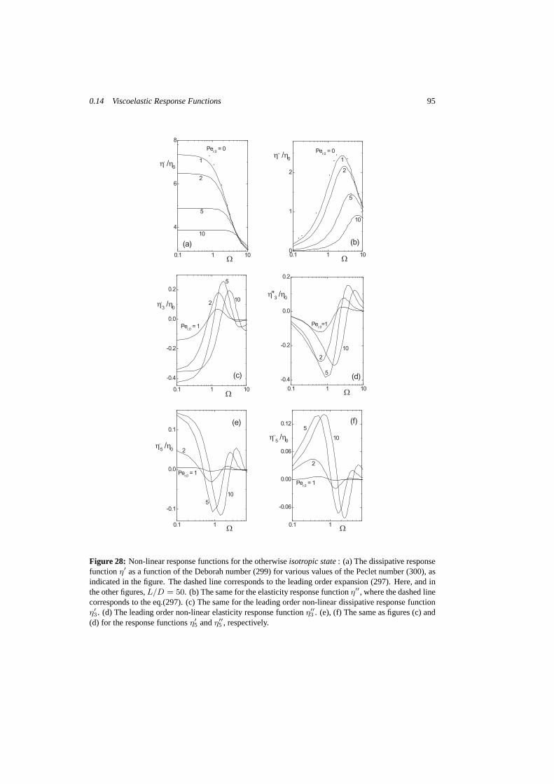
0.14 Viscoelastic Response Functions 95
0.1 1 10
4
6
8
(a)
2
10
5
1
Per,0
= 0
h,/h
0
W0.1 1 100
1
2 2
(b)
10
5
1
Per,0
= 0h
,,/h
0
W
0.1 1 10
-0.4
-0.2
0.0
0.2
(c)
2
Per,0
= 1
5
10h
,
3/h
0
W
0.1 1
-0.1
0.0
0.1(e)
2
Per,0
= 1
5
10
h,
5/h
0
W0.1 1
-0.06
0.00
0.06
0.12 (f)
2
Per,0
= 1
5
10h,,
5/h
0
W
0.1 1 10
-0.4
-0.2
0.0
0.2
h''3/h
0
W
Per,0
=1
2
5
10
(d)
Figure 28: Non-linear response functions for the otherwiseisotropic state: (a) The dissipative responsefunctionη′ as a function of the Deborah number (299) for various values of the Peclet number (300), asindicated in the figure. The dashed line corresponds to the leading order expansion (297). Here, and inthe other figures,L/D = 50. (b) The same for the elasticity response functionη′′, where the dashed linecorresponds to the eq.(297). (c) The same for the leading order non-linear dissipative response functionη′3. (d) The leading order non-linear elasticity response function η′′
3 . (e), (f) The same as figures (c) and(d) for the response functionsη′
5 andη′′5 , respectively.
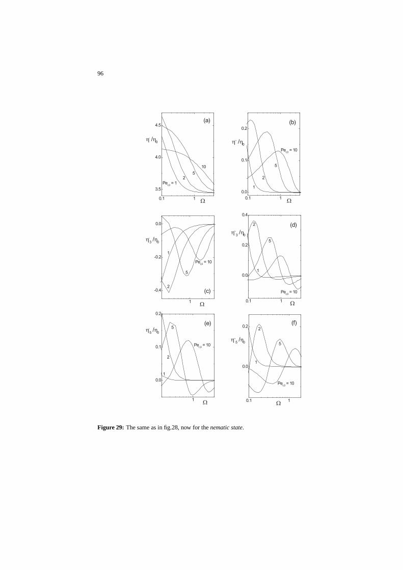
96
0.1 1
3.5
4.0
4.5
10
(a)
2Pe
r,0= 1
5
h,/h
0
W0.1 1
0.0
0.1
0.2
1
2
(b)
Per,0
= 10
5
h,,/h
0
W
1
-0.4
-0.2
0.0
1
(c)2
Per,0
= 10
5
h,
3/h
0
W0.1 1
0.0
0.2
0.4
1
(d)2
Per,0
= 10
5
h,,
3/h
0
W
1
0.0
0.1
0.2
1
(e)
2
Per,0
= 10
5h
,
5/h
0
W 0.1 1
0.0
0.2
1
(f)2
Per,0
= 10
5h
,,
5/h
0
W
Figure 29: The same as in fig.28, now for thenematic state.

0.14 Viscoelastic Response Functions 97
0 3 60
2
4
6
heff
[mPa.s]
c / c*
(b)
0 5 10 150.0
0.5
1.0
pe=10
pe=20
pe=50h
eff/h
0-1
f [%]
(a)
Figure 30: (a) Brownian dynamics simulation data from Claeys et al. (1993) for the suspension shearviscosity (at zero shear-rate and infinite frequency) of ellipsoidal rods as a function of their volumefraction for various aspect ratiospe, as indicated in the figure. (b) Linear concentration dependence ofthe shear viscosity as found in simulations by Yamane et al. (1994).
and ellipsoids, when their lengths are taken equal. In the above we have chosen equal vol-ume fraction and number density of the cylindrical and ellipsoidal rods. This implies equalvolumes of the rods, from which a relation between the thickness of the rods follows as,
De/D =√
3/2 . (305)
Other choices for mapping results for ellipsoidal rods ontothose for cylindrical rods can beused. The above mapping is simple, and correctly compares not only viscosity coefficients butalso diffusion coefficients.
The leading shear thinning behaviour of the zero frequency shear viscosity as found ineq.(291) may be compared to the result obtained by Berry and Russel (1987), which reads inour notation,
ηeff = η0
[
1 +
1 − 1
50
(
γ
Dr
)2
α ϕ +2
5
1 − 0.0342
(
γ
Dr
)2
α2 ϕ2
]
. (306)
up to second order in concentration and shear-rate. This result is valid in the dilute regime,where
`
LD
´2ϕ ≪ 1. To first order in volume fraction this agrees with our result(291). There
are serious differences, however, for theϕ2-contribution. First of all, as discussed in theprevious section, we predict a linear volume fraction dependence of the shear viscosity at zeroshear-rate. From eqs.(290), and from eq.(297) at infinite frequency, we obtain,
ηeff = η0 [ 1 + α ϕ ] , ηeff∞ = η0 [ 1 + 1
4α ϕ ] , (307)
where, as before,ηeff is the zero frequency andηeff∞ the high frequency viscosity. The above
result (306) for zero frequency of Berry and Russel predictson the other hand, at zero-shear-
98
rates and up to second order in concentration,
ηeff = η0
[
1 + α ϕ +2
5α2 ϕ2
]
. (308)
On the basis of this latter prediction, a pronouncedϕ2-dependence for long and thin rods isexpected, sinceαϕ ∼ L
D/ ln L
D → ∞ as L
D→ ∞, for a given value ofL
Dϕ. For zero shear-
rates, we may compare the above predictions with computer simulations by Claeys and Brady(1993) on ellipsoidal rods. In fig.30a, simulation data fromClaeys and Brady (1993) for theeffective zero shear-rate viscosities at infinite frequencies are plotted for three aspect ratiospe
of the ellipsoidal rods :pe = 50, 20 and10. There is a remarkable linear concentration de-pendence over a large concentration range, especially for the longer rods. In fact, Claeys andBrady (1993) remark that “Somewhat surprisingly, the dispersion containing1% rods of as-pect ratio50 still responds hydrodynamically as if it were dilute, even thoughnφ
43πa3 = 25”
(in their notation,nφ is the number density of rods anda = L/2). Such a linear concentrationdependence is also found in computer simulations on non-Brownian rods by et al. (1994) (seefig.30b). They state that “· · · the excess viscosity is proportional to the number densityn evenin the regionnL3 ≈ 40, · · · ”. The magnitude of the second order in volume fraction contribu-tion in the Berry-Russel equation (306), relative to the first order contribution is2
5αϕ ≈ 50%
for the highest concentration shown in fig.30 for bothpe = 20 and50. The large second orderin concentration contributions predicted by Berry and Russel are thus in disagreement withthe linear relationship found in fig.30. A decrease of the Huggins coefficient with increasingaspect ratio is confirmed in experiments on spindle-type colloidal hematite rods by Solomonand Boger (1998) (see fig.2 and table III in this reference).
The slope of the simulation results for the high frequency viscosityηeff∞ versus the volume
fraction in fig.30, taken from Claeys and Brady (1993), may becompared to the slopeα/4as predicted in eq.(307). Noting that the volume fraction ofellipsoids in fig.30a is equal toπ6
DL2 ρ while for the cylindrical particles under consideration here the volume fraction isequal toπ
4DL2 ρ, a slope of36 is found from the simulation data forL/D = 50, whereas
from eq.(289) we find a slope of 29. ForL/D = 20 one finds a slope of9 from fig.30,while α/4 = 6, and forL/D = 10 one finds3.8 andα/4 = 1.9. The slope found fromsimulations thus seems to converge to the asymptotic resultin eq.(307) when the aspect ratiois large enough.
The linear concentration dependence of the zero-shear viscosity is not found within theDEK-theory (Doi and Edwards (1986)), where the concentration dependence originates fromthe assumed state dependence of the rotational tracer diffusion coefficient.
The experiments by Graf et al. (1993) and Schmidt et al. (2000) on fd-virus suspensionsdo not show a linear concentration dependence of the zero-shear and zero-frequency viscosity(except maybe for the salt free case in fig.3 of Graf et al. (1993), which result should not betaken as proof of the present theory in view of the not well understood behaviour of fd-virusat very low ionic strength). The higher order concentrationdependence as found for fd-virus,however, is much weaker than for hard-spheres, indicating that, in accordance with our find-ings, elongated objects tend to diminish non-linear concentration dependence. Similarly, aconsiderable second order concentration dependence of theshear viscosity is found experi-mentally for Xanthan gum by Chauveteau (1982). It is known that fd-virus is relatively stiff(contour length is880 nm, intrinsic persistence length is2200 nm), but nevertheless behaves
0.14 Viscoelastic Response Functions 99
quite non-Onsager like, in the sense that the relative isotropic-nematic bi-phasic gapwidthin the absence of shear flow is much narrower than the width forvery long and thin, truelyrigid rods (see Tang and Fraden (1995)). Hence, even for relatively stiff rod like particles, theapproximation (208) for the pair-correlation function is not very good. Xanthan and “stiff”polymers like PBLG (Yang (1987) and Mead and Larson (1990)),are even more flexible thanfd-virus. The non-zero Huggins coefficient at zero shear-rate found experimentally for fd-virus by Graf et al. (1993), Xanthan gum by Chauveteau (1982)and PBLG by Yang (1987)and Mead and Larson (1990) is probably due to flexibility. In view of this sensitivity onflexibility, it would be very interesting to include flexibility (even up to leading order in theinverse persistence length) in stress calculations. The sensitivity on slight flexibility obscuresthe comparison of theories for truly stiff rods with experiments.
The difference between the experimental rods mentioned above and the model rods incomputer simulations, is their degree of stiffness. The advantage of computer simulations isthat the persistence length of rods can be made infinite. In the computer simulations mentionedabove, hydrodynamics are taken into account. The differentconcentration dependence of thezero shear viscosity (at least for long and thin rods) found in experiments as compared tosimulations, as far as the Huggins coefficient is concerned,is therefore most likely due toflexibility.
Despite the sensitivity of viscoelastic response functions on flexibility, we shall neverthe-less compare experimental data with our theoretical predictions. This comparison should betaken seriously only on a qualitative level. Fig.31 shows experimental data for the shear-ratedependence of the shear viscosity of Xanthan (Chauveteau (1982)) with two different molarweights, PBLG (Yang (1987)) and a salt free fd-virus suspension (Graf et al. (1993)). Plottedis the intrinsic viscosity[η] = η/η0 − 1, with η0 the solvent shear viscosity, relative to itsvalue[η]0 at zero shear-rate. For Xanthan we tookDr = 133 s−1 and103 s−1 for the low andhigh molecular weight, respectively, as reported by Berry and Russel (1987), for PBLG wetookDr = 167 s−1, as reported by Larson (1999), and for salt free fd we tookDr = 11 s−1
(see Graf et al. (1993)). The solid lines refer to the presenttheory withL/D = 50 (the preciseform of these curves is insensitive to the aspect ratio). TheXanthan and PBLG suspensionsare dilute, and are seen to be in reasonable agreement with theory. The concentration of thesalt free fd-virus suspension is equal to6 c∗, wherec∗ is the overlap concentration. There issome deviation from the fd-data in comparison to theory, which may be either due to flexibilityor aggregation at low ionic strength.
The linear concentration dependence in eq.(307) holds up tothe isotropic-nematic phasetransition. Within the nematic state this result is no longer valid, since in deriving eq.(307)we linearized around the isotropic state (see eq.(285)). Ascan be seen from fig.26b, theviscosity decreases with increasing concentration for a nematic. As was mentioned before,this is the result of an increase in alignment on increasing the concentration. Such a decreaseof the shear viscosity with increasing concentration is indeed observed experimentally (see forexample fig.10.5 in Doi and Edwards (1986) and fig.1 in Kiss andPorter (1978)). Furthermore,the type of concentration dependence of the shear viscosityat higher shear-rates as found infig.26c is also seen in experiments (see for example fig.10.9 in Doi and Edwards (1986)).
To leading order in concentration, the low shear limiting expressions (292) for normalstress differences are also found by Hinch and Leal (1972), except that instead of the prefactor
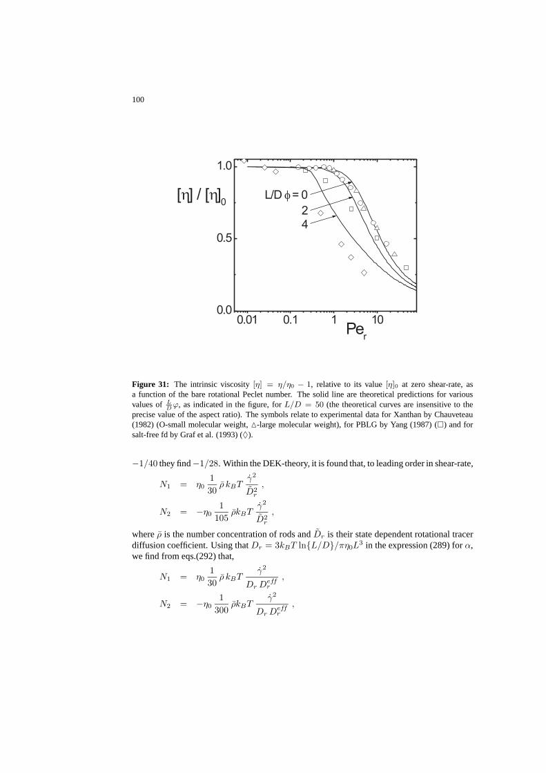
100
0.01 0.1 1 100.0
0.5
1.0
42
L/D f= 0[h] / [h]0
Per
Figure 31: The intrinsic viscosity[η] = η/η0 − 1, relative to its value[η]0 at zero shear-rate, asa function of the bare rotational Peclet number. The solid line are theoretical predictions for variousvalues of L
Dϕ, as indicated in the figure, forL/D = 50 (the theoretical curves are insensitive to the
precise value of the aspect ratio). The symbols relate to experimental data for Xanthan by Chauveteau(1982) (O-small molecular weight,-large molecular weight), for PBLG by Yang (1987) () and forsalt-free fd by Graf et al. (1993) (♦).
−1/40 they find−1/28. Within the DEK-theory, it is found that, to leading order inshear-rate,
N1 = η01
30ρ kBT
γ2
D2r
,
N2 = −η01
105ρkBT
γ2
D2r
,
whereρ is the number concentration of rods andDr is their state dependent rotational tracerdiffusion coefficient. Using thatDr = 3kBT lnL/D/πη0L
3 in the expression (289) forα,we find from eqs.(292) that,
N1 = η01
30ρ kBT
γ2
Dr Deffr
,
N2 = −η01
300ρkBT
γ2
Dr Deffr
,

0.14 Viscoelastic Response Functions 101
where the effective rotational, collective diffusion coefficient Deff is given in eq.(230). Theprefactor forN2 is almost a factor of3 smaller than in the DEK-theory, and in both expres-sions we find the combinationDr Deff
r instead ofD2r . Experimental results for normal stress
differences on fibers are reported by Zirnsak et al. (1994). Here, Brownian motion is veryweak as compared to shear forces, so that one should compare with the high shear-rate resultsas plotted in fig.27. One should be careful in comparing, since inertial effects in fiber suspen-sions may play a role. As can be seen from figs.27a,b, both normal stress differences becomelinear functions of the shear-rate for high shear-rates (sinceN1/γ andN2/γ tend to constant,shear-rate independent values). This remarkable linear shear-rate dependence is indeed typ-ically found in experiments on fibers (see, for example, fig.11 in Zirnsak et al. (1994)). Inaddition, in figs.16,17 of the same reference, it is found that the first normal stress differencevaries linearly with concentration. This is also found in our fig.27e for high shear-rates, forconcentrations whereL
Dϕ is less than about3. The concentrations in the experiments on fibers
is indeed well within this range.
Normal stress differences that change from being positive to negative on increasing theshear-rate, and for larger shear-rates from negative to positive again, were reported by Iizuka(1978), Kiss and Porter (1978), Kiss (1996) and Larson (1996) for PBLG solutions in m-cresol, and later for the same polymer by Magda et al. (1991).Marrucci and Maffettone(1989) predict, on the basis of a two-dimensional DEK-like approach for a homogeneousnematic, that the normal stress differenceN1 is negative at low shear-rates and becomes pos-itive at higher shear-rates (see their fig.10). This behaviour is found for shear-rates which arelarge enough to assure that stationary solutions of equations of motion exist, that is, wheretumbling or wagging are absent. Larson (1990) analyzed the full 3-dimensional DEK-theory(using closures as obtained by Hinch and Leal (1976)), and suggests that the experimentallyobserved sign changes of normal stress differences are due to the existence of tumbling orwagging nematic domains. By time-averaging of stresses generated by tumbling domainsover a number of oscillations, he indeed finds the kind of signchanges for normal stress dif-ferences that are observed experimentally. This kind of behaviour is essentially also foundwithin the two-dimensional DEK-like approach by Marrucci and Maffettone (1990a), Mar-rucci and Maffettone (1990b). Magda et al. (1991) suggestedthat polydomain nematics mayexhibit apparent steady flow behaviour, even though each individual domain exhibits tum-bling or wagging, since in a rheometer averages over many independent tumbling domains areprobed. Tumbling and wagging can be observed in an experiments by flow reversal, whichrenders the various domains coherently tumbling/wagging for some time. As mentioned be-fore, whether a theory predicts tumbling and wagging is verysensitive to the closure relationthat is used. Our closure relation (227) is not suited to describe tumbling and wagging. Otherclosure relations can be used to study these time-periodic states (see Marrucci and Maffettone(1989), Larson (1990), Marrucci and Maffettone (1990a), Marrucci and Maffettone (1990b)and Forest and Wang (2003)). Due to the sensitivity for the prediction of time-periodic stateson the closure relation, the most sensible thing to do seems to employ the original equation ofmotion (213), before introducing a Ginzburg-Landau expansion.

102
Figure 32: A photograph from the side of an optical couette cell betweentwo crossed polarizers. Thecouette cell contains an fd-virus suspensions in a vorticity banded state. The width of the shear cell isabout5 cm, while the height of the bands is about1 mm.
0.15 Current Research Topics
Some of the current research interests related to what has discussed in the present chapter willbe briefly described in this last section. Current research interests include,
(i) shear-banding transitions,
(ii) the non-equilibrium phase behaviour under shear flow,
and,
(iii) phase separation kinetics under flow conditions.
0.15.1 Shear-banding transitions
There are essentially two types of banding transitions observed experimentally in various typesof systems containing mesoscopic entities : vorticity banding and gradient banding. Here,“bands” refer to coexisting regions under stationary flow which have different microstruc-tural order and can sustain different shear rates and/or stresses. In case of vorticity banding,regularly stacked bands in the vorticity direction are observed, which differ in their averageorientational order. For gradient banding, two regions coexists, extending along the gradientdirection, each with a different shear rate.
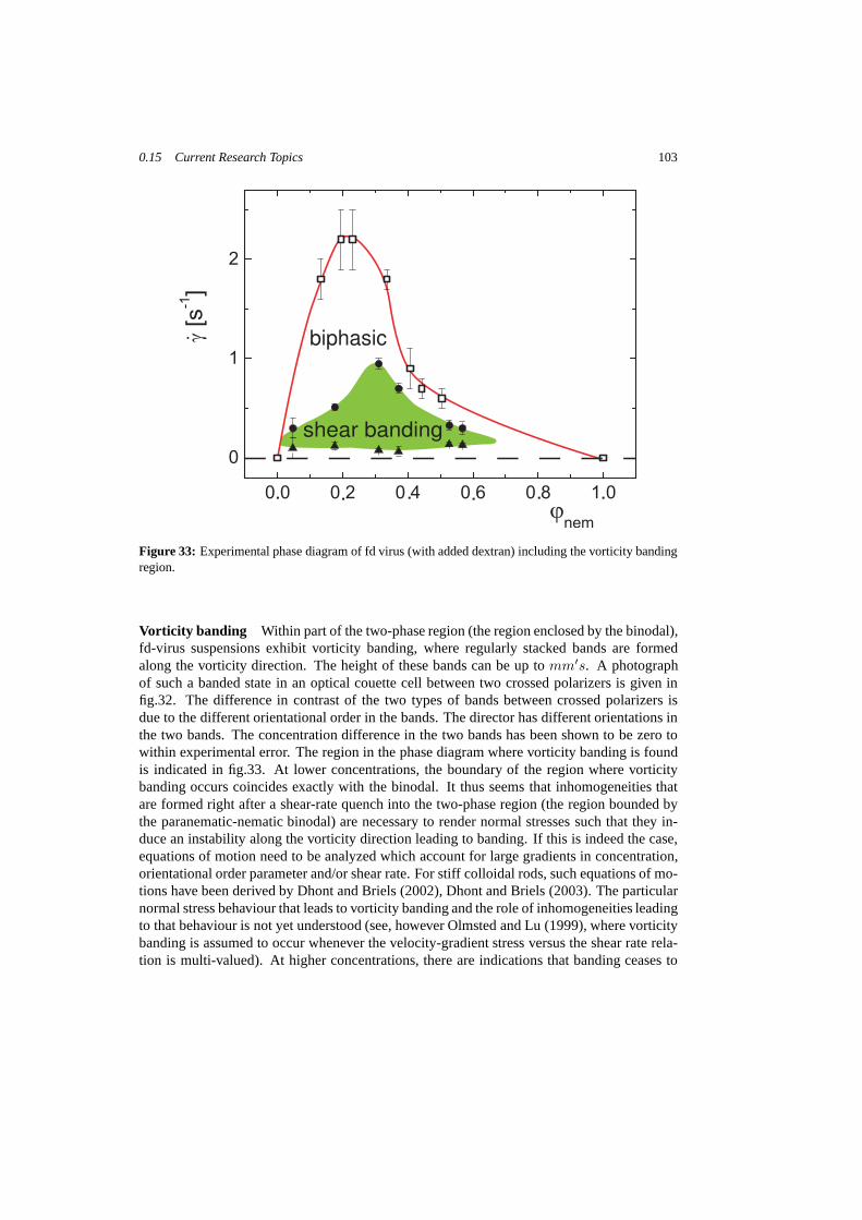
0.15 Current Research Topics 103
.
. .....
biphasic
shear banding
Figure 33: Experimental phase diagram of fd virus (with added dextran)including the vorticity bandingregion.
Vorticity banding Within part of the two-phase region (the region enclosed by the binodal),fd-virus suspensions exhibit vorticity banding, where regularly stacked bands are formedalong the vorticity direction. The height of these bands canbe up tomm′s. A photographof such a banded state in an optical couette cell between two crossed polarizers is given infig.32. The difference in contrast of the two types of bands between crossed polarizers isdue to the different orientational order in the bands. The director has different orientations inthe two bands. The concentration difference in the two bandshas been shown to be zero towithin experimental error. The region in the phase diagram where vorticity banding is foundis indicated in fig.33. At lower concentrations, the boundary of the region where vorticitybanding occurs coincides exactly with the binodal. It thus seems that inhomogeneities thatare formed right after a shear-rate quench into the two-phase region (the region bounded bythe paranematic-nematic binodal) are necessary to render normal stresses such that they in-duce an instability along the vorticity direction leading to banding. If this is indeed the case,equations of motion need to be analyzed which account for large gradients in concentration,orientational order parameter and/or shear rate. For stiffcolloidal rods, such equations of mo-tions have been derived by Dhont and Briels (2002), Dhont andBriels (2003). The particularnormal stress behaviour that leads to vorticity banding andthe role of inhomogeneities leadingto that behaviour is not yet understood (see, however Olmsted and Lu (1999), where vorticitybanding is assumed to occur whenever the velocity-gradientstress versus the shear rate rela-tion is multi-valued). At higher concentrations, there areindications that banding ceases to

104
0.10 0.15 0.20 0.251.0
1.5
2.0
4.28
L/Df = 4.2
s12
Per
0.15 0.16 0.170.65
0.66
0.67
0.68
0.10 0.15 0.20 0.251.0
1.5
2.0
4.28
L/Df = 4.2
s12
Per
0.15 0.16 0.170.65
0.66
0.67
0.68
Figure 34: The dimensionless flow-gradient componentσ12 ≡ Σ12/η0 Dr of the stress tensor as afunction of the shear-rate for concentrations close to the critical concentrationL
Dϕ = 4.281 · · · ; see
fig.19b. The smaller figure on the right side is a blow-up of thevan der Waals loop.
occur when tumbling/wagging sets in.
Gradient banding On the basis of the stationary forms of the equation of motion(219) andthe expression (284) for the deviatoric stress tensor (where Dr is the bare, state-independentrotational diffusion coefficient), a non-monotonic behaviour of the shear-stress as a function ofshear-rate is found. Such a “van der Waals loop-like” behaviour is only found for concentra-tions very close to the critical concentrationL
Dϕ = 4.281 · · · , as can be seen in fig.34, where
the dimensionless flow-gradient componentσ12 = Σ12/η0 Dr of the stress tensor is plottedas a function of shear-rate. Such a decrease of the stress in acertain shear-rate interval impliesthat the usual linear flow profile as depicted in fig.1a is unstable. The stable flow profile is nowa banded flow, where two regions with different shear rates are in coexistence. Within thesetwo regions (the “bands”), the shear rate is constant, independent of position. The shear rateswithin the two bands can be found from a modified equal area construction on the van derWaals loop in fig.34 (see Olmsted and Lu (1999), Olmsted (1999), Olmsted et al. (2000), Luet al. (2000), Fielding and Olmsted (2003) and Dhont (1999)). As can be seen, the differencebetween these shear rates is very small. Since the concentration range where gradient bandingis expected to occur and the difference in shear rates as sustained in the two bands is verysmall, gradient banding in suspensions of stiff rods will bedifficult to detect experimentally.In addition, passing the critical point at a fixed concentration by increasing the shear rate, the
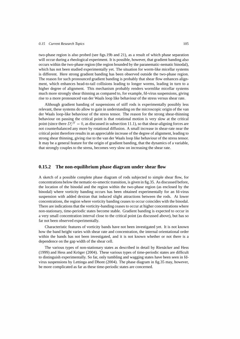
0.15 Current Research Topics 105
two-phase region is also probed (see figs.19b and 21), as a result of which phase separationwill occur during a rheological experiment. It is possible,however, that gradient banding alsooccurs within the two-phase region (the region bounded by the paranematic-nematic binodal),which has not been studied experimentally yet. The situation for worm-like micellar systemsis different. Here strong gradient banding has been observed outside the two-phase region.The reason for such pronounced gradient banding is probablythat shear flow enhances align-ment, which enhances head-to-tail collisions leading to longer worms, leading in turn to ahigher degree of alignment. This mechanism probably renders wormlike micellar systemsmuch more strongly shear thinning as compared to, for example, fd-virus suspensions, givingrise to a more pronounced van der Waals loop like behaviour ofthe stress versus shear rate.
Although gradient banding of suspensions of stiff rods is experimentally possibly lessrelevant, these systems do allow to gain in understanding onthe microscopic origin of the vander Waals loop-like behaviour of the stress tensor. The reason for the strong shear-thinningbehaviour on passing the critical point is that rotational motion is very slow at the criticalpoint (since thereDeff
r = 0, as discussed in subsection 11.1), so that shear-aligning forces arenot counterbalanced any more by rotational diffusion. A small increase in shear-rate near thecritical point therefore results in an appreciable increase of the degree of alignment, leading tostrong shear thinning, giving rise to the van der Waals loop like behaviour of the stress tensor.It may be a general feature for the origin of gradient banding, that the dynamics of a variable,that strongly couples to the stress, becomes very slow on increasing the shear rate.
0.15.2 The non-equilibrium phase diagram under shear flow
A sketch of a possible complete phase diagram of rods subjected to simple shear flow, forconcentrations below the nematic-to-smectic transition,is given in fig.35. As discussed before,the location of the binodal and the region within the two-phase region (as enclosed by thebinodal) where vorticity banding occurs has been obtained experimentally for an fd-virussuspension with added dextran that induced slight attractions between the rods. At lowerconcentrations, the region where vorticity banding ceasesto occur coincides with the binodal.There are indications that the vorticity-banding ceases tooccur at higher concentrations wherenon-stationary, time-periodic states become stable. Gradient banding is expected to occur ina very small concentration interval close to the critical point (as discussed above), but has sofar not been observed experimentally.
Characteristic features of vorticity bands have not been investigated yet. It is not knownhow the band height varies with shear rate and concentration, the internal orientational orderwithin the bands has not been investigated, and it is not known whether or not there is adependence on the gap width of the shear cell.
The various types of non-stationary states as described in detail by Rienacker and Hess(1999) and Hess and Kroger (2004). These various types of time-periodic states are difficultto distinguish experimentally. So far, only tumbling and wagging states have been seen in fd-virus suspensions by Lettinga and Dhont (2004). The phase diagram in fig.35 may, however,be more complicated as far as these time-periodic states areconcerned.
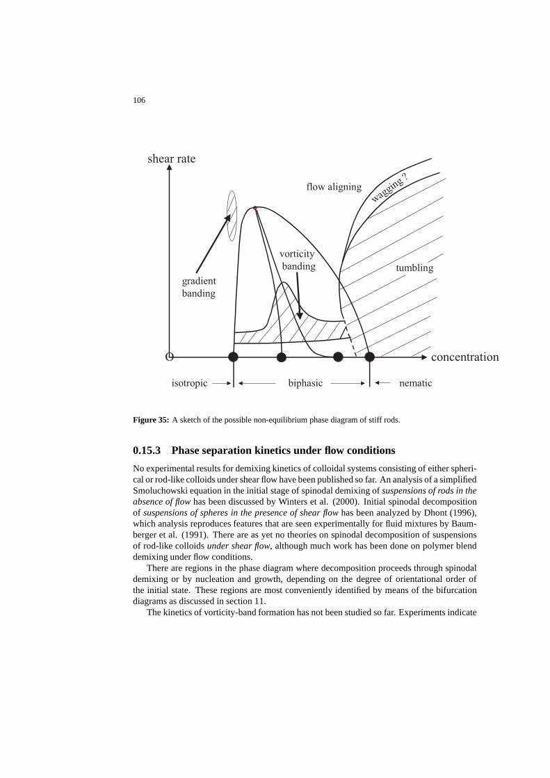
106
concentration
shear rate
O
biphasicisotropic nematic
tumbling
waggin
g ?flow aligning
gradient
banding
vorticity
banding
Figure 35: A sketch of the possible non-equilibrium phase diagram of stiff rods.
0.15.3 Phase separation kinetics under flow conditions
No experimental results for demixing kinetics of colloidalsystems consisting of either spheri-cal or rod-like colloids under shear flow have been publishedso far. An analysis of a simplifiedSmoluchowski equation in the initial stage of spinodal demixing of suspensions of rods in theabsence of flowhas been discussed by Winters et al. (2000). Initial spinodal decompositionof suspensions of spheres in the presence of shear flowhas been analyzed by Dhont (1996),which analysis reproduces features that are seen experimentally for fluid mixtures by Baum-berger et al. (1991). There are as yet no theories on spinodaldecomposition of suspensionsof rod-like colloidsunder shear flow, although much work has been done on polymer blenddemixing under flow conditions.
There are regions in the phase diagram where decomposition proceeds through spinodaldemixing or by nucleation and growth, depending on the degree of orientational order ofthe initial state. These regions are most conveniently identified by means of the bifurcationdiagrams as discussed in section 11.
The kinetics of vorticity-band formation has not been studied so far. Experiments indicate
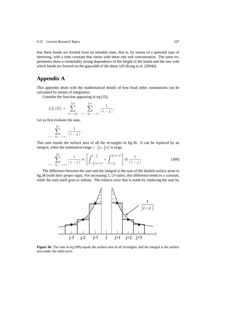
0.15 Current Research Topics 107
that these bands are formed from an unstable state, that is, by means of a spinodal type ofdemixing, with a time constant that varies with shear rate and concentration. The same ex-periments show a remarkably strong dependence of the heightof the bands and the rate withwhich bands are formed on the gapwidth of the shear cell (Kanget al. (2004)).
Appendix A
This appendix deals with the mathematical details of how bead index summations can becalculated by means of integration.
Consider the function appearing in eq.(35),
f(L/D) =
12n∑
j=− 12n
12 n∑
i = − 12
n , i 6= j
1
| i − j | .
Let us first evaluate the sum,12n∑
i = − 12
n , i 6= j
1
| i − j | .
This sum equals the surface area of all the rectangles in fig.36. It can be replaced by anintegral, when the summation range(− 1
2n, 12n) is large,
12n∑
i = − 12
n , i 6= j
1
| i − j | ≈[
∫ j− 12
− 12 (n+1)
+
∫ 12 (n+1)
j+ 12
]
di1
| i − j | . (309)
The difference between the sum and the integral is the sum of the dashed surface areas infig.36 (with their proper sign). For increasingL/D-ratios, this difference tends to a constant,while the sum itself goes to infinity. The relative error thatis made by replacing the sum by
ij j+1 j+2 j+3j-1j-2j-3
ji -
1
ij j+1 j+2 j+3j-1j-2j-3
ji -
1
Figure 36: The sum in eq.(309) equals the surface area of all rectangles, and the integral is the surfacearea under the solid curve.

108
an integral thus tends to zero asL/D tends to infinity. The leading terms in the above integralare,
lnj +1
2(n + 1) + ln1
2(n + 1) − j .
This expression is substituted into eq.(309), where the sumover j is again replaced by anintegral. Using the standard integral,
∫
dz zm lnz = zm+1
[
lnzm + 1
− 1
(m + 1)2
]
,
one ends up, to leading order inD/L, with the result given in eq.(36). The two values ofj = ±n/2 do not contribute to leading order, so that in the evaluationof summations,j mayalways be assumed in the interior of the summation range.
Appendix B : Useful mathematical identities
Useful mathematical identities which are frequently used in the present chapter are,
R2(· · · ) = −2u · ∇u(· · · ) − uu : ∇u∇u(· · · ) + ∇2
u(· · · ) ,
R2(a · u)2 = 2
[
a2 − 3(a · u)2]
,
R2(u ·M · u) = −6 (u · M · u) + 2 TrM ,
R2(uu) = −6uu + 2I ,
(u× M · u) · R(· · · ) = [∇u(· · · )]·(M·u)−(u·[∇u(· · · )])(u·M·u) ,
R · [u × (M · u)] = −3(u · M · u) + TrM ,
R · ((· · · )(u · M · u)) = [TrM − 3(u ·M · u)] (· · · ) + (M · u) ·[
I − uu]
· ∇u(· · · ) ,
R · (u× a) = −2(u · a) ,
R(u ·M · u) = u×[
M · u + MT · u]
,
a · Ru = a× u .
Here,M anda denoteu-independent tensor and vector, respectively, and(· · · ) denotes anarbitrary, but differentiable, scalar or vector field. The above identities are easily verified byexplicit differentiation.
Appendix C : On the accuracy of the closure relation (227)
In order to asses the accuracy of the closure relation (227),we numerically solve the Smolu-chowski equation (213) for a single rod in shear flow, that is,without the interaction term.From the stationary numerical solutionP (u, t → ∞), bothS andS(4) can be obtained bynumerical integration. This allows to compare the approximation (227) with the exact form ofS(4). Note that the stationary solution of eq.(213) is a functionof the shear rate through thedimensionless rotational Peclet numberPer = γ/Dr.
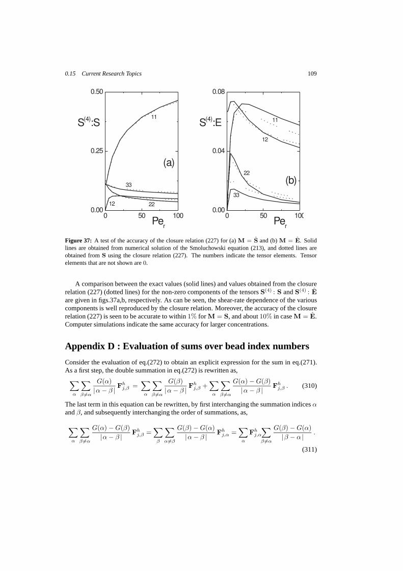
0.15 Current Research Topics 109
0 50 1000.00
0.25
0.50
(a)
33
2212
11
S(4)
:S
Per
0 50 1000.00
0.04
0.08
(b)
33
22
12
11S(4)
:E
Per
Figure 37: A test of the accuracy of the closure relation (227) for (a)M = S and (b)M = E. Solidlines are obtained from numerical solution of the Smoluchowski equation (213), and dotted lines areobtained fromS using the closure relation (227). The numbers indicate the tensor elements. Tensorelements that are not shown are0.
A comparison between the exact values (solid lines) and values obtained from the closurerelation (227) (dotted lines) for the non-zero components of the tensorsS(4) : S andS(4) : E
are given in figs.37a,b, respectively. As can be seen, the shear-rate dependence of the variouscomponents is well reproduced by the closure relation. Moreover, the accuracy of the closurerelation (227) is seen to be accurate to within1% for M = S, and about10% in caseM = E.Computer simulations indicate the same accuracy for largerconcentrations.
Appendix D : Evaluation of sums over bead index numbers
Consider the evaluation of eq.(272) to obtain an explicit expression for the sum in eq.(271).As a first step, the double summation in eq.(272) is rewrittenas,
∑
α
∑
β 6=α
G(α)
|α − β | Fhj,β =
∑
α
∑
β 6=α
G(β)
|α − β | Fhj,β +
∑
α
∑
β 6=α
G(α) − G(β)
|α − β | Fhj,β . (310)
The last term in this equation can be rewritten, by first interchanging the summation indicesαandβ, and subsequently interchanging the order of summations, as,
∑
α
∑
β 6=α
G(α) − G(β)
|α − β | Fhj,β =
∑
β
∑
α6=β
G(β) − G(α)
|α − β | Fhj,α =
∑
α
Fhj,α
∑
β 6=α
G(β) − G(α)
|β − α | .
(311)

110
After a similar interchange of the order of summation in the first term on the right hand-sideof eq.(310), substitution of eqs.(310,311) into eq.(272) gives,
∑
α
G(α)Fhj,α = −γ
∑
α
G(α) [vj,α − Uj,α]− 38
[
I + ujuj
]
·
∑
α
G(α)Fhj,α
∑
β 6=α
1
|α − β | + ∆
,
(312)
where,
∆ =∑
α
Fhj,α
∑
β 6=α
G(β) − G(α)
|β − α | . (313)
Consider the first contribution between the square bracketsin eq.(312),∑
α
G(α)Fhα
∑
β 6=α
1
|α − β | . (314)
The sumS(α) ≡ ∑
β 6=α 1/ |α− β | can be approximated by an integral. To leading order onefinds,
S(α) ≡∑
β 6=α
1
|α − β | =
[
∫ α− 12
− 12 ( L
D−1)
+
∫ 12 ( L
D−1)
α+ 12
]
dx1
|x − β | .
The integrals are easily evaluated to yield,
S(α) = 2 ln2 + ln 12( L
D− 1) + α + ln 1
2( L
D− 1) − α .
Except forα’s close to the ends of the rod, this gives to leading order,
S(α) ≈ 2 ln LD . (315)
In fig.38a,S(α)/2 lnL/D is plotted as a function ofα/m, with 2m + 1 the number ofbeads (so thatα/m ranges from−1 to +1). As can be seen, the approximation (315) is goodto within about10 %, except at the very ends of the rod. In fact, the width of the region atthe tips of the rod where eq.(315) is not a good approximationasymptotically vanishes in thelimit whereL/D → ∞. Hence, except whenG(α)Fh
j,α in eq.(314) peaks at the ends of rodj, eq.(315) can be used as a good approximation. For our purpose, there is no reason for thefunctionG(α)Fh
j,α to peak at the very ends of the rod. A quantitative estimate for the errormade in using eq.(315), is the differences between the sums
∑
α S(α) and∑
α 2 lnL/D =2(L/D − 1) lnL/D. These sums are plotted as functions ofL/D in fig.38b. The relativeerror does not exceed8 % (for L/D ≤ 5), and very slowly converges to0 with increasingaspect ratio. Hence, to within about10 % error, we can approximate the expression in eq.(314)by,
∑
α
G(α)Fhα
∑
β 6=α
1
|α − β | = 2 lnL/D∑
α
G(α)Fhj,α . (316)
The term on the left hand-side in eq.(312) can be neglected against this contribution, which islogarithmically larger.

0.15 Current Research Topics 111
50 100 150 2000
500
1000
1500
2000
2 (L/D-1) ln(L/D)
SaS(a)
(b)Sum
L/D-1.0 -0.5 0.0 0.5 1.0
0.0
0.2
0.4
0.6
0.8
1.0
(a)
S( ) / 2 ln(L/D
201
L/D = 21
/ m
Figure 38: (a) S(α)/2 lnL/D as a function ofα/m with 2m + 1 the total number of beads (whereS(α) ≡
P
β 6=α 1/ | α − β |). The lower curve is forL/D = 20, the upper curve forL/D = 201. (b)the sums
P
α S(α) andP
α 2lnL/D = 2(L/D − 1) lnL/D as a function ofL/D. The relativeerror between the two sums never exceeds8%, and very slowly converges to0 with increasingL/D.
For the divergence of the stress tensor in eq.(267) we need toevaluate the sum,
S ≡∑
α
< δ(r − r1 − α D u1)Fh1,α > .
wherej is taken equal to1 for convenience. Writing the ensemble average in terms of anintegral with respect to the probability density function (pdf)P , of all phase space coordinatesof the colloidal rods, the integration with respect tor1 can be done immediately due to thedelta distribution, leading to,
S =
∮
du1
∫
dΓ∑
α
P (r1 = r − α Du1, u1,Γ, t)Fh1,α(r1 = r − α Du1, u1,Γ),
whereΓ stands for the phase space coordinatesr2, · · · , rN , u2, · · · , uN . The integrand is ofthe form of the left hand-side of eq.(272), except that inFh
1,α the positionr1 is taken equal tor−α Du1, which does not affect the present analysis leading to eq.(273). The functionG(α)is now equal to,
G(α) = P (r1 = r − α Du1, u1,Γ, t) .
Since the pdf is a continuous differentiable function ofr1, there is a scalarz betweenα andβ, such that,
G(β) − G(α)
β − α=
dG(z)
dz≡ dP (r1 = r− z Du1, u1,Γ, t)
dz.
112
The latter derivative is just the change ofP on changing the position of rod number1 byD u1, that is, its center is shifted over a distanceD in the direction of its orientation. Sincefor the very large aspect ratios under consideration, suspension properties are essentiallyconstant over distances of the orderD, so that this is a very small number. The numberR = (L/D)d lnG(z)/dz measures the change of “the entropy”lnP over distances ofthe order of the length of the rods. In terms of this number we have the order of magnitudeestimate,
∆ ∼ R∑
α
G(α)Fh1,α .
Hence, according to eq.(316), as long as relative changes ofsuspension properties over thecontour of the rods are much smaller thanlnL/D, ∆ can be neglected against the first termbetween the square brackets in eq.(312). This justifies the step from eqs.(267) to eq.(273,274).
Appendix E : Derivation of eq.(279)
After substitution of eqs.(278,170,166,172,277) into eq.(275) it is immediately found that,
∇ · Σ = η0∇2U(r, t) −∇P ss(r, t) + Ir + It + Iu , (317)
where,
Ir = − γ D Dr
lnL/D<
N∑
j=1
∑
α
α δ(r − rj − α Duj)[
βRjΨ + Rj lnP]
× uj > , (318)
It = − γ DlnL/D
<
N∑
j=1
∑
α
δ(r − rj − α Duj) [β∇jΨ + ∇j lnP] > , (319)
and,
Iu = 43
γlnL/D
<
N∑
j=1
[
I− 12ujuj
]
·∑
α
δ(r − rj − α Duj)
×
DL
∑
β
Uj,β − Uj,α − 12 α (DL
)3uj × uj ×
∑
β
β Uj,β
> . (320)
First consider the relatively simple contribution,
I ≡ <
N∑
j=1
∑
α
α δ(r − rj − α Duj) uj × Rj lnP >
=
N∑
j=1
∑
α
α
∫
dr1 · · ·∫
drN
∮
du1 · · ·∮
duN δ(r−rj−αDuj) uj × Rj P .
0.15 Current Research Topics 113
that appears in eq.(318) forIr. In the second line it is used thatP Rj lnP = RjP , where,P ≡ P (r1, · · · , uN , t) is theN -particle pdf. For eachj, the integrations with respect torm
andum with m 6= j can be done immediately. Assuming identical rods gives,
I = N∑
α
α
∫
dr1
∮
du1 δ(r−r1−α Du1) u1 × R1 P (r1, u1, t) .
It is to be noted that the differentiation with respect tou1 must be performed, after whichr1
can be replaced byr − αDu1 upon integration with respect tor1. Hence,
I = N∑
α
α
∮
du1 u1 ×[
R1 P (r− α Du0, u1, t)]
u0=u1
.
The corresponding contribution to the divergence of the stress tensor in eq.(279) follows byreplacing the summation over the bead index numberα by an integral as,
∑
α
f(· · · − α Du1) = D−1
∫ L/2
−L/2
dx f(· · · − x u1) . (321)
Next consider the somewhat more complicated contribution,
I ≡ β <N
∑
j=1
∑
α
α δ(r − rj − α Duj) uj × RjΨ >
= β
N∑
j=1
∑
α
α
∫
dr1 · · ·∫
drN
∮
du1 · · ·∮
duN δ(r−rj−α Duj) P uj × RjΨ ,
which appears in eq.(318) forIr. Using pair-wise additivity (see eq.(203)), substitutionofeq.(207) together with eq.(209), and assuming identical rods, it is readily found that,
I =∑
α
α
∫
dr1
∮
du1
∮
du2 δ(r−r1−α Du1) ρ(r1, u1, t)
u1×R1
∫
dr2 ρ(r2, u2, t)χ(r1−r2, u1, u2) . (322)
The integration with respect tor2 can be performed after transforming to the integration vari-ableR = r1 − r2,
∫
dr2 ρ(r2, u2, t)χ(r1−r2, u1, u2) =
∫
dR ρ(r1−R, u2, t)χ(R, u1, u2)
= 2D | u1×u2 |∫ L/2
−L/2
dl
∫ L/2
−L/2
dl′ ρ(r1−l u1−l′ u2, u2, t) .
In the second equation, the integration with respect toR is transformed to integration withrespect tol, l′, l′′, which are defined as, ,
R = l u1 + l′ u2 + l′′u1 × u2
| u1 × u2 |,
− 12L ≤ l , l′ ≤ 1
2L , −D ≤ l′′ ≤ D . (323)
114
The Jacobian of this transformation is equal to| u1 × u2 |. Since the suspension propertiesdo not significantly change over distances of the order of thethicknessD of the rods, theintegration with respect tol′′ gives rise to a prefactor2D. Hence,
I = 2D∑
α
α
∫
dr1
∮
du1
∮
du2
∫ L/2
−L/2
dl
∫ L/2
−L/2
dl′ δ(r−r1−α Du1) ρ(r1, u1, t)
u1×R1 | u1×u2 | ρ(r1−l u1−l′ u2, u2, t) .
As before it should be noted that upon integration with respect to r1, the delta distributionrendersr1 = r − αDu1 after the differentiation with respect tou1 has been performed.Hence,
I = 2D∑
α
α
∮
du1
∮
du2
∫ L/2
−L/2
dl
∫ L/2
−L/2
dl′ ρ(r − α Du1, u1, t)
u1×[
R1 | u1×u2 | ρ(r − α Du0−l u1−l′ u2, u2, t)]
u0=u
.
The bead index summation is replaced by an integral similarly as in eq.(321), leading to (withu = u1 andu
′ = u2),
I = 2D
∮
du
∮
du′
∫ L/2
−L/2
dx
∫ L/2
−L/2
dl
∫ l/2
−L/2
dl′ xρ(r − x, u, t)
u×[
R | u×u′ | ρ(r − x u0 − l u− l′ u′, u, t)
]
u0=u
.
This expression can be found in eq.(279).The contributionIt to the stress tensor in eq.(319) is evaluated similarly.Theβ-summations in the contributionIu in eq.(320) are replaced by integrals, similar to
eq.(321), as,∑
β
β Uj,β = D−2
∫
dx′ x′ U(rj +x′ uj) . (324)
The prefactors in eqs.(318,319,320) are found from eqs.(169,171) to be equal to,
γ D
lnL/D= D
LkBT , and , 4
3γ D Dr
lnL/D= 12D2
L3 kBT .
This concludes the mathematical details leading to eq.(279).

Bibliography
Batchelor, G. K., 1970,J. Fluid Mech.41, 545.
Baumberger, T., Perrot, F., and Beysens, D., 1991,Physica A174, 31.
Berry, D. H. and Russel, W. B., 1987,Fluid Mech.180, 475.
Bolhuis, P. and Frenkel, D., 1997,J. Chem. Phys.106, 666.
Bretherton, F. P., 1962,J. Fluid Mech.14, 284.
Chauveteau, G., 1982,J. Rheol.26, 111.
Claeys, I. L. and Brady, J. F., 1993,Fluid Mech.251, 442.
de la Torre, J. G. and Bloomfield, V. A., 1981,Quarterly Rev. Biophys.14, 81.
Deutch, J. M. and Oppenheim, I. J., 1971,J. Chem. Phys.54, 3547.
Dhont, J. K. G., 1996,An Introduction to Dynamics of Colloids. Elsevier, Amsterdam.
Dhont, J. K. G., 1999,Phys. Rev. E60, 4534.
Dhont, J. K. G. and Briels, W. J., 2002,J. Chem. Phys.117, 3992.
Dhont, J. K. G. and Briels, W. J., 2003,J. Chem. Phys.118, 1466.
Dhont, J. K. G. and Nagele, G., 1998,Phys. Rev. E58, 7710.
Doi, M., 1981,J. Pol. Sci.: Pol. Phys. Edition19, 229.
Doi, M. and Edwards, S. F., 1978a,J. Chem. Soc. Faraday Trans. 274, 560.
Doi, M. and Edwards, S. F., 1978b,J. Chem. Soc. Faraday Trans. 274, 918.
Doi, M. and Edwards, S. M., 1986,The Theory of Polymer Dynamics. Oxford UniversityPress, Oxford.
Doi, M., Shimada, T., and Okano, K., 1988,J. Chem. Phys.88, 4070.
Erpenbeck, J. J. and Kirkwood, J. G., 1963,J. Chem. Phys.38, 1023.
Fielding, S. M. and Olmsted, P. D., 2003,Eur. Phys. J. E11, 65.
Forest, M. G. and Wang, Q., 2003,Rheol. Acta42, 20.
Fraden, S., Maret, G., Caspar, D. L. D., and Meyer, R. B., 1989, Phys. Rev. Lett.63, 2068.
Graf, C., Kramer, H., Deggelmann, M., Hagenbuchle, M., Johner, C., Martin, C., andWeber, R., 1993,J. Chem. Phys.98, 4920.
Grelet, E. and Fraden, S., 2003,Phys. Rev. Lett.90, 198302.
116 BIBLIOGRAPHY
Happel, J. and Brenner, H., 1983,Low Reynolds Number Hydrodynamics. Martinus NijhoffPublishers, The Hague.
Hess, S. and Kroger, M., 2004,J. Phys.: Condensed Matter38, 3835.
Hinch, E. J. and Leal, L. G., 1972,J. Fluid Mech.52, 683.
Hinch, E. J. and Leal, L. G., 1976,J. Fluid Mech.76, 187.
Iizuka, E., 1978,Kiss and Porter (1978) refers to a personal communication with Iizukawho apparently found negative normal stress differences before or at the same time asKiss and Porter (1978), but never published these data..
Ingber, M. S. and Mondy, L. A., 1994,J. Rheol.38, 1829.
Jefferey, G. B., 1922,Proc. R. Soc. London, Ser A102, 161.
Kang, K., Lettinga, M. P., and Dhont, J. K. G., 2004,Unpublished.
Kiss, G., 1996,J. Polym. Sci.: Part B : Polym. Phys.34, 2263.
Kiss, G. and Porter, R. S., 1978,J. Polym. Sci.: Polym. Symp.65, 193.
Kuhn, W. and Kuhn, H., 1945,Helv. Chim. Acta28, 97 (in German).
Kuzuu, N. and Doi, M., 1983,J. Phys. Soc. Japan52, 3486.
Larson, R. G., 1990,Macromolecules23, 3983.
Larson, R. G., 1996,J. Polym. Sci.: Part B : Polym. Phys.34, 2267.
Larson, R. G., 1999,The Structure and Rheology of Complex Fluids. Oxford UniversityPress, NY/Oxford.
Leal, L. G. and Hinch, E. J., 1972,J. Fluid Mech55, 161.
Lenstra, T. A. J., Dogic, Z., and Dhont, J. K. G., 2001,J. Chem. Phys.114, 10151.
Lettinga, M. P. and Dhont, J. K. G., 2004,J. Phys.: Condensed Matter16, 3929.
Lu, C.-Y., Olmsted, P. D., and Ball, R. C., 2000,Phys. Rev. Lett.84, 642.
Magda, J. J., Baek, B. S.-G., de Vries, K. L., and Larson, R. G., 1991,Macromolecules24,4460.
Maier, W. and Saupe, A., 1958,Z. Naturforsch.13A, 564.
Maier, W. and Saupe, A., 1959,Z. Naturforsch.14A, 882.
Maier, W. and Saupe, A., 1960,Z. Naturforsch.15A, 287.
Marrucci, G. and Maffettone, P. L., 1989,Macromolecules22, 4076.
Marrucci, G. and Maffettone, P. L., 1990a,J. Rheol.34, 1217.
Marrucci, G. and Maffettone, P. L., 1990b,J. Rheol.34, 1231.
Mead, D. W. and Larson, R. G., 1990,Macromolecules23, 2524.
Murphy, T. J. and Aquirre, J. L., 1972,J. Chem. Phys.57, 2098.
Olmsted, P. D., 1999,Europhys. Lett.48, 339.
Olmsted, P. D. and Lu, C.-Y. D., 1999,Phys. Rev. E60, 4397.
BIBLIOGRAPHY 117
Olmsted, P. D., Radulescu, O., and Lu, C.-Y. D., 2000,J. Rheol.44, 257.
Onsager, L., 1933,Chem. Rev.13, 73.
Onsager, L., 1942,Phys. Rev.62, 558.
Onsager, L., 1949,Ann. N.Y.Acad.Sci51, 627.
Oseen, C. W., 1927,Neuere Methoden und Ergebnisse in der Hydrodynamik. AkademischeVerlagsgesellschaft, Leipzig.
Papathanasiou, T. D. and Guell, D. C., 1997,Flow-induced alignment in composite mate-rials. Woodhead Publishing Ltd., Cambridge.
Rienacker, G. and Hess, S., 1999,Physica A267, 294.
Russel, W. B., Saville, D. A., and Schowalter, W. R., 1991,Colloidal Dispersions. Cam-bridge University Press, Cambridge.
Schmidt, F. G., Hinner, B., Sackmann, E., and Tang, J. X., 2000, Phys. Rev. E62, 5509.
Shimada, T., Doi, M., and Okano, K., 1988,J. Chem. Phys.88, 7181.
Simha, R., 1940,J. Phys. Chem.44, 25.
Solomon, M. J. and Boger, D. V., 1998,J. Rheol.42, 929.
Strating, P., 1995,J. Chem. Phys.103, 10226.
Tang, J. and Fraden, S., 1993,Phys. Rev. Lett.71, 3509.
Tang, J. and Fraden, S., 1995,Liquid Crystals19, 459.
Tao, Y., den Otter, W. K., Padding, J. P., and Briels, W. J., 2004,unpublished.
Vermant, J., Yang, H., and Fuller, G. G., 2001,AIChE Journal47, 790.
Winkler, R. G. and Gompper, G., 2004,unpublished.
Winkler, R. G., Mussawisade, K., Ripoll, M., and Gompper, G., 2004,J. Phys. Condens.Matter 16, S3941.
Winters, J. W., Odijk, T., and van der Schoot, P., 2000,Phys. Rev. E63, 011501.
Yamamoto, S. and Matsuoka, T., 1995,J. Chem. Phys.102, 2254.
Yamane, Y., Kaneda, Y., and Doi, M., 1994,J. Non-Newtonian Fluid Mech.54, 405.
Yang, J. T., 1987,Dynamics of Polymeric Liquids, vol. 2. John Wiley and Sons, Inc.
Zirnsak, M. A., Hur, D. U., and Boger, D. V., 1994,J. Non-Newtonian Fluid Mech.54, 153.
View publication statsView publication stats