Physics of Complex SystemsBrownian Motion

P.I. HurtadoDepartamento de Electromagnetismo y Física de la Materia, and Instituto Carlos I de Física Teórica yComputacional. Universidad de Granada. E-18071 Granada. SpainE-mail: phurtado@onsager.ugr.es

Abstract. These notes correspond to a short lesson of a course on the Physics of Complex Systems within the Degreeon Physics of University of Granada (4th year). In this chapter we review the phenomenon of Brownian motion, andits description from different points of view.

Keywords: Statistical physics, complex systems, probability and statistics, stochastic differential equations, Langevinequation, Fokker-Planck equation, molecular dynamics.

References and sources

[1] R. Mazo, Brownian Motion: Fluctuations, Dynamics and Applications, Oxford University Press (2002).[2] R. Zwanzig, Nonequilibrium Statistical Mechanics, Oxford University Press (2001).[3] N.G. van Kampen, Stochastic Processes in Physics and Chemestry, Elsevier (2007).[4] R. Toral and P. Collet, Stochastic Numerical Methods, Wiley (2014).[5] P.L. Krapivsky, S. Redner and E. Ben-Naim, A Kinetic View of Statistical Physics, Cambridge University Press (2010).[6] D. Chowdhury, 100 years of Einstein’s Theory of Brownian Motion: from Pollen Grains to Protein Trains -1, Resonance,

September 2005, pp. 63–78.

CONTENTS 2Contents

1 A brief historical perspective on Brownian motion 4

2 Einstein theory 10

3 Langevin theory, Stokes-Einstein relation and Green-Kubo formula 153.1 A simple example of Green-Kubo formula for transport coefficients . . . . . . . . . . . . . . . . . . 17

4 Stochastic differential equations and Fokker-Planck equations 194.1 Stochastic differential equations . . . . . . . . . . . . . . . . . . . . . . . . . . . . . . . . . . . . . 194.2 Fokker-Planck equations . . . . . . . . . . . . . . . . . . . . . . . . . . . . . . . . . . . . . . . . . 21

5 The random walk model 235.1 A glimpse at rare events and large deviations . . . . . . . . . . . . . . . . . . . . . . . . . . . . . . 26

6 Appendix: Derivation of Fokker-Planck equation 296.1 Deterministic dynamics and sampling over initial conditions . . . . . . . . . . . . . . . . . . . . . . 296.2 Full stochastic dynamics . . . . . . . . . . . . . . . . . . . . . . . . . . . . . . . . . . . . . . . . . 32

After a brief historical account, we describe Einstein theory on Brownian motion, which led via Perrin’sexperiment to the verification of the molecular hypothesis. We also describe Langevin’s approach in terms of arandom force, and how the comparison of both approaches leads to Stokes-Einstein relation. Langevin’s theoryallows us to introduce the concept of stochastic differential equations, and its equivalent description in terms ofFokker-Planck equations. Finally, we discuss the Random Walk model as a microscopic approach to Brownianmotion. This last approach allows us to introduce the concept of large deviations and rare event statistics.

CONTENTS 31. A brief historical perspective on Brownian motion

• Brownian motion is the random motion of particles suspended in a fluid(a liquid or a gas).

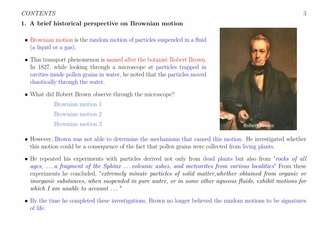
• This transport phenomenon is named after the botanist Robert Brown.In 1827, while looking through a microscope at particles trapped incavities inside pollen grains in water, he noted that the particles movedchaotically through the water.

• What did Robert Brown observe through the microscope?Brownian motion 1Brownian motion 2Brownian motion 3

• However, Brown was not able to determine the mechanisms that caused this motion. He investigated whetherthis motion could be a consequence of the fact that pollen grains were collected from living plants.

• He repeated his experiments with particles derived not only from dead plants but also from "rocks of allages, . . . a fragment of the Sphinx . . . volcanic ashes, and meteorites from various localities" From theseexperiments he concluded, "extremely minute particles of solid matter,whether obtained from organic orinorganic substances, when suspended in pure water, or in some other aqueous fluids, exhibit motions forwhich I am unable to account . . . "

• By the time he completed these investigations, Brown no longer believed the random motions to be signaturesof life.

CONTENTS 4• Following Brown’s work, several other investigators studied Brownian motion in further detail. All theseinvestigations helped in narrowing down the plausible cause(s) of the incessant motion of the Brownian particles.For example, temperature gradients, capillary actions, convection currents, etc. could be ruled out.

• Did Brown really discover the phenomenon which is named after him? No. In fact, Brown himself did not claimto have discovered it. Brownian motion had been observed as early as in the seventeenth century by Antony vanLeeuwenhoek under simple optical microscope. It was reported by Jan Ingenhousz in the eighteenth century. Infact, Brown himself critically reviewed the works of several of his predecessors.

• Even the Roman Lucretius’s scientific poem "On the Nature of Things" (c. 60 BC!!) has a remarkable descriptionof Brownian motion of dust particles in verses 113–140 from Book II. He uses this as a proof of the existence ofatoms:"Observe what happens when sunbeams are admitted into a building and shed light on its shadowy places. You willsee a multitude of tiny particles mingling in a multitude of ways... their dancing is an actual indication of underlyingmovements of matter that are hidden from our sight... It originates with the atoms which move of themselves. . . "

• Nevertheless, this phenomenon was named after Brown; this reminds us of Stiglers law of eponymy:"No scientific discovery is named after its original discoverer".

• But what is the physical origin of this phenomenon? Brownian motion results from the collision of the mesoscopicparticles suspended in a fluid with the fast-moving atoms or molecules in the gas or liquid.

• The direction of the force of atomic bombardment is constantly changing, and at different times the particle is hitmore on one side than another, leading to the seemingly random nature of the motion. A computer simulationmay help in visualizing this phenomenon:

Simulation of Brownian motion

CONTENTS 5

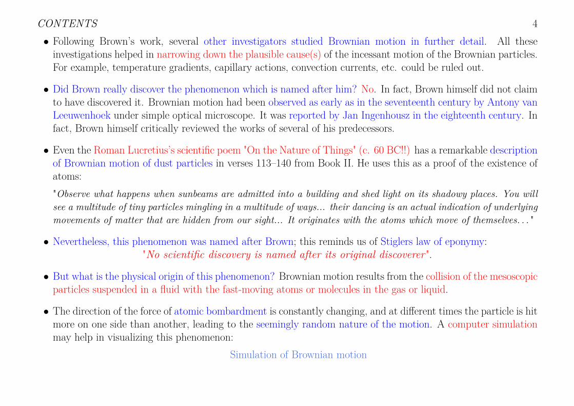
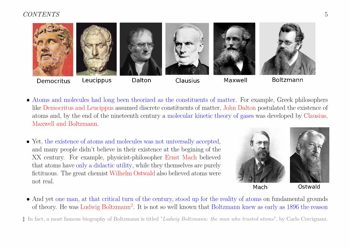
• Atoms and molecules had long been theorized as the constituents of matter. For example, Greek philosopherslike Democritus and Leucippus assumed discrete constituents of matter, John Dalton postulated the existence ofatoms and, by the end of the nineteenth century a molecular kinetic theory of gases was developed by Clausius,Maxwell and Boltzmann.

• Yet, the existence of atoms and molecules was not universally accepted,and many people didn’t believe in their existence at the begining of theXX century. For example, physicist-philosopher Ernst Mach believedthat atoms have only a didactic utility, while they themselves are purelyfictituous. The great chemist Wilhelm Ostwald also believed atoms werenot real.

• And yet one man, at that critical turn of the century, stood up for the reality of atoms on fundamental groundsof theory. He was Ludwig Boltzmann2. It is not so well known that Boltzmann knew as early as 1896 the reason

‡ In fact, a most famous biography of Boltzmann is titled "Ludwig Boltzmann: the man who trusted atoms", by Carlo Cercignani.

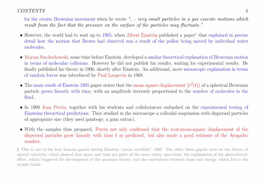
CONTENTS 6for the erratic Brownian movement when he wrote ". . . very small particles in a gas execute motions whichresult from the fact that the pressure on the surface of the particles may fluctuate."

• However, the world had to wait up to 1905, when Albert Einstein published a paper1 that explained in precisedetail how the motion that Brown had observed was a result of the pollen being moved by individual watermolecules.

• Marian Smoluchowski, some time before Einstein, developed a similar theoretical explanation of Brownian motionin terms of molecular collisions. However he did not publish his results, waiting for experimental results. Hefinally published his theory in 1906, shortly after Einstein. An additional, more mesoscopic explanation in termsof random forces was introduced by Paul Langevin in 1908.

• The main result of Einstein 1905 paper states that the mean square displacement 〈r2(t)〉 of a spherical Brownianparticle grows linearly with time, with an amplitude inversely proportional to the number of molecules in thefluid.

• In 1908 Jean Perrin, together with his students and collaborators embarked on the experimental testing ofEinsteins theoretical predictions. They studied in the microscope a colloidal suspension with dispersed particlesof appropriate size (they used gamboge, a gum extrac).

• With the samples thus prepared, Perrin not only confirmed that the root-mean-square displacement of thedispersed particles grow linearly with time t as predicted, but also made a good estimate of the Avogadronumber.

† This is one of the four famous papers during Einstein "annus mirabilis", 1905. The other three papers were on the theory ofspecial relativity, which showed that space and time are parts of the same entity, spacetime, the explanation of the photoelectriceffect, which triggered the development of the quantum theory, and the equivalence between mass and energy, which led to theatomic bomb.

CONTENTS 7

• Einstein’s explanation of Brownian motion, together with the outstanding experimental verification of Perrin’sexperiments, served as convincing evidence that atoms and molecules exist. Perrin was awarded the Nobel Prizein Physics in 1926 "for his work on the discontinuous structure of matter".

• It is an irony of fate that, just when atomic doctrine was on the verge of intellectual victory, Ludwig Boltzmannfelt defeated and committed suicide in 1906.

• Brownian motion plays an important role not only in a wide variety of systems studied within the traditionaldisciplinary boundaries of physical sciences but also in systems that are subjects of investigation in earth andenvironmental sciences, life sciences as well as in engineering and technology.

• However the greatest importance of Einstein’s theory of Brownian motion lies in the fact that experimentalverification of his theory silenced all skeptics who did not believe in the existence of atoms.

• Mathematically, Brownian motion is among the simplest of the continuous-time stochastic (or probabilistic)processes, and it is a limit of both simpler and more complicated stochastic processes (e.g. the random walk).This universality is closely related to the universality of the normal distribution (central limit theorem).

CONTENTS 8

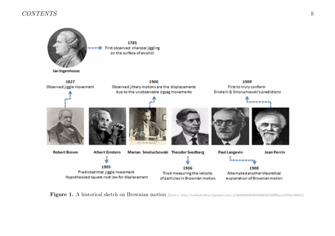
Figure 1. A historical sketch on Brownian motion [Source: http://radhakrishna.typepad.com/.a/6a00d83453b94569e20162ff35a1d1970d-600wi]

CONTENTS 9

Figure 2. Sketch of Brownian motion. Left panel: random trajectory of a mesoscopic particle immersed in amolecular fluid. The many random collisions of the fluid’s microscopic particles with the mesoscopic object (middelpanel) induce in the latter an erratic, intermitent motion in the latter. Right panel: Coarse-grained description ofthe mesoscopic particle position at time intervals τ .

2. Einstein theory

• A. Einstein in 1905 successfully introduced the first mathematical treatment of the erratic movement of theBrownian particles. Rather than focusing on the (complicated) trajectory of a single particle, Einstein introduceda probabilistic description valid for an ensemble of Brownian particles.

• First, Einstein introduced the concept of a coarse-grained description defined by a time τ such that differentparts of the trajectory separated by a time τ or larger can be considered independent. No attempt is made tocharacterize the dynamics at a timescale smaller than this coarse-grain time τ . Instead, we consider snapshotsof the system taken at time intervals τ (see right panel of Fig. 3).

• The second concept, probabilistic in nature, introduced by Einstein is that of the probability density function (orpdf) f (∆), for the three-dimensional distance ∆ = (∆x,∆y,∆z) traveled by the Brownian particle in a fixedtime interval τ .

CONTENTS 10• The only assumption one needs to make about the function f (∆) (besides the general condition of nonnegativityand normalization) comes from the fact that the collisions of the fluid molecules and the Brownian particle occurwith the same probability in any direction1. The absence of preferred directions translates to a symmetrycondition for f (∆), as

f (−∆) = f (∆) , ∀∆ ∈ R3 . (1)

• The third step in this description is to consider an ensemble of N Brownian particles in a large enough system.Also, we focus on large spatial scales, much larger than the size of a Brownian particle, so that we can definea density of the particles n(x, t) such that n(x, t) dx is the number of particles in the interval (x,x + dx) attime t.

• From the assumption that the parts of the trajectories separated a time interval τ are statistically independentand the conservation of particle number, it follows that the number of particles at location x at time t + τ willbe given by the number of particles at location x−∆ at time t multiplied by the probability that the particlejumps from x −∆ to x in an elementary time step τ , which is f (∆), and integrated for all the possible ∆values, i.e.

n(x, t + τ ) =∫R3 n(x−∆, t) f (∆)d∆ . (2)

This is the basic evolution equation for the number density n(x, t). From the technical point of view, it is acontinuity equation expressing particle conservation, i.e. that Brownian particles can neither be created, nor canthey disappear as a result of the collisions with the fluid molecules.

† We also disregard the effect of gravity in the Brownian particle, which would lead to a preferred direction in the movement.

CONTENTS 11• By Taylor expansion of the above expression

n(x, t + τ ) ≈ n(x, t) + τ∂n(x, t)∂t

, (3)

n(x−∆, t) ≈ n(x, t)−∆ ·∇n(x, t) + ∆2

2∇2n(x, t) . (4)

Therefore∫R3 n(x−∆, t) f (∆)d∆ ≈ n(x, t)

∫R3 f (∆)d∆−∇n(x, t) ·

∫R3 ∆ f (∆)d∆+ 1

2∇2n(x, t)

∫R3 ∆

2 f (∆)d∆ ,

(5)and making use of the normalization of the pdf f (∆) and the symmetry relation f (−∆) = f (∆), we simplifythe first term in the right-hand side of this equation and get rid of the second one. Hence we finally obtain thediffusion equation for the particle density field as

∂n(x, t)∂t

= D∇2n(x, t) , (6)

where the diffusion coefficient D is given in terms of the pdf f (∆) as

D = 12τ

∫R3 ∆

2 f (∆)d∆ = 〈∆2〉

2τ. (7)

• To solve this partial differential equation, we first need an initial condition. If initially all Brownian particlesare located at the origin, we thus have n(x, 0) = Nδ(x). The diffusion equation can be solved via differentmethods. One of the most common is via Fourier transform of the particle density field. In particular, we define

n(k, t) =∫R3 e

ik·xn(x, t) dx , (8)

CONTENTS 12and derive it with respect to time to obtain (after integrating by parts twice and neglecting boundary terms at∞)

∂n(k, t)∂t

= −Dk2n(k, t) ⇒ n(k, t) = Ne−Dk2t , (9)

where we have already used the initial condition mentioned above. Notice that n(k, t) is a Gaussian curve, soits inverse Fourier transform is also a Gaussian, namely

n(x, t) = N

(4πDt)3/2e−x2/4Dt . (10)

• Another, very instructive way of solving the diffusion equation is via dimensional analysis. For that, first notethat the n(x, t) is a particle density field so it has units of inverse volume, [n(x, t)] = L−d in dimension d, withL the unit of length. Moreover, the diffusion constant D defined above has units [D] = L2/T , with T the unitof time, and obviously [t] = T . The only nontrivial quantity that can be defined with units of length in theproblem is

√Dt, so (Dt)d/2n(x, t) is a dimensionless quantity which should depend only on other dimensionless

quantities. From variables x, t, D we can form a single dimensionless quantity x/√Dt. Therefore the most

general dependence of the density field on the basic variables that is allowed by dimensional analysis is

n(x, t) = 1(Dt)d/2

ρ(ζ) , ζ = x√Dt

. (11)

• The density depends on a single scaling variable rather than on two basic variables x and t. This remarkablefeature greatly simplifies analysis of the typical partial differential equations that describe nonequilibrium systems.Equation (11) is often referred to as the scaling ansatz. Finding the right scaling ansatz for a physical problemoften represents a large step toward a solution. For the diffusion equation, substituting in the ansatz (11) reducesthis partial differential equation to

2∇2ρ(ζ) + ζ ·∇ρ(ζ) + dρ(ζ) = 0 . (12)

CONTENTS 13

Figure 3. Time evolution of the density field for an initially localized ensemble of Brownian particles. It is a Gaussiancurve whose variance grows linearly with time, see Eq. (10). [Wikipedia. Source author: Bernard H. Lavenda]

Invoking both the normalization condition and the symmetry of ρ(ζ) around ζ = 0, so that ρ(ζ) = ρ(ζ), andintegrating twice the above equation, we obtain ρ(ζ) = (4π)−d/2e−ζ2/4 for arbitrary dimension d, and using thatζ = x/

√Dt we recover the Gaussian solution for n(x, t) described above.

• Whatever the solution method, from the Gaussian solution n(x, t) it follows that the average position of theBrownian particle is 〈x(t)〉 = 0 and that the average square position increases linearly with time, namely〈x(t)2〉 = 6Dt in d = 3 dimensions. As mentioned above, this prediction was successfully confirmed in Perrin’sexperiments and contributed decisively to the acceptance of the atomic/molecular theory of matter.

CONTENTS 143. Langevin theory, Stokes-Einstein relation and Green-Kubo formula

• However successful Einstein’s approach was, it is very phenomenologicaland cannot yield, for instance, an explicit expression for the diffusioncoefficient in terms of microscopic quantities.

• Paul Langevin (1908) initiated a different approach which, in some ways,can be considered complementary to the previous one. In his approach,Langevin focused on the trajectory of a single Brownian particle andwrote down Newton’s equation Force = mass × acceleration.

• The trajectory of the Brownian particle is highly erratic and therefore itsdescription would demand a peculiar kind of force. Langevin consideredtwo types of forces acting on the Brownian particle: the usual frictionforces which, according to Stokes law, would be proportional to thevelocity, and a sort of "fluctuating" force ξ(t), which represents the"erratic" force that comes from the action of the fluid molecules on theBrownian particle.

• The equation of motion for the Brownian particle becomes then

mdv

dt= −6πηav + ξ , (13)

where η is the viscosity coefficient and a is the radius of the Brownian particle (which is assumed to be spherical).Multiplying both sides of by x, and noting that v = dx

dt , one gets

m

2d2x2

dt2−m

dxdt

2= −3πηadx

2

dt+ x · ξ . (14)

CONTENTS 15• Langevin made two assumptions about the fluctuating force ξ(t): that it has mean 0 (collisions do not push theBrownian particle in any preferred direction) and that it is uncorrelated to the actual position of the Brownianparticle (the action of the molecules of fluid on the Brownian particle is the same no matter the location of theBrownian particle), that is

〈ξ(t)〉 = 0 ; 〈x · ξ(t)〉 = 〈x〉 · 〈ξ(t)〉 = 0 . (15)

• Taking the averages with respect to all realizations of the random force ξ(t) in the above differential equationand using the previous conditions on the statistics of ξ(t), one gets

m

2d2〈x2〉dt2

= m〈v2〉 − 3πηad〈x2〉

dt, (16)

which is an equation for the average square position of the Brownian particle.

• Langevin assumed that we are now in a regime in which thermal equilibrium between the Brownian particle andthe surrounding fluid has been reached. In particular, this implies that, according to the equipartition theorem,the average kinetic energy of the Brownian particle is 〈mv2/2〉 = 3kT/2 (k is Boltzmann’s constant and T isthe fluid temperature).

• One can now solve the previous equation and find that, after some transient time, the asymptotic mean squaredisplacement is given

〈x2(t)〉 = kT

πηat . (17)

This is nothing but Einstein’s diffusion law, 〈x(t)2〉 = 6Dt, but now we have an explicit expression for thediffusion coefficient in terms of other macroscopic variables

D = kT

6πηa= RT

6πηaNAv, (18)

CONTENTS 16where we have used in the last equality the definition of Boltzmann’s constant k in terms of the ideal gas constantR and Avogadro’s number NAv, i.e. k = R/NAv. This last equation is known as Stokes-Einstein relation.

• In this way, by measuring the Brownian particle diffusion coefficient and the fluid’s viscosity (two macroscopicobservables) we can obtain an indirect measurement of the size a of the fluid’s molecules or equivalently ofAvogadro’s number!

3.1. A simple example of Green-Kubo formula for transport coefficients

• In this section we will derive a simple relation between the diffusion constant and the integral of the equilibriumtime-correlation function of the velocity of a Brownian particle. This is a particular (and very illustrative)example of the Green-Kubo formulae relating transport coefficients and equilibrium time-correlation functions,a main result of nonequilibrium statistical mechanics.

• Let’s consider the net displacement of the Brownian particle’s position during the interval from 0 to t. This canbe written as

x(t) =∫ t0 dsv(s) , (19)

where v(s) is the velocity of the particle at time s.

• The ensemble average of the mean squared displacement is

〈x(t)2〉 =⟨ ∫ t

0 ds1∫ t0 ds2 v(s1) · v(s2)

⟩=

∫ t0 ds1

∫ t0 ds2 〈v(s1) · v(s2)〉 (20)

Note that the integral contains the time-correlation function of the velocity at times s1 and s2.

• We now take the time derivative and combine two equivalent terms on the right-hand side,d

dt〈x(t)2〉 = 2

∫ t0 ds 〈v(t) · v(s)〉 (21)

CONTENTS 17• The velocity correlation function is an equilibrium average and cannot depend on any arbitrary origin of thetime axis. It can depend only on the time difference t− s = u, so that

d

dt〈x(t)2〉 = 2

∫ t0 ds 〈v(t− s) · v(0)〉 = 2

∫ t0 du 〈v(u) · v(0)〉 (22)

• The velocity correlation function generally decays to zero in a short time; in simple liquids, this may be of theorder of picoseconds. On the other hand, the diffusion equation is expected to be valid only at times much longerthan a molecular time.

• In the limit of large tt, according to Einstein’s theory 〈x(t)2〉 = 6Dt, so the left-hand side of the above equationapproaches 6D. In the same regime, the right-hand side approaches a time integral from zero to infinity.

• Therefore we have derived the simplest example of the Green-Kubo relation of a transport coefficient to a timecorrelation function,

D = 13∫ ∞0 du 〈v(u) · v(0)〉 (23)

CONTENTS 184. Stochastic differential equations and Fokker-Planck equations

• Langevin’s equation is an example of stochastic differential equation, and Langevin’s random force ξ(t) is anillustration of a stochastic process. The natural language to understand both concepts is that of probabilitytheory.

4.1. Stochastic differential equations

• A stochastic differential equation is a differential equation that contains a stochastic process η̂(t): that is, anequation of the form

dx̂(t)dt

= G(x̂(t), t, η̂(t)

)(24)

where G is a given function that depends, in general, on the variable x(t), on the time t, and on the stochasticprocess η̂(t).

• A stochastic process is a family x̂(t) of random variables depending on some continuous, real parameter t.In most applications, t is a physical time and the stochastic process can be thought as performing multipleprobabilistic experiments one at each time instant.

• Stochastic processes (as well as random variables) are usually denoted in the mathematical literature with a"hat"-symbol, x̂(t), to distinguish them from a particular realization of the stochastic process, i.e. from aparticular realization or trajectory of the set of probabilistic experiments which give rise to a stochastic process.The stochastic process can be seen as the collection of all these possible trajectories.

• A stochastic differential equation can be seen as a family of ordinary differential equations, one for each outcomeof all the successive probabilistic experiments associated with the stochastic process η̂(t). As a consequence, forany given initial condition x0 at time t0, one has a family of possible trajectories.

CONTENTS 19• Therefore, x̂(t), which is the collection of all these possible trajectories, has to be viewed also as a stochasticprocess and this is why we label it with the "hat" symbol. However, x̂(t) is not an arbitrary stochastic process,rather it depends on η̂(t) in a specific manner determined by the stochastic differential equation, and, as aconsequence, the statistical properties of x̂(t) depend on the statistical properties of η̂(t).

• Strictly speaking, "solving the stochastic differential equation" means to provide the complete characterizationof the stochastic process x̂(t), namely to give all the m-times probability density functions (pdfs)f (x1, . . . , xm; t1, . . . , tm), in terms of the statistical properties of η̂(t). However, one has to understand thata complete characterization of a general stochastic process implies the knowledge of a function of an arbitrarynumber of parameters and is very difficult to carry out in practice.

• On many occasions, one is happy if one can give just the one-time pdf f (x; t) and the two-times pdff (x1, x2; t1, t2). In terms of those, it is possible to compute the trajectory averages

〈x̂(t)n〉 =∫ ∞−∞

dx xnf (x; t) (25)

and the time correlations〈x̂(t1)nx̂(t2)m〉 =

∫ ∞−∞

dx xn1xm2 f (x1, x2; t1, t2) . (26)

• In general, the function G can depend on the stochastic process η̂(t) in an arbitrary way. However, many systemsof interest can be described by stochastic differential equations in which η̂(t) appears linearly, namely

dx̂(t)dt

= q (x̂(t)) + g (x̂(t)) η̂(t) . (27)

This kind of stochastic differential equations are called Langevin equations in honor of one of the first scientiststo use them to describe a physical phenomenon.

CONTENTS 20• In this case (Langevin equations), the independent stochastic process η̂(t) is usually referred to as noise, anotation that comes from the early days of radio broadcasting when the random fluctuations in the electricalsignals taking place in the emitter during the propagation in the atmosphere or at the receiver device led tonoises that were actually heard on top of the radio emission.

• Terminology: Following this notation, the term g (x̂(t)) η̂(t) in Eq. (27) is referred to as the noise term ordiffusion term whereas q (x̂(t)) is the deterministic term or drift term. One distinguishes the case in which thefunction g (x̂(t)) is a constant, in which case the noise is said to be additive. Otherwise, the noise is said to bemultiplicative.

• For the sake of simplicity in the notation, from now on we will drop the "hats" from the stochastic process andtherefore we write the Langevin differential equation as

dx(t)dt

= q (x(t)) + g (x(t)) η(t) . (28)

4.2. Fokker-Planck equations

• So far, we have focused on trajectories to describe stochastic processes following the initial Langevin approachfor Brownian motion.

• An alternative approach introduced by Einstein focuses on probabilities rather than in trajectories and, as ithappens with the Langevin approach, it can be extended way beyond the Brownian motion.

• In what follows, we are going to determine an equation for one-time probability distribution for a stochasticprocess described by a Langevin equation with Gaussian white noise. This is called the Fokker-Planck equationand it is a generalization of the diffusion equation obtained by Einstein to describe the Brownian process.

CONTENTS 21• To be more precise, we want to find an equation for the one-time probability distribution function f (x, t) fora stochastic process x(t) which arises as a solution of a stochastic differential equation with a Gaussian whitenoise ξ(t), defined such that 〈ξ(t)〉 = 0 and 〈ξ(t)ξ(t′)〉 = δ(t− t′), i.e.

dx(t)dt

= q(x(t)) + g(x(t))ξ(t) . (29)

• To obtain this equation, we have to average over all possible initial conditions and all realizations of the stochasticprocess ξ(t). The derivation, which lies outside the scope of the present discussion (see however the appendix),leads to the so-called Fokker-Planck equation for the probability density function:

∂f (x; t)∂t

= − ∂

∂x[q(x)f (x; t)] + 1

2∂

∂x

g(x) ∂∂x

[g(x)f (x; t)] . (30)

• This framework can be extended to the case of Langevin equations for multidimensional variables, and even tofield-theoretic Langevin equations which emerge in the description of equilibrium and nonequilibrium criticalphenomena, nonequilibrium dynamics, transport problems, etc.

CONTENTS 225. The random walk model

• Arguably, the most well-known example of a stochastic process is that of the random walk. Moreover, thecontinuum (large scale) limit of a (3-dimensional) random walk offers a good description of Brownian motion. Italso serves as a simple model to understand the physics of polymers, motion in cells, financial markets, etc.

• Here for simplicity we will focus on the one-dimensional random walk, though all results can be easily generalizedto arbitrary dimensions.

• The probabilistic experiment is now a series of binary results representing, for instance, the outcome of repeatedlytossing a coin:

χ ≡ (−1,−1,+1,+1,−1,+1,−1,−1,+1,+1,−1,−, 1, . . .) = {χk, k = 1, 2, . . .} (31)

where +1 means "heads" and −1 means "tails" .

• Consider that the tossing takes place at given times 0, τ, 2τ, . . . To the outcome of this set of probabilisticexperiments, we associate a one-dimensional function x(t) which starts at x(0) = 0 and that moves to the right(left) at time kτ an amount +a (−a) if the k-th result of the tossed coin was +1 (−1).

• In the intermediate times between two consecutive tossings, namely in the times between k and (k + 1), thesystem just remains in the same location. Fig. 4 shows a typical trajectory.

• The random walk constitutes an example of a Markov process, as the probability of having a particular value ofthe position at time (k + 1)τ depends only on the particle’s location at time kτ and not on the way it got tothis location.

CONTENTS 23

Figure 4. Example of a random walk trajectory. We have taken τ = a = 1 and plotted the resulting trajectory aftera large number of steps (105). In the inset, we see the fine detail with the discrete jumps occurring at times whichare multiples of τ .

• Starting at x = 0 at time t = 0, the location of the random walker after tossing the coin n times is given bythe number of steps n+ increasing x (number of "heads") minus the number of steps decreasing x, n− = n− n+(number of "tails"),

x(nτ ) = (n+ − n−)a = (2n+ − n)a . (32)

• The probability of having n+ "heads" after n throws is given by a binomial distribution with probability p = 1/2

P (n+) = nn+

2−n = n!n+!(n− n+)!

2−n . (33)

CONTENTS 24In general, a binomial distribution with probability p has the form

fN̂B(n+) =

nn+

pn+(1− p)n−n+ . (34)

We denote as N̂B(p, n) a random variable obeying a binomial distribution with probability p and number ofrepetitions n. Its mean value and variance are given by

〈N̂B〉 = np , (35)σ2[N̂B] = 〈N̂2

B〉 − 〈N̂B〉2 = np(1− p) . (36)

• In this way, the probability that the walker is at a location x = ra after a time t = nτ is

P (x(nτ ) = ra) = nn+r

2

2−n . (37)

• Using now the binomial distribution properties, in particular the first two central moments, we find that

〈x(nτ )〉 = (2〈n+〉 − n)a = 0 , (38)

〈x(nτ )2〉 = (4〈n2+〉 − 4〈n+〉n + n2)a2 = na2 = nτ

a2

τ, (39)

where we have used that 〈n+〉 = n2 and 〈n2

+〉 = n(n+1)4 . The last expression is strongly reminiscent of the mean

squared displacement formula for Brownian motion.

• It can be easily probed that in the limit n� 1 the binomial distribution can be well approximated by a Gaussiandistribution (of mean np and variance np(1− p) for a N̂B(p, n) variable).

CONTENTS 25• If we now take the continuum limit n→∞, τ → 0, r →∞, a→ 0 while preserving a finite value for t = nτ ,x = ra, and D = a2/τ , it can be shown that the random walk process converges to the so-called Wiener processW (t), characterized by a Gaussian probability distribution function with zero mean and variance Dt, namely

f (x; t) = 1√2πDt

exp− x2

2Dt

. (40)

• This is exactly the solution of the diffusion equation in Einstein’s theory of Brownian motion in one dimension.

5.1. A glimpse at rare events and large deviations

• The previous discussion referred to the probability distribution for finding the random walker at some positionat a given time, f (x; t).

• We now turn our attention to the sample average position of the random walker. Consider the following average

Sn(χ) = 1n

n∑k=1

χk = 1n

(n+ − n−) = 1n

(2n+ − n) (41)

In this way, for a given trajectory χ, the time-averaged position of the random walker is x̄n(χ) = Sn(χ)a.

• What is the probability of observing a sample average position sa after n steps? This is nothing but theprobability that Sn(χ) = s, or equivalently the probability of obtaining n+ = n(1 + s)/2 "heads" after n throws,i.e.

P (Sn = s) = nn2 (1 + s)

2−n (42)

• ntuitively, the sample average position of the random walker should converge for large enough n to the actualaverage position of the random walker, which is just 0.

CONTENTS 26• For large n, we may use now Stirling approximation n! ≈ nne−n so

P (Sn = s) ≈ nne−n

[n2 (1 + s)]n2 (1+s)e−n

2 (1+s) [n2 (1− s)]n2 (1−s)e−n

2 (1−s)2−n =[(1 + s)

12(1+s) (1− s)

12(1−s)

]−n. (43)

• In this way, the probability that the sample average position Sn of a random walker takes a given value obeys alarge deviation principle for large n

P (Sn = s) ≈ e−nI(s) , (44)with I(s) a large deviation function of the form

I(s) = 12

[(1 + s) ln(1 + s) + (1− s) ln(1− s)] . (45)

• The large deviation function measures the rate at which the sample mean Sn concentrates around the averagevalue of the distribution (s = 0 in this case) as the sample size n grows.

• The above large deviation principle means that sample averages differing appreciable from the true average areexponentially unlikely with n, the sample size.

• The large deviation function quantifies the probability of both typical and rare events for a given stochasticprocess.

• Large deviation functions (LDFs) as the one here introduced play a crucial role in equilibrium and nonequilibriumstatistical physics. In equilibrium systems, the thermodynamic potentials associated to the different ensembles(canonical, micro- and macro-canonical, etc.) can be seen as large deviation functions associated to the differentconserved observables. In nonequilibrium systems LDFs play the role of thermodynamic-like potentials, eventhough we do not have yet a suitable macroscopic theory for systems out of equilibrium.

CONTENTS 27

CONTENTS 286. Appendix: Derivation of Fokker-Planck equation

• So far, we have focused on trajectories to describe stochastic processes following the initial Langevin approachfor Brownian motion.

• The alternative approach introduced by Einstein focuses on probabilities rather than in trajectories and, as ithappens with the Langevin approach, it can be extended way beyond the Brownian motion.

• In what follows, we are going to determine an equation for one-time probability distribution for a stochasticprocess described by a Langevin equation with white noise. This is called the Fokker-Planck equation and it isa generalization of the diffusion equation obtained by Einstein to describe the Brownian process.

• To be more precise, we want to find an equation for the one-time probability distribution function f (x, t) fora stochastic process x(t) which arises as a solution of a stochastic differential equation with a Gaussian whitenoise ξ(t), defined such that 〈ξ(t)〉 = 0 and 〈ξ(t)ξ(t′)〉 = δ(t− t′), i.e.

dx(t)dt

= q(x(t)) + g(x(t))ξ(t) . (46)

This is to be understood in the Stratonovich interpretation.

6.1. Deterministic dynamics and sampling over initial conditions

• Let us consider first the corresponding deterministic equationdx(t)dt

= q(x(t)) , x(t = 0) = x0 . (47)

The solution of this equation is a (deterministic) function x(t) = F (t, x0). Nevertheless, for our purposes, we cansee x(t) as a random variable whose probability density function ρ(x; t) gives the probability to find the system

CONTENTS 29at a given location x in phase space at a time t. As the trajectory followed by the system is uniquely determinedonce the initial condition is given, this probability is zero everywhere except at the location x = F (t, x0).Therefore, the probability density function is a delta function, given by

ρ(x; t) = δ(x− F (t, x0)) . (48)

• We can now transform x(t) into a stochastic process by simply letting the initial condition x0 to become a randomvariable. We have now an ensemble of trajectories, each one starting from a different initial condition x0. In thiscase, the probability density function ρ(x, t) is obtained by averaging the above pdf over the distribution of theinitial conditions

ρ(x; t) = 〈δ(x− F (t, x0))〉x0 . (49)In fact, ρ(x, t) can be seen as a density function.

• To visualize it, we assume that at time t = 0 we have unleashed a large number of particles N with one particleat each of the initial conditions we are considering in our ensemble. We let the particles evolve according to thedynamics and, after a time t, ρ(x, t)dx measures the fraction of particles located in the interval (x, x + dx)

ρ(x, t)dx = # particles in (x, x + dx) at time ttotal # of particles

= n(x, t)N

dx . (50)

• Assuming there are no sinks nor sources of particles, then the number of particles at a given location changes asa result of the number of particles crossing the borders. Let J(x, t) be the flux of particles:

J(x, t)dx = # particles that cross the point x in the interval (t, t + dt)N

. (51)

J has a direction. For convenience, we consider J > 0 if the particle moves to the right. Then

ρ(x; t + dt)dx− ρ(x; t)dx = J(x, t)dt− J(x + dx, t)dt . (52)

CONTENTS 30• The first term on the left-hand side (LHS) is the final number of particles at x, whereas the second is the initialone. Thus, the LHS corresponds to the variation of the number of particles at x from time t to time t+ dt. Onthe right-hand side (RHS), the first term is the number of particles that have entered or left during the interval(t, t + dt) through the left boundary, whereas the second term measures the number of particles that crossedthe right boundary.

• Therefore, one hasρ(x; t + dt)− ρ(x; t)

dt= J(x, t)− J(x + dx, t)

dx(53)

which in the continuous limit corresponds to

∂ρ(x; t)∂t

= −∂J(x, t)∂x

(54)

which is nothing but the continuity equation.

• As particles move following a deterministic dynamics given by dx(t)dt = q(x(t)), trajectories cannot cross and

therefore in a one-dimensional system they cannot advance from one to the other. The particles that will crossthe point x in the interval (t, t + dt) are all those located in the interval dx = q(x)dt. Therefore,

J(x, t) = n(x, t)N

dx

dt= ρ(x; t)q(x) . (55)

Replacing this in the above continuity equation, one gets the Liouville equation

∂ρ(x; t)∂t

= − ∂

∂x[q(x)ρ(x; t)] . (56)

CONTENTS 316.2. Full stochastic dynamics

• We consider now the full stochastic differential equation

dx(t)dt

= q(x(t)) + g(x(t))ξ(t) . (57)

• We can repeat the above argument for a given realization of the noise term. The probability density functionf (x; t) will be the average of ρ(x; t) with respect to the noise distribution:

f (x; t) = 〈ρ(x; t)〉ξ = 〈δ(x− x(t, x0))〉x0,ξ . (58)

• ρ(x; t) satisfies the continuity equation. Now the current is given by

J(x, t) = ρ(x; t)dx(t)dt

= ρ(x; t) [q(x(t)) + g(x(t))ξ(t)] . (59)

Therefore∂ρ(x; t)∂t

= − ∂

∂x[(q(x) + g(x(t))ξ(t))ρ(x; t)] . (60)

• Taking now the average over the noise term, we get

∂f (x; t)∂t

=⟨∂ρ(x; t)

∂t

⟩ξ

= − ∂

∂x

⟨[q(x) + g(x(t))ξ(t)] ρ(x; t)

⟩ξ

= − ∂

∂x

[q(x)

⟨ρ(x; t)

⟩ξ

]− ∂

∂x

[g(x(t))

⟨ξ(t)ρ(x; t)

⟩ξ

]. (61)

The averages on the first term of the right-hand side (RHS) can be easily performed, 〈ρ(x; t)〉 = f (x; t).

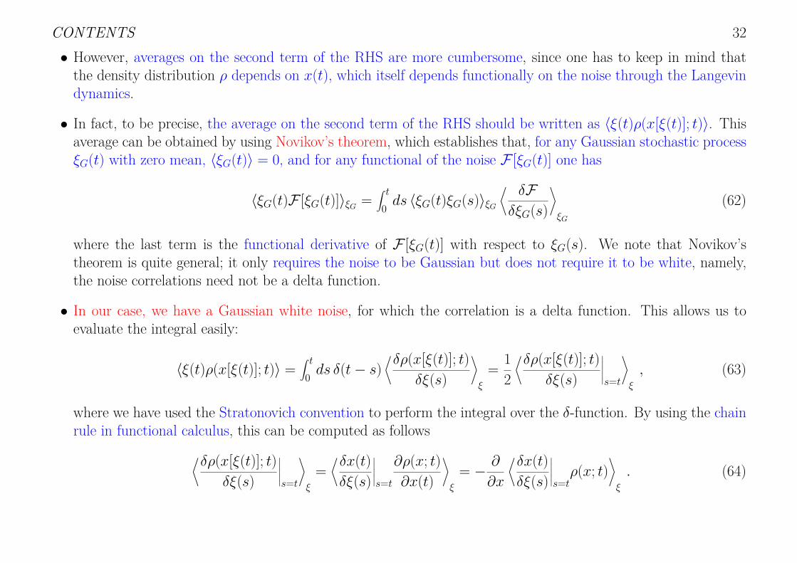
CONTENTS 32• However, averages on the second term of the RHS are more cumbersome, since one has to keep in mind thatthe density distribution ρ depends on x(t), which itself depends functionally on the noise through the Langevindynamics.

• In fact, to be precise, the average on the second term of the RHS should be written as 〈ξ(t)ρ(x[ξ(t)]; t)〉. Thisaverage can be obtained by using Novikov’s theorem, which establishes that, for any Gaussian stochastic processξG(t) with zero mean, 〈ξG(t)〉 = 0, and for any functional of the noise F [ξG(t)] one has

〈ξG(t)F [ξG(t)]〉ξG=

∫ t0 ds 〈ξG(t)ξG(s)〉ξG

⟨ δFδξG(s)

⟩ξG

(62)

where the last term is the functional derivative of F [ξG(t)] with respect to ξG(s). We note that Novikov’stheorem is quite general; it only requires the noise to be Gaussian but does not require it to be white, namely,the noise correlations need not be a delta function.

• In our case, we have a Gaussian white noise, for which the correlation is a delta function. This allows us toevaluate the integral easily:

〈ξ(t)ρ(x[ξ(t)]; t)〉 =∫ t0 ds δ(t− s)

⟨δρ(x[ξ(t)]; t)δξ(s)

⟩ξ

= 12

⟨δρ(x[ξ(t)]; t)δξ(s)

∣∣∣∣∣s=t

⟩ξ

, (63)

where we have used the Stratonovich convention to perform the integral over the δ-function. By using the chainrule in functional calculus, this can be computed as follows

⟨δρ(x[ξ(t)]; t)δξ(s)

∣∣∣∣∣s=t

⟩ξ

=⟨δx(t)δξ(s)

∣∣∣∣∣s=t

∂ρ(x; t)∂x(t)

⟩ξ

= − ∂

∂x

⟨δx(t)δξ(s)

∣∣∣∣∣s=tρ(x; t)

⟩ξ

. (64)

CONTENTS 33• To evaluate the functional derivative of the stochastic process x(t) with respect to the noise, we use a formalsolution of the Langevin stochastic differential equation, namely

x(t) = x0 +∫ t0 ds q(x(s)) +

∫ t0 ds g(x(s))ξ(s) . (65)

Thenδx(t)δξ(s)

∣∣∣∣∣s=t

= g(x(t)) (66)

and ⟨δρ(x[ξ(t)]; t)δξ(s)

∣∣∣∣∣s=t

⟩ξ

= − ∂

∂x

[g(x(t)) 〈ρ(x; t)〉ξ

]= − ∂

∂x[g(x(t))f (x; t)] . (67)

• Using this result in Eq. (61) above, we finally get the Fokker-Planck equation for the probability density function:

∂f (x; t)∂t

= − ∂

∂x[q(x)f (x; t)] + 1

2∂

∂x

g(x) ∂∂x

[g(x)f (x; t)] . (68)

• The procedure we have used to derive the Fokker-Planck equation for a single variable can be extended to thecase of several variables. Consider a set of stochastic variables x = (x1, x2, . . . , xN) whose dynamics is given bythe set of Langevin equations to be considered in the Stratonovich interpretation

dxidt

= qi(x, t) +N∑j=1

gij(x, t)ξj(t) i = 1, . . . , N (69)

where we allow for the drift terms qi(x, t) and diffusion terms gij(x, t) to explicitly depend on the time. ξj(t)are uncorrelated Gaussian white noises with zero mean, that is

〈ξi(t)〉 = 0 ; 〈ξi(t)ξj(s)〉 = δijδ(t− s) ∀i, j ∈ [1, N ] (70)

CONTENTS 34• By using a straightforward extension of the method used for one variable, one can prove that the one-timeprobability density function f (x; t) satisfies the following multivariate Fokker-Planck equation

∂f (x; t)∂t

= −N∑i=1

∂

∂xi[qi(x, t)f (x; t)] + 1

2N∑

i,j,k=1

∂

∂xi

gik(x, t) ∂

∂xj[gjk(x, t)f (x; t)]

. (71)

• It can also be written in the form of a continuity equation

∂f (x; t)∂t

+N∑i=1

∂

∂xiJi(x, t) = 0 , (72)

where the probability currents Ji(x, t) are given by

Ji(x, t) = qi(x, t)f (x; t)− 12

N∑j,k=1

gik(x, t) ∂

∂xj[gjk(x, t)f (x; t)]

. (73)

• If qi(x, t) and gij(x, t) do not depend explicitly on time, i.e. qi(x, t) = qi(x) and gij(x, t) = gij(x), then theFokker-Planck equation is called homogeneous.