Available online at www.sciencedirect.com

Physica A 335 (2004) 339–358www.elsevier.com/locate/physa

Brownian dynamics: divergence ofmobility tensor

E. Wajnryba, P. Szymczakb;∗, B. CichockibaInstitute of Fundamental Technological Research, Polish Academy of Sciences, �Swie�tokrzyska 21,

Warsaw, 00-049, PolandbInstitute of Theoretical Physics, Warsaw University, Hoza 69, Warsaw, 00-618, Poland

Received 16 October 2003

Abstract

The mobility tensor for many spheres suspended in a viscous 3uid is considered. An ana-lytical formula for the divergence of this tensor is derived. It is then applied in calculationsof long-time collective di6usion coe7cient of hard-sphere suspension by means of Browniandynamics method.c© 2003 Elsevier B.V. All rights reserved.

PACS: 83.10.Mj; 82.70.Dd; 66.10.Cb; 47.15.Gf

Keywords: Brownian dynamics; Hydrodynamic interactions; Di6usion coe7cient

1. Introduction

The Brownian dynamics method is a powerful numerical tool for exploring the evo-lution and properties of interacting Brownian particle systems. In the simplest case,such a system consists of N identical spherical particles performing Brownian motionin an incompressible viscous 3uid at temperature T . On the time-scale characteristicfor light scattering experiments the evolution of the con@guration space distributionfunction P(X ; t) is described by the generalized Smoluchowski equation [1]

99t P(X ; t) =

N∑i; j=1

∇j · �ttji(X) · [kBT∇i + Fi]P(X ; t) ; (1.1)

∗ Corresponding author.E-mail address: piotrek@fuw.edu.pl (P. Szymczak).

0378-4371/$ - see front matter c© 2003 Elsevier B.V. All rights reserved.doi:10.1016/j.physa.2003.12.012

340 E. Wajnryb et al. / Physica A 335 (2004) 339–358

where X =(R1;R2 : : : ;RN ), with Ri being the position of ith particle and Fi the forceacting on it. Next, ∇i denotes the gradient with respect to the position of particlei and �tt is the translational mobility matrix. The latter is obtained by solving thehydrodynamic problem of @nding the velocities of the particles, Ui ; i = 1; : : : ; N , interms of the forces acting on them (in the absence of torques)

Ui =∑j

�ttijFj : (1.2)

In general, due to hydrodynamic interactions, the mobility matrix depends on con@gu-ration X and is nondiagonal in particle indices.The numerical algorithm to calculate the mobility matrix using multipole expansion

method is well established [2–7] and has been tested extensively in a number of studies.This algorithm has been extended in the present work to incorporate a scheme ofcalculating divergence of mobility matrix. Although in principle this can be done bynumerical di6erentiation of �tt , such a scheme is not only numerically expensive butalso inaccurate. Instead, we calculate the divergence of mobility matrix analyticallywith use of the multipole expansion method.Divergence of mobility matrix is an important object for studying the dynamics

of interacting Brownian particles. In particular, it is needed in Brownian dynamicssimulations of a system governed by the Smoluchowski equation. It can be shown [8]that a @xed time-step (coarse) realization of the stochastic process described by theSmoluchowski equation is constructed by advancing the particles according to

Ri(t +It) = Ri(t) + kBT∑j

∇j · �ttji(t)It +∑j

�ttij(t) · Fj(t)It + �i(It) :

(1.3)

The vector �i(It) is a random displacement with Gaussian distribution of zero meanand covariance given by

〈�i(It)�j(It)〉 = 2kBT�ttij(t)It : (1.4)

As can be seen from the above, key quantities needed to compute the trajectories arethe mobility matrix and its divergence summed over all particles

di =∑j

∇j · �ttji : (1.5)

As the mobility matrix depends in a nontrivial way on positions of all particles inthe system, its computation is highly time and memory consuming. Thus various ap-proximations are usually resorted to in order to reduce the complexity. The crudestapproximation is to write �tt as the sum of terms describing two-body interactionsgiven by Oseen or Rotne–Prager tensors [8–15]. However, in any two-body approxima-tion the vector di vanishes. Even if more sophisticated schemes of calculating mobilitymatrix are used in Brownian dynamics simulations, the divergence term is often eitherneglected or calculated by a ‘brute-force’ numerical di6erentiation. The latter is bothinaccurate and extremely slow since one needs to calculate �tt at least 3N times toobtain di for a given con@guration.

E. Wajnryb et al. / Physica A 335 (2004) 339–358 341

Another problem in which the divergence of mobility matrix plays a central role iscalculation of long-time collective di6usion coe7cient, Dl

c. This coe7cient is de@nedin terms of intermediate scattering function F(k; t) by

Dlc = lim

k→0

1k2

limt→∞

d logFdt

: (1.6)

In the system of interacting Brownian particles there is a nonzero di6erence betweenthe value of the long-time di6usion coe7cient and that of the short-time one given by

Dsc = lim

k→0

1k2

limt→0

d logFdt

: (1.7)

This di6erence is due to the memory e6ects in the system which are associated withthe relaxation of the particle distribution function [16]. The strength of these e6ects ismeasured by a dimensionless factor � [17]

�=Ds

c − Dlc

Dsc

: (1.8)

The explicit expression for this factor reads

�= limk→0

∫ ∞

t=0M (k; t) ; (1.9)

where the memory function M (k; t) is closely related to the autocorrelation functionof the divergence of mobility tensor. For example, for hard-sphere suspensions M (k; t)reads [18,16]

M (k; t) =kBT 〈∑N

i; j=1 di(0) · dj(t) eik·(Rj(t)−Ri(0))〉〈∑N

i; j=1 Tr �ttij eik·Rji〉 ; (1.10)

where Tr stands for trace and angular brackets denote equilibrium average. Again, incrude approximations for �tt the vector di vanishes and the information about memorye6ects is lost as M (k; t)=0. Hence an accurate and e7cient algorithm of calculating di isessential for investigation of memory e6ects. E7ciency of the algorithm is particularlyimportant since the numerical complexity is usually a key issue when computing theproperties of interacting Brownian particle system.The outline of the paper is as follows. Section 2 reviews the numerical scheme for

calculating hydrodynamic interactions between spheres in Stokes 3ow. In particular, werecall the method of obtaining the mobility matrix using multipole expansion technique.Next, in Section 3, this formalism is applied to derive an expression for divergenceof mobility matrix. It turns out that it is possible to represent di in terms of the samefunctions as those that appear in multipole representation of mobility matrix. Finally, inSection 4 the memory factor � (1.8) is calculated numerically using Brownian dynamicssimulations. In the calculation the divergence of mobility tensor is used twice: in theexpression for memory function as well as in Brownian dynamics algorithm (1.3) itself.

2. Hydrodynamic interactions between many spheres: mobility problem

Consider N spheres of equal radii a, which undergo external forces F1; : : : ;FN andexternal torques T1; : : : ;TN (in the following abbreviated as F and T), and which

342 E. Wajnryb et al. / Physica A 335 (2004) 339–358

are immersed in an incompressible 3uid of viscosity �. Assume that the Reynoldsnumber is low and that the 3uid velocity and pressure, v(r) and p(r), satisfy thestationary Stokes equations [19]

�∇2v(r) − ∇p(r) = 0; ∇ · v= 0 ; (2.1)

with the stick boundary conditions at the particle surfaces Si:

v(r) = wi(r) ≡ Ui + �i × (r− Ri) for r∈ Si; i = 1; : : : ; N ; (2.2)

where U1; : : : ;UN and �1; : : : ;�N (in the following abbreviated as U and �) are thetranslational and the rotational velocities of all the particles.To solve Eqs. (2.1)–(2.2), the density fi(r) of induced forces [20–22] is introduced

for each particle i=1; : : : ; N . These forces, located at the particle surfaces, are exertedonto the 3uid by the spheres and are determined by the boundary conditions (2.2). Therigid body motion of the particles may be now interpreted as a @ctitious 3uid 3ow for|r−Ri|6 a, which obeys the Stokes equations (2.1). In this way Eqs. (2.1), with theadditional source term at the r.h.s., equal to −∑N

i=1 fi(r), may be extended onto thewhole space [20–22]. Their solution for an unbounded 3uid, which is at rest at in@nity,v(r), can be written as:

v(r) =N∑

j=1

∫T(r− r′) fj(r′) dr′ ; (2.3)

where T denotes the Oseen tensor [19]:

T(r) =1

8��r(I + rr) : (2.4)

Now let us choose a particle i and consider Eq. (2.3) at its surface Si. Taking intoaccount the boundary conditions (2.2), one can write Eq. (2.3) in terms of integraloperators as

wi = Z−10 (i) fi +

∑j �=i

G(ij) fj : (2.5)

In the above equation we decomposed the integral operator at the r.h.s. of Eq. (2.3)into two parts. The @rst part, given in terms of the one-particle friction operator Z0(i)[23], describes the contribution to the velocity of particle i from the induced forceslocated on the same particle (i)

[Z−10 (i)fi](r) ≡

∫T(r; r′) · fi(r′) dr′; r∈ Si : (2.6)

The second part involves Green operators [24,25] G(ij), where j=1; : : : ; N , but j = i,which account for the contributions to wi coming from the particles other than i

[G(ij)fj](r) ≡∫T(r; r′) · fj(r′) dr′; i = j; r∈ Si : (2.7)

To solve the integral equation (2.5), the multipole expansion is applied [4,5,7]. Theinduced forces as well as velocity @elds are then represented by in@nite set of multi-poles. The multipoles are labeled by three multipole indices l; m; �, where l=1; 2; : : : ;

E. Wajnryb et al. / Physica A 335 (2004) 339–358 343

while m= −l; : : : ;+l, and � = 0; 1; 2. The @rst two multipoles (l= 1; � = 0; 1) of theinduced force fi are: the total force Fi and the total torque Ti acting on spherei. On a level of velocity @eld the multipoles l = 1; � = 0; 1 correspond to particletranslational and rotational velocities, respectively. Within this framework the integraloperators G; Z0 become matrices and Eq. (2.5) is reduced to an in@nite system oflinear algebraic equations. The details on the integral operators G; Z0 may be found,e.g. in Ref. [7]; their multipole matrix elements are given explicitly in Appendix A.The system of equations which follows from the multipole matrix representation of

Eq. (2.5) allows us to solve the friction problem [19], where F and T are evaluatedin terms of U and �. In the absence of an external ambient 3uid 3ow this relationhas the form(

F

T

)= �

(U

�

); (2.8)

with

�=

(�tt �tr

�rt �rr

);

where �pq (p; q = t or r) are the 3N × 3N Cartesian tensors, and the superscriptst and r correspond to the translational and the rotational components, respectively. The6N ×6N matrix, which appears at the r.h.s. of Eq. (2.8) is called the N -particle frictionmatrix [26,27].The analysis of Eq. (2.5) allows to express the friction matrix (2.8) in the following

form:

�= P

(1

Z−10 +G

)P ; (2.9)

where P is the projection operator on the subspace l= 1; � = (0; 1). Note that in theabbreviated notation used above, the product of two operators involves the sum overparticle indices.In the numerical implementation the in@nite matrices G and Z0 are truncated at @nite

multipole order L [5,28] (such that only elements with l6L are taken into account)which leads to the approximation for the friction matrix denoted by �L

�L = P

(1

Z−10 +G

)L

P : (2.10)

However, we know from the solution of the two-sphere problem that multipole com-ponents of very high order are required for an accurate description of the lubricatione6ects which dominate the friction between two near spheres in relative motion. Toaccount for it, one makes use of the notion that lubrication e6ects are well describedby the following two-body object:

s =∑i¡j

s(i; j) ≡∑i¡j

qT · �(i; j) · q ; (2.11)

344 E. Wajnryb et al. / Physica A 335 (2004) 339–358

where q is a 12 × 12 matrix, which projects out the collective motion of a givenpair of particles, leaving only the relative motion. The explicit form of q can befound in Ref. [28]. The two-body friction matrices �(i; j) are known with a very highaccuracy [19,20]. Then, the results of multipole expansion and lubrication contributionsare combined to yield

�correctedL = P

(1

Z−10 +G

)L

P + s − sL ; (2.12)

with

sL =∑i¡j

sL(i; j) ; (2.13)

where sL(i; j) is obtained from the corresponding s(i; j) matrix by removing themultipoles with l¿L.The inverse of the friction matrix, the mobility matrix �, allows us to @nd transla-

tional and rotational velocities of particles for given forces and torques(U

�

)= �

(F

T

); (2.14)

� =

(�tt �tr

�rt �rr

):

In the approximation described above the mobility matrix is given by

� =

[P

(1

Z−10 +G

)L

P + s − sL]−1

; (2.15)

where we have used Eq. (2.12).

3. Divergence of mobility matrix in an unbounded &uid

The goal of this section is to @nd an analytical expression for the divergence ofmobility matrix suitable for numerical implementation in frames of multipole expansionformalism.Starting from the matrix identity

9(AA−1) = 0; 9(A)A−1 + A9(A−1) = 0 (3.1)

one gets the following expression for the derivative of the inverse of a matrix:

9A−1 = −A−19(A)A−1 : (3.2)

This, together with Eq. (2.15), allows us to rewrite ∇i� as

∇i � = �

[P

1

Z−10 +G

(∇iG)1

Z−10 +G

P− ∇i(s − sL)]� : (3.3)

E. Wajnryb et al. / Physica A 335 (2004) 339–358 345

Thus, in order to calculate the gradient (or divergence) of � we need to evaluate thegradient of the matrix G as well as the gradient of lubrication correction s − sL. Thelatter task, according to Eq. (2.11), requires the evaluation of the gradient of two-bodyfriction matrices �(i; j). This can be easily performed using the expressions for �(i; j)in form of series in Rij, as given in Refs. [19,29].The di6erentiation of Green operator is more complicated. The matrix elements

(l1m1�1|G(ij)|l2m2�2) follow from the displacement theorems for the solutions of theStokes equation [30]. With the normalization of Ref. [7] they are given by

(l1m1�1|G(ij)|l2m2�2) =nl1m1

� nl2m2

S+−(Rij; l1m1�1; l2m2�2) ; (3.4)

with normalization factors nlm

nlm =[

4�2l+ 1

(l+ m)!(l − m)!

]1=2: (3.5)

The coe7cients S+− are linear combinations of spherical harmonics YLM (Rij) and canbe written as [30]

S+−(Rij; l1m1�1; l2m2�2) = A(l1m1�1; l2m2�2)CL′M (Rij)

+B(l1m1�1; l2m2�2)H LM (Rij) ; (3.6)

with

L= l1 + l2 + �1 + �2; L′ = L − 2; M = m2 − m1

and the functions

CLM (r) =Y LM (r)rL+1 ; (3.7)

H LM (r) =Y LM (r)rL−1 : (3.8)

The scalar coe7cients A(l1m1�1; l2m2�2) and B(l1m1�1; l2m2�2) are given inAppendix A.Above, Y lm(r) is an unnormalized spherical harmonic related to the usual Ylm(r) by

Y lm(r) = nlmYlm(r) = (−1)mPlm(cos ')eim’ : (3.9)

In this paper we use hat to denote the quantity related to the unnormalized sphericalharmonics.Calculation of the gradient of G now reduces to evaluating the gradients of the

functions CLM and H LM . To proceed we introduce the following irreducible tensors ofthe lth rank, l= 0; 1; : : :,

Ylm =1l!

∇l (rlY lm(r))=

1l!

∇∇ : : :∇︸ ︷︷ ︸l times

(rlY lm(r)

); (3.10)

which obey the orthogonality relation

Y∗lm

l�Ylm′ = )mm′n2lm*2l ; (3.11)

346 E. Wajnryb et al. / Physica A 335 (2004) 339–358

with

*l =

√(2l+ 1)!!

4�l!: (3.12)

The symboll� denotes the full, l-fold, contraction of two tensors of the lth rank

Al�B= Ai1i2 :::ilBi1i2 :::il : (3.13)

The above introduced irreducible tensors Ylm are related to the spherical harmonics(3.9) by

Y lm(r) = Ylml�rl = Ylm

l�rl : (3.14)

Here we have used the symbol OA to denote the irreducible (i.e. symmetric and traceless)part of the tensor A. In addition, the following expressions for the irreducible tensorrl will be used

rl = (−1)lrl+1

(2l − 1)!!∇l 1

r(3.15)

and

rl = (−1)l+1 rl−1

(2l − 3)!!∇lr : (3.16)

Note that the multiple gradient in the r.h.s. of Eq. (3.15) is irreducible by itself.Now we are ready to calculate the gradients of the functions CLM and H LM in

Eq. (3.6). First, for l = 1 de@nition (3.10) gives three linearly independent vectorsY1m; (m= −1; 0; 1) which constitute the basis in the 3D space. We use them to de@nethe spherical components f;m of the gradient of an arbitrary function f(r) as

f;m(r) = Y∗1m · ∇f(r); m= −1; 0; 1 : (3.17)

Applying (3.14), (3.15) and (3.16) we can write the functions CLM and H LM in thefollowing form:

CLM (r) =(−1)L

(2L − 1)!!YLM

L�∇L 1r

; (3.18)

H LM (r) =(−1)L+1

(2L − 3)!!YLM

L�∇Lr : (3.19)

Next, with use of formula (3.18) the spherical components of the gradient of CLM (r)can be written as

CLM ;m(r) =(−1)L

(2L − 1)!!Y∗

1mYLML+1� ∇L+1 1

r: (3.20)

The r.h.s. of the above formula can be calculated using the identity

Y∗l1m1Yl2m2 = H(l1m1; l2m2)Yl1+l2 ;m2−m1 ; (3.21)

E. Wajnryb et al. / Physica A 335 (2004) 339–358 347

where

H(l1m1; l2m2) =1nlm

∮Y ∗

l1m1(r)Y l2m2 (r)Y

∗lm(r) dr

= (−1)m1(2l1 − 1)!!(2l2 − 1)!!(l − m)!(2l − 1)!!(l1 − m1)!(l2 − m2)!

(3.22)

and

l= l1 + l2; m= m2 − m1 : (3.23)

This, together with Eqs. (3.7) and (3.15), leads to the following relation between thecomponents of the gradient of CLM and the function itself

CLM ;m(r) = (−1)m+1 (L − M + m+ 1)!(L − M)!(1 − m)!

CL+1;M−m(r) : (3.24)

In a similar way the spherical components of the gradient of the function H LM (r) canbe expressed as

H LM ;m(r) =(−1)L+1

(2L − 3)!!Y∗

1mYLML+1� ∇L+1r : (3.25)

Next, we use the explicit expression for the irreducible part of an arbitrary symmetrictensor [31]

∇L+1r = ∇L+1r − 2L2L+ 1

[I∇L−1r]S′ + · · · ; (3.26)

where the brackets [:]S′ denote the symmetric part of a tensor over the last L indices.The ellipsis denotes @nite number of tensors containing at least one unit tensor withboth indices other than the @rst index. Further quite simple but tedious calculationswith the use of formulas (3.18), (3.19) and (3.16) lead to the relation linking thegradient of H to the functions H and C itself

H LM ;m(r) =2(L+M)!

(2L+ 1)(L+M − m − 1)!(1 − m)!CL−1;M−m(r)

+(−1)m+1 (2L − 1)(L − M + m+ 1)!(2L+ 1)(L − M)!(1 − m)!

H L+1;M−m(r) : (3.27)

Relations (3.24) and (3.27) together with Eqs. (3.4) and (3.6) allow us to calculatethe spherical components of the gradient of the operator G in terms of the functionsH and C, so that the calculation of ∇G has the same complexity as that of G itself.

Next, with use of Eq. (3.3) we @nd the spherical components of the gradient ofmobility matrix. The last step is to use them to calculate the divergence of �. Oneshould be careful here as it is easy to overlook the normalization factors in the @nalexpressions for di. Since the vectors Y1m; m = −1; 0; 1 constitute the orthogonal basisin the 3D space we can write the identity operator as

I =1*21

∑m=−1;0;1

1n21m

Y1mY∗1m ; (3.28)

348 E. Wajnryb et al. / Physica A 335 (2004) 339–358

see Eq. (3.11). Thus the product of an arbitrary vector A with ∇f(r) can be expressedin terms of spherical components as

A · ∇f(r) =∑

m=−1;0;1

1n1m

Amf;m ; (3.29)

where the spherical components of A are

Am =1

n1m*21A · Y1m ; (3.30)

so that

A =∑

m=−1;0;1

1n1m

AmY∗1m : (3.31)

Analogously, the translational mobility matrix is written in terms of its spherical com-ponents as

�ttij =∑

m1=−1;0;1

∑m2=−1;0;1

1n1m1n1m2

Y1m1,ttij;m1m2

Y∗1m2

; (3.32)

where

,ttij;m1m2

(R1; : : : ;RN )

=(l= 1; m1; � = 0|�ij(R1; : : : ;RN )|l= 1; m2; � = 0) ; (3.33)

so that the divergence of the mobility matrix is given by

di(R1; : : : ;RN ) =∑j

∑m1=−1;0;1

∑m2=−1;0;1

1n1m1n1m2

Y1m1,ttij;m1m2;m2

(R1; : : : ;RN ) :

(3.34)

In the above formula the symbol; m2 denotes spherical components of the gradientwith respect to Rj (see Eq. (3.17)).The above procedure of calculating the divergence of the mobility tensor is well

suited for numerical implementation and is only about three times slower that thecalculation of � itself. In Appendix B this algorithm is extended to the case of periodicboundary conditions. It is conceptually similar to the present case since the elements ofG matrix for periodic boundary conditions involve lattice sums of the functions CLM

and H LM which we already know how to di6erentiate.

4. Numerical results for the collective di,usion memory function

The above-presented scheme of computing the divergence of the mobility tensor hasbeen used in Brownian dynamics calculations of the memory factor � (de@ned byEq. (1.8)), for hard-sphere suspension. The simulations have been performed withperiodic boundary conditions for three values of volume fraction: -= 0:2; 0:3 and 0:4,and for di6erent numbers of spheres in a periodic cell (up to 100). Use of periodic

E. Wajnryb et al. / Physica A 335 (2004) 339–358 349

boundary conditions simpli@es considerably the expression for the memory function,as it can be shown [16] that

limk→0

M (k; t) =M (t) ; (4.1)

where the function M (t) reads (for hard-sphere system)

M (t) =〈∑N

i; j=1 di(0) · di(t)〉per

.〈∑Ni; j=1 Tr �ttij〉per

; (4.2)

where 〈 〉per stands for the equilibrium average over hard-sphere con@gurations withperiodic boundary conditions.The formal justi@cation of equality (4.1) is not trivial. Namely, due to the pres-

ence of hydrodynamic interactions in the system, the mobility matrix �ttij has nonzeronondiagonal (i = j) elements, which decay with interparticle distance Rij as R−*

ij with*=1; 2; 3. Such long-ranged interactions can cause discontinuity in memory function atk =0 [32], so that in general it is not possible to identify limk→0 M (k; t) with M (0; t).In fact, k = 0 value of the memory function picks up a contribution from the motionof a system as a whole. This contribution depends on the shape of the container and isgiven by integrals which diverge with the size of the system. However, when derivingthe mobility matrix for periodic system one adds the constrain that the net suspensionvelocity in whole sample vanishes [33,34]. This removes the discontinuity at k=0 andallows to write limk→0 M (k; t) in the form of Eq. (4.2).For a number of reasons it is advantageous to calculate M (t) in two steps: @rst

calculating the initial value of the memory function M (0) and then estimating its meanrelaxation time 0M =M (0)−1

∫∞0 M (t) dt. The initial value of the memory function can

be obtained by means of equilibrium averaging which gives much greater accuracy thanthe calculations of 0M that require Brownian dynamic simulations. Hence, as it wasnoted by Zwanzig and Ailawadi [35], such a two-step procedure increases considerablyan accuracy of the numerically obtained memory function.Additionally, even without Brownian dynamics simulations, the value of the memory

factor � can be estimated based on the assumption that the mean relaxation time 0Mis similar to characteristic times of other relaxation processes in the system.

4.1. Calculations of initial value of memory function

For small particle concentrations the value of M (0) can be assessed by means ofthe virial expansion. As it was mentioned in Introduction, the two-body contributionsto the vector di vanish. Hence the @rst nonvanishing term in the virial expansion ofM (0) corresponds to the three-particle contribution. For hard-sphere system one gets

a2

DoM (0) = m3-2 + O(-3) ; (4.3)

with

m3 =9�2

8a2

∫dR2 dR3

(3∑

i=1

di(1; 2; 3)

)2W (1; 2; 3) : (4.4)

350 E. Wajnryb et al. / Physica A 335 (2004) 339–358

In the above equations - is the volume fraction, a the sphere radius and Do =kBT (6��a)−1, with � standing for the 3uid viscosity. The initial value of the memoryfunction is rescaled by a2=Do in order to make it dimensionless. Finally, di(1; 2; 3) =∑3

j=1 ∇j ·�ttji, and the function W (1; 2; 3) is unity for nonoverlapping con@gurations ofthe spheres and vanishes otherwise. Numerical integration in the three-body con@gura-tion space (analogous to the calculations presented in Ref. [28]) yields m3=1:42±0:02.

Virial expansion results can be used for very dilute suspensions only. For largerconcentrations the initial value of memory function M (0) can be assessed by means ofMonte Carlo averaging over di6erent con@gurations of the spheres in periodic boundaryconditions. To account for @nite-size e6ects one analyzes the dependence of M (t=0; N )on the number of spheres in the periodic cell, N . It turns out that the dependence ofthe data on N can be described by the function A + BN−1=3. By @tting the data forN =30; 50; 60; 70 and 100 to the above dependence the asymptotic values M (t=0; N =∞) were obtained for wide range of volume fractions (see Table 2).

4.2. Calculation of mean memory relaxation time

To estimate the mean relaxation time, 0M , Brownian dynamics simulations havebeen performed. The trajectories of particles were constructed according to Eq. (1.3).Since we consider the hard-sphere suspension, the forces Fj in (1.3) are put to zero.However, to account for the fact that the particles cannot overlap, the scheme shouldbe supplemented with the condition of vanishing normal component of the probabilitycurrent on the surfaces of the spheres

Rij · (Ji − Jj)|Rij=2a = 0; i = j ; (4.5)

with

J(X ; t) = kBT�tt(X) · ∇P(X ; t) : (4.6)

We implement the above condition by assigning in each step auxiliary velocitiesui =IRi=It to all particles and then solving a classical molecular dynamics problemof @nding the evolution of N hard spheres with the velocities ui over the time periodIt [36–38]. The numerical procedure applied here locates time, collision partners andimpact parameters for every collision occurring in the system in chronological order.The hard-sphere dynamics applied over the time interval It assures that the probabilitycurrent through the surface Rij=2a vanishes. Note that the component of uij perpendic-ular to Rij remains unchanged as it should, since the boundary condition (4.5) a6ectsonly the parallel component.The simulations have been performed for three values of the volume fraction:

- = 0:2; 0:3 and 0.4 and di6erent numbers of spheres in a periodic cell (30, 50 and100) with the time step It = 4 × 10−4a2=Do.

In each step a quantity

Utot(t) =N∑i=1

di(t) (4.7)

E. Wajnryb et al. / Physica A 335 (2004) 339–358 351

has been calculated using the method presented in Section 3. The correlation functionT (t) = 〈Utot(0)Utot(t)〉 can then be used to calculate 0M because

1M (0)

∫ ∞

t=0M (t′) dt′ =

1T (0)

∫ ∞

t=0T (t′) dt′ : (4.8)

The correlation function T (t) is obtained from the simulation data with use of theformula [38,39]

T (0) =1

Kmax(0)

Kmax(0)∑K=1

Utot(KIt)Utot(0+ KIt); 0= mIt; m= 1; 2; 3 : : : :

(4.9)

Here Kmax is given by the condition that Kmax(0)It+ 0 must not exceed the total timeof a given trajectory, i.e.,

Kmax(0) +0It

= Ktraj ; (4.10)

where Ktraj is the total number of time steps in a given trajectory. From Eq. (4.9)one sees that the statistics for longer times 0 gets worse. The last step is to averageT (0) over all the trajectories obtained for the given volume fraction - and number ofparticles N .

4.3. The long-time tail :tting

To get the time integral of the memory function, one needs to know the behaviorof M (t)=M (0) for long times. Some indications can be found in theoretical studies onthe memory function of the self di6usion problem in suspensions [17,40–43]. It wasnamely predicted that the self-di6usion memory function have an algebraic long-timetail, t−5=2, and the amplitude of the tail was calculated for a number of limiting cases(e.g. the dilute suspension, lack of hydrodynamic interactions, etc.). This behavior isconnected with the fact that the Fourier transform of the memory function M (!) isa meromorphic function of the square root of !. Therefore, one gets the followingexpansion [42,43]:

M (5) = M (0) + M 15+ M 252 + M 353 + · · · ; (4.11)

with

5=√! :

The @rst coe7cient in the above expansion is closely connected to the relaxation time,since

0M =M (5= 0)M (0)

; (4.12)

whereas the second gives the amplitude of the long-time tail, t−3=2, of the functionM (t). If, however, M1 vanishes then M (t) has a long-time tail of the form t−5=2 withthe amplitude determined by M3.

352 E. Wajnryb et al. / Physica A 335 (2004) 339–358

Table 1The values of the factor � and the mean relaxation time 0M for the hard-sphere suspension of volumefraction - obtained from the equilibrium Monte Carlo averaging and Brownian dynamics simulations

- Doa−20M �

0.2 0:126 ± 0:025 0:01 ± 0:0030.3 0:120 ± 0:015 0:03 ± 0:010.4 0:09 ± 0:02 0:05 ± 0:015

It is not unreasonable to expect that such an algebraic long-time tail will also bepresent in our case. However, because of the complicated form of the memory functionin our case and particularly the fact that the two-body contributions to M (t) vanish,the techniques applied in the above-cited papers to determine the coe7cients in (4.11)are not directly applicable here.Therefore, we decided on semi-empirical way of accounting for the long-time

behavior of the memory function: by @tting to the data a tail of the form At−(2n+1)=2

with n= 1; 2; 3::: . In all cases the best @t was obtained for the tail of the form t−3=2.The @tting cannot serve as a proof that the collective di6usion memory function hasindeed the t−3=2 long-time tail. Nevertheless, @tting of the t−3=2 tail to the data givesthe upper bound of the value of 0M , as the tails of the form At−(2n+1)=2 with n¿ 1decay faster.

4.4. Final results

By combining the results for 0M with the values of M (0), we calculate the values ofthe memory factor � as given in Table 1. As it can be seen the memory contributionto the collective di6usion coe7cient is relatively small but increases with the volumefraction.As it was mentioned before, an estimation of the mean relaxation time, 0M , can be

obtained by assuming that it is similar to other relaxation times for collective processesin a suspension which are expected to be of the order 0oc = a2S(0)=Ds

s [44]. Here Dss

is the short-time self-di6usion coe7cient, whereas S(0) is the value of static structurefactor at k = 0. Taking the values of Ds

s from the numerical simulations of Ladd [45]we get an estimate of �, given in Table 2. These estimates are in reasonable agreementwith the results obtained using Brownian dynamics simulation.

5. Summary

We have derived the multipole expansion formulas for the divergence of mobilitytensor in an N -body system of spherical particles in an incompressible viscous 3uid.Both the case of an unbounded 3uid and that of periodic boundary conditions havebeen considered. The use of an analytical formula in calculations of the divergence ofmobility tensor is a substantial improvement over a brute-force @nite-di6erence

E. Wajnryb et al. / Physica A 335 (2004) 339–358 353

Table 2The estimates of the factor � for hard-sphere suspension of volume fraction - obtained from initial valuesof the memory function M (0) calculated by Monte Carlo averaging and the relaxation time 0c = a2S(0)=Ds

s

- D−1o a2M (0) Doa−20c Iest (%)

0.01 (1:55 ± 0:05) × 10−4 0.94 0.010.1 (1:7 ± 0:1) × 10−2 0.55 10.2 (9:2 ± 0:3) × 10−2 0.32 30.3 0:24 ± 0:015 0.20 50.4 0:54 ± 0:03 0.13 70.45 0:67 ± 0:02 0.10 7

algorithm of determining derivatives and allows to improve the accuracy of Brow-nian dynamics simulations. The method has been applied to calculations of memorycontribution to long-time collective di6usion coe7cient of a Brownian suspension.

Acknowledgements

We are grateful to the Institute of Theoretical Physics and the ICM Center at theWarsaw University, which have provided us with computer resources for the project.

Appendix A. Multipole expansion

In the multipole expansion we use two complete sets of vector functions [46], whichare @tted to the spherical symmetry of the Stokes equations (2.1): v+lm�(r), regularat r = 0, and v−lm�(r), regular at |r| → ∞, where � = 0; 1; 2, while l = 1; 2; 3; : : : andm=0;±1; : : : ;±l. These multipole vectors were introduced in Ref. [23]; here we use themodi@ed de@nition from Ref. [7]. The corresponding matrix elements of the operatorsZ0; Z0 and �0 between the multipole vectors at the sphere surface are diagonal in land m indices.The matrix elements of the operator Z0 have the form [7]

(l1m1�|Z0|l2m2�2) = )l1l2)m1m2�(2a)2l1+�1+�2−1zl1 ;�1�2 ; (A.1)

where the elements zl;�1�2 are dimensionless and the only nonzero ones are given below

zl;00 =l(2l − 1)(2l+ 1)2

22l−1(l+ 1); (A.2)

zl;02 = zl;20 =(2l − 1)(2l+ 1)2(2l+ 3)

22l+2 ; (A.3)

zl;11 =l(l+ 1)(2l+ 1)

22l+1 ; (A.4)

zl;22 =(l+ 1)(2l+ 1)4(2l+ 3)

22l+5l: (A.5)

354 E. Wajnryb et al. / Physica A 335 (2004) 339–358

The only nonzero matrix elements of the one-body mobility matrix �0 are

(1m0|�0|1m0) = (1m0|Z0|1m0)−1 =29�a

; (A.6)

(1m1|�0|1m1) = (1m1|Z0|1m1)−1 =1

6�a3: (A.7)

Let us @nally give the formulas for the coe7cients A(l1m1�1; l2m2�2) and B(l1m1�1;l2m2�2) in Eq. (3.6) for the matrix element of operator G . They read

B(l1m10; l2m20) =12(l1 + 1)(l2 + 1)2l1 + 2l2 + 1

A(l1m11; l2m21) ;

A(l1m10; l2m20) =1

(l1 + l2 − m2 + m1)(l1 + l2 − m2 + m1 − 1)(−l1l2(l1 + l2)

+ 2m22l

21 + 2m2

1l22 + (4m1m2 + 1)l1l2

−m2(2m1 + m2)l1 − m1(2m2 + m1)l2 + m1m2)

× (l1 + 1)(l2 + 1)(l1l2 − 2l1 − 2l2 + 1)l1l2(2l1 − 1)(2l2 − 1)(2l1 + 2l2 − 1)

A(l1m11; l2m21) ;

A(l1m10; l2m21) =(m2l1 + m1l2)(l1 + 1)l1l2(l1 + l2 + m1 − m2)

A(l1m11; l2m21) ; (A.8)

A(l1m10; l2m22) = − l2(l1 + 1)(2l2 + 1)(2l2 + 3)

A(l1m11; l2m21) ;

A(l1m11; l2m20) = − (m2l1 + m1l2)(l2 + 1)l1l2(l1 + l2 + m1 − m2)

A(l1 m11; l2m21) ;

A(l1m12; l2m20) = − l1(l2 + 1)(2l1 + 1)(2l1 + 3)

A(l1m11; l2m21) ;

with

A(l1m11; l2m21) = (−1)l1+m1+1 1(l2 + 1)(2l2 + 1)(l1 + 1)

(l1 + l2 − m1 + m2)!(l1 + m1)!(l2 − m2)!

:

All coe7cients not listed in (A.8) vanish.

Appendix B. Divergence of mobility matrix in periodic boundary conditions

When periodic boundary conditions are applied, the solution of the 3ow equationsis given by a relation analogous to Eq. (2.3)

v(r) =N∑

j=1

∫TH (r− r′)fj(r′) d3r′ ; (B.1)

E. Wajnryb et al. / Physica A 335 (2004) 339–358 355

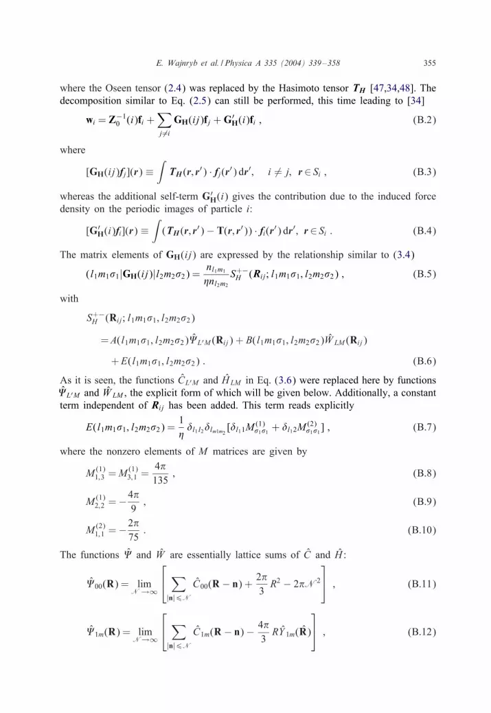
where the Oseen tensor (2.4) was replaced by the Hasimoto tensor TH [47,34,48]. Thedecomposition similar to Eq. (2.5) can still be performed, this time leading to [34]

wi = Z−10 (i)fi +

∑j �=i

GH(ij)fj +G′H(i)fi ; (B.2)

where

[GH(ij)fj](r) ≡∫TH (r; r′) · fj(r′) dr′; i = j; r∈ Si ; (B.3)

whereas the additional self-term G′H(i) gives the contribution due to the induced force

density on the periodic images of particle i:

[G′H(i)fi](r) ≡

∫(TH (r; r′) − T(r; r′)) · fi(r′) dr′; r∈ Si : (B.4)

The matrix elements of GH(ij) are expressed by the relationship similar to (3.4)

(l1m1�1|GH(ij)|l2m2�2) =nl1m1

�nl2m2

S+−H (Rij; l1m1�1; l2m2�2) ; (B.5)

with

S+−H (Rij; l1m1�1; l2m2�2)

=A(l1m1�1; l2m2�2)7L′M (Rij) + B(l1m1�1; l2m2�2)W LM (Rij)

+E(l1m1�1; l2m2�2) : (B.6)

As it is seen, the functions CL′M and H LM in Eq. (3.6) were replaced here by functions7L′M and W LM , the explicit form of which will be given below. Additionally, a constantterm independent of Rij has been added. This term reads explicitly

E(l1m1�1; l2m2�2) =1�)l1l2)lm1m2

[)l11M(1)�1�1 + )l12M

(2)�1�1 ] ; (B.7)

where the nonzero elements of M matrices are given by

M (1)1;3 =M (1)

3;1 =4�135

; (B.8)

M (1)2;2 = −4�

9; (B.9)

M (2)1;1 = −2�

75: (B.10)

The functions 7 and W are essentially lattice sums of C and H :

700(R) = limN→∞

∑|n|6N

C00(R− n) + 2�3

R2 − 2�N2

; (B.11)

71m(R) = limN→∞

∑|n|6N

C1m(R− n) − 4�3

RY 1m(R)

; (B.12)

356 E. Wajnryb et al. / Physica A 335 (2004) 339–358

7lm(R) = limN→∞

∑|n|6N

Clm(R− n); l= 2; 3; : : : ; (B.13)

W 2m(R) = limN→∞

∑|n|6N

H 2m(R− n) − 8�15

R2Y 2m(R)

; (B.14)

W lm(R) = limN→∞

∑|n|6N

H lm(R− n); l= 3; 4; : : : ; (B.15)

where n, with integer components nx; ny; nz, denotes a lattice point.Finally, the matrix elements of G′

H(ij) are given by

(l1m1�1|G′H(ij)|l2m2�2) =

nl1m1

� nl2m2

(A(l1m1�1; l2m2�2) L′M

+B(l1m1�1; l2m2�2)wLM + E(l1m1�1; l2m2�2)

); (B.16)

where the coe7cients and w can be expressed as

LM = 7′LM (0) ; (B.17)

wLM = W ′LM (0) ; (B.18)

with the prime indicating that in the sums in Eqs. (B.11)–(B.15) the n= 0 term is tobe omitted.Since we have already derived the spherical gradient rules for functions C and H

in Eqs. (3.24) and (3.27), now we can apply these rules to the lattice sums (B.11),(B.12), (B.13) and (B.14), (B.15), and @nally obtain the gradient formulas for 7and W

7LM ;m(R) = (−1)m+1 (L − M + m+ 1)!(L − M)!(1 − m)!

7L+1;M−m(R)

− 4�3

2m)L1)Mm ; (B.19)

W LM ;m(R) =2(L+M)!

(2L+ 1)(L+M − m − 1)!(1 − m)!7L−1;M−m(R)

+ (−1)m+1 (2L − 1)(L − M + m+ 1)!(2L+ 1)(L − M)!(1 − m)!

W L+1;M−m(R) ; (B.20)

which allows us to @nd the gradient of GH and then the divergence of mobility matrixin a complete analogy with the in@nite space case.

References

[1] P.N. Pusey, Colloidal suspensions, in: J.P. Hansen, D. Levesque, J. Zinn-Justin (Eds.), Liquids, Freezingand Glass Transition, Elsevier, Amsterdam, 1991, pp. 763–942.

E. Wajnryb et al. / Physica A 335 (2004) 339–358 357

[2] L. Durlofsky, J.F. Brady, G. Bossis, Dynamic simulation of hydrodynamically interacting particles,J. Fluid Mech. 180 (1987) 21.

[3] A.J.C. Ladd, Hydrodynamic interactions in a suspension of spherical particles, J. Chem. Phys. 88 (1988)5051.

[4] B. Cichocki, B.U. Felderhof, R. Schmitz, Hydrodynamic interactions between two spherical particles,Physico Chem. Hydrodyn. 10 (3) (1988) 383.

[5] B. Cichocki, B.U. Felderhof, K. Hinsen, E. Wajnryb, J. Blawzdziewicz, Friction and mobility of manyspheres in Stokes 3ow, J. Chem. Phys. 100 (5) (1994) 3780.

[6] K. Hinsen, Hydrolib: a library for the evaluation of hydrodynamic interactions in colloidal suspensions,Comp. Phys. Comm. 88 (1995) 327.

[7] B. Cichocki, R.B. Jones, R. Kutteh, E. Wajnryb, Friction and mobility for colloidal spheres in Stokes3ow near a boundary: the multipole method and applications, J. Chem. Phys. 112 (5) (2000) 2548.

[8] D.L. Ermak, J.A. McCammon, Brownian dynamics with hydrodynamic interactions, J. Chem. Phys. 69(4) (1978) 1352.

[9] E. Dickinson, Brownian dynamics with hydrodynamics interactions: the application to protein di6usionalproblems, Chem. Soc. Rev. 14 (1985) 421.

[10] E. Dickinson, S.A. Allison, J.A. McCammon, Brownian dynamics with rotation-translation coupling,J. Chem. Soc. Faraday Trans. 2 81 (1985) 591.

[11] G.C. Ansell, E. Dickinson, M. Ludvigson, Brownian dynamics of colloidal-aggregate rotation anddissociation in shear 3ow, J. Chem. Soc. Faraday Trans. 2 81 (1985) 1269.

[12] G.C. Ansell, E. Dickinson, Brownian dynamics simulation of the fragmentation of a large colloidal 3ocin simple shear 3ow, J. Colloid Interface Sci. 110 (1986) 73.

[13] G.C. Ansell, E. Dickinson, Sediment formation by Brownian dynamics simulation: e6ect of colloidaland hydrodynamic interactions on the sediment structure, J. Chem. Phys. 85 (1986) 4079.

[14] W. van Megen, I.K. Snook, Brownian dynamics simulation of concentrated charge stabilized dispersions.Self di6usion, J. Chem. Soc. Faraday Trans. 80 (2) (1984) 383.

[15] K. Gaylor, I. Snook, W. van Megen, Comparison of Brownian dynamics with photon correlationspectroscopy of strongly interacting colloidal particles, J. Chem. Phys. 75 (1981) 1682.

[16] P. Szymczak, B. Cichocki, Memory function for collective di6usion of interacting Brownian particles,Europhys. Lett. 59 (3) (2002) 465.

[17] W. Hess, R. Klein, Generalized hydrodynamics of systems of Brownian particles, Adv. Phys. 32 (2)(1983) 173.

[18] B.J. Ackerson, Correlations for interacting Brownian particles. II, J. Chem. Phys. 69 (2) (1978) 684.[19] S. Kim, S.J. Karilla, Microhydrodynamics, Butterworth–Heinemann, Boston, 1991.[20] R.G. Cox, H. Brenner, E6ect of @nite boundaries on the Stokes resistance of an arbitrary particle. Part 3.

Translation and rotation, J. Fluid. Mech. 28 (1967) 391.[21] P. Mazur, D. Bedeaux, Generalization of Faxen’s theorem to nonsteady motion of a sphere through an

incompressible 3uid in arbitrary 3ow, Physica 76 (1974) 235.[22] B.U. Felderhof, Force density induced on a sphere in linear hydrodynamics I. Fixed sphere, stick

boundary conditions, Physica A 84 (1976) 557.[23] R. Schmitz, B.U. Felderhof, Mobility matrix for two spherical particles with hydrodynamic interaction,

Physica A 116 (1982) 163.[24] U.A. Ladyzhenskaya, The Mathematical Theory of Viscous Incompressible Flow, Gordon and Breach,

New York, 1963.[25] C. Pozrikidis, Boundary Integral and Singularity Methods for Linearized Viscous Flow, Cambridge

University Press, Cambridge, MA, 1992.[26] P. Mazur, W. van Saarlos, Many-sphere hydrodynamic interactions and mobilities in a suspension,

Physica A 115 (1982) 21.[27] B.U. Felderhof, Many-body hydrodynamic interactions in suspensions, Physica A 151 (1988) 1.[28] B. Cichocki, M.L. Ekiel-Jezewska, E. Wajnryb, Lubrication corrections for three-particle contribution

to short-time self-di6usion coe7cients in colloidal dispersions, J. Chem. Phys. 111 (1999) 3265.[29] D.J. Je6rey, Y. Onishi, Calculation of the resistance and mobility function for two unequal rigid spheres

in low-Reynolds-number 3ow, J. Fluid Mech. 139 (1984) 261.

358 E. Wajnryb et al. / Physica A 335 (2004) 339–358

[30] B.U. Felderhof, R.B. Jones, Displacement theorems for spherical solutions of the linear Navier-Stokesequations, J. Math. Phys. 30 (2) (1989) 339.

[31] J.A.R. Coope, R.F. Snider, Irreducible cartesian tensors. II. General formulation, J. Math. Phys. 11 (3)(1970) 1003.

[32] D. Forster, Hydrodynamic Fluctuations, Broken Symmetry and Correlation Functions, W.A. Benjamin,Inc., New York, 1975.

[33] E.R. Smith, I.K. Snook, W. van Megen, Hydrodynamic interactions in Brownian dynamics. I. Periodicboundary conditions for computer simulations, Physica A 143 (1987) 441.

[34] B.U. Felderhof, Hydrodynamic interactions in suspensions with periodic boundary conditions, PhysicaA 159 (1989) 1.

[35] R. Zwanzig, N.K. Ailawadi, Statistical error due to @nite time averaging in computer experiments, Phys.Rev. 182 (1) (1969) 280.

[36] B.J. Alder, T.E. Wainwright, Studies in molecular dynamics. I. General method, J. Chem. Phys. 31(1959) 459.

[37] B.J. Alder, T.E. Wainwright, Studies in molecular dynamics. II. Behaviour of a small number of elasticspheres, J. Chem. Phys. 33 (1960) 1439.

[38] M.P. Allen, D.J. Tildesley, Computer Simulation of Liquids, Clarendon Press, Oxford, 1987.[39] D. Frenkel, B. Smit, Understanding Molecular Simulation: From Algorithms to Applications, Academic

Press, San Diego, 1996.[40] B.J. Ackerson, L. Fleishmann, Correlations for dilute hard core suspensions, J. Chem. Phys. 76 (1982)

2675.[41] G. NXagele, On the dynamics and structure of charge-stabilized suspensions, Phys. Rep. 272 (1996) 215.[42] B. Cichocki, B.U. Felderhof, Time-dependent self-di6usion coe7cient of interacting Brownian particles,

Phys. Rev. A 44 (1991) 6551.[43] B. Cichocki, B.U. Felderhof, Slow dynamics of linear relaxation systems, Physica A 211 (1994) 165.[44] M. Medina-Noyola, Long-time self-di6usion in concentrated colloidal dispersions, Phys. Rev. Lett. 60

(1988) 2705.[45] A.J.C. Ladd, Hydrodynamic transport coe7cients of random dispersions of hard spheres, J. Chem. Phys.

93 (5) (1990) 3484.[46] A.R. Edmonds, Angular Momentum in Quantum Mechanics, Princeton University. Press, Princeton, NJ,

1960.[47] H. Hasimoto, On the periodic fundamental solutions of the Stokes equations and their application to

viscous 3ow past a cubic array of spheres, J. Fluid. Mech. 5 (1959) 317.[48] B. Cichocki, B.U. Felderhof, K. Hinsen, Periodic fundamental solution of the linear Navier–Stokes

equation, Physica A 159 (1989) 19.