Constraint relations in two-tensor gravity1

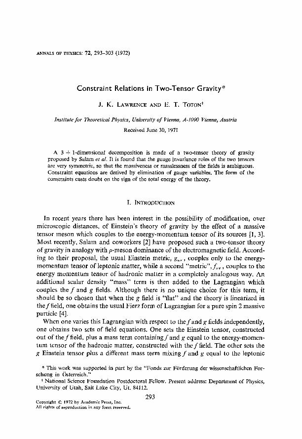
ANNALS OF PHYSICS: 72, 293-303 (1972)

Constraint Relations in Two-Tensor Gravity*

J. K. LAWRENCE AND E. T. TOTON’

Institute for Theoretical Physics, University of Vienna, A-1090 Vienna, Austria

Received June 30, 1971

A 3 + l-dimensional decomposition is made of a two-tensor theory of gravity proposed by Saiam et al. It is found that the gauge invariance roles of the two tensors are very symmetric, so that the massiveness or masslessness of the fields is ambiguous. Constraint equations are derived by elimination of gauge variables. The form of the constraints casts doubt on the sign of the total energy of the theory.

I. INTR~DUCTJON

In recent years there has been interest in the possibility of modification, over microscopic distances, of Einstein’s theory of gravity by the effect of a massive tensor meson which couples to the energy-momentum tensor of its sources [l, 31. Most recently, Salam and coworkers [2] have proposed such a two-tensor theory of gravity in analogy with p-meson dominance of the electromagnetic field. Accord- ing to their proposal, the usual Einstein metric, g,, , couples only to the energy- momentum tensor of leptonic matter, while a second “metric”,fUV, couples to the energy momentum tensor of hadronic matter in a completely analogous way. An additional scalar density “mass” term is then added to the Lagrangian which couples the f and g fields. Although there is no unique choice for this term, it should be so chosen that when the g field is “flat” and the theory is linearized in theffield, one obtains the usual Fierz form of Lagrangian for a pure spin 2 massive particle [4].

When one varies this Lagrangian with respect to the f and g fields independently, one obtains two sets of field equations. One sets the Einstein tensor, constructed out of theffield, plus a mass term containingfand g equal to the energy-momentum tensor of the hadronic matter, constructed with theffield. The other sets the g Einstein tensor plus a different mass term mixing f and g equal to the leptonic

* This work was supported in part by the “Fonds zur Forderung der wissenschaftlichen For- schung in ijsterreich.”

+ National Science Foundation Postdoctoral Fellow. Present address: Department of Physics, University of Utah, Salt Lake City, Ut. 84112.

293 Copyright 0 1972 by Academic Press, Inc. All rights of reproduction in any form reserved.

294 LAWRENCE AND TOTON

energy-momentum tensor, constructed with the g field. Thus we see that neither the g nor the f fields play the role of a pure massless or pure massive state. In the analogous electromagnetic case, because of the linearity of the field equations, it is possible to choose two linear combinations of the y and p fields, such that one field, “y”, satisfies a massless field equation and thus enjoys all the rights and privileges of a massless field, including gauge invariance. The other, “p”, field obeys a field equation with mass and is not gauge invariant, a gauge condition being imposed upon it by the field equations due to the presence of the mass term. In the linearizedf-g theory it also seems possible to perform such a “diagonaliza- tion” of the Lagrangian and thus sort out the gauge invariance properties of the two fields. For the full, nonlinear f-g theory, however, this is not the case. One cannot choose a combination of thef’s and g’s such that it will obey a normal, massless Einstein equation. There is no field which fills the position of a pure massless metric field with full coordinate invariance and no corresponding massive, completely noninvariant field.

That the field equations impose just the right number (four) of gauge conditions on the f and g fields is easy to show from a simple argument. If one covariantly differentiates the “hadronic” field equations with respect to the f field and the “leptonic” with respect to the g field, one has that the Einstein tensor terms vanish due to the Bianchi identities and that the energy-momentum tensor terms vanish due to the equations of motion of the matter. One is then apparently left with the eight conditions that the f and g covariant derivatives of the respective mass terms must vanish. It follows, however, from the fact that the total Lagrangian is a scalar density, that the sum of these two covariant derivatives must vanish identically, and we are just left with the desired four imposed gauge conditions.

While the fact that we have the correct number of gauge conditions is reassuring, their mathematical complexity makes it very difficult to use them to simplify the field equations. In the p-meson case, the imposed gauge condition is very simple, being just a Lorentz gauge condition. This is then easy to substitute into the field equations to eliminate a field variable, namely the longitudinal component of the p” vector field. Although the case of the two-tensor theory is formally analogous, the nonlinear complexity of the gauge conditions and the field equations makes such a simplification seem hopeless. There exists, however, a systematic approach to such problems, and this is to make the 3 + l-dimensional decomposition of the two-tensor theory into canonical form, in analogy with the canonical form for general relativity of Arnowitt, Deser and Misner (ADM). A complete list of references to this work is contained in Ref. [5]. This reduction is equivalent to that used in Lorentz covariant field theories when one wishes to go to the canonical form by eliminating the extra constraint field variables which must be added to the minimal set of dynamical variables to achieve manifest covariance. Thus, in the case of general relativity, the time coordinate is distinguished from the three

TWO-TENSOR GRAVITY 295

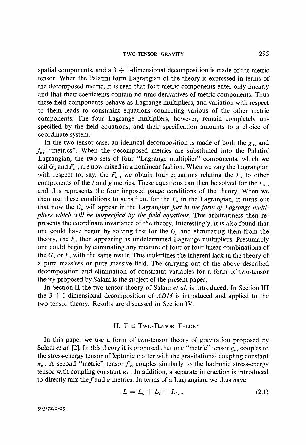
spatial components, and a 3 + l-dimensional decomposition is made of the metric tensor. When the Palatini form Lagrangian of the theory is expressed in terms of the decomposed metric, it is seen that four metric components enter only linearly and that their coefficients contain no time derivatives of metric components. Thus these field components behave as Lagrange multipliers, and variation with respect to them leads to constraint equations connecting various of the other metric components. The four Lagrange multipliers, however, remain completely unspecified by the field equations, and their specification amounts to a choice of coordinate system.

In the two-tensor case, an identical decomposition is made of both the g,, and f “metrics”. When the decomposed metrics are substituted into the Palatini iigrangian, the two sets of four “ Lagrange multiplier” components, which we call G, and FU , are now mixed in a nonlinear fashion. When we vary the Lagrangian with respect to, say, the FU , we obtain four equations relating the F, to other components of thefand g metrics. These equations can then be solved for the F, , and this represents the four imposed gauge conditions of the theory. When we then use these conditions to substitute for the F, in the Lagrangian, it turns out that now the G, will appear in the Lagrangian just in the form of Lagrange multipliers which will be unspecz$ed by the field equations. This arbitrariness then represents the coordinate invariance of the theory. Interestingly, it is also found that one could have begun by solving first for the G,, and eliminating them from the theory, the F, then appearing as undetermined Lagrange multipliers. Presumably one could begin by eliminating any mixture of four or four linear combinations of the G, or FU with the same result. This underlines the inherent lack in the theory of a pure massless or pure massive field. The carrying out of the above described decomposition and elimination of constraint variables for a form of two-tensor theory proposed by Salam is the subject of the present paper.

In Section II the two-tensor theory of Salam et al. is introduced. In Section III the 3 + l-dimensional decomposition of ADM is introduced and applied to the two-tensor theory. Results are discussed in Section IV.

IT. THE TWO-TENSOR THEORY

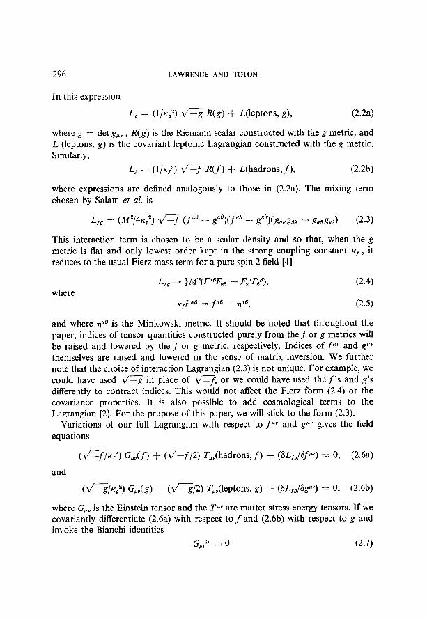
In this paper we use a form of two-tensor theory of gravitation proposed by Salam et al. [2]. In this theory it is proposed that one “metric” tensor g,, couples to the stress-energy tensor of leptonic matter with the gravitational coupling constant Q, . A second “metric” tensor f,, couples similarly to the hadronic stress-energy tensor with coupling constant Kf . In addition, a separate interaction is introduced to directly mix thefand g metrics. In terms of a Lagrangian, we thus have

L = L, i- Lf f LfB. (2.1)

595/741-19


In this expression

L, = (l/~,~> v’?j R(g) + L(leptons, g), (2.2a)

where g = det g,, , R(g) is the Riemann scalar constructed with the g metric, and L (leptons, g) is the covariant leptonic Lagrangian constructed with the g metric. Similarly,

Lf = (l/$) q R(f) + L(hadrons,f), (2.2b)

where expressions are defined analogously to those in (2.2a). The mixing term chosen by Salam et al. is

L,p. = (M2/4Kf2) d\/-f wB - &@>(f”” - P~(g~lcg8A - &f&J (2.3)

This interaction term is chosen to be a scalar density and so that, when the g metric is flat and only lowest order kept in the strong coupling constant K~, it reduces to the usual Fierz mass term for a pure spin 2 field [4]

L,, + @4”(Fa8FmB - Fa”Fop), (2.4) where

,+a0 = f”B - rln8, (2.5)

and where ~“8 is the Minkowski metric. It should be noted that throughout the paper, indices of tensor quantities constructed purely from the f or g metrics will be raised and lowered by the f or g metric, respectively. Indices off“” and g”” themselves are raised and lowered in the sense of matrix inversion. We further note that the choice of interaction Lagrangian (2.3) is not unique. For example, we could have used 4-g in place of q\/-f or we could have used the f’s and g’s differently to contract indices. This would not affect the Fierz form (2.4) or the covariance properties. It is also possible to add cosmological terms to the Lagrangian [2]. For the prupose of this paper, we will stick to the form (2.3).

Variations of our full Lagrangian with respect to fuV and g”” gives the field equations

(d~/G> GUY(f) + (d?/2) T,,,@adrons,f) + @Lfgl~fpy) = 0, (2.W and

(d--g/~,~) G,,(g) + (2/?/2) T,,(leptons, g) + @Lf,/W”) = 0, (2.6b)

where GUY is the Einstein tensor and the TuY are matter stress-energy tensors. If we covariantly differentiate (2.6a) with respect to .f and (2.6b) with respect to g and invoke the Bianchi identities

GFV;” GZ 0 (2.7)


and the matter equations of motion

T :vr() UY 3

we are apparently left with the eight conditions on the fields

(2.8)

and VfqsLf*/Efq = 0 (2.9a)

v,q3Lf,/sg”“) = 0. (2.9b)

It follows, however, from the fact that Lf, is a scalar density, that the sum of the two expressions (2.9) must vanish identically. Thus we are correctly left with four “gauge” conditions on the f’s and g’s, just corresponding to the one Lorentz gauge condition which is imposed on massive vector fields by the presence of a mass term in the field equations.

Our situation differs from the case of p-meson dominance of electromagnetism because of the nonlinear nature of the theory. In the p-y theory, it is possible to choose linear combinations of the p and y fields such that one represents a purely massless field with full gauge invariance while the other is a purely massive field with a Lorentz gauge condition imposed by the mass term. In our case no such recombinations off and g can be made, and so the two fields remain ambiguous with respect to being massless or massive fields. As we will see later, we can choose to impose the gauge conditions on either four components off or of g, or indeed on mixtures of the two. When this is done, there remain always four completely unspecified components off or g or a mixture.

Although we have been able to satisfy ourselves that the right number of gauge restrictions are present in the theory, the obvious complexity of the conditions (2.9) makes them useless for eliminating the constrained field variables from the theory. To achieve this, it will be necessary to make use of a systematic approach to this problem which was developed for general relativity.

III. THE 3 + I-DIMENSIONAL DECOMPOSITION

The following approach to general relativity was developed by Amowitt, Deser, and Misner (ADM) in a program to put that theory in canonical form, analogous to the canonical form of usual Lorentz covariant field theories [S]. The purpose of such a procedure is to discover the true dynamical modes of the theory by system- atically eliminating the extra constraint and gauge variables which must be included to give the theory a manifestly covariant form. One begins this task by separating the time coordinate from the others and making a “3 + l-dimensional decomposition” of the fields.


In this paper, we use the notations and conventions of Ref. [5]. In particular, the Minkowski metric has signature (- 1, + 1, + 1, + 1). Note that this and the sign convention used for the Riemann tensor differ from reference [2]. In the case of general relativity ADM make the definitions

gi5 = “gij , G = (-4g”“)-‘/2, Gi s 4goi 3

P(g) = 2/-“g (“r;., - g,, 4r,o,grp gip‘giq.

(3.la)

(3.lb)

In the remainder of the paper, all four-dimensional quantities are marked with the upper prefix 4, so that those unmarked are three-dimensional. Thus gii in (3. lb) is the matrix inverse of g, . We can now write the full metric in the form

“g,o = -(G2 - GiGi), (3.2)

where Gi = g i?G. 3 9 and

Further,

4gYi = Gi/G2, 4goo = -I/@,

4gii = gii _ GiGj/Ga.

d-“g= G d;.

(3.3a)

(3.3b)

(3.4)

In terms of these quantities, the sourceless Lagrangian of general relativity becomes

L = d-4~ = -#giiSO - GR" - GiRi $- (divergence), (3.5)

where

RO 3 -& [3R + g-l&r2 - &7~~~)], (3.6a)

Ri z -2+i I5 . (3.6b)

Here 3R is the curvature scalar formed from the spatial metric gi,, 1 indicates covariant differentiation with respect to this metric, and spatial indices are raised and lowered by gij and gii . Also z- = rii.

When the divergence term is discarded, it is clear that the four quantities G,, = G, Gi appear only linearly in the Lagrangian, i.e., in the form of Lagrange multipliers. Thus the G, will be completely undetermined by the field equations, their choice corresponding to a choice of coordinate frame. Varying the Lagrangian with respect to the G, produces the four constraint equations

Ru = 0. (3.7)


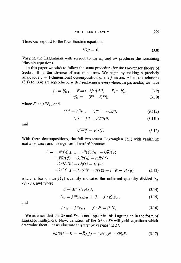
These correspond to the four Einstein equations

4Gw0 = 0. (3.8)

Varying the Lagrangian with respect to the gij and rrii produces the remaining Einstein equations.

In this paper we wish to follow the same procedure for the two-tensor theory of Section II in the absence of matter sources. We begin by making a precisely analogous 3 + l-dimensional decomposition of the f metric. All of the relations (3.1) to (3.4) are reproduced with f replacing g everywhere. In particular, we have

.fij = xi, &’ s (-4j”“)-l/2, Fi s “foi , (3.9) yoo = -(F2 - FiFi)p (3.10)

where Fi = fijFj , and

4foi = p/p, itff’o = -l/$‘s, (3.11a)

4f ij = f ij _ t;ip’/F2 , (3.1 lb)

and

d/-“f= Fd?. (3.12)

With these decompositions, the full two-tensor Lagrangian (2.1) with vanishing matter sources and divergences discarded becomes

L = -+‘(g)gii,, - fii’(f)Lj,o - GE’(g)

-FF( f) - G,Ri( g) - FiKi( f)

-2aNij(F” - Gi)(l;” - G’)/F

-2a( f . g - 3) G2/F - aF( 12 - f . N - 3f. g), (3.13)

where a bar on an f(g) quantity indicates the unbarred quantity divided by K~~(K~~), and where

a = M2 @//4~~~, (3.14)

Nj E f mngmignj + (3 - f * g) gij 7 (3.15)

and f * g E f 2gij ; feN-fijNii. (3.16)

We now see that the GU and F” do not appear in this Lagrangian in the form of Lagrange multipliers. Now, variation of the GU or Fu will yield equations which determine them. Let us illustrate this first by varying the P.

6L/6Fi = 0 = -Ri( f) - 4aN,(F’ - G’)/F, (3.17)


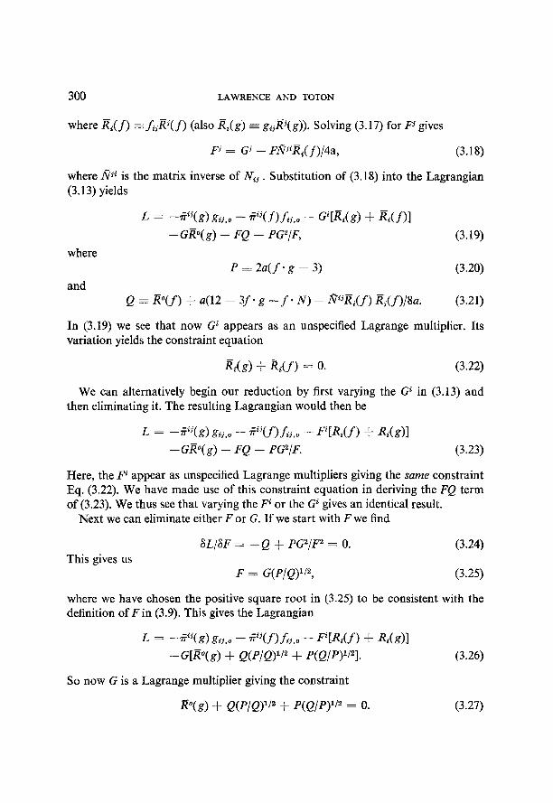
where R,(j) =f&Rj(j) (also Bi(g) = g#( g)). Solving (3.17) for Fj gives

P = Gj - FNjiai( j)/4a, (3.18)

where #i is the matrix inverse of Ni, . Substitution of (3.18) into the Lagrangian (3.13) yields

where

and

L = -+j(g) gii.0 - fij( j)J;j,o - Q[Ri(g) + Bi( j)]

- Gi+‘( g) - FQ - PG2/F,

P-2a(f*g-3)

(3.19)

(3.20)

Q E P(f) + a(12 - 3j * g - f * N) - ??ja,(j) &(f)/Sa. (3.21)

In (3.19) we see that now Gi appears as an unspecified Lagrange multiplier. Its variation yields the constraint equation

K(g) + K(f) = 0. (3.22)

We can alternatively begin our reduction by first varying the Gi in (3.13) and then eliminating it. The resulting Lagrangian would then be

L = -+(g) gii,o - S(f)j& - Fi[Ri(f) + l&(g)]

- GR”( g) - FQ - PG2/F. (3.23)

Here, the F+ appear as unspecified Lagrange multipliers giving the same constraint Eq. (3.22). We have made use of this constraint equation in deriving the FQ term of (3.23). We thus see that varying the Pi or the Gi gives an identical result,

Next we can eliminate either F or G. If we start with F we find

This gives us 6Lj6F = -Q + PG2/F2 = 0.

F = G(P/Q)‘/“,

(3.24)

(3.25)

where we have chosen the positive square root in (3.25) to be consistent with the definition of F in (3.9). This gives the Lagrangian

L = -S(g) gij,o - +(f)fij,o - Fi[R,(f) + It&)]

-G[a’(g> + Q(P/QY2 + P(Q/P)““l. (3.26)

So now G is a Lagrange multiplier giving the constraint

a”(g) + Q(P/Q)‘i2 + P(Q/P)‘l” = 0. (3.27)


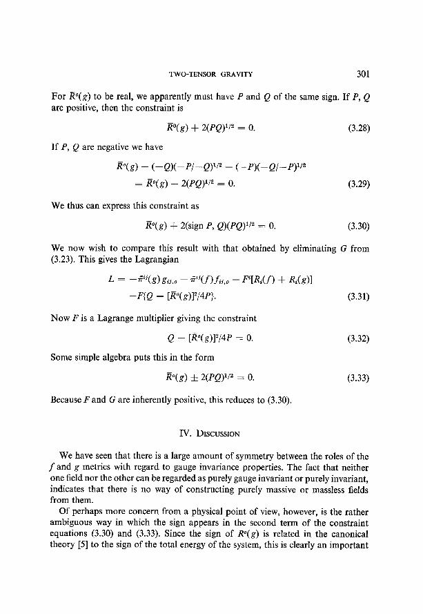
For P(g) to be real, we apparently must have P and Q of the same sign. If P, Q are positive, then the constraint is

WO(g) + 2(PQ)‘/” = 0. (3.28)

If P, Q are negative we have

B”(g)-(-Q)(-P/-Q)lj2 -(-P)(-Q/-P)“‘”

= RO(g) - 2(PQ)“” = 0. (3.29)

We thus can express this constraint as

P(g) + 2(sign P, Q)(PQ)‘/” = 0. (3.30)

We now wish to compare this result with that obtained by eliminating G from (3.23). This gives the Lagrangian

L = -?iyg)gij,, - ??“j(f)J;:j,o - Fi[Ri(f) + R,(g)1

-F{Q - [~W12/‘W. (3.31)

Now F is a Lagrange multiplier giving the constraint

Q - [p(g)12/4P = 0. (3.32)

Some simple algebra puts this in the form

R”(g) & 2(PQ)“” = 0. (3.33)

Because F and G are inherently positive, this reduces to (3.30).

IV. DISCUSSION

We have seen that there is a large amount of symmetry between the roles of the f and g metrics with regard to gauge invariance properties. The fact that neither one field nor the other can be regarded as purely gauge invariant or purely invariant, indicates that there is no way of constructing purely massive or massless fields from them.

Of perhaps more concern from a physical point of view, however, is the rather ambiguous way in which the sign appears in the second term of the constraint equations (3.30) and (3.33). Since the sign of P(g) is related in the canonical theory [5] to the sign of the total energy of the system, this is clearly an important


matter. From these constraint equations it is not clear whether the sign is imposed by the field equations or whether it must be chosen as an initial condition. In the latter case, it is not clear whether the choice will be preserved in time by the field equations. It is hoped that these questions can be answered in the near future in the process of solving the equations.

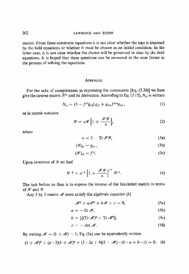
APPENDIX

For the sake of completeness in expressing the constraints [Eq. (3.30)] we here give the inverse matrix mij and its derivation. According to Eq. (3.15), Nij is written

Nij = (3 - f%d gij + gimP%j , (1)

or in matrix notation

N=&[l+q], (2)

where

a:=3-TrP9, (34

6% = gii 3 W

(3F)ij = fii* (3c)

Upon inversion of N we find

N-1 = a-1 1 + ??.m -' 9-l. 1 (4) a

The task before us then is to express the inverse of the bracketed matrix in terms of 9 and 9.

Any 3 by 3 matrix J/Z must satisfy the algebraic equation [6]

A3 + aA + bJi’ + c = 0, (54

a = -Tr&, (5b)

b = $[(Tr JL+‘)~ - Tr AZ], (5c)

c = -detJZ. (54

By writing J&’ = (1 + JH) - 1, Eq. (5a) can be equivalently written

(1 + J&‘)” + (a - 3)(1 + J!)” + (3 -2a + b)(l + A) - (1 - a + b - c) = 0. (6)


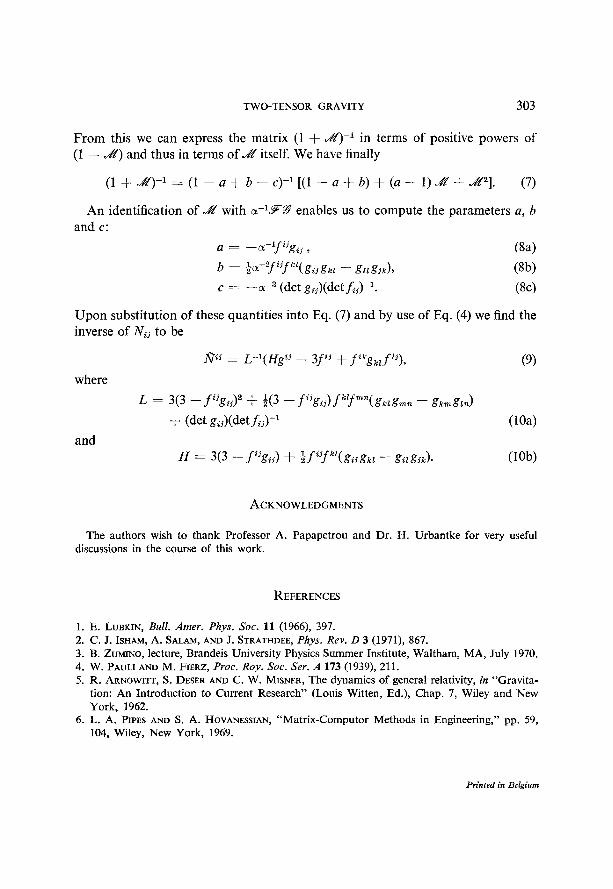
From this we can express the matrix (1 + A)-’ in terms of positive powers of (I + M) and thus in terms of&! itself. We have finally

(1 + J&C!-’ = (1 - a + b - c)-’ [(I - a + b) + (a - 1) Jz + .&PI. (7)

An identification of ~2’ with cu-lF% enables us to compute the parameters a, b and c:

a = --“-lfijgij , (84 b = &a-‘f i’f kz( gij gk, - gi, g.jk), @b) c = -c3 (det g,J(detfi&l. PC)

Upon substitution of these quantities into Eq. (7) and by use of Eq. (4) we find the inverse of Nij to be

where

&lij = L-l(Hgij _ 3f ij + f ikgkl f Ii), (9)

and

L = 3(3 - f i’gij)” + $(3 - f “‘gij)f kffmn(gklgncn - gkmg,n)

+ @et gij)(detf;j)-l (104

H = 3(3 -f'jgij) $ $f'jf""(gijgk, - gilgjk). (lob)

ACKNOWLEDGMENTS

The authors wish to thank Professor A. Papapetrou and Dr. H. Urbantke for very useful discussions in the course of this work.

REFERENCES

1. E. LUEKIN, BUN. Amer. Phys. Sot. 11 (1966), 397. 2. C. J. ISHAM, A. SALAM, AND .I. STRATHDEE, Phys. Rev. D 3 (1971), 867. 3. B. ZUMINO, lecture, Brandeis University Physics Summer Institute, Waltham, MA, July 1970. 4. W. PAULI AND M. F~ERZ, Proc. Roy. Sot. Ser. A 173 (1939), 211. 5. R. ARNO~~~T, S. DESER AND C. W. MISNER, The dynamics of general relativity, in “Gravita-

tion: An Introduction to Current Research” (Louis Witten, Ed.), Chap. 7, Wiley and New York, 1962.

6. L. A. PINES AND S. A. HOVANESSIAN, “Matrix-Computer Methods in Engineering,” pp. 59, 104, Wiley, New York, 1969.

Constraint relations in two-tensor gravity1

Documents

Transcript of Constraint relations in two-tensor gravity1