Diffeomorphic Matching of Diffusion Tensor Images

Yan Cao,Center for Imaging Science, Johns Hopkins University

Michael I. Miller,Center for Imaging Science, Johns Hopkins University

Susumu Mori,Department of Radiology and Kennedy Krieger Institute, Johns Hopkins University, School ofMedicine

Raimond L. Winslow, andCenter for Cardiovascular Bioinformatics & Modeling and the Whitaker Biomedical EngineeringInstitute, Johns Hopkins University

Laurent YounesCenter for Imaging Science, Johns Hopkins University

Yan Cao: yan@cis.jhu.edu; Michael I. Miller: mim@cis.jhu.edu; Susumu Mori: susumu@mri.jhu.edu; Raimond L.Winslow: rwinslow@bme.jhu.edu; Laurent Younes: younes@cis.jhu.edu

AbstractThis paper proposes a method to match diffusion tensor magnetic resonance images (DT-MRI)through the large deformation diffeomorphic metric mapping of tensor fields on the imagevolume, resulting in optimizing for geodesics on the space of diffeomorphisms connecting twodiffusion tensor images. A coarse to fine multi-resolution and multi-kernel-width scheme isdetailed, to reduce both ambiguities and computation load. This is illustrated by numericalexperiments on DT-MRI brain and images.

1. IntroductionDiffusion Tensor Magnetic Resonance Imaging (DT-MRI) is a non-invasive technique thatmeasures the diffusion of water molecules in biological tissues [16,14,20,9]. Diffusion refersto the random translational movement of molecules (also called Brownian motion). The rateand direction of the movement is closely related to the structural anisotropy of the medium,hence it can be used to infer the tissue micro structure. Diffusion is describedmathematically by a symmetric second order tensor. Orientation of the principal eigenvectorof the diffusion tensor is known to align with fiber tracts [16,20]. DT-MRI is rapidly gainingimportance in neuroscience and other fields but tools for exploring and analyzing DT-MRIdata are still not widely available.

Image registration is inevitable whenever images acquired from different subjects, atdifferent times, or from different scanners need to be combined or compared for analysis orvisualization. Alexander and Gee [1] adapted the multi-resolution elastic matching algorithmusing tensor similarity measures for matching DT-MRIs. Tensor reorientation is notincluded in the energy function, but tensors are reoriented in each iteration according to theestimated displacement field. Ruiz-Alzola [19] proposed a unified framework forregistration of medical volumetric multi-valued data by matching local areas with highstructure. Local structure is detected by measuring “cornerness”. Then the Kriging estimatorwas used to interpolate the displacement field in the remaining areas. Tensor reorientation is

NIH Public AccessAuthor ManuscriptProc IEEE Comput Soc Conf Comput Vis Pattern Recognit. Author manuscript; available inPMC 2010 August 12.

Published in final edited form as:Proc IEEE Comput Soc Conf Comput Vis Pattern Recognit. 2006 July 5; 2006: 67. doi:10.1109/CVPRW.2006.65.

NIH

-PA

Author M

anuscriptN

IH-P

A A

uthor Manuscript

NIH

-PA

Author M

anuscript

performed after the registration. Guimond et al. [11] proposed a deformable registrationmethod using tensor characteristics that are invariant to rigid transformations to avoid thecomplexity of tensor reorientation. The invariants used in their experiments are the tensoreigenvalues. Rohde et al. [18] proposed an intensity based registration method capable ofperforming affine and nonlinear registration of multi-channel images. The multi-channelsimilarity measure considered both the similarity between same-index image channels andthe similarity between image channels with different index. But tensor reorientation isperformed after affine registration and after the nonlinear registration is complete. Zhang etal [21] proposed a piecewise local affine registration algorithm. Leemans et al [12] proposedan affine multi-channel matching method for DT-MRIs based on mutual information. TheDiffusion Weighted Images was used as the channels.

This paper proposes a method to match diffusion tensor magnetic resonance images throughan extension of the Large Deformation Diffeomorphic Metric Mapping (LD-DMM)framework [5] to this type of dataset, resulting in optimizing for geodesics on the space ofdiffeomorphisms connecting two tensor fields. In [7], LDDMM framework was extended tomatching vector fields. In the paper, we extends it further to the full tensor fields.Establishing this methodology continues our efforts on establishing the construction andcomputation of metric spaces for studying anatomical structures. Our method includestensor reorientation in the optimization, hence the measure of difference is calculatedcorrectly during the optimization. Convergence of the algorithm is guaranteed.

2. Formulation of the ProblemIn our approach, anatomy is modeled as a deformable template. The images are defined onan open bounded set and are viewed as the orbit under the diffeomorphic transformations Gacting on a template. In detail, let the background space ȍ be a bounded domain in Rd andG a group of diffeomorphisms on ȍ. Let the images be functions M: ȍ ĺ Rd×d thatassociate to each point x ∈ ȍ the diffusion tensor, a symmetric second order tensor. G actson the set I of all images.

Elements in G are defined through the solutions of the nonlinear Eulerian transport equation

(1)

For each t, vt is a vector field on ȍ which belongs to some Hilbert space V. The meaning ofthis equation is that we have a path on the space of transformations ϕt, where t is the time.Under the action of this flow, a particle which starts at a point x(0), traces out a path x(t) =ϕt(x(0)), where ẋ(t) = vt(x(t)), vt is the speed at time t.

For any M ∈ I and ϕ ∈ G, M can be decomposed as , where Ȝ1, Ȝ2and Ȝ3 are 3 eigenvalues, Ȝ1 ≥ Ȝ2 ≥ Ȝ3, and e1, e2 and e3 are the corresponding eigenvectorsof M. The action is defined as follows [2]:

(2)

where

Cao et al. Page 2

Proc IEEE Comput Soc Conf Comput Vis Pattern Recognit. Author manuscript; available in PMC 2010 August 12.

NIH

-PA

Author M

anuscriptN

IH-P

A A

uthor Manuscript

NIH

-PA

Author M

anuscript

(3)

(4)

(5)

Remark 1This is the Gram-Schmidt ortho-normalization.

Here in Equation (2) to (5) everything depends on x and Dϕ denotes the Jacobian matrix ofthe function ϕ. In summary, the eigenvector deformation strategy assumes that theeigenvalues of the diffusion tensor do not change, the principal eigenvector changesaccording to the Jacobian, but preserve the length, i.e. e1 changes to Dϕ e1/||Dϕ e1||. Theplane generated by the first and the second principal vectors e1 and e2 changes to the planegenerated by Dϕ e1 and Dϕ e2. Although the exact mechanism for diffusion anisotropy is notwell understood, it is clear that this anisotropy directly reflects the presence of spatiallyoriented structures in the tissue [6]. Assume the tissue microstructure doesn’t change duringthe deformation, then the shape of the diffusion tensor should not change, hence we assumethe eigenvalues of the diffusion tensor do not change. The eigenvectors reflect theorientation of the tissue, so they will be affected by the deformation.

It can be shown that the action is well-defined, i.e., the choice of the eigenvectors of Mdoesn’t affect the value of ϕ.M. It can also be shown that the action defined above is a groupaction, i.e., ϕ.(ȥ.M) = (ϕżȥ).M, using the chain rule of differentiation and the fact that aJacobian acts linearly.

Let the notation denote the composition . Then is the solutionat time t of the equation with initial condition ys = x. The function iscalled the flow associated to v starting at s. It is defined on [0, 1] × ȍ. In physical terms,

is the motion of a particle which starts at x at time s. For s, r, t ∈ [0, 1], we have. This equation states that the movement from s to t is the same as the

movements from s to r, and then from r to t.

Given two elements template Mtemp and target Mtarg, we would like to find an optimalmatching ϕ in the space of diffeomorphisms between Mtemp and Mtarg which minimizes adistance function dist(ϕ.Mtemp, Mtarg) on the tensor fields. We use the Frobenius or Hilbert-Schmidt matrix norm,

(6)

Cao et al. Page 3

Proc IEEE Comput Soc Conf Comput Vis Pattern Recognit. Author manuscript; available in PMC 2010 August 12.

NIH

-PA

Author M

anuscriptN

IH-P

A A

uthor Manuscript

NIH

-PA

Author M

anuscript

(7)

where the notation A* denotes the conjugate transpose of A. The mapping ϕ is generated asthe end-point ϕ = ϕ1 = ϕ01 of the flow of smooth time-dependent vector fields vt ∈ V viaEquation (1).

Problem Statement—Estimation of the optimal diffeomorphic transformation connectingtwo images of tensor fields Mtemp and Mtarg is done via the following variational problem:

(8)

(9)

where ||·||V is an appropriate functional norm on the velocity field vt(·).

Remark 2The Frobenius or Hilbert-Schmidt norm we have used to compare the tensor can be relatedto a noise model in which matrix coefficients are subject to additive independent Gaussiannoise. From a metric point of view several authors [8,15,4] have recently introduced aspecific affine invariant distance designed for the comparison of symmetric tensors. Thesquared distance between two tensors M1 and M2 is given by the sum of square of the

logarithm of the eigenvalues of . Even if a direct use of this distance is notfeasible here, a first order approximation of it, namely

(10)

(where I is the identity matrix) can be used with slight modification of the algorithm (will beintroduced later) in our framework.

3. First order variationTo solve the variational problem (8), we need to compute the first order variation of theenergy function with respect to the vector field v.

DefinitionLet v and h be time-dependent vector fields, t ∈ [0, 1], such that for each t, vt, ht ∈ V and

. For a function f(v), we define

(11)

Cao et al. Page 4

Proc IEEE Comput Soc Conf Comput Vis Pattern Recognit. Author manuscript; available in PMC 2010 August 12.

NIH

-PA

Author M

anuscriptN

IH-P

A A

uthor Manuscript

NIH

-PA

Author M

anuscript

Here ∂hfv is called the Gâteaux differential of f at v with increment h and ∇v f is called theFréchet derivative of f [13].

We construct the Hilbert space V using the theory of reproducing kernel Hilbert spaces(RKHS) [3]. The Hilbert space V is defined as follows [7]:

(12)

where K˾ is continuous, positive definite and has compact support in ȍ. The inner product onV is defined as <v, vƍ>V =<u, uƍ>L2. V is a RKHS with reproducing kernel K(x, y) = ∫ȍK˾ (x,z)K˾(z, y)dz. To take advantage of the Fourier transform in the calculations related to thekernel, we define in our experiments, K˾(x, y) = Ș(x)K1(x, y)Ș(y)|ȍ, where K1 is a Gaussianfunction and Ș(x) is a function which smoothes K1 near the boundary and has zero boundaryconditions.

Let

(13)

(14)

where wt1, wt2 and wt3 are transformed eigenvectors of e01, e02 and e03 under the action of. Then

(15)

Cao et al. Page 5

Proc IEEE Comput Soc Conf Comput Vis Pattern Recognit. Author manuscript; available in PMC 2010 August 12.

NIH

-PA

Author M

anuscriptN

IH-P

A A

uthor Manuscript

NIH

-PA

Author M

anuscript

Here we denote Kx(y) = K(y, x) and K(Į) the Į-th column of K. See appendix for the detailson calculations.

Remark 3—In our definition of the Hilbert space V, the element v is defined by means ofL2 functions u. In our experiments, we find it is more efficient to work on u directly. Wedefine

(16)

So, for hĮ(x) ∈ L2(ȍ, Rd), we have

(17)

(18)

(19)

4. Numerical implementationWe extend the method used in [7] for the numerical implementation of the estimation of theoptimal vector field v. Let ȍ = [0, 1]2/[0, 1]3 be the 2D/3D background space. ȍ is

Cao et al. Page 6

Proc IEEE Comput Soc Conf Comput Vis Pattern Recognit. Author manuscript; available in PMC 2010 August 12.

NIH

-PA

Author M

anuscriptN

IH-P

A A

uthor Manuscript

NIH

-PA

Author M

anuscript

discretized into a uniform square/cube mesh. The time space is discretized as tn = nǻt, n = 0,1, …, N and . Let denote the value of f at xj, in time step tn for kth iteration.

4.1. Gradient Descent Scheme Based OptimizationThe variational optimization of the energy functional is performed in a steepest descentscheme

(20)

where (∇uE)t is computed using Equation (19). The derivatives are calculated via centraldifferences with enforcement that Dxf (x) = 0 if the function f is a function of I0 and f(x) = 0.The integrations are calculated by Fourier transformation since they can be viewed asconvolutions. We use the Gaussian kernel functions as K1 in our experiments. Other kernelfunctions can be used. The step size İ is decided by the golden section line search algorithm[17] in the direction of steepest descent. We use a second order semi-Lagrangian scheme[10] to integrate the velocity field v to generate the map ϕt0 and ϕt1.

4.2. Hierarchical Multi-resolution Multi-kernel- width Matching StrategyA hierarchical multi-resolution matching strategy is used to reduce ambiguity issues andcomputation load. It is employed from coarse to fine, and results achieved on one resolutionare considered as approximations for the next finer level. We generate the image pyramid byreducing the resolution from one level to the next by a factor of 2 using linear interpolation.

The width of the kernel significantly affects the deformation. When the width of the kernelis large, the deformation is smoother but the constraints on the deformation will also bestronger, hence the template may not have enough freedom to deform to the target, but it isalso not easily trapped into the local minimum. When the width of the kernel is small, thetemplate deforms more freely, hence the local matching will be better, but it may also beeasily trapped into the local minimum. Hence, at the early stage, we should use bigger widthto get a rough matching, then at later stage, use smaller width to refine the matching.

If we change the width of the kernel, the vector space V also changes. We need to find therelationship between two vector spaces with different kernel width. This is a difficultproblem for general kernels, but with Gaussian kernels, we have a simple solution due totheir special property. Recall that the vector space V is defined as follows:

(21)

where K˾(x, y) = Ș(x)K1(x, y) Ș(y)|ȍ, K1 is a Gaussian function and Ș(x) is a function whichsmoothes K1 near the boundary and has zero boundary conditions.

Suppose V1 and V2 are two vector spaces with kernel size ı1 and ı2, ı1 > ı2 > 0. Then

, and , where Z1 and Z2 are constants to makethe integration of the kernel be 1.

Cao et al. Page 7

Proc IEEE Comput Soc Conf Comput Vis Pattern Recognit. Author manuscript; available in PMC 2010 August 12.

NIH

-PA

Author M

anuscriptN

IH-P

A A

uthor Manuscript

NIH

-PA

Author M

anuscript

(22)

(23)

(24)

(25)

with

(26)

(27)

Equation (27) provides the transition from u1 to u2 between the spaces V1 and V2.

4.3. The Matching AlgorithmAt a given resolution and given kernel width:

1) Initialize the algorithm with k = 0, , j = 0, 1, …, N or any initial guess.

For each iteration k,

2) Calculate ϕtj0 and ϕtj1 using the second order semi-Lagrangian scheme [10].

3) Calculate the new gradient ∇uk E using Equation (19).

4) Calculate the new velocity uk+1 = uk − İ∇ukE. Find the optimal step size İ usinggolden section line search algorithm [17] in the direction of steepest descent. If İ <TOL, stop the iteration, otherwise, return to step 2).

The multi-resolution matching algorithm is as follows: (1.) Rigid matching. (2.) Generatemulti-resolution image pyramid by reducing the resolution from one level to the next by afactor of 2. (3.) Pick an initial kernel width, from the coarsest level to the finest level, do thefollowing: i). Use the fixed resolution matching algorithm to find the optimal vector field u

Cao et al. Page 8

Proc IEEE Comput Soc Conf Comput Vis Pattern Recognit. Author manuscript; available in PMC 2010 August 12.

NIH

-PA

Author M

anuscriptN

IH-P

A A

uthor Manuscript

NIH

-PA

Author M

anuscript

for that level. ii). Use linear interpolation to convert the optimal vector field u from one levelto the next finer level. (4.) Reduce the kernel width, convert the optimal vector field u to thenew space using Equation (27). (5.) Use the fixed resolution matching algorithm to find theoptimal vector field u for the new kernel at the finest resolution. (6.) Calculate thecorresponding v and ϕ01 and ϕ10.

5. Experimental Results and DiscussionsThe algorithm is implemented in C++ for 3D tensor field images. In our experiments, thetime interval of the flow is discretized into 20 steps, with step size ǻt = 0.05. We use c = 5.We first use 0.075 and then 0.025 as the standard deviation of the Gaussian kernel with thegrid normalized to [0, 1]3.

We have done experiments on various normal human brain diffusion tensor images. Figure 1shows the tensor matching result for one pair of human diffusion tensor brain images indetail. We can see from the figures that the alignment of the diffusion tensor at each voxelimproved a lot after the matching.

Figure 2 shows the comparison of several matching methods on one pair of normal humanbrain diffusion tensor images. The shape matching method refers to matching thegeometrical shape of the two brains. The vector matching method refers to matching theprincipal eigenvector of the diffusion tensor at each voxel. All the methods are implementedunder the LDDMM framework. It is clear that tensor matching is better than vectormatching and vector matching is better than shape matching. This result is as expected sincethe tensor matching method uses the most information from the data and the shape matchingmethod the least information among the three methods. Figure 3 shows the comparison ofthe deformations result from LD-DMM vector matching and tensor matching schemes. Forthe vector matching scheme, the deformation in areas with low fractional anisotropy (FA)values is very large since the principal directions of the tensor in those areas are not clearand kind of random. Forcing matching them causes unnecessary deformations. For thetensor matching scheme, the deformation in areas with low FA values is not forced. FromFigure 2 and Figure 3, we can see that tensormatching scheme improves the matchingquality in areas with low FA values. In the areas with high FA values, the two schemesproduce similar results.

In our tensor matching method, we assume the eigenvalues of the diffusion tensor doesn’tchange. This is based on the assumption that the tissue micro-structure doesn’t changeduring the deformation and different subjects have similar tissue types. Left column ofFigure 4 shows the histogram of the 3 eigenvalues of different normal brain diffusion tensorimages. From the figure we can see that the distributions for different subjects are verysimilar. They are peaked at the similar values and have similar ranges. This shows ourassumption is reasonable. However, due to changes of conditions, sometimes theeigenvalues did change for different scans. Right column of Figure 4 shows the histogram ofthe 3 eigenvalues of different normal canine heart diffusion tensor images. The distributionare quite different. This figure shows sometimes it is necessary to normalize the eigenvaluesof the tensors before matching. We will investigate that problem in the future.

6. ConclusionIn conclusion, we have presented in this paper the large deformation diffeomorphic metricmapping of tensor fields. The optimal mapping is the endpoint of a geodesic path on themanifold of diffeomorphisms connecting two tensor fields. Finding the optimal mapping and

Cao et al. Page 9

Proc IEEE Comput Soc Conf Comput Vis Pattern Recognit. Author manuscript; available in PMC 2010 August 12.

NIH

-PA

Author M

anuscriptN

IH-P

A A

uthor Manuscript

NIH

-PA

Author M

anuscript

the geodesic path is formulated as a variational problem over a vector field. A gradientdescent based multi-resolution multi-kernel-width algorithm is implemented. We did theexperiments on various 3D normal brain diffusion tensor magnetic resonance images. Thismethod gives good results when the assumption that the eigenvalues of the diffusion tensordo not change during transformation holds. We expect this method be a useful tool foranalysis diffusion tensor magnetic resonance images and other images which have similarproperties.

AcknowledgmentsThis work was supported in part by NIH grant P41-RR15241, NIH grant P50 MH71616, NIH 1U24RR0211382-01,NIH grant 1-R01-HL70894 and the Falk Medical Trust.

References1. Alexander DC, Gee JC. Elastic matching of diffusion tensor images. Computer Vision and Image

Understanding 2000;77:233–250.2. Alexander DC, Pierpaoli C, Basser P, Gee JC. Spatial transformations of diffusion tensor magnetic

resonance images. IEEE TMI 2001;20(11):1131–1139.3. Aronszajn N. Theory of reproducing kernels. Trans Amer Math Soc May;1950 68(3):337–404.4. Batchelor PG, Moakher M, Atkinson D, Calamante F, Connelly A. A rigorous framework for

diffusion tensor calculus. Magnetic Resonance in Medicine 2005;53:221–225. [PubMed: 15690523]5. Beg MF, Miller MI, Trouvé A, Younes L. Computing metrics via geodesics on flows of

diffeomorphisms. IJCV 2005;61(2):139–157.6. Bihan DL, van Zijl P. From the diffusion coefficient to the diffusion tensor. NMR in Biomedicine

2002;15:431–434. [PubMed: 12489093]7. Cao Y, Miller MI, Winslow RL, Younes L. Large deformation diffeomorphic metric mapping of

vector fields. IEEE TMI 2005;24(9):1216–1230.8. Corouge I, Fletcher PT, Joshi S, Gilmore JH, Gerig G. Fiber tract-oriented statistics for quantitative

diffusion tensor mri analysis. MICCAI. 20059. Dou J, Tseng WYI, Reese TG, Wedeen VJ. Combined diffusion and strain mri reveals structure and

function of human myocardial laminar sheets in vivo. Magnetic Resonance in Medicine2003;50:107–113. [PubMed: 12815685]

10. Durran, DR. Numerical Methods for Wave Equations in Geophysical Fluid Dynamics. Springer;1999.

11. Guimond, A.; Guttmann, CRG.; Warfield, SK.; Westin, C-F. Deformable registration of dt-mridata based on transformation invariant tensor characteristics. Proceedings of 2002 IEEEInternational Symposium on Biomedical Imaging; July 2002;

12. Leemans, A.; Sijbers, J.; Backer, SD.; Vandervliet, E.; Parizel, PM. Affine coregistration ofdiffusion tensor magnetic resonance images using mutual information. Advanced Concepts forIntelligent Vision Systems: 7th International Conference, ACIVS 2005, LNCS 3708; September2005; p. 523-530.

13. Luenberger, DG. Optimization by Vector Space Methods. John Wiley & Sons, Inc; 1969.14. Mori S, Barker PB. Diffusion magnetic resonance imaging: Its principle and applications. The

Anatomical Record (New Anat) 1999;257:102–109.15. Pennec X, Fillard P, Ayache N. A riemannian framework for tensor computing. IJCV 2005;66:41–

66.16. Pierpaoli C, Jezzard P, Basser PJ, Barnett A, Chiro GD. Diffusion tensor mr imaging of the human

brain. Radiology 1996;201(3):637–648. [PubMed: 8939209]17. Press, WH.; Teukolsky, SA.; Vetterling, WT.; Flannery, BP. Numerical Recipes in C, The Art of

Scientific Computing. 2. Cambridge University Press; 1992.

Cao et al. Page 10

Proc IEEE Comput Soc Conf Comput Vis Pattern Recognit. Author manuscript; available in PMC 2010 August 12.

NIH

-PA

Author M

anuscriptN

IH-P

A A

uthor Manuscript

NIH

-PA

Author M

anuscript

18. Rohde, GK.; Pajevic, S.; Pierpaoli, C. Multi-channel registration of diffusion tensor images usingdirectional information. Proceedings of 2004 IEEE International Symposium on BiomedicalImaging: From Nano to Macro; April 2004;

19. Ruiz-Alzola J, Westin CF, Warfield SK, Alberola C, Maier S, Kikinis R. Nonrigid registration of3d tensor medical data. Medical Image Analysis 2002;6:143–161. [PubMed: 12045001]

20. Scollan DF, Holmes A, Winslow RL, Forder J. Histological validation of myocardialmicrostructure obtained from diffusion tensor magnetic resonance imaging. American Journal ofPhysiology (Heart and Circulatory Physiology) 1998;275:2308–2318.

21. Zhang, H.; Yushkevich, PA.; Gee, JC. Towards diffusion profile image registration. Proceedings ofthe IEEE International Symposium on Biomedical Imaging (ISBI); 2004.

A. Calculation of First Order VariationTo solve the variational problem (8), we need to compute the first order variation of theenergy function with respect to the vector field v.

Let

(28)

(29)

where wt1, wt2 and wt3 are transformed eigenvectors of e01, e02 and e03 under the action of. Let v and h be time-dependent vector fields, t ∈ [0, 1], such that for each t, vt, ht ∈ V and

.

(30)

(31)

Equation (31) defines the function f. Let g = id + İf, then g−1 = id − İf + o(İ) and Dg = id +İDf.

(32)

where and are transformed eigenvectors of wt1, wt2 and wt3 under the action of g.It is easy to show that

(33)

Cao et al. Page 11

Proc IEEE Comput Soc Conf Comput Vis Pattern Recognit. Author manuscript; available in PMC 2010 August 12.

NIH

-PA

Author M

anuscriptN

IH-P

A A

uthor Manuscript

NIH

-PA

Author M

anuscript

(34)

then

(35)

(36)

(37)

Lemma A.1Let v and h in Ȥ(ȍ), then for x ∈ ȍ,

This lemma is proved in [5], but stated in a different way. Using this lemma, we can prove

(38)

(39)

Let

(40)

We have

(41)

Cao et al. Page 12

Proc IEEE Comput Soc Conf Comput Vis Pattern Recognit. Author manuscript; available in PMC 2010 August 12.

NIH

-PA

Author M

anuscriptN

IH-P

A A

uthor Manuscript

NIH

-PA

Author M

anuscript

(42)

(43)

(44)

Suppose K is the self-reproducing kernel of V, then K is a d × d matrix. We denote Kx(y) =K(y, x). Let K(Į) be the Į-th column of K. We have

(45)

(46)

then

Cao et al. Page 13

Proc IEEE Comput Soc Conf Comput Vis Pattern Recognit. Author manuscript; available in PMC 2010 August 12.

NIH

-PA

Author M

anuscriptN

IH-P

A A

uthor Manuscript

NIH

-PA

Author M

anuscript

(47)

So

(48)

Cao et al. Page 14

Proc IEEE Comput Soc Conf Comput Vis Pattern Recognit. Author manuscript; available in PMC 2010 August 12.

NIH

-PA

Author M

anuscriptN

IH-P

A A

uthor Manuscript

NIH

-PA

Author M

anuscript

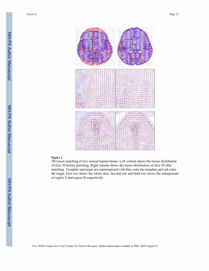
Figure 1.3D tensor matching of two normal human brains. Left column shows the tensor distributionof slice 30 before matching; Right column shows the tensor distribution of slice 30 aftermatching. Template and target are superimposed with blue color the template and red colorthe target. First row shows the whole slice. Second row and third row shows the enlargementof region A and region B respectively.

Cao et al. Page 15

Proc IEEE Comput Soc Conf Comput Vis Pattern Recognit. Author manuscript; available in PMC 2010 August 12.

NIH

-PA

Author M

anuscriptN

IH-P

A A

uthor Manuscript

NIH

-PA

Author M

anuscript

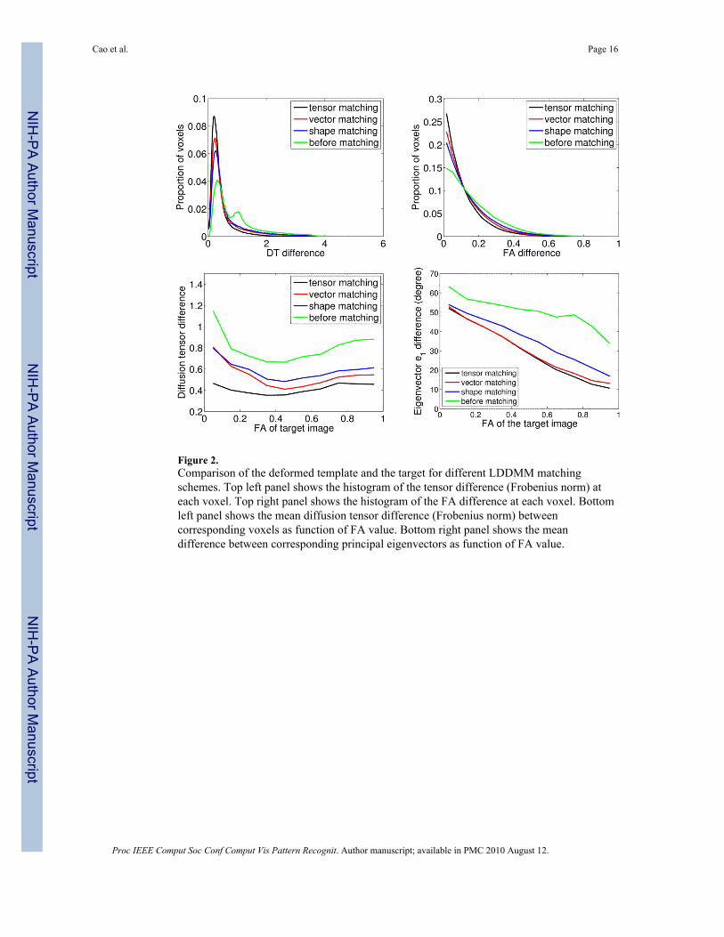
Figure 2.Comparison of the deformed template and the target for different LDDMM matchingschemes. Top left panel shows the histogram of the tensor difference (Frobenius norm) ateach voxel. Top right panel shows the histogram of the FA difference at each voxel. Bottomleft panel shows the mean diffusion tensor difference (Frobenius norm) betweencorresponding voxels as function of FA value. Bottom right panel shows the meandifference between corresponding principal eigenvectors as function of FA value.

Cao et al. Page 16

Proc IEEE Comput Soc Conf Comput Vis Pattern Recognit. Author manuscript; available in PMC 2010 August 12.

NIH

-PA

Author M

anuscriptN

IH-P

A A

uthor Manuscript

NIH

-PA

Author M

anuscript

Figure 3.Comparison of the deformations result from LDDMM vector matching and tensor matchingschemes. Top panel shows the FA weighted color-coded orientation map of the target.Second row shows the deformations from vector matching, third row shows the deformationfrom tensor matching. First column shows the the determinant of the Jacobian matrix..Second column shows the rotation part of the Jacobian matrix, the rotation angle in degree.Third column shows the normalized difference of the eigenvalues of the Jacobian matrix.Tensor matching scheme improves the matching quality in areas with low FA values.

Cao et al. Page 17

Proc IEEE Comput Soc Conf Comput Vis Pattern Recognit. Author manuscript; available in PMC 2010 August 12.

NIH

-PA

Author M

anuscriptN

IH-P

A A

uthor Manuscript

NIH

-PA

Author M

anuscript

Figure 4.Left column shows the histogram of 3 tensor eigenvalues for several normal human brainDT-MRI datasets, right column shows the histogram of 3 tensor eigenvalues for severalnormal canine heart DT-MRI datasets. Same color means the same dataset. This figureshows sometimes it necessary to normalize the eigenvalues of the tensors before matching.

Cao et al. Page 18

Proc IEEE Comput Soc Conf Comput Vis Pattern Recognit. Author manuscript; available in PMC 2010 August 12.

NIH

-PA

Author M

anuscriptN

IH-P

A A

uthor Manuscript

NIH

-PA

Author M

anuscript