Diffeomorphic Matching of Distributions: A New Approach for Unlabelled Point-Sets and Sub-Manifolds...

Diffeomorphic matching of distributions:A new approach for unlabelled point-sets and sub-manifolds matching

Joan Glaunes Alain Trouve Laurent Younes

LAGA CMLA CISUniversite Paris 13 ENS de Cachan Johns Hopkins University

Villetaneuse, FRANCE Cachan, FRANCE Baltimore, Md 21218

Abstract

In the paper, we study the problem of optimal matchingof two generalized functions (distributions) via a diffeomor-phic transformation of the ambient space. In the particu-lar case of discrete distributions (weighted sums of Diracmeasures), we provide a new algorithm to compare twoarbitrary unlabelled sets of points, and show that it be-haves properly in limit of continuous distributions on sub-manifolds. As a consequence, the algorithm may apply tovarious matching problems, such as curve or surface match-ing (via a sub-sampling), or mixings of landmark and curvedata. As the solution forbids high energy solutions, it is alsorobust towards addition of noise and the technique can beused for nonlinear projection of datasets. We present 2Dand 3D experiments.

1.. Introduction

Matching embedded geometric structures is of particu-lar importance in many computer vision tasks and medicalimaging problems. The setting generally includes two im-ages or volumes, within which points, curves or surfaceshave been extracted, and formulates the following prob-lems:

1. Detect suitable correspondences between the mani-folds extracted from the first image and those extractedfrom the second.

2. Interpolate these correspondences to obtain a densedisplacement field between the two images.

In most of the approaches developped for matching (like[3, 4, 14, 10, 1, 8, 13, 5]), the considered geometric struc-tures are points and both problems are solved separately:the second is addressed by elastic matching techniques cou-pled with spline interpolation, and the first one (point topoint correspondence) is most of the time solved by hand(labels being provided by experts), in the absence of a reli-able matching procedure. As an exception, [16] addresses

the problems simultaneously, with the paradigm that thebest correspondences should correspond to the smoothestdeformations, yielding an automated point matching proce-dure. To match higher dimensional structures (curves andsurfaces), the same approach is used, after discretizationand representation by a set of points.

However, curve and surface matching cannot be con-sidered as limit problems of point matching (through dis-cretization), because a given point in the discretized firstmanifold should be matched to some point of the secondmanifold, but not necessarily belonging to the set of pointsinto which this manifold has been discretized. Our argu-ment in this paper is that all these problems (surface, curveand unlabeled point matching) all are particular instances ofa more general class of problems, which is matching mea-sures onR2 orR3, and more generally distributions on thesesets (ie. generalized functions). For this purpose, we de-velop a theory based on the action of diffeomorphisms ondistributions (which we present here in the specific case ofmeasures), along the lines of Grenander’s deformable tem-plates theory ([12]), and in the large-deformation setting, asdeveloped in [17, 9, 15, 2, 11].

A significant contribution related to unlabeled pointmatching has been provided with the Robust Point Match-ing algorithm (RPM) [6] and further refinements with theJoint Clustering and Matching Algorithm (JCM) [7]. There,the approach essentially consists in estimating and match-ing two probability distributions, modeled as mixtures ofGaussians, with the assumptions that the second one is ob-tained from the first one by the action of an unknowndeformation field on its centers, and that the two unla-beled point sets are random samples of these distribu-tions. Such an approach, however, does not incorporatethe important constraint that the estimated deforma-tion is smooth and invertible. Moreover, the consistencyissue is not addressed, and very hard to assert: this corre-sponds to the limit behavior of the algorithm in the casewhen the centers of the mixtures of Gaussian are them-

selves obtained by discretizing two curves or surfaces,and the limit is taken with respect to the discretization ac-curacy. This is a fundamental issue, which essentiallydecides of the numerical reliability of the matching algo-rithm.

2.. Mathematical Setup

2.1.. Large deformation framework

This section provides the required component of the“large deformation framework” for diffeomorphic match-ing. In this setting, the starting object is a Hilbert spaceV ,with norm | |V , of smooth vector fields (at leastC1) de-fined on the background spaceRd. This space induces asub-groupGV of diffeomorphisms as follows: to any time-dependent vector fieldv : t → vt, is associated the flowequation

∂tφt = vt φt, φ0(x) = x , (1)

which has a unique solution starting atφ0 = id whent 7→ |vt|V is integrable and under suitable regularity con-ditions on the elements ofV ([9]). Then GV , defined byGV = φv

1 | |vt|V ∈ L1 , is a group, which can beequipped with a natural right-invariant geodesic distanced(φ, φ′) = inf

∫ 1

0|vt|V dt | φv

1 φ = φ′.

2.2.. Group action on measures

Consider the setMs of all signed measures (differenceof two finite positive measures) onRd. The groupGV actsonMs according to the action(φ, µ)→ φµ with

φµ(f) =∫

f φdµ (2)

for any bounded measurable functionf . In the case of a dis-crete measureµ =

∑i αiδxi (whereδx is the Dirac mass

at locationx), we haveφµ =∑

i αiδφ(xi). The problemof matching two signed measuresµ andν will be formu-lated as findingφ ∈ GV as close as possible to the identitymapping (for the distanced onGV ) such thatφµ is close toν, for some metric between measures, both constraints be-ing represented by penalty terms in a variational problem.To specify the metric which is used to compareφµ andν,we introduce a second Hilbert spaceI, with norm| |I , con-taining continuous, boundedfunctionsonRd, with the con-straint

|f |∞ ≤ c|f |I (3)

for a givenc. Let I∗ be the space of continuous linear formson I. Assumption (3) implies that integration with respectto signed measure, which is a continuous linear form onbounded continuous functions is also continuous for theHilbert structure onI, so thatMs can also be consideredas a subset ofI∗. The distance between two signed mea-suresµ andµ′ is now taken as|µ − µ′|I∗ , with the usualdefinition:|ν|I∗ = sup(

∫fdµ, f ∈ I, |f |I = 1).

This norm can be computed as follows. The Riesz rep-resentation theorem implies that, for ally ∈ Rd, thereexists an element,KIδy of I such that, for allf ∈ I,f(y) =

∫fdδy = 〈KIδy, f〉I . This implies that, for all

µ ∈Ms,∫f(y)dµ(y) =

∫〈KIδy, f〉Idµ(y) =

⟨ ∫KIδydµ(y), f

⟩I

In particular, denotingKIµ =∫

KIδydµ(y), and taking thesupremum of both sides over allf with |f |I = 1, we have

|µ|2I∗ = |KIµ|2I =∫

KIµ(x)dµ(x)

which finally yields, denotingkI(y, x) = (KIδy)(x)

|µ|2I∗ =∫

kI(x, y)dµ(x)dµ(y) (4)

If µ =∑

i ciδxi is a weighted sum of Dirac measures, thisyields

|µ|2I∗ =∑i,j

cicjkI(xi, xj)

which is particularly simple whenkI is given.

2.3.. Variational formulation

We define the optimal matching,φ between two signedmeasuresµ andν as a minimizer ofJµ,ν(φ) .= d(Id, φ)2 +|φµ−ν|2I∗/σ2

R, σ2R being a trade-off parameter. Introducing

the kinetic energy∫ 1

0|vt|2V dt, we get equivalently thatφ =

φv1 (cf (1)) wherev is a minimizer of

Jµ,ν(v) =∫ 1

0

|vt|2V dt +1

σ2R

|φv1µ− ν|2I∗ (5)

An attractive aspect of this variational formulation is itsability to handle point sets matching problems for whichµandν are two positive discrete measures and the limit prob-lem of matching continuous distributions supported by sub-manifolds.

2.4.. Existence and consistency results

In this subsection we state, without proofs, two impor-tant properties of this variational formulation. The first oneis an existence theorem, which is true under suitable regu-larity conditions onV .

Theorem 1 (Existence)For givenµ, ν inMs there existsa minimizing solutionv of (5).

The second one is the consistency property mentionned inthe introduction, still valid under suitable regularity condi-tions onV .

Theorem 2 (Consistency)Let µ andν be twoprobabilitydistributions onRd and letx1, · · · , xm andy1, · · · , yn beiid samples drawn from distributionsµ and ν. Let µm =1m

∑i δxi

and νn = 1n

∑j δyj

be the associated empiri-

cal measures. Then ifφ(m,n) is a minimizer ofJµm,νn, al-

most surely,φ(m,n) tends uniformly (up to the extraction ofa subsequence) toφ, minimizer ofJµ,ν , whenm,n→∞.

3.. Derivation of the algorithm

3.1.. Gradient computation for general measures

Our estimation of the optimal matching between two dis-tributionsµ andν is based on the implementation of a gra-dient algorithm for

J(v) =∫ 1

0

|vt|2V dt +1

σ2R

|φv1µ− ν|2I∗

in L2([0, 1], V ), the Hilbert space of time-dependent ele-ments ofV with square integrable norms.

We compute the variations ofJ with respect to a varia-tion vh = v + hv. For a given quantityA, we denoteA thevariation ofA with respect toh, i.e. the derivative ofAh ath = 0.

Since the variation of the first term is straightforward, wefocus on the second termE = |φv

1µ− ν|2I∗ . We have

E = 2〈φv1µ, φv

1µ− ν〉I∗

Let KI : I∗ → I be the canonical isometry betweenIand its dual spaceI∗ generated by the Riesz representa-tion theorem i.e. for anyν ∈ I∗ and g ∈ I, ν(g) =〈KIν, g〉I = 〈ν,K−1

I g〉I∗ . This operator has already beenintroduced, as applied to measures, in section 2.1. Letf1 =KI(φv

1µ− ν) ∈ I. Sinceφv1µ ∈ I∗, we can write

E = 2φv1µ(f1) = µ(f1 φv

1 ) = µ(dφv1f1.φv

1 ).

Now, denotingφvst = φv

t (φvs )−1, the variation of the de-

formation mapφv1 satisfies [2],

φv1 =

∫ 1

0

dφvtφv

t1.vt φvt dt.

Therefore,

dφv1f1.φv

1 =∫ 1

0

(d(f1 φvt1).vt) φv

t dt,

and thus

E =∫ 1

0

φvt µ(d(f1 φv

t1).vt)dt

=∫ 1

0

(∫Rd

dx(f1 φvt1).vt(x)d(φv

t µ))

dt

=∫ 1

0

(∫Rd

〈∇x(f1 φvt1), vt(x)〉d(φv

t µ))

dt.

The linear form

φvt µ∇(f1 φv

t1) : u 7→∫

Rd

〈∇x(f1 φvt1),ut(x)〉d(φv

t µ)

is continuous onV and therefore belongs toV ∗. Introduc-ing, as above, the operatorKV : V ∗ → V inducing thecanonical isometry, we find

E =∫ 1

0

〈KV (φvt µ∇(f1 φv

t1)), vt〉V dt,

and the gradient ofJ in L2([0, 1], V ) writes

(∇J)t(x) = 2vt(x)+2

σ2R

KV (φvt µ∇(KI(φv

1µ−ν)φvt1)).

(6)

3.2.. Application to Dirac measures

When measuresµ and ν are weighted sums of Diracmeasures,µ =

∑mi=1 aiδxi

andν =∑n

i=1 biδyi, the for-

mula for J and its gradient can be rewritten to provide anexplicit formulation of the variational problem. We use thenotationxi(t) = φv

t (xi) and

φv1µ− ν =

m∑i=1

aiδxi(t) −n∑

i=1

biδyi=

nz∑i=1

ciδzi.

First, the error term ofJ writes

E = |φv1µ− ν|2I∗ =

nz∑i,j=1

cicjkI(zi, zj).

Now we use the following remark : when trajectoriesxi(t) are fixed, the vector fields of lowest energy take theform

vt(x) =m∑

i=1

kV (xi(t), x)αi(t),

where kV (x, y) is the kernel operator correspond-ing to space V , which satisfies β∗kV (x, y)α =〈kV (x, ·)α, kV (y, ·)β〉V . This is a general fact for land-mark matching methods [13, 5].

Thus, the variables of our minimization problem becomethe vectorsαi(t) and the functionalJ rewrites

J =∫ 1

0

m∑i,j=1

αj(t)∗kV (xi(t), xj(t))αi(t)

+1

σ2R

nz∑i,j=1

cicjkI(zi, zj)

dt.

Next we compute the explicit formulation of the gradientto be implemented in the matching code. We have

f1(x) = KI(φv1µ− ν)(x) =

nz∑i=1

cikI(zi, x),

f1 φvt1(x) =

nz∑i=1

cikI(zi, φvt1(x)),

∇(f1 φvt1)(x) =

nz∑i=1

ci(dxφvt1)

∗.∇2kI(zi, φvt1(x)).

Moreover,φvt µ =

∑mi=1 aiδxi(t), so if we denote byδα

x theelement ofV ∗ such thatδα

x (u) = 〈u(x), α〉, we have

φvt µ∇(f1 φv

t1) =m∑

j=1

ajδβj(t)

xj(t),

with βj(t) = (dxj(t)φvt1)

∗.βj(1) and

βj(1) =nz∑i=1

ci∇2kI(zi, φv1 (xj)). (7)

The gradient expression is

(∇J)t(x) = 2m∑

j=1

kV (xj(t), x)(αj(t) + βj(t)/σ2R).

The quantityβj(t) can be computed by numerical integra-tion, since we have :

dxj(t)φvt1 = dxj

φv1 .(dxj

φvt )−1,

∂t(dxjφv

t )−1 = −(dxjφv

t )−1.dxj(t)vt,

∂tdxj(t)φvt1 = −dxj(t)φ

vt1.dxj(t)vt,

and eventually,

∂tβj(t) = (∂tdxj(t)φvt1)

∗.βj(1) = −(dxj(t)vt)∗.βj(t).(8)

Now sincevt =∑m

k=1 kV (xk(t), ·)αk(t), we have

dxj(t)vt =nx∑

k=1

∂2kV (xk(t), xj(t))αk(t).

4. Experiments

5. Experiments

This section presents simulations processed on syntheticexamples with a MATLAB implementation of a gradientdescent on the functionalJ , as given by formula 7. We haveused kernelskV andkI defined onΩ = R2 and such that

kV (x, y) = fV

(|x− y|2

σ2V

)Id

kI(x, y) = fI

(|x− y|2

σ2I

),

i.e. kV and kI are isotropic, translation and rotation in-variant. For functionsfV and fI wa have triedfV (u) =fI(u) = exp(−u) (gaussian kernels) andfV (u) = fI(u) =

11+u . This second choice gives the best results and has beenselected for the simulations.

The main steps of the gradient descent algorithm are

• InitialisationSet initial trajectoriesxi(t) = xi andαi(t) = 0

• Iteration loop :(x, α)→ (x, α).

– Computeβj(1) with formula 7.

– Computeβj(t) by integrating equation 8.

– Setαi(t) ← αi(t) − λ(2αi(t) + βi(t)) whereλis the gradient step.

– Compute new trajectoriesxi(t) by integrating

∂txi(t) =m∑

i=1

kV (xj(t), xi(t))αj(t).

– Compute new vectorsαi(t) by inverting the lin-ear systems

∂txi(t) =m∑

i=1

kV (xj(t), xi(t))αj(t).

The two last steps are actually needed to ensure thatduring minimization, trajectoriesxi(t) are kept equal toφv

t (xi), wherev is computed fromαi(t).

0 0.2 0.4 0.6 0.8 10

0.1

0.2

0.3

0.4

0.5

0.6

0.7

0.8

0.9

1sigmaV=0.5, sigmaI=0.1, sigma=0.01, 0 itérations

−0.2 0 0.2 0.4 0.6 0.8 1 1.2

0.1

0.2

0.3

0.4

0.5

0.6

0.7

0.8

0.9

1

1.1

sigmaV=0.5, sigmaI=0.1, sigma=0.01, 782 itérations

Figure 1. Matching with two pairs curves (seetext for details).

Figure 1 shows the result of matching two pairs ofsmapled curves. Initial landmark points (lowest and right-most curves) are drawn as diamonds and targets as stars.Note that these are the only information given to the algo-rithm for the minimization process. In particular, the algo-rithm does not ”know” that there are two curves. On theright frame (final state) are drawn the target curve and the

deformation of the whole initial curve which superimposealmost exactly.

Figure 1 shows the result of a matching process betweentwo pairs of curves given by their sampling. Initial land-mark points are drawn as diamonds and targets as stars.Note that these are the only information given to the algo-rithm for the minimization process. In particular, the algo-rithm do not ”know” that there are two curves. On the rightframe (final state) are drawn the target curve and the defor-mation of the whole initial curve.

0 0.2 0.4 0.6 0.8 10

0.1

0.2

0.3

0.4

0.5

0.6

0.7

0.8

0.9

1sigmaV=0.5, sigmaI=0.1, sigma=1e−005, 0 itérations

0 0.2 0.4 0.6 0.8 1

0.1

0.2

0.3

0.4

0.5

0.6

0.7

0.8

0.9

1

sigmaV=0.5, sigmaI=0.1, sigma=0.001, 84 itérations

Figure 2. Experiment with one curve and twolandmarks (see text for details).

Experiment 2 illustrates the possibility to perform amatching with both of landmark and curve data. For thesimulation we have assigned a weight of1/3 for each ofthe 2 landmarksand the curve, which means each of the 12sample points of the curve has weight1/36; thus equal im-portance is given to the three items.

Experiment 3 explores the robustness of the algorithmagainst the presence of outliers. It shows how the deforma-tion varies when more and more random points are addedboth to the initial and target datasets. The conclusion is that,while the global deformation may be affected by the noise,its effect on the initial curve remains essentially constant.

Next (figures 3,4,5,6) we have processed a series of ex-periments of matching a circle to a deformed closed curve.The only curve which is drawn is the image of the initial cir-cle under the current deformation map (The initial circle islocates on the lower-left part of the grid).

In figure 4 we sample the curves at various rates and pro-cess the algorithm with the same parameters. When sam-pling rates are equal, the algorithm matches exactly pairs oflandmarks. The interesting case comes with different sam-pling rates : in this case the deformed data fits along thetarget curve without matching specifically any of its land-marks. This illustrates the consistency of the algorithm, asexplained in the section 2.4.

In figure 5 a gaussian noise is added to the positionsof the target landmarks, with increasing variance. The de-formed curve remains remarkably stable, finding an aver-

0 0.2 0.4 0.6 0.8 1

0.1

0.2

0.3

0.4

0.5

0.6

0.7

0.8

0.9

1sigmaV=0.5, sigmaI=0.1, sigmaR=0.001, 300 itérations

0 0.2 0.4 0.6 0.8 1

0.1

0.2

0.3

0.4

0.5

0.6

0.7

0.8

0.9

1

sigmaV=0.5, sigmaI=0.1, sigmaR=0.001, 210 itérations

0 0.2 0.4 0.6 0.8 1

0.1

0.2

0.3

0.4

0.5

0.6

0.7

0.8

0.9

1


0 0.2 0.4 0.6 0.8 1 1.20

0.1

0.2

0.3

0.4

0.5

0.6

0.7

0.8

0.9

1


Figure 3. Robustness against outliers (0, 20,40 and 60 outlier points added)

0 0.5 1 1.5 2

0

0.2

0.4

0.6

0.8

1

1.2

1.4

1.6


0 0.5 1 1.5 2

0

0.2

0.4

0.6

0.8

1

1.2

1.4

1.6


sampling rates 10 and 10 sampling rates 10 and 7

0 0.5 1 1.5 2

0

0.2

0.4

0.6

0.8

1

1.2

1.4

1.6


0 0.5 1 1.5 2

0

0.2

0.4

0.6

0.8

1

1.2

1.4

1.6


sampling rates 10 and 2 sampling rates 2 and 2

Figure 4. Comparing different sampling rates.

0 0.5 1 1.5 2

0

0.2

0.4

0.6

0.8

1

1.2

1.4

1.6


0 0.5 1 1.5 2

0

0.2

0.4

0.6

0.8

1

1.2

1.4

1.6


−0.5 0 0.5 1 1.5 2

−0.2

0

0.2

0.4

0.6

0.8

1

1.2

1.4

1.6


−0.5 0 0.5 1 1.5 2

−0.2

0

0.2

0.4

0.6

0.8

1

1.2

1.4

1.6

1.8


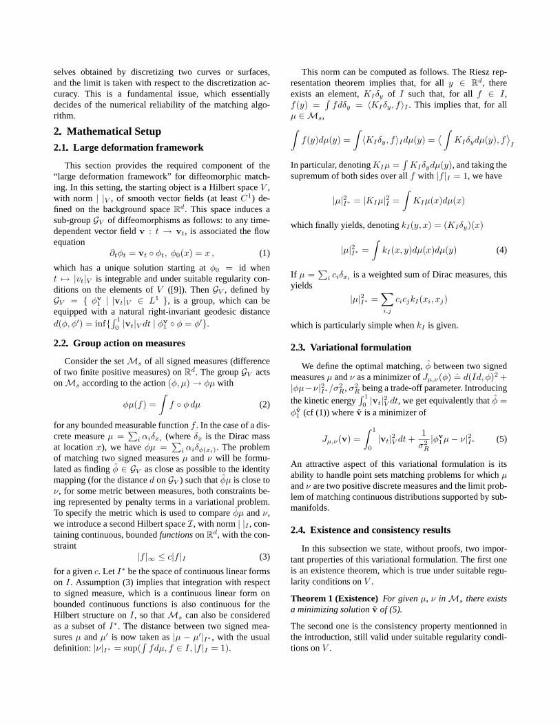
Figure 5. Analyzing the effect of noisy data(variances of noise are 0, 0.01, 0.03, and 0.1)

age position within the target points, even for significantlylarge noise.

In figure 6 we vary the parametersσV andσI and pro-cess a noisy data sample (the third one in figure 5). Whenthese parameters decrease, the deformation map becomesmore sensitive to local variations of the data.

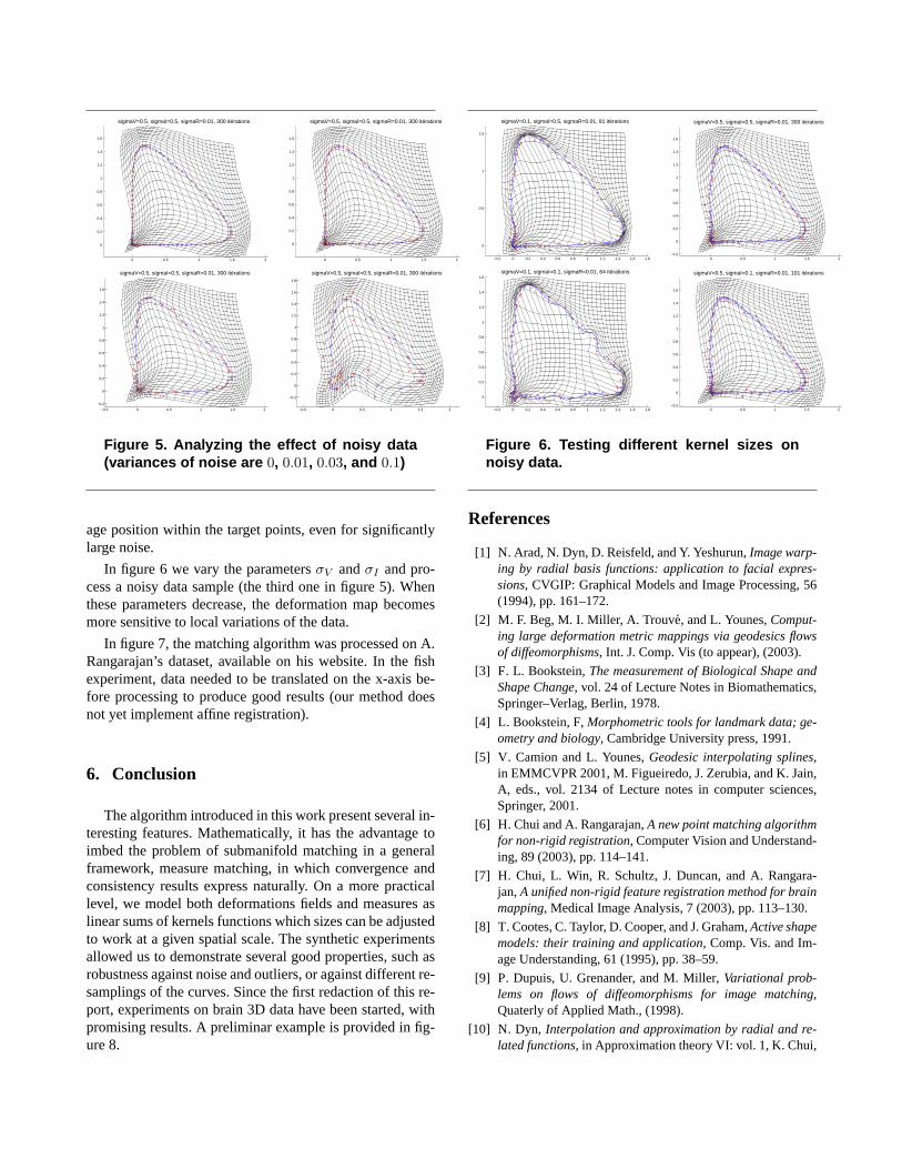
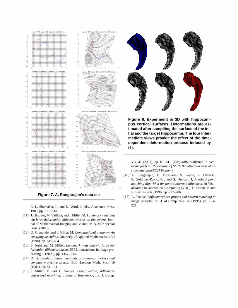
In figure 7, the matching algorithm was processed on A.Rangarajan’s dataset, available on his website. In the fishexperiment, data needed to be translated on the x-axis be-fore processing to produce good results (our method doesnot yet implement affine registration).

6. Conclusion

The algorithm introduced in this work present several in-teresting features. Mathematically, it has the advantage toimbed the problem of submanifold matching in a generalframework, measure matching, in which convergence andconsistency results express naturally. On a more practicallevel, we model both deformations fields and measures aslinear sums of kernels functions which sizes can be adjustedto work at a given spatial scale. The synthetic experimentsallowed us to demonstrate several good properties, such asrobustness against noise and outliers, or against different re-samplings of the curves. Since the first redaction of this re-port, experiments on brain 3D data have been started, withpromising results. A preliminar example is provided in fig-ure 8.

−0.2 0 0.2 0.4 0.6 0.8 1 1.2 1.4 1.6 1.8

0

0.5

1

1.5


0 0.5 1 1.5 2−0.2

0

0.2

0.4

0.6

0.8

1

1.2

1.4

1.6


−0.2 0 0.2 0.4 0.6 0.8 1 1.2 1.4 1.6 1.8

0

0.2

0.4

0.6

0.8

1

1.2

1.4

1.6sigmaV=0.1, sigmaI=0.1, sigmaR=0.01, 64 itérations

0 0.5 1 1.5 2−0.2

0

0.2

0.4

0.6

0.8

1

1.2

1.4

1.6


Figure 6. Testing different kernel sizes onnoisy data.

References

[1] N. Arad, N. Dyn, D. Reisfeld, and Y. Yeshurun,Image warp-ing by radial basis functions: application to facial expres-sions, CVGIP: Graphical Models and Image Processing, 56(1994), pp. 161–172.

[2] M. F. Beg, M. I. Miller, A. Trouve, and L. Younes,Comput-ing large deformation metric mappings via geodesics flowsof diffeomorphisms, Int. J. Comp. Vis (to appear), (2003).

[3] F. L. Bookstein,The measurement of Biological Shape andShape Change, vol. 24 of Lecture Notes in Biomathematics,Springer–Verlag, Berlin, 1978.

[4] L. Bookstein, F,Morphometric tools for landmark data; ge-ometry and biology, Cambridge University press, 1991.

[5] V. Camion and L. Younes,Geodesic interpolating splines,in EMMCVPR 2001, M. Figueiredo, J. Zerubia, and K. Jain,A, eds., vol. 2134 of Lecture notes in computer sciences,Springer, 2001.

[6] H. Chui and A. Rangarajan,A new point matching algorithmfor non-rigid registration, Computer Vision and Understand-ing, 89 (2003), pp. 114–141.

[7] H. Chui, L. Win, R. Schultz, J. Duncan, and A. Rangara-jan,A unified non-rigid feature registration method for brainmapping, Medical Image Analysis, 7 (2003), pp. 113–130.

[8] T. Cootes, C. Taylor, D. Cooper, and J. Graham,Active shapemodels: their training and application, Comp. Vis. and Im-age Understanding, 61 (1995), pp. 38–59.

[9] P. Dupuis, U. Grenander, and M. Miller,Variational prob-lems on flows of diffeomorphisms for image matching,Quaterly of Applied Math., (1998).

[10] N. Dyn, Interpolation and approximation by radial and re-lated functions, in Approximation theory VI: vol. 1, K. Chui,

−0.2 0 0.2 0.4 0.6 0.8 1 1.2

−0.6

−0.4

−0.2

0

0.2

0.4

0.6


−0.4 −0.2 0 0.2 0.4 0.6 0.8 1 1.2

−0.6

−0.4

−0.2

0

0.2

0.4

0.6

0.8


0.1 0.2 0.3 0.4 0.5 0.6 0.7 0.80

0.1

0.2

0.3

0.4

0.5

0.6


0.1 0.2 0.3 0.4 0.5 0.6 0.7 0.8 0.9

−0.1

0

0.1

0.2

0.3

0.4

0.5


−0.2 −0.1 0 0.1 0.2 0.3 0.4 0.5 0.6

0.3

0.4

0.5

0.6

0.7

0.8

0.9

1sigmaV=0.5, sigmaI=0.1, sigmaR=0.01, 0 itérations

−0.1 0 0.1 0.2 0.3 0.4 0.5 0.6

0.3

0.4

0.5

0.6

0.7

0.8

0.9


0.2 0.3 0.4 0.5 0.6 0.7 0.8 0.9 1 1.1 1.2

0.1

0.2

0.3

0.4

0.5

0.6

0.7

0.8

0.9


0.2 0.4 0.6 0.8 1 1.2 1.4

0

0.1

0.2

0.3

0.4

0.5

0.6

0.7

0.8

0.9


Figure 7. A. Rangarajan’s data set

C, L. Shumaker, L, and D. Ward, J, eds., Academic Press,1989, pp. 211–234.

[11] J. Glaunes, M. Vaillant, and I. Miller, M,Landmark matchingvia large deformation diffeomorphisms on the sphere, Jour-nal of Mathematical Imaging and Vision, MIA 2002 specialissue, (2003).

[12] U. Grenander and I. Miller, M,Computational anatomy: Anemerging discipline, Quarterly of Applied Mathematics, LVI(1998), pp. 617–694.

[13] S. Joshi and M. Miller,Landmark matching via large de-formation diffeomorphisms, IEEE transactions in image pro-cessing, 9 (2000), pp. 1357–1370.

[14] D. G. Kendall,Shape manifolds, procrustean metrics andcomplex projective spaces, Bull. London Math. Soc., 16(1984), pp. 81–121.

[15] I. Miller, M and L. Younes, Group action, diffeomor-phism and matching: a general framework, Int. J. Comp.

Figure 8. Experiment in 3D with hippocam-pus cortical surfaces. Deformations are es-timated after sampliing the surface of the ini-tial and the target Hippocampi. The four inter-mediate views provide the effect of the time-dependent deformation process induced by(1).

Vis, 41 (2001), pp. 61–84. (Originally published in elec-tronic form in: Proceeding of SCTV 99, http://www.cis.ohio-state.edu/ szhu/SCTV99.html).

[16] A. Rangarajan, E. Mjolsness, S. Pappu, L. Davachi,S. Goldman-Rakic, P, , and S. Duncan, J,A robust pointmatching algorithm for autoradiograph alignment, in Visu-alization in Biomedical Computing (VBC), H. Hohne, K andR. Kikinis, eds., 1996, pp. 277–286.

[17] A. Trouve,Diffeomorphism groups and pattern matching inimage analysis, Int. J. of Comp. Vis., 28 (1998), pp. 213–221.

Diffeomorphic Matching of Distributions: A New Approach for Unlabelled Point-Sets and Sub-Manifolds...

Documents

Transcript of Diffeomorphic Matching of Distributions: A New Approach for Unlabelled Point-Sets and Sub-Manifolds...