Parametric manifolds. I. Extrinsic approach
16
Parametric manifolds. I. Extrinsic approach Stuart Boersmaa) and Tevian Drayb) Department of Mathematics, Oregon State Universi& Corvallis, Oregon 97331 (Received 18 July 1994; accepted for publication 24 August 1994) A parametric manifold can be viewed as the manifold of orbits of a (regular) foliation of a manifold by means of a family of curves. If the foliation is hypersur- face orthogonal, the parametric manifold is equivalent to the one-parameter family of hypersurfaces orthogonal to the curves, each of which inherits a metric and connection from the original manifold via orthogonal projections; this is the well- known Gauss-Codazzi formalism. This formalism is generalized to the case where the foliation is not hypersurface orthogonal. Crucial to this generalization is the notion of dejkiency, which measures the failure of the orthogonal tangent spaces to be surface forming, and which behaves very much like torsion. Some applications to initial value problems in general relativity will be briefly discussed. 0 1995 American Institute of Physics. I. INTRODUCTION Associated with a foliation of space-time by spacelike hypersurfaces is the dual foliation by timelike curves orthogonal to the hypersurfaces, i.e., the trajectories of observers whose instanta- neous rest spaces consist precisely of the given hypersurfaces. But how does one describe physics as seen by observers whose trajectories are not hypersurface orthogonal? It is the goal of this article to describe one possible framework for answering such questions. The decomposition of various fields on a manifold into data on a hypersurface is not merely of interest for space-times. Given a (nondegenerate) metric of any signature on a manifold L%, the Gauss-Codazzi equations show how to project the geometry of & orthogonally onto a hypersurface 2. This article generalizes the Gauss-Codazzi equations which describe the geom- etry orthogonal to a given family of curves to include the case when these curves fail to be hypersurface orthogonal. The term parametric manifold has been recently coined by Perjis’ in this setting. He traces some of the geometric ideas back to Zel’manov;’ similar ideas can also be found in some work of Einstein and Bergmann on Kaluza-Klein theories. However, none of these authors describe the parametric theory in modem mathematical language, as tensors are given in terms of their com- ponents in a coordinate basis and their abstract properties are not clear. In particular, defining torsion in this setting, and especially distinguishing it from the new concept of dejciency, is hard to do without a basis-free approach. This article presents one way of unifying these earlier ideas into a rigorous mathematical framework. We start by reviewing some basic properties of connections in Sec. II, followed by a descrip- tion of the usual Gauss-Codazzi formalism in Sec. III. We have deliberately presented some fairly standard material in considerable detail so that the comparison with the generalized Gauss- Codazzi framework, described in Sec. IV, will be clear. In Sec. V, we express our results in a coordinate basis so that it can be more easily compared to earlier work. In Sec. VI we then show that our framework does not, in fact, completely reproduce the earlier results cited above, and we further show how this can be remedied. Finally, in Sec. VII, we discuss our results. ‘)Present address: Division of Mathematics and Computer Science, Alfred University, Alfred, NY 14802; E-mail: [email protected] b)E-mail: [email protected] 1378 J. Math. Phys. 36 (3), March 1995 0022-2488/95/36(3)/1378/16/$6.00 0 1995 American Institute of Physics Downloaded 19 Aug 2013 to 128.193.163.10. This article is copyrighted as indicated in the abstract. Reuse of AIP content is subject to the terms at: http://jmp.aip.org/about/rights_and_permissions
-
Upload
khangminh22 -
Category
Documents
-
view
0 -
download
0
Transcript of Parametric manifolds. I. Extrinsic approach
Parametric manifolds. I. Extrinsic approach Stuart Boersmaa) and Tevian Drayb) Department of Mathematics, Oregon State Universi& Corvallis, Oregon 97331
(Received 18 July 1994; accepted for publication 24 August 1994)
A parametric manifold can be viewed as the manifold of orbits of a (regular) foliation of a manifold by means of a family of curves. If the foliation is hypersur- face orthogonal, the parametric manifold is equivalent to the one-parameter family of hypersurfaces orthogonal to the curves, each of which inherits a metric and connection from the original manifold via orthogonal projections; this is the well- known Gauss-Codazzi formalism. This formalism is generalized to the case where the foliation is not hypersurface orthogonal. Crucial to this generalization is the notion of dejkiency, which measures the failure of the orthogonal tangent spaces to be surface forming, and which behaves very much like torsion. Some applications to initial value problems in general relativity will be briefly discussed. 0 1995 American Institute of Physics.
I. INTRODUCTION
Associated with a foliation of space-time by spacelike hypersurfaces is the dual foliation by timelike curves orthogonal to the hypersurfaces, i.e., the trajectories of observers whose instanta- neous rest spaces consist precisely of the given hypersurfaces. But how does one describe physics as seen by observers whose trajectories are not hypersurface orthogonal? It is the goal of this article to describe one possible framework for answering such questions.
The decomposition of various fields on a manifold into data on a hypersurface is not merely of interest for space-times. Given a (nondegenerate) metric of any signature on a manifold L%, the Gauss-Codazzi equations show how to project the geometry of & orthogonally onto a hypersurface 2. This article generalizes the Gauss-Codazzi equations which describe the geom- etry orthogonal to a given family of curves to include the case when these curves fail to be hypersurface orthogonal.
The term parametric manifold has been recently coined by Perjis’ in this setting. He traces some of the geometric ideas back to Zel’manov;’ similar ideas can also be found in some work of Einstein and Bergmann on Kaluza-Klein theories. However, none of these authors describe the parametric theory in modem mathematical language, as tensors are given in terms of their com- ponents in a coordinate basis and their abstract properties are not clear. In particular, defining torsion in this setting, and especially distinguishing it from the new concept of dejciency, is hard to do without a basis-free approach. This article presents one way of unifying these earlier ideas into a rigorous mathematical framework.
We start by reviewing some basic properties of connections in Sec. II, followed by a descrip- tion of the usual Gauss-Codazzi formalism in Sec. III. We have deliberately presented some fairly standard material in considerable detail so that the comparison with the generalized Gauss- Codazzi framework, described in Sec. IV, will be clear. In Sec. V, we express our results in a coordinate basis so that it can be more easily compared to earlier work. In Sec. VI we then show that our framework does not, in fact, completely reproduce the earlier results cited above, and we further show how this can be remedied. Finally, in Sec. VII, we discuss our results.
‘)Present address: Division of Mathematics and Computer Science, Alfred University, Alfred, NY 14802; E-mail: [email protected]
b)E-mail: [email protected]
1378 J. Math. Phys. 36 (3), March 1995 0022-2488/95/36(3)/1378/16/$6.00
0 1995 American Institute of Physics
Downloaded 19 Aug 2013 to 128.193.163.10. This article is copyrighted as indicated in the abstract. Reuse of AIP content is subject to the terms at: http://jmp.aip.org/about/rights_and_permissions
S. Boersma and T. Dray: Parametric manifolds. I. Extrinsic approach 1379
II. BACKGROUND
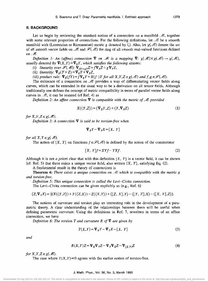
Let us begin by reviewing the standard notion of a connection on a manifold &%;, together with some relevant properties of connections. For the following definitions, let ,& be a smooth manifold with (Lorentzian or Riemannian) metric g denoted by (,). Also, let ,y(.&?S) denote the set of all smooth vector fields on .k% and .T(./%) th e ring of all smooth real-valued functions defined on . f&.
Definition 1: An (afine) connection V on ~8% is a mapping V: x(.&)X,y(.&) + &&‘), usually denoted by V(X, Y) =V,Y, which satisfies the following axioms:
(i) linearity over.F(.B): Vf,+,,Z=fVxZ+gVyZ, (ii) linearity: V,( Y +Z) =V,Y +V,Z, (iii) product rule: VxcfY) = f V,Y + Xcf ) Y f or all X,Y,ZEX(&) and f,g EF(.&%). The existence of a connection on ~85 provides a way of differentiating vector fields along
curves, which can be extended in the usual way to be a derivation on all tensor fields. Although traditionally one defines the concept of metric compatibility in terms of parallel vector fields along curves in . z%, it can be restated (cf Ref. 4) as
Definition 2: An afjine connection V is compatible with the metric of .&S provided
X((Y,Z))=(VxY,Z)+(Y,VxZ) (1) for X,Y,ZEx(&).
Definition 3: A connection V is said to be torsion-free when
V,Y-VyX=[X, Yl
for all X, Y EX(.J%). The action of [X, Y] on functions f&Q&%) is defined by the action of the commutator
[X, Y-jf=XYf - YXf. (2)
Although it is not a priori clear that with this definition [X, Y] is a vector field, it can be shown (cf. Ref. 5) that there exists a unique vector field, also written [X, Y], satisfying Eq. (2).
A fundamental result in the theory of connections is Theorem 4: There exists a unique connection on .& which is compatible with the metric g
and torsion-free. Definition 5: This unique connection is called the Levi-Civita connection. The Levi-Civita connection can be given explicitly as (e.g., Ref. 6)
(z~v,x)=~(x((y~z))+y((~,x))-z((x,Y))+([z, X],Y)-([Y, Z&X)-([X, Y],Z)).
The notions of curvature and torsion play an interesting role in the development of a para- metric theory. A clear understanding of the relationships between them will be useful when defining parametric curvature. Using the definitions in Ref. 7, rewritten in terms of an affine connection, we have
Definition 6: The torsion T and curvature R of V are given by
and
T(X,Y)=VxY-VyX-[X, Y] (3)
(4)
for X,Y,ZE&&). The case where T(X, Y) =O agrees with the earlier notion of torsion-free.
J. Math. Phys., Vol. 36, No. 3, March 1995
Downloaded 19 Aug 2013 to 128.193.163.10. This article is copyrighted as indicated in the abstract. Reuse of AIP content is subject to the terms at: http://jmp.aip.org/about/rights_and_permissions

1380 S. Boersma and T. Dray: Parametric manifolds. 1. Extrinsic approach
Consider the components of T and R in some patch with coordinates {x”), so that the coor- dinate vector fields {aJ form a (local) basis of x(.&). Defining the Christoffel symbols I& by Vaady = Q.3, we have
A torsion-free connection is thus sometimes referred to as a symmetric connection. While it is trivially true that mixed partial derivatives commute, the torsion tensor may be thought of as measuring the failure of mixed covariant derivatives to commute. As we see from above
where we have used the fact that VaJ = aJ = dfldxa. For curvature
As is often done, Rvspa may be expressed in terms of the Christoffel symbols YP,
(5)
It is worth noting that in the definition (4) of R, as well as in the formula (5) for the components Rpy+, there is no explicit mention of the torsion. The case is different when using the abstract index notation (see Ref. S), which closely parallels component notation in a coordinate basis.
In the abstract index notation, the vector field V,Y is represented by XaV,Yb. In a coordinate basis (with coordinates {x”)), Xn is the vector field X”a,. Furthermore, in this notation V,Zb = a,Zb + I’boZc would represent the tensor with components
B z + rQ7.
In the absence of torsion, one often defines the action of the Riemann curvature tensor by
R” cbaZn= cvavb- vbva)zc *
However, in terms of the Christoffel symbols rbca
Rewriting Eq. (6) yields the correct abstract index expression for the curvature tensor in the presence of torsion
Rnc&,= (v,vb- vbv,- Tm,bvm)zc. (7)
Thus, there is quite a difference between the treatment of torsion in the two notational schemes. While the first definition of curvature [Eq. (4)] proved to be valid with or without
J. Math. Phys., Vol. 36, No. 3, March 1995
Downloaded 19 Aug 2013 to 128.193.163.10. This article is copyrighted as indicated in the abstract. Reuse of AIP content is subject to the terms at: http://jmp.aip.org/about/rights_and_permissions
S. Boersma and T. Dray: Parametric manifolds. I. Extrinsic approach 1381
torsion, if one adopts the abstract index notation to describe a theory involving torsion, one must also redefine the curvature tensor to take this into account. While the abstract index notation is usually used to describe torsion-free theories (e.g., general relativity), we will see that the presence of “deficiency” in a parametric theory of space-time has analogous consequences.
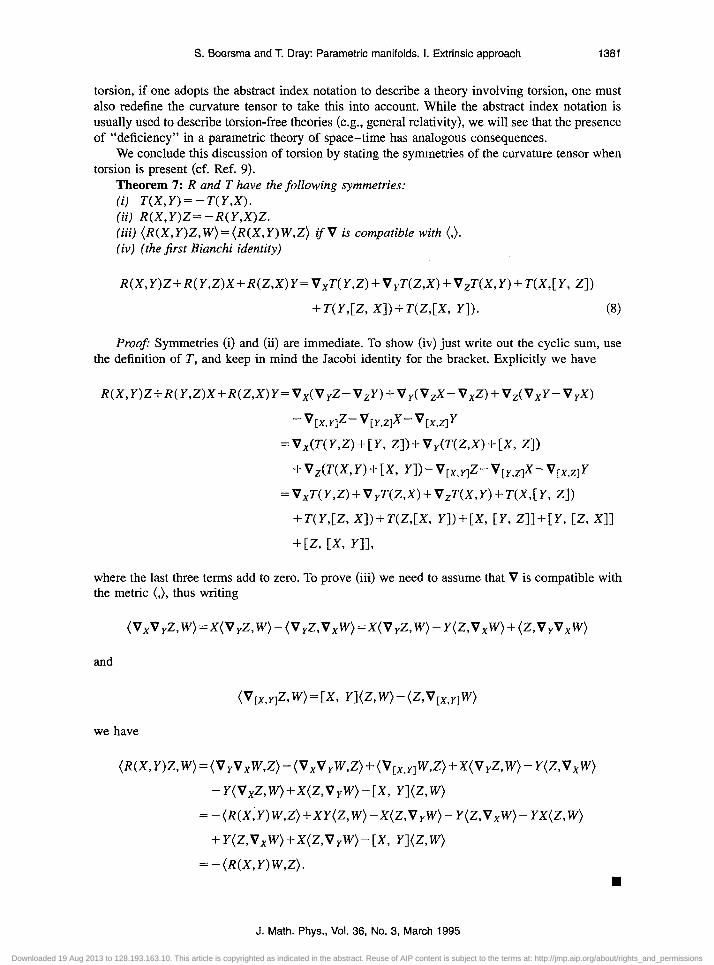
We conclude this discussion of torsion by stating the symmetries of the curvature tensor when torsion is present (cf. Ref. 9).
Theorem 7: R and T have the following symmetries: (i) T(X, Y) = - T( Y,X). (ii) R(X, Y)Z= - R( Y,X)Z. (iii) (R(X,Y)Z,W)=(R(X,Y)W,Z) ifV is compatible with (,). (iv) (the first Bianchi identity)
R(X,Y)Z+R(Y,Z)X+R(Z,X)Y=VxT(Y,Z)+VyT(Z,X)+V,T(X,Y)+T(X,[Y, Z])
+ T(Y,[Z, Xl> + TCUX, Yl>. (8)
Proof Symmetries (i) and (ii) are immediate. To show (iv) just write out the cyclic sum, use the definition of T, and keep in mind the Jacobi identity for the bracket. Explicitly we have
R(X,Y)Z+R(Y,Z)X+R(Z,X)Y=Vx(VyZ-VZY)+VY(VZX-VXZ)+VZ(VXY-VYX)
-~[~.Yl~-~~Y,zl~-~[x,zl~
= V,(T( Y,Z> + [Y, Zl)+ V y(T(Z,X) + LX, Zl)
+ Vz(T(X, Y) + [Xv Yl)- V[x,ylZ- V[,,$- V[x,z]Y =V,T(Y,Z)+V,T(Z,X)+V,T(X,Y)+T(X,[Y, Z])
+T(Y,[Z Xl)+WXX Yl)+[X, [Y, Zll+[Y, [Z, X +[z [XT Yll9
II
where the last three terms add to zero. To prove (iii) we need to assume that V is compatible with the metric (,), thus writing
and
we have
(R(X,Y)Z,W)=(Vy~xW,Z)-(~x~yW,Z)+(~~x,~~W,Z)+X(~~Z,W)-YY(Z~~xW)
-Y(v~z,w)+x(z,vYw>-cx, Yl(Z,W) =-(R(X;Y)W,Z)+XY(Z,W)-X(Z,VyW)-Y(Z,V,W)-YX(Z,W)
+Y(z,v~w)+x(z,vyw)-[X, Yl(ZW) =-(R(X,Y)W,Z).
H
J. Math. Phys., Vol. 36, No. 3, March 1995
Downloaded 19 Aug 2013 to 128.193.163.10. This article is copyrighted as indicated in the abstract. Reuse of AIP content is subject to the terms at: http://jmp.aip.org/about/rights_and_permissions
1382 S. Boersma and T. Dray: Parametric manifolds. 1. Extrinsic approach
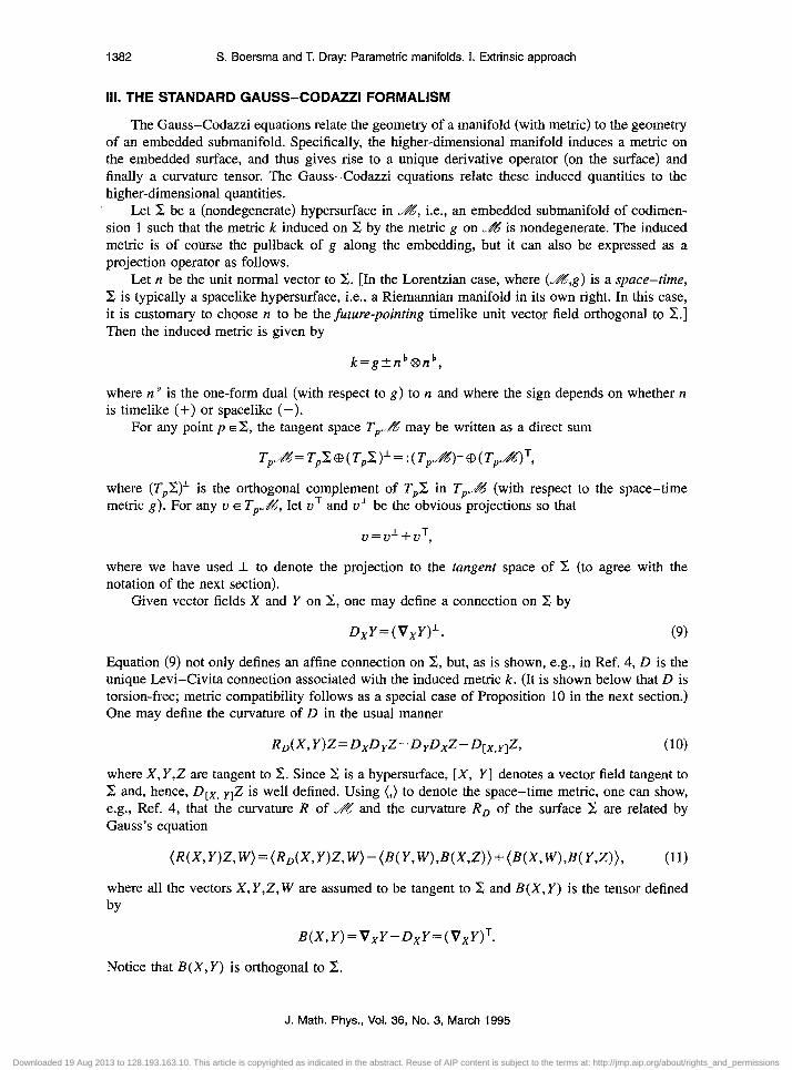
III. THE STANDARD GAUSS-CODA221 FORMALISM
The Gauss-Codazzi equations relate the geometry of a manifold (with metric) to the geometry of an embedded submanifold. Specifically, the higher-dimensional manifold induces a metric on the embedded surface, and thus gives rise to a unique derivative operator (on the surface) and finally a curvature tensor. The Gauss-Codazzi equations relate these induced quantities to the higher-dimensional quantities.
Let x be a (nondegenerate) hypersurface in 4, i.e., an embedded submanifold of codimen- sion 1 such that the metric k induced on 2 by the metric g on -8% is nondegenerate. The induced metric is of course the pullback of g along the embedding, but it can also be expressed as a projection operator as follows.
Let n be the unit normal vector to 2. [In the Lorentzian case, where (&,g) is a space-time, 2 is typically a spacelike hypersurface, i.e., a Riemannian manifold in its own right. In this case, it is customary to choose n to be the future-pointing timelike unit vector field orthogonal to x.1 Then the induced metric is given by
k=gfnb@nb,
where n b is the one-form dual (with respect to g) to n and where the sign depends on whether n is timelike (+) or spacelike (-).
For any point p ~2, the tangent space T,,A% may be written as a direct sum
where (T&)’ is the orthogonal complement of T$ in TP..,& (with respect to the space-time metric g). For any u E TPu&, let bT and Y’ be the obvious projections so that
lJ=vL+vT,
where we have used I to denote the projection to the tangent space of C (to agree with the notation of the next section).
Given vector fields X and Y on 2, one may define a connection on c by
DxY=(vxY)L. (9)
Equation (9) not only defines an affine connection on c, but, as is shown, e.g., in Ref. 4, D is the unique Levi-Civita connection associated with the induced metric k. (It is shown below that D is torsion-free; metric compatibility follows as a special case of Proposition 10 in the next section.) One may define the curvature of D in the usual manner
RD(X, Y)Z= DxDyZ- DyDxZ- Drx,ylZ, (10)
where X, Y,Z are tangent to 5. Since c is a hypersurface, [X, Y] denotes a vector field tangent to C and, hence, D,,, yl Z is well defined. Using (,) to denote the space-time metric, one can show, e.g., Ref. 4, that the curvature R of A?!? and the curvature RD of the surface 2 are related by Gauss’s equation
(R(X,Y)Z,W)=(RotX,Y)Z,W)-(B(Y,W),B(X,Z))+(B(X,W),B(Y,Z)), (11)
where all the vectors X, Y,Z, W are assumed to be tangent to 2 and B(X, Y) is the tensor defined by
Notice that B(X, Y) is orthogonal to C.
J. Math. Phys., Vol. 36, No. 3, March 1995
Downloaded 19 Aug 2013 to 128.193.163.10. This article is copyrighted as indicated in the abstract. Reuse of AIP content is subject to the terms at: http://jmp.aip.org/about/rights_and_permissions
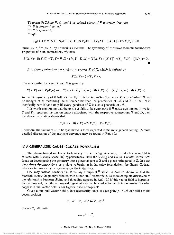
S. Boersma and T. Dray: Parametric manifolds. I. Extrinsic approach 1383
Theorem 8: Taking V, D, and B as dejined above, if V is torsion-free then (i) D is torsion-free and (ii) B is symmetric. Proof
T,(X,Y):=D,Y-D,X-[X, Y]=(V,Y)‘-(VyX)‘-[X, Y]=(T(X,Y))‘=O
since [X, Y]’ = [X, Y] by Frobenius’s theorem. The symmetry of B follows from the torsion-free properties of both connections. We have
B(X,Y)-B(Y,X)=V,Y-V,X-(D,Y-D,X)=(T(X,Y)+[X,Y])-(T,(X,Y)+[X,Y])=O. n
B is closely related to the extrinsic curvature K of z, which is defined by
K(X,Y)=(-V,Y,n).
The relationship between K and B is given by
K(X,Y)=(-VxY,n)=(-B(X,Y)-DxY,n)=(-B(X,Y),n)-(DxY,n)=(-B(X,Y),n)
so that the symmetry of K follows directly from the symmetry of B when V is torsion-free. B can be thought of as measuring the difference between the geometries of .&E’ and C. In fact, B is identically zero if (and only if) every geodesic of C is also a geodesic of &??.
It is worth mentioning that the tensor B fails to be symmetric if V possesses torsion. If we let T and T, represent the torsion tensors associated with the respective connections V and D, then the above calculation shows that
B(X,Y)-B(Y,X)=T(X,Y)-T&X,Y).
Therefore, the failure of B to be symmetric is to be expected in the most general setting. (A more detailed discussion of the extrinsic curvature may be found in Ref. 10.)
IV. A GENERALIZED GAUSS-CODAZZI FORMALISM
The above formalism lends itself nicely to the slicing viewpoint, in which a manifold is foliated with (usually spacelike) hypersurfaces. Both the slicing and Gauss-Codazzi formalisms focus on decomposing the geometry into a piece tangent to ‘c and a piece orthogonal to 2. One can view these decompositions as a place to begin an initial value formulation; the Gauss-Codazzi relations impose certain constraints on the initial data.
One may instead consider the threading viewpoint,” which is dual to slicing in that the manifold is now (regularly) foliated with a (non-null) vector field. (A more complete discussion of the relationship between slicing and threading appears in Ref. 12.) If this vector field is hypersur- face orthogonal, then the orthogonal hypersurfaces can be used as in the slicing scenario. But what happens if the vector field is not hypersurface orthogonal?
Given a non-null vector field A (not necessarily unit), at each point p in .& one still has the decomposition
T,&= ( T,L&)’ @ ( T+6%‘)T.
For u E Tp. &, write
J. Math. Phys., Vol. 36, No. 3, March 1995
Downloaded 19 Aug 2013 to 128.193.163.10. This article is copyrighted as indicated in the abstract. Reuse of AIP content is subject to the terms at: http://jmp.aip.org/about/rights_and_permissions
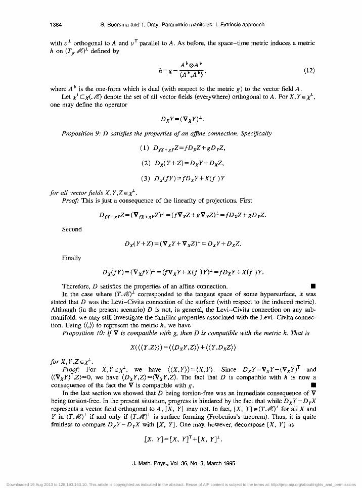
1384 S. Boersma and T. Dray: Parametric manifolds. I. Extrinsic approach
with u’ orthogonal to A and uT parallel to A. As before, the space-time metric induces a metric h on (T,..&)’ defined by
(12)
where A b is the one-form which is dual (with respect to the metric g) to the vector field A. Let xt Cx(J8) denote the set of all vector fields (everywhere) orthogonal to A. For X, Y E k,
one may define the operator
DxY=(VxY)‘.
Proposition 9: D satisfies the properties of an a&e connection. Speci$cally
(1) Dfx+srZ=fDxZ+gDyZ,
(2) Dx(Y+Z)=DxY+DxZ,
(3) PdfY)=fD,Y+X(f )Y
for all vectorjields X,Y,ZE~. Proof This is just a consequence of the linearity of projections. First
Dfx+$= (Vfx+g~Z)L = tfVxZ+gVyZ)l =fDxZ+gD,Z.
Second
Dx(Y+Z)=(VxY+VxZ)‘=DxY+DxZ.
Finally
D,(fY)=(VxfY)‘=(fVxY+X(f )Y)‘=fDxY+X(f )Y.
Therefore, D satisfies the properties of an affine connection. n In the case where (TJ&S’)~ corresponded to the tangent space of some hypersurface, it was
stated that D was the Levi-Civita connection of the surface (with respect to the induced metric). Although (in the present scenario) D is not, in general, the Levi-Civita connection on any sub- manifold, we may still investigate the familiar properties associated with the Levi-Civita connec- tion. Using ((,)) to represent the metric h, we have
Proposition 10: If V is compatible with g, then D is compatible with the metric h. That is
forX,Y,ZEti. Proof: For X,YE~, we have ((X,Y))=(X,Y). Since DxY=VxY-(V,Y)T and
((VxY)T,Z)=O, we have (D,Y,Z)=(V,Y,Z). The fact that D is compatible with h is now a consequence of the fact the V is compatible with g. n
In the last section we showed that D being torsion-free was an immediate consequence of V being torsion-free. In the present situation, progress is hindered by the fact that while DxY - D yX represents a vector field orthogonal to A, [X, Y] may not. In fact, [X, Y] E (T&5)’ for all X and Y in (T.4)’ if and only if (T.L&)’ is surface forming (Frobenius’s theorem). Thus, it is quite fruitless to compare DxY - D ,X with [X, Y]. One may, however, decompose [X, Y] as
[X, Y]=[X, r]T+[x, Y]l.
J. Math. Phys., Vol. 36, No. 3, March 1995
Downloaded 19 Aug 2013 to 128.193.163.10. This article is copyrighted as indicated in the abstract. Reuse of AIP content is subject to the terms at: http://jmp.aip.org/about/rights_and_permissions
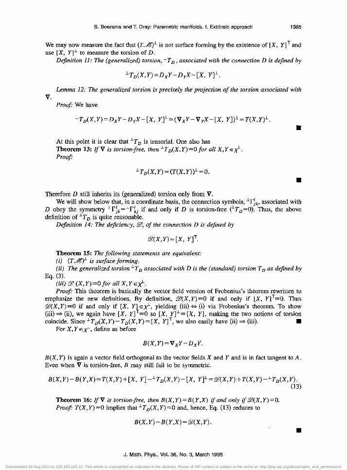
S. Boersma and T. Dray: Parametric manifolds. I. Extrinsic approach 1385
We may now measure the fact that (TL&)’ is not surface forming by the existence of [X, YIT and use [X, Y]’ to measure the torsion of D.
Definition 11: The (generalized) torsion, ‘To, associated with the connection D is de$ned by
‘T,(X,Y)=DxY-DyX-[X, Y]‘.
Lemma 12: The generalized torsion is precisely the projection of the torsion associated with V.
Proof We have
‘TD(X,Y)=DxY-DyX-[X, Y]‘=(V,Y-V,X-[X, Y])‘=T(X,Y)‘. n
At this point it is clear that ‘To is tensorial. One also has Theorem 13: If V is torsion-free, then ‘T,(X, Y) ~0 for all X, Y EX’. Proofi
‘Tb(X,Y)=(T(X,Y))‘=O. n
Therefore D still inherits its (generalized) torsion only from V. We will show below that, in a coordinate basis, the connection symbols, *I&, associated with
D obey the symmetry ‘l$=‘I$ if and only if D is torsion-free (‘Tb=O). Thus, the above definition of IT, is quite reasonable.
Definition 14: The deficiency, 3, of the connection D is defined by
S(X,Y) = [X, Y]T
Theorem 15: The following statements are equivalent: (i) (TL&?)~ is sugace forming. (ii) The generalized torsion ‘To associated with D is the (standard) torsion Tb as defined by
Eq. (3). (iii) LS(X,Y)=O for all X,Y ~2. Proof: This theorem is basically the vector field version of Frobenius’s theorem rewritten to
emphasize the new definitions. By definition, g(X,Y)=O if and only if [X, YIT=O. Thus sX,Y)=O if and only if [X, Y] Ed, yielding (iii) * (i) via Frobenius’s theorem. To show (iii) ==+ (ii), we again have [X, YIT=O so [X, Y]“=[X, Y], making the two notions of torsion coincide. Since ‘T&X, Y) - Tb(X, Y) = [X, YIT, we also easily have (ii) * (iii). n
For X, Y E ,$-, define as before
B(X,Y)=VxY-DXY,
B(X, Y) is again a vector field orthogonal to the vector fields X and Y and is in fact tangent to A. Even when V is torsion-free, B may still fail to be symmetric.
B(X,Y)-B(Y,X)=T(X,Y)+[X, Y] -‘T,(X,Y)-[X, Y]‘=.@(X,Y)+T(X,Y)-‘T,(X,Y). (13)
Theorem 16: IfV is torsion-free, then B(X, Y) = B( Y,X) if and only ifS@(X, Y) =O. Proofl T(X,Y)=O implies that *Tb(X,Y) =0 and, hence, Eq. (13) reduces to
B(X,Y)-B(Y,X)=S(X,Y). w
J. Math. Phys., Vol. 36, No. 3, March 1995
Downloaded 19 Aug 2013 to 128.193.163.10. This article is copyrighted as indicated in the abstract. Reuse of AIP content is subject to the terms at: http://jmp.aip.org/about/rights_and_permissions

1386 S. Boersma and T. Dray: Parametric manifolds. I. Extrinsic approach
We have that the deficiency of the connection D measures the failure of (T,&)’ to be surface forming and, equivalently, the failure of the extrinsic curvature B to be symmetric in a torsion-free setting. (Earlier work on projected connections and the second fundamental of nonintegrable plane fields may be found in Ref. 10.)
Being an affine connection, D must have an associated “curvature” tensor. However, the existence of the [X, YIT component prevents one from proceeding as before-“Dtx,yl” does not make sense! It appears as if this problem may be overcome simply by using the quantity [X, Y]’ to represent the commutator of two vector fields orthogonal to the original vector field A. Armed with such a notion of “bracket,” the next step would be to define a curvature operator.
De$nition 17: Dejne the operator S by
Unfortunately, such a definition immediately leads to problems. Proposition 18: S(X, Y)Z is notfunction linear (unless 3=0). That is,
(14)
S(X,fY)W) + fgW,W.
Proof:
W,f YNgZ) = @xCfDr) -fD@x- Dfix,rll -Dxcf ,r)(gz>
=fWLY)(gZ) + (Wf >Dr-Nf )D,)W) =fWL Y)kZ)
=f(Dx(Y(g)Z+gD,Z)-D,(X(g)Z+gDxz)-[X, Yl’kP-gDc,,y$)
=f ([X9 YlkP- LX, W(g)Z+ gw, W) =fsW, w+ 9(X, Y)(g)Z.
q
Therefore, in order to define a function linear curvature operator (tensor!), we must keep track of the [X, Y]’ component (we cannot just project it away and forget about it). That is, the Dfx,y~~Z term in Eq. (14) is not complete. We do not want to project the vector field [X, Y] too soon! We will, therefore, consider replacing the last term of Eq. (14) by the term (V,,, ylZ)L. This term is equivalent to the D,x,yl Z term in Eq. (10). However, since [X, Y] is not necessarily orthogonal to A we cannot write (VLx,ylZ)* in terms of the connection D.
Dejnition 19: The (generalized) curvature operator associated with D is dejined by
IR(X,Y)Z= D D Z-DyDxZ-(Vlx,y~Z)L. x y
Proposition 20: ‘R is function lineal: That is, ‘R is tensorial. Pro08
‘R(X,f Y)W) = @‘x(fDy) -fD@x- P~x,y]+ Vx, ,Y)%gZ)
=f’WU’HgZ)+Wf PY-O’X~)Y)%Z)
=fLRK Y&Z) I- (Wf Py--X(f P,)(gZ)
=f%C Y)(gZ)
=f(Dx(Y(g)Z+gDyz)--y(X(g)Z+gDxZ)-([X, WdZ+gVLx,y@) =fk*R(XW+[X YlkP-(CK Ylk)-G1) =fg%X, WC
J. Math. Phys., Vol. 36, No. 3, March 1995
Downloaded 19 Aug 2013 to 128.193.163.10. This article is copyrighted as indicated in the abstract. Reuse of AIP content is subject to the terms at: http://jmp.aip.org/about/rights_and_permissions
S. Boersma and T. Dray: Parametric manifolds. I. Extrinsic approach 1387
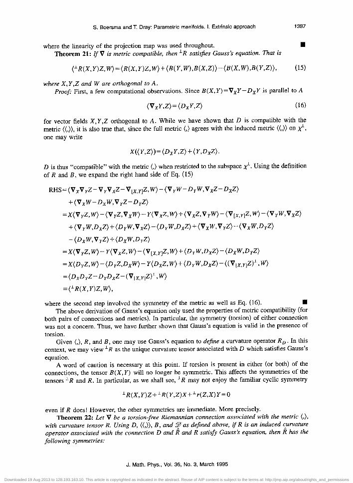
where the linearity of the projection map was used throughout. n Theorem 21: If V is metric compatible, then ‘R satis$es Gauss’s equation. That is
(‘RtX,Y)Z,W)=(R(X,Y)Z,W)+(B(Y,W),B(X,Z))-(BtX,W),BtY,Z)), (1%
where X, Y, Z and W are orthogonal to A. Proof First, a few computational observations. Since B(X, Y) =V,Y - D,Y is parallel to A
(W’,Z)=(D,Y,Z) (16)
for vector fields X, Y,Z orthogonal to A. While we have shown that D is compatible with the metric ((,)), it is also true that, since the full metric (,) agrees with the induced metric ((,)) on k, one may write
X((Y,Z))=(DxY,Z)+(Y,DxZ).
D is thus “compatible” with the metric (,) when restricted to the subspace 2. Using the definition of R and B, we expand the right hand side of Eq. (15)
-(DxWVyZ)+(DxW,D,Z)
where the second step involved the symmetry of the metric as well as Eq. (16). I The above derivation of Gauss’s equation only used the properties of metric compatibility (for
both pairs of connections and metrics). In particular, the symmetry (torsion) of either connection was not a concern. Thus, we have further shown that Gauss’s equation is valid in the presence of torsion.
Given (,), R, and B, one may use Gauss’s equation to define a curvature operator R, . In this context, we may view ‘R as the unique curvature tensor associated with D which satisfies Gauss’s equation.
A word of caution is necessary at this point. If torsion is present in either (or both) of the connections, the tensor B(X,Y) will no longer be symmetric. This affects the symmetries of the tensors ‘R and R. In particular, as we shall see, ‘R may not enjoy the familiar cyclic symmetry
‘R(X,Y)Z+‘R(Y,Z)X+‘r(Z,X)Y=O
even if R does! However, the other symmetries are immediate. More precisely. Theorem 22: Let V be a torsion-free Riemannian connection associated with the metric (,),
with curvature tensor R. Using D, ((,)), B, and qaas dejned above, if R is an induced curvature operator associated with the connection D and R and R satisfy Gauss’s equation, then R has the following symmetries:
J. Math. Phys., Vol. 36, No. 3, March 1995
Downloaded 19 Aug 2013 to 128.193.163.10. This article is copyrighted as indicated in the abstract. Reuse of AIP content is subject to the terms at: http://jmp.aip.org/about/rights_and_permissions

1388 S. Boersma and T. Dray: Parametric manifolds. 1. Extrinsic approach
(i) (i<X,Y)Z,W)=-(i(Y,X)Z,W), (ii) (li(X, Y)Z, W) = - (li(X, Y) W,Z), (iii) (jirst Bianchi identity)
(li(X,Y)Z+~(Y,Z)X+ii(Z,X)Y,W)=(B(X,W),~(Y,Z))+(B(Y,W),~(Z,X))
+(B(Z, W),9(X,Y))
=-(vxL2qY,z),w)-(vyB(z,x),w)
-(V&w,Y),W). (17)
Proof The symmetries in (i) and (ii) can be read off directly from Eq. (1 l), keeping in mind that R satisfies all of the symmetries of the usual Riemann curvature tensor (in the absence of torsion). To prove (iii), just cyclicly permute X, Y, and Z in the terms on the right hand side of Eq. (11) and add, obtaining
which is the first line in (iii). However, this cyclic sum involving B and Smay be rewritten in terms of V and a. Thus written, claim (iii) resembles the standard cyclic symmetry of R [see Eq. (S)]. Keep in mind, however, that neither V nor D possess torsion, although deficiency is present. We have
=x(w,qY,z))-(W,V,@(Y,Z))
= -(V,9?(Y,Z),W)
since 9( Y,Z) is orthogonal to W. Thus the second equation in (iii) is true. n Note that W is arbitrary in (i) and (iii), so that these can be rewritten in the same form as
Theorem 7 [except of course for the intermediate result in Eq. (17)]. One further comment on the similarities between Eqs. (8) and (17) is worth making. In Eq. (8)
there are three extra terms of the form T(X, [ Y, Z] ) (and cyclic permutations). One might expect analogous terms in Eq. (17) involving 9(X, [ Y, Z]‘) and cyclic permutations. However, since 3(X, Y) represents a vector field orthogonal to A
(%X,[Y, zllMv)=o. We see that the new concept of deficiency does indeed appear in the first Bianchi identity in just the way torsion would.
V. COORDINATE EXPRESSIONS
Let us now work in a coordinate patch and investigate the components of the above operators. For simplicity, we will consider the coordinate system inherited from a threading decomposition of space-time. (A more complete discussion of threading and its relationship to parametric manifolds appears in Ref. 12.) Let A be timelike (and C spacelike) with norm IAl = l/M, i.e.,
J. Math. Phys., Vol. 36, No. 3, March 1995
Downloaded 19 Aug 2013 to 128.193.163.10. This article is copyrighted as indicated in the abstract. Reuse of AIP content is subject to the terms at: http://jmp.aip.org/about/rights_and_permissions
S. Boersma and T. Dray: Parametric manifolds. I. Extrinsic approach 1389
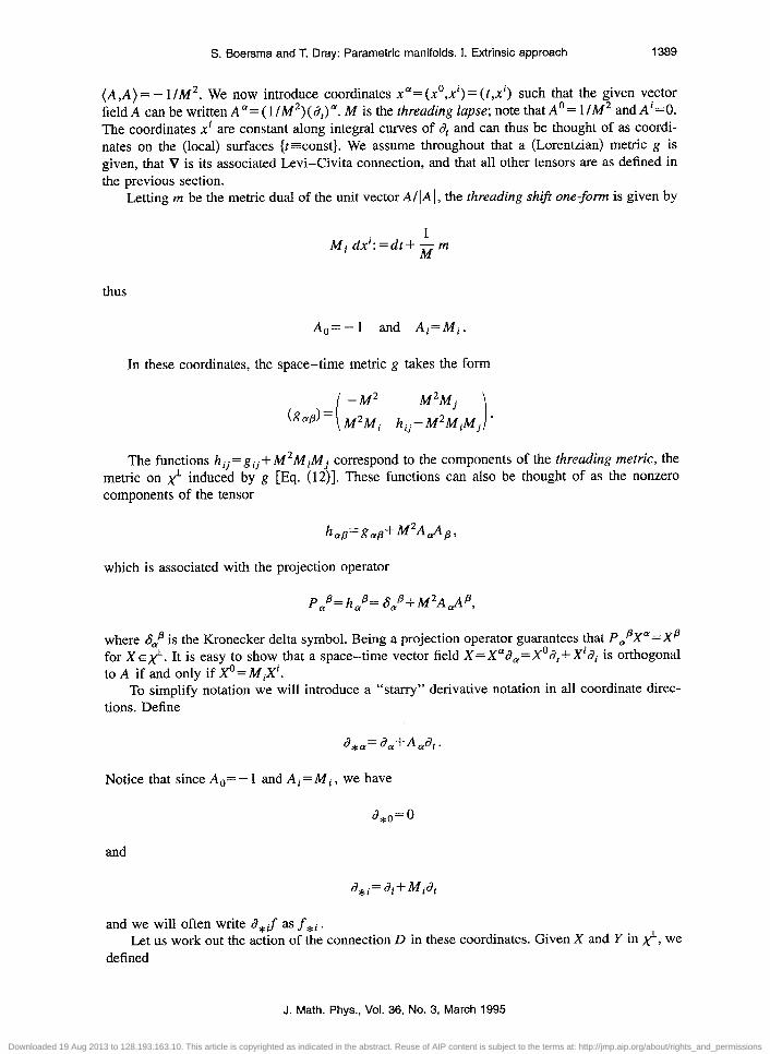
(A,A)= - l/M*. We now introduce coordinates xa= (x”,xi)=(t,xi) such that the given vector field A can be written A”= (l/M*)(d,)“. M is the threading lapse; note that A’= l/M* and A’=O. The coordinates xi are constant along integral curves of a, and can thus be thought of as coordi- nates on the (local) surfaces {t=const}. We assume throughout that a (Lorentzian) metric g is given, that V is its associated Levi-Civita connection, and that all other tensors are as defined in the previous section.
Letting m be the metric dual of the unit vector A/IA 1, the threading shzft one-form is given by
Mi dx’: =dt+ & m
thus
Ac=-1 and Ai=Mi.
In these coordinates, the space-time metric g takes the form
-M2 kYp) = M*Mi
The functions hij=gij+ M*MzMj correspond to the components of the threading metric, the metric on 2 induced by g [Eq. (12)]. These functions can also be thought of as the nonzero components of the tensor
which is associated with the projection operator
P/= h,P= CT/+ M*Adp,
where Sap is the Kronecker delta symbol. Being a projection operator guarantees that PaBXa= Xp for XE~. It is easy to show that a space-time vector field X=Xad,=Xoa,+Xid)i is orthogonal to A if and only if X0= Mix’.
To simplify notation we will introduce a “starry” derivative notation in all coordinate direc- tions. Define
a *a= d,+A,dz .
Notice that since A,= - 1 and Ai= Mi, we have
d*o=O
and
and we will often write 6’,J as f*i . Let us work out the action of the connection D in these coordinates. Given X and Y in 2, we
defined
J. Math. Phys., Vol. 36, No. 3, March 1995
Downloaded 19 Aug 2013 to 128.193.163.10. This article is copyrighted as indicated in the abstract. Reuse of AIP content is subject to the terms at: http://jmp.aip.org/about/rights_and_permissions
1390 S. Boersma and T. Dray: Parametric manifolds. I. Extrinsic approach
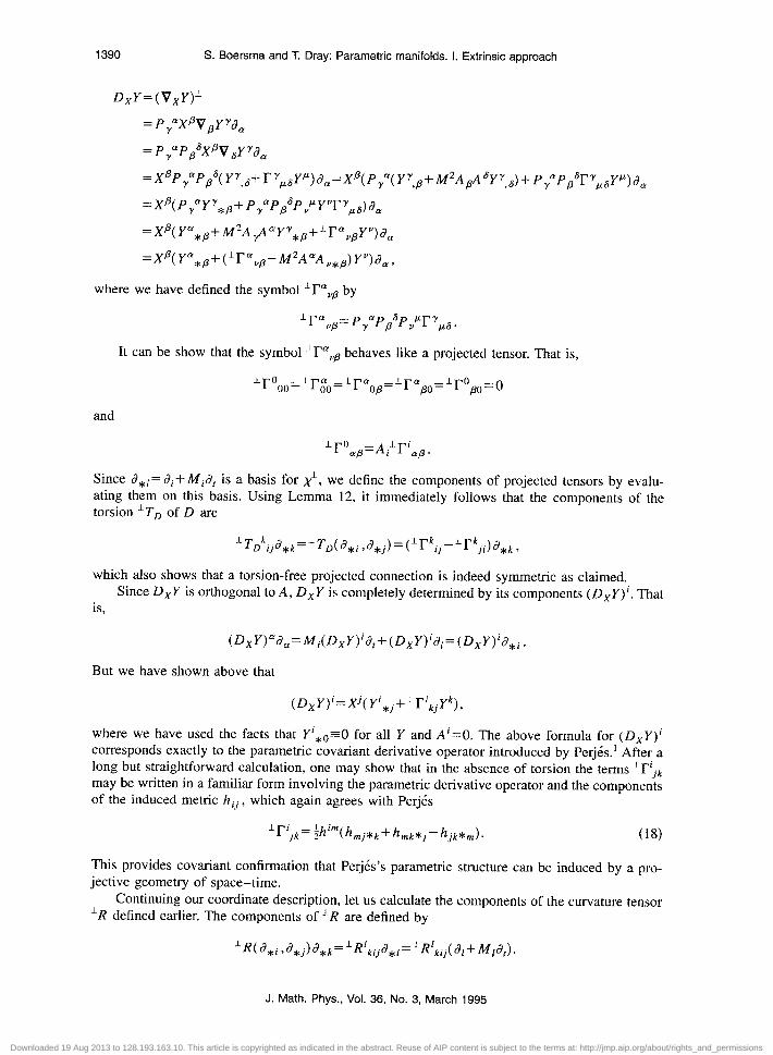
DxY=(v,Y)’
= P,“XQpYYd,
= P,aPpsX47sYYd,
=XPP~~P~~(Y~,~+T’~~Y’L)~,=X~(P~~(Y~,~+M*A~~Y~.~)+P~~P~~~~~~Y~)~~
=xq PraYY*p + P,*Pp*P”~Y”rQ)d,
= xq Ya *p+M2A~PYY,p+‘r”vpY”)d,
= xq Y” *P+(‘Ta”p-M2AaAY*B)YY)dn,
where we have defined the symbol iTa,,p by
lrff vp= p,~ppsp,~r~ps. It can be show that the symbol ‘I? Vp behaves like a projected tensor. That is,
and
1r-O ap=Aiiriap.
Since d*i=di+ Mid, is a basis for 2, we define the components of projected tensors by evalu- ating them on this basis. Using Lemma 12, it immediately follows that the components of the torsion ‘TD of D are
which also shows that a torsion-free projected connection is indeed symmetric as claimed. Since D,Y is orthogonal to A, D,Y is completely determined by its components (D,Y)‘. That
is,
But we have shown above that
where we have used the facts that Y’ *o=O for all Y and A’=O. The above formula for (D,Y)’ corresponds exactly to the parametric covariant derivative operator introduced by Perjes.’ After a long but straightforward calculation, one may show that in the absence of torsion the terms ‘rijk may be written in a familiar form involving the parametric derivative operator and the components of the induced metric hij , which again agrees with Perjds
‘rijk=~him(hmj*k+h,k*j-hjk*m). (18)
This provides covariant confirmation that Perjes’s parametric structure can be induced by a pro- jective geometry of space-time.
Continuing our coordinate description, let us calculate the components of the curvature tensor ‘R defined earlier. The components of LR are defined by
J. Math. Phys., Vol. 36, No. 3, March 1995
Downloaded 19 Aug 2013 to 128.193.163.10. This article is copyrighted as indicated in the abstract. Reuse of AIP content is subject to the terms at: http://jmp.aip.org/about/rights_and_permissions
S. Boersma and T. Dray: Parametric manifolds. 1. Extrinsic approach 1391
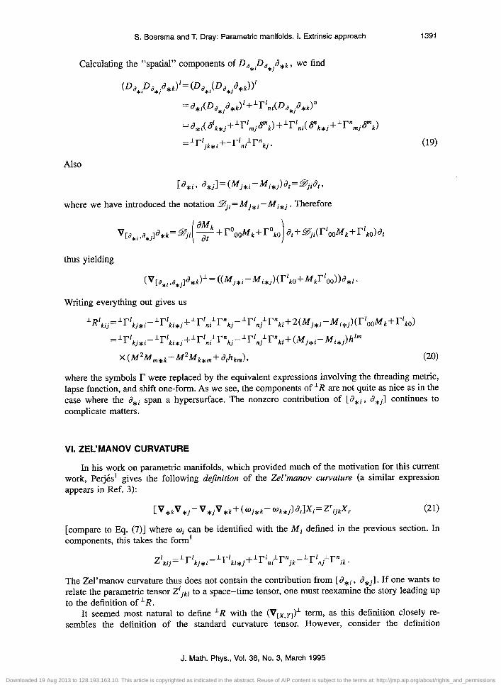
Calculating the “spatial” components of Dd,iDd,j6’*k, we find
(&*iD,*j&,)l= (D,,iU’,.+j6+d1
=d*i(Da,jd*k)i+~rl,i(D,*ja,,)”
=d*i( #k*jfLrlmjflk)fLrlni( gk.+j+‘rnmjflk)
=~r~jk*i+~r~ni~r~ kj * (19)
Also
where we have introduced the notation ~ji= Mj*i- Mi*j . Therefore
thus yielding
Writing everything out gives us
‘R’kij=‘rlkj*i-‘r’ki*j +‘rz~i’rnkj-‘r’nj~rnki+2(Mj*i-Mi*j)(r100Mk+r’kO)
“rlkj*i-lrlki*j+‘rl,j’rnkj- ‘rlnj’rnki+(Mj*i-Mi*j)h’m
x (M2Mm,k-M2Mk+ + &m) 9 (20)
where the symbols IT were replaced by the equivalent expressions involving the threading metric, lapse function, and shift one-form. As we see, the components of ‘R are not quite as nice as in the case where the d,i span a hypersurface. The nonzero contribution of [ d*i , d*j] continues to complicate matters.
VI. ZEL’MANOV CURVATURE
In his work on parametric manifolds, which provided much of the motivation for this current work, Perjis’ gives the following definition of the Zel’manov curvature (a similar expression appears in Ref. 3):
[V*kV*j-V*jV*k+(Wj*k-Ok*j)dtlXi=ZrijkX, (20
[compare to Eq. (7)] h w ere wi can be identified with the Mi defined in the previous section. In components, this takes the form’
z’ ..=lrl ku
.- k/*1 Lr’ki*j +*p ,lp, -lrl
nt Jk .lrn.
nJ zk .
The Zel’manov curvature thus does not contain the contribution from [ d*i , d*j] . If one wants to relate the parametric tensor zijk[ to a space-time tensor, one must reexamine the story leading Up to the definition of ‘R.
It seemed most natural to define ‘R with the (VLx,rl)L term, as this definition closely re- sembles the definition of the standard curvature tensor. However, consider the definition
J. Math. Phys., Vol. 36, No. 3, March 1995
Downloaded 19 Aug 2013 to 128.193.163.10. This article is copyrighted as indicated in the abstract. Reuse of AIP content is subject to the terms at: http://jmp.aip.org/about/rights_and_permissions
1392 S. Boersma and T. Dray: Parametric manifolds. I. Extrinsic approach
9?(X,Y)Z=Dx y D Z-D,D,Z-DL,,,I~Z-[~(X,Y),Z]l (22)
which can easily be shown to be function linear in its arguments, and thus defines a tensor (This is the same as the curvature operator defined by Lottermoser.13 It can also be written %(X,Y)Z= D,D,Z- D,D,Z-(29 lx,rlZ)’ -D,[X, Y]‘.) The difference between these two cur- vature operators is
lR(X, Y)Z-qx, Y)Z= - (V,B(X, Y))l (23)
(assuming V is torsion-free). In light of our earlier comments, we know that Ii? does not in general satisfy Gauss’s equation. Note that if (T&)’ is surface forming, so that [d,i, d,j] =0 (or equivalently @=O), then ‘R = ’ R.
We now show that we have in fact defined the Zel’manov curvature. Theorem 23: ‘R is the Zel’manov curvature. Proof: Using EQ. (19) and the facts that
we have
(24) n
VII. DISCUSSION
The generalized Gauss-Codazzi approach seems to have been successful in defining a notion of projected connection D, with a corresponding notion of torsion. Moreover, D was found to be torsion-free if V was torsion-free. Most importantly, the deficiency %J was explicitly defined in such a way as to make its relationship to the torsion tensor clear. While distinct from torsion, deficiency plays much the same role, e.g., in the first Bianchi identity. (While we have not yet checked explicitly, we expect the same will be true for the Codazzi equation and the second Bianchi identity.) The recent work of Gowdy14 also introduced notions of such projected covariant derivatives and “torsion” tensors.
However, there is one very peculiar aspect of this formalism, namely, the absence of an embedded hypersurface c to which to project! We have chosen to interpret the Gauss-Codazzi formalism as providing a pointwise projection, so that one obtains tensor fields defined on all of 4, rather than on a preferred hypersurface C.
If the orthogonal hypersurfaces in the standard setting are diffeomorphic to each other, then all projected tensors can be viewed as living on the same such hypersurface, but at different “times.” This viewpoint lends itself well to initial value problems. But this viewpoint also carries over to our generalized framework, the only change being that one must work on the manifold of orbits of the foliation, which is now assumed to be diffeomorphic to any hypersurface of constant “time.” Note that regularity of the foliation does not guarantee that the orthogonal hypersurfaces are diffeomorphic to the manifold of orbits. This can easily be seen by considering a simple example such as the Minkowskian cylinder with a rotating observer. In such a case the orthogonal surfaces are helices, but the manifold of orbits is a circle, so that they are at best locally diffeomotphic.
A parametric manifold is, in this setting, the manifold of orbits, on which there are one- parameter families of projected tensor fields. The geometric nature of its construction, using orthogonal projection, ensures that it is reparameterization invariant, i.e., that it is invariant under the special coordinate transformations which relabel “time.” This notion of one-parameter fami- lies of tensor fields together with a suitable reparameterization invariance can be used to give an intrinsic description of a parametric manifold, without using projections; this will be published separately.15 The notion of a parametric manifold is related to some recent work by Harris and
J. Math. Phys., Vol. 36, No. 3, March 1995
Downloaded 19 Aug 2013 to 128.193.163.10. This article is copyrighted as indicated in the abstract. Reuse of AIP content is subject to the terms at: http://jmp.aip.org/about/rights_and_permissions
S. Boersma and T. Dray: Parametric manifolds. I. Extrinsic approach 1393
co-workers on orbit spacesn’ and static space-times.17 Finally, we note that we have two somewhat different candidates, ‘R and Z, for the curvature
of our projected connection. The difference between the two involves the deficiency, and hence vanishes in the hypersurface-orthogonal case. More importantly, the difference also involves the lapse function M, which relates our arbitrary parameter t to arc length (proper “time”) along the given curves. For a given problem, which of these notions of curvature is “correct” may thus depend on whether a notion of distance orthogonal to the manifold of orbits is appropriate.
This brings us to the use of the Gauss-Codazzi formalism in initial value problems, especially in general relativity. The initial value formulation of Einstein’s equations imposes (consequences of’) the Gauss-Codazzi equations as constraints (and then uses the Mainardi equations to deter- mine the evolution). We thus conjecture that our framework can be used to generalize the initial value formulation for Einstein’s equations to appropriate data on the manifold of orbits. We further conjecture that it is precisely the (generalized) Gauss and Codazzi equations which will lead to the appropriate constraints. This would also provide some evidence in favor of ‘R, which does satisfy Gauss’s equation, rather than Z, which does not. We are actively pursuing these ideas.
ACKNOWLEDGMENTS
It is a pleasure to thank Bob Jantzen and Zoltan Perjis for their encouragement throughout this project, which builds on earlier results of theirs. We also extend thanks to Pawel Walczak for his comments. Furthermore, our many discussions with Jim Isenberg, Juha Pohjanpelto, and J&g Frauendiener proved to be invaluable. This work forms part of a dissertation submitted to Oregon State University (by S.B.) in partial fulfillment of the requirements for the Ph.D. degree in math- ematics.
This work was partially funded by NSF Grant No. PHY-9208494.
‘2. Perjks, “The parametric manifold picture of space-time,” Nucl. Phys. B 403, 809 (1993). *A. Zel’manov, Sov. Phys. Dokl. 1, 227-230 (1956). 3A. Einstein and P Bergmann, Ann. Math 39, 683-701, (1938); this article was reprinted in Introduction to Modern
Kuluzu-Klein Theories, edited by T. Applequist, A. Chodos, and P. G. 0. Freund (Addison-Welsey, Menlo Park, 1987). 4M. do C-0, Riemannian Geometry, translated by F. Flaherty (Birkhluser, Boston, 1992). ‘R. Bishop and S. Goldberg, Tensor Analysis On Manifolds (Dover, New York, 1980). ‘B. O’Neill, Semi-Riemannian Geometry with Applications to Relativiry (Academic, Orlando, 1983). ‘S. Kobayashi and K. Nomizu, Foundations of Differential Geometry (Wiley, New York, 1963), Vol. I. sR. Wald, General Relativity (University of Chicago, Chicago, 1984). 9M. Spivak, A Comprehensive Introduction to Differential Geometry (Publish or Perish, Houston, 1979), Vol. II.
“B. L. Reinhart, “The second fundamental from of a plane field,” J. Diff. Geom. 12, 619-627, (1977); Differential Geometry of Foliations (Springer-Verlag, New York, 1980).
“R. Jantzen and P. Carini, “Understanding space-time splittings and their relationships, ” in Classical Mechanics and Relativity: Relationship and Consistency, edited by G. Ferrarese (Bibliopolis, Naples, 1991), pp. 185-241; R. Jantzen, P. Carini, and D. Bini, “The many faces of gravitoelectromagnetism,,” AM. Phy. (NY) 215, l-50 (1992).
“S. Boersma and T. Dray, “Slicing, threading, and parametric manifolds,” Gen. Relativ. Gravit. (to appear). 13M. Lottermoser, “iiber den Newtonschen Grenzwert der Allgemeinen Relatividtstheorie und die relativistische Erweit-
erung Newtonscher Anfangsdaten,” Dissertation der Fakultat fur Physik der Ludwig-Maximilians-Universitit Miinchen, 1988.
14R. H. Gowdy, “Aftine projection tensor geometry: Lie derivatives and isometrics,” Preprint gr-qc/9408014; J. Math. Phys. 35, 1274-1301 (1994).
I5 S. Boersma and T. Dray, “Parametric manifolds. II. Intrinsic approach,” J. Math. Phys. 36, 1394-1403 (1995), following paper.
16S. G. Harris and R. J. Low, “Causal monotonicity and the Spahe of space” (in preparation); “Causality conditions and Hausdorff orbit spaces” (to appear in Proceedings of the Geometry Conference at Katholieke Universiteit, Leuven and Brussels, Festschrift Nomizu, 1994); “The method of timelike two-surfaces,” in Differential Geometry and Muthemati- cal Physics, Contemporary Mathematics, Vol. 170, edited by J. K. Beem and K. Duggal (American Mathematical Society, Providence, 1994).
“S G Harris and D. Garfinkle, “Ricci fall-off in static, globally hyperbolic, geodesically complete, Ricci-positive space- times” (to appear in Proceedings of the 7th Marcel Grossman Conference on General Relativity); D. Garfinkle and S. G. Harris, “Ricci fall-off and the static observer space in the absence of singularities” (in preparation).
J. Math. Phys., Vol. 36, No. 3, March 1995
Downloaded 19 Aug 2013 to 128.193.163.10. This article is copyrighted as indicated in the abstract. Reuse of AIP content is subject to the terms at: http://jmp.aip.org/about/rights_and_permissions