Stokes manifolds and cluster algebras - arXiv

Stokes manifolds and cluster algebrasM. Bertola†‡1, S. Tarricone†♦ 2,

† Department of Mathematics and Statistics, Concordia University1455 de Maisonneuve W., Montreal, Quebec, Canada H3G 1M8

‡ SISSA/ISAS, Area of Mathematicsvia Bonomea 265, 34136 Trieste, Italy

♦ LAREMA, UMR 6093, UNIV Angers, CNRS, SFR Math-Stic, France

Abstract

Stokes’ manifolds, also known as wild character varieties, carry a natural symplectic structure. Our goal isto provide explicit log-canonical coordinates for these natural Poisson structures on the Stokes’ manifolds ofpolynomial connections of rank 2, thus including the second Painleve hierarchy. This construction providesthe explicit linearization of the Poisson structure first discovered by Flaschka and Newell and then redis-covered and generalized by Boalch. We show that, for a connection of degree K, the Stokes’ manifold isa cluster manifold of type A2K . The main idea is then applied to express explicitly also the log–canonicalcoordinates for the Poisson bracket introduced by Ugaglia in the context of Frobenius manifolds and thenalso applied by Bondal in the study of the symplectic groupoid of quadratic forms.

Contents

1 Introduction and results 1

2 Symplectic structure on Stokes’ matrices 4

3 Stokes manifolds for n = 2 113.1 Computation of WK . . . . . . . . . . . . . . . . . . . . . . . . . . . . . . . . . . . . . . . . . 113.2 Comparison between PK and Poisson structure on Y -cluster manifold . . . . . . . . . . . . . 183.3 Flipping the edges . . . . . . . . . . . . . . . . . . . . . . . . . . . . . . . . . . . . . . . . . . 203.4 Example: the case K = 2 . . . . . . . . . . . . . . . . . . . . . . . . . . . . . . . . . . . . . . 243.5 Computation of the Poisson brackets for the original monodromy parameters . . . . . . . . . 25

4 Log canonical coordinates for the Ugaglia bracket 28

5 Conclusion and outlook 31

A Proof of Prop. 3.14 32

1 Introduction and results

Rational connections on the Riemann sphere (and more general Riemann surfaces) are intimately connectedwith the theory of integrable systems in general, and Painleve equations in particular (or Hitchin’s systems).

The (generalized) monodromy map which associates the monodromy, Stokes’ and connection matricesto a rational connection, has been shown to provide integrals of motion for all the Painleve equations (andhence parametrize their solutions) and the generalizations thereof that culminated in the eighties with thework of the Japanese school [16, 17, 18].

The Painleve equations themselves can be cast as Hamiltonian systems [24]; the underlying Poissonstructure coincides with the standard Poisson structure on coadjoint orbits of suitably defined loop groups[1].

[email protected], [email protected], [email protected]

1

arX

iv:2

104.

1378

4v1

[m

ath.

SG]

28

Apr

202

1

The (extended) monodromy map provides a connection between these ODE (rational connections) andthe representations theory of the fundamental group of the punctured sphere, which are called “charactervarieties” (for the case of Fuchsian singularities) or certain generalizations thereof that go under the pic-turesque name of “wild character varieties” [22].

The natural question, from the point of view of symplectic geometry, is to identify the push–forward ofthe Poisson structure from the space of coadjoint orbits to the space of extended monodromy data.

Possibly the first paper to address this issue was [12] in the eighties; they considered the prototypicalexample of “wild” character variety, namely, the Stokes’ phenomenon of a rank-two differential equation withpolynomial coefficients , which underlies the Painleve II hierarchy. They provided the explicit expressions forthe Poisson brackets between the Stokes’ parameters which are the image, under the generalized monodromymap, of the Lie-Poisson structure on the matrix of the differential equation.

On a similar track, but for the regular monodromy map, in the work [19] it was first realized that theLie-Poisson structure on a Fuchsian differential connection induces the Goldman Poisson structure [15] onthe matrices of the monodromy representation.

The seminal paper of Flaschka and Newell was largely ignored for almost twenty years and then its ideaapplied to a different type of rational connections by Ugaglia [25] in relationship with the theory of Frobeniusmanifolds; here the connection has one Fuchsian and one irregular singularity of Poincare rank 2 at infinity.

The topic was then put into the framework of quasi–Hamiltonian geometry in a series of papers by Boalch[6, 7, 8] in the beginning of the millennium, where he re-derived the symplectic and Poisson geometry inducedon the space of generalized monodromy data.

A practical issue that has not been given much consideration until lately, is that of providing explicitDarboux coordinates (or, rather, log-canonical) for these structures; in the last decade the works of Fock-Goncharov [13] have shown the connection between the geometry of character varieties and the emergentstudy of cluster algebras. Their setup is very general but phrased in a setting which is abstracted from thedirect relationship with the theory of the monodromy map.

In the recent [5] the Fock-Goncharov formalism has been shown to provide explicit log-canonical co-ordinates for the Goldman Poisson structure on the character variety of an arbitrary punctured Riemannsurface.

The relationship of the Fock–Goncharov coordinates with the Stokes’ phenomenon of second order ODEson Riemann surfaces was pointed out in [23]; however this relationship is for a different Stokes’ phenomenon,corresponding to the Wentzel-Kramers-Brillouin asymptotic expansion with respect singularly perturbedODEs.

The present paper instead considers the classical Stokes’ phenomenon for (polynomial) ODEs and pro-vides explicit log-canonical (and Darboux) coordinates for the Poisson structure on the simplest class of suchwild character varieties. We thus establish the main result that can be summarized in the following theorem

Theorem. The wild character variety of an sl2 polynomial connection of degree K on the Riemann sphereis a cluster manifold of type A2K . The log–canonical Poisson (symplectic) structure on this cluster varietycoincides with the push–forward by the monodromy map of the Lie-Poisson structure.

Detailed description of results. In Section 2 we provide a self–contained explanation of the symplecticstructure on Stokes’ matrices associated to an arbitrary polynomial differential equation in sln; the result(in even greater generality) was derived by Boalch [8], generalizing the result of [12] and [25]. The proof weprovide, however, is completely different from loc. cit. and uses ideas developed around the notion of theMalgrange one-form in [3, 4].

We then consider in detail the case of sl2 polynomial differential equation of arbitrary Poincare rankK + 1. The goal is to provide explicit parametrizations for the Stokes’ parameters and to show that thecoordinate charts thus defined glue together in the fashion of a cluster manifold of type A2K . We recall thatthe Stokes’ manifold in this case consists in the following algebraic variety

SK =

(1 s1

0 1

)(1 0s2 1

). . .

(1 s2K+1

0 1

)(1 0

s2K+2 1

)λσ3 = 1 with si ∈ C, λ ∈ C×

(1.1)

of complex dimension 2K (here and below σ1,2,3 denote the three Pauli matrices).

2

The results of [12] can be summarized in the following Poisson brackets (see Def. 3.13):sj , sl

FN

= δj,l−1 −δj,1δl,2K+2

λ2+ (−1)j−l+1sjsl, j < l.

sj , λFN

= (−1)jsjλ. (1.2)

It is interesting here to observe that the brackets (1.2) satisfy the Jacobi identity in fact on the manifoldof dimension 2K + 3 consisting of the parameters sj ’s and λ without any restriction, where it has a singleCasimir function given by the trace of the product in the left hand side of the equality in (1.1). Thevariety SK is a Poisson submanifold and the bracket becomes nondegenerate (see Prop. 3.14) The explicitparametrization of the Stokes’ data on the constrained manifold (1.1) is given by (see Lemma 3.5)

s1 = −y−21

s2k = (1 + y22k)

∏1≤j≤2k

y(−1)j+12j , k = 1, . . . ,K

s2k+1 = −(1 + y22k+1)

∏1≤j≤2k+1

y(−1)j2j , k = 1, . . . ,K − 1

s2K+1 = −∏

1≤j≤2K

y(−1)j2j ,

s2K+2 = y21

(1 + y2

2

(. . .(1 + y2

2K

). . .)) K∏

j=1

y−42j ,

λ =

K∏j=1

y22j .

and these coordinates y1, . . . , y2K are log–canonical; the matrix of their Poisson brackets is (Lemma 3.7)

PK =1

4

0 1 0 0 0 . . . 0−1 0 1 0 0 . . . 00 −1 0 1 0 . . . 0...

. . .. . .

. . ....

.... . .

. . .. . .

...0 0 . . . −1 0 10 0 . . . 0 −1 0

(1.3)

The particular parametrization described here corresponds to a certain triangulation (see Fig. 5) of the2(K + 1) regular polygon, much in the same way as the relationship between the Grassmannian of 2-planes([14], Ch. II). The reader versed in the theory of cluster algebras will then recognize in the matrix abovethe matrix representing the simple quiver of type A2K ; this means that the variables y2

j form a seed for thecluster algebra of type A2K .

To complete the picture we need to show that different choices of triangulations of the regular 2K + 2–gon yield parametrizations of the Stokes’ data that are obtained from the initial seed by applying a suitablesequence of mutations , i.e. simple birational maps from one chart to another. This is accomplished in Sec.3 and specifically Sec. 3.3. We prove (Thm. 3.15) that the Flaschka–Newell Poisson bracket coincides withthe described above.

To conclude, in Sec. 4 we provide, using the same ideas used in the main text, the explicit log-canonicalcoordinates for the Poisson bracket introduced in [25]. This construction provides an alternative approachto the recent work by Checkov and Shapiro [10].

3

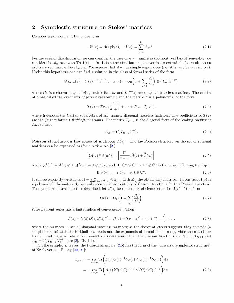
2 Symplectic structure on Stokes’ matrices

Consider a polynomial ODE of the form

Ψ′(z) = A(z)Ψ(z), A(z) :=

K∑j=1

Ajzj . (2.1)

For the sake of this discussion we can consider the case of n×n matrices (without real loss of generality, weconsider the sln case with Tr(A(z)) ≡ 0). It is a technical but simple exercise to extend all the results to anarbitrary semisimple Lie algebra. We assume that AK has simple eigenvalues (i.e. it is regular semisimple).Under this hypothesis one can find a solution in the class of formal series of the form

Ψform(z) = Y (z)z−LeT (z), Y (z) := G0

(1 +

∑j≥1

Yjzj

)∈ SLn[[z−1]], (2.2)

where G0 is a chosen diagonalizing matrix for AK and L, T (z) are diagonal traceless matrices. The entriesof L are called the exponents of formal monodromy and the matrix T is a polynomial of the form

T (z) = TK+1zK+1

K + 1+ · · ·+ T1z, Tj ∈ h, (2.3)

where h denotes the Cartan subalgebra of sln, namely diagonal traceless matrices. The coefficients of T (z)are the (higher formal) Birkhoff invariants. The matrix TK+1 is the diagonal form of the leading coefficientAK , so that

AK = G0TK+1G−10 . (2.4)

Poisson structure on the space of matrices A(z). The Lie Poisson structure on the set of rationalmatrices can be expressed as (for a review see [2])

A(z)⊗, A(w) =

[Π

z − w,1

A(z) +2

A(w)

](2.5)

where A1(z) := A(z)⊗ 1, A2(w) := 1⊗A(w) and Π : Cn ⊗ Cn → Cn ⊗ Cn is the tensor effecting the flip:

Π(v ⊗ f) = f ⊗ v, v, f ∈ Cn. (2.6)

It can be explicitly written as Π =∑nk,j=1 Ek,j ⊗Ej,k, with Eij the elementary matrices. In our case A(z) is

a polynomial; the matrix AK is easily seen to consist entirely of Casimir functions for this Poisson structure.The symplectic leaves are thus described; let G(z) be the matrix of eigenvectors for A(z) of the form

G(z) = G0

(1 +

∑j≥1

Bjzj

). (2.7)

(The Laurent series has a finite radius of convergence). Then

A(z) = G(z)D(z)G(z)−1, D(z) = TK+1zK + · · ·+ T1 −

L

z+ . . . (2.8)

where the matrices Tj are all diagonal traceless matrices; as the choice of letters suggests, they coincide (asimple exercise) with the Birkhoff invariants and the exponents of formal monodromy, while the rest of theLaurent tail plays no role in our present considerations. Then the Casimir functions are T1, . . . , TK+1 andAK = G0TK+1G

−10 . (see [2], Ch. III).

On the symplectic leaves, the Poisson structure (2.5) has the form of the “universal symplectic structure”of Krichever and Phong [20, 21]:

ωKK

= − resz=∞

Tr

(D(z)G(z)−1δG(z) ∧G(z)−1δG(z)

)dz

= − resz=∞

Tr

(A(z)δG(z)G(z)−1 ∧ δG(z)G(z)−1

)dz (2.9)

4

The two form is invariant under gauge action of right multiplication of G by diagonal matrices of the form

F (z) = 1 +∑j≥1

Fjzj

∈ h[[z−1]]. (2.10)

To see this we introduce the symplectic potential

θ := resz=∞

Tr

(D(z)G(z)−1δG(z)

)(2.11)

which has the property that δθ = ωKK

. Now observe that under the gauge transformation G(z) 7→ G(z)F (z)we have

θ 7→ θ + resz=∞

Tr

(D(z)F−1(z)δF (z)

)dz. (2.12)

In the latter term, since F (z) = 1 + O(z−1) only the non-negative powers of D(z) contribute (sinceF−1(z)δF (z) = O(z−1)). Given that the parameters T1, . . . , TK+1 in (2.8) are constants, we can express thelast term in (2.12) as the total derivative of the function

resz=∞

Tr

(D(z)F−1(z)δF (z)

)dz = δ res

z=∞Tr

(D(z) lnF (z)

)dz, (2.13)

which implies that ωKK

= δθ is indeed invariant. It is also invariant under left multiplication G(z) 7→ HG(z)with H a constant (in z): indeed, the left multiplication by a constant matrix H leaves θ completely invariant:

θ 7→ θ + resz=∞

Tr

(G(z)D(z)G−1(z)H−1δH

)dz = θ (2.14)

where we have used that G(z)D(z)G−1(z) = A(z) is a polynomial.The core of the idea of the “extended coadjoint orbit” of [8] is the following: while AK = G0TK+1G

−10

is a Casimir for the KKS symplectic structure, G0 itself is not because right multiplications by a constantdiagonal matrix do not leave the symplectic form invariant.

Thus we allow G0 to be kinematical variables: fix the Birkhoff invariants T (z) =∑K+1j=1 Tjz

j/j (i.e. thediagonal traceless matrices T1, . . . , TK+1) and consider the set

OT :=

(G0, A(z)) ∈ SLn ×AK : G−1

0 AKG0 = TK+1, (G(z)−1A(z)G(z))+ = T ′(z)

, (2.15)

where ()+ denotes the Taylor part of a Laurent series (here is a polynomial part).

The dimension of OT is

dimC

(OT)

= (K + 1)(n2 − 1) + (n− 1)− (K + 1)(n− 1) = Kn(n− 1) + n2 − 1 (2.16)

The extended orbit OT carries the following SLn–action:

(G0, A(z)) 7→ (HG0, HA(z)H−1), H ∈ SLn. (2.17)

Then the quotient OT /SLn is a symplectic manifold of dimension Kn(n− 1) = dimC SK .

In order to connect the Lie–Poisson structure with the Flaschka–Newell structure on the Stokes’ matriceswe need first a lemma and to describe the Stokes’ phenomenon.

Lemma 2.1. The first K+1 coefficient matrices Y1, . . . , YK+1 in the expansion of the formal solution Ψform

(2.2) coincide with the expansion of the eigenvector matrix, to wit

Y (z) := G0

1 +∑j≥1

Yjzj

= G(z) +O(z−K−2). (2.18)

5

Proof. The formal series Y satisfies the ODE

Y ′(z) + Y (z)

(T ′(z)− L

z

)= A(z)Y (z). (2.19)

Since Y ′(z) = O(z−2), the matrices T (z), L are diagonal and since the degree of A is K we deduce that Ymatches the Laurent expansion of the eigenvector matrix G(z) up to the indicated order.

Description of the Stokes’ phenomenon (extended monodromy map). The plane can be parti-tioned into 2K + 2 sectors of equal angular width Sµ, arranged in counterclockwise order ; within each suchsector, there exists a unique analytic solution Ψµ(z) to the ODE 2.1 such that [26]

Ψµ(z) ' Ψform(z), |z| → ∞, arg z ∈ Sµ, (2.20)

with Ψform given in (2.2). In these asymptotics, the determination of the matrix of formal exponents zL

is the same, –say– the principal one. The matrix Sµ := Ψ−1µ (z)Ψµ+1(z) is a constant (in z) matrix and it

is called the Stokes’ matrix; if the entries t1, . . . , tn of TK+1 are arranged in increasing order of <(tjeθ0)

(for a generic θ0 so that this order is unique), then the Stokes’ matrices are all triangular matrices withunit diagonal, namely they belong to N± ⊂ SLn. Specifically, they alternate the triangularity as we movecounterclockwise.

The entries of these matrices are not independent; they must satisfy the monodromy relation

S1S2 · · ·S2K+2e2iπL = 1 (2.21)

which is a consequence of the fact that the ODE has no singularities in the finite part of the plane andtherefore each of the solutions Ψµ extends uniquely to an entire matrix–valued function. We thus define theStokes’ manifold as the set of these data:

Definition 2.2. The Stokes’ manifold is the following set

SK :=

(S1, . . . , S2K+2, L) ∈ (N+ ×N−)K+1 × h : S1 · · ·S2K+2e2iπL = 1.

(2.22)

where N± denote the solvable subgroups of upper/lower triangular matrices with ones on the diagonal and hdenotes the subalgebra of diagonal traceless matrices. The dimension of this manifold is

dimC(SK) = Kn(n− 1). (2.23)

It is apparent that the dimension is even; in fact Boalch [8] shows that these type of manifolds aresymplectic. We are going to give a self–contained description, adapted to this case, of this structure. Thisdescription deviates, in minor ways, from loc. cit.

The Malgrange form associated to an analytic family of Riemann Hilbert problems. We de-scribe here the gist of [3, 4]. Suppose that Σ ⊂ C is a collection of oriented smooth arcs (intersectingtransversally) and J : Σ → SLn a smooth matrix–valued function (the “jump matrix”) depending analyti-cally on parameters that we denote collectively by s. The matrix J(z; s) must satisfy suitable assumptions(see [4] for details) but the most important for the description here is the “local monodromy free” condition:let v be a “vertex” of the graph, namely, a point of intersection of the smooth arcs of Σ. Let e1, . . . en be thesub-arcs of Σ entering a small disk Dv centered at v and enumerated counterclockwise from an arbitrarilychosen one. We denote by

J`(v; s) = limz→vz∈e`

J±1(z; s), (2.24)

where the power is +1 if the edge e` is oriented away from v and −1 viceversa. Then the matrices mustsatisfy

J1(v; s) · · · Jn(v; s) = 1 (2.25)

6

for all the vertices v of Σ, identically with respect to the deformation parameters s. Suppose now that thereexists (generically with respect to s) the solution of the Riemann–Hilbert problem3

Γ+(z; s) = Γ−(z; s)J(z; s), z ∈ Σ, Γ(∞; s) ≡ C0. (2.26)

The normalization condition at z =∞ is usually taken to be the identity, but it will be convenient to considera more general one. Then we have the definition

Definition 2.3. The Malgrange form is defined by the formula

ΘM :=

∫Σ

Tr

(Γ−1− (z; s)Γ′−(z; s)Ξ(z; s)

)dz

2iπ(2.27)

where Ξ(z; s) := δJ(z; s)J−1(z; s) is the Maurer–Cartan form, the prime denotes d/dz and δ is the totaldifferential in the deformation parameters s.

We observe that the Malgrange form ΘM is independent of the normalization at z =∞, which correspondsto a left multiplication of Γ by a z–independent matrix. Then one has

Theorem 2.4 (Thm. 2.1 in [4]). The exterior derivative of the Malgrange form ΘM is

δΘM = −1

2

∫Σ

dz

2iπTr (Ξ′(z) ∧ Ξ(z))− 1

4iπ

∑v∈V(Σ)

nv∑`=1

Tr

(K−1` (v)δK`(v) ∧ J−1

` (v)δJ`(v)

)(2.28)

where K`(v) = J1(v) · · · J`(v) and the matrices J`(v) are defined prior to (2.25).4

We now come to the main statement of the section.

Theorem 2.5. The following two–form is a (complex) symplectic structure on SK :

WK :=1

2

2K+3∑`=1

Tr

(K−1` dK` ∧ S−1

` dS`

), K` := S1 · · ·S`, S2K+3 := e2iπL. (2.29)

Its pull-back by the (extended) monodromy map coincides with the Lie–Poisson structure (2.9) times −2iπ.

Before discussing the proof, we point out that this form is written in a different way from [8] (Thm 5,formula (7)) and rather reflects the general theory of “canonical form associated to a graph” developed in[5]. The two expressions (a posteriori) can be verified to give the same two–form when restricted to theconstraint (2.21). In principle, in our explicit computation later on for the SL2 case, this theorem is verifiedex post facto.Proof. We show that the symplectic form W (2.9) coincides with the pull-back by the monodromy mapof the form (2.29) and hence showing that the latter is also symplectic (or, to put it more plainly, we write(2.9) in the coordinates provided by the Stokes’ matrices). The proof here is completely different from [8];rather than computing the two–form W in the coordinates of the Stokes’ matrices, we directly compute thesymplectic potential (2.11).

Let Σ be graph indicated in Fig. 1: the vertex of the star is at z = 1 and the small circle is centered atthe origin z = 0. The Stokes’ rays are the lines $1, . . . $2K+2 issuing from z = 1 and extending to infinityalong the Stokes’ directions. In the Fig. 1 we have drawn them for the case K = 3 under the assumptionthat the real parts <(itj) are ordered increasingly, so that the Stokes’ rays $` have asymptotic directionsarg z = iπ

2(K+1) + iπK+1 (`− 1) and the Stokes’ matrix S1 is then upper triangular.

We now define a piecewise analytic function Γ in each of the connected components of C\Σ; in the sectorS1 Γ is given by

Γ(z) = Γ1(z) := Ψ1(z)e−T (z)+T (1)zL, (2.30)

3To simplify the mental picture, the reader may assume here that Σ is compact: if some rays extend to infinity, theassumption is that J(z) tends to the identity matrix faster than any power of z−1 as z → ∞, z ∈ Σ, so that the RHP can beposed consistently. Details are in [4].

4In loc. cit. the form is presented in a different, but equivalent, way.

7

Dβ0

z−L

e2iπL

β

$1

$2

$3

$2K

+2

z = 1 S1

S2

S2K+2

Figure 1: An example of Stokes’ graph Σ used in Theorem 2.5.

where the determination of zL is the principal one. In the other unbounded components (including the onethat contains the disk Dr) the matrix Γ is defined by multiplying Γ1(z) by the jump matrices

J`(z) := eT (z)−T (1)z−LS`zLe−T (z)+T (1), z ∈ $`. (2.31)

The triangularity of S` is such that J`(z) = 1 +O(z−∞) as |z| → ∞, z ∈ $`. Within the disk Dr we define

Γ(z) = Γ0(z) := Γj0(z)z−L = Ψj0(z)eT (1)−T (z), (2.32)

where j0 is the index of the sector containing Dβ . Note that Γ0 is locally analytic near z = 0.In the sector containing the disk Dβ the matrix Γ does not have a jump on the ray (−∞,−β] because of

the monodromy relation (2.21) and combined with the monodromy of the factor zL. There is, however thejump Λ = e2iπL on the segment [β, 1]. A straightforward exercise shows that the piecewise analytic matrixfunction Γ satisfies a RHP on the graph Σ shown in Fig. 1:

Γ+(z) = Γ−(z)J(z), z ∈ Σ, Γ(z) ' eT (1)Y (z), |z| → ∞, (2.33)

where ' denotes the asymptotic equivalence in the Poincare sense, Y (z) is the formal series as in Lemma2.1 and the jump matrix J(z) is given by

J(z) =

J`(z) z ∈ $` (see (2.31))z−L z ∈ ∂Dβ . . (2.34)

The jump matrix on ∂Dβ is the function z−L and the determination is (recall that β ∈ R+) with arg z ∈[0, 2π), which is not the same used earlier but we do not want to overload the notation by using a differentsymbol for the power.

8

Using Lemma 2.1 we can write the symplectic potential (2.11) as the formal residue

θ = resz=∞

Tr

(A(z)δG(z)G−1(z)

)dz = “ res

z=∞” Tr

(A(z)δY (z)Y −1(z)

)dz =

= resz=∞

Tr

(A(z)δΓ(z)Γ−1(z)− Γ−1(z)A(z)Γ(z)δT (1)

)dz. (2.35)

Since the expansion at ∞ of Γ coincides with that of the eigenvectors up to order z−K−1 (included), thesecond term in the residue yields (recall that resz=∞ extracts the coefficient of z−1 with a minus sign)

− resz=∞

Tr

((T ′ − L

z

)δT (1)

)dz = −Tr(LδT (1)). (2.36)

The first term in (2.35) is a formal residue and can be realized as the following limit of an actual integral

limr→∞

∮|z|=r

dz

2iπTr

(A(z)δΓΓ−1

)(2.37)

where the contour runs counterclockwise. Note that the integrand is actually an analytic function definedpiecewisely for each sector. Applying Cauchy’s theorem, we can reduce the integration along the support ofthe jumps of Γ and we obtain

θ =

∫Σ

dz

2iπTr

(A(z)∆Σ(δΓΓ−1)

)− Tr

(LδT (1)

)(2.38)

where ∆Σ is the jump operator ∆ΣF (z) = F+(z)− F−(z), z ∈ Σ. Now observe that

Γ+ = Γ−J ⇒ δΓ+ = δΓ−J + Γ−δJ ⇒ δΓ+Γ−1+ = δΓ−Γ−1

− + Γ−δJJ−1Γ−1

− . (2.39)

and hence we have

∆Σ(δΓΓ−1) = Γ−δJJ−1Γ−1

− . (2.40)

Plugging (2.40) into (2.38) gives

θ =

∫Σ

dz

2iπTr

(Γ−1− AΓ−δJJ

−1

)− Tr

(LδT (1)

). (2.41)

The above expression suggest a relationship with the Malgrange form ΘM in Def. 2.3 which we now inves-tigate. Using the definition Γ(z) = Ψ(z)eT (1)−T (z)zL (piecewise sectorially), we find that

A(z)Γ(z) = Ψ′(z)eT (1)−T (z)zL = Γ′(z) + Γ

(T ′(z)− L

z

). (2.42)

Thus the expression (2.41) is recast into:

θ =

∫Σ

dz

2iπTr

(Γ−1− Γ′−δJJ

−1

)+

∫Σ

dz

2iπTr

((T ′(z)− L

z

)δJJ−1

)− Tr

(LδT (1)

)(2.43)

The integrand in the second integral is zero on each of the Stokes’ rays $` because the matrices δJ`J−1` are

strictly triangular (upper or lower), with zeros on the diagonal and L, T ′ are diagonal, so that the product

9

is diagonal-free. Thus the second integral reduces to∫Σ

dz

2iπTr

((T ′(z)− L

z

)δJJ−1

)=

=

∫ βe2iπ

β

dz

2iπTr

((T ′(z)− L

z

)(− δT (1)− δL ln z

))+

∫ β

1

((T ′(z)− L

z

)δL

)dz =

=−K+1∑j=1

Tr(TjδL)

2iπ

(ln z

j− 1

j2

)zj∣∣∣∣βe2iπ

β

+δTr(L2)

4iπ

(ln z)2

2

∣∣∣∣βe2iπ

β

+ Tr(LδT (1)

)+ Tr

((T (β)− T (1)

)δL− δ

(L2

2

)lnβ

)=

=− Tr(T (1)δL

)− iπ

2δTr(L2). (2.44)

Thus we have shown that

θ = ΘM − Tr(T (1)δL

)− 2iπδTr

(L2)− Tr

(LδT (1)

)= ΘM − δTr

(T (1)L+

iπ

2L2

). (2.45)

This means that the Kirillov-Kostant form θ coincides with the Malgrange form up to an exact differential.We now compute the exterior derivative of θ using Theorem 2.4. It is clear that the last term in (2.45)does not contribute to the exterior differentiation because it is an exact form. The integral in (2.28) has nocontribution because

- on the rays $` the integrand is traceless (given the triangularity of the jump matrices (2.31));

- on the segment issuing from z = 1 and directed to the disk, the matrix Ξ is constant in z;

- on the boundary of the disk Ξ′(z) ∧ Ξ(z) = ln zz δL ∧ δL = 0 since L is diagonal.

Thus we are left only with the contributions from the two vertices of the graph in Fig. 1, which are v0 = βand v = 1. At v0 we have three incident edges and the matrices J1, J2, J3 are J1 = e2πL, J2 = βL,J3 = β−Le−2iπL. Since they commute, it is easy to see that there is no contribution (each term containsδL ∧ δL, which vanishes identically since L is diagonal).

Thus the only contribution comes from v = 1; here the jumps are:

J`(v) = S`, ` = 1, . . . , 2K + 2 (2.46)

and J2K+3 = e−2iπL. Then the Theorem 2.4 gives precisely (2.29) divided by −2iπ. Thus we conclude thatWK in (2.29) is a symplectic form.

Remark 2.6. To be explicit, the coordinates on the quotient of the extended orbit (2.15) are as follows; onewrites

G = G0 exp

(H1

z+H2

z2+ · · ·+ HK

zK+O(z−K−1)

)(2.47)

where H1, . . . ,HK can be chosen diagonal free (i.e. with zeros on the diagonal), using the gauge freedom(2.12). Then the Kn(n− 1) entries of H1, . . . ,HK are the coordinates.

The star-graph for the Stokes’ phenomenon. Given the formula (2.29) we surmise that the formWK

can be represented as WK = 2Ω(Σ?) where Σ? (the “star-graph”) is simply the collection of 2K + 3 rays,each carrying the matrices J1 := S1, . . . , J2K+2 := S2K+2, J2K+3 := Λ = e2iπL as jumps. We can actuallymerge the last two rays and corresponding jump matrices to obtain a simpler star-graph Σ(K) indicated bythe way of example in Fig. 2 for K = 2. This is not quite one of the generally allowed moves listed in[5] but we now verify directly that it leaves the form invariant. Let thus J` = J`, ` = 1, . . . , 2K + 1 and

10

J2K+2 := J2K+2J2K+3 = S2K+2Λ. Recall that S2K+2 ∈ N− and Λ is diagonal. Note that K` = K` up to

` = 2K + 1, while K2K+2 = K2K+2Λ = 1. Then the difference between the two forms is

Ω(Σ?)− Ω(Σ(K)) = Tr(K−1

2K+2dK2K+2 ∧ S−12K+2dS2K+2

). (2.48)

Since K2K+3 = K2K+2Λ = 1 we must have that K2K+2 = Λ−1, namely, it is diagonal. But S2K+2 isunipotent triangular and hence S−1

2K+2dS2K+2 is strictly lower triangular, so that the matrix in (2.48) isdiagonal–free and the trace gives zero. Thus, in conclusion, we only need to analyze the two–form associatedto the graphs of the form Σ(K) depicted in Fig. 2. We do so for the rank-two case (n = 2) in the nextsection.

3 Stokes manifolds for n = 2

Our goal now is twofold:

1. provide explicit parametrization in terms of patches of free coordinates for the complex manifold SK

(2.22);

2. show that the coordinates introduced above are log–canonical for two–form (2.29).

We recall here the terminology; a coordinate system (x1, . . . , x2n) on a symplectic manifold (M, ω) is calledlog-canonical if the symplectic form is expressed as follows in the coordinate system

ω(x) =∑i<j

ωijdxixi∧ dxjxj

(3.1)

with ωij constants. If Pij denotes the inverse transposed of the matrix ωij then the Poisson brackets read

xi, xj = Pijxixj (no summation), (3.2)

namely the logarithms of the coordinates have constant Poisson brackets amongst themselves (whence theterminology). At this point the problem of finding Darboux coordinates reduces to a simple problem oflinear transformation in the logarithmic coordinates to find the canonical symplectic matrix for the Poissonbrackets.

We are going to carry out the two steps above in the case of SL2, which corresponds to the historicallyfirst case ever studied in [12]. The higher case can be handled in a similar way but we defer the computationto a later paper since it would unnecessarily obfuscate the computation behind a plethora of indices.

The Stokes’ manifold (2.22) specializes for any K ≥ 1 to the following

SK =

(1 s1

0 1

)(1 0s2 1

). . .

(1 s2K+1

0 1

)(1 0

s2K+2 1

)λσ3 = I2 with si ∈ C, λ ∈ C×

. (3.3)

We will denote by S2l−1 the upper triangular matrices and by S2l the lower triangular matrices appearingin the equation above for l = 1, . . . ,K + 1.

Remark 3.1. The matrix equation in (3.3) is equivalent to three algebraically independent scalar equationsfor the Stokes parameters sj and the formal monodromy exponent α so that dim (SK) = 2(K+1)+1−3 = 2K,as it follows from (2.23) for n = 2.

3.1 Computation of WK

We consider on SK the 2-form (2.29). Following [5] we introduce some basic definitions and properties ofthe 2-form associated to a graph embedded in a surface, and we will see that the Stokes 2-form can beconveniently interpreted within that formalism. This is indeed the key in order to compute it explicitly andfind the log-canonical coordinates.

11

Graph theory We briefly recall the definition of the standard 2-form associated to an oriented graph ona surface (see Section 2 of [5] for more details). Let Σ be an oriented graph on a surface, we denote withV(Σ) the set of its vertices, E(Σ) the set of its edges and F(Σ) the set of its faces. A “jump matrix” J is amap from E(Σ) to SLn with the properties that:

1. for any edge e ∈ E(Σ) we haveJ(−e) = J(e)−1 (3.4)

with −e denoting the same edge e with opposite orientation;

2. for any vertex v ∈ V(Σ) of valence nv we have that the ordered counterclockwise product of thematrices associated to each edge oriented away from v is the identity. Namely:

J(e1) . . . J(env ) = In, (3.5)

where we ordered the edges e1, . . . , env incident at v then counting them counterclockwise.

To the pair (Σ, J), we can then associate the standard 2-form Ω(Σ) defined hereafter.

Definition 3.2. The standard 2-form Ω(Σ) associated to the graph Σ is defined as follows (we omit explicitreference to the dependence on J from the notation)

Ω(Σ) :=∑

v∈V(Σ)

nv−1∑k=1

Tr

((K

(v)[1:k]

)−1

dK(v)[1:k] ∧

(J

(v)k

)−1

dJ(v)k

). (3.6)

where in this formula for any vertex v ∈ V(Σ) we have taken the incident edges e1, . . . , env oriented away

from v and enumerated in counterclockwise order, starting from any of them. Here K(v)[1:k] = J1 . . . Jk with

Ji = J(ei) for i = 1, . . . , nv. Thanks to the property (3.5), this 2-form is well defined, namely, independentof the choice of first edge in the cyclic order at each vertex.

S2

S5

S1

S6ΛS4

S3

Ψ1

Ψ2Ψ3

Ψ4

Ψ5 Ψ6

v

Σ(2)

Figure 2: The Stokes graph Σ(2).

The form Ω(Σ) in Def. 3.2 is shown to be invariant under certain transformations (Σ, J) 7→ (Σ′, J ′)(called moves, see Section 2 of [5]); these moves consist in the self–describing titles of

1. edge contractions;

2. merging edges;

3. attaching edges to vertices (and the converse)

In order to compute WK we proceed as follows: it follows directly from the definition (3.6) that thesymplectic form WK defined by (2.29) can be viewed (up to a factor) as the 2-form associated to the simpleStokes graph like the one in Figure 2 for the exemplifying case K = 2, with the indicated jump matrices.Namely,

2WK = Ω(Σ(K)). (3.7)

12

S2

S5

S1

S6ΛS4

S3

z4

z1z2

z3

v2

v5

v1

v4 v6

v3

Figure 3: The modified graph Σ(2)0 . Here we take the triangulation T0 of the hexagon that connects any of its

vertices to v6.

The idea is to realize the simple graph Σ(K) as the complete contraction of all the (finite length) edges ofanother graph with explicit, simple jump matrices that depend on free parameters (contrary to the Stokes’parameter that are subject to algebraic relations).

Consider the graph Σ(K)0 , exemplified in Figure 3 for K = 2: then it is apparent that Σ(K) is the total

contraction of Σ(K)0 . The jump matrices for this graph are described in the following paragraph. The key

fact is that the computation of the symplectic form associated to Σ(K)0 is then a straightforward exercise.

Since the graphs Σ(K)0 and Σ(K) are related by the “moves” hinted at before and described in [5], the

corresponding associated forms coincide: Ω(

Σ(K)0

)= Ω

(Σ(K)

). Then, by using the definition of the 2-

form associated to a graph, we will compute explicitly the Stokes form, showing directly that it is indeedsymplectic.

The graph Σ(K)0 and its jump matrices. The graph Σ

(K)0 (see Fig. 3 for the example with K = 2) is

the graph consisting of 2(K + 1) infinite rays emanating from the vertices of a regular 2K + 2–gon. Thepolygon is subdivided into triangles with a common vertex v2K+2. We denote by T0 this precise triangulationof the polygon. Inside each triangle we have a vertex zj and three edges from the three vertices boundingthe triangle to the vertex zj . We describe the jump matrices for T0 with the understanding that, mutatis

mutandis, the same matrices are defined for an arbitrary triangulation. To each oriented edge of Σ(K)0 we

associate a matrix that is constant or depends on complex parameters yj ∈ C∗, j = 1, . . . , 2K. The orientationis defined as follows: the perimeter of the polygon is oriented counterclockwise and as for the vertices zj ,each edge is oriented towards the vertex zj . The internal diagonals of the triangulation are oriented in sucha way that for every even perimetric vertex there is an even number on incident diagonals and for every oddvertex there is an odd number of incident diagonals. The Stokes rays are kept with the same orientation asin the Stokes graph. The matrices for each edge are defined as follows:

• on the perimetric edges connecting v2k → v2k+1 for k = 1, . . .K and v2K+2 → v1 ∼ v2K+3 (the blueedges in Figure 3), we take diagonal matrices of the form

D (x2k) :=

(x−1

2k 00 x2k

), (3.8)

where xl is the following product of yj ’s variables

xl :=∏

1≤k≤l

∏dj⊥vk

y(−1)k+1

j , l = 2, . . . , 2K + 1, x2K+2 := y1

∏dj⊥v1

y−1j (3.9)

13

• on the perimetric edges connecting v2k+1 → v2k+2 (the green edges in Figure 3), we take off-diagonalmatrices of the form

V(x−1

2k+1

):=

(0 −x−1

2k+1

x2k+1 0

), (3.10)

and along the edge v1 → v2 we impose the jump matrix V (y−11 );

• on the three edges incident to zj (each of the dashed lines in Figure 3) we associate the constant matrix

A :=

(0 1−1 −1

), (3.11)

that has the property A3 = 1.

Remark 3.3. In the SLn case, the matrix A would be replaced by matrices A1,2,3 that depend on(n− 1)(n− 2)/2 additional parameters for each triangle. These matrices are used in Sec. 4.

• on each internal diagonal edge dj for j = 2, . . . , 2K defining the original triangulation T , we associateoff-diagonal matrices of the form V (yj) given by

V (yj) :=

(0 −yjy−1j 0

)(3.12)

for j = 2, . . . , 2K (these are the red edges of Figure 3). In this way each internal diagonal dj is uniquelyassociated to the free variable yj , for j = 2, . . . , 2K.

Remark 3.4. In this construction there one among the boundary edges plays a distinguished role, namely,the one laying to the left of the first Stokes ray. Indeed, the matrix associated to this edge is of the same typeof the matrices associated to the internal diagonal edges of the triangulation T and it depends only on y1.

The Stokes’ matrices Sj on the unbounded rays are then uniquely determined in terms of the remainingones by the condition (3.5) at the corresponding vertex vj . In this way each Si is expressed in terms ofthe yj variables. Of course, for each triangulation, we will obtain different parametrization of the Stokesparameters and the transformation of coordinates will be investigated later.

The initial triangulation Consider now the triangulation T0, underlying the graph Σ(K)0 , where the last

vertex v2K+2 is connected to each other vertex starting from v2, and with alternated orientation of theinternal diagonals (as in Figure 3 for the case K = 2). Then the Stokes matrices are given by

S1 =(V (y−1

1 )AD(y1)−1)−1

S2 =(D(x2)AV (y2)−1AV (y−1

1 )−1)−1

,

S2k =(D(x2k)AV (y2k)−1AV (x−1

2k−1)−1)−1

, k = 2, . . . ,K

S2k+1 =(V (x−1

2k+1)AV (y2k+1))AD(x2k)−1)−1

, k = 1, . . . ,K − 1

S2K+1 =(V (x−1

2K+1)AD(x2K)−1)−1

S2K+2Λ =

D(y1)

2K∏j=2

(AV (yj)

(−1)j)AV (x−1

2K+1)−1

−1

(3.13)

The choice of the triangulation T defines also the variables xl. According to the general rule (3.9) with thetriangulation T0 fixed here, this definition reduces to

xl :=

l∏j=1

y(−1)j+1

j l = 2, . . . , 2K, x2K+1 = x2K , x2K+2 := y1. (3.14)

These considerations are summarized in the following lemma.

14

Proposition 3.5. The Stokes parameters are written in terms of the yj variables, w.r.t. the fixed triangu-lation T0 described above, as follows

s1 = −y−21

s2k = (1 + y22k)

∏1≤j≤2k

y(−1)j+12j , k = 1, . . . ,K

s2k+1 = −(1 + y22k+1)

∏1≤j≤2k+1

y(−1)j2j , k = 1, . . . ,K − 1

s2K+1 = −∏

1≤j≤2K

y(−1)j2j ,

s2K+2 = y21

(1 + y2

2

(. . .(1 + y2

2K

). . .)) K∏

j=1

y−42j ,

λ =

K∏j=1

y22j . (3.15)

Proof. Just computing explicitly the parametrizations given from equations (3.13) and using the definitionof the variables x2k, x2k+1 given in (3.14).

With this parametrization of the Stokes matrices we can then proceed to the computation of the Stokesform.

Proposition 3.6. The 2-form associated to the graph Σ(K)0 coincide with

Ω(

Σ(K)0

)= +8

K∑j=1l≥j

d log y2j−1 ∧ d log y2l. (3.16)

In particular it is symplectic.

Proof. The fact that the form is symplectic follows from Theorem 2.5 and the fact that the contraction

of Σ(K)0 coincides with the graph ΣK (see Fig. 2); however the explicit expression (3.16) is manifestly a

nondegenerate form and so it could be used directly as a proof. By using the definition of the 2-form (3.6),

we have to compute the contributions coming from each vertex vj , j = 1, . . . 2K + 2 in the graph Σ(K)0 . The

vertices zj , j = 1, . . . , 2K do not give any contribution since all their incident edges carry constant matrices.We start with the vertex v1. Since the valence of v1 is 4 and A is a constant matrix, there is only onecontribution to take into account from v1, and it is

Tr

(V (y−11 )AD(y1)−1

)−1d(V (y−1

1 )AD(y1)−1)︸︷︷︸

=S1d(S−11 )

∧(D(y1)dD(y1)−1

)︸︷︷︸=−d log y1σ3

= 0 (3.17)

that turns out to be also zero, thanks to the form of the Stokes matrices given in (3.13). Thus the totalcontribution of the vertex v1 is actually zero.Since the vertex v2K+1 is in the same configuration of v1, but replacing D(y1) by D(x2K), by the samereasoning we can conclude that its contribution is also zero.Now we compute the contributions of the vertices v2k for k = 1, . . . ,K. For each of them there is only one

15

nonzero contribution and it is coming from the term

Tr

((D(x2k)AV (y2k)−1)−1

d(D(x2k)AV (y2k)−1

))︸︷︷︸

−d log(x2k−1)+E21f(~y)d~y

∧(V (y2k)d(V (y2k)−1)

)︸︷︷︸=−d log y2kσ3

=

= 2d log x2k−1 ∧ d log y2k =

= 2d log

2k−1∏j=1

y(−1)j+1

j

∧ d log y2k =

= 2d log y1 ∧ d log y2k2

k∑l=2

d log y2l−1 ∧ d log y2k−2

k−1∑l=1

d log y2l ∧ d log y2k.

(3.18)

Notice that for the case k = 1 we only have the term 2d log y1 ∧ d log y2.A similar computation shows that the only nonzero contribution for the vertices v2k+1 for k = 1, . . . ,K − 1is given by

Tr

((V (x−12k+1)AV (y2k+1)

)−1d (D(x2k+1)JAV (y2k+1))

)︸︷︷︸

=d log x2kσ3+E21g(~y)d~y

∧(V (y2k+1)−1d(V (y2k+1))

)︸︷︷︸=−d log y2k+1

=

= −2d log x2k ∧ d log y2k+1 =

= −2d log

2k∏j=1

y(−1)j+1

j

∧ d log y2k+1 =

= −2d log y1 ∧ d log y2k+1−2

k∑j=2

d log y2j−1 ∧ d log y2k+1+2

k∑j=1

d log y2j ∧ d log y2k+1.

(3.19)

It only remains to compute the contribution of the vertex v2K+2. The internal diagonals carrying thevariables y2k for k = 1, . . . ,K give the contribution,

C1 :=

K∑k=1

Tr

(V (y2k)−1d(V (y2k)))∧

D(y1)

2k∏j=2

A (V (yj))(−1)j

−1

d

D(y1)

2k∏j=2

A (V (yj))(−1)j

=

=

K∑k=1

Tr

−d log y2kσ3 ∧

−d log y1 −2k∑j=2

d log yj

σ3

=

= −2

K∑k=1

d log y1 ∧ d log y2k + 2

K∑k=1j≤k

(d log y2k ∧ d log y2j + d log y2k ∧ d log y2j−1) .

(3.20)

16

The internal diagonals carrying on the variables y2k+1 give instead the contribution

C2 :=

K−1∑k=1

Tr

D(y1)

2k+1∏j=2

A (V (yj))(−1)j

−1

d

D(y1)

2k+1∏j=2

A (V (yj))(−1)j

∧ (V (y2k+1)d(V (y2k+1)−1)) =

=

K−1∑k=1

Tr

−d log y1 −2k+1∑j=2

d log yj

σ3 ∧ (−d log y2k+1σ3)

=

= 2

K−1∑k=1

d log y1 ∧ d log y2k+1−2

K−1∑k=2j≤k

(d log y2k+1 ∧ d log y2j + d log y2k+1 ∧ d log y2j−1) .

(3.21)Finally the last edge on the right of the Stokes ray of v2K+2 also give a nonzero contribution, that is

C3 := Tr((S2K+2Λ)d(S2K+2Λ)−1 ∧

(V (x−1

2K+1)d(V (x−12K+1)−1)

))=

= Tr

(2

K∑l=1

d log y2l

)σ3 ∧

−d log y1 +

K∑j=1

(−d log y2j+1 + d log y2j)

σ3

=

= 4

K∑l=1

d log y1 ∧ d log y2l+4

K∑j=2

d log y2j−1 ∧K∑l=1

d log y2l−4

K∑j=1

d log y2j ∧K∑l=1

d log y2l︸︷︷︸=0

=

= 4

K∑l=1


K∑j=2


d log y2l

(3.22)

where in the last equality we used the skew-symmetry of the wedge product. Now we can sum up all thenonzero contributions coming from vl, l = 2, . . . , 2K + 2 and we obtain

Ω(

Σ(K)0

)= 2

K∑k=1

d log y1 ∧ d log y2k+2

K∑2≤l≤kk=2

d log y2l−1 ∧ d log y2k−2

K∑1≤l≤k−1k=2

d log y2l ∧ d log y2k

−2

K−1∑k=1


K−1∑2≤j≤kk=2

d log y2j−1 ∧ d log y2k+1+2

K−1∑1≤j≤kk=1

d log y2j ∧ d log y2k+1

+2

K∑k=1

d log y1 ∧ d log y2k−2

K∑k=1j≤k

(d log y2k ∧ d log y2j + d log y2k ∧ d log y2j−1) (3.23)

+2

K−1∑k=1


K−1∑k=2j≤k

(d log y2k+1 ∧ d log y2j + d log y2k+1 ∧ d log y2j−1) (3.24)

+4

K∑l=1


K∑j=2


d log y2l (3.25)

= −8

K∑k=1j≥k

d log y2k−1 ∧ d log y2j (3.26)

17

y1 y2 y3 y4A4

Figure 4: The Dynkin diagram associated to the 4 × 4 matrix B2. This quiver can also be obtained following theconstruction described in the paragraph below with the triangulation of the hexagon fixed to be T0.

By using relation (3.7), we can finally conclude that the Stokes 2-form WK is written in terms of theseyj variables as

WK =1

2Ω(

Σ(K))

=1

2Ω(

Σ(K)0

)= 4

K∑k=1j≥k

d log y2k−1 ∧ d log y2j , (3.27)

and since it has maximal rank, it is a symplectic 2-form.

The Poisson structure induced by the the symplectic structure in the same variables will be then writtenas

yi, yj = PijKyiyj (3.28)

where PK = Ω−tK and ΩK is the matrix of coefficient of the Stokes 2-form w.r.t. the logarithmic variableslog yl.

Lemma 3.7. The matrix PK is the 2K × 2K tridiagonal matrix given by

PK =1

4

0 1 0 0 0 . . . 0−1 0 1 0 0 . . . 00 −1 0 1 0 . . . 0...

. . .. . .

. . ....

.... . .

. . .. . .

...0 0 . . . −1 0 10 0 . . . 0 −1 0

(3.29)

3.2 Comparison between PK and Poisson structure on Y -cluster manifold

Let focus our attention on the matrix BK := 4PK .

Definition 3.8. Given a quiver Q with labeled vertices qi, i = 1, . . . ,#V(Q), we call B its adjacency matrixthe skew-symmetric, integer-valued square matrix, of dimension #V(Q), given by

Bkl := # edges oriented from qk to ql −# edges oriented from ql to qk (3.30)

for k, l = 1, . . . ,#V(Q).

Then the matrix BK can be identified as the directed adjacency matrix of a Dynkin graph of type A2K

with specified orientation. An example for K = 2 is given in Figure 4. There is a classical way to associatea directed graph to a triangulation of a given polygon (see for instance paragraph 2.1 of [14]). We slightlymodify this construction, taking into account the fact that there is an edge along the perimeter of the polygon(the edge at the left of the first Stokes ray) that has a distinguished role in our case. We end up with thefollowing graph Q(T ) for a given triangulation T of the polygon:

• the vertices of Q(T ) are defined one for each of the following edges of T : the edge along the perimeterat the left of the first Stokes ray and every internal diagonal edge of the triangulation T ;

• the edges of Q(T ) are are build between each pair of vertices that lies on edges of the triangulation Tthat share one of the endpoints and are immediately adjacent;

• the orientation of the edges of Q(T ) is defined as follows: an edge connecting the vertices qi and qj onthe adjacent edges of T di and dj is oriented qi → qj if the edge di immediately precedes dj countingcounterclockwise the edges incident to their common endpoint. Otherwise it is oriented in the oppositeway. For the vertex y1 along the edge on the right of the first Stokes ray (since on this edge we actuallyused the variable y−1

1 ) we reverse the orientation of all the edges of Q(T ) that have y1 as endpoint.

18

S2

S5

S1

S6ΛS4

S3

y1

y2y3

y4

A4

Figure 5: Here the triangulation T of the hexagon and the variables yj assigned to the relevant edges induce theDynkin diagram with variables y1, y2, y3, y4 in blue.

With this construction, we obtain that for the initial triangulation T0 underlying Σ(0)K the quiver Q(T0)

is a Dynkin graph of type A2K with the orientation induced from T0 (but each orientation of the same typeof Dynkin graph is mutation equivalent, see Theorem 3.29 of [14]).The matrix BK gives a compatible Poisson structure on the Y -cluster manifold which is defined by the ringof functions that are polynomials in all of the seeds obtained by subsequent mutations, defined below.

Definition 3.9. A mutation µk(Q) w.r.t. a vertex qk ∈ V(Q) of the quiver Q is a new quiver defined by

• the same set of vertices, namely V(Q) = V(µk(Q));

• the set of edges constructed as follows

1. for any sequence qi → qk → ql add an edge qi → ql,

2. reverse any edge having source or end in the vertex qk,

3. remove every 2-cycle if any.

Equivalently we can define the mutation µk(Q) of Q through its adjacency matrix µk(B) that is givenby the following equations

µk(B)st =

−Bst,Bst + sign(Bsk) [Bsk, Bkt]+ ,

for s = k or s = t

otherwise(3.31)

In our case of study, a set of variables yi ∈ C∗ one of each vertex qi is associated to the quiver, fori = 1, . . . , 2K. To each mutation µk(Q) of the quiver is then associated a new set of variables µk(~y)following the equations in the definitions that we recall below (see also (1.30) in e.g. [14]).

Definition 3.10. A Y -mutation for the variables yi of the couple (Q, ~y) is a new set of variables (µk(~y))2Ki=1 ,

for i = 1, . . . 2K defined as rational functions of the yi in the following way

y′i := (µk(~y))i =

y−1k ,

yiy[Bik]+k

(1+yk)Bik,

for i = k

otherwise(3.32)

Every new pair µk(~y,Q) = (~y′, Q′) obtained by an allowed mutation is called a seed. In our case, wehave that the initial quiver Q(T ) is the Dynkin graph of A2K-type (for every n ≥ 1) that is related to

19

the triangulation T of the polygon in Σ(K)0 . The allowed mutations in this case are with respect to all the

vertices with variables y2, . . . , y2K (the ones associated to the internal diagonals of the triangulation T ofthe polygon).

Definition 3.11. Given a pair (~y,Q) where Q is a quiver with labeled vertices qi, i = 1, . . . ,#V(Q) andthe variables yi ∈ C∗ are associated to each qi, we call the Y -cluster algebra AY (Q) the sub-ring of allpolynomials in yi and all their possible seeds µk(~y,Q) where µk is a mutation w.r.t. the vertex qk withassigned variable yk.

Definition 3.12. Given a Y -cluster algebra, its correspondent Y -cluster manifold is defined as the smoothpart of Spec(AY (Q)).

Denoting by AY,i6=1(A2K) the Y -cluster algebra described above for our case, then on its correspondentY -cluster manifold M := Spec(AY,i 6=1(A2K)) there is a compatible Poisson structure having the form

yi, yj = BKyiyj . (3.33)

Therefore we reach the conclusion that the Poisson structure (induced by the symplectic 2-form WK)on the Stokes manifold (SK ,PK) coincides with the Poisson structure of (M,BK), up to a constant multi-plicative factor.

3.3 Flipping the edges

In the previous section we have established how to define the matrices and the variables yj , xl associated toeach edge of a given triangulation, in order to get a parametrization of the Stokes matrices. We also computedthe Stokes matrices and the Stokes 2-form for a fixed triangulation, seeing that its matrix coefficient is relatedto the matrix coefficient of the Poisson structure of the Y -cluster manifold of A2K-type.We are now going to show that the y–variables associated to two triangulations T and T that are relatedby a single flip of one of their internal diagonal edges dj , are related by the rules of the mutation of seedvariables (Def. 3.10). Subsequent flips give different systems of equations for the variables, so we are goingto study separately all the possible cases of flip. The equations between the old and the new y variables areobtained by requiring that the Stokes matrices remain the same, independently of the triangulation.

Consider a generic triangulation of the 2(K + 1)-gon, and consider any quadrilateral in the triangulationconsisting of two triangles sharing an edge. Since we are considering the case K ≥ 2 we have the followingpossibilities for the sides of the quadrilateral:

1. three sides lie along the perimeter of the polygon, one side is an internal diagonal;

2. two sides lie along the perimeter of the polygon and two sides are internal diagonals;

3. one side is along the perimeter and the three others are internal diagonals;

4. all the four sides are internal diagonals.

Notice that the two last cases can occur only for K > 2. Moreover, the number of yj variables directly andnontrivially involved in the flip is equal to the number of sides of the quadrilateral that are internal diagonals.We are going to analyze the flip for each case. After the flip, we define some new variables associated toeach edge of the new triangulation and we find the corresponding parametrizations of the Stokes matrices inthese new variables. Finally, by imposing the equality between these Stokes matrices, the ones parametrizedw.r.t. the first triangulation and the other ones, we obtain an over-determined but compatible system ofequations for the old variables and the new ones, yj and yj . Indeed, notice that the yj variables are always2K and we have an equation for each Stokes matrix, thus we have a system of 2K + 2 equations in 2Kvariables. We will see that this system is equivalent to the y-mutation correspondent to the vertex on theflipped edge, in the quiver Q(T ) associated with the triangulation T .

20

S2i

S2i+1

S2i+2 S2i+3

•yj

•yj+1

•yj−1

•yj−2

•yj−3

T

S2i

S2i+1

S2i+2 S2i+3

•yj

•yj+1

• yj−1

• yj−2

• yj−3

T

Figure 6: A flip of a quadrilateral inside the triangulation T with 3 sides along the perimeter of the polygon andthe new triangulation T obtained in this way.

Case 1. This is the case where three edges of the quadrilateral are along the perimeter. This means thatwe have only two variables y that are directly and nontrivially involved in the flip. We can suppose thatthe first vertex, denoted by v2i (supposing that is in even position, the odd case is analogous) have valenceonly 6 and that the last one have valence 9, see Figure 6. Every other case can be reduced to this one afteran appropriate simplification in the equations we are going to obtain. We denote by Sj the Stokes matrices

obtained through the triangulation T and by Sj the ones obtained by the flip of T .First, we observe that for every j ≤ 2i the Stokes matrices are parametrized exactly in the same way w.r.t.the yj variables and the yj . Thus the equations Sj(yk) = Sj(yk) tell us that yk = yk for every k that is notincident to v2i, v2i+1, v2i+2. As a byproduct also the variables xl = xl for every l ≤ 2i they remain invariant.We focus on the equations Sj(yk) = Sj(yk) for k = 2i, 2i + 1, 2i + 2, 2i + 3. We obtain an over-determinedsystem of four equations from the following four matrix equations

D(x2i)AV (yj)−1AV (x−1

2i−1)−1 = D(x2i)AV (yj+1)−1AV (yj+1)−1AV (x−12i−1)−1

V (x−12i+1)AV (yj+1)AD(x2i)

−1 = V (x−12i+1)AD(x2i)

−1

D(x2i+2)AV (x−12i+1)−1 = D(x−1

2i+1)AV (yj+1)−1AV (x2i+2)−1

V (x−12i+3)AV (yj−1)−1AV (yj)AV (yj+1)−1AD(x2i+2)−1 = V (x−1

2i+3)AV (yj−1)AV (yj)AD(x2i+2)−1

(3.34)

It follows then the following relations between the old and the new variables must hold

y2j = (1 + y2

j+1)y2j , y2

j+1 =1

y2j+1

(3.35)

where yj is the variable on the diagonal v2i−v2i+3 and yj+1 is the one on the diagonal v2i+1−v2i+3 as showin Figure 6. One obtains these results from the second and third equation directly, then the other equationsare automatically satisfied replacing these relations.

Case 2. Here we consider the case where there are two edges of the quadrilateral on the perimeter of thepolygon, and the other two edges are internal diagonals. We can suppose as before that the first vertex is evenv2i. Also, we can assume that v2i, v2i+4 both have valence 8 and v2i+3 has valence 4. Then all the other cases(when the valences of these vertices are higher) can be reduced to this one, after appropriate simplification.In this case three variables y are directly involved in the flip. Indeed, by the fact that Sj(yk) = Sj(yk)for every j, we obtain that yl = yl for any index l that is not incident to v2i, v2i+1, v2i+2, v2i+3 and alsofor all the variables that stay on the right of the yj diagonal, see Figure 7. Furthermore, by looking atj = 2i, 2i+ 1, 2i+ 2, 2i+ 3 we obtain the following over-determined system of four equations, from the four

21

S2i

S2i+1

S2i+2 S2i+3

S2i+4

T

•yj•yj+1

•yj+2

•yj−1

•yj−2

S2i

S2i+1

S2i+2 S2i+3

S2i+4

T

• yj

•yj+1

•yj+2

• yj−1

•yj−2

Figure 7: A flip of a quadrilateral inside the triangulation T with 2 sides along the perimeter of the polygon andthe new triangulation T obtained in this way.

matrix equations

D(x2i)AV (yj+1)AV (yj)−1AV (x−1

2i−1)−1 = D(x2i)AV (yj)AV (x−12i−1)−1

V (x−12i+1)AV (yj+2)AD(x2i)

−1 = V (x−12i+1)AV (yj+2)AV (yj+1)AD(x2i)

−1

D(x2i+2)AV (x2i+1)−1 = D(x2i+2)AV (x2i+1)−1

V (x−12i+3)AV (yj+1)−1AV (yj+2)−1AD(x2i+2)−1 = V (x−1

2i+3)AV (yj+2)AD(x2i+2)−1.

(3.36)

In particular, from the first three equations we obtain the following relations between the old and the newvariables

y2j = y2

j

y2j+1

1 + y2j+1

, y2j+1 =

1

y2j+1

, y2j+2 = y2

j+2(1 + y2j+1), (3.37)

and all the other equations are then satisfied by replacing these quantities (included the equation for j =2i+ 4).

Case 3. Here we consider the case where three edges of the quadrilateral are internal diagonals of thepolygon and only one edge is on its perimeter. Notice that this means that there are four variables y thatare nontrivially involved in the flip. We suppose as before that the first edge considered is even v2i and thatall the vertices involved in the quadrilateral and their adjacent vertices have minimal valence, as in Figure8. As in the previous cases, the equations Sl(yk) = Sl(yk) for the indices l 6= 2i, . . . , 2i + 4 give that thevariables yk = yk for the k that are not incident to the vertices v2i, . . . , v2i+4. Then looking at the matrixequations for l = 2i, . . . 2i+ 4 we have the four matrix equations

D(x2i)AV (yj)AV (x−12i−1) = D(x2i)AV (yj+1)AV (yj)

−1AV (x−12i−1)

V (x2i+1)AV (yj+2)AV (yj+1)AD(x2i)−1 = V (x−1

2i+1)AV (yj+2)AD(x2i)−1

D(x2i+2)AV (x−12i+1)−1 = D(x2i+2)AV (x−1

2i+1)−1

V (x−12i+3)AV (yj+3)−1AV (yj+2)−1AD(x2i+2)−1 = V (x−1

2i+3)AV (yj+3)−1AV (yj+1)−1AV (yj+2)−1AD(x2i+2)−1.(3.38)

22

S2i

S2i+1

S2i+2 S2i+3

S2i+4

S2i+5

T

•yj

•yj+1

•yj+2

•yj+3

•yj−1

S2i

S2i+1

S2i+2 S2i+3

S2i+4

S2i+5

T

•yj

•yj+1

•yj+2

• yj+3

•yj−1

Figure 8: A flip of a quadrilateral inside the triangulation T with only 1 side along the perimeter of the polygonand the new triangulation T obtained in this way.

From these equations we obtain that the old variables and the new variables are related through the followingrelations

y2j = y2

j+1

y2j

1 + y2j+1

, y2j+1 =

1

y2j+1

, y2j+2 = y2

j+2

y2j+1

1 + y2j+1

, y2j+3 = y2

j+3(1 + y2j+1) (3.39)

and all the other equations (included for the vertices v2i+4, v2i+5) are identically satisfied once we replacethe relations above.

Case 4. Here we consider the case where all the sides of the quadrilateral are internal diagonals. Wesuppose, as always, to have the first vertex that is even v2i and that each vertex has minimal valence, as inFigure 9. Every other case, with higher order valence for the vertices involved, can be reduced to this oneafter appropriate simplification. In this case, we have five variables y directly involved in the flip, thus wewill have one more equation than in the other cases.By looking at the equations Sl(yk) = Sl(yk) for l 6= 2i, . . . , 2i+5, we get that yk = yk for every index k that isnot adjacent to the flipped edge with coordinate yj+4. Then by looking at the equations for l = 2i, . . . , 2i+4we have the following matrix-valued system

D(x2i)AV (yj)AV (yj+1)−1AV (yj+3)AV (x2i−1)−1 = D(x2i)AV (yj)AV (yj+3)AV (x2i−1)−1

V (x2i+1)AD(x2i)−1 = V (x2i+1)AD(x2i)

−1

D(x2i+2)AV (yj+1)AV (yj)−1AV (x2i+1)−1 = D(x2i+2)AV (yj+1)AV (yj+4)AV (yj)

−1AV (x2i−1)−1

V (x2i+3)AD(x2i+2)−1 = V (x2i+3)AD(x2i+2)−1

D(x2i+4)AV (yj+2)−1AV (yj+4)AV (yj+1)−1AV (x2i+3)−1 = D(x2i+2)AV (yj+2)AV (yj+1)−1AV (x2i+3)−1.(3.40)

This system is solved through the following relations between the old and the new variables

y2j = y2

j (1 + y2j+4), y2

j+1 = y2j+1

y2j+4

1 + y2j+4

, y2j+2 = y2

j+2(1 + y2j+4), y2

j+3 = y2j+3

y2j+4

1 + y2j+4

, y2j+4 =

1

y2j+4

(3.41)and they also satisfy the equations for l = 2i+ 5, 2i+ 6.

We observe that in each case we obtained that the system of equations for the old and new y variablesobtained from the matrix equations Sl(yk) = Sl(yk) is solved by some y-mutation relations of the Dynkindiagram of A2K-type. In particular, every set of equations (3.35), (3.37), (3.39), (3.41) coincide with the

23

S2i

S2i+1

S2i+2

S2i+3 S2i+4

S2i+5

S2i+6

T

•yj

•yj+1

•yj+2

•yj+3

•yj+4

•yj−1

S2i

S2i+1

S2i+2

S2i+3 S2i+4

S2i+5

S2i+6

T

•yj

•yj+1

•yj+2

•yj+3

•yj+4

•yj−1

Figure 9: A flip of a quadrilateral inside the triangulation T with no sides along the perimeter of the polygon andthe new triangulation T obtained in this way.

y-mutation w.r.t. the vertex yl associated to the flipped edge of the triangulation T of the polygon, of theDynkin diagram of A2K-type associated to the triangulation T for the square of its variables.

3.4 Example: the case K = 2

We work out on the case K = 2, i.e. the case of the hexagon. In particular, we are going to take the fixedtriangulation T0 of the hexagon (e.g. the one in Figure 5), and we consider the variables and the matricesassociated to each edge of the graph in the common way explained before. We compute then the Stokesmatrices and the Stokes 2-form W2 in these variables.Then, we consider all the possible flip of this triangulation, w.r.t. the edges with variables y2, y3, y4 as inFigure 10, and we perform the same computations above with the new variables associated to each newtriangulation obtained in that way. We will see that in each case, the inverse of the matrix coefficient of theStokes 2-form is, up to the same factor − 1

4 the adjacency matrix of a certain mutation of the A4 Dynkindiagram, the one given in Figure 4.

• For the triangulation T1 the variables xl are

x2 = y1y−12 , x3 = y1y

−12 y3, x4 = y1y

−12 y3y

−14 , x5 = x4, x6 = y1. (3.42)

The 2-form W2T1 is log-canonical in the variables yi and such that its matrix coefficient has inverse

PT12 =

1

4

0 1 0 0−1 0 1 00 −1 0 10 0 −1 0

=1

4AdjA4

. (3.43)


x2 = u1, x3 = u1u2u3, x4 = u1u2u3u−14 , x5 = u1u2u3u

−14 , x6 = u1u

−12 . (3.44)

The 2-form W2T2 is log-canonical in the variables yi and such that the inverse of its coefficient matrix,

namely PT22 gives

PT22 =

1

4

0 −1 0 01 0 −1 00 1 0 10 0 −1 0

=1

4Adjµ2(A4).


x2 = w1w−12 w−1

3 , x3 = x2, x4 = w1w−12 w−2

3 w−14 , x5 = x4, x6 = w1. (3.45)

24

S2

S5

S1

S6ΛS4

S3 y1

y2y3

y4

A4

T1

S2

S5

S1

S6ΛS4

S3 u1

u2

u3

u4

µ2(A4)

T2

S2

S5

S1

S6ΛS4

S3 w1

w2w3

w4

µ4(A4)T3

S2

S5

S1

S6ΛS4

S3 z1

z2z3

z4

µ4(A4)T4

Figure 10: The 4 triangulations considered are T1 and then all the others obtained from T1 by a flip of one of thediagonals dj for j = 2, 3, 4.

The 2-form W2T3 is such that the inverse of its coefficient matrix, namely PT3

2 gives

PT32 =

1

4

0 1 0 0−1 0 −1 10 1 0 −10 −1 1 0

=1

4Adjµ3(A4).


x2 = t1t−12 , x3 = t1t

−12 t3t4, x3 = t4, x5 = t1t

−12 t3t

24. (3.46)

The 2-form W2T4 is such that the inverse of its coefficient matrix, namely PT4

2 gives

PT42 =

1

4

0 1 0 0−1 0 1 00 −1 0 −10 0 1 0

=1

4Adjµ4(A4).

Furthermore the equations Si(~y) = Si(~u) that impose the Stokes equations parametrized in the 2 triangula-tions T1 and Tj to be equal, give exactly that u2

i , w2i or t2i respectively for j = 2, 3, 4 are y-mutation of y2

i

related to A4 w.r.t. the vertices y2, y3, y4.

3.5 Computation of the Poisson brackets for the original monodromy parame-ters

In the previous sections we have parametrized the Stokes manifold SK of dimension 2K, by using thevariables yj for j = 1, . . . , 2K of the A2K cluster algebra type. Using this parametrization, explicitly

25

computed in Lemma 3.5, we also proved that the two-form WK defined on SK is symplectic and thatthe variables yj are log-canonical for this two form. We also computed the Poisson brackets PK inducedby the symplectic structure WK on SK . Now, we want to compute these Poisson brackets Pk on theparametrization of the original monodromy parameters sj , for j = 1, . . . , 2k + 2 and λ describing SK . Inparticular, we would like to show that the Poisson brackets PK for the yj defined in (3.28) are a log-canonicalformulation of the following bracket.

Definition 3.13. Consider the nonlinear Poisson bracket on C2K+2 × C∗ with coordinates (s1, . . . , s2L, λ)given by

sj , sl

FN

= δj,l−1 −δj,1δl,2K+2

λ2+ (−1)j−l+1sjsl, j < l.

sj , λ

FN

= (−1)jsjλ.

(3.47)

These Poisson structure first appeared in [12] (see section 3, 5).

Proposition 3.14. Let

F = FK =

(1 s1

0 1

)(1 0s2 1

). . .

(1 s2K+1

0 1

)(1 0

s2K+2 1

)λσ3 . (3.48)

Let σ3, σ+, s− be the matrices

σ3 =

(1 00 −1

), σ+ =

(0 10 0

), σ− =

(0 01 0

)(3.49)

(1) The matrix F satisfies

s1, FFN =s1

2[σ3, F ] + [σ−, F ]

s2K+2, FFN =s2K+2

2[F, σ3] +

1

λ2[σ+, F ]

s`, FFN = (−1)`[F, σ3], 2 ≤ ` ≤ 2k + 1

λ, FFN

=1

2[σ3, F ]. (3.50)

(2) The unique Casimir function for the bracket (1.2) is C = Tr(F );(3) The sub-varieties SK = FK = 1 are Poisson sub-varieties.

We defer the proof to Appendix A.

Theorem 3.15. The parametrization given in Lemma 3.5 for the Stokes parameters sj , j = 1, . . . , 2K + 2and the formal monodromy exponent λ transforms the Poisson bracket (3.47) in the bracket (3.28).

Proof. We start by observing that the bracket (3.28) is such that all even-indexed variables commute amongstthemselves, and so do the odd ones. We now verify that the bracket (3.28) yields the bracket (3.47) underthe map (3.15). We will verify some of the brackets explicitly and leave the rest of the verification to thereader. Let us start with the case s2k+1, λ for k < K: since λ is a function of only the even variables itcommutes with the even ones and we can write

s2k+1, λ = −k∏j=1

y22j

k−1∏j=0

y−22j+1 +

k∏j=0

y−22j+1,

K∏j=1

y22j

. (3.51)

This computation is easily done by passing to the logarithms of the variables yj ’s, in which the Poissonbracket (3.28) is constant: thus both terms inside the bracket are log–canonical. Then one observes that thebracket above involves a telescopic sum and only the term y1 yields a contribution and we obtain

s2k+1, λ = −s2k+1λ. (3.52)

26

The case s2K+1, λ is handled similarly. Consider now an even variable s2k for k < K; since λ is a functionof only the even variables we can write

s2k, λ =(1 + y2

2k)∏kj=1 y

22j

k−1∏j=0

y22j+1,

K∏j=1

y22j

= s2kλ, (3.53)

where we have used the same telescopic-sum argument. Again, the case s2K+2, λ is handled similarlyobserving that s2K+2 = y2

1 times a function of only even variables.Let us now consider the bracket sa, sb; suppose both a = 2k, b = 2l are even. (1 + y2

2k)∏kj=1 y

22j

k∏j=1

y22j−1,

(1 + y22l)∏l

j=1 y22j

l∏j=1

y22j−1

=(1 + y2

2k)∏kj=1 y

22j

k∏j=1

y22j−1,

(1 + y22l)∏l

j=1 y22j

l∏

j=1

y22j−1

+

k∏j=1

y22j−1

(1 + y22k)∏k

j=1 y22j

,

l∏j=1

y22j−1

(1 + y22l)∏l

j=1 y22j

(3.54)

The computation relies on the following simple observation, which can be used for both terms by interchang-ing the roles of k and l:

k∏j=1

y22j−1,

1∏lj=1 y

22j

=

−

∏kj=1 y

22j−1∏l

j=1 y22j

k ≤ l

0 k > l.

. (3.55)

Now let k ≤ l−1: then the second bracket in (3.54) is zero and the first yields back s2ks2l which is consistentwith (3.47). The odd-odd case is similarly handled.We still have to check the case even-odd. For that, consider the case s2k, s2l+1 for k ≤ l: (1 + y2

2k)∏kj=1 y

22j

k∏j=1

y22j−1,−

(1 + y22l+1)∏l

j=0 y22j+1

l∏j=1

y22j

=

= − (1 + y22k)∏k

j=1 y22j

k∏j=1

y22j−1,

l∏j=1

y22j

(1 + y22l+1)∏l

j=1 y22j+1

−k∏j=1

y22j−1

(1 + y2

2k)∏kj=1 y

22j

,(1 + y2

2l+1)∏lj=0 y

22j+1

l∏

j=1

y22j

(3.56)

The first bracket in (3.56) gives∏kj=1 y

22j−1

∏lj=1 y

22j and hence

s2k, s2l+1 = s2ks2l+1 −k∏j=1

y22j−1

(1 + y2

2k)∏kj=1 y

22j

,(1 + y2

2l+1)∏lj=0 y

22j+1

l∏

j=1

y22j (3.57)

The several contributions in (3.57) can all be accounted for by the formula (3.55): if l ≥ k+ 1 then one seesimmediately that all terms in the bracket in (3.57) vanish. The only case when the bracket gives a nonzerocontribution is for k = l:

(1 + y22k)∏k

j=1 y22j

,(1 + y2

2k+1)∏kj=0 y

22j+1

=

1∏k

j=1 y22j

,1∏k−1

j=0 y22j+1

= − 1∏k

j=1 y22j

1∏k−1j=0 y

22j+1

. (3.58)

Combining this with (3.57) gives finally

s2k, s2l+1 = 1+s2ks2l+1 (3.59)

To complete the verification remains only to check the case

s1, s2K+2 =

−y−2

1 ,

K∑l=1

y21∏K

j=1 y22j

∏Kj=l y

22j

= −

K∑l=1

y21

y−2

1 ,1∏K

j=1 y22j

∏Kj=l y

22j

=

= −K∑l=1

y21

y−2

1 ,1∏K

j=1 y22j

1∏K

j=l y22j

−K∑l=1

y21

y−2

1 ,1∏K

j=l y22j

1∏K

j=1 y22j

.

(3.60)

27

In the second sum only the term l = 1 contributes and the result of this is 1λ2 ; the first sum instead contributes

−s1s2K+2 and in total we find

s1, s2K+2 = − 1

λ2+s1s2K+2. (3.61)

The verification is thus complete.

4 Log canonical coordinates for the Ugaglia bracket

In this section we show, without detailed proofs, how to construct the log–canonical coordinates for theUgaglia bracket [25] using the same idea exploited in the first half of the paper.

We remind that this is a Poisson bracket on the Stokes’ manifold for the following ODE:

Ψ′(z) =

(U +

V

z

)Ψ(z), U ∈ h, V = −V t ∈ so(n). (4.1)

For simplicity of exposition assume U = diag(u1, . . . , un) such that <uj < <uj+1 so that the Stokes’ rayscan be chosen as R±, which we take oriented towards ∞.

Because of the symmetry, the Stokes’ matrix, S = S+, on R+ is upper triangular, with unit on thediagonal and on R− the Stokes’ matrix is S− = S−t+ . The formal asymptotic of Ψ has vanishing exponentsof formal monodromy;

Ψform = Y∞(z)ezU , Y∞(z) = 1 +∑j≥1

Yjzj, z →∞. (4.2)

The equation (4.1) has a Fuchsian singularity at z = 0 and the monodromy matrix is M = S−tS. If Ldenotes the diagonal matrix of eigenvalues of the matrix V in (4.1), then M = Ce2iπLC−1, for some matrixC ∈ SLn(C) called the connection matrix. Then one has a solution defined in the universal cover of apunctured disk around the origin of the form

Ψ0(z) = G0Y0(z)zLC−1, Y0(z) = 1 +∑j≥1

Hjzj . (4.3)

where L = G−10 V G0 and the series Y0(z) has infinite radius of convergence. The Ugaglia Poisson bracket is

given by the following set of equations (we change the normalization relative to loc. cit. so that the UgagliaPoisson bracket is this Poisson bracket multiplied by iπ/2)5

sik, siÙ = 2sk` − siksi` i < k < ` (4.4)

sik, sjkU = 2sij − siksjk i < j < k (4.5)

sik, skÙ = siksk` − 2si` i < k < ` (4.6)

sik, sjÙ = 0 i < k < j < ` (4.7)

sik, sjÙ = 0 i < j < ` < k (4.8)

sik, sjÙ = 2(sijsk` − si`sjk) i < j < k < `. (4.9)

As written, its Casimirs are the exponents of the eigenvalues of monodromy, namely L; notice that there arebn2 c independent such eigenvalues because V = −V t and hence if λ is an eigenvalue of V then so is −λ.

Jump matrices on the graph Σ. Let us denote

D =diag

(z1,

z2

z1, . . . ,

znzn−1

,1

zn

)(4.10)

A1 =A(xabc), A2 = A(xbca), A3 = A(xcab), (4.11)

Q =diag

(√q1,

√q2

q1, . . . ,

√qnqn−1

,1√qn

)P (4.12)

5In the formula (3.2f) of the published paper [25] the last is index is printed as kj but it is clearly a typographical error.

28

SS−t

Q

Q−t

A1A 3

A2

A−t3

A −t1

A−t2

DD−1 M0 Λ

C0

s

β

f0

f1

q0q1

Figure 11: The Stokes’ graph Σ for the Ugaglia bracket (4.4).

and Pab = (−1)aδa,b+n−1. The matrix A(x) is described below. It is convenient to introduce the notationsαi, i = 1, . . . , n− 1 for the simple positive roots of SL(n) and by hi the dual roots:

αi := diag(0, . . . ,i−pos

1 ,−1, 0, . . . ), hi :=

((n− i)1i 0

0 −i1n−i

),

Tr(αihk) = nδik . (4.13)

We also denote M? := PMP−1 for any matrix M .Following [5] we construct the matrices A1, A2, A3 depending on (n−1)(n−2)/2 variables that we indicize

by triple of positive integers adding to n: x = xabc, a+ b+ c = n. Let Eik be the elementary matrix anddefine

Fi = 1 + Ei+1,i , i = 1, . . . , n− 1 ,

Nk =

∏k≤i≤n−2

x−hi+1

n−i−1,i−k+1,kFi

Fn−1 .

Then the matrix A1 is defined as follows [13] (here σ = diag(1,−1, 1, . . . ))

A1(x) = σ

(1∏

k=n−1

Nk

)P . (4.14)

The matrices A2 and A3 are obtained from A1 by cyclically permuting the indices of the variables:

A2(x) = A1(xbca) , A3(x) = A1(xcab) . (4.15)

The important property of the matrices Ai is the equality

A1A2A3 = 1 . (4.16)

The anti-diagonal matrix Q is uniquely determined by the requirement that S has ones on the diagonal andit turns out that

Q = (−1)n+12

∏a+b+c=n

x12 (h?c+ha)

abc

n−1∏j=1

zαj2j P. (4.17)

29

The local monodromy around z = 0 is

M0 = D−1A2DA−t2 (4.18)

and it is easily seen to be a lower triangular matrix; the diagonal elements of M0 are the diagonal matrix Λand the eigenvalues of the monodromy. The matrix C0 is the lower–triangular matrix that diagonalizes thelocal monodromy M0. Note that the total monodromy M is

M = SS−t = Q−tA−t3 M0At3Q

t. (4.19)

The diagonal elements, m1, . . . ,mn of the triangular matrix M0 (eigenvalues of M) satisfy the symmetrymj = 1

mn+1−j. Correspondingly we impose that the diagonal elements c1, . . . , cn of C0 satisfy the same

symmetry; we call these the toric variables following similar usage in [5]. The two–form is symplecticbecause, like in the main body of the paper, it represents the exterior derivative of the Kostant-Kirillov Lie–Poisson symplectic potential. Note that there is no contribution coming from z =∞ because the eigenvectormatrix G(z) = 1+Y1/z+O(z−2) can be chosen to satisfy G(−z) = G(z)−t so that Y1 is diagonal free. Thusthe KK form is simply

θ = Tr(LG−10 δG0) = Tr(V δG0G

−10 ), G0 ∈ SO(n). (4.20)

where L is in the Cartan subalgebra of so(n) and is represented by a skew–symmetric matrix with the same

eigenvalues as the diagonal matrix L, and V = G0LG−10 .

This extended symplectic structure is related to Ugaglia’s Poisson structure as follows: the functions µjgenerate a torus Hamiltonian action that shifts the log-toric variables γj . Then the Hamiltonian reductionwith respect this toric action (i.e. quotienting out the toric variables) is precisely Ugaglia’s bracket.

Explicit expression in log-canonical coordinates. Denote by ξabc, ζj , µj , γj the logarithms of xabc, zj ,mj , cj ,respectively. The matrix of eigenvalues Λ = diag(m1, . . . ,mn) is given by

Λ = (−1)n+1n−1∏j=1

zαj−α?jj

∏a+b+c=n

xhb−h?babc . (4.21)

To be noted that mj = 1mn+1−j

. The Casimirs of the Ugaglia bracket are m1, . . . ,mbn/2c (but are not

Casimirs of the extended symplectic form).In the form Ω(Σ) the two vertices with the matrices Ak contribute the same term (See Prop. 4.1 in [5])

ωf =∑

i+j+k=ni′+j′+k′=n

Fijk;i′j′k′ dξijk ∧ dξi′j′k′ (4.22)

where Fijk;i′j′k′ are the following integers

Fijk;i′j′l′ = (Gi,n−j′ −Gi′,n−j)H(∆i∆j) + (Gj,n−k′ −Gj′,n−k)H(∆j∆k) + (Gk,n−i′ −Gk′,n−i)H(∆k∆i)

∆i = i′ − i , ∆j = j′ − j , ∆k = k′ − k , Gjk := Tr(hjhk) = n2

(min(j, k)− jk

n

)(4.23)

The contribution of each of the other vertices is straightforward because in each of the summands in (3.6)the matrix one–forms being wedged are of the same triangularity and hence only the diagonal parts matter.Then we have

Ω(Σ) = 2ωf + 2ωq0 + ωβ + ωs (4.24)

30

where the subscript indicates the contribution due to each of the vertices of Σ in the graph shown in Fig.11. They are:

ωq0 =

n−1∑j=1

∑a+b+c=n

Tr(αj(ha + h?c)

)dζj ∧ dξabc+

+1

2

∑a+b+c=na′+b′+c′=n

Tr(

h?cha′ − hah?c′)

dξabc ∧ dξa′b′c′ (4.25)

ωβ =4

bn/2c∑j=1

dγj ∧ dµj (4.26)

ωs =2

n−1∑j=1

∑a+b+c=n

Tr(αjh

?b

)dξabc ∧ dζj . (4.27)

The factors of 2 in (4.24) are due to the fact that, thanks to the symmetry, the vertices q0, q1 and f0, f1 givethe same contributions.

Denoting by , Σ the Poisson bracket induced by the form Ω(Σ), we find that

, Σ = −8, U. (4.28)

5 Conclusion and outlook

We conclude with a brief discussion of how to generalize the construction of the log–canonical structure toSLn. If we consider a polynomial matrix A(z) ∈ sln, then we can still use the same triangulation of the(2K + 2) polygon like in Fig. 3. On the perimetric edges the matrices V now are replaced by anti-diagonalmatrices (denoted by S in [5], formula (4.4) and following), namely, elements of the Cartan torus times thelong permutation in the Weyl group. The only essential difference is that the matrix A which was a constantfor the SL2 case, now depends on (n − 1)(n − 2)/2 parameters xabc as in (4.14), (4.15) (but each trianglewill have its own set of variables x).

The parameters need to be chosen appropriately so that the Stokes’ matrices have unit entries on thediagonal, but the principle is the same as the one we have followed in this paper. The details are technicaland deferred to the future.

We also remark that the Ugaglia bracket described in Sec. 4 is a particular case of the so–called Bondalgroupoid [9]; a direct approach expressing these log-canonical coordinates can be found in [10] but not baseddirectly on the relationship with the Stokes’ phenomenon.

Finally we comment on the proper hierarchy for Painleve II; this would correspond to sl2 matrices A(z)with a polynomial part of degree K and a simple pole at the origin satisfying the additional symmetry

A(z) = −σ1A(−z)σ1. (5.1)

Handling this situation requires first to extend the construction of the log–canonical coordinate to includethe presence of a Fuchsian singularity and hence to generalize the approach to a more general monodromymanifold that extends (1.1). Second, the symmetry requires a reduction of our description to particularsubmanifolds of the cluster variety. In particular we would consider only triangulations with an appropriateZ2 symmetry. These issues are the object of future publications.

Acknowledgements. We thank M. Gekhtman for discussions and comments. The work of M. B. wassupported in part by the Natural Sciences and Engineering Research Council of Canada (NSERC) grantRGPIN-2016-06660. The work of S.T. was supported by the European Union Horizon 2020 research andinovation program under the Marie Sklodowska-Curie RISE 2017 grant agreement no. 778010 IPaDEGAN.

31

A Proof of Prop. 3.14

In this appendix we will omit the subscriptFN

for the Poisson bracket (3.47). The second and thirdstatements follow from the equations (3.50). The matrix entries of F = FK satisfy the homogeneity;

FK , λ =

2K+2∑j=1

(−1)jsj∂

∂sj

︸︷︷︸

E

FK =1

2[FK , σ3] (A.1)

which is also the last of the formulæ. This is easily shown by acting with the group of toric action ofconjugations by e

ε2σ3 , whereas the first equality in (A.1) follows from the definition of the Poisson bracket

(1.2).For the purpose of the rest of this proof we denote the product of consecutive factors in F as S[a:b] =

Sa · · ·Sb with the notation U2a+1 = S2a+1 and L2a = S2a. We have

s1, F =

(1 + s1s2)∂2 + s1

2K+2∑j≥3

(−1)j∂j −1

λ2∂2K+2 − s1λ∂λ

F =

=

(s1E− s1λ∂λ + s2

1∂1 + ∂2 −1

λ2∂2K+2

)F =

=s1

2[F, σ3]− s1Fσ3 +

([1 s1

0 1

]σ− + s2

1σ+

[1 0s2 1

])S[3:2K+2]λ

σ3 − 1

λ2S[1:2k+1]σ−λ

σ3 . (A.2)

We now use that σ−L2 = L2σ− = σ− and [σ−, U1] = s1σ3 so that we can continue:

s1

2[F, σ3]− s1Fσ3 +

(σ−U1 + s1σ3 + s2

1σ+︸︷︷︸=s1σ3U1

)S[2:2K+2]λ

σ3 − 1

λ2S[1:2K+2]σ−λ

σ3︸︷︷︸=Fσ−

= (A.3)

=s1

2[F, σ3]− s1Fσ3 +

[s1 01 −s1

]F − Fσ− =

s1

2[σ3, F ] + [σ−, F ]. (A.4)

As for the remaining equations, consider sj , F:

(−1)`−1s`, F = s`

− `−1∑j=1

(−1)jsj∂j +

2K+2∑j=`+1

(−1)jsj∂j − λ∂λ + (−1)`∂`+1 − (−1)`∂`−1

F = (A.5)

= s`

E + (−1)`s2`∂` − 2

`−1∑j=1

(−1)jsj∂j − λ∂λ + (−1)`∂`+1 − (−1)`∂`−1

F = (A.6)

=s`2

[F, σ3]− s`Fσ3 − 2s`

`−1∑j=1

(−1)jsj∂j︸︷︷︸E`−2

F + (−1)`∂`+1F − (−1)`∂`−1F + (−1)`s2`∂`F (A.7)

Observe that the vector field E` is the generator of the toric action of conjugations by εσ32 on the first `− 1

factors, and hence its effect is the commutator with σ3

2 ;

2

`−1∑j=1

(−1)jsj∂jF = [S[1:`−1], σ3]S[`:2K+2]λσ3 (A.8)

32

Thus we have (we assume ` to be even, for definiteness, the case of ` odd being handled similarly)

(A.7) =s`2

[F, σ3]− s`Fσ3 + s`[σ3, S[1:`−1]]S[`:2K+2]λσ3 − ∂`+1F + ∂`−1F + (−1)`s2

`∂`F = (A.9)

= −s`2

[F, σ3]− s`S[1:`−1]σ3S[`:2K+2]λσ3 + S[1:`−2]

([1 0

s`−1 1

] [1 s`0 1

]σ−

−σ−[

1 s`0 1

] [1 0

s`+1 1

]+ s2

`

[1 0

s`−1 1

]σ+

[1 0

s`+1 1

])S[`+2:2K+2]λ

σ3 (A.10)

A direct computation shows that the matrix in the bracket can be rewritten as

s`

[1 0

s`−1 1

]s3

[1 s`0 1

] [1 0

s`+1 1

](A.11)

and hence we finally find

(−1)`+1s`, F = −s`2

[F, σ3], 2 ≤ ` ≤ 2k + 1 (A.12)

A similar computation shows that (note that σ+U = Uσ+ = σ+)

s2K+2, F =s2K+2

2K+1∑j=1

(−1)jsj∂j + λ∂λ − ∂2K+1 +1

λ2∂1

F = (A.13)

=s2K+2

(E + λ∂λ − s2K+2∂2K+2 − ∂2K+1 +

1

λ2∂1

)F = (A.14)

=s2K+2

2[F, σ3] + s2K+2Fσ3 − s2

2K+2S[1:2K+1]σ−λσ3 − S[1:2K]σ+L2K+2λ

σ3 +1

λ2σ+S[2:2K+2]λ

σ3 =

(A.15)

=s2K+2

2[F, σ3] + s2K+2Fσ3 − s2

2K+2S[1:2K+1]σ−λσ3 − S[1:2K+1]σ+L2K+2λ

σ3 +1

λ2σ+F =

(A.16)

=s2K+2

2[F, σ3] + s2K+2Fσ3 − S[1:2K+1]

(σ+L2K+2 + s2

2K+2σ−

)︸︷︷︸

=L2K+2(s2K+2σ3+σ+)

λσ3 +1

λ2σ+F = (A.17)

=s2K+2

2[F, σ3] + s2K+2Fσ3 − s2K+2Fσ3 −

1

λ2Fσ+ +

1

λ2σ+F = (A.18)

=s2K+2

2[F, σ3]− 1

λ2[F, σ+] (A.19)

References

[1] M. Adams, J. Harnad, and J. Hurtubise. Darboux coordinates and Liouville-Arnold integration inloop algebras. Communications in Mathematical Physics, Jan 1993.

[2] O. Babelon, D. Bernard, and M. Talon. Introduction to classical integrable systems. CambridgeMonographs on Mathematical Physics. Cambridge University Press, Cambridge, 2003.

[3] M. Bertola. The dependence on the monodromy data of the isomonodromic tau function. Comm.Math. Phys., 294(2):539–579, 2010.

[4] M. Bertola. Correction to: The Dependence on the Monodromy Data of the Isomonodromic TauFunction. Comm. Math. Phys., 381(3):1445–1461, 2021.

33

[5] M. Bertola and D. Korotkin. Extended Goldman symplectic structure in Fock-Goncharov coordinates.To appear in Journal of Differential Geometry (2021).

[6] P. Boalch. Symplectic manifolds and isomonodromic deformations. Adv. Math., 163(2):137–205, 2001.

[7] Philip P. Boalch. Stokes matrices, Poisson Lie groups and Frobenius manifolds. Invent. Math.,146(3):479–506, 2001.

[8] P. Boalch. Quasi-Hamiltonian geometry of meromorphic connections. Duke Math. J., 139(2):369–405,2007.

[9] A. I. Bondal. A symplectic groupoid of triangular bilinear forms and the braid group. Izv. Ross. Akad.Nauk Ser. Mat., 68(4):19–74, 2004.

[10] L.O. Chekhov and M. Shapiro, Darboux coordinates for symplectic groupoid and cluster algebras,arXiv:2003.07499v2, 43pp

[11] H. Flaschka and A. C. Newell. Monodromy-and spectrum-preserving deformations I. Communicationsin Mathematical Physics, 76(1):65–116, Jan 1980.

[12] H. Flaschka and A. C. Newell. The inverse monodromy transform is a canonical transformation. InNonlinear problems: present and future (Los Alamos, N.M., 1981), volume 61 of North-Holland Math.Stud., pages 65–89. North-Holland, Amsterdam-New York, 1982.

[13] Fock, V., Goncharov A., Moduli spaces of local systems and higher Teichmuller theory, PublicationsMathematiques de l’Institut des Hautes Etudes Scientifiques 103, Issue 1, pp 1-211 (2006), MR2233852,Zbl 1099.14025.

[14] M. Gekhtman, M. Shapiro, and A. Vainshtein. Cluster algebras and Poisson geometry, volume 167 ofMathematical Surveys and Monographs. American Mathematical Society, Providence, RI, 2010.

[15] W. M. Goldman. The symplectic nature of fundamental groups of surfaces. Adv. in Math., 54(2):200–225, 1984.

[16] M. Jimbo, T. Miwa, and K. Ueno. Monodromy preserving deformation of linear ordinary differentialequations with rational coefficients. I. General theory and τ -function. Phys. D, 2(2):306–352, 1981.

[17] M. Jimbo and T. Miwa. Monodromy preserving deformation of linear ordinary differential equationswith rational coefficients. II. Phys. D, 2(3):407–448, 1981.

[18] M. Jimbo and T. Miwa. Monodromy preserving deformation of linear ordinary differential equationswith rational coefficients. III. Phys. D, 4(1):26–46, 1981/82.

[19] D. Korotkin, H. Samtleben, Quantization of Coset Space σ–Models Coupled to Two-DimensionalGravity, Communications in Mathematical Physics, 190, Issue 2, pp. 411-457 (1997).

[20] I. Krichever. Vector bundles and lax equations on algebraic curves. Communications in MathematicalPhysics, Jan 2002.

[21] I. Krichever and D. H. Phong. Spin chain models with spectral curves from M theory. Communicationsin Mathematical Physics, 213(3):539–574, 2000.

[22] J. Martinet, J.-P. Ramis, Elementary acceleration and multisummability. I, Ann. Inst. H. PoincarePhys. Theor. 54(4) (1991), 331–401.

[23] K. Iwaki and T. Nakanishi. Exact WKB analysis and cluster algebras. J. Phys. A, 47(47):474009, 98,2014.

[24] K. Okamoto. Polynomial Hamiltonians associated with Painleve equations. I. Proc. Japan Acad. Ser.A Math. Sci., 56(6):264–268, 1980.

34

[25] M. Ugaglia. On a Poisson structure on the space of Stokes matrices. Internat. Math. Res. Notices,(9):473–493, 1999.

[26] W. Wasow. Asymptotic expansions for ordinary differential equations. Dover Publications Inc., NewYork, 1987. Reprint of the 1976 edition.

35

Stokes manifolds and cluster algebras - arXiv

Documents

Transcript of Stokes manifolds and cluster algebras - arXiv