Model Checking of Symbolic Transition Systems with SMT Solvers
Upload
khangminh22Category
view
3download
0
General-domain compressible Navier-Stokes solversexhibiting quasi-unconditional stability and
high-order accuracy in space and time
Thesis by
Max Cubillos-Moraga
In Partial Fulfillment of the Requirements
for the Degree of
Doctor of Philosophy
California Institute of Technology
Pasadena, California
2015
(Defended May 22, 2015)

ii
c© 2015
Max Cubillos-Moraga
All Rights Reserved

iii
To my brother Yves

iv
Acknowledgements
It’s been a long journey, and of all the things to come out of it, I think the most
rewarding and lasting part of my time here will be the people I have met and the
bonds of friendship that were forged.
I must first thank my advisor, Professor Oscar Bruno, who goes above and beyond
all expectation in his dedication to his students. The many lessons I have learned
through his insistence on excellent, thorough work will stay with me wherever I go.
One of the unexpected joys of preparing this thesis was the conversations we had over
many hours of Skype calls. I will definitely miss that big, full laugh.
I would also like to thank the other members of my thesis committee, Professors
Guillaume Blanquart, Tim Colonius, and Houman Owhadi, for their valuable com-
ments and suggestions, and for what turned out to be a very lively and enjoyable
thesis defense.
A special thanks goes to Edwin Jimenez: besides all the interesting conversations
we have had over many lunches and coffee breaks, his cleanly written, readable code
and his unique insights on mathematics were a huge inspiration to me. I am grateful
for all the help he selflessly extended to me on the coding side of things, and for the
opportunity I had to collaborate with him on the vision we both shared for general
and flexible numerical solvers.
I don’t think I could have made it this far without the friends I made during my
time here. To Joshua Reyna, my brother from another mother, the most unique and
amazing person I have ever met: you are a true warrior in both mind, body, and
heart, and whether you know it or not, I look up to you more than anyone. To Mary

v
Fu, a true friend who has never held back her generosity: your genuine spirit was a
refreshing breeze in the desert of LA. To Morgan Smith: you have kept me honest and
true to myself over the years, reminding me to do the right thing especially when it’s
most difficult. To Melodie Kao: the most important lessons I have learned from you,
more valuable than the sum of my graduate studies—to be a better version of myself.
There are many others of course: Gregory Atrian, Jen Bae, Sharath Rajashekar,
Lauren Kendrick, Cameron Voloshin—thank you all for being a part of my life and,
in one way or another, making my time at Caltech a joy.
Of course, I could not have made it this far without my family. I’d like to thank my
sister Giselle for putting up with me longer than just about everyone. And finally,
to my parents: Even though these few words will do little justice to the immense
gratitude I feel towards you, thank you for everything.

vi
Abstract
This thesis presents a new class of solvers for the subsonic compressible Navier-
Stokes equations in general two- and three-dimensional spatial domains. The pro-
posed methodology incorporates: 1) A novel linear-cost implicit solver based on use
of higher-order backward differentiation formulae (BDF) and the alternating direc-
tion implicit approach (ADI); 2) A fast explicit solver; 3) Dispersionless spectral
spatial discretizations; and 4) A domain decomposition strategy that negotiates the
interactions between the implicit and explicit domains. In particular, the implicit
methodology is quasi-unconditionally stable (it does not suffer from CFL constraints
for adequately resolved flows), and it can deliver orders of time accuracy between two
and six in the presence of general boundary conditions. In fact this thesis presents, for
the first time in the literature, high-order time-convergence curves for Navier-Stokes
solvers based on the ADI strategy—previous ADI solvers for the Navier-Stokes equa-
tions have not demonstrated orders of temporal accuracy higher than one. An ex-
tended discussion is presented in this thesis which places on a solid theoretical basis
the observed quasi-unconditional stability of the s order methods with 2 ≤ s ≤ 6.
The performance of the proposed solvers is favorable. For example, a two-dimensional
rough-surface configuration including boundary layer effects at Reynolds number 106
and Mach number Ma = 0.85 (with a well-resolved boundary layer, run up to a suffi-
ciently long time that single vortices travel the entire spatial extent L of the domain,
and with spatial mesh sizes near the wall of the order of 10−5 · L) was successfully
tackled in a relatively short (∼ thirty-hour) single-core run; for such discretizations
an explicit solver would require truly prohibitive computing times. As demonstrated

vii
via a variety of numerical experiments in two- and three-dimensions, further, the
proposed multi-domain parallel implicit-explicit implementations exhibit high-order
convergence in space and time, useful stability properties, limited dispersion, and
high parallel efficiency.

Contents viii
Contents
Acknowledgements iv
Abstract vi
1 Introduction 1
1.1 The Navier-Stokes equations for a
compressible gas . . . . . . . . . . . . . . . . . . . . . . . . . . . . . . 5
1.2 Implicit solvers . . . . . . . . . . . . . . . . . . . . . . . . . . . . . . 7
1.2.1 Stability and convergence . . . . . . . . . . . . . . . . . . . . 7
1.2.2 Order barriers . . . . . . . . . . . . . . . . . . . . . . . . . . . 9
1.2.3 Higher order implicit methods: ODE theory . . . . . . . . . . 10
1.2.4 Higher order implicit methods: PDE applications . . . . . . . 12
1.3 Alternating direction implicit methods . . . . . . . . . . . . . . . . . 14
1.4 Domain decomposition . . . . . . . . . . . . . . . . . . . . . . . . . . 17
1.4.1 The Schwarz alternating method . . . . . . . . . . . . . . . . 18
1.4.2 Overset/Chimera/composite grid methods . . . . . . . . . . . 20
1.5 Outline of this thesis . . . . . . . . . . . . . . . . . . . . . . . . . . . 21
2 BDF-ADI time marching method 23
2.1 Proposed BDF-ADI methodology . . . . . . . . . . . . . . . . . . . . 24
2.1.1 Quasilinear-like Cartesian formulation . . . . . . . . . . . . . 24
2.1.2 Quasilinear-like curvilinear formulation . . . . . . . . . . . . . 26

Contents ix
2.1.3 BDF semi-discretization; treatment of non-linearities. . . . . . 28
2.1.4 ADI factorizations and splittings . . . . . . . . . . . . . . . . 32
2.1.4.1 Application of the Douglas-Gunn method in two space
dimensions . . . . . . . . . . . . . . . . . . . . . . . 33
2.1.4.2 Order-preserving boundary conditions for the split-
ting (2.24) . . . . . . . . . . . . . . . . . . . . . . . . 36
2.1.4.3 ADI factorization and splitting in three spatial dimen-
sions . . . . . . . . . . . . . . . . . . . . . . . . . . 38
2.1.4.4 Boundary conditions in three dimensions . . . . . . . 39
2.1.5 Discussion: enforcement of boundary conditions in previous
ADI schemes . . . . . . . . . . . . . . . . . . . . . . . . . . . 40
2.2 Stability and quasi-unconditional stability
proofs: discussion . . . . . . . . . . . . . . . . . . . . . . . . . . . . . 44
2.3 Stability estimates: linear case, Fourier-BDF2 . . . . . . . . . . . . . 47
2.3.1 Preliminary definitions . . . . . . . . . . . . . . . . . . . . . . 47
2.3.2 Discrete spatial and temporal operators . . . . . . . . . . . . . 49
2.3.3 Fourier-based BDF2-ADI stability: hyperbolic equation . . . . 51
2.3.4 Fourier-based BDF2-ADI stability: parabolic equation . . . . 57
2.3.4.1 Stability in non-periodic domain with Legendre collo-
cation . . . . . . . . . . . . . . . . . . . . . . . . . . 67
2.4 Quasi-unconditional stability for higher-order
BDF Fourier methods . . . . . . . . . . . . . . . . . . . . . . . . . . 69
2.4.1 Order-s BDF methods outside the region of quasi-
unconditional stability . . . . . . . . . . . . . . . . . . . . . . 78
2.4.2 Quasi-unconditional stability: linearized and full
Navier-Stokes equations . . . . . . . . . . . . . . . . . . . . . 82
2.5 Numerical implementation . . . . . . . . . . . . . . . . . . . . . . . . 86
2.5.1 Spectral collocation . . . . . . . . . . . . . . . . . . . . . . . . 87
Contents x
2.5.2 Overall algorithmic description and treatment of boundary val-
ues . . . . . . . . . . . . . . . . . . . . . . . . . . . . . . . . 88
3 Multi-domain implicit-explicit Navier-Stokes solver 92
3.1 Fourier continuation spatial approximation . . . . . . . . . . . . . . . 92
3.1.1 Accelerated Fourier continuation: FC(Gram) . . . . . . . . . 95
3.1.2 One-dimensional advection example . . . . . . . . . . . . . . . 97
3.1.3 Variable coefficient FC-ODE system solver . . . . . . . . . . . 99
3.1.4 Filtering . . . . . . . . . . . . . . . . . . . . . . . . . . . . . . 103
3.2 Explicit time marching . . . . . . . . . . . . . . . . . . . . . . . . . . 104
3.3 Domain decomposition . . . . . . . . . . . . . . . . . . . . . . . . . . 105
3.4 Multi-domain implicit-explicit subiteration
strategy . . . . . . . . . . . . . . . . . . . . . . . . . . . . . . . . . . 107
3.4.1 Convergence rate of the subiterations . . . . . . . . . . . . . . 108
3.5 Parallelization . . . . . . . . . . . . . . . . . . . . . . . . . . . . . . . 113
3.5.1 Implicit multi-domain load balancing . . . . . . . . . . . . . . 113
3.5.2 Implicit multi-domain performance . . . . . . . . . . . . . . . 114
4 Numerical results 117
4.1 The BDF-ADI solver in single domains . . . . . . . . . . . . . . . . . 117
4.1.1 Convergence in Cartesian domains . . . . . . . . . . . . . . . 118
4.1.2 Convergence in an annulus . . . . . . . . . . . . . . . . . . . . 122
4.1.3 Flow over a bumpy plate at Re = 106 . . . . . . . . . . . . . . 122
4.1.4 Wall bounded Taylor-Couette flow . . . . . . . . . . . . . . . 126
4.2 Multi-domain implicit-explicit examples . . . . . . . . . . . . . . . . . 128
4.2.1 Unsteady flow past a cylinder . . . . . . . . . . . . . . . . . . 128
4.2.2 Unsteady flow past a sphere . . . . . . . . . . . . . . . . . . . 135
5 Conclusions and future work 140
Contents xi
A Matrices for quasilinear-like Navier-Stokes formulation 142
B Notes on mesh generation 145
Bibliography 148

List of Figures xii
List of Figures
1.1 A(α)-stability (left) and stiff stability (right) takes place provided the
shaded area is contained in the stability region of the ODE scheme. . . 11
1.2 A domain Ω given by the union of a disk Ω1 and a rectangle Ω2. . . . . 19
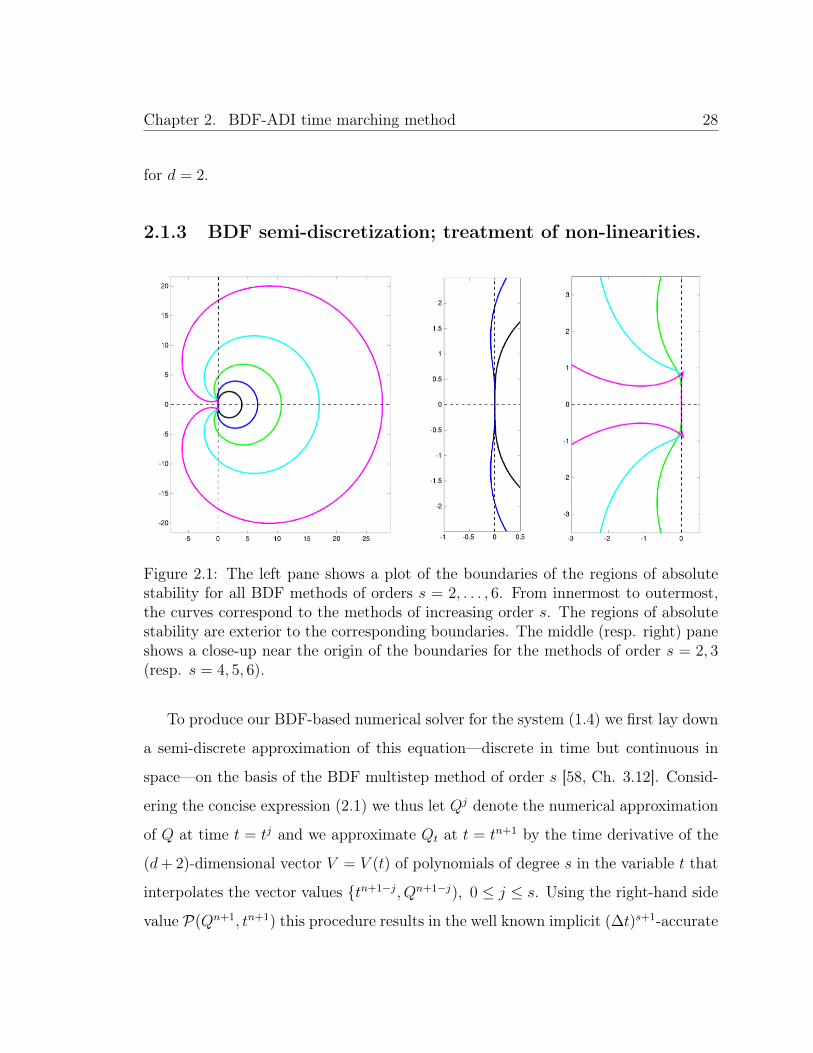
2.1 The left pane shows a plot of the boundaries of the regions of absolute
stability for all BDF methods of orders s = 2, . . . , 6. From innermost
to outermost, the curves correspond to the methods of increasing order
s. The regions of absolute stability are exterior to the corresponding
boundaries. The middle (resp. right) pane shows a close-up near the
origin of the boundaries for the methods of order s = 2, 3 (resp. s = 4, 5, 6). 28
2.2 The stability region of a hypothetical quasi-unconditionally stable method
is shown in white in the parameter space (h,∆t). The grey region is the
set of h and ∆t where the method is unstable. Notice that outside of
this window in the region a < h < Mh and ∆t > Mt, the method is sta-
ble for time steps satisfying the condition ∆t < h. Quasi-unconditional
stability does not exclude the possibility of other stability constraints
outside of the rectangular region of stability. . . . . . . . . . . . . . . . 46
List of Figures xiii
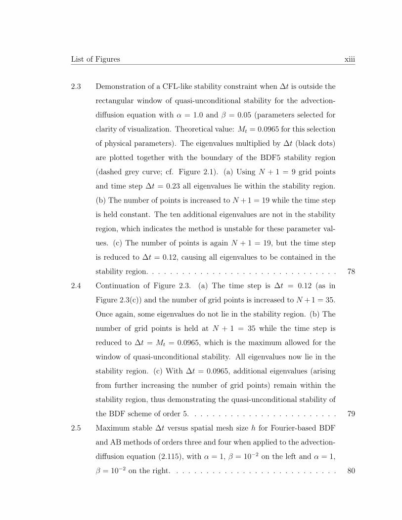
2.3 Demonstration of a CFL-like stability constraint when ∆t is outside the
rectangular window of quasi-unconditional stability for the advection-
diffusion equation with α = 1.0 and β = 0.05 (parameters selected for
clarity of visualization. Theoretical value: Mt = 0.0965 for this selection
of physical parameters). The eigenvalues multiplied by ∆t (black dots)
are plotted together with the boundary of the BDF5 stability region
(dashed grey curve; cf. Figure 2.1). (a) Using N + 1 = 9 grid points
and time step ∆t = 0.23 all eigenvalues lie within the stability region.
(b) The number of points is increased to N + 1 = 19 while the time step
is held constant. The ten additional eigenvalues are not in the stability
region, which indicates the method is unstable for these parameter val-
ues. (c) The number of points is again N + 1 = 19, but the time step
is reduced to ∆t = 0.12, causing all eigenvalues to be contained in the
stability region. . . . . . . . . . . . . . . . . . . . . . . . . . . . . . . . 78
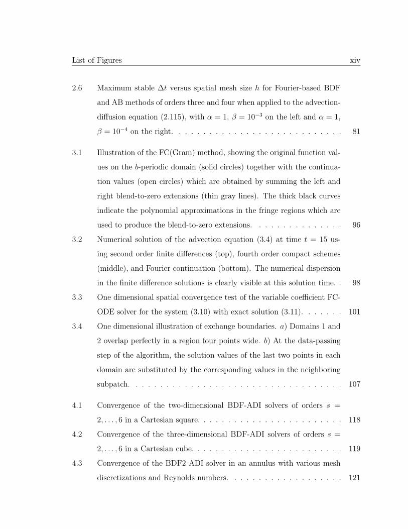
2.4 Continuation of Figure 2.3. (a) The time step is ∆t = 0.12 (as in
Figure 2.3(c)) and the number of grid points is increased to N + 1 = 35.
Once again, some eigenvalues do not lie in the stability region. (b) The
number of grid points is held at N + 1 = 35 while the time step is
reduced to ∆t = Mt = 0.0965, which is the maximum allowed for the
window of quasi-unconditional stability. All eigenvalues now lie in the
stability region. (c) With ∆t = 0.0965, additional eigenvalues (arising
from further increasing the number of grid points) remain within the
stability region, thus demonstrating the quasi-unconditional stability of
the BDF scheme of order 5. . . . . . . . . . . . . . . . . . . . . . . . . 79
2.5 Maximum stable ∆t versus spatial mesh size h for Fourier-based BDF
and AB methods of orders three and four when applied to the advection-
diffusion equation (2.115), with α = 1, β = 10−2 on the left and α = 1,
β = 10−2 on the right. . . . . . . . . . . . . . . . . . . . . . . . . . . . 80
List of Figures xiv
2.6 Maximum stable ∆t versus spatial mesh size h for Fourier-based BDF
and AB methods of orders three and four when applied to the advection-
diffusion equation (2.115), with α = 1, β = 10−3 on the left and α = 1,
β = 10−4 on the right. . . . . . . . . . . . . . . . . . . . . . . . . . . . 81
3.1 Illustration of the FC(Gram) method, showing the original function val-
ues on the b-periodic domain (solid circles) together with the continua-
tion values (open circles) which are obtained by summing the left and
right blend-to-zero extensions (thin gray lines). The thick black curves
indicate the polynomial approximations in the fringe regions which are
used to produce the blend-to-zero extensions. . . . . . . . . . . . . . . 96
3.2 Numerical solution of the advection equation (3.4) at time t = 15 us-
ing second order finite differences (top), fourth order compact schemes
(middle), and Fourier continuation (bottom). The numerical dispersion
in the finite difference solutions is clearly visible at this solution time. . 98
3.3 One dimensional spatial convergence test of the variable coefficient FC-
ODE solver for the system (3.10) with exact solution (3.11). . . . . . . 101
3.4 One dimensional illustration of exchange boundaries. a) Domains 1 and
2 overlap perfectly in a region four points wide. b) At the data-passing
step of the algorithm, the solution values of the last two points in each
domain are substituted by the corresponding values in the neighboring
subpatch. . . . . . . . . . . . . . . . . . . . . . . . . . . . . . . . . . . 107
4.1 Convergence of the two-dimensional BDF-ADI solvers of orders s =
2, . . . , 6 in a Cartesian square. . . . . . . . . . . . . . . . . . . . . . . . 118
4.2 Convergence of the three-dimensional BDF-ADI solvers of orders s =
2, . . . , 6 in a Cartesian cube. . . . . . . . . . . . . . . . . . . . . . . . . 119
4.3 Convergence of the BDF2 ADI solver in an annulus with various mesh
discretizations and Reynolds numbers. . . . . . . . . . . . . . . . . . . 121
List of Figures xv
4.4 Convergence of the BDF3 ADI solver in an annulus with various mesh
discretizations and Reynolds numbers. . . . . . . . . . . . . . . . . . . 121
4.5 Schematic set-up of unsteady flow over a bumpy plate (not to scale). . 122
4.6 Vertical velocity in two-dimensional boundary layer flow over a bumpy
plate, showing the presence of vortices and acoustic waves. From top to
bottom, the solution times for the figures are t = 9.76, 9.82, 9.88, 9.94. 124
4.7 Geometry of Taylor-Couette flow. The fluid is confined to the region
between two cylinders of radii ri and ro, and two planes separated by
a length h. The inner cylinder rotates with speed Ui, while all other
boundaries remain stationary. . . . . . . . . . . . . . . . . . . . . . . . 126
4.8 Profiles of the (a) azimuthal velocity, (b) vertical velocity, and (c) az-
imuthal component of vorticity in small-aspect-ratio Taylor-Couette flow
at Ma = 0.2 and Re = 700. The top (bottom) row has the profiles of
the two-cell (one-cell) stable mode. . . . . . . . . . . . . . . . . . . . . 127
4.9 Two close-ups of the mesh used in the numerical experiments of flow
past a cylinder. The bottom figure shows the clustering of points near
the cylinder surface to spatially resolve the boundary layer. . . . . . . 129
4.10 Temporal convergence of the solver for flow past a cylinder at time t =
1.0, with Re = 200 and Ma = 0.8. . . . . . . . . . . . . . . . . . . . . . 131
4.11 Snapshot of the vorticity in a simulation of flow past a cylinder with
Re = 200, Ma = 0.2 at time t = 82.8. . . . . . . . . . . . . . . . . . . . 133
4.12 Time evolution of streamlines in flow past a cylinder at Re = 200 and
Ma = 0.2. Darker shading of the streamline corresponds to a higher
magnitude of the velocity at that point. . . . . . . . . . . . . . . . . . 134
4.13 Temporal convergence of the three-dimensional multi-domain solver us-
ing the method of manufactured solutions at time t = 1.0, with Re = 500
and Ma = 0.8. . . . . . . . . . . . . . . . . . . . . . . . . . . . . . . . 135

List of Figures xvi
4.14 Two-dimensional slice of the mesh for flow past a sphere. The coloring
shows the sub-patch decomposition. . . . . . . . . . . . . . . . . . . . . 136
4.15 Two-dimensional x-z slice of the streamlines in a simulation of flow past
a sphere with Re = 500, Ma = 0.5 at time t = 12. Darker shades in the
streamlines indicate higher velocity magnitude. . . . . . . . . . . . . . 136
4.16 Two-dimensional x-z slice of the x-velocity (top) and density (bottom)
in flow past a sphere at Re = 500 and Ma = 0.5. . . . . . . . . . . . . . 137
4.17 Isosurfaces of the density (ρ = 0.95) in three-dimensional flow past a
sphere at times t = 64.5 (top) and t = 77.5 (bottom), showing the
apperance of hairpin vortices in the flow field. . . . . . . . . . . . . . . 138
B.1 Left: The “Yin” mesh with coarser grid spacing than used in the numer-
ical examples of flow past a sphere. Right: The composite “Yin-Yang”
mesh. . . . . . . . . . . . . . . . . . . . . . . . . . . . . . . . . . . . . 146

List of Tables xvii
List of Tables
2.1 Coefficients for BDF methods of orders s = 1, . . . , 6. . . . . . . . . . . 29
2.2 Leading order term for the real part of z(θ), the boundary locus of the
BDF method of order s stability region as θ → 0. . . . . . . . . . . . . 73
2.3 Numerical estimate of the constant mC such that for all m < mC
the parabola Γm described in Lemma 2.3 is contained in the region
of absolute stability of the BDF method of order s. By Theorem 2.4,
the order-s BDF method applied to the advection-diffusion equation
ut + αux = β uxx with Fourier collocation is stable for all ∆t < βα2mC . 74
2.4 Maximum stable ∆t for BDF-ADI methods of orders s = 2, . . . , 6 at
Reynolds number Re = 102 and Mach number 0.9 in 2D with various
numbers Ny of discretization points in the y variable. The number of
discretization points in the x direction is fixed at Nx = 12. The con-
stant Mt of quasi-unconditional stability predicted by the linear theory
(equation (2.127)) is given in the last row. . . . . . . . . . . . . . . . . 85
2.5 Same as Table 2.4 but with Reynolds number Re = 103. . . . . . . . . 85
2.6 Same as Table 2.4 but with Reynolds number Re = 104. A “Q” in the
table means there was no stable ∆t found for the given discretization.
However, using 16 points in the x direction, all entries in the table can
be filled, which is an indication of the quasi-unconditional stability of
the method. . . . . . . . . . . . . . . . . . . . . . . . . . . . . . . . . . 85
3.1 Coefficients for AB methods of orders s = 1, . . . , 4. . . . . . . . . . . . 105

List of Tables xviii
3.2 Number of seconds S needed per processor for the parallel implicit al-
gorithm to advance one million unknowns forward one time step, with
various numbers of discretization points, sub-domains, and subiterations. 115
4.1 Parameters for two-dimensional manufactured solution. The temporal
frequencies λj not in parentheses are the ones used in the convergence
tests for the methods of orders s = 2, 3, while the ones in parentheses
are those used in the order s = 4, 5, 6 tests. . . . . . . . . . . . . . . . 120
4.2 Parameters for three-dimensional manufactured solution. The temporal
frequencies λj not in parentheses are the ones used in the convergence
tests for the methods of orders s = 2, 3, while the ones in parentheses
are those used in the order s = 4, 5, 6 tests. . . . . . . . . . . . . . . . 120
Chapter 1. Introduction 1
Chapter 1
Introduction
The direct numerical simulation of fluid flow at high Reynolds numbers presents a
number of significant challenges—including the presence of structures such as bound-
ary layers, eddies, vortices and turbulence, whose accurate spatial discretization re-
quires use of fine spatial meshes. CFD (computational fluid dynamics) simulation of
such flows by means of explicit solvers is highly demanding, even on massively parallel
super computers, in view of the severe restrictions on time steps required for stability:
the time step must scale like the square of the spatial mesh size. Classical implicit
solvers do not suffer from such time step restrictions but they do require solution of
large systems of equations at each time step, and they can therefore be extremely
expensive as well.
The celebrated Beam and Warming method [6,8] provides one of the most attrac-
tive alternatives to explicit and classical implicit algorithms. Based on the alternating
direction implicit method [69] (ADI), the Beam and Warming scheme enables stable
solution of the compressible Navier-Stokes equations in times that grow only linearly
with the size of the underlying discretization, and without recourse to either nonlinear
iterative solvers or solutions of large linear systems at each time step. As discussed in
detail in the introductory portion of Chapter 2, however, previous work in the context
of the Beam and Warming method has not demonstrated accuracies beyond the first
order of temporal accuracy.

Chapter 1. Introduction 2
Nevertheless, high-order time accuracy may be crucial in the treatment of long-
time simulations or highly-inhomogeneous flows—for which the dispersion inherent in
low-order approaches would make it necessary to use inordinately small time-steps.
This thesis presents, in particular, extensions of the ADI methodology based on the
backward differentiation formulae (BDF) that exhibit orders of time accuracy between
two and six, and which are quasi-unconditionally stable, in a sense that is made
clear in Section 2.2—which essentially amounts to true unconditional stability within
certain regions in the space of discretization parameters. Further, full unconditional
stability of the second order scheme is established in the context of the convection
and parabolic linear equations. An extended discussion is presented in this thesis
which places on a solid theoretical basis the observed quasi-unconditional stability of
the s order methods with 2 ≤ s ≤ 6. In fact this thesis presents, for the first time in
the literature, high-order time-convergence curves for Navier-Stokes solvers based on
the ADI strategy.
The proposed methodology employs the BDF schemes (which are known for their
robust stability properties) together with a quasiliner-like formulation with high-
order extrapolation for nonlinear components (to produce a linear high-order time-
accurate method) and the Douglas-Gunn splitting (an ADI strategy that greatly
simplifies boundary condition treatment while retaining the order of time-accuracy of
the solver). The performance of the proposed solvers is favorable: for example, a two-
dimensional rough-surface configuration including boundary layer effects at Reynolds
number 106 and Mach number Ma = 0.8 (with a well-resolved boundary layer, run
up to a sufficiently long time that single vortices travel the entire spatial extent L
of the domain, and with spatial mesh sizes near the wall of the order of 10−5 · L)was successfully tackled in a relatively short (∼ thirty-hour) single-core run; under
similar circumstances an explicit solver would require truly prohibitive computing
times. The highest order solvers can be greatly advantageous for problems involving
long evolution times or solutions that oscillate rapidly in time; methods of lower order

Chapter 1. Introduction 3
may be more advantageous under other circumstances.
While the computational cost of the proposed BDF-ADI schemes mentioned above
grows only linearly with the size of the spatial discretization, these schemes are sig-
nificantly more expensive per time step than their explicit counterparts—such as
the explicit Fourier Continuation solver [2] (FC) we use. Thus the strategy pro-
posed in this thesis calls for use of multi-domain implicit-explicit solvers—implicit
near boundaries and other regions where fine spatial discretizations are used (which
might require extremely small time steps in an explicit solver), and explicit in re-
gions in which the size of the spatial discretization does not entail significant CFL
constraints. (The proposed multi-domain implicit-explicit schemes should not be con-
fused with similarly named IMEX methods [4] which, e.g., in an advection-diffusion
equation incorporate explicit treatment of the convective term and implicit treatment
of the diffusive term.) A brief description of the Fourier continuation methodology
and associated explicit solvers is presented below followed by an outline of the pro-
posed multi-domain implicit-explicit strategy; complete descriptions and illustrations
of these solvers follow as part of the main body of this thesis.
Most structured-grid solvers for Partial Differential Equations (PDE) are based on
the use of finite differences (FD). These methods are intuitively attractive, they can
be implemented easily, and they require limited cost per spatial discretization point.
As is well known, however, reduction of the dispersion error inherent in FD methods
requires either use of large numbers of points per wavelength, or use of higher-order
methods which typically entail higher costs and restrictive CFL constraints [2, 3,35].
Spectral methods are an attractive alternative in dealing with these challenges [10,
19, 47]. Unfortunately, polynomial spectral methods require clustering of points at
the boundaries of the domain, resulting in severe time step restrictions for explicit
methods. Classical Fourier methods, on the other hand, are only applicable to periodic
problems—otherwise they suffer from the Gibbs phenomenon and first order spatial
convergence in the interior of the domain (see, e.g., [10, Ch. 2.2]). The recently
Chapter 1. Introduction 4
introduced Fourier Continuation method (FC) provides spectral-like resolution in
non-periodic contexts without recourse to use of fine meshes; we briefly discuss this
methodology in what follows.
The FC method produces an interpolating Fourier series representation by relying
on a “periodic extension” of a given function, that closely approximates it in the
physical domain, but which is periodic on a slightly enlarged domain. In the context
of explicit algorithms, following [2, 3, 35] the FC spatial discretizations are used in
conjunction with the Adams-Bashforth (AB) method [58, Ch. 3.9] of orders two
through four. As shown in Section 3.1.2 as well as in previous references [2,3,35,64],
the resulting FC time-domain solvers (whether explicit or implicit) do give rise to
significantly improved dispersion properties, low computing costs, high accuracies
and favorable spectral asymptotics in CFL constraints—as well as parallelization
with perfect scaling. In particular, the explicit solver is significantly more accurate
than other explicit methods for similar computing times, and significantly faster than
other schemes for a given accuracy; cf. [2] and Section 3.1.2.
Unlike previous general Navier-Stokes solvers, all of the methods presented in this
thesis, including the explicit, implicit, and multi-domain solvers mentioned above,
enjoy near spatial dispersionlessness as well as higher orders of accuracy in both space
and time. Such desirable characteristics are demonstrated, in particular, by means
of implicit solutions in single domains as well as explicit and multi-domain implicit-
explicit solutions with non-trivial boundary conditions—all of which include no-slip
boundary conditions at walls, and, depending on the case under consideration, ab-
sorbing boundary conditions and inflow conditions. The proposed BDF-ADI solvers,
further, enjoy both the properties of quasi-unconditional stability, dispersionlessness,
and high-order accuracy in time. The multi-domain implicit-explicit solver, in turn, is
highly effective: results of two-dimensional flow past a cylinder and three-dimensional
flow past a sphere were produced with a significant cost savings over purely explicit
or implicit solvers. These results also represent the first demonstrations of high-order

Chapter 1. Introduction 5
time-accuracy for any Navier-Stokes solver with an implicit component (let alone
any hybrid solver) in flows of physical interest. In view of a variety of numerical
examples presented in this thesis we suggest that the accuracy levels achieved by the
proposed solvers for given spatial and temporal discretizations are unprecedented in
the literature.
In the remainder of this chapter we provide a brief account of the background
leading to the contributions in this thesis. The proposed BDF-ADI solvers are then
introduced in Chapter 2, including the concept of quasi-unconditional stability as well
as energy stability proofs for the second order schemes and spectral stability proofs
for the higher-order BDF methods. The multi-domain implicit-explicit schemes are
then presented in Chapter 3. Numerical results follow in Chapter 4, and concluding
remarks, finally, are presented in Chapter 5.
1.1 The Navier-Stokes equations for a
compressible gas
We consider the Navier-Stokes equations for a continuum fluid. Denoting by DDt
=
∂∂t
+ u · ∇ the material derivative, the Navier-Stokes system combines the equations
describing conservation of mass,
Dρ
Dt+ ρ∇ · u = 0, (1.1)
conservation of momentum,
ρDu
Dt+∇p = ∇ · σ, (1.2)
and conservation of energy,
ρDe
Dt+ p∇ · u +∇ · q = Φ, (1.3)

Chapter 1. Introduction 6
where d denotes the spatial dimensions (d = 2, 3) and where, using integer-valued
indices i, j = 1, . . . , d, u = (ui) denotes the velocity vector, and ρ, e, p, q, σ = (σij),
and Φ =∑
ij σij∂xiuj denote density, specific internal energy, pressure, heat flux,
deviatoric stress tensor, and viscous dissipation function, respectively. We narrow
our consideration to the evolution of a subsonic compressible perfect gas satisfying
the following assumptions:
1. The fluid is Newtonian, i.e., σ = µ(∇u +∇uT − 2
3(∇ · u)I
), where µ is the
viscosity and I is the identity tensor.
2. The internal energy and temperature T satisfy the thermodynamic relation
e = cvT , where cv is the specific heat at constant volume.
3. The pressure, density, and temperature are related by the equation of state for
an ideal gas p = ρRT , where R is the gas constant.
4. Fourier’s law of heat conduction q = −κ∇T holds, where κ is the thermal
conductivity.
5. For simplicity, µ and κ are functions of temperature only.
With these assumptions, choosing a characteristic length L0, velocity u0, density ρ0,
temperature T0, viscosity µ0, and heat conductivity κ0, and with a slight notational
abuse by which the non-dimensional density, velocity, and temperature ρ/ρ0, u/u0,
and T/T0 are denoted everywhere below in this thesis by the symbols ρ, u, and T ,
respectively, the non-dimensional form of the Navier-Stokes equations
ρt +∇ · (ρu) = 0 (1.4a)
ut + u · ∇u +1
γMa2
1
ρ∇(ρT ) =
1
Re
1
ρ∇ · σ (1.4b)
Tt + u · ∇T + (γ − 1)T∇ · u =γ
RePr
1
ρ∇ · (κ∇T ) +
γ(γ − 1)Ma2
Re
1
ρΦ (1.4c)

Chapter 1. Introduction 7
results, where the non-dimensional constants γ = cp/cv, Re = ρ0u0L0/µ0, Ma =
u0/√γRT0 and Pr = µ0cp/κ0 denote the ratio of specific heats, the Reynolds number,
the Mach number and the Prandtl number, respectively.
The system is completed by means of the relevant boundary conditions for a given
configuration; see, e.g., [95, Sec. 1-4] and Remark 2.1.
1.2 Implicit solvers
This section provides a brief overview of the history of implicit methods, including
considerations of stability and accuracy. Section 1.3 then discusses one of the highly
significant innovations concerning efficiency in implicit methods, namely, the alter-
nating direction implicit strategy.
1.2.1 Stability and convergence
The 1928 landmark paper by Courant, Friedrichs and Lewy [23] established that
a consistent numerical method need not converge to the exact solution of the corre-
sponding PDE, even though the numerical approximation of the problem is arbitrarily
accurate. Specifically, that paper showed that the centered difference scheme for the
wave equation cannot converge for general initial conditions unless the numerical do-
main of dependence includes the physical domain of dependence. This leads to a
linear constraint (the CFL constraint) of the form
∆t ≤ C h
for the time step ∆t and the spatial mesh size h. Note that the result is only concerned
with convergence—it does not indicate what happens to a non-converging numerical
solution of a consistent scheme. It was not until Lax’s equivalence theorem [59] in the
1950s that the connection with stability was made clear: any consistent numerical
Chapter 1. Introduction 8
method for a linear PDE converges if and only if it is stable. Certainly, while not
the name itself, the concept of stability does predate this contribution. For example,
Crank and Nicolson presented in the 1947 paper [24] the first implicit method for
PDEs based on the trapezoidal rule for time integration and showed (using a sugges-
tion by von Neumann communicated to those authors by Hartree) that the method
was stable for the heat equation for all grid spacings h and time steps ∆t, whereas the
leapfrog scheme (“Richardson’s method”) was not. However, the word “stable” in any
form does not appear in the article—what is now known as instability was termed
“rapidly increasing oscillatory error” in that early contribution.
In 1956 Dahlquist [26] established a convergence theorem for the numerical solu-
tion of ordinary differential equations (ODE) with linear multistep methods, which is
similar in spirit to Lax’s equivalence theorem (in the later contribution [27] Dahlquist
mentions, “When I wrote [that paper], I was not yet familiar with the work of Lax”).
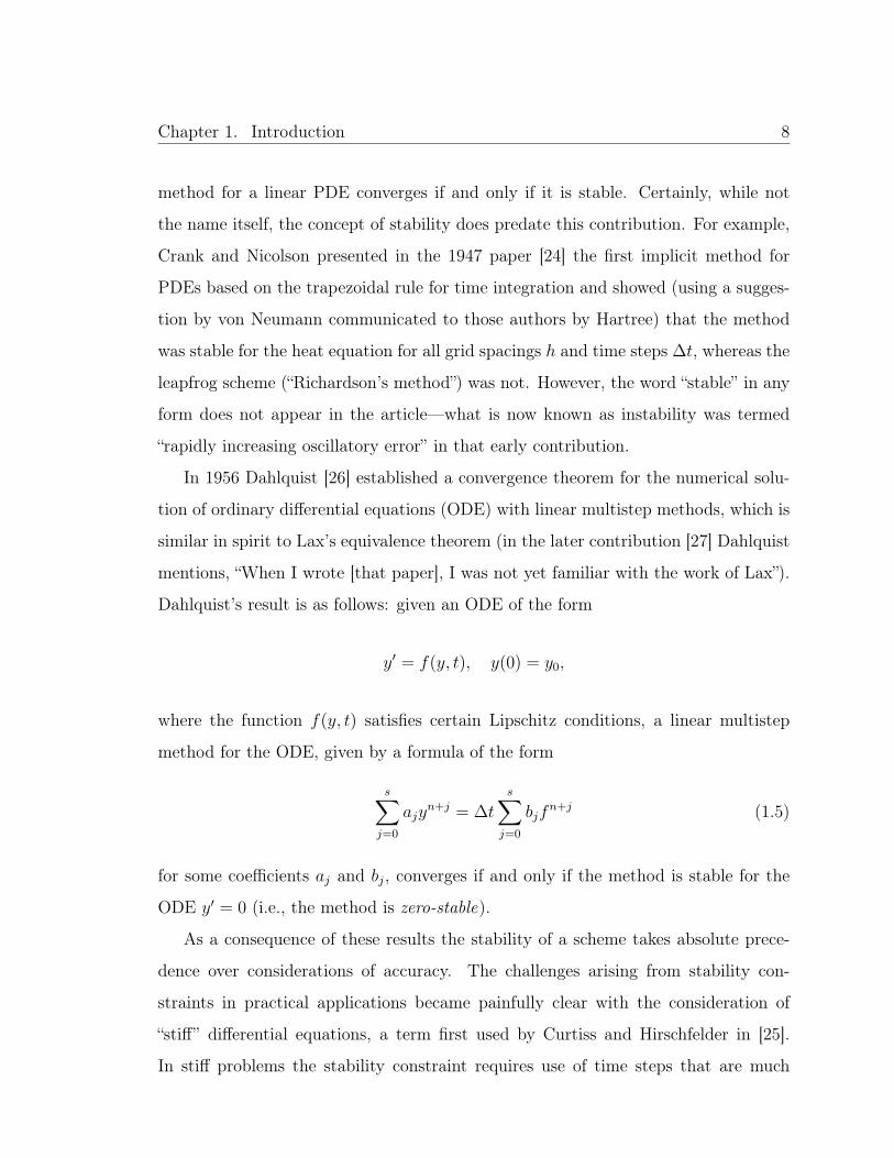
Dahlquist’s result is as follows: given an ODE of the form
y′ = f(y, t), y(0) = y0,
where the function f(y, t) satisfies certain Lipschitz conditions, a linear multistep
method for the ODE, given by a formula of the form
s∑j=0
ajyn+j = ∆t
s∑j=0
bjfn+j (1.5)
for some coefficients aj and bj, converges if and only if the method is stable for the
ODE y′ = 0 (i.e., the method is zero-stable).
As a consequence of these results the stability of a scheme takes absolute prece-
dence over considerations of accuracy. The challenges arising from stability con-
straints in practical applications became painfully clear with the consideration of
“stiff” differential equations, a term first used by Curtiss and Hirschfelder in [25].
In stiff problems the stability constraint requires use of time steps that are much

Chapter 1. Introduction 9
smaller than is otherwise necessary to resolve the time evolution of the problem. The
contribution [25] also introduces what would later become known as the backward
differentiation formulae (BDF) multistep methods as a remedy for this difficulty, and
thereby demonstrates the great value of the unconditional stability property that is
sometimes afforded by implicit methods for solutions of stiff differential equations.
Unfortunately, soon after this was established, certain severe limitations of implicit
methods in terms of temporal accuracy order were soon discovered, as discussed in
the following section.
1.2.2 Order barriers
Consider the test problem
y′(t) = λy(t) (1.6)
with λ in the complex plane C, together with an associated numerical scheme and
a given time step ∆t; as is known, any linear multistep numerical method for equa-
tion (1.6) can be expressed in terms of the quantity z = λ∆t. Letting R ⊆ C denote
the set of z = λ∆t for which the scheme is stable when applied to the above equation,
the question thus arises as to whether the scheme is “optimally” stable in this context,
that is, whether it is stable for all ∆t and for all λ for which the ODE solution is
asymptotically stable as t→ +∞. Or, equivalently, since (1.6) is asymptotically sta-
ble for for all complex values λ in the set C− of complex numbers with non-positive
real part, the question becomes whether the numerical scheme is stable for all z ∈ C−.
A method satisfying this condition is said to be A-stable. For stiff problems, which
include spectral components of the form (1.6) with large magnitude values of λ ∈ C−,
the value of A-stable methods is unquestionable.
Unfortunately, however, a fundamental limit to the accuracy order of A-stable
methods is imposed by Dahlquist’s second barrier : There are no A-stable explicit
linear multistep methods, and an (implicit) A-stable linear multistep method has ac-

Chapter 1. Introduction 10
curacy order not higher than two. There have been many attempts to “break” this
barrier by considering more general classes of multistep methods; see, e.g., the meth-
ods surveyed in [46, Chap. V.3]. There are also higher-order implicit Runge-Kutta
methods, which are not covered by Dahlquist’s theorem. Nevertheless, all such meth-
ods are subject to a more general result—the Daniel-Moore conjecture [29], proved
in [93]—which demands that higher-order A-stability comes at the cost of a certain
number of implicit solves. Specifically, any A-stable Runge-Kutta or generalized mul-
tistep method with a number s of implicit stages can have time accuracy not higher
than 2s.
Given that the use of methods that include s implicit steps can be exceedingly
expensive in the PDE context (cf. the discussion in Section 3.5.2 concerning even
a single fully-dimensional implicit solve), the alternative is to consider higher-order
methods which, while not A-stable, admit useful stability regions. In the language of
this thesis, higher-order multistep methods for the Navier-Stokes equations and other
PDEs do exist, namely quasi-unconditionally stable methods, which enjoy favorable
stability restrictions.
1.2.3 Higher order implicit methods: ODE theory
Following Dahlquist’s landmark 1963 contribution [28], a number of attempts were
made to identify and study classes of ODE solvers with favorable stability properties.
Two important concepts, namely, A(α)-stability and stiff stability, arose from these
efforts. A method is said to be A(α)-stable if the stability region R contains the
infinite “α-wedge” with vertex at the origin, given by z | arg(z) ∈ (π−α, π+α), z 6=0. A method is stiffly stable if the stability region includes the semi-infinite region
z |Rez < −a as well as the rectangle z |Rez ∈ (−a, 0), Imz ∈ (−c, c) for positivenumbers a and c. Both of these concepts are illustrated in Figure 1.1.
Unfortunately, these definitions do not provide the level of detail necessary to ad-
equately discuss the stability of PDEs such as the Navier-Stokes equations amongst

Chapter 1. Introduction 11
α
α
i c
−i c−a
Figure 1.1: A(α)-stability (left) and stiff stability (right) takes place provided theshaded area is contained in the stability region of the ODE scheme.
many others. To demonstrate this difficulty we consider the advection-diffusion equa-
tion
ut + αux = βuxx, (1.7)
which is undoubtedly the simplest model problem that could be used to understand
basic aspects of the Navier-Stokes equation. As will be shown in Section 2.4, the
eigenvalues associated with the multistep schemes for this equation are distributed in
curves that are not contained in any α-wedge with α < π/2; cf. Figure 1.1.
The concept of stiff stability, on the other hand, is not well suited for discussion
of the PDEs under consideration, since the stiff-stability regions, which are bounded
by vertical and horizontal lines, can only provide relatively crude bounds on the
parabolic-bounded eigenvalue distributions for the types of PDEs under considera-
tion. In fact, the BDF stability regions, which approximate more closely the PDE
eigenvalue distributions and which provide highly stable algorithms, are not stiffly
stable in some cases. Additionally, considerations based on stiff stability might sug-
gest that the fifth and sixth order BDF-ADI methods proposed in this work, which
are stiffly stable, ought to give rise to better stability properties in practice than the
corresponding BDF-ADI methods of orders three and four, which are not stiffly sta-
ble. This suggestion is not accurate, however. In practice, and as shown rigorously in

Chapter 1. Introduction 12
Section 2.4 for the linear advection-diffusion equation, the BDF-ADI methods of or-
ders three and four are stable for a significantly larger set of discretization parameters
than those required for stability in the methods of orders five and six.
We thus see that some of the concepts from ODE theory are not well adapted
to the context of the PDE under consideration—at least for methods of order higher
than two. (In contrast, the concept of quasi-unconditional stability introduced in
Section 2.2 does accurately capture the stability character of the BDF-ADI methods
proposed in this thesis.) Additionally, as discussed in the following section, implicit
methods with orders of temporal accuracy higher than two have received only sparse
attention in the literature. Thus the goal of the present thesis: to provide temporally
high-order Navier-Stokes solvers with unconditional stability or, failing that, with as
close a substitute as possible.
1.2.4 Higher order implicit methods: PDE applications
The state of the art for solvers of compressible flow is second order time accuracy as far
as implicit methods are concerned—and, indeed, we believe second or higher order
time-accuracy for general domains and boundary conditions has not been demon-
strated before this work. The most significant innovations for compressible fluid
solvers have concerned implementation techniques that improve efficiency (e.g., opera-
tor splittings and multigrid) or relative accuracy (e.g., Newton-like subiterations), but
such improvements do not increase the order of accuracy of the underlying method.
Perhaps the existence of Dahlquist’s second barrier may explain the widespread
use of implicit methods of orders less than or equal to two (such as backward Euler,
the trapezoidal rule and BDF2, all of which are A-stable), and the virtual absence
of implicit methods of orders higher than two—despite the near-universality of the
fourth order Runge-Kutta and Adams-Bashforth explicit counterparts. Clearly, A-
stability is not necessary for all problems—for example, any method whose stability
region contains the negative real axis (such as the BDF methods of orders two to six)

Chapter 1. Introduction 13
generally results in an unconditionally stable solver for the heat equation. A number
of important questions thus arise: Do the compressible Navier-Stokes equations in-
herently require A-stability? Are the stability constraints of all higher-order implicit
methods too stringent to be useful in the Navier-Stokes context? How close to un-
conditionally stable can a Navier-Stokes solver be whose temporal order of accuracy
is higher than two?
Unfortunately, clear answers to these questions are not available in the literature.
For example, the 2002 reference [9] compares various implicit methods for the Navier-
Stokes equations, and it states: “Practical experience indicates that large-scale engi-
neering computations are seldom stable if run with BDF4. The BDF3 scheme, with
its smaller regions of instability, is often stable but diverges for certain problems and
some spatial operators. Thus, a reasonable practitioner might use the BDF2 scheme
exclusively for large-scale computations.” However, the paper and references therein
do not investigate the stability restrictions for the higher-order BDF methods, either
theoretically or experimentally. As abundantly demonstrated in Chapter 4, however,
methods of order higher than two can have very significant advantages for certain
classes of problems, and thus, it seems useful to make available methods of a variety
of temporal orders, each one of which may be best adapted to corresponding classes
of subproblems—say, to high-frequency or to low-frequency problems; to problems
requiring solutions for small times or to problems requiring solution for long times,
etc.
The recent 2015 article [37], in turn, presents applications of the BDF scheme
up to third order of time accuracy in a finite element context for the incompress-
ible Navier-Stokes equations with turbulence modelling. This contribution does not
discuss stability restrictions for the third order solver, and, in fact, it only presents nu-
merical examples resulting from use of BDF1 and BDF2. The 2010 contribution [53],
which considers a three-dimensional advection-diffusion equation, presents various
ADI-type schemes, one of which is based on BDF3. The BDF3 stability analysis in

Chapter 1. Introduction 14
this paper, however, is restricted to the purely diffusive case.
The above examples illustrate the need for theoretical analyses and numerical
investigations of higher-order implicit methods for PDEs. A major goal of this thesis
is to make progress on both of these fronts, thus laying the groundwork for further
work in this area.
1.3 Alternating direction implicit methods
ADI methods are based on a certain operator splitting technique (in fact, the first
such technique ever introduced): they tackle PDE problems by “splitting” the relevant
underlying operator, giving rise to relatively simpler problems. In the context of a
first order system of PDEs ut = Lu, for example, operator splitting techniques use
expressions of the operator L as the sum of two or more operators, L =∑
j Lj,
which describe different characteristics of the problem. For example, the splitting
may be along the lines of slow and fast processes, small and large scales, advective
and diffusive terms, linear and nonlinear terms, or, as in the case of the ADI methods,
derivatives in each spatial dimension.
The first ADI methods were introduced in the landmark papers by Peaceman
and Rachford [69] and Douglas [30], where the schemes were used to solve the heat
equation in two dimensions,
ut = uxx + uyy.
Using a time step ∆t, and centered finite difference approximations δxx and δyy for
the second order derivatives, the Peaceman-Rachford scheme for the approximate
solution un+1 at time t = (n+ 1)∆t (for non-negative integer n) can be written as
(I −∆t δxx)u∗ = (I + ∆t δyy)u
n
(I −∆t δyy)un+1 = (I + ∆t δxx)u
∗,

Chapter 1. Introduction 15
which is formally second order accurate in space and time. Thus, the ADI split-
ting turns a large sparse system of equations into two sets of one-dimensional equa-
tions which can be solved efficiently with tridiagonal algorithms, greatly reducing
the time and memory requirements previously needed by implicit methods for multi-
dimensional PDEs.
The original papers [30, 69] generated much interest in the ADI approach, giving
rise to a number of early contributions on the subject, such as the works of Douglas
and Gunn [31,32], Fairweather and Mitchell [36], D’Yakonov [33], and Yanenko [96].
Applications to problems of fluid dynamics began with the works of Pearson [70] and
Chorin [22] for the incompressible Navier-Stokes equations. Briley and McDonald [11]
developed ADI schemes for the compressible Navier-Stokes and Euler equations.
Undoubtedly, the best-known ADI schemes for compressible fluid-dynamics are
the methods of Beam and Warming [6, 8] (also known as approximate factorization
methods (AF)), which have been successfully used for years in many compressible
Navier-Stokes solvers, e.g., [34, 41, 54, 72, 89, 90]. Besides the advantages gained by
using the ADI methodology, the Beam and Warming method also enjoys other at-
tractive properties: The time discretization is cleverly chosen in such a way that the
stability of the scheme (for certain two dimensional linear problems) follows imme-
diately from the stability for the underlying one-dimensional multistep method [94].
The method does use a linearization strategy based on first-order Taylor expansion of
certain nonlinear fluxes, which is consistent with the nominally second-order temporal
accuracies inherent in the underlying time-stepping schemes used.
Despite the success of ADI methods in general and the Beam andWarming method
in particular, challenges have remained. For example, the linearization strategy based
on the Taylor expansion mentioned above cannot be used in a higher-order method
(since higher order terms necessarily give rise to nonlinearities). The stability of
ADI methods is also difficult to analyze and, indeed, it is known [94] that the Beam
and Warming method is unstable for three dimensional linear advection equations,

Chapter 1. Introduction 16
although it is unconditionally stable in the two dimensional advection case.
Significant follow-up efforts [34, 41, 54, 72, 89, 90] have centered around the ideas
first put forth in the celebrated papers [6, 8], focusing, in particular, on enhancing
stability and restoring the (nominal) second order of accuracy inherent in the original
derivation of the method. The aforementioned follow-up algorithms incorporate vari-
ous kinds of Newton-like subiterations to reduce the errors arising from the nonlinear
terms while maintaining stability. In spite of these additions, however, the follow-up
contributions still do not demonstrate second order accuracy in time by means of
numerical examples—even though in all such cases nominally second order time step-
ping schemes are used. In contrast, these contributions do demonstrate the expected
spatial order of accuracy with a variety of numerical examples.
Perhaps the lack of numerical evidence for second-order accuracy of the Beam and
Warming method can be attributed to one of the most persistent challenges for ADI
schemes—namely, the prescription of boundary conditions for intermediate unknowns
that are stable and do not degrade the order of accuracy of the scheme (see, e.g., the
discussions in [10, Ch. 13.3] and Section 2.1.5). Although methods can sometimes
be derived for simple Dirichlet conditions (such as the boundary treatment proposed
by Beam and Warming in [7] for a scalar parabolic equation), they cannot be applied
to more general boundary conditions. Many attempts have been made to overcome
this difficulty; for example, the contribution [77] proposes a general finite difference
boundary treatment for the intermediate steps of the Beam and Warming method,
but the numerical experiments do not show second order convergence of the scheme.
Furthermore, the authors note the following:
“Beam andWarming indicated that the implicit factored method employed
in the present study should be unconditionally stable. Nevertheless, in-
stability occurs when the time step size exceeds a certain limit. Numerical
experiments performed here showed that for the conditions of the present
study, the solution was always stable when the time step size (∆t) satisfied

Chapter 1. Introduction 17
the expression
∆t < 60∆W/a0.
∆W is the smallest grid size employed in the study and a0, is the speed
of sound.”
It is unclear whether the CFL stability constraint is due to the boundary treatment
or the Beam and Warming method itself.
The boundary condition difficulties that exist for many ADI schemes can usu-
ally be traced back to a simple fact: the intermediate unknowns that arise from
the splitting are not necessarily consistent approximations of the physical solution.
A notable exception in this regard is the splitting procedure developed by Douglas
and Gunn [32]. Although not mentioned in the original papers, it was later under-
stood [12] that the Douglas-Gunn splitting (with formal order of accuracy s = 2)
yields equations for the intermediate unknowns that approximate the original PDE
to order s− 1 = 1. It follows that using the physical boundary conditions at tn+1 for
the intermediate steps preserves the order of accuracy of the method.
This thesis proposes ADI methods that address and overcome all the extant chal-
lenges to ADI-based solvers. The underlying BDF multistep method together with
BDF-like extrapolation for the nonlinear terms provides higher-order-accurate meth-
ods with quasi-unconditional stability. An extension of the Douglas-Gunn splitting to
our context guarantees the correct order of accuracy even in the presence of general
boundary conditions.
1.4 Domain decomposition
Without question, a necessary component of any solver for the challenging problems
in CFD is a method of domain decomposition. The advantages are twofold: 1) The
decomposition provides a covering of the global solution domain with simpler sub-
domains on which an approximate solution can more easily be computed and 2) a
Chapter 1. Introduction 18
domain decomposition is the natural basis for dividing the computational workload
in a parallel implementation of a numerical solver. In this section we give a brief
history of some domain decomposition strategies relevant to the one presented in this
thesis.
1.4.1 The Schwarz alternating method
The earliest contribution to domain decompositions for partial differential equations
is also the foundation of most modern domain decomposition solution strategies—
namely, the Schwarz method [75] which Schwarz developed for the same reason as
given in point 1) in the introduction to this section—to solve a problem on a complex
domain by using known solution methods on simpler ones. Here we give a brief history
of the Schwarz method; see [40] for a more detailed account.
In his Ph.D. thesis, Riemann had taken for granted the existence of solutions to
Laplace’s equation in general domains when he proved what would later be known as
the Riemann mapping theorem. When it came to his attention, he invoked what is
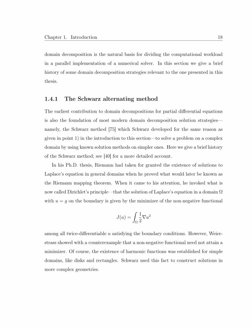
now called Dirichlet’s principle—that the solution of Laplace’s equation in a domain Ω
with u = g on the boundary is given by the minimizer of the non-negative functional
J(u) =
∫Ω
1
2∇u2
among all twice-differentiable u satisfying the boundary conditions. However, Weier-
strass showed with a counterexample that a non-negative functional need not attain a
minimizer. Of course, the existence of harmonic functions was established for simple
domains, like disks and rectangles. Schwarz used this fact to construct solutions in
more complex geometries.

Chapter 1. Introduction 19
Ω1
Ω1 ∩ Ω2 Ω2
Γ2
Γ1
∂Ω1
∂Ω2
Figure 1.2: A domain Ω given by the union of a disk Ω1 and a rectangle Ω2.
For example, consider the problem
∆u = 0 in Ω
u = g on ∂Ω
where the domain Ω is given by the union of two sub-domains Ω1 and Ω2 such that
Ω1 ∩ Ω2 6= ∅, as shown in Figure 1.2. (The disk and rectangle geometry is the
example Schwarz himself used in his paper.) Let Γ1 = ∂Ω1 ∩ Ω2 and Γ2 = ∂Ω2 ∩ Ω1.
The original Schwarz method produces the two sequences uk1 and uk2 given by the
solutions of the sub-problems∆uk+1
1 = 0 in Ω1
uk+11 = g on ∂Ω1 ∩ ∂Ω
uk+11 = uk2 on Γ1
∆uk+1
2 = 0 in Ω2
uk+12 = g on ∂Ω2 ∩ ∂Ω
uk+12 = uk+1
1 on Γ2.
(1.8)
This is also known as the alternating Schwarz method. Notice that the solution of the
second problem requires the solution of the first, so that the procedure is sequential.
Convergence of this method follows, in essence, from the maximum principle for
harmonic functions.
In the early 1990’s, Lions formally introduced the parallel Schwarz method in [63],

Chapter 1. Introduction 20
which is a modification of the original method (1.8) given by the sub-problems∆uk+1
1 = 0 in Ω1
uk+11 = g on ∂Ω1\Γ1
uk+11 = uk2 on Γ1
∆uk+1
2 = 0 in Ω2
uk+12 = g on ∂Ω2\Γ2
uk+12 = uk1 on Γ2.
(1.9)
Notice that the problems are independent, and thus form the basis for an elliptic PDE
solver in a distributed computing environment.
1.4.2 Overset/Chimera/composite grid methods
More than 20 years before the work of Lions, Volkov made the first application of
the Schwarz method to fully discrete PDEs in the method of composite meshes [92]—
indeed, Section 8 of that paper is entitled “The use of Schwarz’s alternating method
for solving a system of difference equations.” This was also the first instance of a
general class of methods which were developed around the same time and under
different names—the composite mesh method [79], the Chimera grid method [80],
and the overset grid method [13] being among the most common. In this thesis, we
will use the latter of these terms.
The overset grid method is ideally suited for solvers relying on spatial discretiza-
tions that make use of structured grids. Briefly, it involves decomposing the physical
domain into a set overlapping logical rectangles, whereby a sub-problem is solved on
each of the constituent grids. Data is communicated between these component grids
by means of interpolation.
After the introduction of the overset grid method by Volkov and subsequent de-
velopment by Starius [79], applications to CFD problems were explored by Steger,
Dougherty, and Benek [80]. The method reached a state of maturity in the 1990s with
the development of general purpose grid generation software, such as CMPGRD [21],
later to evolve into the object oriented suite Overture [13], which also includes basic

Chapter 1. Introduction 21
capabilities for solving certain PDEs on overset grids. Of course, all the early work
on overset methods was done in the context of finite differences.
More recently, the overset grid strategy has been successfully developed with the
FC methodology for the solution of the compressible Navier-Stokes equations in two
dimensions [2] and the elasticity equations in three dimensions [3]. A key development
in those contributions is the extension of the FC method to overlapping “sub-patch”
block-decompositions of larger meshes. Although the contributions [2,3] have success-
fully used the overset method in the context of explicit solvers, the goal of extending
the framework to implicit and multi-domain implicit-explicit solvers has not yet been
fully realized until now. This thesis presents the first steps toward a general frame-
work for the solution of time-domain problems using multi-domain implicit-explicit
FC solvers.
1.5 Outline of this thesis
The general outline of this thesis is as follows:
Chapter 2 introduces the BDF-ADI solver for the Navier-Stokes equations. A de-
tailed derivation is presented, which includes consideration of curvilinear coordinate
systems, treatment of nonlinear terms, the Douglas-Gunn splitting technique, and
handling of boundary conditions for the intermediate unknowns. The heart of this
chapter is the rigorous mathematical framework that is developed in support of the
BDF-ADI method. Rigorous energy proofs of unconditional stability for the Fourier-
based BDF2-ADI scheme are given for two-dimensional linear advection and parabolic
equations. The concept of quasi-unconditional stability is introduced, and we prove
that the Fourier-based BDF methods of orders s = 2, . . . , 6 for the linear advection-
diffusion equation in one, two, and three dimensions are quasi-unconditionally stable.
Finally, numerical investigations compare the stability of BDF schemes with explicit
Adams-Bashforth methods, and quasi-unconditional stability is numerically demon-
Chapter 1. Introduction 22
strated for the BDF-ADI schemes applied to the full Navier-Stokes equations in two
dimensions.
Chapter 3 presents the remaining elements necessary to complete the full multi-
domain implicit-explicit solver. The Fourier continuation methodology is presented,
together with examples showing its higher-order accuracy and dispersion relation pre-
serving property. We review the explicit time marching used in the explicit zones of
the multi-domain solver as well as the overset method and sub-patch domain decom-
position strategies. The implicit-explicit time marching method is presented, and
a simple example using the advection-diffusion equation in one dimension shows the
convergence rate of the parallel time-marching method. Numerical performance stud-
ies of the implicit multi-domain algorithm in a distributed computing environment
are also documented.
Chapter 4 showcases the BDF-ADI and multi-domain solvers with a variety of
numerical examples. The single domain BDF-ADI results use a Chebyshev collocation
spatial discretization, demonstrating the stability of the solvers even in the face of
very fine grid spacing. Numerical tests for this single-domain BDF-ADI solver include
two dimensional unsteady flow over a bumpy plate at Reynolds number 106 as well
as three dimensional wall bounded Taylor-Couette flow. Subsequently, results of the
implicit-explicit multi-domain solver in fully parallel simulations of two dimensional
flow past a cylinder and three dimensional flow past a sphere are presented. In all
cases, convergence studies are included that verify the expected temporal order of
accuracy of the proposed solvers—a first for implicit Navier-Stokes solvers; limited
emphasis is placed on the well understood [2,10,19,47] spatial high-order convergence
and dispersionlessness of the methods used.

Chapter 2. BDF-ADI time marching method 23
Chapter 2
BDF-ADI time marching method
This chapter introduces ADI solvers of higher orders of time accuracy (orders s = 2 to
6) for the compressible Navier-Stokes equations in two- and three-dimensional curvi-
linear domains. The new ADI algorithms successfully address the difficulties discussed
in Section 1.3: (i) They (provably) enjoy high orders of time-accuracy (orders two to
six) even in presence of general (and, in particular, non-periodic) boundary conditions;
and (ii) They possess remarkable stability properties, with rigorous unconditional-
stability proofs for constant coefficient hyperbolic and parabolic equations for s = 2,
and demonstrating in practice quasi-unconditional stability for 2 ≤ s ≤ 6 (Defini-
tion 2.1) and mild CFL-like constraints outside the unconditional-stability window for
s ≥ 3 (see Section 2.4.1); and (iii) They do not require use of iterative nonlinear
solvers for accuracy or stability, and they rely, instead, on a BDF-like extrapolation
technique for certain components of the nonlinear terms.
The algorithms presented in this chapter, which are based on a recently developed
ADI algorithm for the two-dimensional nonlinear Burgers system [15], are applica-
ble to general single domain curvilinear coordinate systems and are restricted in this
chapter to spectral spatial discretizations resulting from use of Fourier or polynomial
spectral expansions; an accuracy order-preserving spectral filter is used in our scheme
to ensure stability. Extensions of these algorithms to the multi-domain overset-grid
context [13] as well as to the Fourier Continuation spatial discretization [2], are pre-
Chapter 2. BDF-ADI time marching method 24
sented in subsequent chapters of this thesis. In particular, the present curvilinear
domain algorithms form the single-domain implicit component of our general multi-
domain implicit-explicit solver.
This chapter is organized as follows: Section 2.1 presents a derivation of the
BDF-ADI method in two and three dimensions, starting with a quasilinear-like for-
mulation of the equations and a transformation to general coordinates. The equation
is then discretized in time using the BDF scheme and the treatment of nonlinearities
by means of temporal extrapolation is presented. The resulting semi-discrete linear
equation is factored and split using the Douglas-Gunn procedure, and enforcement of
boundary conditions for the intermediate unknowns is discussed. After a brief review
of relevant stability ideas and introducing the concept of quasi-unconditional stabil-
ity in Section 2.2, unconditional stability is proved for the full BDF2-ADI scheme in
two dimensions applied to linear constant coefficient advection and parabolic equa-
tions in Section 2.3. Next, proofs of quasi-unconditional stability for the (non-ADI)
BDF methods applied to the constant coefficient advection-diffusion equation in one,
two, and three dimensions are presented in Section 2.4. This section also provides
qualitative analysis of the linearized Navier-Stokes equations in one spatial dimen-
sion, and numerical experiments of the full Navier-Stokes equations in two dimensions
demonstrate the quasi-unconditional stability of the solvers in practice.
2.1 Proposed BDF-ADI methodology
2.1.1 Quasilinear-like Cartesian formulation
Letting Q = (uT, T, ρ)T ∈ Rd+2 denote the full d + 2-dimensional solution vector,
clearly the equations (1.4) can be expressed in the form
Qt = P(Q, t) , x ∈ Ω , t ≥ 0, (2.1)

Chapter 2. BDF-ADI time marching method 25
where P is a vector-valued nonlinear differential operator. The operator P for the
Navier-Stokes equations (1.4) is autonomous, of course, but we include a possible t
dependence to allow for the presence of time-dependent source terms.
The derivation of the ADI method begins with a quasilinear formulation of the
equations, assuming for the moment that µ and κ are constant and neglecting the
viscous dissipation function Φ:
Qt +Mx,1(Q)∂
∂xQ+My,1(Q)
∂
∂y+M z,1(Q)
∂
∂zQ
+Mx,2(Q)∂2
∂x2Q+My,2(Q)
∂2
∂y2Q+M z,2(Q)
∂2
∂z2Q
+Mxy(Q)∂2
∂x∂yQ+Mxz(Q)
∂2
∂x∂zQ+Myz(Q)
∂2
∂y∂zQ+M0(Q)Q
= 0; (2.2)
and the corresponding equations for d = 2 are given by
Qt +Mx,1(Q)∂
∂xQ+My,1(Q)
∂
∂y+Mx,2(Q)
∂2
∂x2Q+My,2(Q)
∂2
∂y2Q
+Mxy(Q)∂2
∂x∂yQ+M0(Q)Q = 0. (2.3)
Here the variousM matrices (Mx,1, Mx,2 etc.) are matrix-valued functions of Q. The
purpose of using the quasilinear form of the equations is, upon temporal discretiza-
tion, to treat all spatial derivatives implicitly (if possible) and to approximate the
nonlinear coefficients of the derivatives explicitly in time, resulting in a linear system
of equations in Q at the current time level together with its derivatives; the details
are presented in the following sections.
The actual Navier-Stokes equations (for which µ and κ are generally functions of
T and for which Φ is non-zero) are not quasilinear, but can still be expressed in the
form (2.2) or (2.3) by allowing the matrices to incorporate some derivative terms.
For example, squared terms such as u2x are handled by including one ux term in the

Chapter 2. BDF-ADI time marching method 26
matrix Mx,1 and the second ux term in the vector ∂xQ in equation (2.3). Similarly,
the product µ(T )xuy is expanded using the chain rule and written as
µ(T )xuy = µ′(T )Txuy
=
(1
2µ′(T )Tx
)uy +
(1
2µ′(T )uy
)Tx.
The two quantities in parentheses are included in the matrices My,1 and Mx,1 re-
spectively. Thus, the implicit treatment of the product of two spatial derivatives is
symmetric. The matrices resulting from this treatment of nonlinear terms can be
found in Appendix A. Clearly, there are other ways of treating nonlinear products of
derivatives, but we chose the above for symmetry.
Remark 2.1: For notational simplicity our description of the BDF-ADI algorithms
assumes that no-slip boundary conditions of the formu
T
∣∣∣∣∣∣∂D
=
gugT
(2.4)
are prescribed, where gu and gT are given functions defined on ∂D. Certainly,
other relevant types of boundary conditions can be incorporated within the proposed
framework—Section 4.1 includes an example of unsteady boundary layer flow that
incorporates no-slip boundary conditions at a rough boundary as well as inflow and
absorbing boundary conditions.
2.1.2 Quasilinear-like curvilinear formulation
Let ξ(x, y, z), η(x, y, z), ζ(x, y, z) define a smooth mapping from the physical (Carte-
sian) domain Ω ⊂ Rd to the (ξ, η, ζ) computational domain, which we take to be the
cube D = [`1, `2]d for some real numbers `1 and `2, d = 2, 3. Using the chain rule,
the derivatives with respect to x, y, and z are expressed in terms of derivatives with
Chapter 2. BDF-ADI time marching method 27
respect to ξ, η, and ζ; see, e.g., [48]. We can then collect terms to obtain an equation
in general coordinates for Q = Q(ξ, η, ζ, t):
Qt +M ξ,1(Q)∂
∂ξQ+Mη,1(Q)
∂
∂η+M ζ,1(Q)
∂
∂ζQ
+M ξ,2(Q)∂2
∂ξ2Q+Mη,2(Q)
∂2
∂η2Q+M ζ,2(Q)
∂2
∂ζ2Q
+M ξη(Q)∂2
∂ξ∂ηQ+M ξζ(Q)
∂2
∂ξ∂ζQ+Mηζ(Q)
∂2
∂η∂ζQ+M0(Q)Q
= 0 (2.5)
for (ξ, η, ζ) ∈ D where the matrix functions M ξ,1 of Q, etc. are computed using the
Cartesian matrices and metric terms.
For d = 2 the computational domain is D = [`1, `2]2 and we have the equation
Qt +M ξ,1(Q)∂
∂ξQ+Mη,1(Q)
∂
∂η+M ξ,2(Q)
∂2
∂ξ2Q+Mη,2(Q)
∂2
∂η2Q
+M ξη(Q)∂2
∂ξ∂η+M0(Q)Q = 0. (2.6)
To simplify the presentation of boundary conditions for the ADI scheme, we de-
compose the boundary ∂D by defining
∂ξD = (ξ, η, ζ) ∈ D | ξ = `1 or `2 , (2.7a)
∂ηD = (ξ, η, ζ) ∈ D | η = `1 or `2 , (2.7b)
∂ζD = (ξ, η, ζ) ∈ D | ζ = `1 or `2 , (2.7c)
for d = 3 and
∂ξD = (ξ, η) ∈ D | ξ = `1 or `2 , (2.8a)
∂ηD = (ξ, η) ∈ D | η = `1 or `2 , (2.8b)
Chapter 2. BDF-ADI time marching method 28
for d = 2.
2.1.3 BDF semi-discretization; treatment of non-linearities.
Figure 2.1: The left pane shows a plot of the boundaries of the regions of absolutestability for all BDF methods of orders s = 2, . . . , 6. From innermost to outermost,the curves correspond to the methods of increasing order s. The regions of absolutestability are exterior to the corresponding boundaries. The middle (resp. right) paneshows a close-up near the origin of the boundaries for the methods of order s = 2, 3(resp. s = 4, 5, 6).
To produce our BDF-based numerical solver for the system (1.4) we first lay down
a semi-discrete approximation of this equation—discrete in time but continuous in
space—on the basis of the BDF multistep method of order s [58, Ch. 3.12]. Consid-
ering the concise expression (2.1) we thus let Qj denote the numerical approximation
of Q at time t = tj and we approximate Qt at t = tn+1 by the time derivative of the
(d+ 2)-dimensional vector V = V (t) of polynomials of degree s in the variable t that
interpolates the vector values tn+1−j, Qn+1−j), 0 ≤ j ≤ s. Using the right-hand side
value P(Qn+1, tn+1) this procedure results in the well known implicit (∆t)s+1-accurate

Chapter 2. BDF-ADI time marching method 29
order-s BDF formula
Qn+1 =s−1∑k=0
akQn−k + b∆tP(Qn+1, tn+1), (2.9)
where ak and b are the s-th order BDF coefficients. Table 2.1 displays the BDF
coefficients for s = 1 through 6, and Figure 2.1 shows the regions of absolute stability
in the complex plane. (BDF methods of orders greater than 6 have stability regions
that do not include a neighborhood of the origin in the region Re z < 0 and therefore
are not convergent as ∆t→ 0.)
s a0 a1 a2 a3 a4 a5 b1 1 1
2 43
−13
23
3 1811
− 911
211
611
4 4825
−3625
1625
− 325
1225
5 300137
−300137
200137
− 75137
12137
60137
6 360147
−450147
400147
−225147
72147
− 10147
60147
Table 2.1: Coefficients for BDF methods of orders s = 1, . . . , 6.
In order to express the resulting algorithm in terms of the M -matrices in equa-
tions 2.5 and 2.6, for a given (d + 2)-vector R we define the differential operators
Chapter 2. BDF-ADI time marching method 30
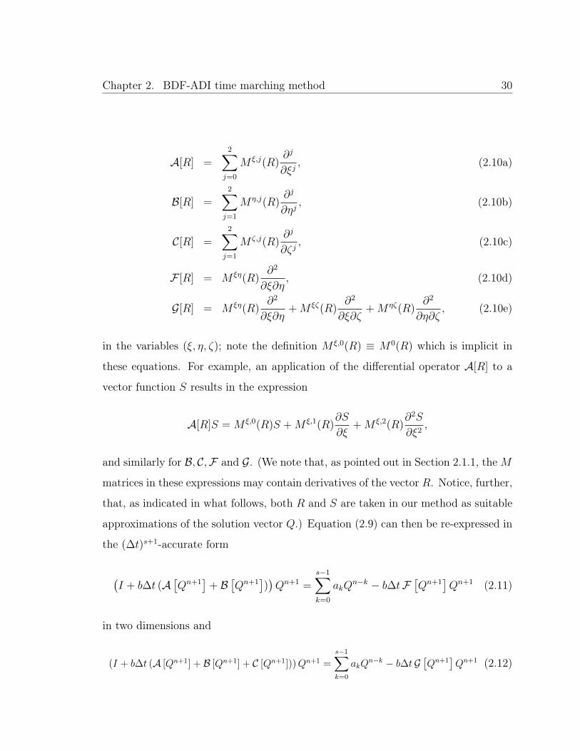
A[R] =2∑j=0
M ξ,j(R)∂j
∂ξj, (2.10a)
B[R] =2∑j=1
Mη,j(R)∂j
∂ηj, (2.10b)
C[R] =2∑j=1
M ζ,j(R)∂j
∂ζj, (2.10c)
F [R] = M ξη(R)∂2
∂ξ∂η, (2.10d)
G[R] = M ξη(R)∂2
∂ξ∂η+M ξζ(R)
∂2
∂ξ∂ζ+Mηζ(R)
∂2
∂η∂ζ, (2.10e)
in the variables (ξ, η, ζ); note the definition M ξ,0(R) ≡ M0(R) which is implicit in
these equations. For example, an application of the differential operator A[R] to a
vector function S results in the expression
A[R]S = M ξ,0(R)S +M ξ,1(R)∂S
∂ξ+M ξ,2(R)
∂2S
∂ξ2,
and similarly for B, C,F and G. (We note that, as pointed out in Section 2.1.1, theM
matrices in these expressions may contain derivatives of the vector R. Notice, further,
that, as indicated in what follows, both R and S are taken in our method as suitable
approximations of the solution vector Q.) Equation (2.9) can then be re-expressed in
the (∆t)s+1-accurate form
(I + b∆t (A
[Qn+1
]+ B
[Qn+1
]))Qn+1 =
s−1∑k=0
akQn−k − b∆tF
[Qn+1
]Qn+1 (2.11)
in two dimensions and
(I + b∆t (A [Qn+1] + B [Qn+1] + C [Qn+1]))Qn+1 =s−1∑k=0
akQn−k − b∆tG
[Qn+1
]Qn+1 (2.12)

Chapter 2. BDF-ADI time marching method 31
in three dimensions.
As mentioned in the introduction to this chapter, previous ADI-based Navier-
Stokes solvers have relied on either linearization or iterations to adequately account
for nonlinear terms. The methods proposed in this thesis, in turn, use the polynomial
extrapolations
Qn+1p ≡
p−1∑k=0
(−1)k(
p
k + 1
)Qn−k (p ≥ 1) (2.13)
to approximate the matrix-valued functions M in the operators (2.10)—which, in
particular, gives rise to high-order-accurate approximations of the full nonlinear term
at time tn+1. The formula (2.13) can be obtained by evaluating at t = tn+1 the
Lagrange interpolating polynomial
Qp(t) =
p−1∑k=0
`k(t)
`k(tn−k)Qn−k,
where tm = m∆t are equispaced points in time and where
`k(t) =∏
0≤j≤p−1j 6=k
(t− tn−j).
It follows that
Qn+1p = Qn+1 +O((∆t)p).
The extrapolated solution is used as follows: defining the variable coefficient dif-
ferential operators
As = A[Qn+1s ], Bs = B[Qn+1
s ], Cs = C[Qn+1s ], Fs = F [Qn+1
s ], Gs = G[Qn+1s ],
(2.14)
we have
AsQn+1 = A[Qn+1]Qn+1 +O((∆t)s),

Chapter 2. BDF-ADI time marching method 32
with similar expressions for the other operators in (2.14). We thus obtain the linear
equations
(I + b∆tAs + b∆tBs)Qn+1 =s−1∑k=0
akQn−k − b∆tFsQn+1 (2.15)
and
(I + b∆tAs + b∆tBs + b∆t Cs)Qn+1 =s−1∑k=0
akQn−k − b∆tGsQn+1 (2.16)
for Qn+1 in two and three dimensions, respectively. Clearly, these equations are
equivalent to the corresponding s+1-th order equations (2.11) and (2.12) respectively
up to an error of order (∆t)s+1, and thus they themselves are accurate to order s+ 1
in time. Clearly, approximations of order higher than s for the operators (2.14) (e.g.,
approximation of A, B and F in equation (2.11) by Am, Bm, and Fm, respectively,with m > s) also preserves the order of the local truncation error, but we have found
the resulting algorithms to be unstable.
2.1.4 ADI factorizations and splittings
Sections 2.1.4.1–2.1.4.4 describe our application of the Douglas-Gunn method to the
semidiscrete linear (but accurate to high order in time!) schemes (2.15) and (2.16).
Adequate treatment of the boundary conditions is a subject of great importance
that is taken up in Section 2.1.4.2 for two dimensions and Section 2.1.4.4 for three
dimensions.

Chapter 2. BDF-ADI time marching method 33
2.1.4.1 Application of the Douglas-Gunn method in two space dimensions
Adding the cross term (b∆t)2AsBsQn+1 to both sides of equation (2.15) and factoring
the resulting left-hand side exactly we obtain
(I + b∆tAs) (I + b∆tBs)Qn+1 =s−1∑k=0
akQn−k − b∆tFsQn+1 + (b∆t)2AsBsQn+1.
(2.17)
To eliminate the dependence on Qn+1 on the right-hand side of this equation we
resort once again to extrapolation: the arguments Qn+1 in the right-hand side terms
b∆tFsQn+1 and (b∆t)2AsBsQn+1 are substituted, with errors of order (∆t)s+1, by
the extrapolated values Qn+1s and Qn+1
s−1 , respectively (see equation (2.13)), and we
thus obtain the equation
(I + b∆tAs) (I + b∆tBs)Qn+1 =s−1∑k=0
akQn−k − b∆tFsQn+1
s + (b∆t)2AsBsQn+1s−1
(2.18)
whose solution only requires inversion of the operators (I + b∆tAs) and (I + b∆tBs).
Remark 2.2: Notice that, although the approximation Qn+1s−1 is accurate to order s−1
the overall accuracy order in the quantity (b∆t)2AsBsQn+1s−1 is (∆t)s+1, as needed—in
view of the (∆t)2 prefactor in this expression. While the approximation Qn+1s could
have been used while preserving the accuracy order, we have found that use of the
lower order extrapolation Qn+1s−1 is necessary to ensure stability. Similar comments
apply to the term b∆tFsQn+1s .
To complete the proposed ADI scheme an appropriate splitting of equation (2.18)
(that is, an alternating direction method for evaluation of Qn+1) must be used. The
form of the right-hand side of equation (2.18) motivates the consideration of a generic

Chapter 2. BDF-ADI time marching method 34
ADI splitting in terms of∑
kQn−k, Qn+1
s , and Qn−1s−1 :
(I + b∆tAs)Q∗ = A1
s−1∑k=0
Qn−k + A2Qn+1s + A3Q
n+1s−1 (2.19a)
(I + b∆tBs)Qn+1 = B0Q∗ +B1
s−1∑k=0
Qn−k +B2Qn+1s +B3Q
n+1s−1 (2.19b)
where Q∗ = (u∗T, T∗, ρ∗)T ∈ Rd+2 is a new intermediate unknown, and where the
various A and B terms on the right-hand sides denote operators that are as yet to
be determined. Multiplying the second equation on the left by (I + b∆tAs) and
assuming B0 and As commute, we have
(I + b∆tAs) (I + b∆tBs)Qn+1 = B0(A1
s−1∑k=0
Qn−k + A2Qn+1s + A3)
+ (I + b∆tAs) (B1
s−1∑k=0
Qn−k +B2Qn+1s +B3Q
n+1s−1 )
= (B0A1 + (I + b∆tAs)B1)s−1∑k=0
Qn−k
+ (B0A2 + (I + b∆tAs)B2)Qn+1s
+ (B0A3 + (I + b∆tAs)B3)Qn+1s−1 . (2.20)
By equating the right-hand sides of equations (2.18) and (2.20), the operators Ai and
Bi must satisfy
B0A1 + (I + b∆tAs)B1 = I, (2.21a)
B0A2 + (I + b∆tAs)B2 = −b∆tFs, (2.21b)
B0A3 + (I + b∆tAs)B3 = (b∆t)2AsBs. (2.21c)
Operators satisfying these equations exist but they are not uniquely determined.
For example, the selection B0 = I, B1 = B2 = B3 = 0 results in the classical splitting

Chapter 2. BDF-ADI time marching method 35
(I + b∆tAs)Q∗ =s−1∑k=0
akQn−k − b∆tMs Q
n+1s + b2(∆t)2AsBs Qn+1
s−1 (2.22a)
(I + b∆tBs)Qn+1 = Q∗. (2.22b)
However, as discussed in the next section, the classical splitting presents certain chal-
lenges: computable boundary conditions for the intermediate quantity Q∗ result in
reductions in the order of accuracy of the method [62]. We avoid such difficulties
by using instead the Douglas-Gunn splitting [31]. To derive it we simplify the equa-
tions (2.21) by taking B0 = b∆tAs and I, which naturally satisfy the assumption
that B0 and As commute. In the case B0 = b∆tAs we have
b∆tAs(A1 +B1) = I −B1
b∆tAs(A2 +B2) = −b∆tFs −B2
b∆tAs(A3 +B3) = (b∆t)2AsBs −B3
so that with the selections B1 = I, B2 = −b∆tFs, A1 = −B1 = −I, A2 = −B2 =
b∆tFs, and A3 = b∆tAs equations (2.21) are satisfied. These selections give rise to
the Douglas-Gunn splitting
(I + b∆tAs)Q∗ =s−1∑k=0
akQn−k − b∆tFs Qn+1
s − b∆tBs Qn+1s−1 (2.23a)
(I + b∆tBs)Qn+1 =s−1∑k=0
akQn−k − b∆tFs Qn+1
s − b∆tAsQ∗. (2.23b)
Chapter 2. BDF-ADI time marching method 36
The alternative selection B0 = I in equations (2.21) leads to the system
A1 + (I + b∆tAs)B1 = I
A2 + (I + b∆tAs)B2 = −b∆tFsA3 + (I + b∆tAs)B3 = (b∆t)2AsBs
which is satisfied provided, e.g., the additional selections B1 = B2 = 0, B3 = b∆tBs,A1 = I, A2 = −b∆tFs, and A3 = −B3 = −b∆tBs are made. The resulting ADI
splitting reads
(I + b∆tAs)Q∗ =s−1∑k=0
akQn−k − b∆tFsQn+1
s − b∆tBs Qn+1s−1 (2.24a)
(I + b∆tBs)Qn+1 = Q∗ + b∆tBs Qn+1s−1 . (2.24b)
This splitting is in fact equivalent to (2.23) (as it can be checked by subtracting
equation (2.23a) from (2.23b)). The splitting (2.24) is less expensive than (2.23)—
since 1) Equation (2.24) does not require the additional computation of the term
AsQ∗, and 2) The term b∆tBs Qn+1s−1 in (2.24) can be computed once for each full
time step and used in both ADI sweeps—and is therefore used in the two-dimensional
implementation presented in Section 2.5.
2.1.4.2 Order-preserving boundary conditions for the splitting (2.24)
Use of the two-dimensional ADI splitting (2.24) entails evaluation of solutions of sys-
tems of ODEs for the intermediate unknown Q∗ as well as the physical unknown Qn+1.
Both of these solves require use of appropriate boundary conditions. Here we show
that equations (2.24) possess the following remarkable property: imposing boundary
conditions for Q∗ which coincide with the corresponding boundary conditions for Q
at time t = tn+1 preserves the overall (∆t)s+1 truncation error otherwise implicit in
these equations.

Chapter 2. BDF-ADI time marching method 37
In view of Remark 2.1, in what follows we assume the Navier-Stokes boundary
conditions u(ξ, η, t)
T (ξ, η, t)
=
gu(ξ, η, t)
gT (ξ, η, t)
, (ξ, η) ∈ ∂D, (2.25)
for the unknown Q = (uT, T, ρ)T ∈ R2+2 (Q = Q(ξ, η, t)) at a solid-fluid interface.
Comparison of equations (2.23b) and (2.15) shows that the truncation error in (2.23b)
is a quantity of order ∆ts+1 if and only if Q∗ is an (s−1) order-accurate approximation
of Qn+1 everywhere in the domain D. But the intermediate unknown Q∗ is indeed
accurate to order s − 1 throughout D provided the boundary conditions of Q∗ are
taken to coincide with those for Q(tn+1) at the relevant interval endpoints—since,
clearly, substitution of Q∗ by Qn+1 in (2.23a) results in an equation containing an
error of order (∆t)s+1. Thus, use of boundary values of the solution at time t = tn+1
for the intermediate-time unknown Q∗ = (u∗T, T ∗, ρ∗)T, that is
u∗(ξ, η)
T ∗(ξ, η)
=
gu(ξ, η, tn+1)
gT (ξ, η, tn+1)
for ξ = `1, `2 and η ∈ [`1, `2] (2.26a)
un+1(ξ, η)
T n+1(ξ, η)
=
gu(ξ, η, tn+1)
gT (ξ, η, tn+1)
for η = `1, `2 and ξ ∈ [`1, `2], (2.26b)
maintains the overall O(∆t)s+1 truncation error in the Douglas-Gunn scheme for the
complete time step tn → tn+1. The results in Section 4.1 demonstrate the expected
order of accuracy is achieved in the case of general boundary conditions, including
cases in which time-dependent boundary conditions are specified.
Chapter 2. BDF-ADI time marching method 38
2.1.4.3 ADI factorization and splitting in three spatial dimensions
To derive the BDF-ADI method in three dimensions, we begin by factoring (2.12) to
obtain
(I + b∆tAs) (I + b∆tBs) (I + b∆t Cs)Qn+1 =s−1∑k=0
akQn−k − b∆tGsQn+1
+(b∆t)2 (AsBs +AsCs + BsCs)Qn+1
+(b∆t)3AsBsCsQn+1. (2.27)
Using polynomial extrapolations to substitute for Qn+1 on the right-hand side of the
above equation we have
(I + b∆tAs) (I + b∆tBs) (I + b∆t Cs)Qn+1 =s−1∑k=0
akQn−k − b∆tMsQ
n+1s
+(b∆t)2 (AsBs +AsCs + BsCs) Qn+1s−1
+(b∆t)3AsBsCs Qn+1s−1 , (2.28)
which is equivalent to (2.27) up to an error term of order O((∆t)s+1). Note that the
term of order (∆t)3 is extrapolated to order s − 1 rather than s − 2. Although our
experiments suggest that using a higher order extrapolation than strictly necessary
for the terms of order ∆t and (∆t)2 can give rise to instability, we have found that
the extrapolation to order s− 1 for the (∆t)3 term does not affect the stability of the
method.
A procedure similar to the one described in the two-dimensional case can be used

Chapter 2. BDF-ADI time marching method 39
to derive the Douglas-Gunn splitting
(I + b∆tAs)Q∗ =s−1∑k=0
akQn−k − b∆tMsQ
n+1s
−b∆t (Bs + Cs) Qn+1s−1 (2.29a)
(I + b∆tBs)Q∗∗ =s−1∑k=0
akQn−k − b∆tMsQ
n+1s
−b∆tAsQ∗ − b∆t CsQn+1s−1 (2.29b)
(I + b∆t Cs)Qn+1 =s−1∑k=0
akQn−k − b∆tMsQ
n+1s
−b∆tAsQ∗ − b∆tBsQ∗∗. (2.29c)
The equivalent form used in the implementation of the method is
(I + b∆tAs)Q∗ =s−1∑k=0
akQn−k − b∆tMsQ
n+1s
− b∆t (Bs + Cs) Qn+1s−1 (2.30a)
(I + b∆tBs)Q∗∗ = Q∗ + b∆tBsQn+1s−1 (2.30b)
(I + b∆t Cs)Qn+1 = Q∗∗ + b∆t CsQn+1s−1 . (2.30c)
Multiplying (2.30c) on the left by (I + b∆tAs)(I + b∆tBs) and eliminating Q∗ and
Q∗∗, it follows that (2.30) is equivalent to (2.28) up to terms on the order of the
truncation error, O((∆t)s+1).
2.1.4.4 Boundary conditions in three dimensions
As in the two-dimensional case, we show that using the boundary conditions at t =
tn+1 for the intermediate unknowns Q∗ and Q∗∗ preserves the order of accuracy of the
physical solution Qn+1. In two-dimensional space, this followed from the fact that the
ODE for Q∗ was an s−1 order accurate approximation of the unfactored PDE (2.11)
and that the ODE for Qn+1 was an s order accurate approximation of (2.11) if and
Chapter 2. BDF-ADI time marching method 40
only if Q∗ was s − 1 order accurate. By comparing the equations (2.29) to (2.12) it
follows that the ADI sweeps for Q∗, Q∗∗ and Qn+1 satisfy similar conditions – namely,
Q∗ is an s− 1 order accurate solution, Q∗∗ is s− 1 order accurate if and only if Q∗ is
s− 1 order accurate, and Qn+1 is s order accurate if and only if Q∗ and Q∗∗ are both
s− 1 order accurate. It follows that the Douglas-Gunn splitting in three dimensions
allows the use of boundary conditions at t = tn+1 when solving for the intermediate
unknowns while preserving the order of accuracy of the method.
For example, given boundary conditions of the formu
T
=
gu(ξ, η, ζ, t)
gT (ξ, η, ζ, t)
, (ξ, η, ζ) ∈ ∂D, (2.31)
the boundary conditions to be used in conjunction with the three dimensional ADI
scheme (2.30) are
u∗
T ∗
=
gu(ξ, η, ζ, tn+1)
gT (ξ, η, ζ, tn+1)
, (ξ, η, ζ) ∈ ∂ξD, (2.32a)
u∗∗
T ∗∗
=
gu(ξ, η, ζ, tn+1)
gT (ξ, η, ζ, tn+1)
, (ξ, η, ζ) ∈ ∂ηD, (2.32b)
un+1
T n+1
=
gu(ξ, η, ζ, tn+1)
gT (ξ, η, ζ, tn+1)
, (ξ, η, ζ) ∈ ∂ζD. (2.32c)
2.1.5 Discussion: enforcement of boundary conditions in pre-
vious ADI schemes
The discussion presented in this section justifies our use of the boundary values of
Q(tn+1) in the solution of the intermediate equations and it thus explains the funda-
mental advantages provided by the Douglas-Gunn splitting in our context.
As discussed in [62], substitution of physical boundary values as boundary condi-
tions for the intermediate (non-physical) variables leads to reductions in the order of

Chapter 2. BDF-ADI time marching method 41
accuracy of the overall solver unless the intermediate time steps in the ADI scheme
satisfy certain accuracy conditions. For two spatial dimensions and for a desired
overall order s of time-accuracy (i.e., the overall truncation error is O((∆t)s+1)), for
example, the desired full-step order of temporal accuracy can be guaranteed provided
the first half time step can be viewed as an (s − 1) order accurate discretization
(truncation error of order (∆t)s) throughout the domain, up to and including the
boundary, of a certain “modified” PDE of the form
Q∗t = L∗Q∗; (2.33)
see [62]. (The corresponding procedure for three dimensional problems is similar in
nature but it involves two intermediate quantities Q∗ and Q∗∗—such as those men-
tioned in Section 2.1.4.3 above. Details concerning boundary condition determination
in a particular three-dimensional example are provided in [62, Sec. 6].) The inter-
mediate solution Q∗ is then used as initial data in a corresponding modified problem
for Qn+1; the accuracy obtained for the intermediate solution Q∗ guarantees that
the complete time step (comprised of two or three intermediate time steps in two
and three dimensions, respectively) yields a solution that coincides with the unsplit
discrete solution with an error of order O((∆t)s+1).
In fact the necessary time-accurate boundary conditions for Q∗ at t = tn+1 can be
obtained [62] by means of a Taylor expansion of Q∗ at t = tn: applying the Taylor
series procedure (whereby the PDE is differentiated to obtain subsequent terms in
a Taylor series expansion of the solution) to equation (2.33) with initial conditions
Q∗ = Qn at t = tn, a truncated power series solution of the appropriate order of
accuracy is constructed which is then evaluated at t = tn+1 to produce the desired
boundary condition for Q∗ at that time. This prescription ensures that the errors
in boundary values for intermediate variables Q∗ are quantities of the appropriate
order of time accuracy and, thus, that agreement between the full-step split and

Chapter 2. BDF-ADI time marching method 42
unsplit discrete schemes to order (∆t)s+1 takes place throughout the domain, up to
and including the domain boundary.
The order-s boundary-condition prescriptions provided in [62] are expressed in
terms of certain spatial derivatives of the numerical solution Qn: each subsequent
order of time accuracy requires an additional term in the formal power series solu-
tion, and, thus, in view of the Taylor series method used, it requires several spatial
derivatives of the numerical solution Qn at the boundary. For the heat equation and
the Navier-Stokes equation, for example, two additional spatial derivatives of the nu-
merical solution at the boundary are in principle necessary for each additional order
of time accuracy. But, as pointed out in [62], the original PDE can be used to express
such derivatives in terms of derivatives with respect to time together with a derivative
of the highest order along the boundary (which do not present difficulties as they can
be obtained from the boundary conditions) as well as numerical derivatives of the
discrete solution Qn of orders lower than the maximum order of spatial differentia-
tion in the original PDE. In some cases, simplifications can be made such that the
resulting expression for Q∗ at the boundary is only in terms of the given boundary
data for Q at t = tn and tn+1. For example, in the context of the split (2.22), using
equation (2.22b), the boundary condition
Q∗ = (I + b∆tB)(Q(tn+1)−Qn ), (ξ, η) ∈ ∂ξD (2.34)
can be used when Dirichlet data for Q is specified. For the Navier-Stokes equations,
however, evaluation of the boundary condition for Q∗ requires differentiation of the
numerical solution at the boundary of orders as high as the desired order s of temporal
accuracy—which could give rise to accuracy losses and, owing to its dependence on
solution values at time t = tn, it would give rise to CFL-type constraints in otherwise
unconditionally stable implicit solvers.
The Douglas-Gunn scheme is exceptional in that a modified PDE can always be

Chapter 2. BDF-ADI time marching method 43
obtained yielding boundary values at t = tn+1 which can be obtained simply and
without any recourse to differentiation: the t = tn+1 boundary condition implied by
this modified PDE for the intermediate variables exactly coincides with the physical
boundary conditions at time t = tn+1—for any time accuracy order used. In detail, in
the Douglas-Gunn scheme the intermediate relation (2.23a) is an order s−1 accurate
approximation of the full PDE (1.4), with truncation error of order (∆t)s. Note that
since Q∗ is multiplied by ∆t in equation (2.23b) this O((∆t)s) additional error does
not change the temporal order of accuracy (∆t)s of the overall scheme carried up to
O(1) time. Thus, the Taylor expansion procedure applied at a boundary point and at
time tn provides solutions at time tn+1 which, in view of the smoothness of solutions
and prescribed initial boundary data for the original equation (2.1), must satisfy the
boundary conditions imposed on the exact solution Q up to an error of the relevant
order (∆t)s.
Remark 2.3: It is interesting to note that the boundary conditions for the intermedi-
ate variables Q∗ in the Douglas-Gunn scheme necessarily coincide with those imposed
on the exact solution up to a difference of order (∆t)s—for any type of boundary
conditions imposed on Qn+1, whether of Dirichlet type, Neumann type, Robin type,
etc. Indeed, the exact physical solution Q is a solution of the modified PDE for Q∗
with an error of the order (∆t)s for tn ≤ t ≤ tn+1 = tn + ∆t and, thus, the full
Taylor series in space and time must coincide, up to order (∆t)s and for all orders
in the spatial variables not only at the boundary but throughout the physical domain.
Additionally, since they do not entail boundary or solution values at time t = tn, the
Douglas-Gunn boundary conditions do not induce any CFL-type constraints.

Chapter 2. BDF-ADI time marching method 44
2.2 Stability and quasi-unconditional stability
proofs: discussion
Clearly, an implicit solver such as the one presented in this thesis is more expensive per
point per time step than an explicit solver. However, using an implicit solver makes
sense when the time step restrictions imposed by the mesh spacing h are too severe
for the explicit solver—assuming the implicit solver has favorable stability properties,
or course. In this section we apply the relevant stability concepts from ODE and
PDE theory, and we introduce the new concept of quasi-unconditional stability.
There are many definitions of stability to be found in the literature. Some authors
(e.g., [45, 61]) define stability as the uniform boundedness for small enough mesh
sizes h and time steps ∆t of the solution operators arising from spatial and temporal
discretization of the PDE. In this chapter we will instead define stability as the
boundedness of solutions in terms of their initial data (see, e.g., [81]): using a norm
| · | which quantifies the size of the solution at some fixed point t in time, we say
that a scheme is stable within some region Λ ⊂ (h,∆t) : h > 0, ∆t > 0 of
the discretization-parameter space if and only if for any final time T ∈ R and all
(h,∆t) ∈ Λ the estimate
|Qn| ≤ CT
J∑j=0
|Qj| for all 0 ≤ n∆t ≤ T (2.35)
holds for some integer J , for some constant CT which depends only on T (see [81]).
A method is unconditionally stable for a given PDE problem if such a constant CT
can be found for all discretization parameters (h,∆t) ∈ (0,∞)× (0,∞).
The region of absolute stability R of an ODE scheme is the set of complex numbers
z = λ∆t such that the solution of the ODE y′(t) = λ y(t) is stable with time step ∆t.
Ideally, one might hope for a method to be stable when the exact solution is stable—
i.e., the method is stable for all λ with non-positive real part, regardless of ∆t. A
Chapter 2. BDF-ADI time marching method 45
scheme with this property is said to be A-stable. In fact, the first- and second order
BDF ODE solvers are A-stable, and thus may lead to unconditionally stable methods
for linear PDEs. As is well known, however, implicit linear multistep methods of
order greater than two are not A-stable (Dahlquist’s second barrier [28]). It follows
that the BDF schemes of order s ≥ 3 are not A-stable; nevertheless, we will see that
for some problems they may enjoy the property of quasi-unconditional stability—a
concept that we define below.
Definition 2.1: Let Ωh be a family of spatial discretizations of a domain Ω controlled
by a mesh-size parameter h and let ∆t be a temporal step size. A numerical method
for the solution of the PDE Qt = P Q in Ω is said to be quasi-unconditionally
stable if there exist positive constants Mh and Mt such that the method is stable for
all h < Mh and all ∆t < Mt.
Clearly, quasi-unconditional stability implies that for small enough ∆t, the method
is stable for arbitrarily fine spatial discretizations. Note that, outside of the region
of quasi-unconditional stability, there could be other stability conditions. For exam-
ple, Figure 2.2 illustrates the concept of quasi-unconditional stability in the param-
eter space (h,∆t) in a case where a CFL type constraint exists outside the window
(0,Mh)× (0,Mt).
In lieu of a full stability analysis for the main problem under consideration (the
fully nonlinear compressible Navier-Stokes equations, for which stability analyses are
not available for any of the various extant algorithms), in support of the stability
behavior observed in our numerical experiments we present rigorous stability results
for simpler related problems. In particular, in Section 2.3 we establish the uncondi-
tional stability of the Fourier-based BDF2-ADI scheme for linear constant coefficient
hyperbolic and parabolic equations in two spatial dimensions. In Section 2.4 we prove
quasi-unconditional stability of Fourier-spectral BDF methods (2 ≤ s ≤ 6, without
ADI) for the advection-diffusion equation in one- and two-dimensional space using

Chapter 2. BDF-ADI time marching method 46
∆t
h0
Mt
Mha
Figure 2.2: The stability region of a hypothetical quasi-unconditionally stable methodis shown in white in the parameter space (h,∆t). The grey region is the set of h and∆t where the method is unstable. Notice that outside of this window in the regiona < h < Mh and ∆t > Mt, the method is stable for time steps satisfying thecondition ∆t < h. Quasi-unconditional stability does not exclude the possibility ofother stability constraints outside of the rectangular region of stability.
von Neumann stability analysis, together with numerical results that demonstrate
quasi-unconditional stability for the full compressible Navier-Stokes equations.
Remark 2.4: In general, the stability of a PDE solver can be ensured provided rele-
vant discrete operators are power bounded [87]. The von Neumann criterion provides a
necessary but not sufficient condition for the power-boundedness of solution operators.
If the discrete operators are non-normal, then stability analysis requires application
of the Kreiss matrix theorem [45, p. 177]. In particular, it is known [87,88] that cer-
tain discretizations and numerical boundary conditions can give rise to non-normal
families of solution operators that are not power-bounded (and unstable) even though
the underlying problem is linear with constant coefficients and all eigenvalues are in-
side the unit disk. (An operator P with adjoint P ∗ is normal if P ∗P = PP ∗.) In
our Fourier-spectral context, however, all operators are normal (which follows from
the fact that the first derivative operators are skew-Hermitian, the second derivative

Chapter 2. BDF-ADI time marching method 47
operators are Hermitian, and all derivative operators commute) and consequently the
von Neumann criterion is both necessary and sufficient (cf. [47, p. 189]).
2.3 Stability estimates: linear case, Fourier-BDF2
We use the energy method to prove the unconditional stability of the BDF2-ADI
scheme for constant coefficient hyperbolic and parabolic equations with periodic
boundary conditions and a Fourier collocation spatial approximation. The proofs
in both the parabolic and hyperbolic case rely on the facts that certain boundary
terms that arise from integration by parts vanish and that the discrete trapezoidal
quadrature based on the underlying spatial discretization is exact for all the integra-
tions used. Therefore, the proof for the parabolic equation is essentially the same
if a Legendre collocation spatial approximation is used with homogeneous bound-
ary conditions. However, the same generalization cannot be made for the hyperbolic
problem because not all boundary terms from integration by parts cancel (see [43] for
a discussion of spectral method stability proofs for hyperbolic problems).
2.3.1 Preliminary definitions
We consider the domain
Ω = [0, 2π)× [0, 2π) (2.36)
and discretize Ω on the basis of an odd number N+1 of discretization points (N even,
for definiteness) in both x and y directions (xj = 2πj/(N + 1) and yk = 2πk/(N + 1),
0 ≤ j, k ≤ N), which defines the grid
(xj, yk) : 0 ≤ j, k ≤ N. (2.37)
(Our restriction to even values of N is made so as to avoid having to change the limits
of the Fourier series (2.40). Similarly, our requirement that equal numbers of points
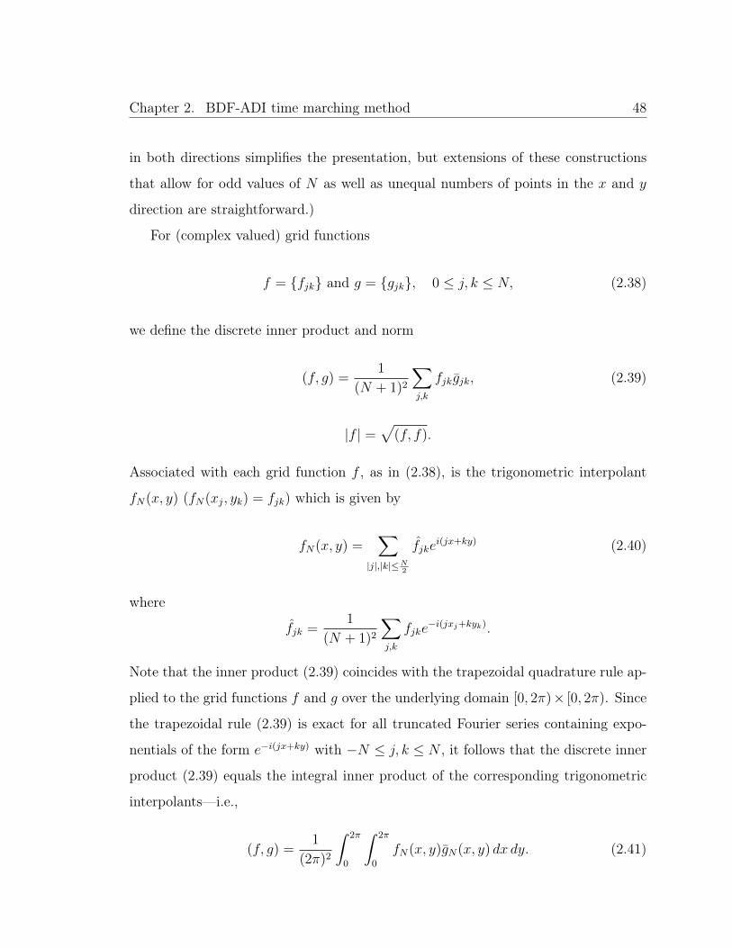
Chapter 2. BDF-ADI time marching method 48
in both directions simplifies the presentation, but extensions of these constructions
that allow for odd values of N as well as unequal numbers of points in the x and y
direction are straightforward.)
For (complex valued) grid functions
f = fjk and g = gjk, 0 ≤ j, k ≤ N, (2.38)
we define the discrete inner product and norm
(f, g) =1
(N + 1)2
∑j,k
fjkgjk, (2.39)
|f | =√
(f, f).
Associated with each grid function f , as in (2.38), is the trigonometric interpolant
fN(x, y) (fN(xj, yk) = fjk) which is given by
fN(x, y) =∑
|j|,|k|≤N2
fjkei(jx+ky) (2.40)
where
fjk =1
(N + 1)2
∑j,k
fjke−i(jxj+kyk).
Note that the inner product (2.39) coincides with the trapezoidal quadrature rule ap-
plied to the grid functions f and g over the underlying domain [0, 2π)× [0, 2π). Since
the trapezoidal rule (2.39) is exact for all truncated Fourier series containing expo-
nentials of the form e−i(jx+ky) with −N ≤ j, k ≤ N , it follows that the discrete inner
product (2.39) equals the integral inner product of the corresponding trigonometric
interpolants—i.e.,
(f, g) =1
(2π)2
∫ 2π
0
∫ 2π
0
fN(x, y)gN(x, y) dx dy. (2.41)

Chapter 2. BDF-ADI time marching method 49
To discretize solutions of time-domain PDEs, we use time sequences of grid func-
tions u = un : n ≥ 0, where, for each n, un = unjk is a grid function such as those
displayed in equation (2.38). For such time series the scalar product (2.39) at fixed
n can be used to produce a time series of scalar products: the inner product of two
time series of grid functions u = un and v = vn is thus a time series of complex
numbers:
(u, v) = (un, vn) : n ≥ 0.
2.3.2 Discrete spatial and temporal operators
The discretization of PDE differential operators proceeds by defining spatial and tem-
poral differentiation operators that act on grid functions and time-series, respectively.
We consider spatial differentiation first: the Fourier x-derivative operator δx ap-
plied to a grid function f , for example, is defined as the grid function δxf whose jk
value equals the value of the derivative of the interpolant fN at the point (xj, yk):
(δxf)jk =∂
∂xfN(xj, yk). (2.42)
The operators δxx, δy, δyy, δxy = δxδy = δyδx etc. are defined similarly.
Using the exactness relation (2.41) and integration by parts together with the
periodicity of the domain, it follows that the first derivative operators δx and δy are
skew-Hermitian and the second derivative operators δxx, δyy are Hermitian:
(δxf, g) = −(f, δxg), (δyf, g) = −(f, δyg), (2.43a)
(δxxf, g) = (f, δxxg), (δyyf, g) = (f, δyyg). (2.43b)
Certain temporal differentiation and extrapolation operators we use, in turn, pro-
duce new time series from a given numerical time series or time series of grid functions.
These operators include the regular first and second order finite difference operators

Chapter 2. BDF-ADI time marching method 50
D and D2, the three-point backward difference operator D that is inherent in the
BDF2 algorithm, as well as the second order accurate extrapolation operator “∼”:
(Du)n = un − un−1 n ≥ 1, (2.44)
(D2u)n = (Du)n − (Du)n−1 = un − 2un−1 + un−2 n ≥ 2, (2.45)
(Du)n =3
2un − 2un−1 +
1
2un−2 n ≥ 2, (2.46)
un+1 = 2un − un−1 n ≥ 1. (2.47)
Note that the members of the time series Du can also be expressed as follows
(Du)n = D
(un +
1
2(Du)n
)(2.48)
=1
2((Du)n + (Du)n+1) (2.49)
=3
2(Du)n − 1
2(Du)n−1. (2.50)
In what follows we will make frequent use of the finite difference product rule for
two time series u and v:
uDv = D(uv)− v Du+ (Du) (Dv). (2.51)
One immediate consequence of (2.51), which will also prove useful, concerns the real
part of scalar products with a given operator P that is self-adjoint with respect to
the discrete inner product (2.39) and which commutes with D:
<(Du, P u) =1
2D(u, P u) +
1
2(Du, P Du). (2.52)

Chapter 2. BDF-ADI time marching method 51
This expression follows easily from the relations
(Du, P u) = D(u, P u)− (u,DP u) + (Du,DP u)
= D(u, P u)− (P u,Du) + (Du, P Du)
= D(u, P u)− (Du, P u) + (Du, P Du).
2.3.3 Fourier-based BDF2-ADI stability: hyperbolic equation
This section establishes the unconditional stability of the BDF2-ADI method for the
constant-coefficient convection equation
Ut + αUx + βUy = 0 (2.53)
in the domain (2.36) with real constants α and β, subject to periodic boundary
conditions. The factored form (2.18) of the BDF2-ADI scheme for the Navier-Stokes
equations can easily be specialized to the present case. Indeed, using the Fourier
collocation approximation described in the previous two sections, setting As = αδx
and Bs = βδy (cf. equation (2.42)), letting u denote the discrete approximation of the
solution U (that is, letting Q = u, s = 2 in (2.18)), and noting that the extrapolated
term is given by Qn+11 = un, the factored form (2.18) for the BDF2-ADI method
applied to the convection equation (2.53) reads
(I + b∆tαδx)(I + b∆tβδy)un+1 = a0u
n + a1un−1 + αβ(b∆t)2δxδyu
n. (2.54)
Before proceeding to our stability result we derive a more convenient (equivalent)
form for equation (2.54): using the numerical values a0 = 4/3, a1 = −1/3, and
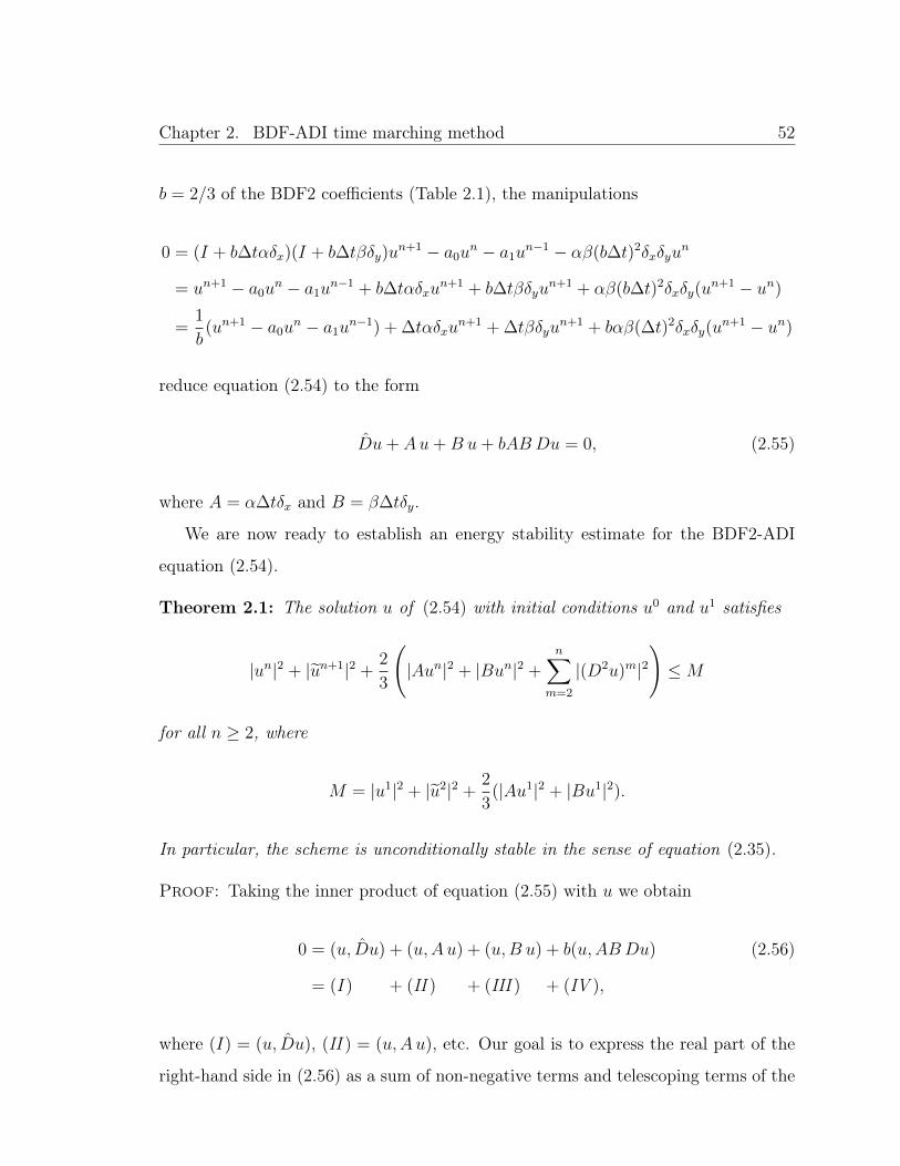
Chapter 2. BDF-ADI time marching method 52
b = 2/3 of the BDF2 coefficients (Table 2.1), the manipulations
0 = (I + b∆tαδx)(I + b∆tβδy)un+1 − a0u
n − a1un−1 − αβ(b∆t)2δxδyu
n
= un+1 − a0un − a1u
n−1 + b∆tαδxun+1 + b∆tβδyu
n+1 + αβ(b∆t)2δxδy(un+1 − un)
=1
b(un+1 − a0u
n − a1un−1) + ∆tαδxu
n+1 + ∆tβδyun+1 + bαβ(∆t)2δxδy(u
n+1 − un)
reduce equation (2.54) to the form
Du+ Au+B u+ bABDu = 0, (2.55)
where A = α∆tδx and B = β∆tδy.
We are now ready to establish an energy stability estimate for the BDF2-ADI
equation (2.54).
Theorem 2.1: The solution u of (2.54) with initial conditions u0 and u1 satisfies
|un|2 + |un+1|2 +2
3
(|Aun|2 + |Bun|2 +
n∑m=2
|(D2u)m|2)≤M
for all n ≥ 2, where
M = |u1|2 + |u2|2 +2
3(|Au1|2 + |Bu1|2).
In particular, the scheme is unconditionally stable in the sense of equation (2.35).
Proof: Taking the inner product of equation (2.55) with u we obtain
0 = (u, Du) + (u,Au) + (u,B u) + b(u,ABDu) (2.56)
= (I ) + (II ) + (III ) + (IV ),
where (I) = (u, Du), (II ) = (u,Au), etc. Our goal is to express the real part of the
right-hand side in (2.56) as a sum of non-negative terms and telescoping terms of the

Chapter 2. BDF-ADI time marching method 53
form Df for some non-negative numerical time series f . To that end, we consider the
terms (I) through (IV ) in turn.
(I ): Using the expression (2.49) for Du we obtain
(I) =1
2(u,Du) +
1
2(u,Dw), (2.57)
where w denotes the time series obtained by shifting u forwards by one time step:
w = wn = un+1 : n ≥ 1. (2.58)
To re-express (2.57) we first note that for any two grid functions a and b we have the
relation
|a− b|2 = |a|2 + |b|2 − 2<(a, b)
=⇒ <(a, b) =1
2(|a|2 + |b|2 − |a− b|2).
Therefore, for any time series g we have
<(u,Dg)n = <(un, gn)−<(un, gn−1)
=1
2(|un|2 + |gn|2 − |un − gn|2)− 1
2(|un|2 + |gn−1|2 − |un − gn−1|2)
=1
2(D|gn|2 − |un − gn|2 + |un − gn−1|2). (2.59)
Letting g = u and g = w in (2.59) we obtain
<(u,Du) =1
2(D|u|2 + |Du|2) (2.60)
and
<(u,Dw) =1
2(D|w|2 − |Du|2 + |D2u|2). (2.61)

Chapter 2. BDF-ADI time marching method 54
Replacing (2.60) and (2.61) in (2.57) we obtain
<(I ) =1
4D(|u|2 + |w|2) +
1
4|D2u|2. (2.62)
Notice that this equation expresses <(I ) as the sum of a telescoping term and a
positive term, as desired.
(II ) and (III): The operator A is clearly skew-Hermitian since δx is. Therefore
(II ) = (u,Au) = −(Au, u) = −(u,Au)
=⇒ <(II ) = 0. (2.63)
The relation
<(III ) = <(u,Bu) = 0 (2.64)
follows similarly, of course.
(IV ): Lemma 2.1 below tells us that
<(u,ABDu) ≥ 1
4D(|Au|2 + |Bu|2
)− 1
8|D2u|2. (2.65)
Combining equations (2.62), (2.63), (2.64), and (2.65) into equation (2.56) (recall-
ing b = 2/3) and taking the real part we obtain
0 ≥ 1
4D(|u|2 + |w|2
)+
1
6
(|Au|2 + |Bu|2 + |D2u|2
), (2.66)
which is the sum of a telescoping term and a non-negative term. Multiplying by
the number four and summing the elements of the above numerical time series from
m = 2 to n proves the result.
The following lemma concerns the bound (2.65) used in Theorem 2.1.
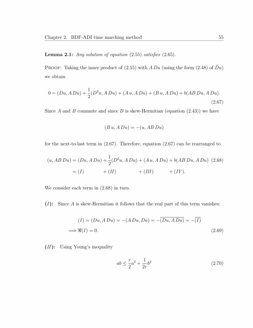
Chapter 2. BDF-ADI time marching method 55
Lemma 2.1: Any solution of equation (2.55) satisfies (2.65).
Proof: Taking the inner product of (2.55) with ADu (using the form (2.48) of Du)
we obtain
0 = (Du,ADu) +1
2(D2u,ADu) + (Au,ADu) + (B u,ADu) + b(ABDu,ADu).
(2.67)
Since A and B commute and since B is skew-Hermitian (equation (2.43)) we have
(B u,ADu) = −(u,ABDu)
for the next-to-last term in (2.67). Therefore, equation (2.67) can be rearranged to
(u,ABDu) = (Du,ADu) +1
2(D2u,ADu) + (Au,ADu) + b(ABDu,ADu) (2.68)
= (I) + (II ) + (III ) + (IV ).
We consider each term in (2.68) in turn.
(I): Since A is skew-Hermitian it follows that the real part of this term vanishes:
(I ) = (Du,ADu) = −(ADu,Du) = −(Du,ADu) = −(I )
=⇒ <(I ) = 0. (2.69)
(II ): Using Young’s inequality
ab ≤ r
2a2 +
1
2rb2 (2.70)

Chapter 2. BDF-ADI time marching method 56
(which, as is easily checked, is valid for all real numbers a and b and for all r > 0)
together with the Cauchy-Schwarz inequality we obtain
<(II ) =1
2<(D2u,ADu)
≥ −1
2|(D2u,ADu)|
≥ −1
2|D2u| |ADu|
≥ −1
2(1
4|D2u|2 + |ADu|2)
= −1
8|D2u|2 − 1
2|ADu|2. (2.71)
(III ): By the finite-difference product rule (2.51) we obtain
(III ) = (Au,D(Au))
= D(Au,Au)− (DAu,Au) + (DAu,DAu)
= D|Au|2 − (III) + |ADu|2
=⇒ <(III) =1
2D|Au|2 +
1
2|ADu|2. (2.72)
(IV ): Again using the fact that B is skew-Hermitian and commutes with A it follows
that
(IV ) = b(BADu,ADu) = −b(ADu,BADu) = −(IV )
=⇒ <(IV ) = 0. (2.73)
Combining the real parts of equations (2.68), (2.69), (2.71), (2.72) and (2.73) we
obtain
<(u,ABDu) ≥ 1
2D|Au|2 − 1
8|D2u|2. (2.74)
An analogous result can be obtained by taking the inner product of equation (2.55)
with BDu instead of ADu and following the same steps used to arrive at equa-

Chapter 2. BDF-ADI time marching method 57
tion (2.74). The result is
<(u,ABDu) ≥ 1
2D|Bu|2 − 1
8|D2u|2. (2.75)
The lemma now follows by averaging equations (2.74) and (2.75).
2.3.4 Fourier-based BDF2-ADI stability: parabolic equation
This section establishes the unconditional stability of the BDF2-ADI method for the
constant-coefficient parabolic equation
Ut = αUxx + β Uyy + γ Uxy. (2.76)
Notice the inclusion of the mixed derivative term, which is treated explicitly us-
ing temporal extrapolation in the BDF-ADI algorithm. Theorem 2.2 in this section
proves, in particular, that extrapolation of the mixed derivative does not compromise
the unconditional stability of the method.
The parabolicity conditions α > 0, β > 0 and
γ2 ≤ 4αβ, (2.77)
which are assumed throughout this section, ensure that
∫ 2π
0
∫ 2π
0
f (α fxx + β fyy + γ fxy) dx dy ≤ 0 (2.78)
for any twice continuously differentiable bi-periodic function f defined in the do-
main (2.36)—as can be established easily by integration by parts and completion of
the square in the sum α(fx)2 + γfxfy together with some simple manipulations. In
preparation for the stability proof that is put forth below in this section, in what
follows we present a few preliminaries concerning the BDF2-ADI algorithm for equa-

Chapter 2. BDF-ADI time marching method 58
tion (2.76).
We first note that a calculation similar to that leading to equation (2.55) shows
that the Fourier-based BDF2-ADI scheme for (2.76) can be expressed in the form
Du−∆t(α δxx + β δyyu+ γ δxδy)u+ ∆t γ δxδyD2u+ b(∆t)2αβ δxxδyyDu = 0. (2.79)
Letting
A = −∆t α δxx,
B = −∆t β δyy,
F = −∆t γ δxδy,
L = A+B + F,
equation (2.79) becomes
Du+ Lu− F D2u+ bABDu = 0. (2.80)
Note that the operators A and B above do not coincide with the corresponding A
and B operators in Section 2.3.3.
In view of the exactness relation (2.41) together with the Fourier differentiation
operators (cf. (2.42)), it follows that A, B, AB and L are positive semidefinite oper-
ators. Indeed, in view of equation (2.78), for example, we have
(u, L u) = − ∆t
(2π)2
∫ 2π
0
∫ 2π
0
uN (α(uN)xx + β(uN)yy + γ(uN)xy) dx dy
≥ 0; (2.81)
similar relations for A, B and AB follow directly by integration by parts.
Finally we present yet another consequence of the parabolicity condition (2.77)
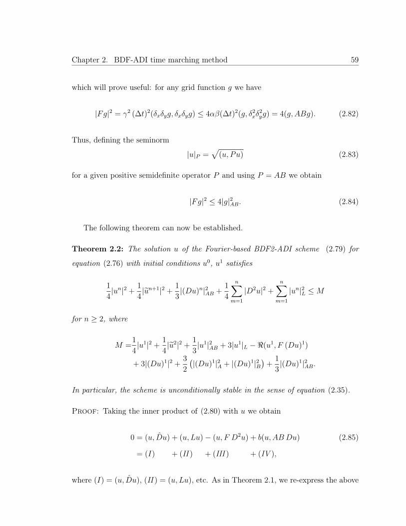
Chapter 2. BDF-ADI time marching method 59
which will prove useful: for any grid function g we have
|Fg|2 = γ2 (∆t)2(δxδyg, δxδyg) ≤ 4αβ(∆t)2(g, δ2xδ
2yg) = 4(g, ABg). (2.82)
Thus, defining the seminorm
|u|P =√
(u, Pu) (2.83)
for a given positive semidefinite operator P and using P = AB we obtain
|Fg|2 ≤ 4|g|2AB. (2.84)
The following theorem can now be established.
Theorem 2.2: The solution u of the Fourier-based BDF2-ADI scheme (2.79) for
equation (2.76) with initial conditions u0, u1 satisfies
1
4|un|2 +
1
4|un+1|2 +
1
3|(Du)n|2AB +
1
4
n∑m=1
|D2u|2 +n∑
m=1
|un|2L ≤M
for n ≥ 2, where
M =1
4|u1|2 +
1
4|u2|2 +
1
3|u1|2AB + 3|u1|L −<(u1, F (Du)1)
+ 3|(Du)1|2 +3
2
(|(Du)1|2A + |(Du)1|2B
)+
1
3|(Du)1|2AB.
In particular, the scheme is unconditionally stable in the sense of equation (2.35).
Proof: Taking the inner product of (2.80) with u we obtain
0 = (u, Du) + (u, Lu)− (u, F D2u) + b(u,ABDu) (2.85)
= (I) + (II ) + (III ) + (IV ),
where (I) = (u, Du), (II ) = (u, Lu), etc. As in Theorem 2.1, we re-express the above

Chapter 2. BDF-ADI time marching method 60
equation using telescoping and non-negative terms to obtain the desired energy bound.
The term (I) already occurs in the proof of Theorem 2.1; there we obtained the
relation
<(I ) =1
4D(|u|2 + |w|2) +
1
4|D2u|2, (2.86)
where w is defined in (2.58). The term (II ) = |u|2L, in turn, is non-negative by equa-
tion (2.81) and needs no further treatment. The remaining two terms are considered
in what follows.
(III ): This term presents the most difficulty, since F is not positive semi-definite. In
what follows the term (III ) is re-expressed as a a sum of two quantities, the first one
of which can be combined with a corresponding term arising from the quantity (IV )
to produce a telescoping term, and the second of which will be addressed towards the
end of the proof by utilizing Lemma 2.2.
Let v denote the time series obtained by shifting u backwards by one time step:
v = vn = un−1 : n ≥ 1; (2.87)
clearly we have
Du = u− v and D2u = Du−Dv. (2.88)
Thus, using the finite difference product rule (2.51) and the second relation in (2.88)
we obtain
(III ) = −(u, F D(Du)) = −(u,D F (Du))
= −D(u, F Du) + (Du, F Du)− (Du, F D2u)
= −D(u, F Du) + (Du, F Dv).
Applying the Cauchy-Schwarz inequality and Young’s inequality (2.70) with r = 6

Chapter 2. BDF-ADI time marching method 61
together with (2.84) we obtain
<(III ) ≥ −D<(u, F Du)− |Du| |F Dv|
≥ −D<(u, F Du)− 3|Du|2 − 1
12|F Dv|2
≥ −D<(u, F Du)− 3|Du|2 − 1
3|Dv|2AB. (2.89)
The last term in the above inequality will be used to form the desired telescoping
term with an associated expression in (IV ) below.
(IV ): Using the finite difference product rule (2.52) together with the fact that AB
is a Hermitian positive semi-definite operator we obtain
<(IV ) =2
3<(u,ABDu) =
2
3<(Du,ABu)
=1
3D(u,AB u) +
1
3(Du,ABDu)
=1
3D|u|2AB +
1
3|Du|2AB (2.90)
(see equation (2.83)). Substituting equations (2.86), (2.89) and (2.90) into equa-
tion (2.85) and taking real parts, we obtain
0 ≥1
4D(|u|2 + |w|2) +
1
4|D2u|2 + |u|2L −D<(u, F Du)− 3|Du|2
+1
3(|Du|2AB − |Dv|2AB) +
1
3D|u|2AB
=D
(1
4|u|2 +
1
4|w|2 +
1
3|u|2AB +
1
3|Du|2AB −<(u, F Du)
)+ |u|2L +
1
4|D2u|2 − 3|Du|2. (2.91)
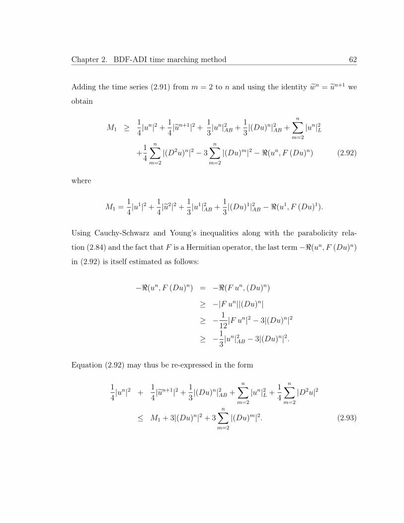
Chapter 2. BDF-ADI time marching method 62
Adding the time series (2.91) from m = 2 to n and using the identity wn = un+1 we
obtain
M1 ≥1
4|un|2 +
1
4|un+1|2 +
1
3|un|2AB +
1
3|(Du)n|2AB +
n∑m=2
|un|2L
+1
4
n∑m=2
|(D2u)n|2 − 3n∑
m=2
|(Du)m|2 −<(un, F (Du)n) (2.92)
where
M1 =1
4|u1|2 +
1
4|u2|2 +
1
3|u1|2AB +
1
3|(Du)1|2AB −<(u1, F (Du)1).
Using Cauchy-Schwarz and Young’s inequalities along with the parabolicity rela-
tion (2.84) and the fact that F is a Hermitian operator, the last term −<(un, F (Du)n)
in (2.92) is itself estimated as follows:
−<(un, F (Du)n) = −<(F un, (Du)n)
≥ −|F un||(Du)n|
≥ − 1
12|F un|2 − 3|(Du)n|2
≥ −1
3|un|2AB − 3|(Du)n|2.
Equation (2.92) may thus be re-expressed in the form
1
4|un|2 +
1
4|un+1|2 +
1
3|(Du)n|2AB +
n∑m=2
|un|2L +1
4
n∑m=2
|D2u|2
≤ M1 + 3|(Du)n|2 + 3n∑
m=2
|(Du)m|2. (2.93)

Chapter 2. BDF-ADI time marching method 63
Finally, applying Lemma 2.2 below to the last two terms on the right-hand side of
equation (2.93) we obtain
3|(Du)n|2 + 3n∑
m=2
|(Du)m|2 ≤ 3M2,
where the constant M2 is given by equation (2.95). Using this inequality to bound
the last two terms in equation (2.93) completes the proof of the theorem.
The following lemma, which provides a bound on sums of squares of the temporal
difference Du, is used in the proof of Theorem 2.2 above.
Lemma 2.2: The solution u of the Fourier-based BDF2-ADI scheme (2.79) for equa-
tion (2.76) with initial conditions u0, u1 satisfies
|(Du)n|2 + |un|2L +1
2
(|(Du)n|2A + |(Du)n|2B
)+
n∑m=2
|(Du)m|2 ≤M2 (2.94)
for n ≥ 2, where
M2 = |(Du)1|2 + |u1|2L +1
2
(|(Du)1|2A + |(Du)1|2B
). (2.95)
Proof: We start by taking the inner product of equation (2.80) with Du to obtain
0 = (Du, Du) + (Du,Lu)− (Du, F D2u) + b(Du,ABDu) (2.96)
= (I) + (II ) + (III ) + (IV ).
We now estimate each of the terms (I) through (IV ) in turn; as it will become
apparent, the main challenge in this proof is to estimate the term (III ).
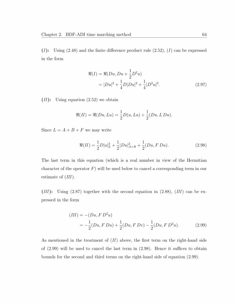
Chapter 2. BDF-ADI time marching method 64
(I): Using (2.48) and the finite difference product rule (2.52), (I) can be expressed
in the form
<(I) = <(Du,Du+1
2D2u)
= |Du|2 +1
4D|Du|2 +
1
4|D2u|2. (2.97)
(II ): Using equation (2.52) we obtain
<(II ) = <(Du,Lu) =1
2D(u, Lu) +
1
2(Du,LDu).
Since L = A+B + F we may write
<(II ) =1
2D|u|2L +
1
2|Du|2A+B +
1
2(Du, F Du). (2.98)
The last term in this equation (which is a real number in view of the Hermitian
character of the operator F ) will be used below to cancel a corresponding term in our
estimate of (III ).
(III ): Using (2.87) together with the second equation in (2.88), (III ) can be ex-
pressed in the form
(III ) = −(Du, F D2u)
= −1
2(Du, F Du) +
1
2(Du, F Dv)− 1
2(Du, F D2u). (2.99)
As mentioned in the treatment of (II ) above, the first term on the right-hand side
of (2.99) will be used to cancel the last term in (2.98). Hence it suffices to obtain
bounds for the second and third terms on the right-hand side of equation (2.99).

Chapter 2. BDF-ADI time marching method 65
To estimate the second term in (2.99) we consider the relation
1
2(Du, F Dv) =
1
2γ∆t (Du, δxδyDv) = −γ
4∆t (δxDu, δyDv)− γ
4∆t (δyDu, δxDv),
(2.100)
which follows from the fact that δx and δy are skew-Hermitian operators. Taking
real parts and applying the Cauchy-Schwarz and Young inequalities together with
the parabolicity condition (2.77) we obtain
1
2<(Du, F Dv) ≥−
√αβ
2∆t
(1
2
√α
β|δxDu|2 +
1
2
√β
α|δyDv|2
)
−√αβ
2∆t
(1
2
√β
α|δyDu|2 +
1
2
√α
β|δxDv|2
)=− 1
4∆t (α |δxDu|2 + β |δyDu|2)− 1
4∆t (α |δxDv|2 + β |δyDv|2)
=− 1
4|Du|2A+B −
1
4|Dv|2A+B. (2.101)
To estimate third term in (2.99) we once again use the Cauchy-Schwarz and Young
inequalities and we exploit the relation (2.84); we thus obtain
−1
2<(Du, F D2u) = −1
2<(F Du,D2u)
≥ −1
6|F Du|2 − 3
8|D2u|2
≥ −2
3|Du|2AB −
3
8|D2u|2. (2.102)
Taking the real part of (2.99) and using equations (2.101) and (2.102) we obtain
the relation
<(III ) ≥ −1
2<(Du, F Du)− 1
4|Du|2A+B −
1
4|Dv|2A+B −
2
3|Du|2AB −
3
8|D2u|2, (2.103)
which, as shown below, can be combined with the estimates for (I), (II ), and (IV )
to produce an overall estimate that consists solely of non-negative and telescoping

Chapter 2. BDF-ADI time marching method 66
terms—as desired.
(IV ): In view of (2.83) we see that (IV ) coincides with the P -seminorm of Du with
P = AB,
<(IV ) = (IV ) =2
3|Du|2AB, (2.104)
which, of course, is non-negative, and therefore this term does not require any further
treatment.
To complete the proof of the lemma we take real parts in equation (2.96) and we
substitute (2.97), (2.98), (2.103) and (2.104); the result is
0 ≥|Du|2 +1
4D|Du|2 − 1
8|D2u|2 +
1
2D|u|2L +
1
4|Du|2A+B −
1
4|Dv|2A+B
=|Du|2 − 1
8|D2u|2 +D
(1
4|Du|2 +
1
2|u|2L +
1
4|Du|2A+B
). (2.105)
The first two terms on the right-hand-side can be bounded by expanding |D2u|2 and
using Cauchy-Schwarz and Young’s inequalities to obtain
|Du|2 − 1
8|D2u|2 = |Du|2 − 1
8|Du−Dv|2 (2.106)
= |Du|2 − 1
8(|Du|2 + |Dv|2) +
1
4<(Du,Dv) (2.107)
≥ |Du|2 − 1
8(|Du|2 + |Dv|2)− 1
4|Du||Dv| (2.108)
≥ |Du|2 − 1
4(|Du|2 + |Dv|2) (2.109)
=1
2|Du|2 +
1
4D|Du|2. (2.110)
Substituting this result into (2.105), we obtain
0 ≥1
2|Du|2 +D
(1
2|Du|2 +
1
2|u|2L +
1
4|Du|2A+B
), (2.111)
which, as needed, is expressed as a sum of non-negative and telescoping terms. Adding

Chapter 2. BDF-ADI time marching method 67
the time-series (2.111) from m = 2 to n yields the desired equation (2.94), and the
proof is thus complete.
Remark 2.5: It is interesting to point out that Lemma 2.2 by itself implies a weak
stability result that follows from equation (2.94) and the Cauchy-Schwarz inequality:
|un| = |u1 +n∑
m=2
(Du)m|
≤ |u1|+n∑
m=2
|(Du)m|
≤ |u1|+(n
n∑m=2
|(Du)m|2) 1
2
≤ |u1|+√nM2, (2.112)
Theorem 2.2 provides a much tighter energy estimate than (2.112), of course.
2.3.4.1 Stability in non-periodic domain with Legendre collocation
The stability result for the parabolic equation can easily be extended to a non-periodic
setting using a Legendre polynomial collocation spatial approximation. Here we pro-
vide the main necessary elements to produce the extensions of the proofs. Background
on polynomial collocation methods may be found, e.g., in [57].
Under Legendre collocation we discretize the domain Ω = [−1, 1]×[−1, 1] by means
of the N + 1 Legendre Gauss-Lobatto quadrature nodes xj = yj (j = 0, . . . , N) in
each one of the coordinate directions, which defines the grid (xj, yk) : 0 ≤ j, k ≤ N(with x0 = y0 = −1 and xN = yN = 1). For real-valued grid functions f = (fjk) and
g = (gjk) we use the inner product
(f, g) =N∑j=0
N∑k=0
wjwkfjkgjk, (2.113)
where w` (0 ≤ ` ≤ N) are the Legendre Gauss-Lobatto quadrature weights. The

Chapter 2. BDF-ADI time marching method 68
interpolant fN of a grid function f is a linear combination of the form
fN(x, y) =N∑j=0
N∑k=0
fjkPj(x)Pk(y)
of Legendre polynomials Pj.
A certain exactness relation similar to the one we used in the Fourier case exists
in the Legendre context as well. Namely, for grid functions f and g for which the
product of the interpolants has polynomial degree ≤ 2N−1 in the x (resp. y) variable,
the j (resp. k) summation in the inner product (2.113) of the two grid functions is
equal to the integral of their corresponding polynomial interpolants with respect to
x (resp. y) [47, Sec. 5.2.1]—i.e.,
(f, g) =N∑k=0
∫ 1
−1
fN(x, yk)gN(x, yk) dx, (2.114a)
provided
deg(fN(x, yk)gN(x, yk)
)≤ 2N − 1 for all 0 ≤ k ≤ N,
and
(f, g) =N∑j=0
∫ 1
−1
fN(xj, y)gN(xj, y) dy, (2.114b)
provided
deg(fN(xj, y)gN(xj, y)
)≤ 2N − 1 for all 0 ≤ j ≤ N.
Thus, for example, defining the Legendre x-derivative operator δx as the derivative of
the Legendre interpolant (cf. (2.42)) (with similar definitions for δy, δxx, δyy etc.), the
exactness relation (2.114a) holds whenever one or both of the grid functions f and g
is a Legendre x-derivative of a certain grid function.
A stability proof for the parabolic equation with zero Dirichlet boundary condi-

Chapter 2. BDF-ADI time marching method 69
tions
Ut = αUxx + β Uyy + γ Uxy in Ω, U = 0 on ∂Ω,
can now be obtained by reviewing and modifying slightly the strategy presented for
the periodic case in Section 2.3.4. Indeed, the latter proof relies on the following
properties of the spatial differentiation operators:
1. The discrete first and second derivative operators are skew-Hermitian and Her-
mitian, respectively.
2. The operators A, B, L and AB defined in Section 2.3.4 are positive semi-definite.
Both of these results were established using the exactness relation between the dis-
crete and integral inner products together with vanishing boundary terms arising
from integration by parts—which also hold in the present case since the exactness
relations (2.114) are only ever required to convert inner products involving deriva-
tives, so that the degree of polynomial interpolants will satisfy the requirements of
the relations (2.114). Since all other aspects of the proofs in Section 2.3.4 are inde-
pendent of the particular spatial discretization or boundary conditions used, we have
the following theorem:
Theorem 2.3: The stability estimate given in Theorem 2.2 also holds on the domain
[−1, 1] × [−1, 1] with homogeneous boundary conditions using the Legendre Gauss-
Lobatto collocation method, where the inner products and norms are taken to be the
Legendre versions instead.
2.4 Quasi-unconditional stability for higher-order
BDF Fourier methods
This thesis does not present stability proofs for the BDF-ADI methods of order higher
than two. In order to provide some additional insights into the stability properties
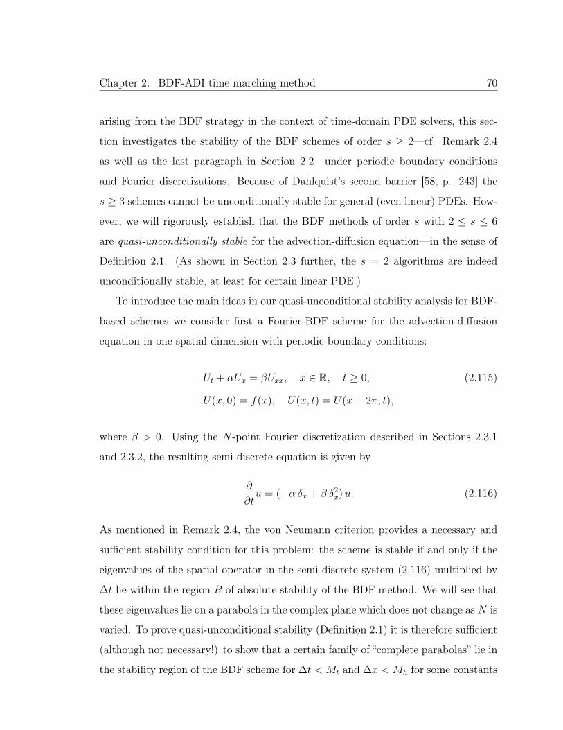
Chapter 2. BDF-ADI time marching method 70
arising from the BDF strategy in the context of time-domain PDE solvers, this sec-
tion investigates the stability of the BDF schemes of order s ≥ 2—cf. Remark 2.4
as well as the last paragraph in Section 2.2—under periodic boundary conditions
and Fourier discretizations. Because of Dahlquist’s second barrier [58, p. 243] the
s ≥ 3 schemes cannot be unconditionally stable for general (even linear) PDEs. How-
ever, we will rigorously establish that the BDF methods of order s with 2 ≤ s ≤ 6
are quasi-unconditionally stable for the advection-diffusion equation—in the sense of
Definition 2.1. (As shown in Section 2.3 further, the s = 2 algorithms are indeed
unconditionally stable, at least for certain linear PDE.)
To introduce the main ideas in our quasi-unconditional stability analysis for BDF-
based schemes we consider first a Fourier-BDF scheme for the advection-diffusion
equation in one spatial dimension with periodic boundary conditions:
Ut + αUx = βUxx, x ∈ R, t ≥ 0, (2.115)
U(x, 0) = f(x), U(x, t) = U(x+ 2π, t),
where β > 0. Using the N -point Fourier discretization described in Sections 2.3.1
and 2.3.2, the resulting semi-discrete equation is given by
∂
∂tu = (−α δx + β δ2
x)u. (2.116)
As mentioned in Remark 2.4, the von Neumann criterion provides a necessary and
sufficient stability condition for this problem: the scheme is stable if and only if the
eigenvalues of the spatial operator in the semi-discrete system (2.116) multiplied by
∆t lie within the region R of absolute stability of the BDF method. We will see that
these eigenvalues lie on a parabola in the complex plane which does not change as N is
varied. To prove quasi-unconditional stability (Definition 2.1) it is therefore sufficient
(although not necessary!) to show that a certain family of “complete parabolas” lie in
the stability region of the BDF scheme for ∆t < Mt and ∆x < Mh for some constants

Chapter 2. BDF-ADI time marching method 71
Mt and Mh. This follows from an application of Lemma 2.3, which establishes that
the stability regions of the BDF schemes contain such families of parabolas.
Lemma 2.3: Let Γm be a left-facing parabola passing through the origin in the com-
plex plane with focus −m/4 and vertical directrix passing through +m/4. Then, for
each 2 ≤ s ≤ 6, there exists a critical m-value, mC, such that the parabola Γm lies in
the stability region R of the BDF method of order s for all 0 ≤ m < mC.
Proof: The A-stability (Section 2.4) of the BDF method of order s = 2 implies
directly that all left-facing parabolas are contained in R, and thus mC = ∞ in this
case. The remaining cases (3 ≤ s ≤ 6) are considered next.
The parabola Γm coincides with the set Γm = w |w = − 1my2 − iy, y ∈ R . Let
Gm be the set of points to the left of the parabola together with the parabola itself.
Clearly, Gm equals the set of points w such that the distance d1 from w to the focus is
less than the distance d2 from w to the directrix. Equivalently, it is the set of points
such that d21 − d2
2 ≤ 0, where
d21 = |w +m/4|2
= (<w +m/4)2 + (=w)2
and
d22 = (<w −m/4)2.
It follows that
Gm = w | (=w)2 +m<w < 0 .
Let
m(x) = sup
(=w)2
−<w |w ∈ R, <w = x
. (2.117)
The above definition of m(x) is such that the parabola Γm intersects the boundary

Chapter 2. BDF-ADI time marching method 72
of the stability region R at a point z0 with real part x, and the vertical segment
z|<z = x, =z < =z0 is contained in R. Since Gm1 ⊂ Gm2 if and only if m1 ≤ m2,
it follows that the the stability region R contains Gm provided m ≤ m(x) for all
negative numbers x. Clearly, the quantity
mC = inf m(x) |x < 0 (2.118)
is the “critical” m value—that is, mC is the largest such value of m. It follows that
Gm ⊂ R if and only if m ≤ mC . We now show that mC > 0 for all BDF methods of
orders 3 ≤ s ≤ 6.
The BDF methods under consideration are A(0)-stable [58, Ch. 3.12]—that is,
using a polar coordinate system with angles measured in the counter-clockwise di-
rection from the positive real axis, there is an angle α0 > 0 such that the wedge
r ei(π+θ) | r ≥ 0, |θ| ≤ α0 is part of the stability region. Clearly, w ∈ R provided
=w < <w tanα0. Therefore, m(x) ≥ −x tan2 α0 > 0 for any x < 0 and all that is left
is to ensure that m(x) is positive in a neighborhood of x = 0.
In terms of the stability polynomial [61, p. 153] p(ζ, z) associated with a given
multistep method, R is the set of z such that the roots of p (as a function of ζ) lie in
the closed unit disk, with only simple roots on the boundary. For the order-s BDF
method, the stability polynomial is given by
p(ζ, z) = (1− bz)ζs −s−1∑j=0
ajζs−1−j.
Using the boundary locus method [58, Ch. 3.8] we let the boundary of the stability
region be given by the implicit relation p(eiθ, z) = 0 for θ ∈ [0, 2π] (where θ denotes
the polar angle in the complex z plane). Solving for z we have
z(θ) =1
b
(1−
s−1∑j=0
aje−i(j+1)θ
),
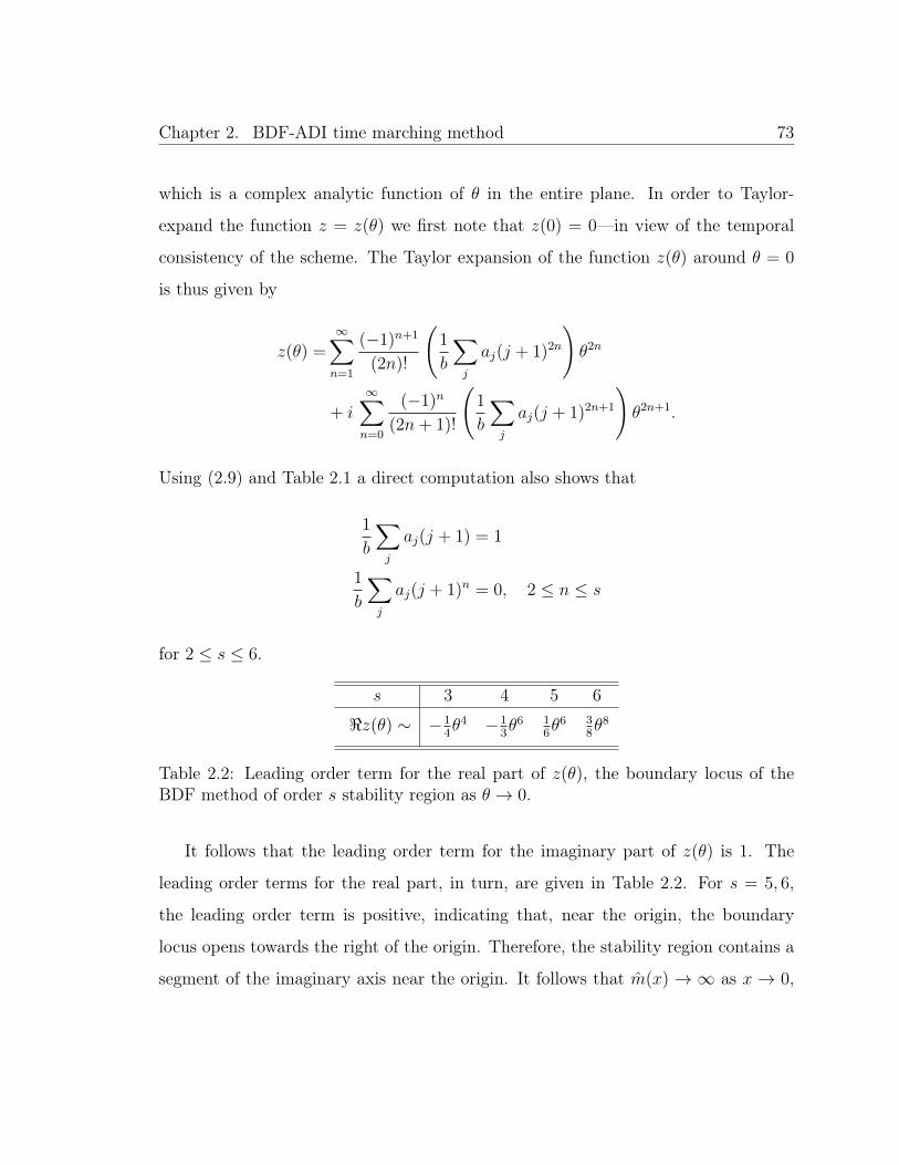
Chapter 2. BDF-ADI time marching method 73
which is a complex analytic function of θ in the entire plane. In order to Taylor-
expand the function z = z(θ) we first note that z(0) = 0—in view of the temporal
consistency of the scheme. The Taylor expansion of the function z(θ) around θ = 0
is thus given by
z(θ) =∞∑n=1
(−1)n+1
(2n)!
(1
b
∑j
aj(j + 1)2n
)θ2n
+ i
∞∑n=0
(−1)n
(2n+ 1)!
(1
b
∑j
aj(j + 1)2n+1
)θ2n+1.
Using (2.9) and Table 2.1 a direct computation also shows that
1
b
∑j
aj(j + 1) = 1
1
b
∑j
aj(j + 1)n = 0, 2 ≤ n ≤ s
for 2 ≤ s ≤ 6.
s 3 4 5 6
<z(θ) ∼ −14θ4 −1
3θ6 1
6θ6 3
8θ8
Table 2.2: Leading order term for the real part of z(θ), the boundary locus of theBDF method of order s stability region as θ → 0.
It follows that the leading order term for the imaginary part of z(θ) is 1. The
leading order terms for the real part, in turn, are given in Table 2.2. For s = 5, 6,
the leading order term is positive, indicating that, near the origin, the boundary
locus opens towards the right of the origin. Therefore, the stability region contains a
segment of the imaginary axis near the origin. It follows that m(x) → ∞ as x → 0,

Chapter 2. BDF-ADI time marching method 74
and, thus, mC is positive. For s = 3, 4, it also follows that
m(0) = limθ→0
(=z(θ))2
−<z(θ)
=∞.
Therefore the critical constant mC is positive for BDF schemes of order 3 ≤ s ≤ 6
and the proof is complete.
Remark 2.6: Equations (2.117) and (2.118) can be used to evaluate numerically the
constant mC for any given s; the results for each BDF method of orders 3 through 6
are summarized in Table 2.3.
s 3 4 5 6mC 14.0 5.12 1.93 0.191
Table 2.3: Numerical estimate of the constant mC such that for all m < mC theparabola Γm described in Lemma 2.3 is contained in the region of absolute stabilityof the BDF method of order s. By Theorem 2.4, the order-s BDF method applied tothe advection-diffusion equation ut + αux = β uxx with Fourier collocation is stablefor all ∆t < β
α2mC
.
Theorem 2.4: Let 2 ≤ s ≤ 6. The solution of the problem (2.115) by the s-th order
Fourier-based BDF scheme described in this section is quasi-unconditionally stable,
with Mh = ∞ and Mt = βα2mC (Mt = ∞ for α = 0), where mC is a real constant
which depends only on s.
Proof: Applying the discrete Fourier transform,
uk =1
N + 1
N∑j=0
uje−ixjk, −N
2≤ k ≤ N
2,

Chapter 2. BDF-ADI time marching method 75
to equation (2.116), we have the set of ODEs
∂
∂tuk = −(iαk + βk2) uk (2.119)
for the Fourier coefficients uk. It is clear from this transformed equation that the
eigenvalues of the spatial operator for the semi-discrete system are given by
λ(k) = −(iαk + βk2). (2.120)
Using von Neumann stability analysis, it is sufficient to show that these eigenvalues
multiplied by ∆t lie in the stability region of the BDF method.
Let z = λ∆t where λ = λ(k) is an eigenvalue of the semi-discrete system (2.116).
If α = 0, then z is a non-positive real number. In view of the A(0)-stability of the
BDF methods, we immediately see that the methods are unconditionally stable in
this case.
Let us now consider the case α 6= 0. We must find the values of ∆t for which the
complex numbers
zk = −β∆t k2 − iα∆t k
= − β
α2∆t(α∆t k)2 − i(α∆t k)
= − 1α2∆tβ
(α∆t k)2 − i(α∆t k) with − N
2≤ k ≤ N
2(2.121)
lie in the stability region R. But from (2.121) it is clear that z lies on the set
Γm = w |w = − 1my2−iy, y ∈ R withm = α2∆t
β, which is a left-facing parabola with
focus −m/4 and vertical directrix passing through the point +m/4. By Lemma 2.3,
it follows that the parabola lies in the stability region R for all m satisfying
m < mC =⇒ ∆t <β
α2mC .

Chapter 2. BDF-ADI time marching method 76
Furthermore, the above condition holds for all spatial discretizations, so thatMh =∞and the proof is complete.
We now establish the quasi-unconditional stability of the BDF methods applied
to the two- and three-dimensional advection diffusion equation
ut + α · ∇u = β∆u, in [0, 2π]d, d = 2, 3 (2.122)
with periodic boundary conditions, where α = (α1, α2)T and α = (α1, α2, α3)T for d =
2 and 3 respectively. To define a single mesh-size parameter h and quasi-unconditional
stability constant Mh, we fix positive integers r1 and r2 and discretize the domain
with Nx + 1 points in the x direction, Ny + 1 = r1Nx + 1 points in the y direction,
and Nz + 1 = r2Nx + 1 points in the z direction (Nx even). The mesh size parameter
is then h = 2π/(Nx + 1).
Theorem 2.5: The solution of (2.122) using the BDF scheme of order s (not ADI!)
with 3 ≤ s ≤ 6 and the Fourier collocation discretization is quasi-unconditionally
stable with constants Mt = |α|2βmC and Mh =∞.
Proof: We present the proof for the d = 2 case; the same procedure yields the d = 3
result.
Substituting the Fourier series
u(x, y) =
Nx2∑
k=−Nx2
Ny2∑
`=−Ny2
uk`ei(kx+`y)
into equation (2.122), we have the system of ODEs for the Fourier coefficients uk`
∂uk`∂t
=(−i(α1k + α2`)− β(k2 + `2)
)uk`.
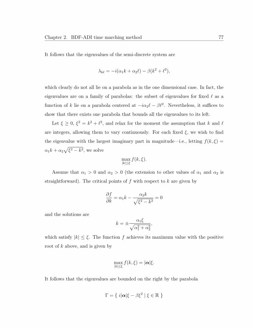
Chapter 2. BDF-ADI time marching method 77
It follows that the eigenvalues of the semi-discrete system are
λk` = −i(α1k + α2`)− β(k2 + `2),
which clearly do not all lie on a parabola as in the one dimensional case. In fact, the
eigenvalues are on a family of parabolas: the subset of eigenvalues for fixed ` as a
function of k lie on a parabola centered at −iα2` − β`2. Nevertheless, it suffices to
show that there exists one parabola that bounds all the eigenvalues to its left.
Let ξ ≥ 0, ξ2 = k2 + `2, and relax for the moment the assumption that k and `
are integers, allowing them to vary continuously. For each fixed ξ, we wish to find
the eigenvalue with the largest imaginary part in magnitude—i.e., letting f(k, ξ) =
α1k + α2
√ξ2 − k2, we solve
max|k|≤ξ
f(k, ξ).
Assume that α1 > 0 and α2 > 0 (the extension to other values of α1 and α2 is
straightforward). The critical points of f with respect to k are given by
∂f
∂k= α1k −
α2k√ξ2 − k2
= 0
and the solutions are
k = ± α1ξ√α2
1 + α22
,
which satisfy |k| ≤ ξ. The function f achieves its maximum value with the positive
root of k above, and is given by
max|k|≤ξ
f(k, ξ) = |α|ξ.
It follows that the eigenvalues are bounded on the right by the parabola
Γ = i|α|ξ − βξ2 | ξ ∈ R

Chapter 2. BDF-ADI time marching method 78
regardless of the values of Nx and Ny. The theorem now follows from an application
of Lemma 2.3.
2.4.1 Order-s BDF methods outside the region of quasi-
unconditional stability
(a) (b) (c)
Figure 2.3: Demonstration of a CFL-like stability constraint when ∆t is outside therectangular window of quasi-unconditional stability for the advection-diffusion equa-tion with α = 1.0 and β = 0.05 (parameters selected for clarity of visualization.Theoretical value: Mt = 0.0965 for this selection of physical parameters). The eigen-values multiplied by ∆t (black dots) are plotted together with the boundary of theBDF5 stability region (dashed grey curve; cf. Figure 2.1). (a) Using N + 1 = 9 gridpoints and time step ∆t = 0.23 all eigenvalues lie within the stability region. (b) Thenumber of points is increased to N +1 = 19 while the time step is held constant. Theten additional eigenvalues are not in the stability region, which indicates the methodis unstable for these parameter values. (c) The number of points is again N + 1 = 19,but the time step is reduced to ∆t = 0.12, causing all eigenvalues to be contained inthe stability region.
Theorems 2.4 and 2.5 should not be viewed as a suggestion that the s-th order
BDF methods are not stable when the constraints in the theorem are not satisfied.

Chapter 2. BDF-ADI time marching method 79
(a) (b) (c)
Figure 2.4: Continuation of Figure 2.3. (a) The time step is ∆t = 0.12 (as inFigure 2.3(c)) and the number of grid points is increased to N + 1 = 35. Once again,some eigenvalues do not lie in the stability region. (b) The number of grid points isheld at N + 1 = 35 while the time step is reduced to ∆t = Mt = 0.0965, which isthe maximum allowed for the window of quasi-unconditional stability. All eigenvaluesnow lie in the stability region. (c) With ∆t = 0.0965, additional eigenvalues (arisingfrom further increasing the number of grid points) remain within the stability region,thus demonstrating the quasi-unconditional stability of the BDF scheme of order 5.
Indeed, while, by definition, for ∆t > Mt the complete parabolic region Γm passes
through the region where the BDF method is unstable (as demonstrated in Figure 2.3
as well as in the first two images in Figure 2.4), stability can still be ensured for such
a value of ∆t provided adequate values of the discretization parameter N + 1 = 2π/h
are used. Indeed, taking into account that only a bounded segment in the parabola is
actually relevant to the stability of the ODE system that results for each fixed value
of N , we see that stability may be ensured provided this particular segment, and not
necessarily the complete parabola Γm, is contained in the stability region of the s-th
order BDF algorithm.
From equation (2.121) we see that increasing values of N lead to corresponding
increases in the length of the parabolic segment on which the eigenvalues actually lie,

Chapter 2. BDF-ADI time marching method 80
while decreasing ∆t results in reductions of both the length of the relevant parabolic
segment as well as the width of the parabola itself. Therefore, for ∆t > Mt, increasing
the number of grid points will inevitably cause some eigenvalues to eventually enter
the region of instability. But stability can be restored by a corresponding reduction
in ∆t—see Figure 2.3. This argument suggests that a CFL condition of the form
∆t ≤ C/N exists for ∆t > Mt. Of course, when ∆t is reduced to the value Mt or
below, then no increases in N (reductions in h) result in instability—as demonstrated
in Figure 2.4. We may thus emphasize: within the quasi-unconditional stability
window no such CFL-like stability constraints exist.
Figure 2.5: Maximum stable ∆t versus spatial mesh size h for Fourier-based BDFand AB methods of orders three and four when applied to the advection-diffusionequation (2.115), with α = 1, β = 10−2 on the left and α = 1, β = 10−2 on the right.
To better understand when the BDF methods are preferable to an explicit scheme,
we compare their stability to that of the explicit Adams-Bashforth (AB) multistep
methods. For a given number of discretization points N + 1 and physical parameter
values α and β, we can use the equation for the eigenvalues (2.120) of the advection-
diffusion equation and the boundary locus z(θ) of the stability regions to estimate
the maximum stable ∆t by solving z(θ) = λ(N/2) ∆t for θ and ∆t.
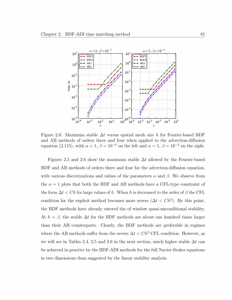
Chapter 2. BDF-ADI time marching method 81
Figure 2.6: Maximum stable ∆t versus spatial mesh size h for Fourier-based BDFand AB methods of orders three and four when applied to the advection-diffusionequation (2.115), with α = 1, β = 10−3 on the left and α = 1, β = 10−4 on the right.
Figures 2.5 and 2.6 show the maximum stable ∆t allowed by the Fourier-based
BDF and AB methods of orders three and four for the advection-diffusion equation,
with various discretizations and values of the parameters α and β. We observe from
the α = 1 plots that both the BDF and AB methods have a CFL-type constraint of
the form ∆t < Ch for large values of h. When h is decreased to the order of β the CFL
condition for the explicit method becomes more severe (∆t < Ch2). By this point,
the BDF methods have already entered the of window quasi-unconditional stability.
At h = β, the stable ∆t for the BDF methods are about one hundred times larger
than their AB counterparts. Clearly, the BDF methods are preferable in regimes
where the AB methods suffer from the severe ∆t < Ch2 CFL condition. However, as
we will see in Tables 2.4, 2.5 and 2.6 in the next section, much higher stable ∆t can
be achieved in practice by the BDF-ADI methods for the full Navier-Stokes equations
in two dimensions than suggested by the linear stability analysis.

Chapter 2. BDF-ADI time marching method 82
2.4.2 Quasi-unconditional stability: linearized and full
Navier-Stokes equations
To further extend the analysis provided in the previous sections for the advection-
diffusion equation, here we consider the Navier-Stokes equations linearized about a
temperature and density equal to 1 and a non-dimensional constant velocity U in the
x direction, so that T = 1 + T , ρ = 1 + ρ, u = U + u, v = 0, and w = 0, where
the perturbations are denoted with a tilde. Inserting these expressions into (1.4) and
neglecting terms that are quadratic in the perturbations, the linearized equations
ρt + U ρx + ux = 0 (2.123a)
ut + U ux +1
γMa2(Tx + ρx) =
4
3
1
Reuxx (2.123b)
Tt + U Tx + (γ − 1)ux =γ
Re PrTxx (2.123c)
result; in what follows the tildes are dropped for simplicity. The above equations can
thus be re-expressed in the matrix form
Qt = LQ,
where Q = (ρ, u, T )T,
L = −(M1
∂
∂X+
1
ReM2
∂2
∂X2
),
and the matrices M1 and M2 are given by
M1 =
U 1 0
1γMa2
U 1γMa2
0 (γ − 1) U
and M2 = diag
(0,
4
3,γ
Pr
).
Chapter 2. BDF-ADI time marching method 83
Take the domain to be x ∈ [0, 2π] with periodic boundary conditions and consider
solutions of the form Q = (ρ, u, T )T, with ρ = u = T = exp( ikx ) for some integer k.
These solutions satisfy
Qt =(−iM1 k − δM2 k
2)Q., (2.124)
where δ = Re−1.
To carry the analysis further, we use perturbation theory in the limit of small δ
(large Reynolds number), which is consistent with the continuum fluid approximation
and with non-negligible compressibility effects. The continuum limit is characterized
by small Knudsen number (Kn 1), which is the ratio of the mean free path of
the molecules in the gas to the macroscopic length scale of the problem. By the
von Karman relation [78, p. 60], the Knudsen number is proportional to Ma/Re.
Accordingly, for the present analysis we assume Ma Re−1 1 and we linearize the
equations accordingly. Further, compressibility effects become negligible as Ma→ 0.
Therefore, we also take the Mach number to be of order one or greater, which together
with the von Karman relation implies δ = Re−1 1.
The eigenvalues of the matrix in parenthesis on the right-hand side of equa-
tion (2.124) can now be approximated by means of a perturbation series in δ. Let
λ =∑∞
j=0 δjλj be such an eigenvalue, i.e., it is a root of the characteristic equation
det(λI − iM1 k + δM2 k
2)
= 0. (2.125)
Dropping terms of order δ and higher, we recover the eigenvalues of the linearized
Euler equations:
λ0 ∈iUk, i
(U +
1
Ma
)k, i
(U − 1
Ma
)k
.
Expanding equation(2.125), keeping terms up to first order in δ and solving for λ1 we

Chapter 2. BDF-ADI time marching method 84
have
λ1 =λ0Ma2
(γ + 4
3Pr)
(2iUk − λ0) k2 + Ma2U2((γ + 4
3Pr)− 1)k4
Pr (3Ma2U2 − 1) k2 + λ0Ma2Pr (2iUk − λ0).
The λ1 are determined by substituting the three different values of λ0. The eigenvalues
of L corresponding to the eigenvector Q can then be approximated as
λ1(k) = iUk + δ1
Prk2 +O(δ2), (2.126a)
λ2(k) = i
(U +
1
Ma
)k + δ
(2
3+γ − 1
2 Pr
)k2 +O(δ2), (2.126b)
λ3(k) = i
(U − 1
Ma
)k + δ
(2
3+γ − 1
2 Pr
)k2 +O(δ2). (2.126c)
For each λ, the first term is the leading order term of the imaginary part of the
eigenvalue, and the second term is the leading order term of the real part. Compar-
ing (2.126) to (2.120), we see that the asymptotic behavior for large Reynolds number
is like that of the advection-diffusion equation. The first eigenvalue corresponds to
convective waves and the second two eigenvalues to acoustic waves. Extending the
analysis further, we can estimate the constant Mt of quasi-unconditional stability for
the linearized Navier-Stokes equations:
Mt ∼4Pr + 3(γ − 1)
6(|u|max + Ma−1)2Pr RemC . (2.127)
Tables 2.4, 2.5 and 2.6 show the numerically estimated maximum stable ∆t for the
full Navier-Stokes equations in two dimensional space, using the Chebyshev colloca-
tion method described in section 2.5 in the unit square (x, y) ∈ [0, 1]× [0, 1] at Mach
number 0.9 and various Reynolds numbers and discretizations. The initial condition
is u = 0, ρ = T = 1 and a source term of the form
f(x, y, t) = A sin(2πt) exp
(− 1
2σ2
((x− x0)2 + (y − y0)2
))
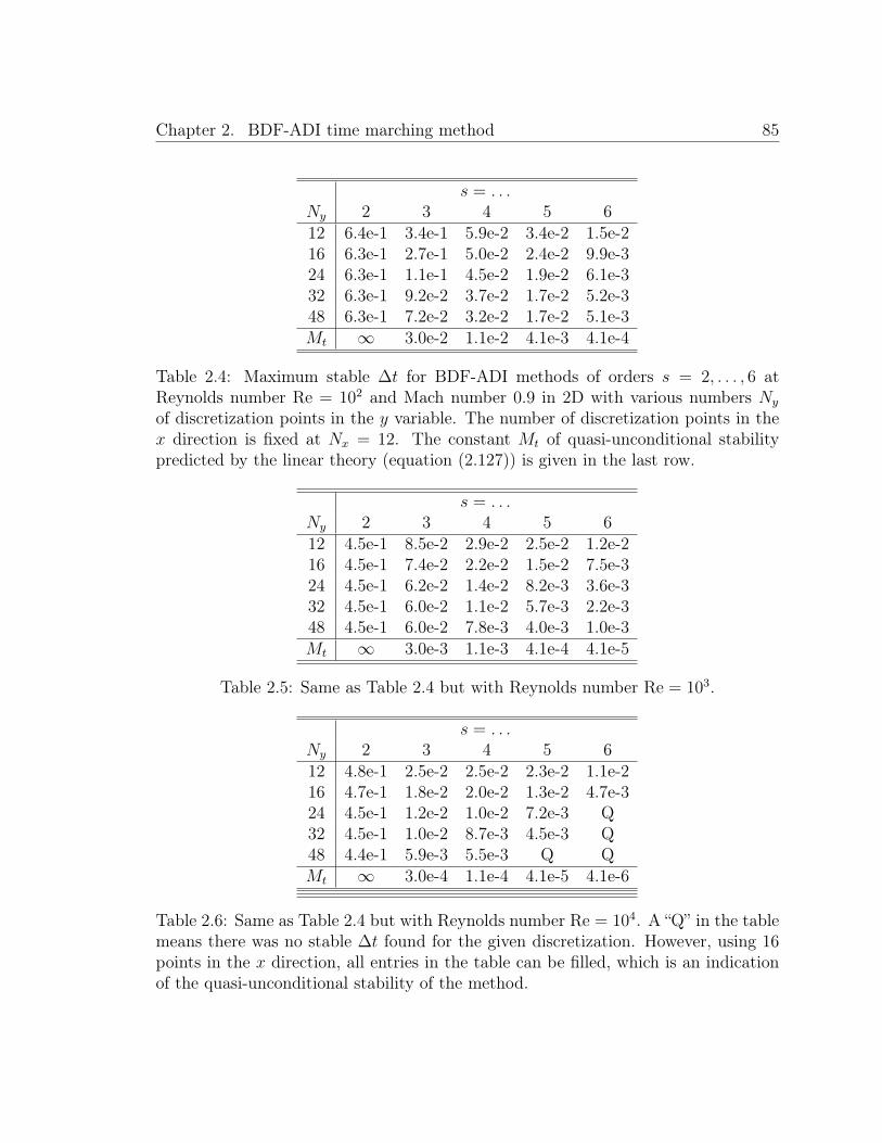
Chapter 2. BDF-ADI time marching method 85
s = . . .Ny 2 3 4 5 612 6.4e-1 3.4e-1 5.9e-2 3.4e-2 1.5e-216 6.3e-1 2.7e-1 5.0e-2 2.4e-2 9.9e-324 6.3e-1 1.1e-1 4.5e-2 1.9e-2 6.1e-332 6.3e-1 9.2e-2 3.7e-2 1.7e-2 5.2e-348 6.3e-1 7.2e-2 3.2e-2 1.7e-2 5.1e-3Mt ∞ 3.0e-2 1.1e-2 4.1e-3 4.1e-4
Table 2.4: Maximum stable ∆t for BDF-ADI methods of orders s = 2, . . . , 6 atReynolds number Re = 102 and Mach number 0.9 in 2D with various numbers Ny
of discretization points in the y variable. The number of discretization points in thex direction is fixed at Nx = 12. The constant Mt of quasi-unconditional stabilitypredicted by the linear theory (equation (2.127)) is given in the last row.
s = . . .Ny 2 3 4 5 612 4.5e-1 8.5e-2 2.9e-2 2.5e-2 1.2e-216 4.5e-1 7.4e-2 2.2e-2 1.5e-2 7.5e-324 4.5e-1 6.2e-2 1.4e-2 8.2e-3 3.6e-332 4.5e-1 6.0e-2 1.1e-2 5.7e-3 2.2e-348 4.5e-1 6.0e-2 7.8e-3 4.0e-3 1.0e-3Mt ∞ 3.0e-3 1.1e-3 4.1e-4 4.1e-5
Table 2.5: Same as Table 2.4 but with Reynolds number Re = 103.
s = . . .Ny 2 3 4 5 612 4.8e-1 2.5e-2 2.5e-2 2.3e-2 1.1e-216 4.7e-1 1.8e-2 2.0e-2 1.3e-2 4.7e-324 4.5e-1 1.2e-2 1.0e-2 7.2e-3 Q32 4.5e-1 1.0e-2 8.7e-3 4.5e-3 Q48 4.4e-1 5.9e-3 5.5e-3 Q QMt ∞ 3.0e-4 1.1e-4 4.1e-5 4.1e-6
Table 2.6: Same as Table 2.4 but with Reynolds number Re = 104. A “Q” in the tablemeans there was no stable ∆t found for the given discretization. However, using 16points in the x direction, all entries in the table can be filled, which is an indicationof the quasi-unconditional stability of the method.

Chapter 2. BDF-ADI time marching method 86
is added to the u equation, with parameters A = 6.0, σ2 = 0.05, x0 = y0 = 0.5. The
boundary conditions at y = 0, 1 are no-slip isothermal (u = 0, T = 1) and there is
a sponge layer (see equation (4.3)) of thickness 0.1 and amplitude 2.0 at x = 0, 1.
The method was determined to be stable for a given ∆t if the solution did not blow
up for 20000 time steps or for the number of time steps required to exceed t = 100,
whichever was greater.
Tables 2.4, 2.5 and 2.6 suggest that quasi-unconditional stability indeed exists
even for the full Navier-Stokes equations. Furthermore, we observe that the BDF-
ADI methods seem to enjoy stability for ∆t far greater than those predicted by the
linear stability analysis. In particular, the tables suggest that the BDF-ADI methods
may be particularly advantageous when a very fine mesh is only required in one of
the spatial dimensions.
2.5 Numerical implementation
In this section we present a spatial discretization for the semi-discrete BDF-ADI
schemes considered in this chapter and in Section 4.1. Spatial discretizations of vari-
ous kinds can be used in our context, including finite-difference, polynomial-spectral,
and Fourier-continuation discretizations (as in the following chapter). For the sake of
definiteness we restrict our treatment to the Chebyshev-collocation spatial approxi-
mation, which is the discretization we use for the numerical examples of the BDF-ADI
method in single domains (see Section 4.1). Details concerning Chebyshev collocation
can be found, e.g., in [10,57]; the text in the following section includes a brief overview
as well as a few specifics associated with our two-dimensional implementation. Ex-
tensions to the three-dimensional case do not present any additional difficulties. We
also note that many of the same elements described in the framework below apply to
FC and other spatial discretizations as well.

Chapter 2. BDF-ADI time marching method 87
2.5.1 Spectral collocation
The Fourier-spectral collocation method was described in Sections 2.3.1 and 2.3.2;
here we briefly outline the corresponding Chebyshev discretization that also is incor-
porated in our test solvers. For simplicity the description in this section is restricted
to two spatial dimensions and it assumes the domain is discretized by means of N +1
Gauss-Lobatto Chebyshev nodes in both the ξ and η directions:
ξi = − cos(πi/N) , i = 0, . . . , N
ηj = − cos(πj/N) , j = 0, . . . , N.
The actual solvers we use are not so restricted: they are applicable to two- and three-
dimensional problems, and they can use different numbers of discretization points in
the various coordinate directions.
By analogy with Section 2.3.1, grid functions Qij ∼ Q(ξi, ηj) for the solution Q are
used together with the associated Lagrange interpolating polynomials QN(ξ, η). The
discrete ξ and η spatial differentiation operators, in turn, are given by the Chebyshev
derivative operator which, as is well known, can be evaluated efficiently by means of
the fast cosine transform.
Using the Chebyshev (resp. Fourier-spectral) discretizations mentioned above,
the one-dimensional boundary value problems given by the ODEs (2.24) and the
boundary conditions (2.26) (resp. 2π-periodic boundary conditions) become systems
of linear equations. In order to fully take advantage of the fast cosine transform and
fast Fourier transform we solve these systems by means of the GMRES iterative solver
with second order finite difference preconditioner (cf. [10, p. ] and [17]).
For both Chebyshev and Fourier-spectral discretizations, an exponential filter [44],
which does not degrade the s-th order accuracy of the method (cf. [2, Sec. 4.3]), is
employed to eliminate high-frequency aliasing errors and thus ensure stability. In
the Chebyshev case, for example, the filtered coefficients cn for a given function
Chapter 2. BDF-ADI time marching method 88
f =∑
n cnTn(x) are given by
cn = exp
(−α( nN
)2p)cn.
For all of the results presented in Section 4.1 we have set α = 16 log 10 and p = 8.
The filter is applied at the end of the time step to each line of discretization points in
each dimension, requiring one fast cosine transform per line to obtain the coefficients
cn, and one transform to obtain the filtered physical function values.
The transformation of the equations to general coordinates requires the metric
terms ξx, ξy, etc; see Section 2.1.2. The solvers presented in this thesis use the so-
called “invariant form” of these metric terms [86], but other (accurate) alternatives
could be equally advantageous. The derivatives of the physical coordinates (xξ, xη,
etc.) needed in the actual expressions for the metric terms are produced by means of
the discrete derivative operators implicit in the Chebyshev or Fourier spatial approx-
imation used in each case.
2.5.2 Overall algorithmic description and treatment of bound-
ary values
Any successful algorithm for the Navier-Stokes equations must address the salient
difficulty posed by the lack of a physical boundary condition for the density ρ. This
section thus provides an overall description of the proposed BDF-ADI schemes, with
emphasis on topics concerning boundary conditions. Some comments are also pre-
sented with regards to the impact of boundary corners and edges on stability and
accuracy.
Given the elements described in previous parts of this chapter, the BDF-ADI al-
gorithms of s-th order of temporal accuracy can now be described in rather simple
terms—except perhaps for some details concerning boundary values of the fluid den-
sity, which require a few additional considerations. The absence of a density bound-

Chapter 2. BDF-ADI time marching method 89
ary condition has previously been successfully addressed by means of discretization
strategies based on use of staggered grids see, e.g., [18, Ch. 4.6] and the references
therein. In some such strategies the velocity and the temperature are collocated on
a Gauss-Lobatto grid while the density is collocated on a Gauss grid—so that the
density mesh contains no boundary points, and therefore no density boundary condi-
tions are needed. In the context of ADI-based methods such as the ones considered in
this chapter, however, it is not clear that a natural staggered-grid ADI method could
be designed—since the ADI approach requires solution of one-dimensional boundary
value problems which couple all field components. An alternative approach is pro-
posed in this thesis. This method uses the same Gauss-Lobatto grid for all unknowns,
including the density, and therefore it requires determination of the boundary values
of the density as part of the overall solution.
We describe our implementation for spatially two-dimensional problems; exten-
sion to three dimensions is analogous. The main observation is as follows: throughout
the domain (including the boundary) the density is entirely determined by the equa-
tions (2.24). In particular, the density boundary values at t = tn+1 can be obtained
by interpreting equation (2.24b) for each j line (0 ≤ j ≤ N) as a linear system satis-
fied by (d+ 2)(N − 1) + 2 unknowns, namely, the discrete values Qn+1jk of the vector
Q = (uT, T, ρ)T that correspond to discretization points in the interior of the PDE
domain (1 ≤ k ≤ N−1) together with the density boundary values (ρn+1jk for k = 0 and
N). Clearly, collocation of (2.24b) at all interior points along a relevant coordinate
segment furnishes (d + 2)(N − 1) equations for these unknowns. The necessary two
additional equations are obtained by enforcing the portion of (2.24b) that arises from
the mass conservation equation at each one of the two boundary points k = 0 and
k = N . Note that in order to formulate this system of (d+ 2)(N − 1) + 2 equations,
the values of Q = (uT, T, ρ)T at all interior discretization points and boundary points
must be available for all time steps t` with n− s+ 1 ≤ ` ≤ n, as well as the values of
u and T at the boundary points at time tn+1 (using the boundary conditions (2.26))

Chapter 2. BDF-ADI time marching method 90
and the values of Q∗ = ((u∗)T, T ∗, ρ∗)T at interior and boundary points, which are
provided by the previous half-step in the ADI process. Using such data the algorithm
produces the corresponding interior and boundary values of Qn+1jk .
In order to obtain the necessary values of Q∗ at all discretization points, we note
that equation (2.24a) provides, for each k line (0 ≤ k ≤ N), a similar linear system
of (d + 2)(N − 1) + 2 unknowns—the values of Q∗jk in the interior of the domain
(1 ≤ j ≤ N − 1) together with the intermediate density ρ∗ at the boundary points
(j = 0, N). These equations are obtained by collocating the equations (2.24a) at the
interior points, as well as the mass conservation component of (2.24a) at the boundary
points. The right-hand side of this linear system, in turn, requires the values of Q at
interior discretization points and boundary points for a few time steps t` with ` ≤ n,
as well as the values of u and T at the boundary points at time tn+1 (using (2.26a)), all
of which are either data given as part of the problem, or were otherwise produced by
the algorithm over a few previous time steps. Thus, the system for the intermediate
unknowns Q∗ is closed: the solution Qn+1 can be obtained for all n by means of the
procedure described in this paragraph and the previous one provided the solution is
known for the first s time steps.
Although the solvers enjoy quasi-unconditional stability for the implementation
described thus far, a reduction in the temporal order of accuracy may occur due to
the solutions un+1 and T n+1 of the ODEs in the second step of (2.24) for lines along
the boundaries not satisfying the physical boundary conditions prescribed there. Re-
imposing the boundary conditions for u and T along these boundaries eliminates this
problem without affecting stability.
We emphasize here that no special boundary conditions are required for either the
intermediate density ρ∗ or the final density ρn+1. The density is determined entirely
by the equations (2.24) throughout the domain, up to and including the boundary.
Furthermore, the presence of corners does not impact the stability of the solver: no
special boundary treatment for the corners of the domain are necessary.

Chapter 2. BDF-ADI time marching method 91
Remark 2.7: Although corners do not affect the stability of our solvers, we note here
that the spatial accuracy may deteriorate (as is well known for spectral discretiza-
tions [10, Ch. 6.12]) which leads to a corresponding loss of time accuracy order.
This problem is alleviated by using a multi-domain decomposition that smooths out
all corners, which is considered in Chapter 3. Nevertheless, the numerical examples
in Section 4.1 show the correct order of time accuracy of the solvers in a domain with
no corners (an annulus) and in Cartesian domains with a manufactured solution.
A wide variety of effective strategies are available for the evaluation of the solution
for the initial s time steps. The simplest one of them is the one by which the solution
is ramped-up from a constant field state (usually zero for all velocities and one for the
density and temperature). But in some situations genuine initial value problems must
be solved; see, e.g., the example provided in Section 4.1 involving flow in an annulus,
where the density has a non-constant initial condition. In such cases use of explicit
solvers is sometimes recommended, but such explicit solvers generally require use of
significantly smaller time steps than those used by the implicit solver—in view of
their inherent properties of conditional stability. Furthermore, a high-order multistep
explicit solver would also require previous time levels, and a Runge-Kutta method
requires special treatment of boundary conditions for the intermediate stages. In
order to avoid such difficulties, we utilize a strategy based on the first order BDF-
ADI method followed by Richardson extrapolation of a sufficiently high order so as
to match the overall order of time accuracy of the method.

Chapter 3. Multi-domain implicit-explicit Navier-Stokes solver 92
Chapter 3
Multi-domain implicit-explicitNavier-Stokes solver
In the previous chapter, we introduced the implicit component of the proposed
implicit-explicit Navier-Stokes solver. This chapter completes the presentation of
the full solver with the remaining necessary elements—namely, a spectral-like single
domain spatial approximation, an explicit time marching method for explicit zones, a
method of domain decomposition, and a Schwarz subiteration strategy for the solution
of the governing equations on the decomposed domain.
3.1 Fourier continuation spatial approximation
The nature of the BDF-ADI solver presented in this thesis requires the use of struc-
tured grids. Most PDE solvers for structured grids are based on the use of finite
differences (FD), in view of their intuitiveness and ease of implementation. How-
ever, achieving high-order spatial accuracy in practice is not without challenges.
For example, high-order biased stencils near and at the boundaries can lead to in-
stability. Although compact schemes [5, 60] and summation-by-parts (SBP) opera-
tors [67,68,82,83] are effective in restoring stability to FD methods, they do so at the
cost of reduced accuracy orders near the boundary.
Moreover, it is well known that FD methods suffer from high numerical dispersion.
Chapter 3. Multi-domain implicit-explicit Navier-Stokes solver 93
Reducing the dispersion error requires an increasing number of points per wavelength
proportional to the size of the problem for a fixed level of accuracy. Certain techniques
have been proposed which offer some improvements in this regard, such as dispersion-
relation-preserving schemes [84,85] and modified Padé operators [60]. Although these
methods can be tuned to provide perfect dispersion for a few select frequencies, there
is a corresponding reduction in the order of accuracy of the FD scheme, and these
methods also do not address the broadband dispersion inherent in nonlinear problems.
Spectral methods are an attractive alternative in dealing with both of the chal-
lenges mentioned above [10, 19, 47]. They are spectrally accurate throughout the
domain, including the boundary; they generally require fewer discretization points
for a given accuracy tolerance compared to finite differences; and they reproduce the
dispersion characteristics of the PDE remarkably well (perfectly in the case of Fourier
methods). Unfortunately, polynomial spectral methods require clustering of points
at the boundaries of the domain, resulting in severe time step restrictions for explicit
methods. Classical Fourier methods, on the other hand, are only applicable to peri-
odic problems—otherwise they will suffer from the Gibbs phenomenon and first order
spatial convergence in the interior of the domain (see, e.g., [10, Ch. 2.2]).
The goal of extending the advantages of Fourier methods (dispersionless-ness and
high-order accuracy, in particular) to general non-periodic domains has lead to the
development of the FC methods that are the foundation of the spatial approximation
used in the multi-domain solver. The Fourier continuation (FC) method produces
an interpolating Fourier series representation by relying on a “periodic extension” of
a given function, that closely approximates it in the physical domain, but which is
periodic on a slightly enlarged domain. In other words, given a function f defined,
without loss of generality, on the unit interval as
f(x) : [0, 1]→ R,
Chapter 3. Multi-domain implicit-explicit Navier-Stokes solver 94
the FC method produces a periodic function f c defined on an extended interval,
f c(x) : [0, b]→ R
with b > 1, which closely approximates f on the original interval [0, 1].
Fully discrete Fourier continuation algorithms generally proceed as follows: letting
N be the number of equispaced discretization points over the unit interval (xi = ih,
i = 0, . . . , N − 1, h = 1/(N − 1)) together with the function values f(xi), the FC
method produces a b-periodic trigonometric polynomial f c,
f c(x) =M∑
k=−M
ake2πikbx, (3.1)
that matches the given discrete values of f , i.e., f c(xi) = f(xi), i = 0, . . . , N − 1.
Derivatives of the function can then be easily computed term-by-term as with any
Fourier series; e.g.,∂f
∂x≈ ∂f c
∂x=
M∑k=−M
ak2πik
be
2πikbx.
In the simplest treatment [14] (also known as the FC(SVD) algorithm) the coefficients
ak of the series (3.1) are the solution of the least-squares minimization
ak = arg minak
N−1∑i=0
|fi − f c(xi)|2,
which is found in practice by means of the singular value decomposition (SVD). For
time dependent problems, unfortunately, this version of the FC method is far too
expensive. To circumvent this difficulty, an accelerated method was proposed in [16]
which allows for Fourier continuation of functions on the basis of a small number
d = d`, dr of points at the left and right ends of the interval and a projection onto
a Gram polynomial basis whose FC extensions are precomputed via a high-precision
SVD. In effect, this procedure produces a “basis” of continuation functions that can be
Chapter 3. Multi-domain implicit-explicit Navier-Stokes solver 95
utilized by a PDE solver. The following section presents a high-level description of the
“FC(Gram)” method; see [2, 16] for more detailed discussions of the implementation.
3.1.1 Accelerated Fourier continuation: FC(Gram)
Let f = (f0, . . . , fN−1)T be the column vector containing N values of a given function
f in the domain [0, 1] at the equispaced points xi = ih, 0 ≤ i ≤ N − 1, and let
f c = (f c0 , . . . , fcN+C−1)T be the vector of N + C continuation values (C > 0) on the
extended domain [0, b] at the points xi = ih, 0 ≤ i ≤ N +C − 1, the first N of which
coincide with the points of the original interval. For notational simplicity, we also use
the periodic continuation of this discrete function of xi to the whole line by defining
xi+m(N+C) = (i+m(N + C))h and f ci+m(N+C) ≡ f ci ∀m ∈ Z. (3.2)
A general continuation such that f c interpolates f in the original interval (f ci = fi
for 0 ≤ i ≤ N − 1) can be written as
f c =
IA
f (3.3)
where I is the N × N identity matrix and A is a C × N matrix. The FC(Gram)
algorithm produces the C continuation function values using only a small number of
points d` and dr at the left and right ends of the interval respectively. That is, the
matrix A in equation (3.3) is taken to be of the form
Af = A`
f0
...
fd`−1
+ Ar
fN−dr
...
fN−1
,
where A` and Ar are respectively C×d` and C×dr matrices defining a smooth “blend
to zero” operation—i.e., A` takes the function values f0, . . . , fd`−1 at x0, . . . , xd`−1 and

Chapter 3. Multi-domain implicit-explicit Navier-Stokes solver 96
provides a smooth continuation to the left terminating with the function values 0 at
the points x−C−dr , . . . , x−C−1. Similarly, Ar provides a continuation to the right with
values fN−dr , . . . , fN−1 at xN−dr , . . . , xN−1 and 0 at the points xN+C , . . . , xN+C+d`−1.
More precisely, the blend-to-zero operations proceed as follows: Without loss of
generality let d` = dr = d (all FC computations in this thesis satisfy this assumption)
and define δ = 1 − xN−d to be the width of the left and right fringe regions. The
rightward extension is obtained by applying the FC(SVD) algorithm described in the
previous section to a certain polynomial p(x) defined on [1 − δ, b + δ] and extended
periodically to the interval [1− δ, b + δ + (b− 1)]. The polynomial p(x) is the inter-
polant of the data fN−d, . . . , fN−1 at the points xN−d, . . . , xN−1 and zero at the points
xN+C , . . . , xN+C+d. The resulting Fourier series is then sampled at the continuation
points xN , . . . , xN+C−1 to obtain the function values pcN , . . . , pcN+C−1. Similarly, the
leftward extension is obtained by applying the same procedure to the polynomial
q(x) interpolating zero at the points xN−d, . . . , xN−1 and the data f0, . . . , fd−1 at
the points xN+C , . . . , xN+C+d. Once the left and right continuations are computed,
the values of the function f c are simply the sum of the left and right extension values:
f ci = pci + qci , N ≤ i ≤ N + C − 1. The procedure is illustrated in Figure 3.1.
0 1-δ 1 b b+δ b+1
Figure 3.1: Illustration of the FC(Gram) method, showing the original function valueson the b-periodic domain (solid circles) together with the continuation values (opencircles) which are obtained by summing the left and right blend-to-zero extensions(thin gray lines). The thick black curves indicate the polynomial approximations inthe fringe regions which are used to produce the blend-to-zero extensions.
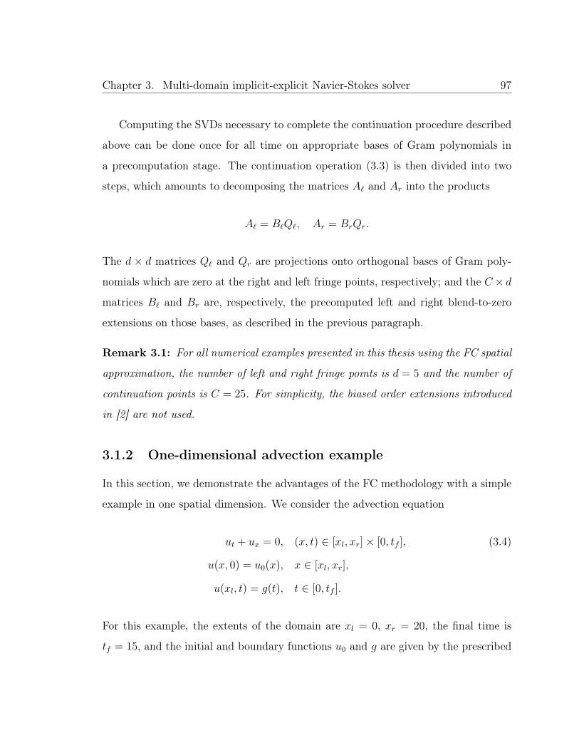
Chapter 3. Multi-domain implicit-explicit Navier-Stokes solver 97
Computing the SVDs necessary to complete the continuation procedure described
above can be done once for all time on appropriate bases of Gram polynomials in
a precomputation stage. The continuation operation (3.3) is then divided into two
steps, which amounts to decomposing the matrices A` and Ar into the products
A` = B`Q`, Ar = BrQr.
The d × d matrices Q` and Qr are projections onto orthogonal bases of Gram poly-
nomials which are zero at the right and left fringe points, respectively; and the C × dmatrices B` and Br are, respectively, the precomputed left and right blend-to-zero
extensions on those bases, as described in the previous paragraph.
Remark 3.1: For all numerical examples presented in this thesis using the FC spatial
approximation, the number of left and right fringe points is d = 5 and the number of
continuation points is C = 25. For simplicity, the biased order extensions introduced
in [2] are not used.
3.1.2 One-dimensional advection example
In this section, we demonstrate the advantages of the FC methodology with a simple
example in one spatial dimension. We consider the advection equation
ut + ux = 0, (x, t) ∈ [xl, xr]× [0, tf ], (3.4)
u(x, 0) = u0(x), x ∈ [xl, xr],
u(xl, t) = g(t), t ∈ [0, tf ].
For this example, the extents of the domain are xl = 0, xr = 20, the final time is
tf = 15, and the initial and boundary functions u0 and g are given by the prescribed
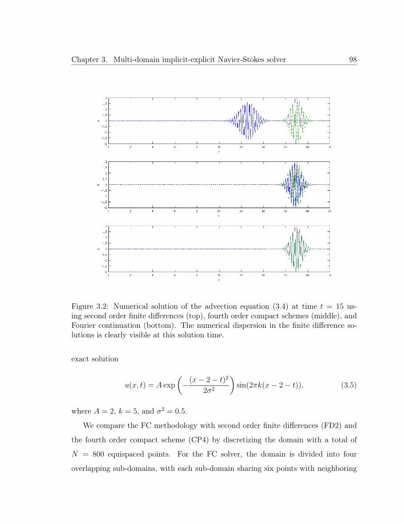
Chapter 3. Multi-domain implicit-explicit Navier-Stokes solver 98
Figure 3.2: Numerical solution of the advection equation (3.4) at time t = 15 us-ing second order finite differences (top), fourth order compact schemes (middle), andFourier continuation (bottom). The numerical dispersion in the finite difference so-lutions is clearly visible at this solution time.
exact solution
u(x, t) = A exp
(−(x− 2− t)2
2σ2
)sin(2πk(x− 2− t)), (3.5)
where A = 2, k = 5, and σ2 = 0.5.
We compare the FC methodology with second order finite differences (FD2) and
the fourth order compact scheme (CP4) by discretizing the domain with a total of
N = 800 equispaced points. For the FC solver, the domain is divided into four
overlapping sub-domains, with each sub-domain sharing six points with neighboring
Chapter 3. Multi-domain implicit-explicit Navier-Stokes solver 99
sub-domains. The solution is marched forward to the final time using the Adams-
Bashforth method of order four with ∆t = 0.1(xr − xl)/(N − 1) (see Sections 3.3
and 3.4 for description of the domain decomposition and time marching strategies).
The FC solver uses fourth order FC(Gram) continuation.
Figure 3.2 shows the solutions produced by each of the three solvers at the final
time tf = 15. Both finite difference solutions suffer from enough dispersion that the
error is essentially equal to the amplitude A of the exact solution. The FC solver,
on the other hand, has an error of 1.49 × 10⁻², using approximately 2.5 points per
wavelength. We also report the overall computation times (in seconds) for each of the
solvers (which were run on a single core): 0.464 (FC), 0.454 (CP4), 0.346 (FD2). This
example provides a powerful testimony to the strengths of the FC methodology for
wave-propagation problems, highlighting the near dispersionless-ness and efficiency
of the method.
3.1.3 Variable coefficient FC-ODE system solver
The implementation of the implicit component of the implicit-explicit solver presented
in this thesis requires solutions of one dimensional boundary-value ODE systems
discretized by the FC spatial approximation. To that end, we develop in this section
the FC-ODE system solver for general boundary-value problems that we use in the
Navier-Stokes solver.
Consider the ODE
Aq +B qx + C qxx = f (3.6)
on the interval x ∈ [0, 1], with general Robin boundary conditions
a q + b qx = g, x = 0 (3.7a)
c q + d qx = h, x = 1 (3.7b)
where q and f arem-dimensional vector-valued functions of x; A, B, and C arem×m

Chapter 3. Multi-domain implicit-explicit Navier-Stokes solver 100
matrix-valued functions of x; a, b, c, and d are m×m matrices; and g and h are m-
vectors. The matrices C, a, b, c, and d could have rows equal to zero—however, we
assume that each row of C is zero at x = 0 (respectively x = 1) if the corresponding
rows of a and b (c and d) are both zero (i.e., a boundary condition is supplied for
each row in equation 3.6 with second derivative terms).
Discretization of the interval into N equispaced points yields the vector- or matrix-
valued grid functions qi = q(xi), Ai = A(xi), etc. Let δx and δxx be the discrete
FC first and second derivative operators respectively. The system (3.6) is block-
decomposed, with the i-th interior block (i = 2, . . . , N − 1) given by
Aiqi +Bi
N∑j=1
(δx)ijqj + Ci
N∑j=1
(δxx)ijqj = fi. (3.8)
The non-zero rows of the boundary conditions (3.7) are used to replace the rows of
the discretized ODE for i = 1, N . In detail, let a superscript k denote the k-th row
of a vector or matrix. We introduce the modified matrices and vectors Ai, Bi and fi
(i = 1, N) given by
Ak1 =
Ak1 if ak = bk = 0
ak otherwiseAkN =
AkN if ck = dk = 0
ck otherwise
Bk1 =
Bk1 if ak = bk = 0
bk otherwiseBkN =
BkN if ck = dk = 0
dk otherwise
fk1 =
fk1 if ak = bk = 0
gk otherwisefkN =
fkN if ck = dk = 0
hk otherwise.
The first and N -th blocks of the discretized ODE system are then defined to be
Aiqi + Bi
N∑j=1
(δx)ijqj = fi, i = 1, N. (3.9)

Chapter 3. Multi-domain implicit-explicit Navier-Stokes solver 101
In general the linear system defined by equations (3.8) and (3.9) is full and non-
symmetric, so we use the GMRES iterative solver to invert the system [73]. A second
order finite difference solver is used to left precondition the system, which greatly
reduces the number of iterations needed for convergence [17]; cf. [10, Ch. 15.3].
The finite difference system is given by equations (3.8) and (3.9) with the discrete FC
derivative operators δx and δxx replaced by corresponding centered difference schemes
in the interior and a two-point one sided scheme at the boundary. The result is a
block-tridiagonal system which we invert efficiently using a block-LU decomposition.
The factorization need only be performed once per call of the GMRES solver.
Figure 3.3: One dimensional spatial convergence test of the variable coefficient FC-ODE solver for the system (3.10) with exact solution (3.11).
Figure 3.3 demonstrates the convergence of the solver for the model ODE system
Chapter 3. Multi-domain implicit-explicit Navier-Stokes solver 102
u+ ∆t
(u ux + Tx +
T
ρρx −
ν
ρuxx
)= f 1 (3.10a)
T + ∆t
(u Tx + T ux −
ν
ρTxx
)= f 2 (3.10b)
ρ+ ∆t (u ρx + ρ ux) = f 3 (3.10c)
in the domain x ∈ [0, 1], where ∆t = 0.01 and ν = 0.01 are constant, the functions
u, T , and ρ are given by
u = 1− 6esin(5x), T = log(3 + sin(6x)), ρ = 1 +1
2cos(4x2 + 2), (3.11)
and the right-hand side functions are chosen so that the exact solution is u = u,
T = T , ρ = ρ. Letting q = (u, T, ρ)T , the boundary conditions are given by (3.7)
with pseudorandom matrices
a =
0.71 0.39 0.19
0.51 0.71 0.06
0 0 0
b =
0.27 0.60 0.29
0.73 0.58 0.04
0 0 0
c =
0.87 0.57 0.20
0.19 0.41 0.51
0 0 0
d =
0.07 0.72 0.99
0.84 0.85 0.25
0 0 0
with the right-hand sides chosen to enforce the exact solution. Notice that no bound-
ary conditions are prescribed for ρ.
Remark 3.2: The paper [17] presents an alternative variable coefficient scalar FC-
ODE solver, which differs from the one presented here mainly in two respects: 1) It
solves for the particular and homogeneous solutions separately, using the homogeneous
solutions to correct the particular solution. This approach could be useful when solving

Chapter 3. Multi-domain implicit-explicit Navier-Stokes solver 103
many ODEs with the same coefficients and right-hand side but different boundary con-
ditions. However, due to the nonlinearity of the Navier-Stokes equations, the ODEs
we must solve have coefficients that change at each time step, and the approach in [17]
provides no significant advantage. 2) It uses high-order asymptotic matching for the
narrow boundary layers that occur in highly singularly perturbed ODEs, which were
necessary to ensure stability of the PDE solver for very small ∆t. These corrections
were found to be unnecessary for the stability of the Navier-Stokes solver for all time
discretizations we considered.
3.1.4 Filtering
Most high-order PDE solvers use some form of filtering or artificial viscosity to ensure
stability of the numerical solution, particularly for nonlinear problems. Previous FC-
based solvers have employed a Fourier-space exponential filter to great advantage [2,
3,35]. In detail, if the Fourier coefficients of the continued function are f ck , −Nc/2 ≤k ≤ Nc/2, then the filtered coefficients are given by
(f ck)filter = e−α| 2kNc |2p
f ck ,
where p is the order of the filter and α is a parameter such that the highest mode is
filtered to the level e−α.
Unfortunately, it is possible for the aforementioned filter to introduce relatively
large errors in the numerical solution. Qualitatively, the reason is that the continua-
tion portion of a function can have large peaks (sometimes several orders of magnitude
greater than the L∞ norm of the function in the physical domain) as well as the largest
spatial gradients. The exponential filter (or any Fourier-space filter for that matter)
will “smear” these peaks and gradients into the physical domain, leading to especially
large errors near the boundary.
The development of a suitable alternative filter is currently a topic of research.

Chapter 3. Multi-domain implicit-explicit Navier-Stokes solver 104
In the meantime, we use a Padé-type finite difference filter [39], which has been
shown to be effective in solving the Navier-Stokes equations in a finite-difference
context [38,90,91]. Given function values fi, the filtered function values fi sufficiently
far from the boundary satisfy
αfi−1 + fi + αfi+1 =n∑j=0
an2
(fi+j + fi−j),
where −0.5 < α ≤ 0.5 is a parameter determining the strength of the filter (with no
filtering at α = 0.5) and the n + 1 coefficients ai can be chosen so that the filtering
order is 2n. Reference [39] provides formulas for the coefficients, as well as similar
one-sided formulas for points near the boundaries.
In all our numerical results employing the FC methodology, we use a sixth order
filter (n = 3) with α = 0.3. Application of the filter is limited only to the physical
function values (ignoring the continuation region). The filter is applied to each line
of the computational domain in each dimension at the end of the time step.
3.2 Explicit time marching
Following [2], the Adams-Bashforth (AB) method [58, Ch. 3.9] is employed in all
domains requiring explicit time marching. Although the fourth order Runge-Kutta
(RK4) scheme is a popular choice for Navier-Stokes solvers, it is more expensive
than AB methods (requiring four evaluations of the right-hand side for every time
step) and proper treatment of boundary conditions at intermediate stages can be
problematic [1, 20].
In this thesis, AB methods of orders 2 to 4 are used, depending on the desired
order of time accuracy. Given the form of the PDE
Qt = P(Q, t),

Chapter 3. Multi-domain implicit-explicit Navier-Stokes solver 105
the AB scheme of order s for the approximate solution Qn+1 at time t = tn+1 is
Qn+1 = Qn + ∆ts−1∑j=0
bjP(Qn−j, tn−j), (3.12)
where the bj are the AB coefficients summarized in Table 3.1.
s b0 b1 b2 b3
1 1
2 32−1
2
3 2312−4
3512
4 5524−59
243724−3
8
Table 3.1: Coefficients for AB methods of orders s = 1, . . . , 4.
Explicit domains in all the numerical examples in this thesis use Dirichlet type
boundary conditions. Enforcement is accomplished by injecting the boundary values
at all boundary points at the end of each time step, as described in [2].
3.3 Domain decomposition
The decomposition of a general domain Ω proceeds by first dividing the space into
a set of larger overlapping logical rectangles Ωj such that Ω = ∪jΩj. These larger
patches are then divided into a set of sub-patches which share a layer of points with
neighboring sub-patches. In effect, each overset grid has one of two types of over-
lapping boundaries: 1) the overlap region is imperfect, in that one or more points
(generally all) do not correspond to any grid point in any neighboring patch, and 2)
all points in the boundary region are also grid points in a neighboring patch, result-
ing in a perfect overlap. Boundaries of the first type are referred to as interpolation
boundaries. They consist of sets of interpolation points, and they enable informa-
tion transfer from one grid to another by means of suitably high-order interpolation

Chapter 3. Multi-domain implicit-explicit Navier-Stokes solver 106
methods. The other kind of boundary, which we call an exchange boundary, does not
require interpolation.
Let p = (x∗, y∗, z∗) be an interpolation point in some domain Ωi. By definition,
p also lies in one or more other patches. Suppose Ωj is one such patch and let
q = (ξ∗, η∗, ζ∗) be the point in the computational domain of Ωj corresponding to
p—that is, x(ξ∗, η∗, ζ∗) = x∗ and similarly for the other coordinates. For Ωj to be
an acceptable donor patch, an m ×m ×m stencil of points (m is the stencil width,
resulting in an interpolation order of m) must be found such that the stencil includes
q in its interior, in such a way that no points in the interpolation stencil used are
themselves receivers of interpolation data from other patches. (Exchange points are
not excluded from being part of a donor stencil to an interpolation point). Of the
stencils satisfying these requirements, the one with q closest to its center is chosen. A
function is then interpolated in the computational domain using the tensor product
Lagrange interpolation formula.
Exchange points can be thought of as interpolation points where the point q is
itself one of the points in the donor stencil. Indeed, in such a case, the computed
interpolation weights will be zero for all but the coinciding point in the stencil, which
will be one. Thus, without loss of generality, in the remainder of this thesis “interpo-
lation” boundaries (points) will refer to both interpolation and exchange boundaries
(points). Differences in implementation will be noted where necessary.
In all our examples, a stencil width of m = 7 is employed, and each interpolation
boundary consists of a layer of two points deep, so that the overlap at an exchange
boundary is four points wide. Figure 3.4 illustrates the exchange data process in a
one-dimensional case.
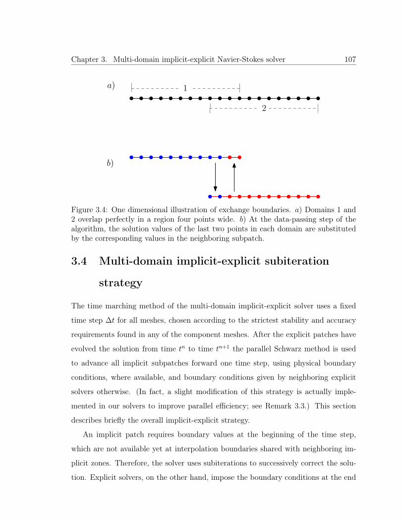
Chapter 3. Multi-domain implicit-explicit Navier-Stokes solver 107
1
2
a)
b)
Figure 3.4: One dimensional illustration of exchange boundaries. a) Domains 1 and2 overlap perfectly in a region four points wide. b) At the data-passing step of thealgorithm, the solution values of the last two points in each domain are substitutedby the corresponding values in the neighboring subpatch.
3.4 Multi-domain implicit-explicit subiteration
strategy
The time marching method of the multi-domain implicit-explicit solver uses a fixed
time step ∆t for all meshes, chosen according to the strictest stability and accuracy
requirements found in any of the component meshes. After the explicit patches have
evolved the solution from time tn to time tn+1 the parallel Schwarz method is used
to advance all implicit subpatches forward one time step, using physical boundary
conditions, where available, and boundary conditions given by neighboring explicit
solvers otherwise. (In fact, a slight modification of this strategy is actually imple-
mented in our solvers to improve parallel efficiency; see Remark 3.3.) This section
describes briefly the overall implicit-explicit strategy.
An implicit patch requires boundary values at the beginning of the time step,
which are not available yet at interpolation boundaries shared with neighboring im-
plicit zones. Therefore, the solver uses subiterations to successively correct the solu-
tion. Explicit solvers, on the other hand, impose the boundary conditions at the end

Chapter 3. Multi-domain implicit-explicit Navier-Stokes solver 108
of the time step, so no subiteration is required. The multi-domain implicit-explicit
subiteration algorithm ideally proceeds as follows:
1. All explicit zones are marched forward in time one time step.
2. Interpolation data from explicit zones is sent to neighboring zones.
3. All implicit zones are marched forward in time to obtain the subiteration solu-
tion.
4. After completion of each subiteration, interpolation data for boundary points is
exchanged between all implicit zones. (After the final subiteration, interpolation
data is sent to all explicit zones as well.)
5. The interpolated data received is used to set the boundary conditions at relevant
boundary points in all implicit zones, and steps 3 through 5 are repeated for
the specified number of subiterations.
Remark 3.3: Steps 1 and 3 could be performed in parallel provided approximate
(e.g., extrapolated) boundary conditions are used. Of course this cannot be carried
for all subiterations without leading to instability. But under certain circumstances
this strategy is recommended. For example, a processor assigned to an implicit zone
can proceed with the first subiteration in parallel with the explicit solves. In this
case, an initial approximation for the boundary conditions is obtained by means of
the temporal extrapolation formula (2.13). In practice this approach has provided an
effective parallelization methodology.
3.4.1 Convergence rate of the subiterations
This section presents analysis that explains the convergence properties of the implicit-
explicit iterations and, indeed, the particularly fast convergence that arises from
actual implementations of this approach in practice. This analysis shows that the

Chapter 3. Multi-domain implicit-explicit Navier-Stokes solver 109
error in subiteration solutions decreases exponentially fast with the size of the overlap
between sub-domains. Practical application of these results can be used to ensure that
a small number of subiterations suffice to meet a given accuracy requirement.
To effectively pursue this agenda we again restrict attention to the advection-
diffusion equation
ut + αux = βuxx
on the real line x ∈ R with u vanishing as x → ±∞. Overlapping patches are
simulated in this context by dividing the domain into two overlapping sub-domains,
Ω1 = (−∞, r) and Ω2 = (`,∞) with ` < r. Using for this example a semi-discrete
formalism (discrete in time and continuous in space), discretizing in time according
to the order-s BDF scheme and letting un denote the approximate solution at time
t = tn, we have the ODE boundary-value problem for un+1,
un+1 + b∆tLun+1 = fn ≡s−1∑j=0
ajun−j, (3.13)
where L = α ∂∂x− β ∂2
∂x2. The above equation is solved independently in each one of
the two subdomains according to the parallel Schwarz method. To that end, let vk1and vk2 be the approximate solutions of equation (3.13) in Ω1 and Ω2, respectively.
The subiteration procedure involves repeatedly solving
vk+11 + b∆tLvk+1
1 = fn in Ω1
vk+11 → 0 as x→ −∞
vk+11 (r) = vk2(r)
v01(r) = vr
vk+12 + b∆tLvk+1
2 = fn in Ω2
vk+12 → 0 as x→∞
vk+12 (`) = vk1(`)
v02(`) = v`,
(3.14)
where v` and vr are initial guesses for the value of un+1 at the points x = ` and r,
respectively. Letting ek1 = un+1 − vk1 and ek2 = un+1 − vk2 denote the error of the k-th

Chapter 3. Multi-domain implicit-explicit Navier-Stokes solver 110
subiteration in each subdomain, it is clear that the errors satisfy the homogeneous
versions of the same ODEs:
ek+11 + b∆tLek+1
1 = 0 in Ω1
ek+11 → 0 as x→ −∞
ek+11 (r) = ek2(r)
e01(r) = er
ek+12 + b∆tLek+1
2 = 0 in Ω2
ek+12 → 0 as x→∞
ek+12 (`) = ek1(`)
e02(`) = e`.
(3.15)
where e` = un+1(`)− v` and er = un+1(r)− vr.The two homogeneous solutions of the ODE are the exponentials
exp(λ1x), exp(−λ2x),
where
λ1 =
√α2
4β2+
1
βb∆t+
α
2β, λ2 =
√α2
4β2+
1
βb∆t− α
2β.
The positive exponential satisfies the boundary condition at −∞ in the left domain
Ω1 and the negative one satisfies the boundary condition at +∞ in Ω2. It follows
that the (k + 1)-th errors are given by
ek+11 = exp(−λ1(r − x)) ek2(r), ek+1
2 = exp(−λ2(x− `)) ek1(`). (3.16)
Evaluating each solution at the boundary point of the neighboring subdomain, we
obtain
ek+11 (`) = exp(−λ1δ) e
k2(r), ek+1
2 (r) = exp(−λ2δ) ek1(`), (3.17)
where δ = r−`. Using this recursive relation in equation (3.16), we obtain expressions

Chapter 3. Multi-domain implicit-explicit Navier-Stokes solver 111
for the error of the (k + 1)-th subiteration at the boundary of left domain
ek+11 (r) = exp(−λ2δ) e
k−11 (`)
= exp(−(λ1 + λ2)δ) ek−22 (r).
Letting
λ =1
2(λ1 + λ2) =
√α2
4β2+
1
βb∆t, (3.18)
it follows from an inductive argument that the error after k subiterations is given by
ek1(r) =
exp(−kλδ) er, k even
exp(−((k − 1)λ+ λ2)δ) e`, k odd(3.19)
The expression for the error at the boundary of the right domain, ek2(`), can be derived
similarly.
Using the even k expression in (3.19) (for simplicity), we can determine the ap-
proximate number of subiterations K that are necessary to reduce the error to the
level of O((∆t)s+1) in Ω1:
exp(−Kλδ) |er| ∼ (∆t)s+1
=⇒ K ≈ −1
λδln
((∆t)s+1
|er|
).
The corresponding estimate in Ω2 uses e` instead of er. With temporal extrapolation
of order s, the initial boundary conditions can be chosen so that the initial errors
will be e` = O((∆t)s) and er = O((∆t)s). Therefore the approximate number of
subiterations necessary for an error tolerance of order (∆t)s+1 is
K ≈ − ln(∆t)
λδ. (3.20)

Chapter 3. Multi-domain implicit-explicit Navier-Stokes solver 112
Consideration of the two terms under the radical in equation (3.18),
α2
4β2and
1
βb∆t,
under certain physical regimes allows us to provide even simpler specialized expres-
sions. Indeed, in the “convection dominated” regime the second term is small com-
pared to the first and we thus have
β
α2 ∆t 1 =⇒ λ ∼ α
2β.
This is applicable to the case of high Reynolds number flow with a relatively large
time step. The “diffusion dominated” case is given by the other extreme:
β
α2 ∆t 1 =⇒ λ ∼ 1√
βb∆t.
The revised estimates for the necessary number of subiterations in each of these cases
is
K ≈
2β
α δ| ln ∆t| convection dominated
√βb∆t
δ| ln ∆t| diffusion dominated.
(3.21)
The results of the analysis for the linearized one-dimensional Navier-Stokes equa-
tions presented in Section 2.4.2 together with the estimate above are used to provide
specific suggestions for the number of iterations needed under subsonic flow of a
compressible gas. In this context, the viscosity β scales like Re−1 and the advec-
tion velocity α scales like either the fluid velocity |u| for convective-type waves (i.e.,
vorticity and entropy waves) or |u| + Ma−1 for acoustic waves. Thus, the number
of iterations necessary to eliminate errors associated with convection, acoustics and

Chapter 3. Multi-domain implicit-explicit Navier-Stokes solver 113
diffusion satisfy
K ≈
2| ln ∆t||u|Re δ
(vorticity and entropy waves)
2| ln ∆t|(|u|+ Ma−1) Re δ
(acoustic waves)
1
δ
√b∆t
Re| ln ∆t| (diffusion).
(3.22)
For the overset method employed in this thesis, the amount of overlap will gener-
ally be δ ≈ mh for some number m = O(1) and spatial mesh size h. If h is chosen
to be on the order of Re−1, for example, equation (3.22) indicates that the number
of subiterations necessary to resolve wave phenomena will be O(| ln ∆t|). Using the
same discretization, diffusive phenomena will require O(√
∆tRe| ln ∆t|) subiterationsto reach the level of the truncation error.
3.5 Parallelization
The overset mesh framework together with the parallel Schwarz subiteration strat-
egy naturally lead to a parallel implementation in a distributed computing environ-
ment. An efficient implementation should divide the workload among all processors
as equally as possible. Details in this regard for explicit FC solvers is well documented
in [2,3]. As the solver presented in this thesis is the first implicit and implicit-explicit
multi-domain FC solver, additional details need to be presented. To that end, this
section provides heuristics for decomposing a domain to maximize efficiency, as well
as an investigation of the computational cost of the implicit multi-domain solver.
3.5.1 Implicit multi-domain load balancing
The present load-balancing algorithm is based on the ones presented in [2, 3]. Given
a set of implicit patches ΩIj, j = 1, . . . ,MI and a number of target zones ptotal, the

Chapter 3. Multi-domain implicit-explicit Navier-Stokes solver 114
target number of sub-zones assigned to an implicit patch ΩIj is
pIj =N jξN
jηN
jζ
MI∑l=1
N lξN
lηN
lζ
ptotal
(rounded to the nearest integer), where N jξ , N
jη , N
jζ are the numbers of discretization
points in each dimension. The partitioning of a patch into subpatches is performed
in such a way that, for each subpatch, the number of discretization points in each
direction is approximately equal. If p is the number of target zones assigned to a
patch, then the number of partitions in the ξ direction is given by
sξ = Nξ
(p
NξNηNζ
) 13
,
rounded to the nearest integer greater than or equal to one. Similar formulas hold
for the number of partitions in the η and ζ directions.
Note that the method of sub-zone distribution and partitioning described above
could result in a number of subpatches different from the target number of zones. In
practice the difference is negligible and the method produces satisfactory results for
our purposes.
3.5.2 Implicit multi-domain performance
In this section, we present the results of various computational experiments of the
parallel implicit multi-domain solver in a distributed computing environment. All
results were obtained on a Poweredge cluster with Inifiniband networking, consisting
of 32 compute nodes, each of which has two eight-core Intel Xeon E5-2665 processors
(for up to 32 threads per node with Intel Hyper-threading) and 64 GB of memory.
In [2,3], the authors quantified the cost of the explicit FC solvers using the number
S of seconds required per processor to advance one million unknowns forward one time

Chapter 3. Multi-domain implicit-explicit Navier-Stokes solver 115
step, which, for our Navier-Stokes solver, is given by the formula
S =(# of processors)× (total compute time per step)× 106
(d+ 2)× (# of discretization points), (3.23)
where the factor of d + 2 in the denominator is the size of the vector of unknowns
Q in d = 2 and 3 spatial dimensions. The present explicit FC-based Navier-Stokes
solver enjoys approximately the same efficiency as the solvers in those contributions—
namely,
S ≈ 1.6 sec. (for explicit solvers). (3.24)
To test the efficiency of the parallel implicit algorithm, we use a smaller version of
the mesh described in Section 4.2.2 of the following chapter, which is used for three
dimensional tests of flow past a sphere. In this example, the limits of the domain are
[−3, 3] in each dimension, with the extent of the spherical-like curvilinear patches the
same as in Section 4.2.2. The mesh spacing in the Cartesian patches is a constant
value h, while the radial spacing in the curvilinear patches is h/10 near the surface
of the sphere and h at the outer edge of the patch. The initial conditions and source
terms are the same as in the tests of flow past a sphere.
hmax 0.06 0.048 0.04# grid points 2,045,990 3,817,125 6,372,454
# sub-domains 104 194 104 194 294S (1 sub-iter.) 36.8 33.4 33.9 30.7 32.6S (2 sub-iter.) 54.3 58.9 53.4 51.6 55.3S (3 sub-iter.) 86.6 78.8 74.4 74.9 77.0
Table 3.2: Number of seconds S needed per processor for the parallel implicit algo-rithm to advance one million unknowns forward one time step, with various numbersof discretization points, sub-domains, and subiterations.
Table 3.2 reports the value of S for the BDF2-ADI solver on the composite mesh
for various values of h, sub-domain partitionings, and number of sub-iterations. In
these tests, the Mach number was 0.8, the Reynolds number was 103, and the GMRES
Chapter 3. Multi-domain implicit-explicit Navier-Stokes solver 116
residual tolerance was set to 10−6. The solver was run for a total of 20 time steps
with ∆t = 10−3. The results show that S is approximately constant for each fixed
number of sub-iterations, which corresponds to approximately linear parallel scaling
of the implicit algorithm.
We can also use the data in Table 3.2 to compare the computational costs of the
explicit and implicit algorithms. For one sub-iteration, the implicit solver is about
twenty times more expensive than the explicit solver—which is reasonable if, for
example, each ADI sweep in each of the three spatial dimensions takes about six or
seven GMRES iterations to converge. Two sub-iterations of the implicit solver (which
we use in our numerical examples) is about thirty-five times more expensive than the
explicit solver. This suggests that the implicit solver is most advantageous when the
time step ∆t required by the explicit solver for stability is about 35 times smaller
than that required by the implicit solver.
Remark 3.4: In the context of the implicit solver presented in this thesis, many
factors can affect the convergence rate of GMRES—such as the size of the time step
∆t, the physical parameters (particularly Reynolds and Mach numbers), how well
the solution is spatially resolved, the accuracy order of the temporal discretization,
boundary conditions, etc.—but we have found the most influential factors to be the
time step ∆t and the Reyolds number. As ∆t → 0, the operator to be inverted is
asymptotic to the identity, leading to faster convergence. On the other hand, large
Reynolds number makes the operator more singularly perturbed (i.e., the coefficients
of the second derivatives become smaller), and the spectrum of the centered finite
difference preconditioner does not approximate the spectrum of the actual operator
well (see [10, Ch. 15.3]). Nevertheless, we have observed that the performance results
given in Table 3.2 are fairly generic.

Chapter 4. Numerical results 117
Chapter 4
Numerical results
This chapter presents a variety of numerical examples for the BDF-ADI solver in single
domains, as well as the full multi-domain solver. The main purpose of the simulations
is to showcase the stability and accuracy of the proposed methodologies. Once again
we emphasize that these results represent the first numerical demonstrations of high-
order time-accuracy for any ADI solver of the compressible Navier-Stokes equations.
Unless otherwise indicated, all simulations use the parameter values Pr = 0.71
and γ = 1.4, and the (non-dimensional) viscosity and thermal conductivity are given
by Sutherland’s law [95, pp. 28–30]
κ(T ) =1 + SκT + Sκ
T 3/2 and µ(T ) =1 + SµT + Sµ
T 3/2,
where Sκ and Sµ are the non-dimensionalized Sutherland constants, which, for defi-
niteness, are set to Sκ = Sµ = 0.3.
4.1 The BDF-ADI solver in single domains
The focus of this section is single domain, single core runs of the BDF-ADI solvers
introduced in this thesis for two- and three-dimensional spatial domains and for orders
s with 2 ≤ s ≤ 6. In particular, some of these results demonstrate that the proposed
solvers do enjoy the claimed spatial and temporal orders of accuracy, while other

Chapter 4. Numerical results 118
examples demonstrate the methods’ stability properties and general applicability.
All of the numerical examples were obtained from runs on either a single core of an
Intel Core i5-2520M processor with 4 GB of memory, or a single core of an Intel Xeon
X5650 processor with 24 GB of memory.
We emphasize that in this section only, Chebyshev and Fourier spectral discretiza-
tions in space are used (as opposed to the FC method used in the full multi-domain
solver). The reasons are twofold: First, the BDF-ADI algorithm was developed inde-
pendently of any spatial approximation, and a goal of this thesis is to demonstrate
wider applicability of the scheme. Second, the Chebyshev approximation is known for
the O(1/N2) clustering of points near the boundaries of the domain, and we demon-
strate that this does not pose a challenge to the quasi-unconditional stability of the
solvers.
4.1.1 Convergence in Cartesian domains
Figure 4.1: Convergence of the two-dimensional BDF-ADI solvers of orders s =2, . . . , 6 in a Cartesian square.

Chapter 4. Numerical results 119
Figure 4.2: Convergence of the three-dimensional BDF-ADI solvers of orders s =2, . . . , 6 in a Cartesian cube.
Using the method of manufactured solutions (MMS), our first set of examples
demonstrates that the proposed solvers achieve the expected temporal order of con-
vergence in two- and three-dimensional problems. According to the MMS strategy, an
arbitrary solution Q is prescribed, and a source term is added to the right-hand side
of equations (2.5) or (2.6), as appropriate, in such a way that the proposed solution
actually satisfies the equation. For this set of examples we use the manufactured
solution
Qj(x, t) = αj + βj sin(λjt+ φj,t)d∏i=1
sin(2π xi + φj,xi) (4.1)
(d = 2, 3), where Qj is the jth component of the solution vector and where αj, βj, λj,
φj,xi are constants. The parameter values we use for the two- and three-dimensional
solutions are given in Tables 4.1 and 4.2, respectively. The test geometry in this
context is a Cartesian box of side-length equal to one. Only the velocity components
and temperature T are prescribed at the boundary according to the manufactured

Chapter 4. Numerical results 120
solution; the boundary values of the density are obtained as part of the solution
process, as described in Section 2.5.2. The Reynolds number and Mach number in
these examples are taken to equal Re = 103 and Ma = 0.85. The second- through
sixth-order convergence of the BDF-ADI methods is demonstrated in Figures 4.1
and 4.2. All tests were run to a final time of t = 1.0, with the L∞ error measured
against the manufactured solution at that time. In the tests for the methods of orders
four, five and six, the temporal frequency of the manufactured solution was increased,
so that the errors associated with the temporal discretization are large compared to
the spatial discretization errors. This allows the convergence slopes to be observed
at moderate ∆t without requiring very fine spatial resolution.
Qj αj βj λj φj,t φj,x φj,yu 0 1 6 (37) 1 0 0v 0 1 6 (37) 2 0 0ρ 1 0.2 6 (37) 3 0.5 1.5T 1 0.2 6 (37) 4 1 2
Table 4.1: Parameters for two-dimensional manufactured solution. The temporalfrequencies λj not in parentheses are the ones used in the convergence tests for themethods of orders s = 2, 3, while the ones in parentheses are those used in the orders = 4, 5, 6 tests.
Qj αj βj λj φj,t φj,x φj,y φj,zu 0 1 7 (37) -1 0 0 0v 0 1 7 (37) -2 0 0 0w 0 1 7 (37) -3 0 0 0ρ 1 0.2 7 (37) -4 4 7 14T 1 0.2 7 (37) -5 5 6 15
Table 4.2: Parameters for three-dimensional manufactured solution. The temporalfrequencies λj not in parentheses are the ones used in the convergence tests for themethods of orders s = 2, 3, while the ones in parentheses are those used in the orders = 4, 5, 6 tests.
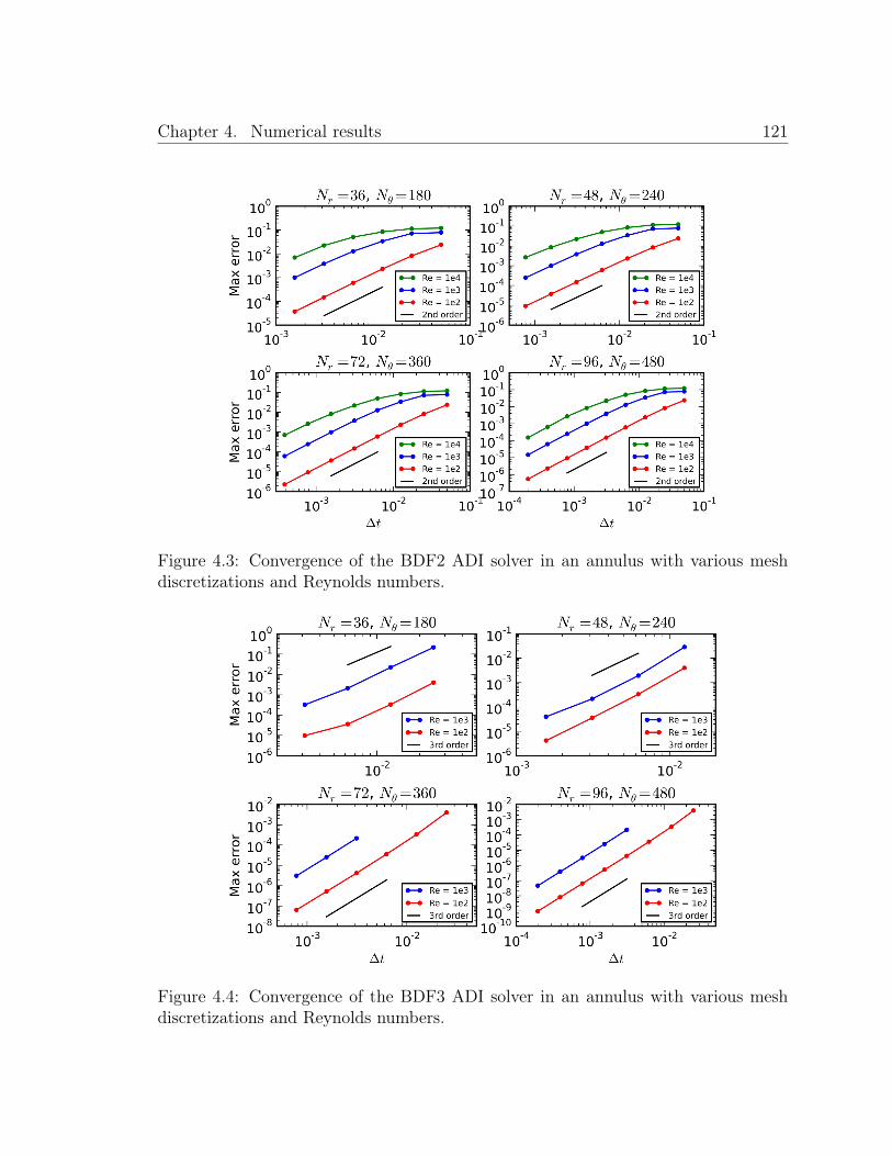
Chapter 4. Numerical results 121
Figure 4.3: Convergence of the BDF2 ADI solver in an annulus with various meshdiscretizations and Reynolds numbers.
Figure 4.4: Convergence of the BDF3 ADI solver in an annulus with various meshdiscretizations and Reynolds numbers.
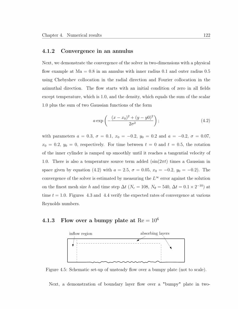
Chapter 4. Numerical results 122
4.1.2 Convergence in an annulus
Next, we demonstrate the convergence of the solver in two-dimensions with a physical
flow example at Ma = 0.8 in an annulus with inner radius 0.1 and outer radius 0.5
using Chebyshev collocation in the radial direction and Fourier collocation in the
azimuthal direction. The flow starts with an initial condition of zero in all fields
except temperature, which is 1.0, and the density, which equals the sum of the scalar
1.0 plus the sum of two Gaussian functions of the form
a exp
(−(x− x0)2 + (y − y0)2
2σ2
); (4.2)
with parameters a = 0.3, σ = 0.1, x0 = −0.2, y0 = 0.2 and a = −0.2, σ = 0.07,
x0 = 0.2, y0 = 0, respectively. For time between t = 0 and t = 0.5, the rotation
of the inner cylinder is ramped up smoothly until it reaches a tangential velocity of
1.0. There is also a temperature source term added (sin(2πt) times a Gaussian in
space given by equation (4.2) with a = 2.5, σ = 0.05, x0 = −0.2, y0 = −0.2). The
convergence of the solver is estimated by measuring the L∞ error against the solution
on the finest mesh size h and time step ∆t (Nr = 108, Nθ = 540, ∆t = 0.1× 2−10) at
time t = 1.0. Figures 4.3 and 4.4 verify the expected rates of convergence at various
Reynolds numbers.
4.1.3 Flow over a bumpy plate at Re = 106
absorbing layersinflow region
Figure 4.5: Schematic set-up of unsteady flow over a bumpy plate (not to scale).
Next, a demonstration of boundary layer flow over a "bumpy" plate in two-

Chapter 4. Numerical results 123
dimensions at high Reynolds number is given. Here the domain is such that the
left edge is xl = 1, the right edge is xr = 4, the top edge is yt = 0.2, and the bottom
edge is
yb(x) = exp
(−(x− 2.5
1.2
)12)
4∑m=1
am sin(cmx),
where the coefficients are given by am = 5 × 10⁻⁴, 8 × 10⁻⁴, 6 × 10⁻⁴, 4 × 10⁻⁴ and
cm = 300, 207, 161, 124. The interior points of the domain are generated by means of
transfinite interpolation [42]. A total of 1536 (resp. 96) Chebyshev collocation points
were used in the horizontal direction (resp. in the vertical direction). A schematic
illustration of the set-up is provided in Figure 4.5.
To initialize the flow and impose boundary conditions, we first obtain the solution
of the compressible boundary layer equations. Here we provide a brief overview of
their derivation; a more detailed discussion can be found in, e.g., [95, Ch. 7]. For
simplicity, we assume the viscosity and thermal conductivity are linear functions of
temperature (µ(T ) = κ(T ) = T ) and the Prandtl number is Pr = 1. The x and
y directions are tangent and normal to the boundary respectively, and we take the
free-stream values as y →∞ to be u∞ = 1, v∞ = 0, T∞ = 1, ρ∞ = 1.
The boundary layer equations are obtained by transforming the steady (Qt = 0)
two-dimensional Navier-Stokes equations (2.3) with the change of variable y = δY ,
where δ = Re1/2 is the characteristic length scale of the boundary layer. Furthermore,
the solution components are assumed to be perturbations of the free-stream values
of the form u = u∞ + δu1, v = δv1, T = T∞ + δT1, ρ = ρ∞ + δρ1, which leads to a
set of equations for the inner solutions (terms with subscript 1). Using the similarity
variable η = η(x−1/2Y ) together with the Howarth transformation [49], we obtain the
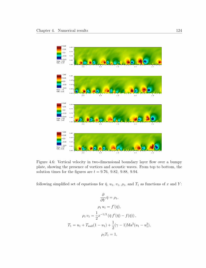
Chapter 4. Numerical results 124
Figure 4.6: Vertical velocity in two-dimensional boundary layer flow over a bumpyplate, showing the presence of vortices and acoustic waves. From top to bottom, thesolution times for the figures are t = 9.76, 9.82, 9.88, 9.94.
following simplified set of equations for η, u1, v1, ρ1, and T1 as functions of x and Y :
∂
∂Yη = ρ1,
ρ1 u1 = f ′(η),
ρ1 v1 =1
2x−1/2 (η f ′(η)− f(η)) ,
T1 = u1 + Twall(1− u1) +1
2(γ − 1)Ma2(u1 − u2
1),
ρ1T1 = 1,

Chapter 4. Numerical results 125
where Twall is the temperature at the wall and f is the solution of the Blasius equation
f ′′′ +1
2f f ′ = 0,
f(0) = f ′(0) = 0,
f ′(η)→ 1 as η →∞.
The similarity variable η is obtained by eliminating the other unknowns and using
a Newton-Kantorovich iterative solver [10, App. C] with initial guess computed by
standard fourth order Runge-Kutta. The rest of the unknowns can then be obtained
explicitly from the above relations. The solution Qref of the boundary layer equations
is used to provide the initial condition and boundary conditions at inflow and in the
absorbing layers of the computational domain.
The boundary conditions for this example are as shown in Figure 4.5—no-slip
conditions are imposed on the bottom boundary (uwall = 0 and Twall = 1), an ab-
sorbing layer of thickness 0.05 is used at the top of the domain, another absorbing
layer of thickness 0.5 is used at right, and inflow conditions are imposed in a region
of thickness 0.1 at the left. For each absorbing layer, a term of the form σ(ξ, η)Qref
is added to the right-hand side of the PDE (2.6) and σI is added to the matrix M0,
where I is the identity. The variable coefficient σ is given by
σ(ξ, η) = A
(1− ψ
(d(ξ, η)
L
))(4.3)
where A is the absorption factor, L is the width of the layer, d(ξ, η) is the distance
to the boundary in question, and the function ψ is given by
ψ(x) =
0, x ≤ 0
1, x ≥ 1[1 + exp
(1x− 1
1−x
)]−1, 0 < x < 1.
(4.4)

Chapter 4. Numerical results 126
For the top boundary we use A = 50, L = 0.05, and for the right boundary we use
A = 20, L = 0.5. The boundary layer solution Qref is imposed in the inflow region.
Figure 4.6 shows the vertical velocity for various times, with Re = 106, Ma = 0.85,
and ∆t = 10−3. With this discretization (∆xmin = 3.1×10⁻⁶ and ∆ymin = 5.4×10⁻⁵),
an explicit solver would require a prohibitively small time step (. 10−6) for stability.
4.1.4 Wall bounded Taylor-Couette flow
Figure 4.7: Geometry of Taylor-Couette flow. The fluid is confined to the regionbetween two cylinders of radii ri and ro, and two planes separated by a length h. Theinner cylinder rotates with speed Ui, while all other boundaries remain stationary.
We also verify the three-dimensional solver by simulation of Taylor-Couette flow,
which is flow of a fluid between two concentric rotating cylinders. Most studies of
Taylor-Couette flow deal with incompressible fluids, but the dynamics for subsonic
compressible gases are similar, as shown in [52, 65]. The geometry (illustrated in
Figure 4.7) is defined by the inner radius ri, outer radius ro, and height h. In what
follows, we consider only the case where the inner cylinder rotates and the outer
cylinder together with the top and bottom walls are stationary. In this case, the
Reynolds number Re is defined with respect to the velocity of the inner cylinder.
The small aspect ratio regime (Γ = hro−ri ≈ 1 or less) has been extensively studied
both numerically and experimentally (in the incompressible case)—in part because of
the property that two or more stable flows can exist for the same values of the system

Chapter 4. Numerical results 127
Figure 4.8: Profiles of the (a) azimuthal velocity, (b) vertical velocity, and (c) az-imuthal component of vorticity in small-aspect-ratio Taylor-Couette flow at Ma = 0.2and Re = 700. The top (bottom) row has the profiles of the two-cell (one-cell) stablemode.
parameters Γ, Re, ro, ri [66, 71]. For Γ = 1 and radius ratio ri/ro = 0.5, there is
only one stable flow at small Re, which is characterized by two axisymmetric toroidal
vortices, one on top of the other, as pictured in the upper frame of Figure 4.8 (c). At
about Re ≈ 133, this mode becomes unstable. The stable mode is then characterized
by a single large axisymmetric toroidal vortex in the center and a smaller one in the
inner upper corner, as shown in the lower frame of Figure 4.8 (c). Both modes are
stable in the range 603 . Re . 786.
Starting from the same initial condition (zero velocity, density and temperature
equal to 1.0) and ending at the same final inner cylinder rotation at Re = 700 and
Ma = 0.2, we arrive at both stable modes. For the two-cell mode, the inner cylinder
velocity as a function of time is given by
Ui(t) = ψ
(t
160
),
where ψ is defined in (4.4). To demonstrate the one-cell mode, the cylinder velocity

Chapter 4. Numerical results 128
is given by
Ui(t) = 0.4ψ
(t
10
)+ 0.6ψ
(t− 150
150
).
The domain is discretized using 48 Chebyshev collocation points in the radial and
z directions and 64 Fourier collocation points in the azimuthal direction. No-slip
isothermal boundary conditions are used on all walls, with the axial velocity on the
top and bottom boundaries given by
uθ(r, t) = exp
(−(
2√
Re(r − ri))2)Ui(t).
The time discretization for both simulations was set at ∆t = 0.02 and simulations were
stopped at t = 400. At Ma = 0.2, there is less than 0.5% deviation in the density from
the initial condition ρ = T = 1 throughout the simulations. The presence of corners
in the geometry undoubtedly reduces the accuracy of the solutions; nevertheless,
Figure 4.8 shows both modes at t = 300, which compares well to the experimental
and numerical results in the literature for the incompressible case [66,71]—as it should
given the low value of the Mach number considered.
4.2 Multi-domain implicit-explicit examples
This section showcases the full multi-domain implicit-explicit algorithm with one
example each in two and three spatial dimensions. These results were obtained on
the cluster described in Section 3.5.2.
4.2.1 Unsteady flow past a cylinder
This section presents numerical results for the problem of flow past a cylinder in two
spatial dimensions with Re = 200. At higher values of the Reynolds number three-
dimensional effects become important thus reducing the relevance of two-dimensional
simulations.

Chapter 4. Numerical results 129
Figure 4.9: Two close-ups of the mesh used in the numerical experiments of flow pasta cylinder. The bottom figure shows the clustering of points near the cylinder surfaceto spatially resolve the boundary layer.
The two-dimensional cross-section is the region inside the rectangle [−8, 24] ×[−8, 8] and outside a circle of radius rc = 0.5 centered at the origin. This region is
divided into 13 overlapping patches: four curvilinear annular-like sections surrounding
the cylinder and nine rectangular patches away from the cylinder. Our approach to
generation of the curvilinear meshes is discussed in Appendix B. Figure 4.9 shows a
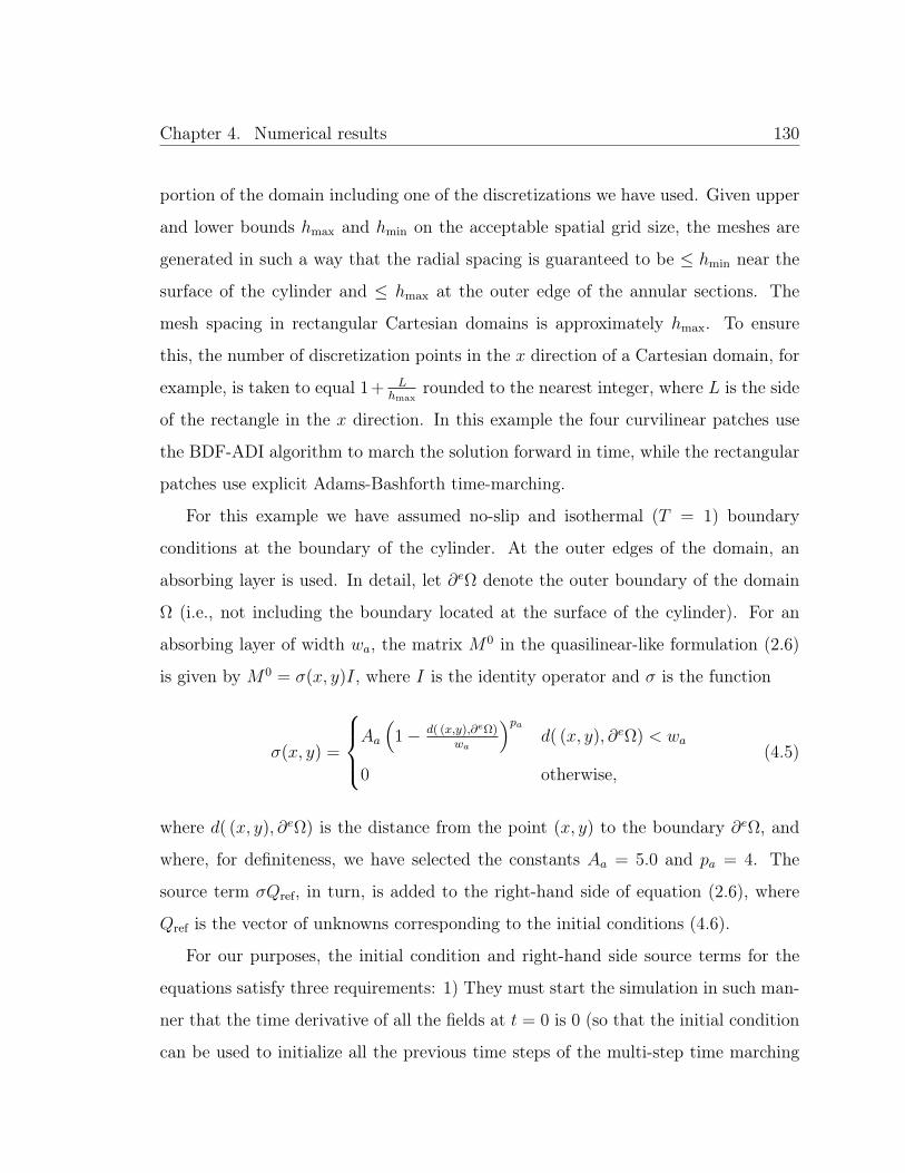
Chapter 4. Numerical results 130
portion of the domain including one of the discretizations we have used. Given upper
and lower bounds hmax and hmin on the acceptable spatial grid size, the meshes are
generated in such a way that the radial spacing is guaranteed to be ≤ hmin near the
surface of the cylinder and ≤ hmax at the outer edge of the annular sections. The
mesh spacing in rectangular Cartesian domains is approximately hmax. To ensure
this, the number of discretization points in the x direction of a Cartesian domain, for
example, is taken to equal 1+ Lhmax
rounded to the nearest integer, where L is the side
of the rectangle in the x direction. In this example the four curvilinear patches use
the BDF-ADI algorithm to march the solution forward in time, while the rectangular
patches use explicit Adams-Bashforth time-marching.
For this example we have assumed no-slip and isothermal (T = 1) boundary
conditions at the boundary of the cylinder. At the outer edges of the domain, an
absorbing layer is used. In detail, let ∂eΩ denote the outer boundary of the domain
Ω (i.e., not including the boundary located at the surface of the cylinder). For an
absorbing layer of width wa, the matrix M0 in the quasilinear-like formulation (2.6)
is given by M0 = σ(x, y)I, where I is the identity operator and σ is the function
σ(x, y) =
Aa(
1− d( (x,y),∂eΩ)wa
)pad( (x, y), ∂eΩ) < wa
0 otherwise,(4.5)
where d( (x, y), ∂eΩ) is the distance from the point (x, y) to the boundary ∂eΩ, and
where, for definiteness, we have selected the constants Aa = 5.0 and pa = 4. The
source term σQref, in turn, is added to the right-hand side of equation (2.6), where
Qref is the vector of unknowns corresponding to the initial conditions (4.6).
For our purposes, the initial condition and right-hand side source terms for the
equations satisfy three requirements: 1) They must start the simulation in such man-
ner that the time derivative of all the fields at t = 0 is 0 (so that the initial condition
can be used to initialize all the previous time steps of the multi-step time marching

Chapter 4. Numerical results 131
schemes, without reducing the temporal order of accuracy), 2) they reduce the amount
of time it takes for the solution to settle into the periodic vortex shedding mode by
breaking the symmetry of the flow early on and 3) they satisfy the no-slip, isothermal
boundary condition at the surface of the cylinder and the free stream conditions in
the absorbing layer for all times t.
Figure 4.10: Temporal convergence of the solver for flow past a cylinder at timet = 1.0, with Re = 200 and Ma = 0.8.
In view of these goals the flow is initialized with the radially symmetric fields
ρ = T = 1, v = 0, u = u0ψs(r − rc), (4.6)
where u0 is the freestream velocity and ψs is the smooth step function
ψs(x) =
0 x ≤ 0(1 + exp
(1x− 1
1−x
))−10 < x < 1
1 x ≥ 1.
(4.7)
This initial condition satisfies the no-slip and isothermal conditions at the surface of
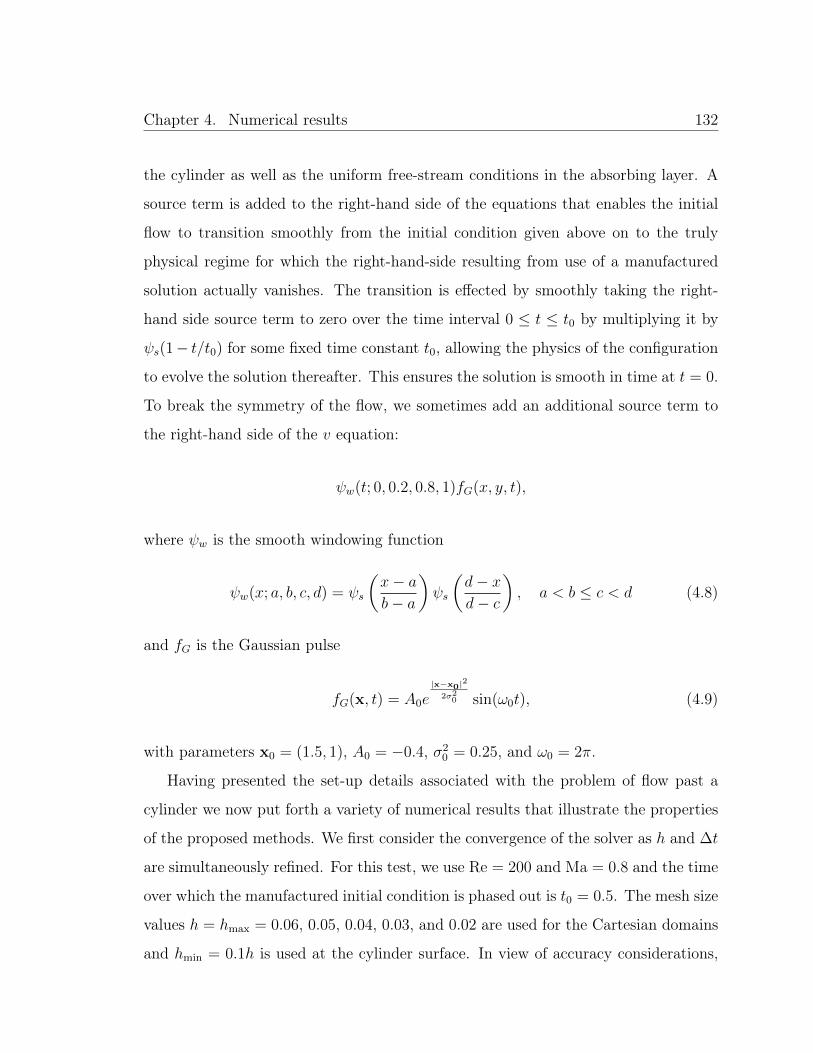
Chapter 4. Numerical results 132
the cylinder as well as the uniform free-stream conditions in the absorbing layer. A
source term is added to the right-hand side of the equations that enables the initial
flow to transition smoothly from the initial condition given above on to the truly
physical regime for which the right-hand-side resulting from use of a manufactured
solution actually vanishes. The transition is effected by smoothly taking the right-
hand side source term to zero over the time interval 0 ≤ t ≤ t0 by multiplying it by
ψs(1− t/t0) for some fixed time constant t0, allowing the physics of the configuration
to evolve the solution thereafter. This ensures the solution is smooth in time at t = 0.
To break the symmetry of the flow, we sometimes add an additional source term to
the right-hand side of the v equation:
ψw(t; 0, 0.2, 0.8, 1)fG(x, y, t),
where ψw is the smooth windowing function
ψw(x; a, b, c, d) = ψs
(x− ab− a
)ψs
(d− xd− c
), a < b ≤ c < d (4.8)
and fG is the Gaussian pulse
fG(x, t) = A0e|x−x0|
2
2σ20 sin(ω0t), (4.9)
with parameters x0 = (1.5, 1), A0 = −0.4, σ20 = 0.25, and ω0 = 2π.
Having presented the set-up details associated with the problem of flow past a
cylinder we now put forth a variety of numerical results that illustrate the properties
of the proposed methods. We first consider the convergence of the solver as h and ∆t
are simultaneously refined. For this test, we use Re = 200 and Ma = 0.8 and the time
over which the manufactured initial condition is phased out is t0 = 0.5. The mesh size
values h = hmax = 0.06, 0.05, 0.04, 0.03, and 0.02 are used for the Cartesian domains
and hmin = 0.1h is used at the cylinder surface. In view of accuracy considerations,
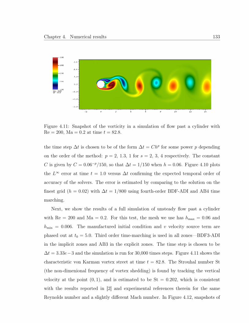
Chapter 4. Numerical results 133
Figure 4.11: Snapshot of the vorticity in a simulation of flow past a cylinder withRe = 200, Ma = 0.2 at time t = 82.8.
the time step ∆t is chosen to be of the form ∆t = Chp for some power p depending
on the order of the method: p = 2, 1.3, 1 for s = 2, 3, 4 respectively. The constant
C is given by C = 0.06−p/150, so that ∆t = 1/150 when h = 0.06. Figure 4.10 plots
the L∞ error at time t = 1.0 versus ∆t confirming the expected temporal order of
accuracy of the solvers. The error is estimated by comparing to the solution on the
finest grid (h = 0.02) with ∆t = 1/800 using fourth-order BDF-ADI and AB4 time
marching.
Next, we show the results of a full simulation of unsteady flow past a cylinder
with Re = 200 and Ma = 0.2. For this test, the mesh we use has hmax = 0.06 and
hmin = 0.006. The manufactured initial condition and v velocity source term are
phased out at t0 = 5.0. Third order time-marching is used in all zones—BDF3-ADI
in the implicit zones and AB3 in the explicit zones. The time step is chosen to be
∆t = 3.33e−3 and the simulation is run for 30,000 times steps. Figure 4.11 shows the
characteristic von Karman vortex street at time t = 82.8. The Strouhal number St
(the non-dimenional frequency of vortex shedding) is found by tracking the vertical
velocity at the point (0, 1), and is estimated to be St = 0.202, which is consistent
with the results reported in [2] and experimental references therein for the same
Reynolds number and a slightly different Mach number. In Figure 4.12, snapshots of

Chapter 4. Numerical results 134
t = 70.8 t = 71.6
t = 72.4 t = 73.2
Figure 4.12: Time evolution of streamlines in flow past a cylinder at Re = 200 andMa = 0.2. Darker shading of the streamline corresponds to a higher magnitude ofthe velocity at that point.
the streamlines near the cylinder show the time evolution of vortex shedding.

Chapter 4. Numerical results 135
4.2.2 Unsteady flow past a sphere
In this section, we present the results of three-dimensional flow past a sphere. The
domain is the region inside the box (x, y, z) ∈ [−4, 14]× [−4, 4]× [−4, 4] and outside
the sphere of radius rs = 0.5 centered at the origin. This region is divided into 12
larger overlapping patches: two curvilinear patches forming a modified “Yin-Yang”
mesh [51] surrounding the sphere and ten Cartesian patches away from the sphere.
Generation of the curvilinear meshes is discussed in Appendix B. The BDF-ADI
method is used in the curvilinear patches and explicit AB time marching is used in
all Cartesian patches. Given values hs, hc, hf , and hu, to be selected in what follows,
meshes are generated in such a way that the radial spacing is hs near the surface of the
sphere, hc at the edge of the Yin-Yang meshes and in the Cartesian patches directly
downstream from the sphere, hf in the far-field downstream Cartesian patches, and
hu in the Cartesian patches that are not downstream from the sphere.
Figure 4.13: Temporal convergence of the three-dimensional multi-domain solver us-ing the method of manufactured solutions at time t = 1.0, with Re = 500 andMa = 0.8.
We use the method of manufactured solutions to demonstrate the temporal con-
vergence of the second and third order solvers at Re = 500 and Ma = 0.8. For this
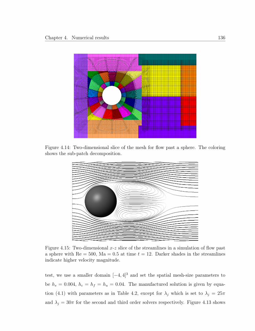
Chapter 4. Numerical results 136
Figure 4.14: Two-dimensional slice of the mesh for flow past a sphere. The coloringshows the sub-patch decomposition.
Figure 4.15: Two-dimensional x-z slice of the streamlines in a simulation of flow pasta sphere with Re = 500, Ma = 0.5 at time t = 12. Darker shades in the streamlinesindicate higher velocity magnitude.
test, we use a smaller domain [−4, 4]3 and set the spatial mesh-size parameters to
be hs = 0.004, hc = hf = hu = 0.04. The manufactured solution is given by equa-
tion (4.1) with parameters as in Table 4.2, except for λj which is set to λj = 25π
and λj = 30π for the second and third order solvers respectively. Figure 4.13 shows
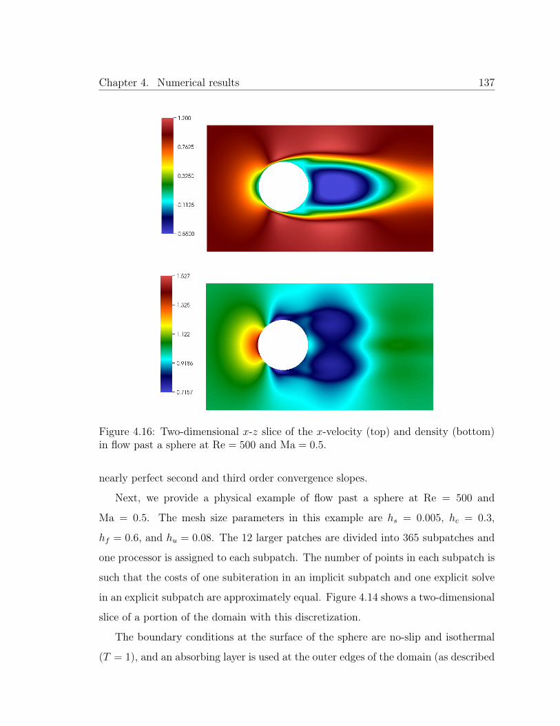
Chapter 4. Numerical results 137
Figure 4.16: Two-dimensional x-z slice of the x-velocity (top) and density (bottom)in flow past a sphere at Re = 500 and Ma = 0.5.
nearly perfect second and third order convergence slopes.
Next, we provide a physical example of flow past a sphere at Re = 500 and
Ma = 0.5. The mesh size parameters in this example are hs = 0.005, hc = 0.3,
hf = 0.6, and hu = 0.08. The 12 larger patches are divided into 365 subpatches and
one processor is assigned to each subpatch. The number of points in each subpatch is
such that the costs of one subiteration in an implicit subpatch and one explicit solve
in an explicit subpatch are approximately equal. Figure 4.14 shows a two-dimensional
slice of a portion of the domain with this discretization.
The boundary conditions at the surface of the sphere are no-slip and isothermal
(T = 1), and an absorbing layer is used at the outer edges of the domain (as described
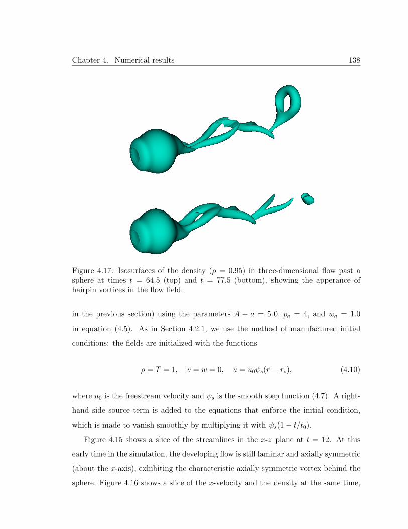
Chapter 4. Numerical results 138
Figure 4.17: Isosurfaces of the density (ρ = 0.95) in three-dimensional flow past asphere at times t = 64.5 (top) and t = 77.5 (bottom), showing the apperance ofhairpin vortices in the flow field.
in the previous section) using the parameters A − a = 5.0, pa = 4, and wa = 1.0
in equation (4.5). As in Section 4.2.1, we use the method of manufactured initial
conditions: the fields are initialized with the functions
ρ = T = 1, v = w = 0, u = u0ψs(r − rs), (4.10)
where u0 is the freestream velocity and ψs is the smooth step function (4.7). A right-
hand side source term is added to the equations that enforce the initial condition,
which is made to vanish smoothly by multiplying it with ψs(1− t/t0).
Figure 4.15 shows a slice of the streamlines in the x-z plane at t = 12. At this
early time in the simulation, the developing flow is still laminar and axially symmetric
(about the x-axis), exhibiting the characteristic axially symmetric vortex behind the
sphere. Figure 4.16 shows a slice of the x-velocity and the density at the same time,

Chapter 4. Numerical results 139
which shows that vortices may be characterized by areas of low density relative to the
freestream density. In Figure 4.17, snapshots of density isosurfaces indicate the shed-
ding of “hairpin” shaped vortices, the character of which are qualitatively consistent
with the results of similar experiments and numerical simulations for incompressible
flow [50,55,56,74].

Chapter 5. Conclusions and future work 140
Chapter 5
Conclusions and future work
This thesis introduced a multi-domain implicit-explicit solution strategy for the com-
pressible Navier-Stokes equations. A solid theoretical foundation, including proofs of
unconditional stability and quasi-unconditional stability for related linear problems
was presented for the implicit component (the BDF-ADI solver) of the proposed multi-
domain implicit-explicit solver. The explicit overset FC strategy was extended to the
implicit-explicit context. The resulting overall capability provides a basic framework
for solvers applicable to significantly more complex geometries, physical problems,
and PDEs. The numerical examples presented in this text demonstrate the meaning-
ful advantages inherent in the proposed solvers, which include higher-order accuracy
in both space and time, dispersionlessness, quasi-unconditional stability for the BDF-
ADI solvers, and efficient parallel implementation. The methodologies introduced in
this thesis thus provide general-geometry solvers that can resolve boundary layers
and other flow features without recourse to crippling time steps, they can evaluate
flow fields with high accuracy, and, in particular, they provide quasi-unconditional
stability in boundary regions with theoretically and numerically demonstrated orders
of temporal accuracy as high as s = 6.
Much remains to be done. The theoretical analyses presented in this thesis
should be extended to problems more closely resembling the compressible Navier-
Stokes equations—including for example variable coefficient equations, higher dimen-

Chapter 5. Conclusions and future work 141
sions, systems of equations, and nonlinearities. Future analyses should also include
a wider array of spatial discretizations of interest, such as finite differences, Cheby-
shev spectral methods, and FC. Importantly, further, it should be useful to study
the possible applicability of the ideas introduced in this thesis to other types of
splitting schemes where intermediate variables arise which require use of potentially
non-physical boundary conditions (e.g., schemes that split velocity and pressure com-
ponents in the incompressible Navier-Stokes equations; see for example the concise
discussion [76, pp. 74-76]).
The software itself should be improved:
1. The multi-domain solver should use a sub-patch decomposition strategy that
assigns processors to implicit and explicit sub-patches in such a way as to min-
imize idle times;
2. A scheduling algorithm should be developed to assign an implicit or explicit
solver to a particular sub-patch on the fly, taking into account global and local
CFL constraints to produce the most efficient computing time with the maxi-
mum possible time step;
3. An accelerated overset subiteration strategy should be developed: since, as
pointed out in Section 3.4.1, the error between subiteration solutions and the
exact solution is localized at the boundary and drops off exponentially from
there, instead of performing a subiteration on the entire domain, it should be
possible to restrict inter-iteration updates to a vicinity of the boundary only—
which would essentially reduce the cost of each subiteration from a d to a d− 1
dimensional problem, resulting in massive savings.
Finally, the software should be exercised to the fullest extent of its capacities,
which in itself amounts to a significantly challenging endeavor.

Appendix A. Matrices for quasilinear-like Navier-Stokes formulation 142
Appendix A
Matrices for quasilinear-likeNavier-Stokes formulation
Let u = (u, v, w)T be the velocity vector in Cartesian coordinates. For simplicity of
presentation, let a =1
Re
µ′(T )
ρ, b =
γ(γ − 1)Ma2
Re
µ(T )
ρ, c =
γ
RePr
κ′(T )
ρ, d =
1
γMa2 ,
and e = γ−1. The coefficient matrices for the Navier-Stokes equations in quasilinear-
like Cartesian form (2.2) are
Mx =
u− 23aTx − 1
2aTy − 1
2aTz d−a(ux− 1
3∇·u) dT
ρ
13aTy u− 1
2aTx 0 − 1
2a(vx+uy) 0
13aTz 0 u− 1
2aTx − 1
2a(wx+uz) 0
eT−b(2ux− 23∇·u) −b(vx+uy) −b(wx+uz) u−cTx 0
ρ 0 0 0 u
,
My =
v− 12aTy
13aTx 0 − 1
2a(vx+uy) 0
− 12aTx v− 2
3aTy − 1
2aTz d−a(vy− 1
3∇·u) dT
ρ
0 13aTz v− 1
2aTy − 1
2a(wy+vz) 0
−b(vx+uy) eT−b(2vy− 23∇·u) −b(wy+vz) v−cTy 0
0 ρ 0 0 v
,
M z =
w− 12aTz 0 1
3aTx − 1
2a(wx+uz) 0
0 w− 12aTz
13aTy − 1
2a(wy+vz) 0
− 12aTx − 1
2aTy w− 2
3aTz d−a(wz− 1
3∇·u) dT
ρ
−b(wx+uz) −b(wy+vz) eT−b(2wz− 23∇·u) w−cTz 0
0 0 ρ 0 w
,

Appendix A. Matrices for quasilinear-like Navier-Stokes formulation 143
Mxx = − 1
Re ρdiag
(4
3µ, µ, µ,
γ
Prκ, 0
),
Myy = − 1
Re ρdiag
(µ,
4
3µ, µ,
γ
Prκ, 0
),
M zz = − 1
Re ρdiag
(µ, µ,
4
3µ,
γ
Prκ, 0
).
The matrices Mxy, Mxz, and Myz are zero except for two elements each, which are
Mxyu,v = Mxy
v,u = Mxzu,w = Mxz
w,u = Myzv,w = Myz
w,v = −1
3
1
Re
µ
ρ.
Using the above definitions and the metric terms ξx, ξy, etc. the coefficient ma-
trices in general coordinates for use in (2.5) as computed by the chain rule are given
by
M ξ,1 =ξxMx + ξyM
y + ξzMz + ξxxM
xx + ξyyMyy + ξzzM
zz
+ ξxyMxy + ξxzM
xz + ξyzMyz,
M ξ,2 = ξ2xM
xx + ξ2yM
yy + ξ2zM
zz + ξxξyMxy + ξxξzM
xz + ξyξzMyz,
and Mη,1, Mη,2 (resp. M ζ,1, M ζ,2) are obtained by replacing ξ with η (resp. ζ) ev-
erywhere in the above two equations. The mixed-derivative matrices can be obtained

Appendix A. Matrices for quasilinear-like Navier-Stokes formulation 144
similarly and are given by
M ξη = ξxηxMxx + ξyηyM
yy + ξzηzMzz
+ (ξxηy + ηxξy)Mxy + (ξxηz + ηxξz)M
xz + (ξyηz + ηyξz)Myz,
M ξζ = ξxζxMxx + ξyζyM
yy + ξzζzMzz
+ (ξxζy + ζxξy)Mxy + (ξxζz + ζxξz)M
xz + (ξyζz + ζyξz)Myz,
Mηζ = ηxζxMxx + ηyζyM
yy + ηzζzMzz
+ (ηxζy + ζxηy)Mxy + (ηxζz + ζxηz)M
xz + (ηyζz + ζyηz)Myz.

Appendix B. Notes on mesh generation 145
Appendix B
Notes on mesh generation
This appendix provides details regarding the algebraic mesh generation of the curvi-
linear patches used in the examples of flow past a cylinder and flow past a sphere
(Sections 4.2.1 and 4.2.2 respectively).
The annular sections pictured in Figure 4.9 were generated by means of the for-
mulae
x(ξ, η) = r(ξ, η) cos θ(ξ), (B.1)
y(ξ, η) = r(ξ, η) sin θ(ξ), (B.2)
r(ξ, η) =(1− η3)rmin + η3rmax + η(1− η2)r′in
1− η + η[cosp θ(ξ) + sinp θ(ξ)]1/p, (B.3)
θ(ξ) = (1− ξ)θmin + ξθmax, (B.4)
with ξ, η ∈ [0, 1] and domain parameters rmin, rmax, r′in, θmin, θmax and p. The
denominator of r produces a “rounded square” outer boundary for p > 2: larger
values of p result in sharper corners (p = 2 produces a circular annular section). The
annular sections in Figure 4.9 use p = 8. The numerator of r controls the radial
extents of the domain as well as ensuring that ∂ηr|η=0 = r′in. The parameter r′in and
number of discretization points in the η direction can then be chosen to produce the
desired radial spacing near the surface of the cylinder and at the outer edge of the
annular sections.

Appendix B. Notes on mesh generation 146
Figure B.1: Left: The “Yin” mesh with coarser grid spacing than used in the numericalexamples of flow past a sphere. Right: The composite “Yin-Yang” mesh.
The curvilinear patches in the example of flow past a sphere are based on the
so-called “Yin-Yang” mesh [51], which provides a (volumetric) covering of the sphere
with two logically rectangular patches. As in the annular mesh above, the original
formulae are modified to produce a “rounded cube” appearance and allow for variable
radial mesh spacing. In detail, the formula for the Yin mesh is given by
x(ξ, η, ζ) = r(ξ, η, ζ) cos θ(ξ) sinφ(η), (B.5)
y(ξ, η, ζ) = r(ξ, η, ζ) sin θ(ξ) sinφ(η), (B.6)
z(ξ, η, ζ) = r(ξ, η, ζ) cosφ(η), (B.7)
r(ξ, η, ζ) =(rmax − rmin)f(ζ)
rmax − f(ζ) + (f(ζ)− rmin)g(ξ, η), (B.8)
g(ξ, η) = [(cosp θ(ξ) + sinp θ(ξ)) sinp φ(η) + cosp φ(η)]1/p , (B.9)
f(ζ) = (1− ζ2)rmin + ζ2rmax + ζ(1− ζ)r′in, (B.10)
θ(ξ) = (1− ξ)θmin + ξθmax, (B.11)
φ(η) = (1− η)φmin + ηφmax, (B.12)
with ξ, η ∈ [0, 1] and domain parameters rmin, rmax, r′in, θmin, θmax, φmin, φmax, and p

Appendix B. Notes on mesh generation 147
(which is set to p = 8). Again, r′in and the number of ζ discretization points are chosen
to produce the desired radial grid spacing at the surface of the sphere and at the outer
edge of the mesh. The resulting mesh is shown in the left pane of Figure B.1, with
much coarser grid spacing than used in the numerical examples (for clarity). The x,
y, and z equations for the Yang mesh are given by
x(ξ, η, ζ) = r(ξ, η, ζ) cosφ(η), (B.13)
y(ξ, η, ζ) = r(ξ, η, ζ) sin θ(ξ) sinφ(η), (B.14)
z(ξ, η, ζ) = r(ξ, η, ζ) cos θ(ξ) sinφ(η). (B.15)
The remaining equations are the same as for the Yin mesh. The right pane of Fig-
ure B.1 shows the composite overlapping mesh.
Bibliography 148
Bibliography
[1] Abarbanel, S., Gottlieb, D., and Carpenter, M. H. On the removal of
boundary errors caused by Runge-Kutta integration of nonlinear partial differ-
ential equations. SIAM Journal on Scientific Computing 17, 3 (1996), 777–782.
[2] Albin, N., and Bruno, O. P. A spectral FC solver for the compressible
Navier–Stokes equations in general domains I: Explicit time-stepping. Journal
of Computational Physics 230, 16 (July 2011), 6248–6270.
[3] Amlani, F. A new high-order Fourier continuation-based elasticity solver for
complex three-dimensional geometries. PhD, California Institute of Technology,
2014.
[4] Ascher, U. M., Ruuth, S. J., and Wetton, B. T. Implicit-explicit methods
for time-dependent partial differential equations. SIAM Journal on Numerical
Analysis 32, 3 (1995), 797–823.
[5] Ashcroft, G., and Zhang, X. Optimized prefactored compact schemes.
Journal of Computational Physics 190, 2 (2003), 459–477.
[6] Beam, R. M., and Warming, R. An implicit factored scheme for the com-
pressible Navier-Stokes equations. AIAA journal 16, 4 (1978), 393–402.
[7] Beam, R. M., and Warming, R. Alternating direction implicit methods for
parabolic equations with a mixed derivative. SIAM Journal on Scientific and
Statistical Computing 1, 1 (1980), 131–159.

Bibliography 149
[8] Beam, R. M., and Warming, R. F. An implicit finite-difference algorithm for
hyperbolic systems in conservation-law form. Journal of Computational Physics
22, 1 (Sept. 1976), 87–110.
[9] Bijl, H., Carpenter, M. H., Vatsa, V. N., and Kennedy, C. A. Implicit
time integration schemes for the unsteady compressible Navier–Stokes equations:
laminar flow. Journal of Computational Physics 179, 1 (June 2002), 313–329.
[10] Boyd, J. P. Chebyshev and Fourier spectral methods. Courier Dover Publica-
tions, 2001.
[11] Briley, W. R., and McDonald, H. Solution of the three-dimensional com-
pressible Navier-Stokes equations by an implicit technique. In Proceedings of
the Fourth International Conference on Numerical Methods in Fluid Dynamics
(1975), Springer, pp. 105–110.
[12] Briley, W. R., and McDonald, H. On the structure and use of linearized
block implicit schemes. Journal of Computational Physics 34, 1 (Jan. 1980),
54–73.
[13] Brown, D. L., Henshaw, W. D., and Quinlan, D. J. Overture: Object-
oriented tools for overset grid applications. AIAA paper No. 99 9130 (1999).
[14] Bruno, O. P., Han, Y., and Pohlman, M. M. Accurate, high-order represen-
tation of complex three-dimensional surfaces via Fourier continuation analysis.
Journal of Computational Physics 227, 2 (2007), 1094–1125.
[15] Bruno, O. P., and Jimenez, E. Higher-order linear-time unconditionally
stable alternating direction implicit methods for nonlinear convection-diffusion
partial differential equation systems. Journal of Fluids Engineering 136, 6 (Apr.
2014), 060904–060904.
Bibliography 150
[16] Bruno, O. P., and Lyon, M. High-order unconditionally stable FC-AD solvers
for general smooth domains I. Basic elements. Journal of Computational Physics
229, 6 (Mar. 2010), 2009–2033.
[17] Bruno, O. P., and Prieto, A. Spatially dispersionless, unconditionally stable
FC–AD solvers for variable-coefficient PDEs. Journal of Scientific Computing
58, 2 (2014), 331–366.
[18] Canuto, C., Hussaini, M. Y., Quarteroni, A., and Zang, T. A. Spectral
methods: evolution to complex geometries and applications to fluid dynamics.
Springer Science & Business Media, June 2007.
[19] Canuto, C., Hussaini, M. Y., Quarteroni, A., and Zang, T. A. Spectral
methods: fundamentals in single domains. Springer Science & Business Media,
Sept. 2007.
[20] Carpenter, M. H., Gottlieb, D., Abarbanel, S., and Don, W.-S. The
theoretical accuracy of Runge-Kutta time discretizations for the initial boundary
value problem: a study of the boundary error. SIAM Journal on Scientific
Computing 16, 6 (1995), 1241–1252.
[21] Chesshire, G., and Henshaw, W. D. Composite overlapping meshes for the
solution of partial differential equations. Journal of Computational Physics 90,
1 (1990), 1–64.
[22] Chorin, A. J. Numerical solution of the Navier-Stokes equations. Mathematics
of Computation 22, 104 (1968), 745–762.
[23] Courant, R., Friedrichs, K., and Lewy, H. Über die partiellen Dif-
ferenzengleichungen der mathematischen Physik. Mathematische Annalen 100,
1 (1928), 32–74.

Bibliography 151
[24] Crank, J., and Nicolson, P. A practical method for numerical evaluation
of solutions of partial differential equations of the heat-conduction type. Math-
ematical Proceedings of the Cambridge Philosophical Society 43, 01 (Jan. 1947),
50–67.
[25] Curtiss, C. F., and Hirschfelder, J. Integration of stiff equations. Pro-
ceedings of the National Academy of Sciences of the United States of America
38, 3 (1952), 235.
[26] Dahlquist, G. Convergence and stability in the numerical integration of ordi-
nary differential equations. Math. Scand 4, 1 (1956), 33–53.
[27] Dahlquist, G. 33 years of numerical instability, Part I. BIT Numerical Math-
ematics 25, 1 (Mar. 1985), 188–204.
[28] Dahlquist, G. G. A special stability problem for linear multistep methods.
BIT Numerical Mathematics 3, 1 (Mar. 1963), 27–43.
[29] Daniel, J. W., and Moore, R. E. Computation and theory in ordinary
differential equations. Freeman, Dec. 1970.
[30] Douglas, Jr., J. On the Numerical Integration of u_xx + u_yy = u_t by
Implicit Methods. Journal of the Society for Industrial and Applied Mathematics
3, 1 (Mar. 1955), 42–65.
[31] Douglas, Jr., J., and Gunn, J. E. Alternating direction methods for
parabolic systems in M space variables. J. ACM 9, 4 (Oct. 1962), 450–456.
[32] Douglas Jr., J., and Gunn, J. E. A general formulation of alternating
direction methods. Numerische Mathematik 6, 1 (Dec. 1964), 428–453.
[33] D’yakonov, E. G. Difference schemes with splitting operator for higherdimen-
sional non-stationary problems. USSR. Comput. Math. Math. Phys 2, 4 (1962),
549–568.

Bibliography 152
[34] Ekaterinaris, J. A. Implicit, high-resolution, compact schemes for gas dy-
namics and aeroacoustics. Journal of Computational Physics 156, 2 (Dec. 1999),
272–299.
[35] Elling, T. J. GPU-accelerated Fourier-continuation solvers and physically ex-
act computational boundary conditions for wave scattering problems. PhD, Cal-
ifornia Institute of Technology, 2013.
[36] Fairweather, G., and Mitchell, A. R. A new computational procedure
for A.D.I. methods. SIAM Journal on Numerical Analysis 4, 2 (June 1967),
163–170.
[37] Forti, D., and Dedè, L. Semi–implicit BDF time discretization of the
Navier–Stokes equations with VMS–LES modeling in a high performance com-
puting framework. Computers & Fluids (2015).
[38] Gaitonde, D. V., and Visbal, M. R. High-order schemes for Navier-Stokes
equations: algorithm and implementation into FDL3di. Tech. rep., DTIC Doc-
ument, 1998.
[39] Gaitonde, D. V., and Visbal, M. R. Pade-type higher-order boundary filters
for the Navier-Stokes equations. AIAA Journal 38, 11 (2000), 2103–2112.
[40] Gander, M. J., and others. Schwarz methods over the course of time.
Electronic Transactions on Numerical Analysis 31, 228-255 (2008), 5.
[41] Gordnier, R. E. High fidelity computational simulation of a membrane wing
airfoil. Journal of Fluids and Structures 25, 5 (July 2009), 897–917.
[42] Gordon, W. J., and Hall, C. A. Construction of curvilinear co-ordinate sys-
tems and applications to mesh generation. International Journal for Numerical
Methods in Engineering 7, 4 (1973), 461–477.
Bibliography 153
[43] Gottlieb, D., and Hesthaven, J. S. Spectral methods for hyperbolic prob-
lems. Journal of Computational and Applied Mathematics 128, 1 (2001), 83–131.
[44] Gottlieb, D., and Shu, C.-W. On the Gibbs phenomenon and its resolution.
SIAM Review 39, 4 (1997), 644–668.
[45] Gustafsson, B., Kreiss, H., and Oliger, J. Time-dependent problems and
difference methods. Pure and Applied Mathematics: A Wiley Series of Texts,
Monographs and Tracts. Wiley, 2013.
[46] Hairer, E., and Wanner, G. Solving ordinary differential equations II. Stiff
and differential-algebraic problems. Springer Series in Computational Mathemat-
ics, 2005.
[47] Hesthaven, J. S., Gottlieb, S., and Gottlieb, D. Spectral methods for
time-dependent problems, vol. 21. Cambridge University Press, 2007.
[48] Hoffmann, K. A., and Chiang, S. T. Computational fluid dynamics, vol. 2.
Engineering Education System, Wichita, Kansas (2000), 21–46.
[49] Howarth, L. Concerning the effect of compressibility on laminar boundary
layers and their separation. Proceedings of the Royal Society of London. Series
A. Mathematical and Physical Sciences 194, 1036 (July 1948), 16–42.
[50] Johnson, T. A., and Patel, V. C. Flow past a sphere up to a Reynolds
number of 300. Journal of Fluid Mechanics 378 (Jan. 1999), 19–70.
[51] Kageyama, A., and Sato, T. “Yin-Yang grid”: An overset grid in spherical
geometry. Geochemistry, Geophysics, Geosystems 5, 9 (Sept. 2004), Q09005.
[52] Kao, K.-H., and Chow, C.-Y. Linear stability of compressible Taylor–Couette
flow. Physics of Fluids A: Fluid Dynamics (1989-1993) 4, 5 (May 1992), 984–996.

Bibliography 154
[53] Karaa, S. A hybrid Padé ADI scheme of higher-order for convection–diffusion
problems. International Journal for Numerical Methods in Fluids 64, 5 (2010),
532–548.
[54] Kawai, S., and Lele, S. K. Large-eddy simulation of jet mixing in supersonic
crossflows. AIAA Journal 48, 9 (2010), 2063–2083.
[55] Kim, D., and Choi, H. Laminar flow past a sphere rotating in the streamwise
direction. Journal of Fluid Mechanics 461 (June 2002), 365–386.
[56] Kiya, M., Ishikawa, H., and Sakamoto, H. Near-wake instabilities and
vortex structures of three-dimensional bluff bodies: a review. Journal of Wind
Engineering and Industrial Aerodynamics 89, 14 (2001), 1219–1232.
[57] Kopriva, D. A. Implementing spectral methods for partial differential equations:
Algorithms for scientists and engineers. Springer Science & Business Media,
2009.
[58] Lambert, J. D. Numerical methods for ordinary differential systems: the initial
value problem. John Wiley & Sons, Inc., 1991.
[59] Lax, P. D., and Richtmyer, R. D. Survey of the stability of linear finite
difference equations. Communications on Pure and Applied Mathematics 9, 2
(1956), 267–293.
[60] Lele, S. K. Compact finite difference schemes with spectral-like resolution.
Journal of Computational Physics 103, 1 (1992), 16–42.
[61] LeVeque, R. Finite difference methods for ordinary and partial differential
equations. Society for Industrial and Applied Mathematics, Jan. 2007.
[62] Leveque, R. J. Intermediate boundary conditions for LOD, ADI and approxi-
mate factorization methods. Technical Report NASA-CR-172591, ICASE-85-21,
NASA, Mar. 1985.

Bibliography 155
[63] Lions, P.-L. On the Schwarz alternating method. I. In First International
Symposium on Domain Decomposition Methods for Partial Differential Equations
(1988), Paris, France, pp. 1–42.
[64] Lyon, M., and Bruno, O. P. High-order unconditionally stable FC-AD solvers
for general smooth domains II. Elliptic, parabolic and hyperbolic PDEs; theo-
retical considerations. Journal of Computational Physics 229, 9 (May 2010),
3358–3381.
[65] Manela, A., and Frankel, I. On the compressible Taylor–Couette problem.
Journal of Fluid Mechanics 588 (2007), 59–74.
[66] Marques, F., and Lopez, J. M. Onset of three-dimensional unsteady states in
small-aspect-ratio Taylor–Couette flow. Journal of Fluid Mechanics 561 (2006),
255–277.
[67] Mattsson, K., Svärd, M., and Shoeybi, M. Stable and accurate schemes
for the compressible Navier–Stokes equations. Journal of Computational Physics
227, 4 (Feb. 2008), 2293–2316.
[68] Nordström, J., Gong, J., Van der Weide, E., and Svärd, M. A
stable and conservative high order multi-block method for the compressible
Navier–Stokes equations. Journal of Computational Physics 228, 24 (2009),
9020–9035.
[69] Peaceman, D. W., and Rachford, Jr., H. H. The numerical solution of
parabolic and elliptic differential equations. Journal of the Society for Industrial
and Applied Mathematics 3, 1 (Mar. 1955), 28–41.
[70] Pearson, C. E. A computational method for viscous flow problems. Journal
of Fluid Mechanics 21, 04 (Apr. 1965), 611–622.

Bibliography 156
[71] Pfister, G., Schmidt, H., Cliffe, K. A., and Mullin, T. Bifurcation
phenomena in Taylor-Couette flow in a very short annulus. Journal of Fluid
Mechanics 191 (1988), 1–18.
[72] Rizzetta, D. P., Visbal, M. R., and Morgan, P. E. A high-order compact
finite-difference scheme for large-eddy simulation of active flow control. Progress
in Aerospace Sciences 44, 6 (Aug. 2008), 397–426.
[73] Saad, Y., and Schultz, M. H. GMRES: A generalized minimal residual
algorithm for solving nonsymmetric linear systems. SIAM Journal on Scientific
and Statistical Computing 7, 3 (1986), 856–869.
[74] Sakamoto, H., and Haniu, H. A study on vortex shedding from spheres in
a uniform flow. Journal of Fluids Engineering 112, 4 (1990), 386–392.
[75] Schwarz, H. A. Ueber einige Abbildungsaufgaben. Journal für die reine und
angewandte Mathematik 70 (1869), 105–120.
[76] Segal, I. A. Finite element methods for the incompressible Navier-Stokes equa-
tions. Delft University of Technology (2015).
[77] Shih, T. I., Smith, G. E., Springer, G. S., and Rimon, Y. Boundary
conditions for the solution of compressible Navier-Stokes equations by an implicit
factored method. Journal of Computational Physics 52, 1 (1983), 54–79.
[78] Sone, Y. Kinetic theory and fluid dynamics. Modeling and Simulation in Sci-
ence, Engineering and Technology. Birkhäuser Boston, 2012.
[79] Starius, G. Composite mesh difference methods for elliptic boundary value
problems. Numerische Mathematik 28, 2 (June 1977), 243–258.
[80] Steger, J. L., Dougherty, F. C., and Benek, J. A. A chimera grid scheme.
Advances in Grid Generation (June 1983).
Bibliography 157
[81] Strikwerda, J. C. Finite difference schemes and partial differential equations.
SIAM, 2004.
[82] Svärd, M., Carpenter, M. H., and Nordström, J. A stable high-order
finite difference scheme for the compressible Navier–Stokes equations, far-field
boundary conditions. Journal of Computational Physics 225, 1 (2007), 1020–
1038.
[83] Svärd, M., and Nordström, J. A stable high-order finite difference scheme
for the compressible Navier–Stokes equations: No-slip wall boundary conditions.
Journal of Computational Physics 227, 10 (May 2008), 4805–4824.
[84] Tam, C. K. W., and Kurbatskii, K. A. Multi-size-mesh multi-time-step
dispersion-relation-preserving scheme for multiple-scales aeroacoustics problems.
International Journal of Computational Fluid Dynamics 17, 2 (2003), 119–132.
[85] Tam, C. K. W., and Webb, J. C. Dispersion-relation-preserving finite dif-
ference schemes for computational acoustics. Journal of Computational Physics
107, 2 (Aug. 1993), 262–281.
[86] Thomas, P. D., and Neier, K. L. Navier-Stokes simulation of three-
dimensional hypersonic equilibrium flows with ablation. Journal of Spacecraft
and Rockets 27, 2 (1990), 143–149.
[87] Trefethen, L. N. Pseudospectra of linear operators. SIAM review 39, 3 (1997),
383–406.
[88] Trefethen, L. N., and Embree, M. Spectra and pseudospectra: the behavior
of nonnormal matrices and operators. Princeton University Press, 2005.
[89] Uzun, A., and Hussaini, M. Y. Simulation of noise generation in the near-
nozzle region of a chevron nozzle jet. AIAA Journal 47, 8 (2009), 1793–1810.

Bibliography 158
[90] Visbal, M. R., and Gaitonde, D. V. High-order-accurate methods for com-
plex unsteady subsonic flows. AIAA Journal 37, 10 (1999), 1231–1239.
[91] Visbal, M. R., and Gaitonde, D. V. On the use of higher-order finite-
difference schemes on curvilinear and deforming meshes. Journal of Computa-
tional Physics 181, 1 (Sept. 2002), 155–185.
[92] Volkov, E. A. The method of composite meshes for finite and infinite regions
with piecewise smooth boundary. Trudy Matematicheskogo Instituta im. VA
Steklova 96 (1968), 117–148.
[93] Wanner, G., Hairer, E., and Nørsett, S. P. Order stars and stability
theorems. BIT Numerical Mathematics 18, 4 (Dec. 1978), 475–489.
[94] Warming, R. F., and Beam, R. M. An extension of A-stability to alternating
direction implicit methods. BIT Numerical Mathematics 19, 3 (Sept. 1979), 395–
417.
[95] White, F. M., and Corfield, I. Viscous fluid flow, vol. 3. McGraw-Hill New
York, 2006.
[96] Yanenko, N. N. The method of fractional steps. Springer, 1971.
Copyright © 2022 FDOKUMEN