9

Parallelizing PDE Solvers Using the PythonProgramming Language

Xing Cai and Hans Petter Langtangen

Simula Research Laboratory, P.O. Box 134, NO-1325 Lysaker, Norway

Department of Informatics, University of Oslo, P.O. Box 1080, Blindern,NO-0316 Oslo, Norway

[xingca,hpl]@simula.no

Summary. This chapter aims to answer the following question: Can the high-level program-ming language Python be used to develop sufficiently efficient parallel solvers for partialdifferential equations (PDEs)? We divide our investigation into two aspects, namely (1) theachievable performance of a parallel program that extensively uses Python programming andits associated data structures, and (2) the Python implementation of generic software mod-ules for parallelizing existing serial PDE solvers. First of all, numerical computations needto be based on the special array data structure of the Numerical Python package, either inpure Python or in mixed-language Python-C/C++ or Python/Fortran setting. To enable high-performance message passing in parallel Python software, we use the small add-on packagepypar, which provides efficient Python wrappers to a subset of MPI routines. Using con-crete numerical examples of solving wave-type equations, we will show that a mixed Python-C/Fortran implementation is able to provide fully comparable computational speed in com-parison with a pure C or Fortran implementation. In particular, a serial legacy Fortran 77 codehas been parallelized in a relatively straightforward manner and the resulting parallel Pythonprogram has a clean and simple structure.

9.1 Introduction

Solving partial differential equations (PDEs) on a computer requires writing soft-ware to implement numerical schemes, and the resulting program should be ableto effectively utilize the modern computer architecture. The computing power ofparallel platforms is particularly difficult to exploit, so we would like to avoid im-plementing every thing from scratch when developing a parallel PDE solver. Thewell-tested computational modules within an existing serial PDE solver should insome way participate in the parallel computations. Most of the parallelization effortshould be invested in dealing with the parallel-specific tasks, such as domain parti-tioning, load balancing, high performance communication etc. Such considerationscall for a flexible, structured, and layered programming style for developing parallelPDE software. The object-oriented programming language C++, in particular, hasobtained a considerable amount of success in this field, see e.g. [2, 3, 15, 4, 13].

296 X. Cai and H. P. Langtangen

In comparison with C++, the modern object-oriented programming languagePython is known for its even richer expressiveness and flexibility. Moreover, thePython language simplifies interfacing legacy software written in the traditional com-piled programming languages Fortran, C, and C++. This is a desired feature in paral-lelizing PDE solvers, because the serial computational modules of a PDE solver andexisting software libraries may exist in different programming styles and languages.However, due to the computational inefficiency of its core language, Python has sel-dom been used for large-scale scientific computations, let alone parallelizations.

Based on the findings in [5], we have reasons to believe that Python is capable ofdelivering high performance in both serial and parallel computations. This assumesthat the involved data structure uses arrays of the Numerical Python package [17].Moreover, either the technique of vectorization must be adopted, or computation-intensive code segments must be migrated to extension modules implemented in acompiled language such as Fortran, C or C++. It is the purpose of the present chapterto show that the clean syntax and the powerful tools of Python help to simplify theimplementation tasks of parallel PDE solvers. We will also show that existing seriallegacy codes and software libraries can be re-used in parallel computations driven byPython programs.

The remainder of the chapter is organized as follows. Section 9.2 presents themost important ingredients in achieving high-performance computing in Python.Section 9.3 explains two parallelization approaches of relevance for PDE solvers,whereas Sections 9.4 gives examples of how Python can be used to code genericfunctions useful for parallelizing serial PDE solvers. Afterwards, Section 9.5 demon-strates two concrete cases of parallelization, and Section 9.6 summarizes the mainissues of this chapter.

9.2 High-Performance Serial Computing in Python

To achieve good performance of any parallel PDE solver, the involved serial com-putational modules must have high performance. This is no exception in the contextof the Python programming language. The present section therefore discusses theissue of high-performance serial computing in Python. Some familiarity with basicPython is assumed. We refer to [14] for an introduction to Python with applicationsto computational science.

9.2.1 Array-Based Computations

PDE solvers frequently employ one-dimensional or multi-dimensional arrays. Com-putations are normally done in the form of nested loops over values stored in thearrays. Such nested loops run very slowly if they are coded in the core language ofPython. However, the add-on package Numerical Python [17], often referred to asNumPy, provides efficient operations on multi-dimensional arrays.

The NumPy package has a basic module defining a data structure of multi-dimensional contiguous-memory arrays and many associated efficient C functions.

9 Parallel PDE Solvers in Python 297

Two versions of this module exist at present: Numeric is the classical module fromthe mid 1990s, while numarray is a new implementation. The latter is meant asa replacement of the former, and no further development of Numeric is going totake place. However, there is so much numerical Python code utilizing Numeric thatwe expect both modules to co-exist for a long time. We will emphasize the use ofNumeric in this chapter, because many tools for scientific Python computing are atpresent best compatible with Numeric.

The allocation and use of NumPy arrays is very user friendly, which can bedemonstrated by the following code segment:

from Numeric import arange, zeros, Floatn = 1000001dx = 1.0/(n-1)x = arange(0, 1, dx) # x = 0, dx, 2*dx, ...y = zeros(len(x), Float) # array of zeros, as long as x

# as Float (=double in C) entriesfrom math import sin, cos # import scalar math functionsfor i in xrange(len(x)): # i=0, 1, 2, ..., length of x-1

xi = x[i]y[i] = sin(xi)*cos(xi) + xi**2

Here the arange method allocates a NumPy array and fills it with values from astart value to (but not including) a stop value using a specified increment. Note that aPython method is equivalent to a Fortran subroutine or a C/C++ function. Allocatinga double precision real-value array of length n is done by the zeros(n,Float) call.Traversing an array can be done by a for-loop as shown, where xrange is a methodthat returns indices 0, 1, 2, and up to (but not including) the length of x (i.e., len(x))in this example. Indices in NumPy arrays always start at 0.

Detailed measurements of the above for-loop show that the Python code is con-siderably slower than a corresponding code implemented in plain Fortran or C. Thisis due to the slow execution of for-loops in Python, even though the NumPy data ar-rays have an efficient underlying C implementation. Unlike the traditional compiledlanguages, Python programs are complied to byte code (like Java). Loops in Pythonare not highly optimized in machine code as Fortran, C, or C++ compilers would do.Such optimizations are in fact impossible due to the dynamic nature of the Pythonlanguage. For example, there is no guarantee that sin(xi) does not return a newdata type at some stage in the loop and thereby turning y into a new data type. (Theonly requirement of the new type is that it must be valid to subscript it as y[i].)In the administering parts of a PDE code, this type of flexibility can be the reasonto adopt Python, but in number crunching with large arrays the efficiency frequentlybecomes unacceptable.

The problem with slow Python loops can be greatly relieved through vectoriza-tion [16], i.e., expressing the loop semantics via a set of basic NumPy array op-erations, where each operation involves a loop over array entries efficiently imple-mented in C. As an improvement of the above Python for-loop, we now introduce avectorized implementation as follows:

from Numeric import arange, sin, cosn = 1000001

298 X. Cai and H. P. Langtangen

dx = 1.0/(n-1)x = arange(0, 1, dx) # x = 0, dx, 2*dx, ...y = sin(x)*cos(x) + x**2

The expression sin(x) applies the sine function to each entry in the array x, thesame for cos(x) and x**2. The loop over the array entries now runs in highlyoptimized C code, and the reference to a new array holding the computed result isreturned. Consequently, there is no need to allocate y beforehand, because an array iscreated by the vector expression sin(x)*cos(x) + x**2. This vectorized versionruns about 8 times faster than the pure Python version. For more information onusing NumPy arrays and vectorization, we refer to [14, 5].

9.2.2 Interfacing with Fortran and C

Vectorized Python code may still run a factor of 3-10 slower than optimized im-plementations in pure Fortran or C/C++. This is not surprising because an expres-sion like sin(x)*cos(x)+x**2 involves three unary operations (sin(x), cos(x),x**2) and two binary operations (multiplication and addition), each begin processedin a separate C routine. For each intermediate result, a temporary array must be allo-cated. This is the same type of overhead involved in compound vector operations inmany other libraries (Matlab/Octave, R/S-Plus, C++ libraries [20, 19]).

In these cases, or in cases where vectorization of an algorithm is cumbersome,computation-intensive Python loops can be easily migrated directly to Fortran orC/C++. The code migration can be easily achieved in Python, using specially de-signed tools such as F2PY [9]. For example, we may implement the expression in asimple loop in Fortran 77:

subroutine someloop(x, n)integer n, ireal*8 x(n), xi

Cf2py intent(in,out) xdo i = 1, n

xi = x(i)x(i) = sin(xi)*cos(xi) + xi**2

end doreturnend

The only non-standard feature of the above Fortran subroutine is the command linestarting with Cf2py. This helps the Python-Fortran translation tool F2PY [9] withinformation about input and output arguments. Note that x is specified as both aninput and an output argument. An existing pure Fortran subroutine can be very easilytransformed by F2PY to be invokable inside a Python program. In particular, theabove someloop method can be called inside a Python program as

y = someloop(x)# orsomeloop(x) # rely on in-place modifications of x

9 Parallel PDE Solvers in Python 299

The “Python” way of writing methods is to have input variables as arguments andreturn all output variables. In the case of someloop(x), the Fortran code overwritesthe input array with values of the output array. The length of the x array is needed inthe Fortran code, but not in the Python call because the length is available from theNumPy array x.

The variable x is a NumPy array object in Python, while the Fortran code expectsa pointer to a contiguous data segment and the array size. The translation of Pythondata to and from Fortran data must be done in wrapper code. The tool F2PY canread Fortran source code files and automatically generate the wrapper code. It is thewrapper code that extracts the array size and the pointer to the array data segmentfrom the NumPy array object and sends these to the Fortran subroutine. The wrappercode also converts the Fortran output data to Python objects. In the present examplewe may store the someloop subroutine in a file named floop.f and run F2PY like

f2py -m floop -c floop.f

This command creates an extension module floop with the wrapper code and thesomeloop routine. The extension module can be imported as any pure Python pro-gram.

Migrating intensive computations to C or C++ via wrapper code can be donesimilarly as explained for Fortran. However, the syntax has a more rigid style andadditional manual programming is needed. There are tools for automatic generationof the wrapper code for C and C++, SWIG [8] for instance, but none of the toolsintegrate C/C++ seamlessly with NumPy arrays as for Fortran. Information on com-puting with NumPy arrays in C/C++ can be found in [1, 14].

9.3 Parallelizing Serial PDE Solvers

Parallel computing is an important technique for solving large-scale PDE problems,where multiple processes form a collaboration to solve a large computational prob-lem. The total computational work is divided into multiple smaller tasks that canbe carried out concurrently by the different processes. In most cases, the collabora-tion between the processes is realized as exchanging computing results and enforc-ing synchronizations. This section will first describe a subdomain-based frameworkwhich is particularly well-suited for parallelizing PDE solvers. Then, two approachesto parallelizing different types of numerical schemes will be explained, in the contextof Python data structures.

9.3.1 A Subdomain-Based Parallelization Framework

The starting point of parallelizing a PDE solver is a division of the global computa-tional work among the processes. The division can be done in several different ways.Since PDE solvers normally involve a lot of loop-based computations, one strategyis to (dynamically) distribute the work of every long loop among the processes. Sucha strategy often requires that all the processes have equal access to all the data, and

300 X. Cai and H. P. Langtangen

that a master-type process is responsible for (dynamically) carrying out the workload distribution. Therefore, shared memory is the most suitable platform type forthis strategy. In this chapter, however, we will consider dividing the work based onsubdomains. That is, a global solution domain Ω is explicitly decomposed into aset of subdomains ∪Ωs = Ω, where there may be an overlap zone between eachpair of neighboring subdomains. The part of the subdomain boundary that borders aneighboring subdomain, i.e., ∂Ωs\∂Ω, is called the internal boundary of Ωs. Thisdecomposition of the global domain gives rise to a decomposition of the global dataarrays, where subdomain s always concentrates on the portion of the global dataarrays lying inside Ωs. Such a domain and data decomposition results in a naturaldivision of the global computational work among the processes, where the compu-tational work on one subdomain is assigned to one process. This strategy suits bothshared-memory and distributed-memory platforms.

In addition to ensuring good data locality on each process, the subdomain-basedparallelization strategy also strongly promotes code re-use. One scenario is that partsof an existing serial PDE solver are used to carry out array-level operations (seeSection 9.3.2), whereas another scenario is that an entire serial PDE solver worksas a “black box subdomain solver” in Schwarz-type iterations (see Section 9.3.3).Of course, communication between subdomains must be enforced at appropriate lo-cations of a parallel PDE solver. It will be shown in the remainder of this sectionthat the needed communication operations are of a generic type, independent of thespecific PDE problem. Moreover, Section 9.4 will show that Python is a well-suitedprogramming language for implementing the generic communication operations asre-usable methods.

9.3.2 Array-Level Parallelization

Many numerical operations can be parallelized in a straightforward manner, whereexamples are (1) explicit time-stepping schemes for time-dependent PDEs, (2) Ja-cobi iterations for solving a system of linear equations, (3) inner-products betweentwo vectors, and (4) matrix-vector products. The parallel version of these operationscomputes identical numerical results as the serial version. Therefore, PDE solversinvolving only such numerical operations are readily parallelizable. Inside the frame-work of subdomains, the basic idea of this parallelization approach is as follows:

1. The mesh points of each subdomain are categorized into two groups: (1) pointslying on the internal boundary and (2) the interior points (plus points lying on thephysical boundary). Each subdomain is only responsible for computing valueson its interior points (plus points lying on the physical boundary). The valueson the internal boundary points are computed by the neighboring subdomainsand updated via communication. (Such internal boundary points are commonlycalled ghost points.)

2. The global solution domain is partitioned such that there is an overlap zone ofminimum size between two neighboring subdomains. For a standard second-order finite difference method this means one layer of overlapping cells (higher

9 Parallel PDE Solvers in Python 301

order finite differences require more overlapping layers), while for finite elementmethods this means one layer of overlapping elements. Such an overlappingdomain partitioning ensures that every internal boundary point of one subdomainis also located in the interior of at least one neighboring subdomain.

3. The parallelization of a numerical operation happens at the array level. That is,the numerical operation is concurrently carried out on each subdomain using itslocal arrays. When new values on the interior points are computed, neighboringsubdomains communicate with each other to update the values on their internalboundary points.

Now let us consider a concrete example of parallelizing the following five-pointstencil operation (representing a discrete Laplace operator) on a two-dimensionalarray um, where the computed results are stored in another array u:

for i in xrange(1,nx):for j in xrange(1,ny):

u[i,j] = um[i,j-1] + um[i-1,j] \-4*um[i,j] + um[i+1,j] + um[i,j+1]

The above Python code segment is assumed to be associated with a uniform two-dimensional mesh, having nx cells (i.e., nx + 1 entries) in the x-direction and ny

cells (i.e., ny + 1 entries) in the y-direction. Note that the boundary entries of the uarray are assumed to be computed separately using some given boundary condition(not shown in the code segment). We also remark that xrange(1,nx) covers indices1, 2, and up to nx-1 (i.e., not including index nx).

Suppose P processors participate in the parallelization. Let us assume that theP processors form an Nx × Ny = P lattice. A division of the global computationalwork naturally arises if we partition the interior array entries of u and um into P smallrectangular portions, using imaginary horizontal and vertical cutting lines. That is,the (nx − 1) × (ny − 1) interior entries of u and um are divided into Nx × Ny

rectangular portions. For a processor that is identified by an index tuple (l, m), where0 ≤ l < Nx and 0 ≤ m < Ny , (nl

x − 1) × (nmy − 1) interior entries are assigned

to it, plus one layer of boundary entries around the interior entries (i.e., one layer ofoverlapping cells). More precisely, we have

Nx−1∑l=0

(nlx − 1) = nx − 1,

Ny−1∑m=0

(nmy − 1) = ny − 1,

where we require that the values of n0x, n1

x, . . ., and nNx−1x are approximately the

same as(nx − 1)/Nx + 1

for the purpose of achieving a good work load balance. The same requirement shouldalso apply to the values of n0

y , n1y , . . ., and n

Ny−1y .

To achieve a parallel execution of the global five-point stencil operation, eachprocessor now loops over its (nl

x−1)×(nmy −1) interior entries of u loc as follows:

302 X. Cai and H. P. Langtangen

for i in xrange(1,loc_nx):for j in xrange(1,loc_ny):

u_loc[i,j] = um_loc[i,j-1] + um_loc[i-1,j] \-4*um_loc[i,j] \+ um_loc[i+1,j] + um_loc[i,j+1]

We note that the physical boundary entries of u loc are assumed to be com-puted separately using some given boundary condition (not shown in the above codesegment). For the internal boundary entries of u loc, communication needs to becarried out. Suppose a subdomain has a neighbor on each of its four sides. Then thefollowing values should be sent out to the neighbors:

• u[1,:] to the negative-x side neighbor,• u[nx loc-1,:] to the positive-x side neighbor,• u[:,1] to the negative-y side neighbor, and• u[:,ny loc-1] to the positive-y side neighbor.

Correspondingly, the following values should be received from the neighbors:

• u[0,:] from the negative-x side neighbor,• u[nx loc,:] from the positive-x side neighbor,• u[:,0] from the negative-y side neighbor, and• u[:,ny loc] from the positive-y side neighbor.

The slicing functionality of NumPy arrays is heavily used in the above nota-tion. For example, u[0,:] refers to the first row of u, whereas u[0,1:4] meansa one-dimensional slice containing entries u[0,1], u[0,2], and u[0,3] of u

(not including u[0,4]), see [1]. The above communication procedure for updat-ing the internal boundary entries is of a generic type. It can therefore be imple-mented as a Python method applicable in any array-level parallelization on uni-form meshes. Similarly, the domain partitioning task can also be implemented as ageneric Python method. We refer to the methods update internal boundaries

and prepare communication in Section 9.4.2 for a concrete Python implementa-tion.

9.3.3 Schwarz-Type Parallelization

Apart from the numerical operations that are straightforward to parallelize, as dis-cussed in the preceding text, there exist numerical operations which are non-trivialto parallelize. Examples of the latter type include (1) direct linear system solversbased on some kind of factorization, (2) Gauss-Seidel/SOR/SSOR iterations, and (3)incomplete LU-factorization based preconditioners for speeding up the Krylov sub-space linear system solvers. Since these numerical operations are inherently serial intheir algorithmic nature, a 100% mathematically equivalent parallelization is hard toimplement.

However, if we “relax” the mathematical definition of these numerical opera-tions, an “approximate” parallelization is achievable. For this purpose, we will adoptthe basic idea of additive Schwarz iterations [7, 24, 10]. Roughly speaking, solving

9 Parallel PDE Solvers in Python 303

a PDE problem by a Schwarz-type approach is realized as an iterative procedure,where during each iteration the original problem is decomposed into a set of indi-vidual subdomain problems. The coupling between the subdomains is through en-forcing an artificial Dirichlet boundary condition on the internal boundary of eachsubdomain, using the latest computed solutions in the neighboring subdomains. Thismathematical strategy has shown to be able to converge toward correct global solu-tions for many types of PDEs, see [7, 24]. The convergence depends on a sufficientamount of overlap between neighboring subdomains.

Additive Schwarz Iterations

The mathematics of additive Schwarz iterations can be explained through solving thefollowing PDE of a generic form on a global domain Ω:

L(u) = f, x ∈ Ω, (9.1)

u = g, x ∈ ∂Ω. (9.2)

For a set of overlapping subdomains Ωs, the restriction of (9.1) onto Ωs becomes

L(u) = f, x ∈ Ωs. (9.3)

Note that (9.3) is of the same type as (9.1), giving rise to the possibility of re-usingboth numerics and software. In order to solve the subdomain problem (9.3), we haveto assign the following boundary condition for subdomain s:

u = gartificials x ∈ ∂Ωs\∂Ω,

u = g, x ∈ ∂Ω,(9.4)

where the artificial Dirichlet boundary condition g artificials is provided by the neigh-

boring subdomains in an iterative fashion. More specifically, we generate on eachsubdomain a series of approximate solutions us,0, us,1, us,2, . . ., where during thekth Schwarz iteration we have

us,k = L−1f, x ∈ Ωs, (9.5)

and the artificial condition for the kth iteration is determined as

gartificials,k = uglob,k−1|∂Ωs\∂Ω, uglob,k−1 = composition of all us,k−1. (9.6)

The symbol L−1 in (9.5) indicates that an approximate local solve, instead of anexact inverse of L, may be sufficient. Solving the subdomain problem (9.5) in thekth Schwarz iteration implies that us,k attains the values of gartificial

s,k on the internalboundary, where the values are provided by the neighboring subdomains. We notethat the subdomain local solves can be carried out independently, thus giving riseto parallelism. At the end of the kth additive Schwarz iteration, the conceptuallyexisting global approximate solution uglob,k is composed by “patching together” thesubdomain approximate solutions us,k, using the following rule:

304 X. Cai and H. P. Langtangen

• For every non-overlapping point, i.e., a point that belongs to only one subdomain,the global solution attains the same value as that inside the host subdomain.

• For every overlapping point, let us denote by n total the total number of hostsubdomains that own this point. Let also n interior denote the number of subdo-mains, among those ntotal host subdomains, which do not have the point lyingon their internal boundaries. (The overlapping subdomains must satisfy the re-quirement ninterior ≥ 1.) Then, the average of the n interior local values becomesthe global solution on the point. The other n total − ninterior local values arenot used, because the point lies on the internal boundary there. Finally, the ob-tained global solution is duplicated in each of the n total host subdomains. Forthe ntotal − ninterior host subdomains, which have the point lying on their in-ternal boundary, the obtained global solution value will be used as the artificialDirichlet condition during the next Schwarz iteration.

The Communication Procedure

To compose the global approximate solution and update the artificial Dirichlet con-ditions, as described by the above rule, we need to carry out a communication proce-dure among the neighboring subdomains at the end of each Schwarz iteration. Duringthis communication procedure, each pair of neighboring subdomains exchanges anarray of values associated with their shared overlapping points. Convergence of x s,k

toward the correct solution x|Ωs implies that the difference between the subdomainsolutions in an overlap zone will eventually disappear.

Let us describe the communication procedure by looking at the simple case oftwo-dimensional uniform subdomain meshes. If the number of overlapping cell lay-ers is larger than one, we need to also consider the four “corner neighbors”, in ad-dition to the four “side neighbors”, see Figure 9.1. In this case, some overlappingpoints are interior points in more than one subdomain (i.e., n interior > 1), so av-eraging ninterior values over each such point should be done, as described in thepreceding text. For the convenience of implementation, the value on each overlap-ping interior point is scaled by a factor of 1/n interior before being extracted into theoutgoing messages, whereas the value on each internal boundary point is simply setto zero. (Note that an internal boundary point may be provided with multiple val-ues coming from the interior of n interior > 1 subdomains.) The benefit of such animplementation is that multiplications are only used when preparing the outgoingmessages before communication, and after communication, values of the incomingmessages can be directly added upon the local scaled entries (see the third task to bedescribed below).

For a two-dimensional array x of dimension [0:loc nx+1]x[0:loc ny+1],i.e., indices are from 0 to loc nx or loc ny, the pre-communication scaling taskcan be done as follows (using the efficient in-place modification of the array entriesthrough the *= operator):

x[1:w0,:] *= 0.5 # overlapping interior pointsx[loc_nx-w0+1:loc_nx,:] *= 0.5x[:,1:w1] *= 0.5

9 Parallel PDE Solvers in Python 305

Fig. 9.1. One example two-dimensional rectangular subdomain in an overlapping setting. Theshaded area denotes the overlap zone, which has two layers of overlapping cells in this exam-ple. Data exchange involves (up to) eight neighbors, and the origin of each arrow indicates thesource of an outgoing message.

x[:,loc_ny-w1+1:loc_ny] *= 0.5x[0,:] = 0.0 # internal boundary pointsx[loc_nx,:] = 0.0x[:,0] = 0.0x[:,loc_ny] = 0.0

We note that w0 denotes the number of overlapping cell layers in the x-direction, andw1 is for the y-direction. The overlapping interior points in the four corners of theoverlap zone are scaled twice by the factor 0.5, resulting in the desired scaling of0.25 (since ninterior = 4). The reason to multiply all the internal boundary values byzero is because these values are determined entirely by the neighboring subdomains.

The second task in the communication procedure is to exchange data with theneighbors. First, we “cut out” eight portions of the x array, where the overlappinginterior values are already scaled with respect to n interior, to form outgoing commu-nication data to the eight neighbors:

• x[1:w0+1,:] to the negative-x side neighbor,• x[loc nx-w0:loc nx,:] to the positive-x side neighbor,• x[:,1:w1+1] to the negative-y side neighbor,• x[:,loc ny-w1:loc ny] to the positive-y side neighbor,• x[1:w0+1,1:w1+1] to the lower-left corner neighbor,• x[1:w0+1,loc ny-w1:loc ny] to the upper-left corner neighbor,

306 X. Cai and H. P. Langtangen

• x[loc nx-w0:loc nx,1:w1+1] to the lower-right corner neighbor, and• x[loc nx-w0:loc nx,loc ny-w1:loc ny] to the upper-right corner neigh-

bor.

Then, we receive incoming data from the eight neighboring subdomains and storethem in eight internal data buffers.

The third and final task of the communication procedure is to add the incomingdata values, which are now stored in the eight internal buffers, on top of the cor-responding entries in x. Roughly speaking, the overlapping entries in the cornersadd values from three neighbors on top of their own scaled values, the remainingoverlapping entries add values from one neighbor. For the details we refer to theadd incoming data method in Section 9.4.2, which is a generic Python imple-mentation of the communication procedure.

We remark that for the case of only one overlapping cell layer, the above com-munication procedure becomes the same as that of the array-level parallelizationapproach from Section 9.3.2.

Parallelization

In the Schwarz-type parallelization approach, we aim to re-use an entire serial PDEsolver as a “black-box” for solving (9.6). Here, we assume that the existing serialPDE solver is flexible enough to work on any prescribed solution domain, on whichit builds data arrays of appropriate size and carries out discretizations and compu-tations. The only new feature is that the physical boundary condition valid on ∂Ωdoes not apply on the internal boundary of Ω s, where the original boundary condi-tion needs to be replaced by an artificial Dirichlet condition. So a slight modifica-tion/extension of the serial code may be needed with respect to boundary conditionenforcement.

A simple Python program can be written to administer the Schwarz iterations,where the work in each iteration consists of calling the serial computational mod-ule(s) and invoking the communication procedure. Section 9.5.2 will show a concretecase of the Schwarz-type parallelization approach. Compared with the array-levelparallelization approach, we can say that the Schwarz-type approach parallelizes se-rial PDE solvers at a higher abstraction level.

The difference between the array-level parallelization approach and the Schwarz-type approach is that the former requires a detailed knowledge of an existing serialPDE solver on the level of loops and arrays. The latter approach, on the other hand,promotes the re-use of a serial solver as a whole, possibly after a slight code mod-ification/extension. Detailed knowledge of every low-level loop or array is thus notmandatory. This is particularly convenient for treating very old codes in Fortran 77.However, the main disadvantage of the Schwarz-type approach is that there is noguarantee for the mathematical strategy behind the parallelization to work for anytype of PDE.

9 Parallel PDE Solvers in Python 307

9.4 Python Software for Parallelization

This section will first explain how data communication can be done in Python. Then,we describe the implementation of a Python class hierarchy containing generic meth-ods, which can ease the programming of parallel Python PDE solvers by re-usingserial PDE code.

9.4.1 Message Passing in Python

The message-passing model will be adopted for inter-processor communication inthis chapter. In the context of parallel PDE solvers, a message is typically an ar-ray of numerical values. This programming model, particularly in the form of usingthe MPI standard [11, 18], is applicable on all types of modern parallel architec-tures. MPI-based parallel programs are also known to have good performance. Thereexist several Python packages providing MPI wrappers, the most important beingpypar [22], pyMPI [21], and Scientific.MPI [23] (part of the ScientificPythonpackage). The pypar package concentrates only on an important subset of the MPIlibrary, offering a simple syntax and sufficiently good performance. On the otherhand, the pyMPI package implements a much larger collection of the MPI routinesand has better flexibility. For example, MPI routines can be run interactively viapyMPI, which is very convenient for debugging. All the three packages are imple-mented in C.

Syntax and Examples

To give the reader a feeling of how easily MPI routines can be invoked via pypar, wepresent in the following a simple example of using the two most important methodsin pypar, namely pypar.send and pypar.receive. In this example, a NumPyarray is relayed as a message between the processors virtually connected in a loop.Each processor receives an array from its “upwind” neighbor and passes it to the“downwind” neighbor.

import pyparmyid = pypar.rank() # ID of a processornumprocs = pypar.size() # total number of processorsmsg_out = zeros(100, Float) # NumPy array, communicated

if myid == 0:pypar.send (msg_out, destination=1)msg_in = pypar.receive(numprocs-1)

else:msg_in = pypar.receive(myid-1)pypar.send (msg_out, destination=(myid+1)%numprocs)

pypar.finalize() # finish using pypar

In comparison with an equivalent C/MPI implementation, the syntax of thepypar implementation is greatly simplified. The reason is that most of the arguments

308 X. Cai and H. P. Langtangen

to the send and receive methods in pypar are optional and have well-chosen de-fault values. Of particular interest to parallel numerical applications, the above ex-ample demonstrates that a NumPy array object can be used directly in the send andreceive methods.

To invoke the most efficient version of the send and receive commands, whichavoid internal safety checks and transformations between arrays and strings of char-acters, we must assign the optional argument bypass with value True. That is,

pypar.send (msg_out, destination=to, bypass=True)msg_in = pypar.receive (from, buffer=msg_in_buffer,

bypass=True)

We also remark that using bypass=True in the pypar.receive method must beaccompanied by specifying a message buffer, i.e., msg in buffer in the above ex-ample. The message buffer is assumed to be an allocated one-dimensional Pythonarray of appropriate length. In this way, we can avoid the situation that pypar cre-ates a new internal array object every time the receive method is invoked.

The communication methods in the pyMPI package also have a similarly user-friendly syntax. The send and recvmethods of the pyMPI package are very versatilein the sense that any Python objects can be sent and received. However, an interme-diate character array is always used internally to hold a message inside a pyMPI

communication routine. Performance is therefore not a strong feature of pyMPI.Scientific.MPI works similarly as pypar but requires more effort with instal-lation. Consequently, we will only use the MPI wrappers of pypar in our numericalexperiments in Section 9.5.

Latency and Bandwidth

Regarding the actual performance of pypar, in terms of latency and bandwidth, wehave run two ping-pong test programs, namely ctiming.c and pytiming, whichare provided in the pypar distribution. Both the pure C test program and the purePython-pypar test program measure the time usage of exchanging a series of mes-sages of different sizes between two processors. Based on the series of measure-ments, the actual values of latency and bandwidth are estimated using a least squaresstrategy. We refer to Table 9.1 for the estimates obtained on a Linux cluster withPentium III 1GHz processors, inter-connected through a switch and a fast Ethernetbased network, which has a theoretical peak bandwidth of 100 Mbit/s. The versionof pypar was 1.9.1. We can observe from Table 9.1 that there is no difference be-tween C and pypar with respect to the actual bandwidth, which is quite close to thetheoretical peak value. Regarding the latency, it is evident that the extra Python layerof pypar results in larger overhead.

9.4.2 Implementing a Python Class Hierarchy

To realize the two parallelization approaches outlined in Sections 9.3.2 and 9.3.3,we will develop in the remaining text of this section a hierarchy of Python classes

9 Parallel PDE Solvers in Python 309

Table 9.1. Comparison between C-version MPI and pypar-layered MPI on a Linux-cluster,with respect to the latency and bandwidth.

Latency BandwidthC-version MPI 133 × 10−6 s 88.176 Mbit/spypar-layered MPI 225 × 10−6 s 88.064 Mbit/s

containing the needed functionality, i.e., mesh partitioning, internal data structurepreparation for communication, and updating internal boundaries and overlap zones.Our attention is restricted to box-shaped subdomains, for which the efficient array-slicing functionality (see e.g. [5]) can be extensively used in the preparation of out-going messages and in the extraction of incoming messages. A pure Python imple-mentation of the communication operations will thus have sufficient efficiency forsuch cases. However, it should be noted that in the case of unstructured subdomainmeshes, indirect indexing of the data array entries in an unstructured pattern willbecome inevitable. A mixed-language implementation of the communication oper-ations, which still have a Python “appearance”, will thus be needed for the sake ofefficiency.

Class BoxPartitioner

Our objective is to implement a Python class hierarchy, which provides a unifiedinterface to the generic methods that are needed in programming parallel PDEsolvers on the basis of box-shaped subdomain meshes. The name of the base class isBoxPartitioner, which has the following three major methods:

1. prepare communication: a method that partitions a global uniform mesh intoa set of subdomain meshes with desired amount of overlap. In addition, the inter-nal data structure needed in subsequent communication operations is also builtup. This method is typically called right after an instance of a chosen subclassof BoxPartitioner is created.

2. update internal boundaries: a method that lets each subdomain communi-cate with its neighbors and update those points lying on the internal boundaries.

3. update overlap regions: a method that lets each subdomain communicatewith its neighbors and update all the points lying in the overlap zones, usefulfor the Schwarz-type parallelization described in Section 9.3.3. This method as-sumes that the number of overlapping cell layers is larger than one in at leastone space direction, otherwise one can use update internal boundaries

instead.

Note that the reason for having a separate update internal boundaries

method, in addition to update overlap regions, is that it may be desirable tocommunicate and update only the internal boundaries when the number of overlap-ping cell layers is larger than one.

310 X. Cai and H. P. Langtangen

Subclasses of BoxPartitioner

Three subclasses have been developed on the basis of BoxPartitioner, i.e.,BoxPartitioner1D, BoxPartitioner2D, and BoxPartitioner3D. These first-level subclasses are designed to handle dimension-specific operations, e.g., extend-ing the base implementation of the prepare communication method in classBoxPartitioner. However, all the MPI-related operations are deliberately leftout in the three first-level subclasses. This is because we want to introduce an-other level of subclasses in which the concrete message passing operations (usinge.g. pypar or pyMPI) are programmed. For example, PyMPIBoxPartitioner2Dand PyParBoxPartitioner2D are two subclasses of BoxPartitioner2D. A con-venient effect of such a design is that a parallel Python PDE solver can freely switchbetween different MPI wrapper modules, e.g., by simply replacing an object of typePyMPIBoxPartitioner2D with a PyParBoxPartitioner2D object.

The constructor of every class in the BoxPartitioner hierarchy has the fol-lowing syntax:

def __init__(self, my_id, num_procs,global_num_cells=[], num_parts=[],num_overlaps=[]):

This is for specifying, respectively, the subdomain ID (between 0 and P − 1), thetotal number of subdomains P , the numbers of cells in all the space directions of theglobal uniform mesh, the numbers of partitions in all the space directions, and thenumbers of overlapping cell layers in all the space directions. The set of informationwill be used later by the prepare communication method.

Class PyParBoxPartitioner2D

To show a concrete example of implementing PDE-related communication opera-tions in Python, let us take a brief look at class PyParBoxPartitioner2D.

class PyParBoxPartitioner2D(BoxPartitioner2D):def __init__(self, my_id=-1, num_procs=-1,

global_num_cells=[], num_parts=[],num_overlaps=[1,1]):

BoxPartitioner.__init__(self, my_id, num_procs,global_num_cells, num_parts,num_overlaps)

def update_internal_boundaries (self, data_array):# a method for updating the internal boundaries# implementation is skipped

def update_overlap_regions (self, data_array):

# call ’update_internal_boundary’ when the# overlap is insufficientif self.num_overlaps[0]<=1 and self.num_overlaps[1]<=1:

self.update_internal_boundary (data_array)return

9 Parallel PDE Solvers in Python 311

self.scale_outgoing_data (data_array)self.exchange_overlap_data (data_array)self.add_incoming_data (data_array)

Note that we have omitted the implementation of update internal boundaries

in the above simplified class definition of PyParBoxPartitioner2D. Instead, wewill concentrate on the update overlap regionsmethod consisting of three tasks(see also Section 9.3.3):

1. Scale portions of the target data array before forming the outgoing messages.2. Exchange messages between each pair of neighbors.3. Extract the content of each incoming message and add it on top of the appropriate

locations inside the target data array.

In the following, let us look at the implementation of each of the three tasks indetail.

def scale_outgoing_data (self, data_array):

# number of local cells in the x- and y-directions:loc_nx = self.subd_hi_ix[0]-self.subd_lo_ix[0]loc_ny = self.subd_hi_ix[1]-self.subd_lo_ix[1]

# IDs of the four main neighbors:lower_x_neigh = self.lower_neighbors[0]upper_x_neigh = self.upper_neighbors[0]lower_y_neigh = self.lower_neighbors[1]upper_y_neigh = self.upper_neighbors[1]

# width of the overlapping zones:w0 = self.num_overlaps[0]w1 = self.num_overlaps[1]

# in case of a left neighbor (in x-dir):if lower_x_neigh>=0:

data_array[0,:] = 0.0;if w0>1:

data_array[1:w0,:] *= 0.5

# in case of a right neighbor (in x-dir):if upper_x_neigh>=0:

data_array[loc_nx,:] = 0.0;if w0>1:

data_array[loc_nx-w0+1:loc_nx,:] *= 0.5

# in case of a lower neighbor (in y-dir):if lower_y_neigh>=0:

data_array[:,0] = 0.0;if w1>1:

data_array[:,1:w1] *= 0.5

# in case of a upper neighbor (in y-dir):if upper_y_neigh>=0:

data_array[:,loc_ny] = 0.0;if w1>1:

312 X. Cai and H. P. Langtangen

data_array[:,loc_ny-w1+1:loc_ny] *= 0.5

Note that the IDs of the four side neighbors (such as self.lower neighbors[0])have been extensively used in the above scale outgoing data method. Theseneighbor IDs are already computed inside the prepare communication methodbelonging to the base class BoxPartitioner. The absence of a neighbor is indi-cated by a negative integer value. Note also that the internal arrays subd hi ix andsubd lo ix are computed inside the prepare communicationmethod. These twoarrays together determine where inside a virtual global array one local array shouldbe mapped to. Moreover, the two integers w0 and w1 contain the number of overlap-ping cell layers in the x- and y-direction, respectively.

def exchange_overlap_data (self, data_array):

# number of local cells in the x- and y-directions:loc_nx = self.subd_hi_ix[0]-self.subd_lo_ix[0]loc_ny = self.subd_hi_ix[1]-self.subd_lo_ix[1]

# IDs of the four side neighbors:lower_x_neigh = self.lower_neighbors[0]upper_x_neigh = self.upper_neighbors[0]lower_y_neigh = self.lower_neighbors[1]upper_y_neigh = self.upper_neighbors[1]

# width of the overlapping zones:w0 = self.num_overlaps[0]w1 = self.num_overlaps[1]

if w0>=1 and lower_x_neigh>=0:#send message to left neighborpypar.send (data_array[1:w0+1,:], lower_x_neigh,

bypass=True)#send message to lower left corner neighborif w1>=1 and lower_y_neigh>=0:

pypar.send (data_array[1:w0+1,1:w1+1],lower_y_neigh-1, bypass=True)

if w0>=1 and lower_x_neigh>=0:#receive message from left neighborself.buffer1 = pypar.receive(lower_x_neigh,

buffer=self.buffer1,bypass=True)

if w1>=1 and lower_y_neigh>=0:#receive message from lower left cornerself.buffer5 = pypar.receive (lower_y_neigh-1,

buffer=self.buffer5,bypass=True)

# the remaining part of the method is skipped

It should be observed that the scale outgoing datamethod has already scaled therespective portions of the target data array, so the exchange overlap data methodcan directly use array slicing to form the eight outgoing messages. For the incom-ing messages, eight internal buffers (such as self.overlap buffer1) are heavily

9 Parallel PDE Solvers in Python 313

used. In the class BoxPartitioner2D, these eight internal buffers are already al-located inside the prepare communication method. We also note that the optionbypass=True is used in every pypar.send and pypar.receive call for the sakeof efficiency.

def self.add_incoming_data (self, data_array)

# number of local cells in the x- and y-directions:loc_nx = self.subd_hi_ix[0]-self.subd_lo_ix[0]loc_ny = self.subd_hi_ix[1]-self.subd_lo_ix[1]

# IDs of the four main neighbors:lower_x_neigh = self.lower_neighbors[0]upper_x_neigh = self.upper_neighbors[0]lower_y_neigh = self.lower_neighbors[1]upper_y_neigh = self.upper_neighbors[1]

# width of the overlapping zones:w0 = self.num_overlaps[0]w1 = self.num_overlaps[1]

if w0>=1 and lower_x_neigh>=0:# contribution from the left neighbordata_array[0:w0,:] +=

reshape(self.buffer1,[w0,loc_ny+1])

# contribution from the lower left corner neighborif w1>=1 and lower_y_neigh>=0:

data_array[0:w0,0:w1] +=reshape(self.buffer5,[w0,w1])

# the remaining part of the method is skipped

The above add incoming data method carries out the last task within the com-munication method update overlap regions. We note that all the internal databuffers are one-dimensional NumPy arrays. Therefore, these one-dimensional arraysmust be re-ordered into a suitable two-dimensional array before being added on topof the appropriate locations of the target data array. This re-ordering operation isconveniently achieved by calling the reshape functionality of the NumPy module.

9.5 Test Cases and Numerical Experiments

This section will present two cases of parallelizing serial PDE solvers, one using anexplicit numerical scheme for a C code and the other using an implicit scheme for avery old Fortran 77 code. The purpose is to demonstrate how the generic paralleliza-tion software from Section 9.4 can be applied. Roughly speaking, the parallelizationwork consists of the following tasks:

1. slightly modifying the computational modules of the serial code to have the pos-sibility of accepting assigned local array sizes and, for the Schwarz-type paral-lelization approach, adopting an artificial Dirichlet boundary condition on theinternal boundary,

314 X. Cai and H. P. Langtangen

2. implementing a light-weight wrapper code around each serial computationalmodule, such that it becomes callable from Python,

3. writing a simple Python program to invoke the computational modules throughthe wrapper code and drive the parallel computations,

4. creating an object of PyParBoxPartitioner2Dor PyParBoxPartitioner3Dto carry out the domain partitioning task and prepare the internal data structurefor the subsequent communication, and

5. inserting communication calls such as update internal boundaries and/orupdate overlap regions at appropriate locations of the Python program.

Although parallelizing PDE solvers can also be achieved using the traditionalprogramming languages, the use of Python promotes a more flexible and user-friendly programming style. In addition, Python has a superior capability of eas-ily interfacing existing serial code segments written in different programming lan-guages. Our vision is to use Python to glue different code segments into a parallelPDE solver.

The upcoming numerical experiments of the parallel Python solvers will be per-formed on the Linux cluster described in Section 9.4.1.

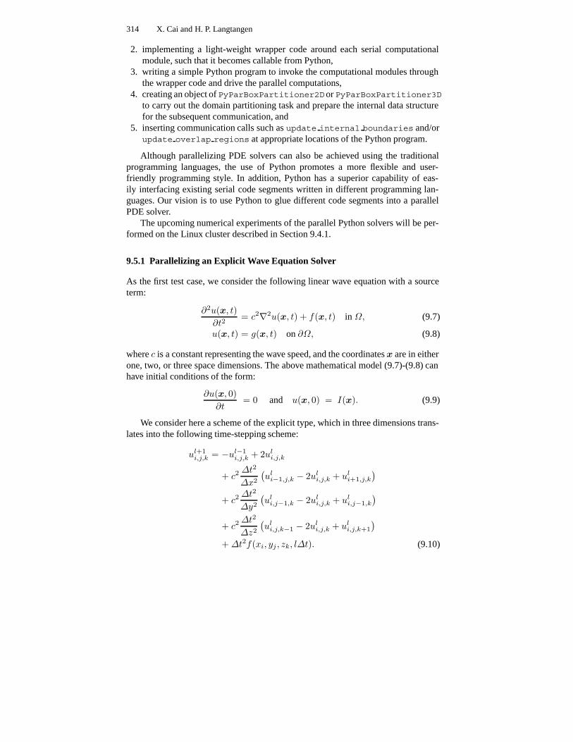
9.5.1 Parallelizing an Explicit Wave Equation Solver

As the first test case, we consider the following linear wave equation with a sourceterm:

∂2u(x, t)∂t2

= c2∇2u(x, t) + f(x, t) in Ω, (9.7)

u(x, t) = g(x, t) on ∂Ω, (9.8)

where c is a constant representing the wave speed, and the coordinates x are in eitherone, two, or three space dimensions. The above mathematical model (9.7)-(9.8) canhave initial conditions of the form:

∂u(x, 0)∂t

= 0 and u(x, 0) = I(x). (9.9)

We consider here a scheme of the explicit type, which in three dimensions trans-lates into the following time-stepping scheme:

ul+1i,j,k = −ul−1

i,j,k + 2uli,j,k

+ c2 ∆t2

∆x2

(ul

i−1,j,k − 2uli,j,k + ul

i+1,j,k

)+ c2 ∆t2

∆y2

(ul

i,j−1,k − 2uli,j,k + ul

i,j−1,k

)+ c2 ∆t2

∆z2

(ul

i,j,k−1 − 2uli,j,k + ul

i,j,k+1

)+ ∆t2f(xi, yj , zk, l∆t). (9.10)

9 Parallel PDE Solvers in Python 315

Here, we have assumed that the superscript l indicates the time level and the sub-scripts i, j, k refer to a uniform spatial computational mesh with constant cell lengths∆x, ∆y, and ∆z.

The Serial Wave Solver

A serial solver has already been programmed in C, where the three-dimensional com-putational module works at each time level as follows:

pos = offset0+offset1; /* skip lower boundary layer (in x)*/for (i=1; i<nx; i++) for (j=1; j<ny; j++)

for (k=1; k<nz; k++) ++pos;u[pos] = -um2[pos] + 2*um[pos] +Cx2*(um[pos-offset0] - 2*um[pos] + um[pos+offset0]) +Cy2*(um[pos-offset1] - 2*um[pos] + um[pos+offset1]) +Cz2*(um[pos-1] - 2*um[pos] + um[pos+1]) +dt2*source3D(x[i], y[j], z[k], t_old);

pos += 2; /* skip the two boundary layers (in z)*/

pos += 2*offset1; /* skip the two boundary layers (in y)*/

Here, the arrays u, um, and um2 refer to u l+1, ul, ul−1, respectively. For the purposeof computational efficiency, each conceptually three-dimensional array actually usesthe underlying data structure of a long one-dimensional array. This underlying datastructure is thus utilized in the above three-level nested for-loop, where we haveoffset0=(ny+1)*(nz+1) and offset1=nz+1. The variables Cx2, Cy2, Cz2, dt2contain the constant values c2∆t2/∆x2, c2∆t2/∆y2, c2∆t2/∆z2, and ∆t2, respec-tively.

Parallelization

Regarding the parallelization, the array-level approach presented in Section 9.3.2applies directly to this type of explicit finite difference schemes. The main modifi-cations of the serial code involve (1) the global computational mesh is divided intoa P = Nx × Ny or P = Nx × Ny × Nz lattice, (2) each processor only constructsits local array objects including ghost points on the internal boundary, and (3) dur-ing each time step, a communication procedure for updating the internal boundaryvalues is carried out after the serial computational module is invoked.

We show in the following the main content of a parallel wave solver implementedin Python:

from BoxPartitioner import *# read ’gnum_cells’ & ’parts’ from command line ...partitioner=PyParBoxPartitioner3D(my_id=my_id,

num_procs=num_procs,global_num_cells=gnum_cells,

316 X. Cai and H. P. Langtangen

Table 9.2. A comparison of the two-dimensional performance between a mixed Python-Cimplementation and and pure C implementation. The global mesh has 2000× 2000 cells (i.e.,2001 × 2001 points) and there are 5656 time steps.

Mixed Python-C Pure CP Wall-time Speedup Wall-time Speedup1 2137.18 N/A 1835.38 N/A2 1116.41 1.91 941.59 1.954 649.06 3.29 566.34 3.248 371.98 5.75 327.98 5.6012 236.41 9.04 227.55 8.0716 193.83 11.03 175.18 10.48

num_parts=parts,num_overlaps=[1,1,1])

partitioner.prepare_communication ()loc_nx,loc_ny,loc_nz = partitioner.get_num_loc_cells ()# create the subdomain data arrays u, um, um2 ...# enforce the initial conditions (details skipped)

import cloopst = 0.0while t <= tstop:

t_old = t; t += dtu = cloops.update_interior_pts3D(u,um,um2,x,y,z,

Cx2,Cy2,Cz2,dt2,t_old)

partitioner.update_internal_boundaries (u)# enforce boundary condition where needed ...tmp = um2; um2 = um; um = u; u = tmp;

Note that the get num loc cells method of class BoxPartitioner returns thenumber of local cells for each subdomain. The cloops.update interior pts3D

call invokes the serial three-dimensional computational module written in C. We alsoassume that the C computational module is placed in a file named cloops.c, whichalso contains the wrapper code needed for accessing the Python data structures in C.For more details we refer to [1].

Large-Scale Simulations

A two-dimensional 2000×2000 mesh and a three-dimensional 200×200×200meshare chosen for testing the parallel efficiency of the mixed Python-C wave equationsolver. For each global mesh, the value of P is varied between 1 and 16, and parallelsimulations of the model problem (9.7)-(9.9) are run on P processors. Tables 9.2 and9.3 report the wall-clock time measurements (in seconds) of the entire while-loop,i.e., the time-stepping part of solving the wave equation. We remark that the numberof time steps is determined by the global mesh size, independent of P .

It can be observed from both tables that the mixed Python-C implementation isof approximately the same speed as the pure C implementation. The speed-up re-sults of the two-dimensional mixed Python-C implementation scale slightly better

9 Parallel PDE Solvers in Python 317

Table 9.3. A comparison of performance between a mixed Python-C implementation anda pure C implementation for simulations of a three-dimensional wave equation. The globalmesh has 200 × 200 × 200 cells and there are 692 time steps.

Mixed Python-C Pure CP Wall-time Speedup Wall-time Speedup1 735.89 N/A 746.96 N/A2 426.77 1.72 441.51 1.694 259.84 2.83 261.39 2.868 146.96 5.01 144.27 5.1812 112.01 6.57 109.27 6.8416 94.20 7.81 89.33 8.36

than the pure C implementation. There are at least two reasons for this somewhatunexpected behavior. First, the Python-C implementation has a better computation-communication ratio, due to the overhead of repeatedly invoking a C function and ex-ecuting the while-loop in Python. We note that this type of overhead is also presentwhen P = 1. Regarding the overhead associated only with communication, we re-mark that it consists of three parts: preparing outgoing messages, message exchange,and extracting incoming messages. The larger latency value of pypar-MPI than thatof C-MPI thus concerns only the second part, therefore it may have an almost invisi-ble impact on the overall performance. In other words, care should be taken to imple-ment the message preparation and extraction work efficiently, and the index slicingfunctionality of Python arrays clearly seems to have sufficient efficiency for thesepurposes. Second, the better speed-up results of the mixed Python-C implementationmay sometimes be attributed to the cache effects. To understand this, we have to re-alize that any mixed Python-C implementation always uses (slightly) more memorythan its pure C counterpart. Consequently, the mixed Python-C implementation hasa better chance of letting bad cache use “spoil” its serial (P = 1) performance, andit will thus in some special cases scale better when P > 1.

We must remark that the relatively poor speed-up results in Table 9.3, forboth pure C and mixed Python-C implementations, are due to the relatively smallcomputation-communication ratio in these very simple three-dimensional simula-tions, plus the use of blocking MPI send/receive routines [11]. For P = 1 in par-ticular, the better speed of the mixed Python-C implementation is due to a fast one-dimensional indexing scheme of the data in the cloop.update interior pts3D

function (which is migrated to C), as opposed to the relatively expansive triple in-dexing scheme (such as u[i][j][k]) in the pure C implementation. The relativelyslow communication speed of the Linux cluster also considerably affects the scala-bility. Non-blocking communication routines can in principle be used for improvingsuch simple parallel simulations. For example, in the pure C implementation, rou-tines such as MPI Isend and MPI Irecv may help to overlap communication withcomputation and thus hide the overhead of communication. At the moment of thiswriting, the pypar package has not implemented such non-blocking communicationroutines, whereas pyMPI has non-blocking communication routines but with rela-

318 X. Cai and H. P. Langtangen

tively slow performance. On the other hand, measurements in Table 9.3 are meant toprovide an accurate idea of the size of the Python-induced communication overhead,so we have deliberately sticked to blocking communication routines in our pure Cimplementations.

9.5.2 Schwarz-Type Parallelization of a Boussinesq Solver

In the preceding case, an explicit finite difference algorithm constitutes the PDEsolver. The parallelization is thus carried out at the array level, see Section 9.3.2.To demonstrate a case of parallelizing a PDE solver at a higher level, as discussedin Section 9.3.3, let us consider the parallelization of an implicit PDE solver imple-mented in a legacy Fortran 77 code. The original serial code consists of loop-basedsubroutines, which heavily involve low-level details of array indexing. It was devel-oped 15 years ago without any paying attention to parallelization. Thus, this casestudy shows how the new Python class hierarchy BoxPartitioner can help to im-plement a Schwarz-type parallelization of old legacy codes.

The choice of the Schwarz-type approach for this case is motivated by two fac-tors. First, the serial numerical scheme is not straightforward to parallelize using thearray-level approach. Second, which is actually a more important motivation, theSchwarz-type parallelization approach alleviates the need of having to completelyunderstand the low-level details of the internal loops and array indexing in the old-style Fortran code.

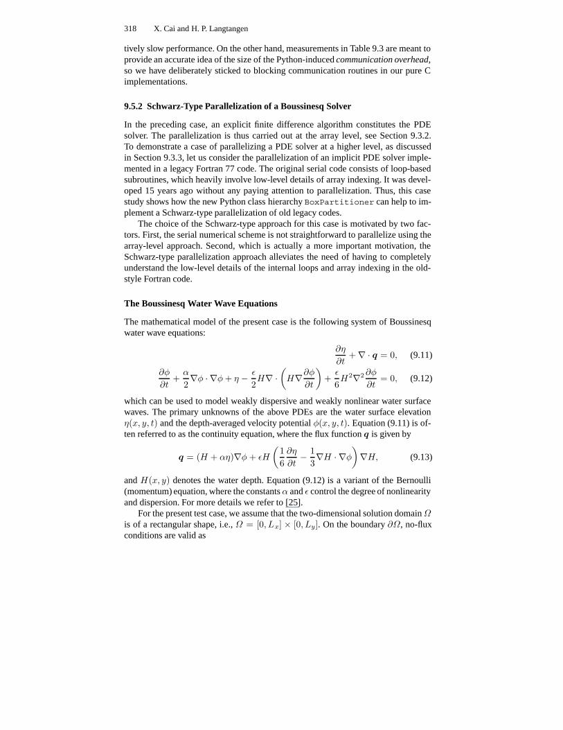
The Boussinesq Water Wave Equations

The mathematical model of the present case is the following system of Boussinesqwater wave equations:

∂η

∂t+ ∇ · q = 0, (9.11)

∂φ

∂t+

α

2∇φ · ∇φ + η − ε

2H∇ ·

(H∇∂φ

∂t

)+

ε

6H2∇2 ∂φ

∂t= 0, (9.12)

which can be used to model weakly dispersive and weakly nonlinear water surfacewaves. The primary unknowns of the above PDEs are the water surface elevationη(x, y, t) and the depth-averaged velocity potential φ(x, y, t). Equation (9.11) is of-ten referred to as the continuity equation, where the flux function q is given by

q = (H + αη)∇φ + εH

(16

∂η

∂t− 1

3∇H · ∇φ

)∇H, (9.13)

and H(x, y) denotes the water depth. Equation (9.12) is a variant of the Bernoulli(momentum) equation, where the constants α and ε control the degree of nonlinearityand dispersion. For more details we refer to [25].

For the present test case, we assume that the two-dimensional solution domain Ωis of a rectangular shape, i.e., Ω = [0, Lx] × [0, Ly]. On the boundary ∂Ω, no-fluxconditions are valid as

9 Parallel PDE Solvers in Python 319

q · n = 0 and ∇φ · n = 0, (9.14)

where n denotes as usual the outward unit normal on ∂Ω. In addition, the Boussi-nesq equations are supplemented with initial conditions in the form of prescribedη(x, y, 0) and φ(x, y, 0).

The Numerical Scheme

As a concrete case of applying the Schwarz-type parallelization approach, we con-sider an old serial legacy Fortran 77 code that uses a semi-implicit numerical schemebased on finite differences. Most of the parallelization effort involves using the F2PYtool to automatically generate wrapper code of the Fortran subroutines and callingmethods of PyParBoxPartitioner2D for the needed communication operations.It should be noted that other implicit numerical schemes can also be parallelized inthe same approach. We refer to [12, 6] for another example of an implicit finite ele-ment numerical scheme, which has been parallelized on the basis of additive Schwarziterations.

The legacy code adopts a time stepping strategy for uniform discrete time levels∆t, ≥ 1, and the temporal discretization of (9.11)-(9.12) is as follows:

η − η−1

∆t+ ∇ ·

((H + α

η−1 + η

2

)∇φ−1+

εH

(16

η − η−1

∆t− 1

3∇H · ∇φ−1

)∇H

)= 0,(9.15)

φ − φ−1

∆t+

α

2∇φ−1 · ∇φ−1 + η − ε

2H∇ ·

(H∇

(φ − φ−1

∆t

))+

ε

6H2∇2

(φ − φ−1

∆t

)= 0.(9.16)

Moreover, by introducing an intermediate solution field FT (note that FT is a singleentity, not F times T ),

FT ≡ φ − φ−1

∆t, such that FT

i,j ≈ ∂φ

∂t(i∆x, j∆y, l∆t), (9.17)

we can simplify the discretized Bernoulli equation (9.16) as

FT − ε

2H∇ · (H∇FT ) +

ε

6H2∇2FT = −α

2∇φ−1 · ∇φ−1 − η.(9.18)

In other words, the computational work of the numerical scheme at time level consists of the following sub-steps:

1. Solve (9.15) with respect to η using η−1 and φ−1 as known quantities.2. Solve (9.18) with respect to FT using η and φ−1 as known quantities.3. Update the φ solution by

φ = φ−1 + ∆t FT . (9.19)

320 X. Cai and H. P. Langtangen

We note that the notation FT arises from the corresponding variable name used inthe legacy Fortran code.

By a standard finite difference five-point stencil, the spatial discretization of(9.15)-(9.18) will give rise to two systems of linear equations:

Aη(φ−1)η = bη(η−1, φ−1), (9.20)

AFT FT = bFT (η, φ−1). (9.21)

The η vector contains the approximate solution of η at (i∆x, j∆y, l∆t), while theFT vector contains the approximate solution of ∂φ/∂t at t = ∆t. The entriesof matrix Aη depend on the latest φ approximation, whereas matrix AFT remainsunchanged throughout the entire time-stepping process. The right-hand side vectorsbη and bFT depend on the latest η and φ approximations.

Parallelization

The existing serial Fortran 77 code uses the line-version of SSOR iterations to solvethe linear systems (9.20) and (9.21). That is, all the unknowns on one mesh line areupdated simultaneously, which requires solving a tridiagonal linear system per meshline (in both x- and y-direction). Such a serial numerical scheme is hard to parallelizeusing the array-level approach (see Section 9.3.2). Therefore, we adopt the Schwarz-type parallelization approach from Section 9.3.3, which in this case means that thesubdomain solver needed in (9.6) invokes one or a few subdomain line-version SSORiterations embedded in the legacy Fortran 77 code.

A small extension of the Fortran 77 code is necessary because of the involvementof the artificial boundary condition (9.6) on each subdomain. However, this extensionis not directly programmed into the old Fortran subroutines. Instead, two new “wrap-per” subroutines, iteration continuity and iteration bernoulli, are writ-ten to handle the discretized continuity equation (9.15) and the discretized Bernoulliequation (9.18), respectively. These two wrapper subroutines use F2PY and are verylight-weight in the sense that they mainly invoke the existing old Fortran subroutinesas “black boxes”. The only additional work in the wrapper subroutines is on testingwhether some of the four side neighbors are absent. For each absent side neighbor,the original physical boundary conditions (9.14) must be enforced. Otherwise, thecommunication method update overlap regions takes care of enforcing the ar-tificial Dirichlet boundary condition required in (9.6).

The resulting parallel Python program runs additive Schwarz iterations at a highlevel for solving both (9.20) and (9.21) at each time level. In a sense, the Schwarzframework wraps the entire legacy Fortran 77 code with a user-friendly Python in-terface. The main content of the Python program is as follows:

from BoxPartitioner import *# read in ’gnum_cells’,’parts’,’overlaps’ ...partitioner=PyParBoxPartitioner2D(my_id=my_id,

num_procs=num_procs,global_num_cells=gnum_cells,

9 Parallel PDE Solvers in Python 321

num_parts=parts,num_overlaps=overlaps)

partitioner.prepare_communication ()loc_nx,loc_ny = partitioner.get_num_loc_cells ()# create subdomain data arrays ...# enforce initial conditions ...

lower_x_neigh = partitioner.lower_neighbors[0]upper_x_neigh = partitioner.upper_neighbors[0]lower_y_neigh = partitioner.lower_neighbors[1]upper_y_neigh = partitioner.upper_neighbors[1]

import BQ_solver_wrapper as f77 # interface to legacy code

t = 0.0while t <= tstop:

t += dt

# solve the continuity equation:dd_iter = 0not_converged = Truenbit = 0

while not_converged and dd_iter < max_dd_iters:dd_iter++Y_prev = Y.copy() # remember old eta valuesY, nbit = f77.iteration_continuity (F, Y, YW, H,

QY, WRK, dx, dy, dt, kit,ik, gg, alpha, eps, nbit,lower_x_neigh, upper_x_neigh,lower_y_neigh, upper_y_neigh)

# communicationpartitioner.update_overlap_regions (Y)not_converged = check_convergence (Y, Y_prev)

# solve the Bernoulli equation:dd_iter = 0not_converged = Truenbit = 0

while not_converged and dd_iter < max_dd_iters:dd_iter++FT_prev = FT.copy() # remember old FT valuesFT, nbit = f77.iteration_bernoulli (F, FT, Y, H,

QR,R,WRK, dx, dy, dt, ik,alpha, eps, nbit,lower_x_neigh, upper_x_neigh,lower_y_neigh, upper_y_neigh)

# communicationpartitioner.update_overlap_regions (FT)not_converged = check_convergence (FT, FT_prev)

F += dt*FT # update the phi field

The interface to the Fortran wrapper code is imported by the statement

import BQ_solver_wrapper as f77

322 X. Cai and H. P. Langtangen

The code above shows that a large number of NumPy arrays and other parameters aresent as input arguments to the two wrapper subroutines iteration continuity

and iteration bernoulli. The arrays are actually required by the old Fortransubroutines, which are used as “black boxes”. The large number of input argumentsshows a clear disadvantage of old-fashion Fortran programming. In particular, thearrays Y, FT, and F contain the approximate solutions of η, FT , and φ, respectively.The other arrays contain additional working data, and will not be explained here. TheIDs of the four side neighbors, lower x neigh, upper x neigh, lower y neigh,and upper y neigh, are also sent in as the input arguments. These neighbor IDs areneeded in the the wrapper subroutines for deciding whether to enforce the originalphysical boundary conditions on the four sides. We also note that the input/outputargument nbit (needed by the existing old Fortran subroutines) is an integer accu-mulating the total number of line-version SSOR iterations used so far in each loopof the additive Schwarz iterations.

To test the convergence of the additive Schwarz iterations, we have coded a sim-ple Python method check convergence. This method compares the relative differ-ence between xs,k and xs,k−1. More precisely, convergence is considered achievedby the kth additive Schwarz iteration if

maxs

‖xs,k − xs,k−1‖‖xs,k‖

≤ ε. (9.22)

Note that a collective communication is needed in check convergence. In (9.22)ε denotes a prescribed convergence threshold value.

Measurements

We have chosen a test problem with α = ε = 1 and

Lx = Ly = 10, H = 1, φ(x, y, 0) = 0, η(x, y, 0) = 0.008 cos(3πx) cos(4πy).

The global uniform mesh is chosen as 1000 × 1000, and the time step size is ∆t =0.05 with the end time equal to 2. The number of overlapping cell layers between theneighboring subdomains has been chosen as 8. One line-version SSOR iteration isused as the subdomain solver associated with solving (9.15), and three line-versionSSOR iterations are used as the subdomain solver associated with solving (9.18). Theconvergence threshold value for testing the additive Schwarz iterations is chosen asε = 10−3 in (9.22).

We remark that the legacy Fortran code is very difficult to parallelize in a pureFortran manner, i.e., using the array-level approach. Therefore, the performance ofthe Schwarz-type parallel Python-Fortran solver is not compared with a “reference”parallel Fortran solver, but only studied by examining its speed-up results in Ta-ble 9.4. It can be seen that Table 9.4 has considerably better speed-up results thanTable 9.2. This is due to two reasons. First, the computation-communication ratio islarger when solving the Boussinesq equations, because one line-version SSOR itera-tion is more computation-intensive than one iteration of a seven-point stencil, which

9 Parallel PDE Solvers in Python 323

Table 9.4. The wall-time measurements of the parallel Python Boussinesq solver. The globaluniform mesh is 1000× 1000 and the number of time steps is 40. The number of overlappingcell layers between neighboring subdomains is 8.

P Partitioning Wall-time Speed-up1 N/A 1810.69 N/A2 1 × 2 847.53 2.144 2 × 2 483.11 3.756 2 × 3 332.91 5.448 2 × 4 269.85 6.71

12 3 × 4 187.61 9.6516 2 × 8 118.53 15.28

is used for the three-dimensional linear wave equation. Second, allocating a largenumber of data arrays makes the Boussinesq solver less cache-friendly than the lin-ear wave solver for P = 1. This explains why there is a superlinear speed-up fromP = 1 to P = 2 in Table 9.4. These two reasons thus have a combined effect formore favorable speed-up results, in spite of the considerable size of the overlap zone(8 layers).

9.6 Summary

It is well known that Python handles I/O, GUI, result archiving, visualization, reportgeneration, and similar tasks more conveniently than the low-level languages likeFortran and C (and even C++). We have seen in this chapter the possibility of usinghigh-level Python code for invoking inter-processor communications. We have alsoinvestigated the feasibility of parallelizing serial PDE solvers with the aid of Python,which is quite straightforward due to easy re-use of existing serial computationalmodules. Moreover, the flexible and structured style of Python programming helpsto code the PDE-independent parallelization tasks as generic methods. As an exam-ple, an old serial legacy Fortran 77 code has been parallelized using Python with mi-nor efforts. The performance of the resulting parallel Python solver depends on twothings: (1) good serial performance which can be ensured by the use of NumPy ar-rays, vectorization, and mixed-language implementation, (2) high-performance mes-sage passing and low cost of constructing and extracting data messages, for whichit is important to combine the pypar package with the functionality of array slicingand reshaping. Doing this right, our numerical results show that comparable parallelperformances with respect to pure Fortran/C implementations can be obtained.

Acknowledgement. The authors would like to thank Prof. Geir Pedersen at the Department ofMathematics, University of Oslo, for providing access to the Fortran Boussinesq legacy codeand guidance on the usage.

324 X. Cai and H. P. Langtangen

References

1. D. Ascher, P. F. Dubois, K. Hinsen, J. Hugunin, and T. Oliphant. Numerical Python.Technical report, Lawrence Livermore National Lab., CA, 2001.http://www.pfdubois.com/numpy/numpy.pdf.

2. D. L. Brown, W. D. Henshaw, and D. J. Quinlan. Overture: An object-oriented frame-work for solving partial differential equations. In Y. Ishikawa, R. R. Oldehoeft, J. V. W.Reynders, and M. Tholburn, editors, Scientific Computing in Object-Oriented ParallelEnvironments, Lecture Notes in Computer Science, vol 1343, pages 177–184. Springer,1997.

3. A. M. Bruaset, X. Cai, H. P. Langtangen, and A. Tveito. Numerical solution of PDEson parallel computers utilizing sequential simulators. In Y. Ishikawa, R. R. Oldehoeft,J. V. W. Reynders, and M. Tholburn, editors, Scientific Computing in Object-OrientedParallel Environments, Lecture Notes in Computer Science, vol 1343, pages 161–168.Springer, 1997.

4. X. Cai and H. P. Langtangen. Developing parallel object-oriented simulation codes inDiffpack. In H. A. Mang, F. G. Rammerstorfer, and J. Eberhardsteiner, editors, Proceed-ings of the Fifth World Congress on Computational Mechanics, 2002.

5. X. Cai, H. P. Langtangen, and H. Moe. On the performance of the Python program-ming language for serial and parallel scientific computations. Scientific Programming,13(1):31–56, 2005.

6. X. Cai, G. K. Pedersen, and H. P. Langtangen. A parallel multi-subdomain strategy forsolving Boussinesq water wave equations. Advances in Water Resources, 28(3):215–233,2005.

7. T. F. Chan and T. P. Mathew. Domain decomposition algorithms. In Acta Numerica 1994,pages 61–143. Cambridge University Press, 1994.

8. D. B. et al. Swig 1.3 Development Documentation, 2004. http://www.swig.org/doc.html.

9. F2PY software package. http://cens.ioc.ee/projects/f2py2e.10. L. Formaggia, M. Sala, and F. Saleri. Domain decomposition techniques. In A. M.

Bruaset, P. Bjørstad, and A. Tveito, editors, Numerical Solution of Partial DifferentialEquations on Parallel Computers, volume X of Lecture Notes in Computational Scienceand Engineering. Springer-Verlag, 2005.

11. M. P. I. Forum. MPI: A message-passing interface standard. Internat. J. SupercomputerAppl., 8:159–416, 1994.

12. S. Glimsdal, G. K. Pedersen, and H. P. Langtangen. An investigation of domain decom-position methods for one-dimensional dispersive long wave equations. Advances in WaterResources, 27(11):1111–1133, 2005.

13. C. Hughes and T. Hughes. Parallel and Distributed Programming Using C++. AddisonWesley, 2003.

14. H. P. Langtangen. Python Scripting for Computational Science. Texts in ComputationalScience and Engineering, vol 3. Springer, 2004.

15. H. P. Langtangen and X. Cai. A software framework for easy parallelization of PDEsolvers. In C. B. Jensen, T. Kvamsdal, H. I. Andersson, B. Pettersen, A. Ecer, J. Peri-aux, N. Satofuka, and P. Fox, editors, Parallel Computational Fluid Dynamics. ElsevierScience, 2001.

16. Matlab code vectorization guide.http://www.mathworks.com/support/tech-notes/1100/1109.html.

17. Numerical Python software package.http://sourceforge.net/projects/numpy.

9 Parallel PDE Solvers in Python 325

18. P. S. Pacheco. Parallel Programming with MPI. Morgan Kaufmann Publishers, 1997.19. Parallel software in C and C++.

http://www.mathtools.net/C_C__/Parallel/.20. R. Parsones and D. Quinlan. A++/P++ array classes for architecture independent finite

difference computations. Technical report, Los Alamos National Lab., NM, 1994.21. PyMPI software package. http://sourceforge.net/projects/pympi, 2004.22. PyPar software package. http://datamining.anu.edu.au/˜ole/pypar,

2004.23. ScientificPython software package.

http://starship.python.net/crew/hinsen.24. B. F. Smith, P. E. Bjørstad, and W. Gropp. Domain Decomposition: Parallel Multilevel

Methods for Elliptic Partial Differential Equations. Cambridge University Press, 1996.25. D. M. Wu and T. Y. Wu. Three-dimensional nonlinear long waves due to moving surface

pressure. Proc. 14th Symp. Naval Hydrodyn., pages 103–129, 1982.