Numerical diffusive terms in weakly-compressibleSPH schemes

M. Antuono a, A. Colagrossi a,b,∗, S. Marrone a

aCNR-INSEAN, The Italian Ship Model Basin, Rome, ItalybCESOS: Centre of Excellence for Ship and Ocean Structures, NTNU, Trondheim,

Norway

Abstract

A discussion on the use of numerical diffusive terms in SPH models is proposed. Such termsare, generally, added in the continuity equation, in order to reduce the spurious numericalnoise that affects the density and pressure fields in weakly-compressible SPH schemes.Specific focus has been given to the theoretical analysis of the diffusive term structure,highlighting the main benefits and drawbacks of the most widespread formulations. Finally,specific test cases have been used to compare such formulations and to confirm thetheoretical findings.

Key words: Smoothed Particle Hydrodynamics, weak-compressibility, numericaldiffusive terms, free-surface flows

1 Introduction

The Smoothed Particle Hydrodynamics (SPH hereinafter) is a meshless Lagrangianscheme that relies on a smoothing procedure. This enables modeling the spatialdifferential operators through summations over Lagrangian nodes (namely fluidparticles) that carry the flow properties (e.g. pressure, velocity, density etc.). Inthe SPH literature, two principal approaches are used to model liquids: one isbased on the smoothing of the Navier-Stokes equations and on the solution of aPoisson equation for the pressure field (see, for example, [1,2]), the other relies onthe assumption that the fluid is weakly-compressible and barotropic (e.g. [3,4]).

∗ Corresponding author: Tel.: +39 06 50 299 343; Fax: +39 06 50 70 619.Email addresses: m.antuono@insean.it (M. Antuono), a.colagrossi@insean.it

(A. Colagrossi), s.marrone@insean.it (S. Marrone).

Preprint submitted to Elsevier 11 June 2015

Concerning the numerical implementation, the main difference between theweakly-compressible and incompressible approaches is that the former requiressmall time steps, constrained by the speed of sound, while the latter allows forlarger time steps but is difficult to parallelize because it needs to solve an algebraicsystem with a sparse matrix. Generally, weakly-compressible schemes are moresuited for free-surface flows since the boundary condition along the free surfaceis implicitly satisfied (see, for example, Colagrossi et al. [5]). This implies thatthe weakly-compressible schemes do not require an explicit detection of the freesurface during the flow evolution. The latter issue is of crucial importance for 3Dsimulations of violent flows since the Poisson equation (used in incompressibleschemes) may strongly depend on the free-surface configuration and small errorsin the free-surface detection can lead to different flow dynamics.

Unfortunately, weakly-compressible schemes have, as a major drawback, thegeneration of spurious numerical oscillations in the pressure and density fields. Toremove/reduce the spurious numerical noise, different solutions have been proposedover the years.

Monaghan and Gingold [6] introduced an artificial viscous term based on aNeumann-Richtmeyer artificial viscosity to dampen the oscillations appearing inshock waves. Such an artificial viscosity term also helped stabilize the SPH schemeand reduce spurious oscillations.

In Colagrossi & Landrini [7] the authors suggested to filter the density field througha Mean Least Square (MLS) integral interpolation. This procedure gave goodresults, but, for long-time simulations, it did not conserve the total volume ofthe fluid system since the hydrostatic component was filtered improperly (see e.g.Sibilla [8]).

An alternative approach has been proposed by Vila [9] and by Moussa and Vila[10], who studied the convergence of SPH schemes based on approximate Riemannsolvers and disregarding artificial viscosity. From their works, a family of Riemann-solver SPH schemes has been built. These models, generally, give good results but,unfortunately, do not allow an exact quantification of the dissipations caused by thenumerical scheme, that, in any case, are quite large.

Exploiting the theory of Riemann solvers, Ferrari et al. [11] built a numericaldiffusive term on the basis of a Rusanov flux. This term has been added to thecontinuity equation to reduce the numerical noise inside the density field. Since inthe weakly-compressible schemes the pressure field is evaluated from the densityfield through the state equation (the fluid is assumed to be barotropic), a smootherdensity field corresponds to a smoother pressure field. Use of a numerical diffusiveterm inside the continuity equation has been also proposed by Molteni & Colagrossi[12]. Their term gave good results but, unfortunately, was not compatible with thehydrostatic solution. The authors avoided this issue by introducing a threshold

2

density so that the diffusive term only worked when the pressure exceeded thehydrostatic solution. Unfortunately, this strategy led to a drastic reduction of thediffusive term action. To go round this issue, Antuono et al. [13] proposed acorrection to the diffusive term of Molteni & Colagrossi [12]. This proved to becompatible with the hydrostatic solution and to properly smooth out the numericalspurious oscillations from the pressure and density fields.

The aim of the present work is to shed light on the use of numerical diffusive termsin SPH. Specifically, we focus on the diffusive term of Ferrari et al. [11], Molteni& Colagrossi [12] and Antuono et al. [13] and show their benefits and drawbacks.Section §2 briefly introduces the SPH scheme which includes a numerical diffusiveterm in the continuity equation, while Sections §3 and §4 provide the maintheoretical findings and give details about the time integration scheme. Finally, inSection §5 some specific test cases are used to compare the different diffusive termsand confirm the theoretical analysis.

2 SPH scheme with numerical diffusive terms

In this section we study the general structure of a SPH scheme with a numericaldiffusive term in the continuity equation. Specifically, we assume the fluid tobe weakly-compressible and barotropic. Under these hypotheses, the densityvariations are small and it is possible to linearize the state equation in theneighborhood of the reference density to get a linear dependence of the pressureon the density field. Finally, the artificial viscous term by Monaghan & Gingold [6]is added in the momentum equation for stability reasons. In any case, we underlinethat the theoretical analysis on the role of the diffusive term is completely generaland can be applied to SPH schemes with different features.

Under the hypotheses made above, the governing equations for the SPH scheme athand are:

Dρi

Dt= − ρi

∑j

(u j − ui) · ∇iWi j V j + δ h c0Di (2.1a)

Dui

Dt= −

1ρi

∑j

(p j + pi)∇iWi j V j + f i + α h c0ρ0

ρi

∑j

πi j ∇iWi j V j (2.1b)

Dri

Dt= ui pi = c2

0 ( ρi − ρ0 ) (2.1c)

where ρi, Vi, pi are respectively the density, the volume and the pressure of the i−thparticle while ri and ui are its position and velocity. Here, Wi j is the kernel functionand depends on q = ‖r j − ri‖/h, ∇i denotes the differentiation with respect to ri

and f i is the body force at the position ri. Finally, symbols ρ0 and c0 indicate thedensity along the free surface (which is the reference value for the density field)

3

and the sound velocity (assumed to be constant). For computational reasons, itis common practice in weakly-compressible SPH solvers not to use the physicalsound velocity but to impose c0 to be at least one order of magnitude greater than themaximum flow velocity, that is, c0 ≥ 10 maxi ui. As pointed out by Monaghan [14],this assumption ensures the density variations to remain below 1%. In presence ofgravity waves a more restrictive constraint has to be used on the choice of the speedof sound (for details see [15], [16]).

In this scheme, the diffusive term is briefly indicated byDi [equation (2.1a)] and ismultiplied by a dimensionless coefficient, δ, whose range of variability is inspectedin Section §3.1. The diffusive term has the dimension of the Laplacian of ρ. Theartificial viscosity term is the last term in (2.1b). Its argument is

πi j =(u j − ui) · r ji

‖r ji‖2 (2.2)

where r ji = r j − ri. For incompressible flows, Español & Revenga [18] provedthat the artificial viscous term approximates ν∇2u where ν is the kinetic viscosity.Specifically, ν = αhc0/(4 + 2 n) and n is the number of spatial dimensions (see [14]for details).

For the analysis which follows, it is useful to study the convergence of the pressuregradient operator in (2.1b). Using the results of Colagrossi et al. [5] on thesmoothed SPH operators, we can rewrite it as follows:∑

j

(p j + pi)∇iWi j V j =∑

j

(p j − pi)∇iWi j V j + 2 p1

∑j

∇iWi j V j =

= Γi ∇pi + 2 pi ∇Γi + O(h) , (2.3)

where:

Γi =∑

j

Wi j V j ∇Γi =∑

j

∇iWi j V j . (2.4)

As discussed in Colagrossi et al. [5], Γi ' 1 and ∇Γi ' 0 inside the fluid domain.On the contrary, near the free surface Γi is no more constant and ∇Γi points towardsthe interior of the fluid domain and diverges like 1/h. In this case, the convergenceof the differential operator is ensured by assigning p = 0 along the free surface.Because of (2.3), the overall contribution of the pressure gradient to the momentumequation is:

Dui

Dt= −

Γi

ρi∇pi −

2 pi

ρi∇Γi + . . . (2.5)

The last term on the right-hand side of (2.5) plays a relevant role when the diffusiveterm is included in the continuity equation. This is analyzed in the followingsection.

4

2.1 Diffusive terms

In the SPH literature, different diffusive terms have been defined. Generally, theycan be reduced to the following structure:

Di = 2∑

j

ψ jir ji · ∇iWi j

‖r ji‖2 V j (2.6)

where ψ ji changes according to the specific formulation at hand and has thephysical dimension of the density. In order to be a diffusive term, the expressionin (2.6) has to approximate even derivatives of the density/pressure field. Further,for consistency with the global equation of the mass conservation, the diffusiveterm must satisfy: ∑

i

Di Vi = 0 ⇔ ψ ji = −ψi j . (2.7)

The simplest approach to artificial diffusion in SPH is that of Molteni & Colagrossi[12] who added the Laplacian of the density field in the continuity equation. Thisis equivalent to:

ψMolji = ρ j − ρi (2.8)

As shown in Antuono et al. [13], use of (2.8) into (2.6) leads to:

DMoli = 2∇ρi · ∇Γi + Γi ∇

2ρi + O(h) . (2.9)

The second term on the right-hand side of (2.9) contains second-order derivativesand, therefore, represents a diffusive term. Conversely, the first term on the right-hand side is a first-order differential operator. Inside the fluid bulk, Γi ' 1,∇Γi ' 0 and, consequently, the first-order differential operator is null and DMol

iapproximates the Laplacian of the density field.

Conversely, the behavior of DMoli drastically changes close to the free surface.

There, ∇Γi is non-zero and points toward the fluid region. If the fluid is close tothe hydrostatic condition, the density gradient points in the same direction and,consequently, ∇ρi · ∇Γi is positive. Since this is the leading term in (2.9), DMol

i ispositive as well. Through equation (2.1a), DMol

i causes an increase of the densityalong the free surface and a subsequent increase of the pressure field because of thestate equation. In turn, this implies that the term (−pi∇Γi) in (2.5) is no longer zeroand acts as a force directed towards the outside of the fluid body. Because of thisphenomenon, the particles start moving upwards and do not satisfy the hydrostaticsolution.

A correction to the formula of Molteni & Colagrossi [12] has been proposed byAntuono et al. [13]. This formula is convergent all over the fluid domain, preserves

5

exactly the conservation of mass and satisfies the hydrostatic solution. It reads:

ψAnji =

(ρ j − ρi

)−

12

(〈∇ρ〉Lj + 〈∇ρ〉Li

)· r ji

(2.10)

The symbol 〈∇ρ〉Li indicates the renormalized density gradient [17] defined as:

〈∇ρ〉Li =∑

j

(ρ j − ρi) Li ∇iWi j V j ;

Li =

[∑j

(r j − ri) ⊗ ∇iWi j V j

]−1 (2.11)

Another interesting approach to diffusion has been derived by Ferrari et al. [11]on the basis of a Rusanof flux. Assuming that the sound velocity is constant, theirdiffusive term reduces to:

ψFeji =

(ρ j − ρi)2 h

‖r ji‖ . (2.12)

Remarkably, the SPH scheme defined by Ferrari et al.[11] neither needs anytuning of δ (which is set equal to 1) nor use of artificial viscosity to stabilizethe scheme. Notwithstanding this, such a term still leads to a positive contributionin the continuity equation which makes the attainment of the hydrostatic solutionimpossible. This is proved in the following sections along with an accurate analysisof the diffusive term proposed by Ferrari et al. [11] and by Antuono et al. [13].

3 Convergence of the diffusive operators

Here we deal with the convergence of the diffusive terms described in Section §2.1while we postpone the analysis of the diffusive coefficient δ to Section §3.1. Tosimplify the discussion, we make an analysis at the continuum by substituting thesummations over the fluid particles with integrals over the kernel domain Ω. Inthis context, we denote by r and r′ two points in the fluid domain and all thequantities evaluated at r′ are indicated through the superscript “prime” (i.e., f ′

indicates f (r′)). For the ease of the notation, we also define q = (r′ − r)/h andq = ‖q‖ while the subscripts k, l,m, n denote the components of vectors/tensors. Asa consequence, the kernel gradient can be rewritten as follows:

W = W(q) ⇒ ∇W = −1h

qq∂W∂q

, (3.13)

6

and the structure of diffusive term in (2.6) becomes:

D = −2h2

∫Ω

ψ

q∂W∂q

dV ′ . (3.14)

First, we consider the expression by Ferrari et al. [11]. As proved in appendix A,the following expansion holds true:

DFe = ∇ρ ·

∫Ω

q ∇W dV ′ +12H(ρ) :

∫Ω

q (r′ − r) ⊗ ∇W dV ′ + O(h) , (3.15)

whereH is the Hessian of ρ. From symmetry properties, the first term on the right-hand side is null inside the fluid domain while close to the free surface is non-zeroand is directed towards the interior of the fluid region. Similarly to term ∇ρ · ∇Γ ofequation (2.9), this leads to a positive contribution in the continuity equation andimplies the impossibility to attain the hydrostatic solution. Because of the similarityof the diffusive term of Molteni & Colagrossi [12] with that of Ferrari et al. [11],hereinafter we mainly focus on the latter one.

As proved in appendix A, the diffusive term by Antuono et al. [13] converges tozero for h going to zero. Its main contributions are:

DAn =h6

(∂3ρ

∂rk∂rl∂rm

) ∫Ω

qk ql qm

q∂W∂q

dV ′ +

+h2

12

(∂4ρ

∂rk∂rl∂rm∂rn

) ∫Ω

qk ql qm qn

q∂W∂q

dV ′ + O(h3) (3.16)

where qk = (r′k − rk)/h is the k−th component of q. For symmetry reasons, thefirst term on the right-hand side is null inside the fluid domain. On the contrary,it is generally non-zero near the free surface even if it maintains very small. Thediffusive term has no influence on the hydrostatic solution. In fact, since the stateequation of system (2.1) is linear, the hydrostatic solution predicts a density fieldthat is a linear function of r. Consequently, this impliesDAn = 0.

The presence of third- and fourth-order derivatives in (3.16) ensures that thediffusive term acts only when short-scale variations/fluctuations of the density fieldoccur. As a consequence, it smooths out the spurious numerical high-frequencyoscillations inside the pressure field without affecting the actual solution.

3.1 Linear stability analysis

Here we provide the one-dimensional linear stability analysis for the SPH schemewith the diffusive term proposed by Antuono et al. [13]. This enables inspectionof the range of variability of the diffusive coefficient, δ. Similar to what was donein the previous section, the analysis is performed at the continuum level, that is,

7

using the continuous differential operators which are approximated by the discretesummations in system (2.1). To do this, we neglect the action of the free surfaceand take the limit for h going to zero. Under these hypotheses, the convergence ofthe SPH differential operators is given by Español & Revenga [18]. These allowrewriting system (2.1) into the following continuous form:

DρDt

= − ρ∇ · u + δ h c0D ,

DuDt

= −∇pρ

+ 2 ν∇ (∇ · u) + ν∇2u

p = c20 (ρ − ρ0) ,

(3.17)

which corresponds to a weakly-compressible version of the Navier-Stokesequations with a diffusive term in the continuity equations.

Let us consider the linearized one-dimensional form of system (3.17) and use thediffusive term of Antuono et al. [13]. In one dimension ν = αhc0/6 (see, forexample, Monaghan & Gingold [6]) while the diffusive term can be rewritten as:

DAn = − h2 Bd4ρ

dx4 (3.18)

where the parameter B depends on the specific kernel function used (see appendixA for more details). Then, system (3.17) becomes:

ρt + ρ0 ux + δ h3 c0 B ρxxxx = 0

ut +c2

0

ρ0ρx −

α h c0

2uxx = 0 .

(3.19)

Let us consider waves in the form of harmonic functions, that is:

ρ = ρ0 + R exp [ i k (x − c t) ] + c.c. u = U exp [ i k (x − c t) ] + c.c. (3.20)

Specifically, R and U indicate the amplitudes of the density and velocity waves,k = 2 π/λ is the wave number, λ is the wave length, c = a + i b where a, b ∈ R and‘c.c.’ denotes the complex conjugate. Specifically, a represents the wave celerityand b is the so-called damping coefficient. If b is negative the solution is stable,otherwise it is unstable.

Substituting (3.20) in (3.19) and using the dimensionless variable µ = k h, weobtain two different regimes for the solution of the linearized equations. The first

8

one is obtained when:

F(µ) = 1 −µ2

4

(α

2− µ2 B δ

)2≥ 0 , (3.21)

and gives:

a(±) = ± c0

√F(µ) b(0) = −

µ c0

2

(α

2+ µ2 B δ

). (3.22)

Conversely, when F(µ) < 0, we find the second regime:

a(0) = 0 b(±) = c0

−µ

2

(α

2+ µ2 B δ

)±

√− F(µ)

(3.23)

In this case, the correct damping rate is given by b(+) since b(−) ≤ b(+) ≤ 0.

Since b is negative in both regimes, this ensures the stability of the δ-SPH scheme.Figure 1 displays a/c0 (dashed line) and b/c0 (solid line) as functions of µ forα = 0.01, δ = 1.0 and B = 1/8 (Gaussian kernel). The damping coefficient b isstrictly decreasing in the first regime, reaches a minimum at the boundary with thesecond regime and, then, becomes an increasing function of µ (here we refer tob(+)). This implies that the occurrence of the second regime is associated with areduced damping of higher frequencies (or equivalently, with a reduced dampingof shorter wave lengths). For this reason, an optimal choice for δ is that ensuringthe occurrence of the first regime, that is, the fulfillment of the condition (3.21).This corresponds to:

1Bµ2

(α

2−

2µ

)≤ δ ≤

1Bµ2

(α

2+

2µ

). (3.24)

Now, we have to define the range of variability of µ. The minimum length of thespurious oscillations in the SPH framework is that corresponding to a sawtoothprofile, that is, λ = 2 ∆x where ∆x is the mean particle distance. Then, themaximum value for µ is given by µ0 = π (h/∆x). For the Gaussian kernel h/∆x =

4/3 and, therefore, µ0 = 4 π/3. Since the upper bound in (3.24) is a strictlydecreasing function of µ while the lower bound has a maximum at µ = 6/α, theexpression (3.24) can be modified to get a sufficient condition for the fulfillment ofcondition (3.21) for all µ ∈ [0, µ0]:

1B

(α

6

)3≤ δ ≤

1Bµ2

0

(α

2+

2µ0

). (3.25)

The expression above is valid for α < 12/µ0 otherwise the lower bound is greaterthan the upper bound. For α = 0 and B = 1/8 (Gaussian kernel), relation (3.25)simply becomes δ ≤ 0.21. Then, to guarantee the occurrence of the first regime, wefix δ = 0.2 in all the numerical simulations that implementDAn.

It is interesting to repeat the above analysis for δ = 0, that is, when only the viscousterm is included in the SPH scheme. In such a case, the linear stability analysis still

9

µ

a/c0

a(−)/c0

a(+)/c0

b/c0

b(+)/c0

b(−)/c0

Fig. 1. Sketch of the regimes predicted by the one-dimensional linear stability analysis:a/c0 (dashed line) and b/c0 (solid line) for α = 0.01, δ = 1.0 and B = 1/8 (Gaussiankernel).

confirms that the solution is stable for each choice of α. Specifically, the condition(3.21) is surely satisfied when:

0 < α <4µ0. (3.26)

Similar to the analysis made for δ , 0, values of α out of the interval in (3.26) leadthe solution in the region of slow damping. The range of variability of α in (3.26) isnarrower than that for the diffusive case (for which 0 < α < 12/µ0). This means thatuse of the diffusive term allows for a more efficient action of the viscosity againstthe numerical spurious oscillations.

4 Integration Scheme

We tested both a third-order TVD Runge-Kutta scheme (see, for example, Gottlieb& Shu [19]) and a classic fourth-order Runge-Kutta scheme. We found that theaccuracy of these schemes was practically equivalent even if the fourth-orderRunge-Kutta scheme proved to be faster than the TVD scheme because of its higherCourant-Friedrick-Lewy (CFL) number. For this reason, the fourth-order Runge-Kutta scheme has been used for the simulations that implement the diffusive termof Antuono et al. [13]. On the contrary, to follow exactly the integration schemeproposed in Ferrari et al. [11], we used the third-order TVD Runge-Kutta schemefor simulations withDFe.

10

For what concerns the fourth-order Runge-Kutta scheme, the diffusive term can beadded directly in all the sub-steps. If we rewrite system (2.1) as follows:

DwDt

= F(w) , (4.27)

the fourth-order Runge-Kutta scheme reads:

w(0) = wn

w(1) = w(0) + F(w(0)) ∆t/2

w(2) = w(0) + F(w(1)) ∆t/2

w(3) = w(0) + F(w(2)) ∆t

w(4) = w(0) +[

F(w(0)) + 2 F

(w(1)) + 2 F

(w(2)) + F

(w(3)) ] ∆t/6

wn+1 = w(4) ,

(4.28)

where the superscripts indicate the time sub-steps. Since the cost of re-evaluatingthe diffusive term at every stage of the scheme is substantial, Jameson et al. [20]proposed a faster scheme to integrate systems with artificial diffusive/dissipativeterms. First, the right-hand side of (4.27) is split as F = Q + D where D containsonly the diffusive term. Then, system (4.27) is integrated through a “frozen”diffusion approach, that is:

w(0) = wn

w(1) = w(0) + Q(w(0)) ∆t/2 + D

(w(0)) ∆t/2

w(2) = w(0) + Q(w(1)) ∆t/2 + D

(w(0)) ∆t/2

w(3) = w(0) + Q(w(2)) ∆t + D

(w(0)) ∆t

w(4) = w(0) +[Q(w(0)) + 2 Q

(w(1)) + 2 Q

(w(2)) + Q

(w(3)) ] ∆t/6 + D

(w(0)) ∆t

wn+1 = w(4) .

(4.29)

Jameson et al. [20] proved this scheme to be robust and reliable. The integrationof the artificial diffusive term is less accurate then the classic fourth-order Runge-Kutta scheme but, in any case, this can be regarded as a minor issue since D doesnot represent a physical diffusion phenomenon.

The last part of the analysis is devoted to the definition of a proper CFL number forthe integration scheme described in (4.29). As shown in appendix A, the diffusiveterm has the following structure in the interior of the fluid bulk:

DAni =

h2

12B jkpq

(∂4ρi

∂r j∂rk∂rp∂rq

), (4.30)

11

where i is the particle index while j, k, p, q are the indexes of the spatial coordinates.Substituting (4.30) in the continuity equation and comparing with Dρi/Dt, it gives:

∆t ≤ CFL(di f f ) hδ c0

. (4.31)

This means that the time step should decrease when the diffusive coefficientincreases. For a fourth-order Runge-Kutta scheme with a Gaussian kernel weheuristically found CFL(di f f ) = 0.44. The global CFL should also account forthe artificial viscosity and for the particle acceleration ai. The time-step boundsderiving from these terms have been modeled following the works of Monaghan& Kos [21] and Morris et al. [22]. They depend on the specific integration schemevery weakly and are given as:

∆t ≤ 0.125h2

ν∆t ≤ 0.25 min

i

√h‖ai‖

, (4.32)

where, according to Monaghan [14], ν = αhc0/(2n + 4) is the kinematic viscosityof the SPH scheme (n is the spatial dimension). Finally, the advective/acousticcomponent of system (2.1) should be accounted for. For a fourth-order Runge-Kuttascheme with a Gaussian kernel we heuristically found:

∆t ≤ 2.2 mini

(h

c0 + ‖ui‖ + h max j πi j

). (4.33)

The global CFL is given as the minimum over all the bounds above.

5 Test cases

In the following sections we provide some numerical simulations that highlight themain features of the diffusive terms mentioned before. Because of the similarityof the diffusive term of Molteni & Colagrossi [12] with that of Ferrari et al. [11],hereinafter we mainly focus on the latter one.

In all the numerical simulations that follow the solid boundaries have been modeledthrough the fixed ghost particle technique (see Marrone et al. [23]) and a free-slipcondition has been imposed. A renormalized Gaussian kernel has been used (see,for example, Landrini et al. [24]).

5.1 Hydrostatic solution

In the present section we deal with a simple hydrostatic problem: a two-dimensionaltank is partially filled with water at rest. Here, L is the tank length and H is

12

Fig. 2. Hydrostatic solution. Left panels: SPH with the diffusive term of Ferrari et al. [11].Right panels: SPH with the diffusive term of Antuono et al. [13].

the filling height. Figure (2) illustrates the comparison between the SPH with thediffusive term of Ferrari et al. [11] and with the diffusive term of Antuono et al.[13] for two spatial resolutions. As expected, in the former case (left panels) thefluid particles tend to move upwards because of the inaccuracy of the diffusiveterm close to the free surface and the hydrostatic solution is completely destroyed.This behavior still persists using a finer resolution even if it slightly decreases inintensity. Conversely, use of the diffusive term of Antuono et al. [13] (right panels)does not alter the correct hydrostatic solution.

A further proof of the unphysical action of the diffusive term of Ferrari et al. [11]is given in figure 3 where the evolution of the potential energy is displayed. Inhydrostatic conditions, the potential energy should be conserved since no motionshould occur. On the contrary, the diffusive term of Ferrari et al. [11] leads to arapid decrease of the initial energy value.

The unphysical motion of the free surface also affects those problems characterized

13

Fig. 3. Hydrostatic solution (H/∆x = 50). Evolution of the potential energy as predictedby the SPH scheme with the diffusive term of Ferrari et al. [11] (dashed line) and with thediffusive term of Antuono et al. [13] (solid line).

Fig. 4. Sketch of the dam-break problem described in Buchner et al.[25]. The symbol P1indicates the pressure probe at the right wall.

by a slow particle motion and a long-time dynamics as, for example, sloshingproblems and gravity wave propagation. Conversely, for more energetic events andshort-time dynamics (as, for example, water jets and impacts), the influence of thespurious terms close to the free surface is much smaller. This is highlighted in thenext test case.

5.2 Dam break

Here we consider the dam break problem studied by Buchner [25]. Figure 4displays a sketch of the configuration: a reservoir is placed at the left side of arectangular basin with water at rest. Then, the right wall of the reservoir is suddenlyremoved and the water starts moving until it impacts against the right wall of thebasin. Along the wall, a probe (indicated by P1) records the pressure signal. Thesketch in figure 4 displays the pressure field just after removal of the right wall ofthe reservoir.

As a first test case, we set α = 0 (that is, no artificial viscosity) and consider

14

Fig. 5. snapshots of the evolution for the dam break problem (α = 0). Top panels: SPHwithout diffusion. Middle panels: SPH with the diffusive term of Ferrari et al. [11]. Bottompanels: SPH with the diffusive term of Antuono et al. [13].

Fig. 6. Evolution of the mechanical energy for the dam break problem with α = 0. SPHwithout diffusion (), SPH with the diffusive term of Ferrari et al. [11] (), SPH with thediffusive term of Antuono et al. [13] (4).

the standard SPH scheme (that is, the SPH model without diffusion) along withthe diffusive formulations of Ferrari et al. [11] and of Antuono et al. [13]. Somesnapshots of the evolution are reported in figure 5. The impact against the rightwall occurs at about t ' 2.81

√H/g where H is the initial water height. Then, a

plunging breaking wave is generated and collapses at about t ' 6.48√

H/g. Theseplots clearly prove that the use of a diffusive term drastically reduces the high-frequency spurious noise that affects the pressure field. In this case, the diffusiveterm of Ferrari et al. [11] gives the best results since, being a second order operator,smooths out the largest part of the spurious sound waves which propagate insidethe fluid. Conversely, the diffusive term of Antuono et al. [13] still displays sometraveling sound waves after the impact at the right wall (see the lower right panelof figure 5).

15

Fig. 7. Pressure signal at probe P1. Comparison between the experimental data (4), the SPHwithout diffusive term (top panel, solid line), the SPH with the diffusive term of Ferrari etal. [11] (bottom panel, solid line) and with the diffusive term of Antuono et al. [13] (bottompanel, dashed line).

In figure 6 the evolution of the mechanical energy (that is, potential plus kineticenergy) is shown. Because of the weak-compressibility assumption, part of themechanical energy is converted into internal energy during the impact and thesubsequent splash-up processes. The standard SPH scheme and the SPH withthe diffusive term of Antuono et al. [13] show a good agreement and a goodconservation of the mechanical energy. Conversely, the SPH with the diffusive termof Ferrari et al. [11] displays a larger action of the weak-compressibility and aconsequent larger damping of the mechanical energy.

Figure 7 illustrates the pressure signal at probe P1 and the comparison with theexperimental data of Buchner [25]. Differently from the results shown in Marroneet al. [23] where the signals were averaged over the probe area, here we provide thelocal numerical solution at (x/H, y/H) = (5.366, 0.266) (i.e., at the probe position).The pressure signal predicted by the standard SPH is largely affected by the high-frequency spurious oscillations (see top panel of figure 7). Conversely, the signalis recovered when diffusive terms are introduced inside the continuity equation. As

16

expected, the diffusive term of Ferrari et al. [11] (second-order differential operator)tends to smooth out lower frequencies with respect to that of Antuono et al. [13](fourth-order differential operator). In any case, the pressure signals are comparableand show a good agreement with the experiments. Specifically, the match is verygood up to t = 5.7

√H/g. At this time instant, the plunging wave is closing a cavity

that, in the experiments, is filled with air. Thus, the experimental pressure probestarts recording the influence of the air-cushioning before the actual closure of thecavity (see [7]). Conversely, in the present single-fluid simulations, the pressureincrease is predicted with a small delay and occurs when the plunging wave actuallycloses the cavity at t = 6

√H/g.

To complete the present analysis, we also inspected the influence of the artificialviscosity on the SPH simulations. Figure 8 displays a comparison between the SPHoutputs with α = 0 (no artificial viscosity) and α = 0.01 during the generationof the plunging breaking wave. The action of the viscosity plays a major role inthe standard SPH (upper panels) leading to a reduction of the spurious noise in thepressure field and a more regular shape of the free surface. For what concerns thediffusive SPH schemes (middle and bottom panels), the viscosity influence is lessevident but, similarly to the previous case, it helps regularize the free surface. Allthe free surface profiles have been compared with the solution obtained by means ofa Mixed Eulerian Lagrangian Boundary Element Method (BEM-MEL) [26] (solidlines in figure 8). The match, generally, improves when the diffusive terms areincluded in the SPH scheme and the viscosity seems not to alter the global shapeof the plunging jet. As a final part of this analysis, we show the evolution of themechanical energy with α = 0.01 (figure 9). The overall behavior is similar to thathighlighted in figure 6 with a faster damping of the mechanical energy becauseof the use of the artificial viscosity. During the earlier stages of the evolution, theSPH scheme implementing the diffusive term of Antuono et al. [13] seems to betterpreserve the mechanical energy and shows a good match with the standard SPHscheme. Conversely, the SPH scheme implementing the diffusive term of Ferrari etal. [11] displays the larger dissipation. Apart from these details, the use of a smallartificial viscosity does not alter the overall behavior of the simulations and helpsregularize the different SPH schemes.

Finally, we show the comparison between the SPH with the diffusive term ofMolteni & Colagrossi [12] and the diffusive term of Ferrari et al. [11]. As alreadypointed out, these terms have the same structure, that is, they are both second-orderdifferential operators. Comparing formulas (2.8) and (2.12), it turns out that theyhave the same order of magnitude if the diffusive term of Molteni & Colagrossi[12] is implemented with δ = 0.5. Figure 10 displays the results obtained by usingthe SPH schemes that implement these diffusive terms. The left panel shows theplunging breaking wave and the comparison with the BEM-MEL solver while theright panel displays the comparison between the pressure signals at probe P1 andthe experiments. As expected, the diffusive terms of Molteni & Colagrossi [12] andFerrari et al. [11] lead to results that are very similar. This further confirms the

17

Fig. 8. Snapshots of the evolution for the dam break problem at t = 6√

H/g for α = 0(left panels) and α = 0.01 (right panels). Solid lines indicate the free surface predicted bythe BEM solver. Top panels: SPH without diffusion. Middle panels: SPH with the diffusiveterm of Ferrari et al. [11]. Bottom panels: SPH with the diffusive term of Antuono et al.[13].

validity of the theoretical analysis provided in Section 2.1 and Section 3.

18

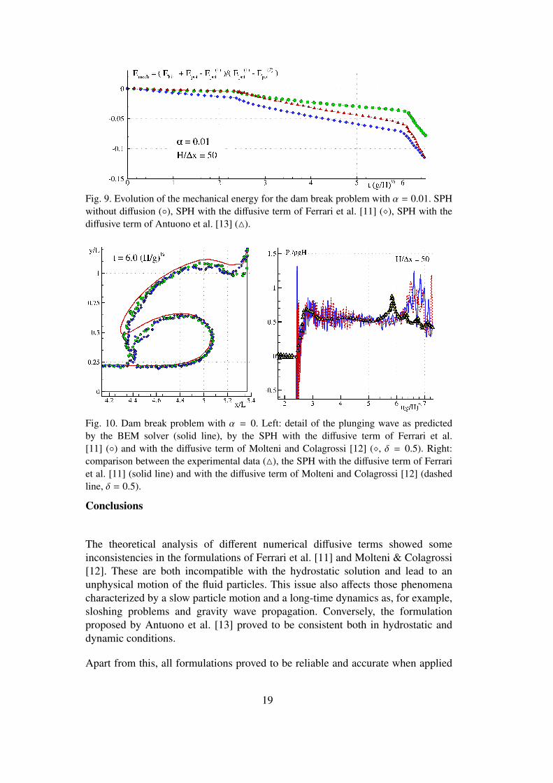
Fig. 9. Evolution of the mechanical energy for the dam break problem with α = 0.01. SPHwithout diffusion (), SPH with the diffusive term of Ferrari et al. [11] (), SPH with thediffusive term of Antuono et al. [13] (4).

Fig. 10. Dam break problem with α = 0. Left: detail of the plunging wave as predictedby the BEM solver (solid line), by the SPH with the diffusive term of Ferrari et al.[11] () and with the diffusive term of Molteni and Colagrossi [12] (, δ = 0.5). Right:comparison between the experimental data (4), the SPH with the diffusive term of Ferrariet al. [11] (solid line) and with the diffusive term of Molteni and Colagrossi [12] (dashedline, δ = 0.5).

Conclusions

The theoretical analysis of different numerical diffusive terms showed someinconsistencies in the formulations of Ferrari et al. [11] and Molteni & Colagrossi[12]. These are both incompatible with the hydrostatic solution and lead to anunphysical motion of the fluid particles. This issue also affects those phenomenacharacterized by a slow particle motion and a long-time dynamics as, for example,sloshing problems and gravity wave propagation. Conversely, the formulationproposed by Antuono et al. [13] proved to be consistent both in hydrostatic anddynamic conditions.

Apart from this, all formulations proved to be reliable and accurate when applied

19

to problems characterized by energetic events and short-time dynamics (as, forexample, water jets and impacts). In this context, the formulations of Ferrari etal. [11] and Molteni & Colagrossi [12] showed a stronger smoothing action on thepressure field than the formulation of Antuono et al. [13].

Acknowledgements

The Authors would like to thank Dr. Andrea Di Mascio and Prof. MaurizioBrocchini for their useful comments and suggestions. The research leading to theseresults has received funding from the European Community’s Seventh FrameworkProgramme (FP7/2007-2013) under grant agreement n. 225967 “NextMuSE” andby the Centre of Excellence for Ship and Ocean Structures of NTNU Trondheim(Norway) within the “Violent Water-Vessel Interactions and Related StructuralLoad”.

A Analysis of the diffusive terms

In this section we analyze the diffusive terms of Ferrari et al. [11] and of Antuonoet al. [13] at the continuum. In this context, we denote by r and r′ two pointsin the fluid domain and all the quantities evaluated at r′ are indicated throughthe superscript “prime” (i.e., f ′ indicates f (r′)). For the ease of the notation,we also use ∆ = r′ − r while the subscripts i, j, k, p denote the components ofvectors/tensors.

A.1 The diffusive term of Ferrari et al. [11]

Here we show the asymptotic behavior of the diffusive term proposed by Ferrari etal. [11] for h going to zero. Expanding (2.12) into a Taylor series, we find:

ΨFe =‖∆‖

2 h

[∂ρ

∂ri∆i +

12

∂2ρ

∂ri∂r j∆i ∆ j + O(‖∆‖3)

]. (A.1)

Using q = ∆/h, we get:

ΨFe = h‖q‖2

[∂ρ

∂riqi +

12

∂2ρ

∂ri∂r j∆i q j + O(‖∆‖2)

], (A.2)

which, substituted in (3.14), gives (3.15). The same procedure can be repeated forthe diffusive term proposed by Molteni & Colagrossi [12] leading to (2.9).

20

A.2 The diffusive term of Antuono et al. [13]

Let us consider a generic scalar field f (r). In analogy with the term ψi j defined in(2.10), we study the following function:

ΨAn =

(f ′ − f

)−

12

(∂ f ′

∂ri+∂ f∂ri

)∆i

. (A.3)

Then, using a Taylor expansion, we get:

f ′= f +∂ f∂ri

∆i +12

∂2 f∂ri∂r j

∆i ∆ j +16

∂3 f∂ri∂r j∂rk

∆i ∆ j ∆k +

+1

24∂4 f

∂ri∂r j∂rk∂rp∆i ∆ j ∆k ∆p + O(‖∆‖5) . (A.4)

In the same way, we obtain:

f= f ′ −∂ f ′

∂ri∆i +

12∂2 f ′

∂ri∂r j∆i ∆ j −

16

∂3 f ′

∂ri∂r j∂rk∆i ∆ j ∆k +

+1

24∂4 f ′

∂ri∂r j∂rk∂rp∆i ∆ j ∆k ∆p + O(‖∆‖5) (A.5)

that can be rearranged as follows:

f ′= f +∂ f ′

∂ri∆i −

12∂2 f ′

∂ri∂r j∆i ∆ j +

16

∂3 f ′

∂ri∂r j∂rk∆i ∆ j ∆k +

−1

24∂4 f ′

∂ri∂r j∂rk∂rp∆i ∆ j ∆k ∆p + O(‖∆‖5) . (A.6)

Now, summing (A.4) and (A.6) and rearranging, we find:

Ψ =14

[∂2 f∂ri∂r j

−∂2 f ′

∂ri∂r j

]∆i ∆ j +

112

[∂3 f

∂ri∂r j∂rk+

∂3 f ′

∂ri∂r j∂rk

]∆i ∆ j ∆k +

+1

48

[∂4 f

∂ri∂r j∂rk∂rp−

∂4 f ′

∂ri∂r j∂rk∂rp

]∆i ∆ j ∆k ∆p + O(‖∆‖5) . (A.7)

Then, using the following expansions:

∂2 f ′

∂ri∂r j=

∂2 f∂ri∂r j

+∂3 f

∂ri∂r j∂rk∆k +

12

∂4 f∂ri∂r j∂rk∂rp

∆k ∆p + O(‖∆‖3)

∂3 f ′

∂ri∂r j∂rk=

∂3 f∂ri∂r j∂rk

+∂4 f

∂ri∂r j∂rk∂rp∆p + O(‖∆‖2)

∂4 f ′

∂ri∂r j∂rk∂rp=

∂4 f∂ri∂r j∂rk∂rp

+ O(‖∆‖)

21

we, finally, get:

ΨAn = −112

∂3 f∂ri∂r j∂rk

∆i ∆ j ∆k −1

24∂4 f

∂ri∂r j∂rk∂rp∆i ∆ j ∆k ∆p + O(‖∆‖5) . (A.8)

Substituting (A.8) into (3.14) with f = ρ, we obtain the expansion for h going tozero of the diffusive term proposed by Antuono et al. [13]:

DAn =h6

(∂3ρ

∂ri∂r j∂rk

) ∫Ω

qi q j qk

q∂W∂q

dV ′ +

+h2

12

(∂4ρ

∂ri∂r j∂rk∂rp

) ∫Ω

qi q j qk qp

q∂W∂q

dV ′ + O(h3) (A.9)

where Ω is the fluid domain. Now, let us consider the following tensors:

Ai jk =

∫Ω

qi q j qk

q∂W∂q

dV ′ Bi jkp =

∫Ω

qi q j qk qp

q∂W∂q

dV ′ . (A.10)

If the point r is inside the fluid, the tensorA is identically zero because of symmetrywhile, on the contrary, the tensor B is generally non-zero. For this reason, thediffusive term is said to be a fourth-order differential operator. If the point r belongsto the free surface,A is no longer zero. In any case, the corresponding contributionis of order h and, therefore, the diffusive term always converges to zero for h goingto zero.

In one dimension and for a Gaussian kernel it is:

BGauss = −32

=⇒ DAn = −h2

8d4ρ

dx4 . (A.11)

In section 3.1 we compute the range of variability of the coefficient δ using a one-dimensional linear stability analysis. In this context, the diffusive term is indicatedby:

DAn = − h2 Bd4ρ

dx4 (A.12)

and the parameter B depends on the adopted kernel function (B = 1/8 for theGaussian kernel).

References

[1] S. Shao & Y.M.L. Edmond, Incompressible SPH method for simulating Newtonianand non-Newtonian flows with a free surface, Adv. Water Res. 26, 787–800, (2003)

[2] M. Ellero, M. Serrano, P. Español, Incompressible smoothed particle hydrodynamics,J. Comp. Phys., 226, 1731–1752, (2007).

22

[3] J.J. Monaghan, Simulating Free Surface Flows with SPH, J. Comp. Phys., 110, 399–406, (1994).

[4] J. Bonet & T.S.L. Lock, Variational and momentum preservation aspects of SmoothedParticle Hydrodynamics formulations, Comput. Methods Appl. Mech. Eng. 180, 97–115, (1999)

[5] A. Colagrossi, M. Antuono, D. Le Touzé, Theoretical considerations on the freesurface role in the SPH model, Physical Review E, 79/5, 056701: 1-13, (2009).

[6] J.J. Monaghan & R.A. Gingold, Shock Simulation by the Particle Method SPH, J.Comp. Phys., 52, 374–389, (1983).

[7] A. Colagrossi and M. Landrini, Numerical Simulation of Interfacial Flows bySmoothed Particle Hydrodynamics, Journal of Computational Physics, 191, 448–475,(2003).

[8] S. Sibilla, SPH simulation of local scour processes, Proc. SPHERIC, 2nd InternationalWorkshop, Universidad Politécnica de Madrid, Spain, May, (2007).

[9] J.P. Vila, On particle weighted methods and smooth particle hydrodynamics, Math.Models Methods Appl. Sci., 9/2, 161-209, (1999).

[10] B.B. Moussa and J.P. Vila, Convergence of SPH Method for scalar nonlinearconservation laws, SIAM J. Numer. Anal., 37/3, 863-887, (2000).

[11] A. Ferrari, M. Dumbser, E.F. Toro, A. Armanini, A new 3D parallel SPH scheme forfree-surface flows, Computers & Fluids, 38, 1203-1217, (2009).

[12] D. Molteni & A. Colagrossi, A simple procedure to improve the pressure evaluationin hydrodynamic context using the SPH, Computer Physics Communications, 180(6),861–872, (2009).

[13] M. Antuono, A. Colagrossi, S. Marrone, D. Molteni Free-surface flows solvedby means of SPH schemes with numerical diffusive terms, Computer PhysicsCommunications, 181, 532-549, (2010).

[14] J.J. Monaghan, Smoothed Particle Hydrodynamics, Rep. Prog. Phys. 68, 1703–1759,(2005).

[15] P.A. Madsen & H.A. Sh affer, A discussion of artificial compressibility, CoastalEngineering, 53, 93-98, (2006).

[16] M. Antuono, A. Colagrossi, S. Marrone, C. Lugni, Propagation of gravitywaves through a SPH schemes with numerical diffusive terms, Computer PhysicsCommunications, 182, 866-877, (2011).

[17] P.W. Randles & L.D. Libersky, Smoothed Particle Hydrodynamics: Some recentimprovements and applications Comput. Methods Appl. Mech. Engng., 139, 375-408,(1996).

[18] P. Español & M. Revenga, Smoothed dissipative particle dynamics, Physical ReviewE, 67, 026705 1–12, (2003).

23

[19] S. Gottlieb & C-W. Shu, Total variation diminishing Runge-Kutta schemes,Mathematics of Computation, 67(221), 73-85, (1998).

[20] A. Jamenson, W. Schmidth, E. Turkel, Numerical Solution of the Euler Equations byFinite Volume Methods Using Runge-Kutta Time-Stepping Schemes, AIAA 14-th Fluidand Plasma Dynamics Conference, Palo Alto, CA, June 23-25 (1981).

[21] J.J. Monaghan, A. Kos, Solitary waves on a Cretan beach, J. Waterway, Port, Coastaland Ocean Engng. 125, 145–154, (1999).

[22] J. P. Morris, P. J. Fox, Y. Zhu, Modeling Low Reynolds Number Incompressible FlowsUsing SPH, Journal of computational Physics, 136, 214-226, (1997).

[23] S. Marrone, M. Antuono, A. Colagrossi, G. Colicchio, D. Le Touzé, G. Graziani,δ-SPH model for simulating violent impact flows, Comput. Methods Appl. Mech.Engrg., 200, 1526-1542, (2011).

[24] M. Landrini, A. Colagrossi, M. Greco, M.P. Tulin, Gridless simulations of splashingprocesses and near-shore bore propagation, J. Fluid Mech. 591, 183-213, (2007).

[25] B. Buchner, Green Water on Ship-type Offshore Structures, Ph.D. Thesis, DelftUniversity of Technology, (2002).

[26] M. Greco, A Two-dimensional Study of Green-Water Loading PhD Thesis Universityof Trondheim, Norway, (2001).

24