LLNL-JRNL-416574

Maximum-Entropy Meshfree Method forCompressible and Near-IncompressibleElasticity

A. Ortiz, M. A. Puso, N. Sukumar

September 4, 2009

Computer Methods in Applied Mechanics and Engineering

Disclaimer

This document was prepared as an account of work sponsored by an agency of the United States government. Neither the United States government nor Lawrence Livermore National Security, LLC, nor any of their employees makes any warranty, expressed or implied, or assumes any legal liability or responsibility for the accuracy, completeness, or usefulness of any information, apparatus, product, or process disclosed, or represents that its use would not infringe privately owned rights. Reference herein to any specific commercial product, process, or service by trade name, trademark, manufacturer, or otherwise does not necessarily constitute or imply its endorsement, recommendation, or favoring by the United States government or Lawrence Livermore National Security, LLC. The views and opinions of authors expressed herein do not necessarily state or reflect those of the United States government or Lawrence Livermore National Security, LLC, and shall not be used for advertising or product endorsement purposes.

Maximum-Entropy Meshfree Method for Compressible

and Near-Incompressible Elasticity

A. Ortiza, M. A. Pusob, N. Sukumar∗,a

aDepartment of Civil and Environmental Engineering, University of California

One Shields Avenue, Davis, CA 95616, U.S.A.bLawrence Livermore National Laboratory, P.O. Box 808, Livermore, CA 94551, U.S.A.

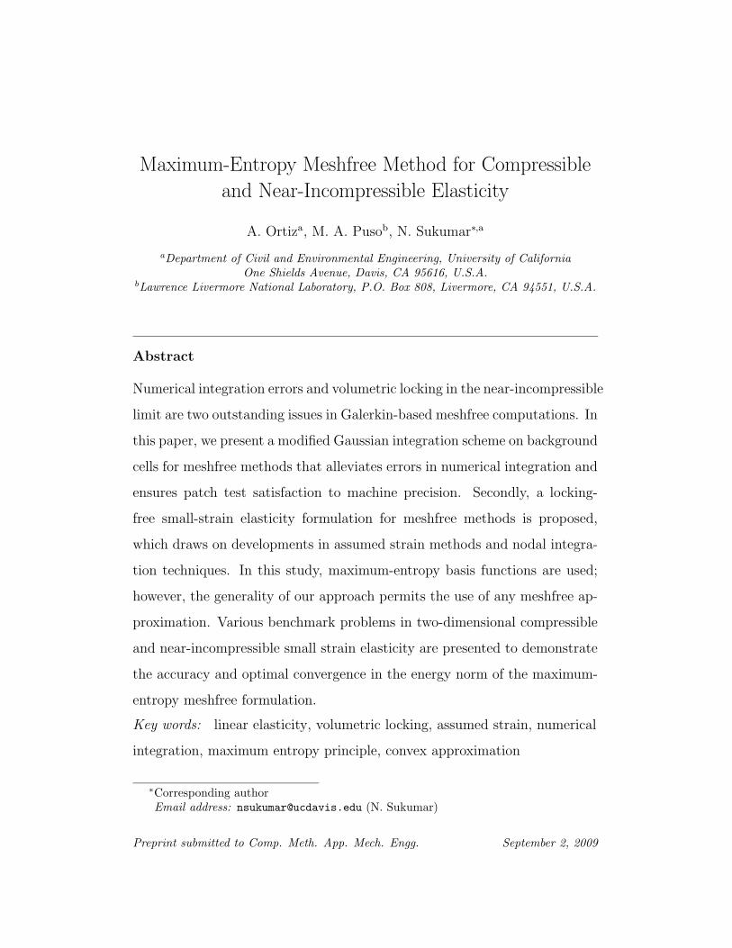
Abstract

Numerical integration errors and volumetric locking in the near-incompressible

limit are two outstanding issues in Galerkin-based meshfree computations. In

this paper, we present a modified Gaussian integration scheme on background

cells for meshfree methods that alleviates errors in numerical integration and

ensures patch test satisfaction to machine precision. Secondly, a locking-

free small-strain elasticity formulation for meshfree methods is proposed,

which draws on developments in assumed strain methods and nodal integra-

tion techniques. In this study, maximum-entropy basis functions are used;

however, the generality of our approach permits the use of any meshfree ap-

proximation. Various benchmark problems in two-dimensional compressible

and near-incompressible small strain elasticity are presented to demonstrate

the accuracy and optimal convergence in the energy norm of the maximum-

entropy meshfree formulation.

Key words: linear elasticity, volumetric locking, assumed strain, numerical

integration, maximum entropy principle, convex approximation

∗Corresponding authorEmail address: nsukumar@ucdavis.edu (N. Sukumar)

Preprint submitted to Comp. Meth. App. Mech. Engg. September 2, 2009

1. Introduction

It is well-known that standard displacement-based Galerkin formulations

exhibit severe stiffening when modeling near-incompressible materials. In

elasticity theory, this occurs when the Poisson’s ratio ν approaches 1/2, and

is referred to as volumetric locking. In finite elements, some of the approaches

to alleviate locking are: reduced/selective integration [1], B-bar technique [2],

mixed formulations [3], and assumed strain methods [4]. Displacement-based

Galerkin meshfree methods [5, 6, 7, 8, 9, 10, 11, 12, 13] that are based on

moving least squares approximants, natural neighbor interpolants, or entropy

approximants are also prone to locking. Huerta and Fernandez-Mendez [14]

have conducted an indepth study of volumetric locking in the element-free

Galerkin (EFG) method. Various remedies have been pursued in the litera-

ture to overcome this deficiency—for instance, Dolbow and Belytschko [15]

employed reduced integration techniques within a mixed formulation of the

EFG method; Gonzalez et al. [16] enriched the displacement approxima-

tion in a mixed natural element formulation; Vidal et al. [17] used pseudo-

divergence-free approximants in the EFG to satisfy the incompressibility con-

dition; and the B-bar and enhanced strain methods were introduced in the

EFG by Recio et al. [18]. In an effort to depart from background cell in-

tegration, stabilized nodal integration [19, 20, 21, 22, 23] and stress-point

integration schemes [24, 25, 26] have also been proposed to overcome nu-

merical integration errors and facilitate large deformation simulations with

meshfree methods. These approaches attempt to mimic reduced integration

2

procedures, and have had success in suppressing volumetric locking.

Traditionally, numerical integration of the weak form in meshfree meth-

ods is carried out using background cells—triangular or quadrilateral ele-

ments are typically adopted in two dimensions [6]. Meshfree basis functions

are non-polynomial and in addition the support of the basis functions no

longer coincides with the union of the background cells that are used in the

numerical integration. This leads to inaccuracies in the numerical integration

of weak form integrals, and patch test is not passed to machine precision.

In the EFG method, Belytschko et al. [6] used higher-order Gauss quadra-

ture in each background cell, and in a subsequent study by Dolbow and

Belytschko [27], integration cells that were aligned with the support of the

nodal basis functions were used. Griebel and Schweitzer [28] developed a

partition of unity meshfree method by formulating a hierarchical algorithm

to construct a nodal cover by partitioning the domain into overlapping hyper-

rectangular patches using d-dimensional trees. Due to the overlapping nodal

patches, a decomposition of the patches into disjoint cells was performed,

and these cells were used as the integration domains. A sparse grid quadra-

ture rule based on univariate Gauss-Patterson rules was employed [29]. As

a departure from covers that are rectangular, Riker and Holzer [30] recently

proposed a partition-of-unity method in which the nodal cover is a combina-

tion of simplexes and polygons.

Atluri et al. [31] proposed a methodology to integrate the weak form in

the meshless local Petrov-Galerkin method without the need for background

cells by using the support of the basis functions as the domain of integra-

tion. This approach was adopted and improved upon in the work of De and

3

Bathe [32]. Similar ideas have also been pursued in Refs. [33, 34, 35, 36].

With the aim of using anisotropic weight functions with reduced support

sizes, Balachandran et al. [37] developed a methodology that automatically

confines the basis functions to natural neighbor polygonal regions by means

of the Schwarz-Christoffel mapping. The resulting basis functions are used

within a MLS-based meshfree method. Liu and Tu [38] developed an adap-

tive procedure within individual background cells for meshfree methods. One

of the first theoretical studies on the influence of numerical quadrature errors

in meshfree methods was recently put forth by Babuska et al. [39]. Schem-

bri et al. [40] compare the performance of different meshfree approximation

schemes in three-dimensional computations.

In the past few years, there has been renewed efforts to remedy the poor

performance of low-order triangular and tetrahedral finite elements in the

near-incompressible regime [41, 42, 43, 44, 45, 46, 47, 48]. These approaches

are broadly based on the idea of reducing the number of incompressibility

constraints by defining nodal-averaged pressures or strains. In Ref. [48],

a special form of a nodal strain matrix was computed from the elements

attached to the node, and it led to a locking-free displacement-based formu-

lation. Although these nodal methods tend not to lock, several authors have

reported pressure oscillations for highly constrained problems [45, 46].

In this paper, we present new techniques for meshfree methods that pro-

vide patch test accuracy in cell-based numerical integration, and a remedy

for volumetric locking in the incompressible limit. Our approach for the lat-

ter uses the notion of nodal-averaged pressure and leads to a displacement-

formulation as in Krysl and Zhu [48]; however, we differ in that the starting

4

point of our method is the displacement/pressure mixed formulation, and

numerical integration is tailored for meshfree basis functions using Gauss

quadrature. Since numerical errors are prevalent when standard tensor-

product Gauss quadrature is used in meshfree methods, we appeal to as-

sumed strain methods [49] and nodal integration techniques [20, 21, 22] to

define a modified strain tensor. Maximum-entropy basis functions [13, 50] are

used to define the modified strain matrix, and Gauss quadrature is adopted

in the numerical integration. The procedure so devised alleviates numerical

integration errors in meshfree methods using minimal number of integration

points and ensures patch test satisfaction to within machine precision.

One of the basic motivations for using meshfree basis functions is they

tend to be much more insensitive to poor discretizations and large defor-

mation mesh distortions. Although, automatic mesh generation technology

is very mature, there are still instances, particularly in three dimensions,

where these mesh generators produce poor tesselations such that near slivers

occur. Standard Lagrange shape functions break down in these instances1,

but meshfree basis functions typically do not. The distortion insensitivity

of meshfree methods using integration cells also makes them more robust in

large deformations settings. Lagrange elements have a tendency to invert in

many tough problems and as such, commercial codes such as LS-DYNATM

offer a meshfree element as an alternative.

The remainder of this paper is structured as follows: In Section 2, a brief

introduction to maximum-entropy basis functions is presented. In Section 3,

1The element Jacobian, computed from shape function derivatives, becomes singular.

5

the new formulation for compressible and near-incompressible material be-

havior is developed. In Section 4, the improved numerical integration scheme

is elaborated for two-dimensional background meshes. Numerical examples

are presented in Section 5 for benchmark problems in compressible and near-

incompressible media to demonstrate the improved numerical integration and

the amelioration of volumetric locking. Finally, we close with some final re-

marks in Section 6.

2. Maximum-entropy basis functions

On using the Shannon entropy [51], Jaynes postulated the principle of

maximum entropy [52] as a rationale means for least-biased statistical infer-

ence when insufficient information is available. The principle of maximum

entropy is suitable to find the least-biased probability distribution when there

are fewer constraints than unknowns (incomplete information). In the con-

text of meshfree approximants, the probability distribution corresponds to

the set of basis functions associated with scattered set of nodes at locations

xana=1. Thus, basis functions are viewed as the probability of influence of

the nodes at any point x that lies in the convex hull of the set x1,x2, . . . ,xn.

The connection between maximum entropy (max-ent) basis functions

and linearly complete approximations was established by Sukumar [53]. In

Ref. [53], the principle of maximum entropy was employed to obtain lin-

ear approximants on polygonal domains. Arroyo and Ortiz [13] realized a

meshfree approximation using a modified entropy functional—with empha-

sis on establishing a smooth transition between meshfree and finite element

methods. Sukumar and Wright [50] generalized the construction of max-

6

ent meshfree basis functions by using the relative (Shannon-Jaynes) entropy

functional with a prior [54]. On using compactly-supported prior weight

functions that are at least C0, compactly-supported max-ent basis functions

are realized. In particular, when a Gaussian prior is employed the approach

of Arroyo and Ortiz [13] is recast. Maximum-entropy basis functions are

obtained from a convex optimization problem and are endowed with the fol-

lowing attributes [13]: variation diminishing property; positive-definite mass

matrices and weak Kronecker-delta property on the boundary. The last prop-

erty is noteworthy since it enables the direct imposition of essential boundary

conditions as in finite elements. Recall that most meshfree methods need

to resort to special technique to enforce essential boundary conditions (for

example, see Refs. [55, 56, 57]). Recently, new applications of max-ent mesh-

free basis functions have emerged: co-rotational formulation is presented in

Ref. [58] and second-order max-ent approximants are proposed in Ref. [59].

We now follow the approach of Ref. [50] to present expressions for max-ent

basis functions and their derivatives. To this end, let the prior weight function

be denoted by wa(x). The set of max-ent basis functions φa(x) ≥ 0na=1 is

obtained via the solution of the following optimization problem:

maxφ∈Rn

+

−n∑

a=1

φa(x) ln

(

φa(x)

wa(x)

)

, (1a)

subject to the linear reproducing conditions:

n∑

a=1

φa(x) = 1,n∑

a=1

φa(x)xa = 0, (1b)

where we have made use of shifted nodal coordinates xa = xa−x. Applying

the procedure of Lagrange multipliers, the following expression for max-ent

7

basis functions is obtained:

φa(x) =Za(x;λ)

Z(x;λ), Za(x;λ) = wa(x) exp(−λ · xa), (2)

where Z(x;λ) =∑

b Zb(x;λ), and in two dimensions xa = [xa ya]T and

λ = [λ1 λ2]T. In Eq. (2), the Lagrange multiplier vector λ is determined

from the dual of the optimization problem posed in Eq. (1)—λ is found

by minimizing lnZ, which gives rise to the following system of nonlinear

equations:

f(λ) = ∇λ lnZ(λ) = −n∑

a

φa(x)xa = 0, (3)

where ∇λ stands for the gradient with respect to λ. Examples of prior

weight functions include Gaussian radial basis functions [13] and quartic

polynomials [58]:

wa(x) = exp(−βa‖xa − x‖2), (4a)

wa(q) =

1− 6q2 + 8q3 − 3q4, 0 ≤ q ≤ 1

0, q > 1, (4b)

where βa = γ/h2a; γ is a parameter that controls the support-width of the

basis function at node a; and ha is a characteristic nodal spacing that may be

distinct for each node a. In two dimensions, we set ha as the second-nearest

nodal distance to node a. For the quartic polynomial, q = ‖xa − x‖/ρa

and ρa = γha is the radius of the basis function support at node a. In the

optimization problem, once the converged λ is obtained, the basis functions

are computed from Eq. (2) and the gradient of the basis function is [58]:

∇φa = φa

[

xa ·(

H−1 −H−1 ·A)

+∇wa

wa

−n∑

b=1

φb

∇wb

wb

]

, (5a)

8

where

A =n∑

b=1

φbxb ⊗∇wb

wb

(5b)

and H is the Hessian matrix

H = ∇λf = ∇λ∇λ lnZ =n∑

b=1

φbxb ⊗ xb. (5c)

In Fig. 1, plots of a max-ent basis function and its derivatives for a quar-

tic prior function are illustrated. For the Gaussian prior weight function,

Eq. (5a) reduces to [13]

∇φa = φaH−1 · xa. (6)

3. Governing equations and mixed formulation

3.1. Strong form

Consider a body defined by an open bounded domain Ω ⊂ R2 with bound-

ary Γ such that Γ = Γu∪Γt and Γu∩Γt = ∅. Linear isotropic elasticity under

static loads and no body force with validity for both compressible and near-

incompressible material behavior is governed by the following equations [1]:

∇ · σ = 0 in Ω, (7a)

∇ · u+p

λ= 0 in Ω, (7b)

together with the following essential (displacement) and natural (traction)

boundary conditions imposed on Γu and Γt, respectively:

u = u on Γu, (7c)

σ · n = t on Γt, (7d)

9

(a) (b)

(c) (d)

Fig. 1: Plots of quartic prior weight function and maximum-entropy basis function and

its derivatives for node a. Note that wa(xa) = 1, but φa(xa) 6= 1, and hence the interior

basis function φa does not satisfy the Kronecker-delta property. (a) Quartic prior, wa; (b)

φa; (c) ∂φa/∂x; and (d) ∂φa/∂y.

10

where the Cauchy stress tensor σ is related to the small strain tensor ε and

the pressure parameter p by the following isotropic linear elastic constitutive

relation:

σ(u, p) = −pI+ 2µε(u). (7e)

In Eq. (7), λ and µ are Lame parameters which for plane strain are defined

as

λ =νE

(1 + ν)(1− 2ν), µ =

E

2(1 + ν), (8)

where ν is the Poisson’s ratio and E is the Young’s modulus of the material.

The kinematic relation between the small strain tensor ε and the displace-

ment vector u is

ε =1

2[u⊗∇ + ∇⊗ u] . (9)

3.2. Weak form

Consider trial functions ui(x) ∈ H1(Ω) and test functions δui(x) ∈ H10(Ω)

(i = 1, 2), where H1(Ω) is the Sobolev space of functions with square-

integrable first derivatives in Ω, and H10(Ω) is the Sobolev space of func-

tions with square-integrable first derivatives in Ω and vanishing values on

the essential boundary Γu. Also, the trial function for the pressure param-

eter p ∈ H0(Ω) and test functions δp ∈ H0(Ω), where H0(Ω) ≡ L2(Ω) is

the Sobolev space of square-integrable functions. The weak form (principle

virtual work) for the displacement/pressure mixed formulation is [1]:

∫

Ω

δεijσij dΩ−

∫

Γt

δuiti dΓ = 0 ∀δui ∈ H10(Ω), (10a)

∫

Ω

δp(

εkk +p

λ

)

dΩ = 0 ∀δp ∈ H0(Ω). (10b)

11

3.3. Discrete weak form

In the standard displacement/pressure mixed formulation, the discretiza-

tion procedure of the weak form yields a system of linear equations where

both displacement and pressure parameter are part of the unknown vector.

Our approach is distinct: starting from the weak form given in Eq. (10), we

construct a displacement-based weak form such that the pressure approxi-

mation is obtained a posteriori from the displacement field. To this end,

let us discretize the pressure parameter p using linear finite element shape

functions over a two-dimensional mesh of triangles:

ph(x) =3∑

a=1

Na(x)pa, (11)

where pa are nodal pressures2. The displacement is discretized using maximum-

entropy basis functions:

uh(x) =N∑

a=1

φa(x)ua, (12)

which yields the following expression for the volumetric strain:

εhkk(x) =

[

1 1 0]

N∑

a=1

Ba(x)ua = mT

N∑

a=1

Ba(x)ua, (13)

where ua are nodal displacement coefficients and Ba(x) is the strain matrix

for node a:

Ba(x) =

φa,x 0

0 φa,y

φa,y φa,x

. (14)

2Although meshfree shape functions could potentially be used here, finite element shape

functions are used for simplicity. Since no shape function derivatives of this field is re-

quired, poor tesselations or large distortions is not likely to drastically affect results.

12

In order to ensure stability of the solution [1], the displacement approxi-

mation is enhanced with an extra displacement node in the interior of each

triangle. This approach bears resemblance to the use of nodal bubble shape

functions in finite element methods [60], even though in the present case the

max-ent basis function of the interior node does not necessarily vanish on

the boundary of the triangle. See Ref. [61] for a related study on meshfree

methods involving bubble functions. On substituting Eqs. (11) and (13) into

Eq. (10), and relying on the arbitrariness of nodal pressure variations yields

N∑

b=1

∫

Ω

NamTBbub dΩ +

1

λ

3∑

b=1

∫

Ω

NaNbpb dΩ = 0, (15)

and performing row-sum in the pressure term leads to

N∑

b=1

∫

Ω

NamTBb dΩ

ub +

1

λ

∫

Ω

Na dΩ

pa = 0. (16)

From Eq. (16), we obtain the nodal pressure as

pa = −λN∑

b=1

∫

ΩNam

TBb dΩ∫

ΩNa dΩ

ub, (17)

which we refer to as volume-averaged nodal pressure. For the purpose of com-

putation of integrals in Eq. (17), Ω is the union of all the elements attached

to node a, i.e., Ω = ∪Ωea.

Even though our approach shares common features with the method pro-

posed by Krysl and Zhu [48], there exist notable differences. We use aver-

ages of strain matrices from the elements attached to a particular node to

satisfy the near-incompressibility constraint in the weak form (10), whereas

in Ref. [48] the averages are used to obtain a strain field that satisfies a

13

a

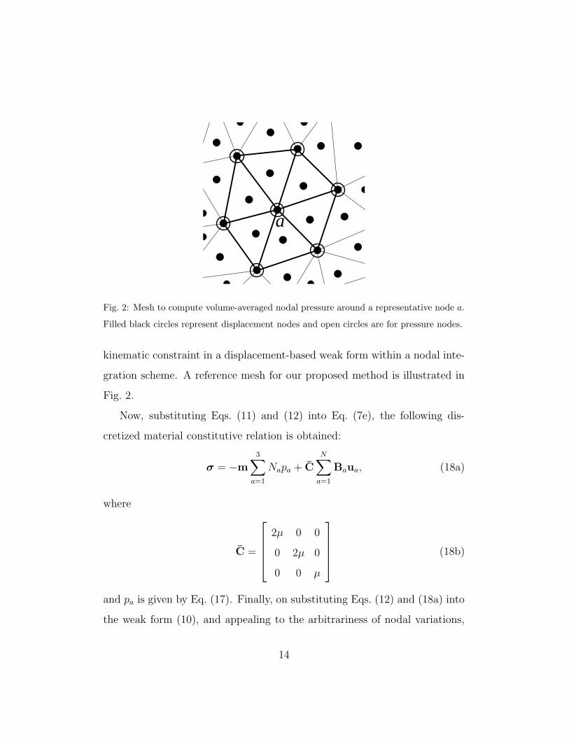
Fig. 2: Mesh to compute volume-averaged nodal pressure around a representative node a.

Filled black circles represent displacement nodes and open circles are for pressure nodes.

kinematic constraint in a displacement-based weak form within a nodal inte-

gration scheme. A reference mesh for our proposed method is illustrated in

Fig. 2.

Now, substituting Eqs. (11) and (12) into Eq. (7e), the following dis-

cretized material constitutive relation is obtained:

σ = −m3∑

a=1

Napa + C

N∑

a=1

Baua, (18a)

where

C =

2µ 0 0

0 2µ 0

0 0 µ

(18b)

and pa is given by Eq. (17). Finally, on substituting Eqs. (12) and (18a) into

the weak form (10), and appealing to the arbitrariness of nodal variations,

14

the following discrete system of equations is obtained:

Kd = f , (19a)

where d is the vector of nodal coefficients and

Kab =

∫

Ω

BTa CBb dΩ−

∫

Ω

BTam

3∑

c=1

NcQcb

dΩ, (19b)

fa =

∫

Γt

φat dΓ, (19c)

with

Qcb = −λN∑

b=1

∫

ΩNcm

TBb dΩ∫

ΩNc dΩ

. (19d)

Note that owing to Eq. (17) in conjunction with Eq. (18), Eq. (19) depends

only on the displacement field. The pressure field p can be obtained a pos-

teriori from the displacement field through Eq. (17).

4. Modified Gauss integration

As in finite element methods, numerical integration is used in meshfree

methods to evaluate the weak form integrals that appear in Eq. (19). Typ-

ically, the support of meshfree basis functions is greater than the support

of finite element basis functions, which provides meshfree methods greater

flexibility and often leads to improved accuracy. However, this has its con-

sequences: with polynomial finite element basis functions whose support

includes the union of triangles in a two-dimensional Delaunay tesselation,

appropriate Gauss quadrature rules can be selected to ensure accurate and

optimally convergent finite element solutions. In meshfree methods, these

15

properties are lost, and hence use of standard Gauss quadrature to evaluate

Eq. (19) leads to errors in numerical integration. To overcome this deficiency

in existing meshfree methods, we devise a numerical integration scheme that

alleviates the aforementioned errors.

4.1. Assumed-strain method

We present a suitable modification to the standard Gauss quadrature to

remove integration errors in meshfree methods and ensure patch test satis-

faction to within machine precision. On appealing to assumed strain meth-

ods [49], we first perform the following modification to the weak form in

Eq. (10):∫

Ω

δεijσij dΩ−

∫

Γt

δuiti dΓ = 0 ∀δui ∈ H10(Ω), (20a)

∫

Ω

δp(

εkk +p

λ

)

dΩ = 0 ∀δp ∈ H0(Ω). (20b)

where now ε is an assumed strain which we refer to as the modified strain.

Now, let us consider the following modified strain in a certain background

finite element cell:

ε = ε− ε+ ¯ε, (21)

where ε is the standard small strain tensor, ε is the volume average strain

tensor over the background cell, and ¯ε corresponds to ε written as a surface

integral by means of Green’s theorem. The corresponding equations are

ε =1

2[u⊗∇ + ∇⊗ u] , (22a)

ε =1

V e

∫

Ωe

ε dΩ, (22b)

¯ε =1

V e

∫

Γe

1

2[u⊗ n+ n⊗ u] dΓ. (22c)

16

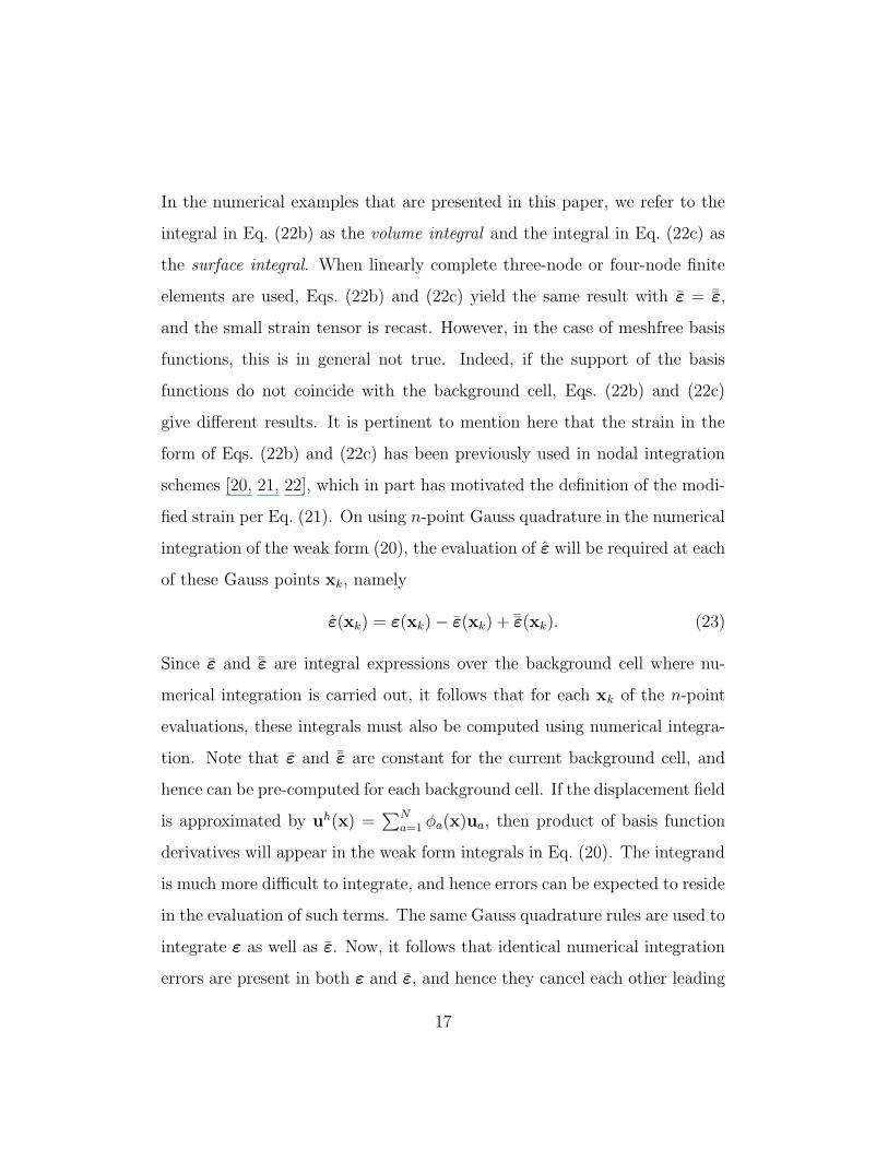
In the numerical examples that are presented in this paper, we refer to the

integral in Eq. (22b) as the volume integral and the integral in Eq. (22c) as

the surface integral. When linearly complete three-node or four-node finite

elements are used, Eqs. (22b) and (22c) yield the same result with ε = ¯ε,

and the small strain tensor is recast. However, in the case of meshfree basis

functions, this is in general not true. Indeed, if the support of the basis

functions do not coincide with the background cell, Eqs. (22b) and (22c)

give different results. It is pertinent to mention here that the strain in the

form of Eqs. (22b) and (22c) has been previously used in nodal integration

schemes [20, 21, 22], which in part has motivated the definition of the modi-

fied strain per Eq. (21). On using n-point Gauss quadrature in the numerical

integration of the weak form (20), the evaluation of ε will be required at each

of these Gauss points xk, namely

ε(xk) = ε(xk)− ε(xk) + ¯ε(xk). (23)

Since ε and ¯ε are integral expressions over the background cell where nu-

merical integration is carried out, it follows that for each xk of the n-point

evaluations, these integrals must also be computed using numerical integra-

tion. Note that ε and ¯ε are constant for the current background cell, and

hence can be pre-computed for each background cell. If the displacement field

is approximated by uh(x) =∑N

a=1 φa(x)ua, then product of basis function

derivatives will appear in the weak form integrals in Eq. (20). The integrand

is much more difficult to integrate, and hence errors can be expected to reside

in the evaluation of such terms. The same Gauss quadrature rules are used to

integrate ε as well as ε. Now, it follows that identical numerical integration

errors are present in both ε and ε, and hence they cancel each other leading

17

to accurate integration over the background cell. It is also worth noting that

the proposed modified strain will exactly satisfy the patch test; the proof is

provided in Appendix A.

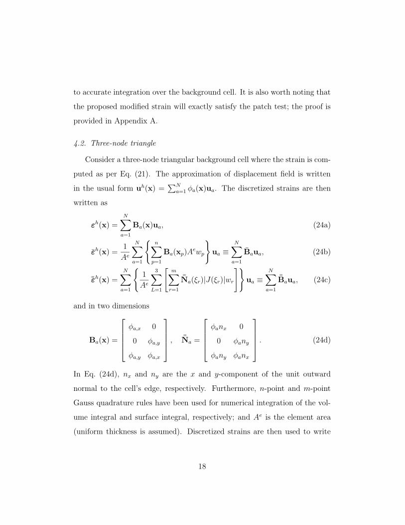
4.2. Three-node triangle

Consider a three-node triangular background cell where the strain is com-

puted as per Eq. (21). The approximation of displacement field is written

in the usual form uh(x) =∑N

a=1 φa(x)ua. The discretized strains are then

written as

εh(x) =N∑

a=1

Ba(x)ua, (24a)

εh(x) =1

Ae

N∑

a=1

n∑

p=1

Ba(xp)Aewp

ua ≡N∑

a=1

Baua, (24b)

¯εh(x) =N∑

a=1

1

Ae

3∑

L=1

[

m∑

r=1

¯Na(ξr)|J(ξr)|wr

]

ua ≡N∑

a=1

¯Baua, (24c)

and in two dimensions

Ba(x) =

φa,x 0

0 φa,y

φa,y φa,x

, ¯Na =

φanx 0

0 φany

φany φanx

. (24d)

In Eq. (24d), nx and ny are the x and y-component of the unit outward

normal to the cell’s edge, respectively. Furthermore, n-point and m-point

Gauss quadrature rules have been used for numerical integration of the vol-

ume integral and surface integral, respectively; and Ae is the element area

(uniform thickness is assumed). Discretized strains are then used to write

18

the discretized modified strain tensor as follows:

εh(x) =N∑

a=1

Ba(x)ua, (25a)

with

Ba(x) = Ba(x)−Ga, (25b)

and

Ga =n∑

p=1

Ba(xp)wp −1

Ae

3∑

L=1

m∑

r=1

¯Na(ξr)|J(ξr)|wr

. (25c)

4.3. Numerical integration of the stiffness matrix and external force vector

In Eq. (19), matrix Kab and vector fa are numerically integrated using n-

point Gauss quadrature rule. Recall that the same Gauss quadrature rule is

used in Eq. (22b). In particular, for a three-node triangular background cell,

the numerical integration of the stiffness matrix disregarding the pressure

part is computed as follows:

Kab =n∑

k=1

BTa (xk)CBb(xk)A

etwk, (26)

where Ae is the area of the three-node triangle and t its thickness. In Eq. (26),

indices a and b ranges over the nodes covered by the intersection of the

support of the basis functions contained in Ba and Bb.

5. Numerical examples

We study the accuracy and performance of the maximum-entropy mesh-

free (MEM) method by means of four two-dimensional benchmark problems:

19

displacement patch test, cantilever beam subjected to a parabolic end load,

Cook’s membrane problem, and rigid flat punch under frictionless indenta-

tion. For the cantilever beam and Cook’s membrane problems, we compare

the maximum-entropy solution to a finite element solution (MINI element).

In the numerical examples, we use the acronyms STD to refer to standard

Gaussian integration and MOD for modified Gaussian integration (see Sec-

tion 4). Unless stated otherwise, we use MOD with 3-point Gauss quadrature

for the volume integral and 2-point Gauss quadrature for the surface inte-

gral in the MEM computations. It is reminded that the implementation uses

only three stress points per triangle; the surface Gauss points only sample

displacement and are used to modify the strain at these stress points.

5.1. Displacement patch test

Consider the boundary-value problem for a two-dimensional elastic plate

under essential boundary conditions:

∇ · σ = 0 in Ω = (0, 1)2,

u1(x) = x1 on ∂Ω, u2(x) = x1 + x2 on ∂Ω.

Plane strain conditions are assumed with the following material parame-

ters: E = 3 × 107 and ν = 0.3; 0.499. The meshes used in the study are

shown in Fig. 3: a uniform mesh of four-node quadrilateral elements (Q4)

for ν = 0.3, and a non-uniform mesh of three-node triangular elements (T3)

for ν = 0.3; 0.499. Both meshes are tested using STD and MOD schemes.

Maximum-entropy basis functions are used with a support-width parameter

γ = 2.0 for the Gaussian prior, and γ = 1.5 for the quartic prior. Numerical

results for the relative error in the L2-norm are shown in Tables 1 and 2.

20

(a) (b)

Fig. 3: Meshes used for the displacement patch test. (a) Uniform mesh of four-node

quadrilaterals (Q4); and (b) Non-uniform mesh of three-node triangles (T3).

Different Gauss quadrature rules for the volume integrals are tested (quadra-

ture rule for quadrilateral elements is indicated within braces). Numerical

results confirm that patch test satisfaction is met to within machine precision

for both compressible and near-incompressible material behavior only when

MOD is employed. In this study, max-ent approximants are used, but the

generality of the integration approach renders it applicable to other meshfree

approximants as well as polygonal finite element interpolants [62].

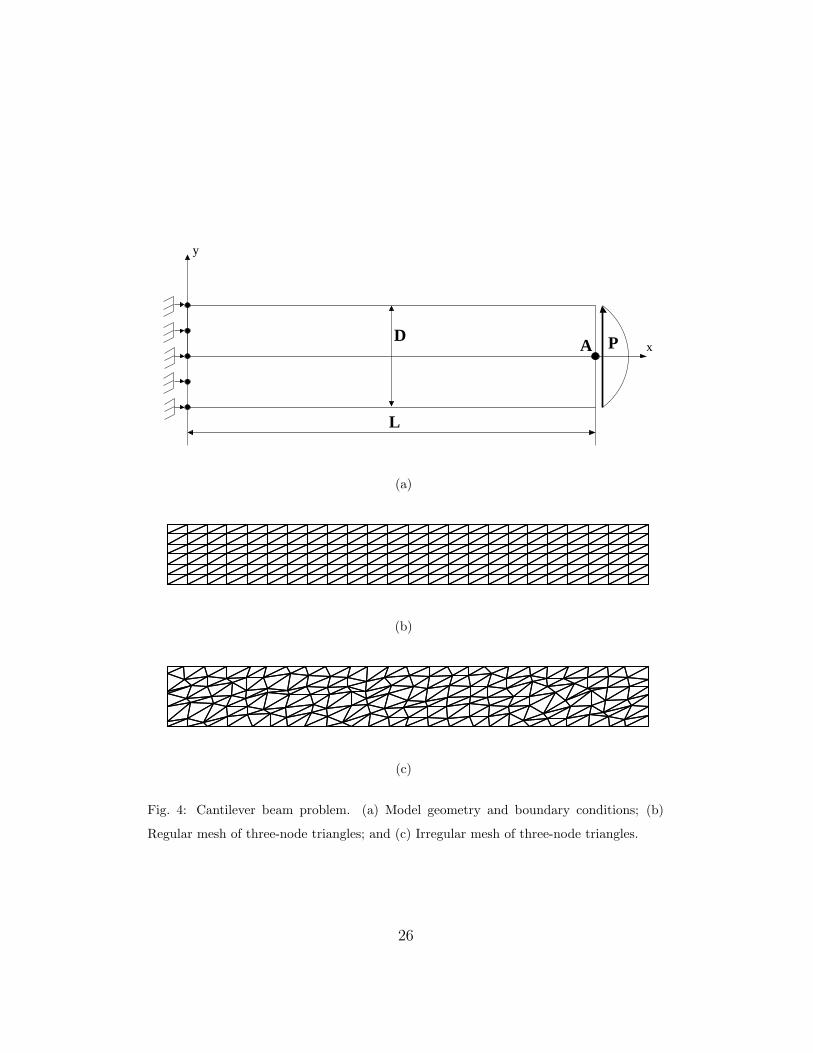
5.2. Cantilever beam

We consider the cantilever beam of thickness t with a a parabolic end

load P (Fig. 4(a)). The displacement solution for compressible (ν = 0.3) and

near-incompressible (ν = 0.499999) material behavior with E = 107 in plane

21

Table 1: Relative error in the L2-norm for the patch test (ν = 0.3)

Prior Quadrature T3 (STD) T3 (MOD) Q4 (STD) Q4 (MOD)

Gaussian

3 (3× 3) 1.7× 10−3 3.2× 10−16 6.4× 10−6 1.2× 10−15

6 (6× 6) 5.6× 10−4 3.1× 10−16 1.9× 10−8 2.8× 10−15

12 (12× 12) 2.9× 10−4 3.4× 10−16 6.6× 10−12 2.5× 10−15

Quartic

3 (3× 3) 2.6× 10−3 2.8× 10−16 1.3× 10−4 3.2× 10−16

6 (6× 6) 3.0× 10−3 4.4× 10−16 5.6× 10−7 9.3× 10−16

12 (12× 12) 7.8× 10−4 3.6× 10−16 1.3× 10−8 7.9× 10−16

Table 2: Relative error in the L2-norm for the patch test (ν = 0.499)

Prior Quadrature T3 (STD) T3 (MOD)

Gaussian

3 5.4× 10−1 8.2× 10−14

6 4.8× 10−1 8.8× 10−14

12 4.5× 10−1 8.6× 10−14

Quartic

3 5.2× 10−1 2.6× 10−13

6 3.9× 10−1 2.6× 10−13

12 5.1× 10−1 6.2× 10−13

22

strain condition is sought. Essential boundary conditions on the clamped

edge are applied according to the analytical solution given by Timoshenko

and Goodier [63]:

ux =Py

6EI

(

3x2 − 6Lx+ νy2)

−Py

6Iµ

(

y2 −3

4D2

)

, (28a)

uy =P

6EI

(

3ν (L− x) y2 + 3Lx2 − x3)

, (28b)

where µ is the material shear modulus (Lame parameter) and

E =

E for plane stress

E/ (1− ν2) for plane strain, (29a)

ν =

ν for plane stress

ν/ (1− ν) for plane strain. (29b)

In the numerical computations the following parameters are used: L = 16,

D = 4, t = 1 and P = −1. Two background meshes for the upper half of the

beam are studied: a regular mesh of three-node triangles (Fig. 4(b)) and an

irregular mesh of three-node triangles (Fig. 4(c)). Maximum-entropy basis

functions are used with a support-width parameter γ = 2.0 for the Gaussian

prior. The numerical solution of the maximum-entropy meshfree method

with MOD is compared to the finite element solution (MINI element [64]) for

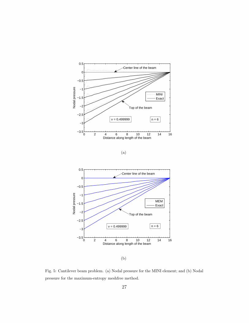
the standard displacement/pressure mixed formulation. Results for the nor-

malized tip deflection are shown in Table 3 for both meshes. The numerical

and exact solution for the nodal hydrostatic pressure along the fibers of the

beam (regular mesh only) are depicted in Fig. 5(a) for the MINI element and

in Fig. 5(b) for the maximum-entropy meshfree method. For the pressure

field, the MINI element has some oscillations about the analytical solution,

23

whereas the maximum-entropy solution is devoid of oscillations and is in very

good agreement with the analytical solution. The convergence study of the

normalized tip deflection for the regular mesh is shown in Fig. 6 for the MINI

element and the MEM method. The numerical results indicate that com-

pared to the finite element solution, the MEM solution has better accuracy

and converges faster towards the exact tip-deflection.

To assess the influence of numerical integration, a study of the MEM

method with STD and MOD schemes is conducted. The numerical results

for ν = 0.3 and ν = 0.499999 are presented in Fig. 7. For ν = 0.3, the

standard displacement-based max-ent formulation is used with nodes lo-

cated only at the vertices of the triangles. From the convergence curves

in Fig. 7(a), we observe that the rate of convergence of STD (with 3-, 6-, and

12-point quadrature) and MOD techniques are in agreement with theory.

For ν = 0.499999, the nodal-averaged pressure formulation is adopted, and

an additional displacement-node is inserted in the middle of every triangle.

It is evident from the curves in Fig. 7(b) that 3-point Gauss quadrature is

insufficient (under-integration leads to lack of convergence), and only with

higher-order Gauss quadrature is the convergence rate closer to optimal. This

is not surprising, since 3-point and 6-point quadrature in a triangle are ex-

act for second-order and fourth-order bivariate polynomials, respectively, but

the max-ent basis function for the interior node bears similarity to a cubic

bubble function, which renders the integrand of the stiffness matrix to be

like a fourth-order bivariate polynomial. Hence, the improved accuracy with

6-point quadrature is realized, with 12-point quadrature being able to deliver

about the same accuracy as the modified integration scheme. The numerical

24

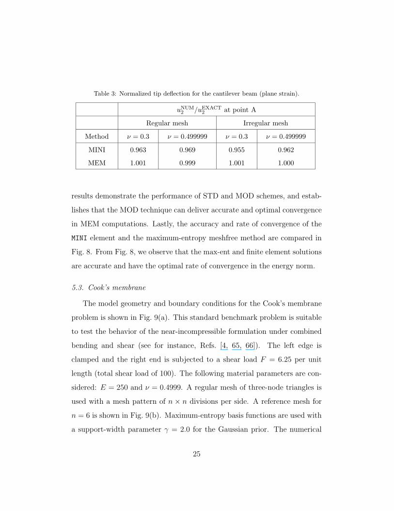
Table 3: Normalized tip deflection for the cantilever beam (plane strain).

uNUM2 /uEXACT2 at point A

Regular mesh Irregular mesh

Method ν = 0.3 ν = 0.499999 ν = 0.3 ν = 0.499999

MINI 0.963 0.969 0.955 0.962

MEM 1.001 0.999 1.001 1.000

results demonstrate the performance of STD and MOD schemes, and estab-

lishes that the MOD technique can deliver accurate and optimal convergence

in MEM computations. Lastly, the accuracy and rate of convergence of the

MINI element and the maximum-entropy meshfree method are compared in

Fig. 8. From Fig. 8, we observe that the max-ent and finite element solutions

are accurate and have the optimal rate of convergence in the energy norm.

5.3. Cook’s membrane

The model geometry and boundary conditions for the Cook’s membrane

problem is shown in Fig. 9(a). This standard benchmark problem is suitable

to test the behavior of the near-incompressible formulation under combined

bending and shear (see for instance, Refs. [4, 65, 66]). The left edge is

clamped and the right end is subjected to a shear load F = 6.25 per unit

length (total shear load of 100). The following material parameters are con-

sidered: E = 250 and ν = 0.4999. A regular mesh of three-node triangles is

used with a mesh pattern of n × n divisions per side. A reference mesh for

n = 6 is shown in Fig. 9(b). Maximum-entropy basis functions are used with

a support-width parameter γ = 2.0 for the Gaussian prior. The numerical

25

P

L

DA

y

x

(a)

(b)

(c)

Fig. 4: Cantilever beam problem. (a) Model geometry and boundary conditions; (b)

Regular mesh of three-node triangles; and (c) Irregular mesh of three-node triangles.

26

0 2 4 6 8 10 12 14 16−3.5

−3

−2.5

−2

−1.5

−1

−0.5

0

0.5

Distance along length of the beam

Nod

al p

ress

ure

MINIExact

Top of the beam

Center line of the beam

ν = 0.499999 n = 6

(a)

0 2 4 6 8 10 12 14 16−3.5

−3

−2.5

−2

−1.5

−1

−0.5

0

0.5

Distance along length of the beam

Nod

al p

ress

ure

MEMExact

Top of the beam

Center line of the beam

ν = 0.499999 n = 6

(b)

Fig. 5: Cantilever beam problem. (a) Nodal pressure for the MINI element; and (b) Nodal

pressure for the maximum-entropy meshfree method.

27

0 2 4 6 8 10 12 14 16 180.7

0.8

0.9

1

1.1

n

Nor

mal

ized

tip

defle

ctio

n

MINI, ν = 0.3MEM, ν = 0.3MINI, ν = 0.499999MEM,ν = 0.499999

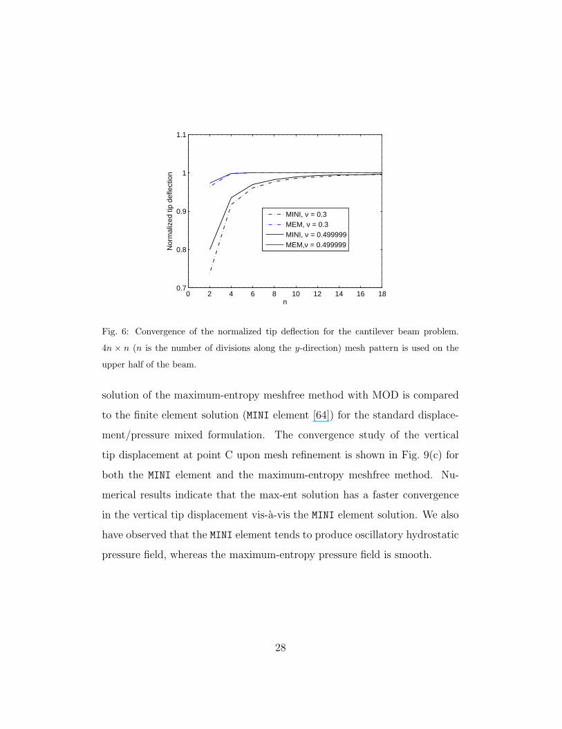
Fig. 6: Convergence of the normalized tip deflection for the cantilever beam problem.

4n × n (n is the number of divisions along the y-direction) mesh pattern is used on the

upper half of the beam.

solution of the maximum-entropy meshfree method with MOD is compared

to the finite element solution (MINI element [64]) for the standard displace-

ment/pressure mixed formulation. The convergence study of the vertical

tip displacement at point C upon mesh refinement is shown in Fig. 9(c) for

both the MINI element and the maximum-entropy meshfree method. Nu-

merical results indicate that the max-ent solution has a faster convergence

in the vertical tip displacement vis-a-vis the MINI element solution. We also

have observed that the MINI element tends to produce oscillatory hydrostatic

pressure field, whereas the maximum-entropy pressure field is smooth.

28

2 4 6 8 10 12 14 16 1810

−6

10−5

10−4

10−3

10−2

10−1

100

n

Ene

rgy

norm

of t

he e

rror

MEM, ν=0.3, STD (3 ngp), Rate = 1.12

MEM, ν=0.3, STD (6 ngp), Rate = 1.21

MEM, ν=0.3, STD (12 ngp), Rate = 1.17

MEM, ν=0.3, MOD, Rate = 1.12

(a)

2 4 6 8 10 12 14 16 1810

−6

10−5

10−4

10−3

10−2

10−1

100

n

Ene

rgy

norm

of t

he e

rror

MEM, ν=0.499999, STD (3 ngp)

MEM, ν=0.499999, STD (6 ngp), Rate = 0.95

MEM, ν=0.499999, STD (12 ngp), Rate = 1.21

MEM, ν=0.499999, MOD, Rate = 1.38

(b)

Fig. 7: Rate of convergence in energy norm for the cantilever beam problem using standard

and modified Gauss integration techniques. (a) ν = 0.3; and (b) ν = 0.499999. 4n× n (n

is the number of divisions along the y-direction) mesh pattern is used on the upper half

of the beam.

2 4 6 8 10 12 14 16 1810

−6

10−5

10−4

10−3

10−2

10−1

100

n

Ene

rgy

norm

of t

he e

rror

MINI, ν = 0.3, Rate = 0.94MEM, ν = 0.3, Rate = 1.44MINI, ν = 0.499999, Rate = 0.95MEM, ν = 0.499999, Rate = 1.38

Fig. 8: Rate of convergence in energy norm for the cantilever beam problem. 4n× n (n is

the number of divisions along the y-direction) mesh pattern is used on the upper half of

the beam.

29

48

A

B

C

F1644

24

(a) (b)

0 8 16 24 32 40 480

1

2

3

4

5

6

7

8

9

10

Divisions per side

Ver

tical

tip

disp

lace

men

t

MINI, ν = 0.4999MEM, ν = 0.4999

(c)

Fig. 9: Cook’s membrane problem. (a) Model geometry and boundary conditions; (b)

Sample mesh; and (c) Vertical tip displacement.

30

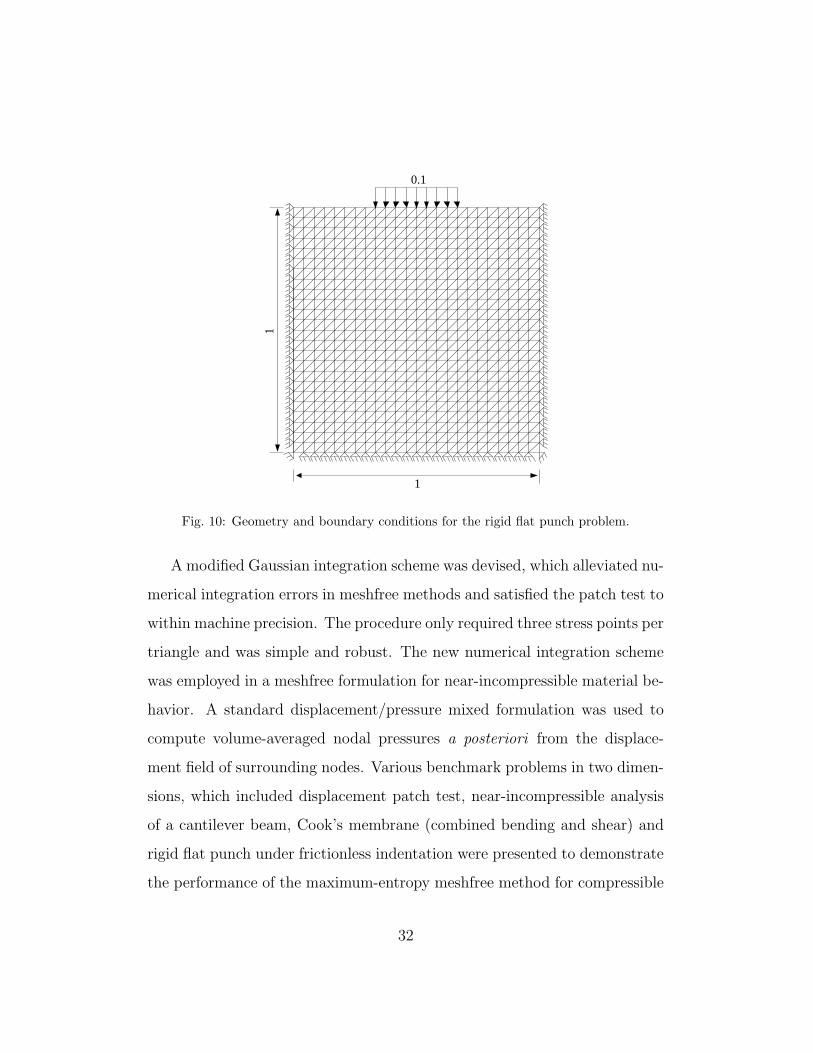
5.4. Rigid flat punch

As the last numerical example, we study the deformation of a square

block of dimensions 1 × 1 with unit thickness under plane strain state in

response to a frictionless indentation. A similar benchmark problem has

been considered in Refs. [65, 66, 67]. The bottom, left, and right edges

are fully clamped, which imposes a severe constraint on allowable deforma-

tion states when ν → 0.5. A downward displacement of 0.1 is applied over

the center portion of the top edge covering 1/3 of the edge’s length (see

Fig. 10). In the numerical computations the following parameters are spec-

ified: E = 107, ν = 0.499999. Maximum-entropy basis functions are used

with a support-width parameter γ = 1.5 for the quartic prior. In Figs. 11(a)

and 11(b), the numerical hydrostatic pressure field parameter is shown for

the maximum-entropy meshfree method within the standard displacement-

based formulation and for two different Gauss quadratures. As expected,

severe volumetric locking occurs. The corresponding maximum-entropy so-

lution for the volume-averaged nodal pressure formulation is presented in

Fig. 11(c), and we observe that the solution is free of volumetric locking and

spurious checkerboarding modes.

6. Concluding remarks

In this paper, a meshfree method for compressible and near-incompressible

elasticity based on maximum-entropy approximants was presented. The

adoption of maximum-entropy basis functions provides flexibility and eases

the implementation since it permits the direct imposition of essential bound-

ary conditions.

31

1

0.1

1

Fig. 10: Geometry and boundary conditions for the rigid flat punch problem.

A modified Gaussian integration scheme was devised, which alleviated nu-

merical integration errors in meshfree methods and satisfied the patch test to

within machine precision. The procedure only required three stress points per

triangle and was simple and robust. The new numerical integration scheme

was employed in a meshfree formulation for near-incompressible material be-

havior. A standard displacement/pressure mixed formulation was used to

compute volume-averaged nodal pressures a posteriori from the displace-

ment field of surrounding nodes. Various benchmark problems in two dimen-

sions, which included displacement patch test, near-incompressible analysis

of a cantilever beam, Cook’s membrane (combined bending and shear) and

rigid flat punch under frictionless indentation were presented to demonstrate

the performance of the maximum-entropy meshfree method for compressible

32

(a) (b)

(c)

Fig. 11: Rigid flat punch problem. (a), (b) MEM method with displacement-based lin-

ear elasticity and standard 3-point and 12-point Gauss quadrature, respectively; and (c)

MEM method with volume-averaged nodal pressure approach and modified integration

technique.

and near-incompressible elasticity. The numerical results revealed that the

maximum-entropy solution was devoid of volumetric locking and converged

optimally in the energy norm. The accurate numerical results in two di-

mensional linear elasticity point to the potential of the maximum-entropy

meshfree formulation in nonlinear and three-dimensional computations.

33

Appendix A

We prove that the modified Gauss quadrature scheme presented in Sec-

tion 4 exactly satisfies the patch test on a background mesh of three-node

triangles. To wit, it suffices to show that the nodal forces at all interior nodes

(whose basis function support vanish on the boundary) are identically equal

to zero for a uniform stress field σ = σc, i.e.,

fa =∑

e

∫

Ωe

BTaσ

c dΩ = 0 (A.1)

is to be established, where the assembly is over all elements e that have a

non-zero intersection with the support of φa.

Proof. From Eqs. (24) and (25), we can write the matrix Ba as

Ba(x) = Ba(x)− Ba +¯Ba = Ba(x)−

n∑

p=1

Ba(xp)wp +¯Ba,

and hence fa can be expressed as

fa =∑

e

∫

Ωe

[

BTa (x)−

n∑

p=1

BTa (xp)wp +

¯BTa

]

σc dΩ.

On performing numerical integration using n-point Gauss quadrature within

the element, we obtain

fa =∑

e

n∑

q=1

[

BTa (xq)−

n∑

p=1

BTa (xp)wp +

¯BTa

]

Aewqσc,

which simplifies to

fa =∑

e

n∑

q=1

¯BTaA

ewqσc,

34

since the first two terms cancel because∑n

q=1wq = 1 (Gauss weights sum to

unity). Recalling the expression for ¯Ba from Eq. (25), we have

fa =∑

e

n∑

q=1

3∑

L=1

m∑

r=1

¯NTa (ξr)|J(ξr)|wr

wqσc.

Now, closer inspection of the above equation and the expression for ¯Na given

in Eq. (24d) reveals that contribution along an interior edge L will arise

from two adjacent triangles with common edge L. However, since the normal

vector on the edge will assume equal magnitude but opposite signs for the

two cases, the two contributions cancel each other. Proceeding likewise, the

net contribution to fa from all interior edges vanishes, and hence Eq. (A.1)

is satisfied. 2

Acknowledgement

The authors (A. Ortiz and N. Sukumar) gratefully acknowledge the re-

search support of the National Science Foundation through contract grants

CMMI-0626481 and CMMI-0826513 to the University of California at Davis.

The work of M. A. Puso was performed under the auspices of the U.S.

Department of Energy by Lawrence Livermore National Laboratory under

Contract DE-AC52-07NA27344.

References

[1] T. J. R. Hughes, The Finite Element Method: Linear Static and Dy-

namic Finite Element Analysis, Dover Publications, Inc, Mineola, NY,

2000.

35

[2] T. J. R. Hughes, Generalization of selective integration procedures to

anisotropic and non-linear media, International Journal for Numerical

Methods in Engineering 15 (9) (1980) 1413–1418.

[3] D. S. Malkus, T. J. R. Hughes, Mixed finite element methods – reduced

and selective integration techniques: a unification of concepts, Computer

Methods in Applied Mechanics and Engineering 15 (1) (1978) 63–81.

[4] J. C. Simo, S. Rifai, A class of mixed assumed strain methods and

the method of incompatible modes, International Journal for Numerical

Methods in Engineering 29 (8) (1990) 1595–1638.

[5] B. Nayroles, G. Touzot, P. Villon, Generalizing the finite element

method: Diffuse approximation and diffuse elements, Computational

Mechanics 10 (1992) 307–318.

[6] T. Belytschko, Y. Y. Lu, L. Gu, Element-free Galerkin methods, Inter-

national Journal for Numerical Methods in Engineering 37 (2) (1994)

229–256.

[7] W. K. Liu, S. Jun, Y. F. Zhang, Reproducing kernel particle methods,

International Journal for Numerical Methods in Engineering 20 (8–9)

(1995) 1081–1106.

[8] T. J. Liszka, C. A. Duarte, W. W. Tworzydlo, hp-meshless cloud

method, Computer Methods in Applied Mechanics and Engineering

139 (1–4) (1996) 263–288.

[9] S. N. Atluri, T. Zhu, A new meshless local Petrov-Galerkin (MLPG)

36

approach in computational mechanics, Computational Mechanics 22 (2)

(1998) 117–127.

[10] N. Sukumar, B. Moran, T. Belytschko, The natural element method in

solid mechanics, International Journal for Numerical Methods in Engi-

neering 43 (5) (1998) 839–887.

[11] N. Sukumar, B. Moran, A. Y. Semenov, V. V. Belikov, Natural neigh-

bour Galerkin methods, International Journal for Numerical Methods

in Engineering 50 (1) (2001) 1–27.

[12] S. De, K. J. Bathe, The method of finite spheres, Computational Me-

chanics 25 (4) (2000) 329–345.

[13] M. Arroyo, M. Ortiz, Local maximum-entropy approximation schemes:

a seamless bridge between finite elements and meshfree methods, Inter-

national Journal for Numerical Methods in Engineering 65 (13) (2006)

2167–2202.

[14] A. Huerta, S. Fernandez-Mendez, Locking in the incompressible limit for

the element-free Galerkin method, International Journal for Numerical

Methods in Engineering 51 (11) (2001) 1361–1383.

[15] J. Dolbow, T. Belytschko, Volumetric locking in the element free

Galerkin method, International Journal for Numerical Methods in En-

gineering 46 (6) (1999) 925–942.

[16] D. Gonzalez, E. Cueto, M. Doblare, Volumetric locking in natural neigh-

bour Galerkin methods, International Journal for Numerical Methods in

Engineering 61 (4) (2004) 611–632.

37

[17] Y. Vidal, P. Villon, A. Huerta, Locking in the incompressible limit:

pseudo-divergence-free element free Galerkin, Communications in Nu-

merical Methods in Engineering 19 (9) (2003) 725–735.

[18] D. P. Recio, R. M. N. Jorge, L. M. S. Dinis, Locking and hourglass

phenomena in an element-free Galerkin context: the B-bar method with

stabilization and an enhanced strain method, International Journal for

Numerical Methods in Engineering 68 (13) (2006) 1329–1357.

[19] S. Beissel, T. Belytschko, Nodal integration of the element-free Galerkin

method, Computer Methods in Applied Mechanics and Engineering

139 (1) (1996) 49–74.

[20] J. S. Chen, C. T. Wu, S. Yoon, Y. You, A stabilized conforming nodal

integration for Galerkin mesh-free methods, International Journal for

Numerical Methods in Engineering 50 (2) (2001) 435–466.

[21] J. S. Chen, W. Hu, M. Puso, Orbital HP-clouds for solving Schrodinger

equation in quantum mechanics, Computer Methods in Applied Me-

chanics and Engineering 196 (37–40) (2007) 3693–3705.

[22] M. A. Puso, J. S. Chen, E. Zywicz, W. Elmer, Meshfree and finite

element nodal integration methods, International Journal for Numerical

Methods in Engineering 74 (3) (2008) 416–446.

[23] L. Kucherov, E. B. Tadmor, R. E. Miller, Umbrella spherical integration:

a stable meshless method for non-linear solids, International Journal for

Numerical Methods in Engineering 69 (13) (2007) 2807–2847.

38

[24] T. Belytschko, Y. Guo, W. K. Liu, S. P. Xiao, A unified stability anal-

ysis of meshless particle methods, International Journal for Numerical

Methods in Engineering 48 (9) (2000) 1359–1400.

[25] T. Belytschko, S. Xiao, Stability analysis of particle methods with

corrected derivatives, Computers and Mathematics with Applications

43 (3–5) (2002) 329–350.

[26] T. P. Fries, T. Belytschko, Convergence and stabilization of stress-point

integration in mesh-free and particle methods, International Journal for

Numerical Methods in Engineering 74 (7) (2008) 1067–1087.

[27] J. Dolbow, T. Belytschko, Numerical integration of Galerkin weak form

in meshfree methods, Computational Mechanics 23 (3) (1999) 219–230.

[28] M. Griebel, M. A. Schweitzer, A particle-partition of unity method. Part

II: Efficient cover construction and reliable integration, SIAM Journal

on Scientific Computing 23 (5) (2002) 1655–1682.

[29] T. Gerstner, M. Griebel, Numerical integration using sparse grids, Nu-

merical Algorithms 18 (3–4) (1998) 209–232.

[30] C. Riker, S. M. Holzer, The mixed-cell-complex partition-of-unity

method, Computer Methods in Applied Mechanics and Engineering

198 (13–14) (2009) 1235–1248.

[31] S. N. Atluri, H. G. Kim, J. Y. Cho, A critical assessment of the truly

meshless Local Petrov-Galerkin (MLPG), and Local Boundary Integral

Equation (LBIE) methods, Computational Mechanics 24 (5) (1999) 348–

372.

39

[32] S. De, K. J. Bathe, The method of finite spheres with improved numeri-

cal integration, Computers and Structures 79 (22–25) (2001) 2183–2196.

[33] M. Duflot, H. Nguyen-Dang, A truly meshless Galerkin method based

on a moving least squares quadrature, Communications in Numerical

Methods in Engineering 18 (6) (2002) 441–449.

[34] W. Zou, J. X. Zhou, Z. Q. Zhang, Q. Li, A truly meshless method based

on partition of unity quadrature for shape optimization of continua,

Computational Mechanics 39 (4) (2007) 357–365.

[35] Q.-H. Zeng, D.-T. Lu, Galerkin meshless methods based on partition

of unity quadrature, Applied Mathematics and Mechanics 26 (7) (2005)

893–899.

[36] A. Carpinteri, G. Ferro, G. Ventura, The partition of unity quadrature

in meshless methods, International Journal for Numerical Methods in

Engineering 54 (7) (2002) 987–1006.

[37] G. R. Balachandran, A. Rajagopal, S. M. Sivakumar, Mesh free Galerkin

method based on natural neighbors and conformal mapping, Computa-

tional Mechanics 42 (6) (2008) 885–905.

[38] G. R. Liu, Z. H. Tu, An adaptive procedure based on background cells

for meshless methods, Computer Methods in Applied Mechanics and

Engineering 191 (1) (2002) 1923–1943.

[39] I. Babuska, U. Banerjee, J. E. Osborn, Q. L. Li, Quadrature for meshless

methods, International Journal for Numerical Methods in Engineering

76 (9) (2008) 1434–1470.

40

[40] P. Schembri, D. L. Crane, J. N. Reddy, A three-dimensional compu-

tational procedure for reproducing meshless methods and the finite el-

ement method, International Journal for Numerical Methods in Engi-

neering 61 (6) (2004) 896–927.

[41] J. Bonet, A. J. Burton, A simple average nodal pressure tetrahedral ele-

ment for incompressible and nearly incompressible dynamic explicit ap-

plications, Communications in Numerical Methods in Engineering 14 (5)

(1998) 437–449.

[42] C. R. Dohrmann, M. W. Heinstein, J. Jung, S. W. Key, W. R.

Witkowski, Node-based uniform strain elements for three-node trian-

gular and four-node tetrahedral meshes, International Journal for Nu-

merical Methods in Engineering 47 (9) (2000) 1549–1568.

[43] R. L. Taylor, A mixed-enhanced formulation for tetrahedral finite el-

ements, International Journal for Numerical Methods in Engineering

47 (1–3) (2000) 205–227.

[44] J. Bonet, M. Marriot, O. Hassan, An averaged nodal deformation gra-

dient linear tetrahedral element for large strain explicit dynamic appli-

cations, Communications in Numerical Methods in Engineering 17 (8)

(2001) 551–561.

[45] F. M. Andrade Pires, E. A. de Souza Neto, J. L. de la Cuesta Padilla,

An assessment of the average nodal volume formulation for the analysis

of nearly incompressible solids under finite strains, Communications in

Numerical Methods in Engineering 20 (7) (2004) 569–583.

41

[46] M. A. Puso, J. Solberg, A stabilized nodally integrated tetrahedral, In-

ternational Journal for Numerical Methods in Engineering 67 (6) (2006)

841–867.

[47] G. Irving, C. Schroeder, R. Fedkiw, Volume conserving finite element

simulations of deformable models, ACM Transactions on Graphics 26 (3)

(2007) 13.1–13.6.

[48] P. Krysl, B. Zhu, Locking-free continuum displacement finite elements

with nodal integration, International Journal for Numerical Methods in

Engineering 76 (7) (2008) 1020–1043.

[49] J. C. Simo, T. J. R. Hughes, On the variational foundations of assumed

strain methods, Journal of Applied Mechanics 53 (1) (1986) 51–54.

[50] N. Sukumar, R. W. Wright, Overview and construction of meshfree ba-

sis functions: from moving least squares to entropy approximants, In-

ternational Journal for Numerical Methods in Engineering 70 (2) (2007)

181–205.

[51] C. E. Shannon, A mathematical theory of communication, The Bell

Systems Technical Journal 27 (1948) 379–423.

[52] E. T. Jaynes, Information theory and statistical mechanics, Physical

Review 106 (4) (1957) 620–630.

[53] N. Sukumar, Construction of polygonal interpolants: a maximum en-

tropy approach, International Journal for Numerical Methods in Engi-

neering 61 (12) (2004) 2159–2181.

42

[54] J. E. Shore, R. W. Johnson, Axiomatic derivation of the principle of

maximum entropy and the principle of minimum cross-entropy, IEEE

Transactions on Information Theory 26 (1) (1980) 26–36.

[55] S. Li, W. K. Liu, Meshfree and particle methods and their applications,

Applied Mechanics Reviews 55 (1) (2002) 1–34.

[56] T. P. Fries, H. G. Matthies, Classification and overview of meshfree

methods, Tech. Rep. Informatikbericht-Nr. 2003-03, Institute of Sci-

entific Computing, Technical University Braunschweig, Braunschweig,

Germany (2004).

[57] S. Fernandez-Mendez, A. Huerta, Imposing essential boundary condi-

tions in mesh-free methods, Computer Methods in Applied Mechanics

and Engineering 193 (12–14) (2004) 1257–1275.

[58] L. L. Yaw, N. Sukumar, S. K. Kunnath, Meshfree co-rotational formula-

tion for two-dimensional continua, International Journal for Numerical

Methods in Engineering 79 (8) (2009) 979–1003.

[59] C. J. Cyron, M. Arroyo, M. Ortiz, Smooth, second order, non-

negative meshfree approximants selected by maximum entropy, Inter-

national Journal for Numerical Methods in Engineering (2009) DOI:

10.1002/nme.2597.

[60] K. B. Nakshatrala, A. Masud, K. D. Hjelmstad, On finite element for-

mulations for nearly incompressible linear elasticity, Computational Me-

chanics 41 (4) (2008) 547–561.

43

[61] J. Yvonnet, P. Villon, F. Chinesta, Natural element approximations

involving bubbles for treating mechanical models in incompressible me-

dia, International Journal for Numerical Methods in Engineering 66 (7)

(2006) 1125–1152.

[62] N. Sukumar, E. A. Malsch, Recent advances in the construction of polyg-

onal finite element interpolants, Archives of Computational Methods in

Engineering 13 (1) (2006) 129–163.

[63] S. P. Timoshenko, J. N. Goodier, Theory of Elasticity, 3rd Edition,

McGraw-Hill, NY, 1970.

[64] D. N. Arnold, F. Brezzi, M. Fortin, A stable finite element for the Stokes

equations, Calcolo 21 (4) (1984) 337–344.

[65] E. A. de Souza Neto, F. M. Andrade Pires, D. R. J. Owen, F-bar-based

linear triangles and tetrahedra for finite strain analysis of nearly incom-

pressible solids. Part I: formulation and benchmarking, International

Journal for Numerical Methods in Engineering 62 (3) (2005) 353–383.

[66] P. Hauret, E. Kuhl, M. Ortiz, Diamond elements: a finite

element/discrete-mechanics approximation scheme with guaranteed op-

timal convergence in incompressible elasticity, International Journal for

Numerical Methods in Engineering 72 (3) (2007) 253–294.

[67] N. Kikuchi, Remarks on 4CST-elements for incompressible materials,

Computer Methods in Applied Mechanics and Engineering 37 (1) (1983)

109–123.

44