INTERNATIONAL JOURNAL FOR NUMERICAL METHODS IN FLUIDS

Int. J. Numer. Meth. Fluids 30: 1009–1026 (1999)

SIMULATION IN PRIMITIVE VARIABLES OFINCOMPRESSIBLE FLOW WITH PRESSURE NEUMANN

CONDITION

JULIO R. CLAEYSSENa,*, RODRIGO B. PLATTEa,1 AND ELBA BRAVOb,2

a Uni6ersidade Federal do Rio Grande do Sul, Instituto de Matematica-PROMEC-CESUP, PO Box 10673,90.001-000 Porto Alegre, RS, Brazil

b Uni6ersidade Regional Integrada-URI, Departamento de Engenharia e Ciencias da Computacao,98.400-000 Frederico Westphalen, RS, Brazil

SUMMARY

A velocity–pressure algorithm, in primitive variables and finite differences, is developed for incompress-ible viscous flow with a Neumann pressure boundary condition. The pressure field is initialized byleast-squares and updated from the Poisson equation in a direct weighted manner. Simulations with thecavity problem were made for several Reynolds numbers. The expected displacement of the central vortexwas obtained, as well as the development of secondary and tertiary eddies. Copyright © 1999 John Wiley& Sons, Ltd.

KEY WORDS: incompressible flow; primitive variables; velocity–pressure algorithm

1. INTRODUCTION

A velocity–pressure algorithm for incompressible viscous flow is developed in primitivevariables by using finite differences, a Neumann boundary condition for the pressure andwithout any iteration method for updating the pressure.

The incorporation of the Neumann condition for incompressible flow has been discussed indetail in a remarkable work by Gresho and Sani [1]. From a mathematical point of view, thesystem of equations governing an incompressible flow is singular with respect to the pressure.There is no evolutive equation for the pressure. In practice, the system is usually considered asthe momentum equation subject to a solenoidal restriction for the velocity field. The initial andboundary conditions are being prescribed only for the velocity field.

The discretization by difference methods of the Navier–Stokes equations on a staggered grid[23], when formulated in matrix terms, allows the identification of a singular evolutive matrixsystem. When the Poisson equation for the pressure is derived and its integration performed,it can be observed that a clear influence of the Neumann condition arises. From this, anon-singular system for determining the pressure values at the interior points can be extracted.The initialization process of the pressure, by a least-squares procedure, somehow incorporates

* Correspondence to: Universidade Federal do Rio Grande do Sul, Instituto de Matematica-PROMEC-CESUP, POBox 10673, 90.001-000 Porto Alegre, RS, Brazil. E-mail: julio@mat.ufrgs.br1 E-mail: rbplatte@mat.ufrgs.br2 E-mail: eoba@inf.uri.br

CCC 0271–2091/99/161009–19$17.50Copyright © 1999 John Wiley & Sons, Ltd.

Recei6ed 10 December 1997Re6ised 14 August 1998

J.R. CLAEYSSEN ET AL.1010

an optimal pressure as a starting point, instead of employing an arbitrary constant as it usuallydoes with iterative methods. The values of the velocity and pressure at interior points can bewell-determined by the forward Euler method for the velocity and by solving a non-singularPoisson equation without iteration. The latter means that the values of the pressure andvelocity are incorporated as soon as they are computed.

The formulation of the present algorithm follows the unified operator approach introducedby Casulli [2,20], which allows the consideration of, with minor modifications, the upwind andsemi-Lagrangean methods.

This velocity–pressure algorithm with central differences has been tested with the cavityflow problem for a wide range of Reynolds numbers. The displacement of the central vortexto the geometrical center of the cavity was obtained when increasing the Reynolds number, asearlier established by Burgggraf [3], Ghia et al. [4] and Schreiber and Keller [5] among others;also the development of secondary and tertiary vortices.

2. THE CONTINUUM EQUATIONS FOR INCOMPRESSIBLE FLOW

In this section a brief account of the prescription of the Neumann condition is given, asperformed by Gresho and Sani [1]. The Navier–Stokes equations for the velocity u(x, t) andpressure p(x, t) with initial and boundary conditions for the velocity, constitute the system

(u(t

+u ·9u+9p=n92u, t\0, (1)

9 ·u=0, (2)

u(x, 0)=u0(x), x in V( =V�G, (3)

u=w(x, t) in G=(V. (4)

Here V denotes a limited two-dimensional region, with G as its boundary, and

9 ·u0=0 in V (5)

is an initial solenoidal velocity field. From the above system, the initial normal velocity followsas

u0 ·n=w(x, 0)·n on G, (6)

and the global mass conservation as&G

u ·n dx=0. (7)

It is observed that no initial nor boundary conditions are prescribed for the pressure. Thus,p is determined up to an additive constant corresponding to the level of hydrostatic pressure.

The conditions of an initial velocity field solenoidal and normal velocity compatible with theabove boundary conditions are required for the problem to have a well-defined, unique andsolenoidal solution for all t]0 [6]. The initial tangential velocity field is not required to becompatible with the boundary conditions. If so, then the solution may be smoother [1].

By assuming adequate differentiability hypotheses, the Poisson equation can be derived bytaking the divergence of the momentum equation and using the vector identity

92u=9(9 ·u)−9×9×u. (8)

Copyright © 1999 John Wiley & Sons, Ltd. Int. J. Numer. Meth. Fluids 30: 1009–1026 (1999)

INCOMPRESSIBLE VISCOUS FLOW 1011

Therefore,

9 · (u ·9u)+92p=�

n92U−(U(t

�in V, (9)

where U=9 ·u.Since the prescribed conditions for u in G are valid everywhere in time, i.e.

9 ·u=0 in V( for t]0, (10)

they can be substituted into the equation for U and the Poisson equation for the pressure canbe obtained

92p= −9 · (u ·9u) in V for t]0. (11)

Consider the equivalent equation

92p=9 · (n92u−u ·9u). (12)

In order to complete the specification of the problem for the pressure, boundary conditionsshould be imposed for the pressure on G. Since the last two equations have been derived, theboundary conditions should be also derived. One obvious manner is to set the momentumequation as valid on the boundary. However, this is a vector equation and only one scalarboundary condition is required. Either the normal or the tangential projection of themomentum equation upon G can be chosen. The first option gives

n ·9p=(p(n

=n92un−�(un

(t+u ·9un

�in G for t]0. (13)

Thus, Equations (11), (12) and (13) constitute a Neumann problem for the pressure.On the other hand, the tangential component of the momentum equation upon G gives a

Dirichlet condition of type

t ·9p=(p(t

=n92ut−�(ut

(t+u ·9ut

�, (14)

where the value of p on G, i.e. Dirichlet data, is provided for by integration of (14) throught.

The determination of the solution of the Poisson equation (11) with Neumann boundaryconditions (13) requires holding the compatibility relationship&&

V92p dV=

&&V

−9 · (u ·9u) dV=7

Gpn dG, (15)

where pn=n ·9p and n is an exterior normal unit vector to G.

3. DISCRETIZATION OF THE NAVIER–STOKES EQUATIONS

For a non-dimensioned two-dimensional incompressible viscous flow, the primitive equationsare

(u(t

+u(u(x

+6(u(y

= −(p(x

+1

Re�(2u(x2+

(2u(y2

�, (16)

Copyright © 1999 John Wiley & Sons, Ltd. Int. J. Numer. Meth. Fluids 30: 1009–1026 (1999)

J.R. CLAEYSSEN ET AL.1012

(6

(t+u(6

(x+6(6

(y= −

(p(y

+1

Re�(26

(x2+(26

(y2

�, (17)

(u(x

+(6

(y=0, (18)

where u(x, y, t) and 6(x, y, t) denote the velocity components in the x- and y-directions,p(x, y, t) the pressure and Re]0 the Reynolds number respectively. This system can bewritten in the operator compact form

M(U(t

+NU= −PU+LU, (19)

where

U=ÃÆ

È

u6

pÃÇ

É, M=Ã

Æ

È

100

010

000ÃÇ

É,

N=ÃÃ

Ã

Ã

Ã

Æ

È

�u(

(x+6

(

(y�

0

0

0�u(

(x+6

(

(y�

0

0

0

0

ÃÃ

Ã

Ã

Ã

Ç

É

, P=ÃÃ

Ã

Ã

Ã

Æ

È

0

0

0

0

0

0

(

(x(

(y

0

ÃÃ

Ã

Ã

Ã

Ç

É

,

L=ÃÃ

Ã

Ã

Ã

Æ

È

1Re

� (2

(x2+(2

(y2

�0

(

(x

0

1Re

� (2

(x2+(2

(y2

�(

(y

0

0

0

ÃÃ

Ã

Ã

Ã

Ç

É

.

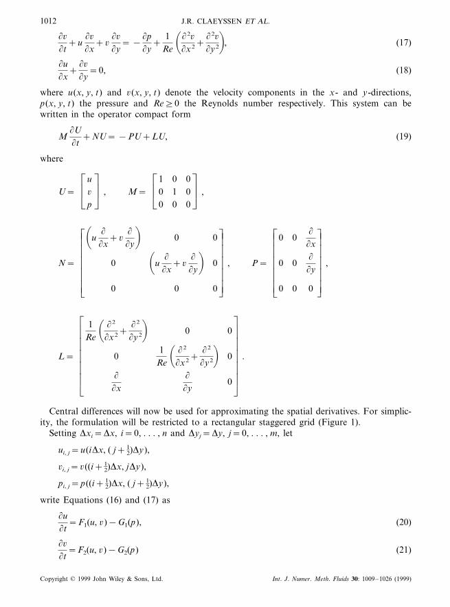
Central differences will now be used for approximating the spatial derivatives. For simplic-ity, the formulation will be restricted to a rectangular staggered grid (Figure 1).

Setting Dxi=Dx, i=0, . . . , n and Dyj=Dy, j=0, . . . , m, let

ui, j=u(iDx, ( j+12)Dy),

6i, j=6((i+12)Dx, jDy),

pi, j=p((i+12)Dx, ( j+1

2)Dy),

write Equations (16) and (17) as

(u(t

=F1(u, 6)−G1(p), (20)

(6

(t=F2(u, 6)−G2(p) (21)

Copyright © 1999 John Wiley & Sons, Ltd. Int. J. Numer. Meth. Fluids 30: 1009–1026 (1999)

INCOMPRESSIBLE VISCOUS FLOW 1013

respectively, then apply spatial central differences. It turns out that

F1(u, 6)= −ui, j

ui+1, j−ui−1, j

2Dx−6 �ui, j

ui, j+1−ui, j−1

2Dy

+1

Re�ui+1, j−2ui, j+ui−1, j

Dx2 +ui, j+1−2ui, j+ui, j−1

Dy2

�, (22)

F2(u, 6)= −u �6i, j

6i+1, j−6i−1, j

2Dx−6i, j

6i, j+1−6i, j−1

2Dy

+1

Re�6i+1, j−26i, j+6i−1, j

Dx2 +6i, j+1−26i, j+6i, j−1

Dy2

�. (23)

Similarly,

G1(p)=pi, j−pi−1, j

Dx, (24)

G2(p)=pi, j−pi, j−1

Dy. (25)

Here 6 �ui, jand u �6i, j

denote the average values

6 �ui, j=6i, j+1+6i, j+6i+1, j+1+6i+1, j−1

4(26)

and

u �6i, j=

ui, j+1+ui, j+ui+1, j+1+ui+1, j+1

4. (27)

3.1. Matrix formulation

The above spatial discretization procedure, together with the pressure Neumann condition,for the Navier–Stokes equations on a rectangular staggered grid amounts, in matrix terms, toreplace (19) by the spatial approximation [17]

Figure 1. Staggered grid.

Copyright © 1999 John Wiley & Sons, Ltd. Int. J. Numer. Meth. Fluids 30: 1009–1026 (1999)

J.R. CLAEYSSEN ET AL.1014

MdU

dt+N(U)U+NF(U, UF)UF= −PU−PF(U, UF)+LU+LFUF. (28)

Here U= [Ui,j ], where Ui,j includes the values ui+1/2,j, 6i,j+1/2, pi,j at a cell (i, j ). The vectorUF corresponds to the boundary values of u, 6 and p. The matrices M, N, L, P are thecorresponding spatial approximation of the continuous terms and NF, LF, PF are matrices thatcontain boundary values. The above systems are singular once M is a singular matrix [18].

If an upwind approximation is used for the velocity field and central differences are kept forthe pressure gradient, it will turn out that the matrix formulation reads [19],

MdU

dt+N(U, UF)U+NF(U, UF)UF= −PU−PF(U, UF)+LU+LFUF. (29)

From such equations, it is observed that although the N matrix is different for each method,there is a direct influence of boundary values on the non-linear convection matrix whendiscretized by the upwind method. This is not the case for central differences, and in numericalterms it means that boundary values do not interfere with the numerical convection at interiorpoints.

The above matrix formulation will be of a similar nature for non-rectangular domains.

3.2. Time discretization

The time discretization of the momentum equations, besides modifying the order ofapproximation, raises numerical stability problems. Although implicit methods have betterstability properties, they are expensive to implement. In this paper, the explicit Euler orAdams–Bashforth methods will be used.

The Adams–Bashforth method, applied to Equations (20) and (21), can be written as

uk+1=uk+Dt %np−1

l=0

al [F1(u, 6)−G1(p)], (30)

6k+1=6k+Dt %np−1

l=0

al [F2(u, 6)−G2(p)], (31)

where k= t/Dt represents the time steps and the coefficients np and a1 define a specific method:np=1, a0=1 (first-order forward Euler); np=2, a0=

32, a1= −1

2 (second-order Adams–Bash-forth); and np=3, a0=

2312, a1= −4

3, a2=512 (third-order Adams–Bashforth).

4. THE CORRECTED PRESSURE EQUATION

Gresho and Sani [1] derived an equation for pressure in such a way that for 9 ·u0=0, thesystem given by Equations (1) and (2) can be replaced by

(u(t

+u ·9u+9p=1

Re92u, (32)

92p=9 ·� 1

Re92u−u ·9u

�, (33)

where the boundary condition for p is given by

n ·9p=(p(n

=1

Re92un−

�(un

(t+u ·9un

�for t]0. (34)

Copyright © 1999 John Wiley & Sons, Ltd. Int. J. Numer. Meth. Fluids 30: 1009–1026 (1999)

INCOMPRESSIBLE VISCOUS FLOW 1015

The discretization of the pressure equation, being a derived one, requires special care inorder to control the accumulation of numerical errors that might invalidate the continuityequation. This means there is a need to introduce corrective terms into the pressure equation.

Consider the momentum equations discretized as

ui, jk+1=ui, j

k +Dt %np+1

l=0

al [F(ui, jk− l)−9pi, j

k− l], (35)

where np and a1 depend upon the employed Adams–Bashforth method, F(uk) being thediscretization operator of the convective and diffusive terms.

Applying the divergence operator to both sides of (35) results in

9 ·ui, jk+1=9 ·ui, j

k +Dt %np−1

l=0

al [9 ·F(ui, jk− l)−92pi, j

k− l]. (36)

The incompressibility condition at the (k+1)th time step, 9 ·uk+1=0, is then characterizedby

92pi, jk =9 ·F(ui, j

k− l)+9 ·ui, j

k+1

a0Dt+

1a0

%np−1

l=0

al [9 ·F(ui, jk− l)−92pi, j

k− l]. (37)

It is observed that, for the Euler method, the above correction coincides with the dilatationterm Dt=9 ·un/Dt [7–9].

Equation (37) can be written in the compact form

92pk=9 ·H(uk), (38)

where

H(uk)=F(uk)+uk

a0Dt+

1a0

%np−1

l=0

al [F(uk− l)−9pk− l]. (39)

Now, the Laplacian of the pressure is discretized with second-order central differences on astaggered grid

92pi, j:pi−1, j+pi, j−1−4pi, j+pi+1, j+pi, j+1

h2 , (40)

where h=Dx=Dy. Thus, Equation (38) becomes

pi−1, j+pi, j−1−4pi, j+pi+1, j+pi, j+1=h(H1i+1, j−H1i, j

+H2i, j−H2i, j

), (41)

where H1i,jand H2i,j

are the x and y components of H(u) respectively, applied at the points(iDx, ( j+1

2)Dy) for the first component and ((i+12)Dx, jDy) for the second one.

For good convergence of the discretized Poisson equation with a Neumann condition, thecompatibility relationship (15) must hold exactly on the discretized domain, i.e. [10,16]

%i, j�V

92pi, j= %i, j�G

(pi, j

(h. (42)

By adding (41) for all points of the square domain, you have

%n−1

i=1

%m−1

j=1

pi−1, j+pi, j−1−4pi, j+pi+1, j+pi, j+1

=h %n−1

i=1

%m−1

j=1

H1i+1, j−H1i, j

+H2i, j+1−H2i, j

, (43)

Copyright © 1999 John Wiley & Sons, Ltd. Int. J. Numer. Meth. Fluids 30: 1009–1026 (1999)

J.R. CLAEYSSEN ET AL.1016

and by making simplifications, you obtain

%m−1

j=1

(p0, j−p1, j−pn−1, j+pn, j)+ %n−1

i=1

(pi,0−pi,1−pi,m−1+pi,m)

=h %m−1

j=1

(H1n, j−H11, j

)+h %n−1

i=1

(H2i,m−H2i,1

). (44)

Then the discrete Neumann condition holds for

p0, j=p1, j−hH11, j, (45)

pn, j=pn−1, j+hH1n, j, (46)

pi,0=pi,1−hH2i,1, (47)

pi,m=pi,m−1+hH2i,m. (48)

It should be observed that these boundary conditions are discretizations of (34).

5. THE VELOCITY–PRESSURE ALGORITHM

An algorithm for integrating the Navier–Stokes equations is now presented. First, the pressureis initialized by solving a singular system that arises from the discretization of the pressureequation with the Neumann conditions. Second, the momentum equations are solved for thevelocity field at each time step. Third, the pressure is updated by solving a Poisson equation,giving a special treatment for the interior points that correspond to interior cells and to theadjacent cells in such a way that the compatibility condition is verified. This updating containscorrective terms for the direct calculation of the pressure at interior points of interior cells.This is done by incorporating the already known pressure values at neighboring points.

5.1. Pressure initialization

To initialize the pressure, Equation (38) is considered with k=0

92p0=9 ·H(u0). (49)

Here we use np=1 and a0=1, as 9 ·u0=0, H(u0)=F(u0). No corrective term appears on theinitialization, and the discretize boundary conditions are (45)–(48).

Equation (49), discretized as in (41) associated to the boundary conditions, when written inmatrix terms is

Ap0=b, (50)

where A is the singular matrix

A=ÃÃ

Ã

Ã

Ã

Æ

È

S1

II

S2

II

S2

· · ·

I· · ·I

· · ·S2

II

S1

ÃÃ

Ã

Ã

Ã

Ç

É(m×n)× (m×n)

,

Copyright © 1999 John Wiley & Sons, Ltd. Int. J. Numer. Meth. Fluids 30: 1009–1026 (1999)

INCOMPRESSIBLE VISCOUS FLOW 1017

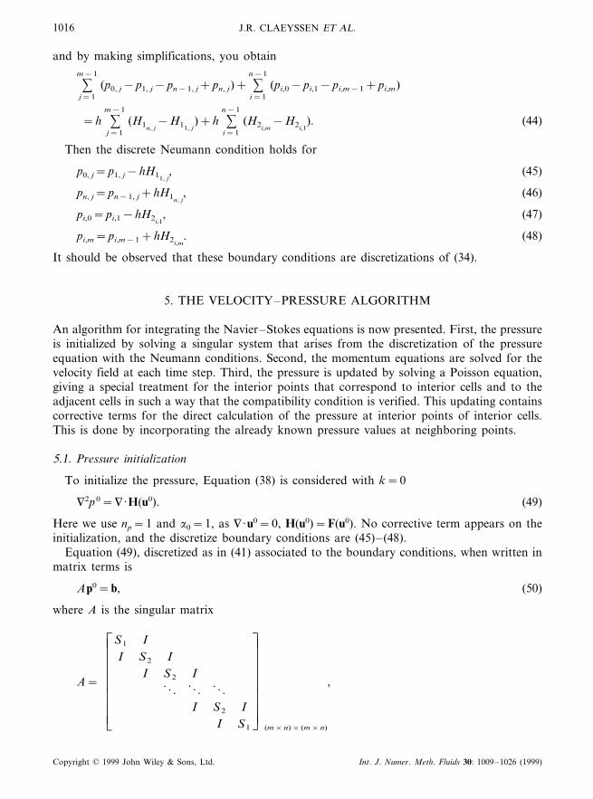
Figure 2. Pressure molecule.

with

S1=ÃÃ

Ã

Æ

È

−21

1−3· · ·

1· · ·1

· · ·−31

1−2

ÃÃ

Ã

Ç

Én×n

, S2=ÃÃ

Ã

Æ

È

−31

1−4· · ·

1· · ·1

· · ·−41

1−3

ÃÃ

Ã

Ç

Én×n

and I is the identity matrix of order n.At time k=0, the vector p0 contains the values of the pressure at interior points, i.e.

p0= [p1,10 p2,1

0 · · ·pn,10 p1,2

0 · · ·p2,20 · · ·pn,2

0 · · ·p1,m0 p2,m

0 · · ·pn,m0 ]T.

The vector b contains all values ni,j0 , 6 i,j

0 from the right-hand-side of (45)–(48), which aregiven initial values, and this has the particular form

b= [0· · ·0 bmn−n+1 0· · ·0 bmn ]m×nT ,

where

bmn−n+1=2n

hand bmn= −

2n

h.

Hence, b is a non-zero vector.The above singular system can be solved by several methods: least-squares, iterative or LU

[25,22,21].

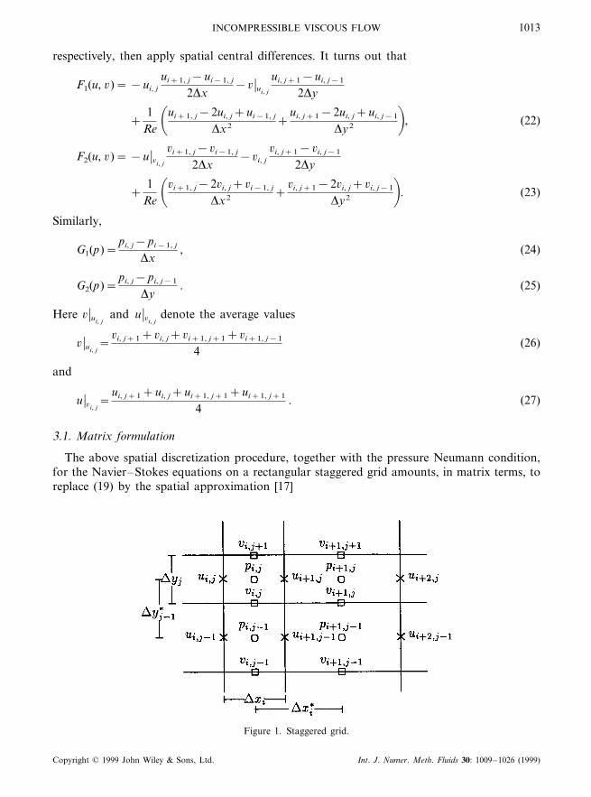
5.2. The one-step pressure updating

Once the pressure is initialized, the interior pressure values pi,j at time t+Dt are computedwith the following one-step and explicit scheme (Figure 2):

pi, jk+1=

14

[pi−1, jk+1 +pi, j−1

k+1 +pi+1, jk +pi, j+1

k ]−h2

49 ·H(ui, j

k+1), (51)

which incorporates by simple averaging, old and new values for the pressure.This updating of the pressure field can written in matrix terms as

Bpk+1+Cpk= −Q(uk+1), (52)

where

Copyright © 1999 John Wiley & Sons, Ltd. Int. J. Numer. Meth. Fluids 30: 1009–1026 (1999)

J.R. CLAEYSSEN ET AL.1018

B=ÃÃ

Ã

Æ

È

B1

I B1

I B1

· · ·· · ·I B1

ÃÃ

Ã

Ç

É

and C=ÃÃ

Ã

Æ

È

C1 IC1 I

C1· · ·· · · I

C1

ÃÃ

Ã

Ç

É

,

with

B1=ÃÃ

Ã

Æ

È

−41 −4

1 −4· · ·

· · ·1 −4

ÃÃ

Ã

Ç

É

and C1=ÃÃ

Ã

Æ

È

0 10 1

0 · · ·· · · 1

0

ÃÃ

Ã

Ç

É

,

where B and C are matrices of order ((m−2)× (n−2))× ((m−2)× (n−2)), B1 and C1 oforder (n−2)× (n−2) and I is the identity matrix of order (n−2).

The term Q(uk+1) contains the velocity and corrective terms of (51). The above matrixequation for updating the pressure must not be considered as being iterative. It is just acompact form of writing (51).

5.3. Velocity–pressure algorithm

The algorithm for solving an incompressible viscous flow with prescribed Neumann condi-tions for the pressure is given as follows:

1. Introduction of the initial velocity components at time t0=0, corresponding to level k=0,and the boundary conditions for the velocity field.

2. Initialization of the pressure by solving a singular linear system of the type

Ap0=b

through least-squares, iterative or LU decomposition.3. Computation of the velocity field ui,j

k+1 and 6 i,jk+1 by using (30) and (31) respectively.

4. Computation of the pressure p at time level k+1 through (51).5. Updating of the pressure and velocity field by setting pk+1 instead of pk and uk+1 instead

of uk.6. Perform steps (3)–(5) for k=1, 2, . . .7. End the calculations.

Remarks

1. This algorithm computes corrected pressure values at interior points without any iteration.2. The algorithm can handle non-rectangular geometries. The only modifications are related

to boundary rows and columns of matrices A, B and C, the non-linear term Q and theinitial vector b. In this work, for simplicity and numericals with a broad range of Re, thealgorithm was set up from a two-dimensional square cavity discussion. However, simula-tions were made for cavities with a non-rectangular bottom.

3. The above algorithm have been successfully employed with three-dimensional rotatingconvective flow and with the inclusion of viscoelastic terms. It is a matter of a forthcomingpaper.

Copyright © 1999 John Wiley & Sons, Ltd. Int. J. Numer. Meth. Fluids 30: 1009–1026 (1999)

INCOMPRESSIBLE VISCOUS FLOW 1019

5.4. Extension to three-dimensional domains

The case of a three-dimensional cubic cavity can be easily handled. For a velocity fieldu= (u, 6, w) on a staggered grid, consider

uix,iy,iz=u(ixDx, (iy+

12)Dy, (iz+

12)Dz),

6ix,iy,iz=6((ix+1

2)Dx, iyDy, (iz+12)Dz),

wix,iy,iz=w((ix+1

2)Dx(iy+12)Dy, izDz),

pix,iy,iz=p((ix+1

2)Dx, (iy+12)Dy, (iz+

12)Dz).

The discretized momentum equations read

uix,iy,izk+1 =uix,iy,iz

k +Dt %np−1

l=0

al [F(uix,iy,izk−1 )−9pix,iy,iz

k−1 ], (53)

where the operator F has a similar meaning to that in the two-dimensional case.The equation for the pressure. including correcting terms, becomes

92pix,iy,izk =9 ·F(uix,iy,iz

k )+9 ·uix,iy,iz

k

a0Dt+

1a0

%np−1

l=0

al [9 ·F(uix,iy,izk− l )−92pix,iy,iz

k− l ]. (54)

The discretization of the Laplacian operator on a cubic cavity by second-order centraldifferences and the fulfillment of the discrete compatibility relationship lead to the one-stepand explicit scheme

pix,iy,izk+1 =

16

[pix−1,iy,izk+1 +pix,iy−1,iz

k+1 +pix,iy,iz−1k+1 +pix+1,iy,iz

k +pix,iy+1,izk +pix,i,iz+1

k ]

−h2

69 ·H(uix,iy,iz

k ), (55)

where

H(uk)=F(uk)+uk

a0Dt+

1a0

%np−1

l=1

al [F(uk− l)−9pk−1]. (56)

Here h=Dx=Dy=Dz.

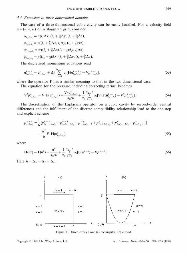
Figure 3. Driven cavity flow: (a) rectangular; (b) curved.

Copyright © 1999 John Wiley & Sons, Ltd. Int. J. Numer. Meth. Fluids 30: 1009–1026 (1999)

J.R. CLAEYSSEN ET AL.1020

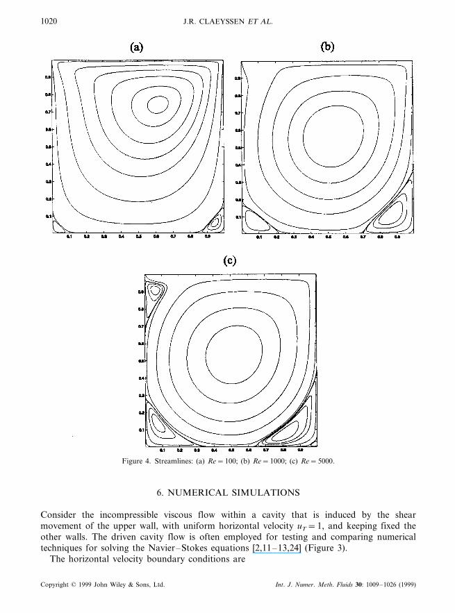
Figure 4. Streamlines: (a) Re=100; (b) Re=1000; (c) Re=5000.

6. NUMERICAL SIMULATIONS

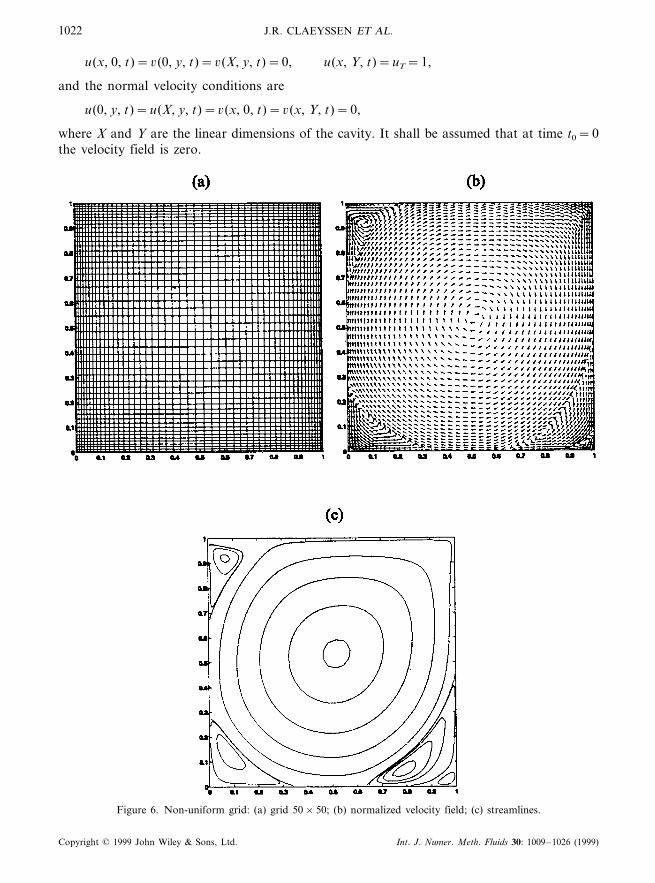
Consider the incompressible viscous flow within a cavity that is induced by the shearmovement of the upper wall, with uniform horizontal velocity uT=1, and keeping fixed theother walls. The driven cavity flow is often employed for testing and comparing numericaltechniques for solving the Navier–Stokes equations [2,11–13,24] (Figure 3).

The horizontal velocity boundary conditions are

Copyright © 1999 John Wiley & Sons, Ltd. Int. J. Numer. Meth. Fluids 30: 1009–1026 (1999)

INC

OM

PR

ESSIB

LE

VISC

OU

SF

LO

W1021

Copyright

©1999

JohnW

iley&

Sons,L

td.Int.

J.N

umer.

Meth.

Fluids

30:1009

–1026

(1999)

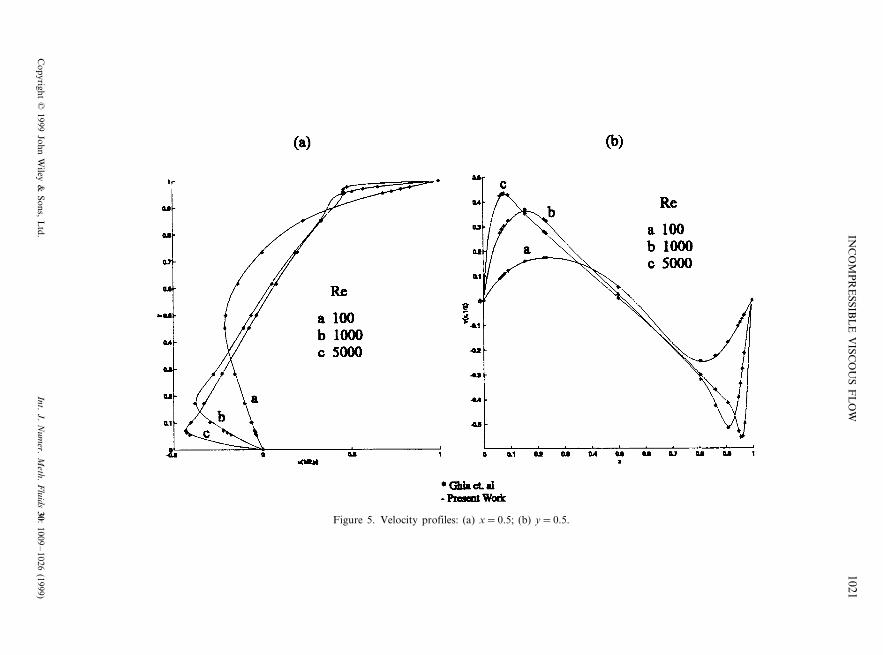
Figure 5. Velocity profiles: (a) x=0.5; (b) y=0.5.

J.R. CLAEYSSEN ET AL.1022

u(x, 0, t)=6(0, y, t)=6(X, y, t)=0, u(x, Y, t)=uT=1,

and the normal velocity conditions are

u(0, y, t)=u(X, y, t)=6(x, 0, t)=6(x, Y, t)=0,

where X and Y are the linear dimensions of the cavity. It shall be assumed that at time t0=0the velocity field is zero.

Figure 6. Non-uniform grid: (a) grid 50×50; (b) normalized velocity field; (c) streamlines.

Copyright © 1999 John Wiley & Sons, Ltd. Int. J. Numer. Meth. Fluids 30: 1009–1026 (1999)

INCOMPRESSIBLE VISCOUS FLOW 1023

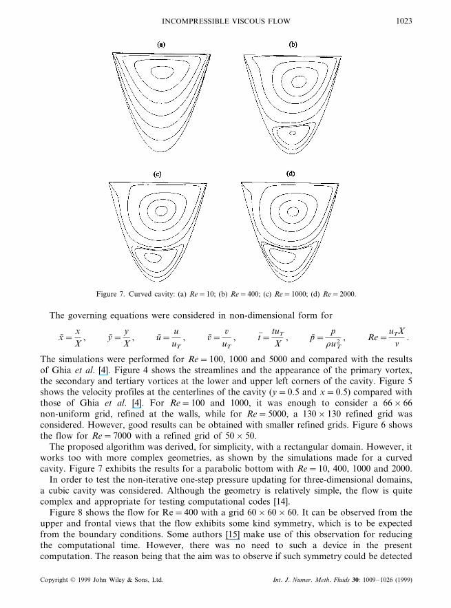
Figure 7. Curved cavity: (a) Re=10; (b) Re=400; (c) Re=1000; (d) Re=2000.

The governing equations were considered in non-dimensional form for

x=xX

, y=yX

, u=uuT

, 6=6

uT

, t( = tuT

X, p=

pruT

2 , Re=uTX

n.

The simulations were performed for Re=100, 1000 and 5000 and compared with the resultsof Ghia et al. [4]. Figure 4 shows the streamlines and the appearance of the primary vortex,the secondary and tertiary vortices at the lower and upper left corners of the cavity. Figure 5shows the velocity profiles at the centerlines of the cavity (y=0.5 and x=0.5) compared withthose of Ghia et al. [4]. For Re=100 and 1000, it was enough to consider a 66×66non-uniform grid, refined at the walls, while for Re=5000, a 130×130 refined grid wasconsidered. However, good results can be obtained with smaller refined grids. Figure 6 showsthe flow for Re=7000 with a refined grid of 50×50.

The proposed algorithm was derived, for simplicity, with a rectangular domain. However, itworks too with more complex geometries, as shown by the simulations made for a curvedcavity. Figure 7 exhibits the results for a parabolic bottom with Re=10, 400, 1000 and 2000.

In order to test the non-iterative one-step pressure updating for three-dimensional domains,a cubic cavity was considered. Although the geometry is relatively simple, the flow is quitecomplex and appropriate for testing computational codes [14].

Figure 8 shows the flow for Re=400 with a grid 60×60×60. It can be observed from theupper and frontal views that the flow exhibits some kind symmetry, which is to be expectedfrom the boundary conditions. Some authors [15] make use of this observation for reducingthe computational time. However, there was no need to such a device in the presentcomputation. The reason being that the aim was to observe if such symmetry could be detected

Copyright © 1999 John Wiley & Sons, Ltd. Int. J. Numer. Meth. Fluids 30: 1009–1026 (1999)

J.R. CLAEYSSEN ET AL.1024

with the proposed non-iterative pressure algorithm, which does not need to update the pressurein a symmetric way.

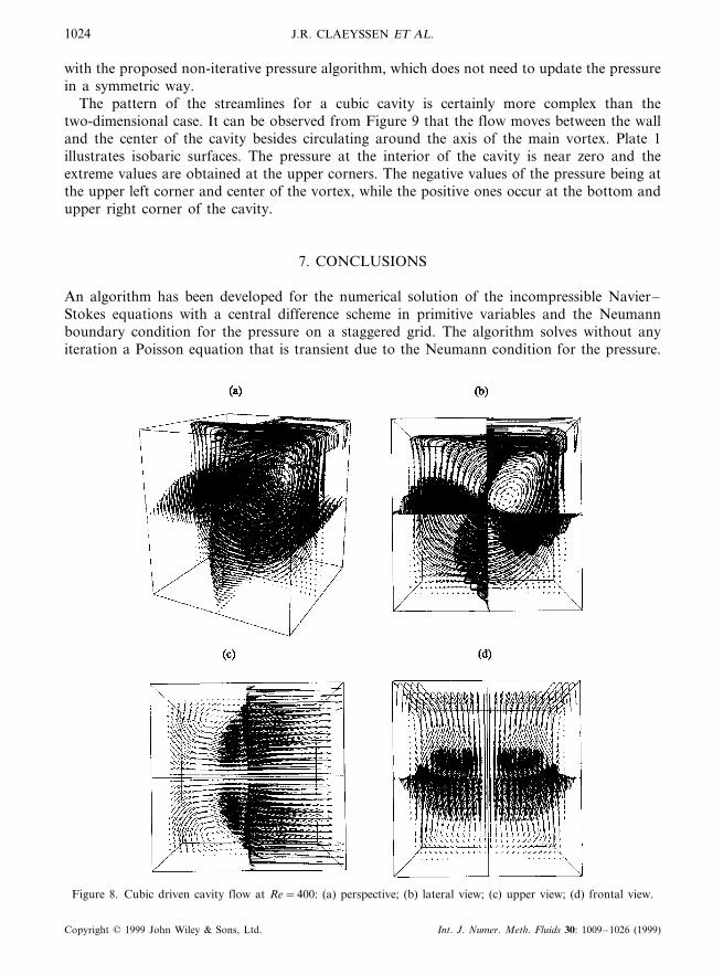
The pattern of the streamlines for a cubic cavity is certainly more complex than thetwo-dimensional case. It can be observed from Figure 9 that the flow moves between the walland the center of the cavity besides circulating around the axis of the main vortex. Plate 1illustrates isobaric surfaces. The pressure at the interior of the cavity is near zero and theextreme values are obtained at the upper corners. The negative values of the pressure being atthe upper left corner and center of the vortex, while the positive ones occur at the bottom andupper right corner of the cavity.

7. CONCLUSIONS

An algorithm has been developed for the numerical solution of the incompressible Navier–Stokes equations with a central difference scheme in primitive variables and the Neumannboundary condition for the pressure on a staggered grid. The algorithm solves without anyiteration a Poisson equation that is transient due to the Neumann condition for the pressure.

Figure 8. Cubic driven cavity flow at Re=400: (a) perspective; (b) lateral view; (c) upper view; (d) frontal view.

Copyright © 1999 John Wiley & Sons, Ltd. Int. J. Numer. Meth. Fluids 30: 1009–1026 (1999)

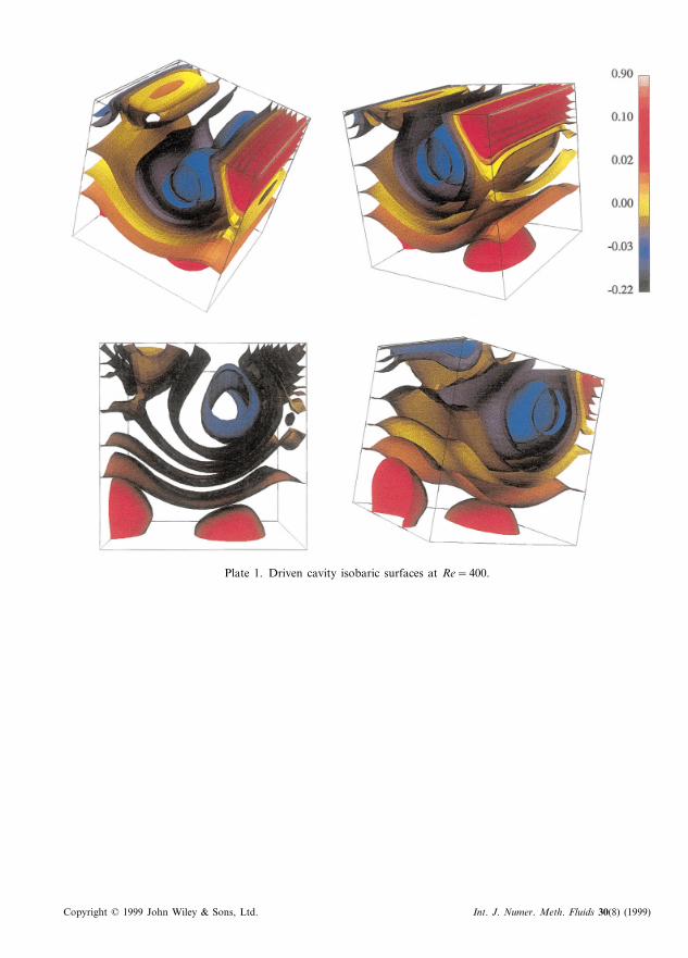
Plate 1. Driven cavity isobaric surfaces at Re=400.

Copyright © 1999 John Wiley & Sons, Ltd. Int. J. Numer. Meth. Fluids 30(8) (1999)

INCOMPRESSIBLE VISCOUS FLOW 1025

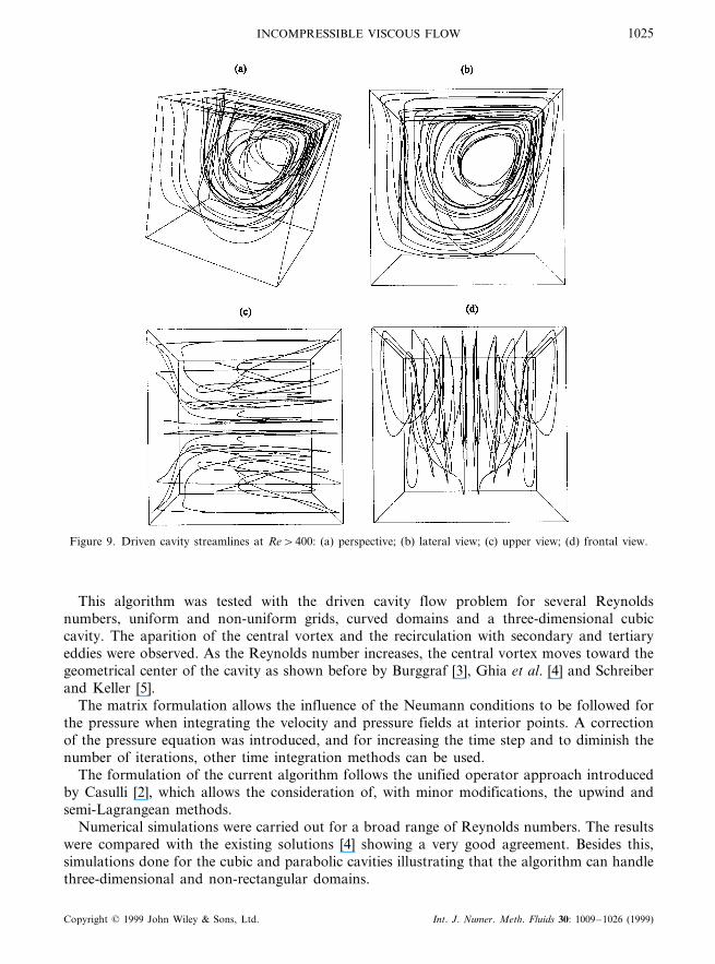
Figure 9. Driven cavity streamlines at Re\400: (a) perspective; (b) lateral view; (c) upper view; (d) frontal view.

This algorithm was tested with the driven cavity flow problem for several Reynoldsnumbers, uniform and non-uniform grids, curved domains and a three-dimensional cubiccavity. The aparition of the central vortex and the recirculation with secondary and tertiaryeddies were observed. As the Reynolds number increases, the central vortex moves toward thegeometrical center of the cavity as shown before by Burggraf [3], Ghia et al. [4] and Schreiberand Keller [5].

The matrix formulation allows the influence of the Neumann conditions to be followed forthe pressure when integrating the velocity and pressure fields at interior points. A correctionof the pressure equation was introduced, and for increasing the time step and to diminish thenumber of iterations, other time integration methods can be used.

The formulation of the current algorithm follows the unified operator approach introducedby Casulli [2], which allows the consideration of, with minor modifications, the upwind andsemi-Lagrangean methods.

Numerical simulations were carried out for a broad range of Reynolds numbers. The resultswere compared with the existing solutions [4] showing a very good agreement. Besides this,simulations done for the cubic and parabolic cavities illustrating that the algorithm can handlethree-dimensional and non-rectangular domains.

Copyright © 1999 John Wiley & Sons, Ltd. Int. J. Numer. Meth. Fluids 30: 1009–1026 (1999)

J.R. CLAEYSSEN ET AL.1026

REFERENCES

1. P.M. Gresho and R.L. Sani, ‘On pressure boundary conditions for the incompressible Navier–Stokes equations’,Int. J. Numer. Methods Fluids, 7, 1111–1145 (1987).

2. V. Casulli, ‘Eulerian–Lagrangian Methods for the Navier–Stokes equations at high Reynolds number’, Int. J.Numer. Methods Fluids, 8, 1349–1360 (1988).

3. O.R. Burggraf, ‘Analytical and numerical studies of the structure of steady separated flows’, J. Fluid Mech., 24,113–151 (1966).

4. U. Ghia, K.N. Ghia and C.T. Shin, ‘High-Re solutions for incompressible flow using the Navier–Stokes equationsand a multigrid method’, J. Comput. Phys., 48, 387–411 (1982).

5. R. Schreiber and H.B. Keller, ‘Driven cavity flows by efficient numerical techniques’, J. Comput. Phys., 49,310–333 (1983).

6. R. Temam, Na6ier–Stokes Equations, 3rd. edn., North-Holland, Amsterdam, 1985.7. W.F. Ames, Numerical Methods for Partial Differential Equations, 3rd edn., Academic Press, San Diego, 1992.8. J.H. Ferziger and M. Peric, Computational Methods for Fluid Dynamics, Springer, Berlin, 1996.9. P.J. Roache, Computational Fluid Dynamic, Hermosa, Albuquerque, NM, 1982.

10. S. Abdallah, ‘Numerical solutions for the pressure Poisson equation with Neumann boundary conditions using anon-staggered grid, I’, J. Comput. Phys., 70, 182–192 (1987).

11. A.T. Degani and G.C. Fox, ‘Parallel multigrid computation of the unsteady incompressible Navier–stokesequations’, J. Comput. Phys., 128, 223–236 (1996).

12. M.M. Gupta, ‘High accuracy solutions of incompressible Navier–Stokes equations’, J. Comput. Phys., 93,343–359 (1991).

13. S. Hou, Q. Zou, S. Chen, G. Doolen and A.C. Cogley, ‘Simulation of flow by the lattice Boltzmann method’, J.Comput. Phys., 118, 329–347 (1995).

14. W.T. Wang and T.H. Sheu, ‘An element-by-element BIGGSTAB iterative method for three-dimensional steadyNavier–Stokes equations’, J. Comput. Appl. Math., 79, 147–165 (1997).

15. X.H. Wu, J.Z. Wu and J.M. Wu, ‘Effective vorticity–velocity formulations for three-dimensional incompressibleviscous flows’, J. Comput. Phys., 122, 68–82 (1995).

16. B.J. Alfrink, ‘On the Neumann problem for the pressure in a Navier–Stokes model’, Proc. 2nd Int. Conf. onNumerical Methods in Laminar and Turbulent Flow, Venice, 1981, pp. 389–399.

17. E. Bravo and J.R. Claeyssen, ‘Simulacao central pare escoamento incompressıvel em variaveis primitivas econdicoes de Neumann para a pressao’, XIX Cong. Nacional de Matematica Aplicada e Computacional-CNMAC,Goiania, Brasil, 1996.

18. K.E. Brenam, S.L. Campbell, and L.R. Petzold, Numerical Solution of Initial Value Problems in Differential–Alge-braic Equations, Elsevier Science Publishing, New York, 1989.

19. A. Castro, and Bravo, ‘Upwind simulation of an incompressible flow with natural pressure boundary conditionon a staggered grid’, SIAM Annual Meeting, Kansas City, USA, 1996.

20. V. Casulli, ‘Eulerian–Lagrangian methods for hyperbolic and convection dominated parabolic problems’, in C.Taylor, D.R.J. Owen and E. Hinton (eds.), Computational Methods for Non-Linear Problems, Pineridge Press,Swansea, 1987, pp. 239–269.

21. J.R. Claeyssen and H.F. Campos Velho, ‘Initialization using non-modal matrix for a limited area model’, BoletimSBMAC, 4, 41–48 (1994).

22. B.N. Datta, Numerical Linear Algebra and Applications, Brooks/Cole Publishing Company, Monterey, CA, 1995.23. F.H. Harlow and J.E. Welsh, ‘Numerical calculation of time dependent viscous incompressible flow with free

surface’, Phys. Fluids, 8, 2182–2189 (1965).24. G. Mansell, J. Walter and E. Marschal, ‘Liquid–liquid driven cavity flow’, J. Comput. Phys., 110, 274–284 (1994).25. C.R. Rao S.K. Mitra, Generalized In6erse of Matrices and its Applications, Wiley, New York, 1971.

Copyright © 1999 John Wiley & Sons, Ltd. Int. J. Numer. Meth. Fluids 30: 1009–1026 (1999)