Dimensional Analysis Using Toric Ideals: Primitive Invariants

RESEARCH ARTICLE

Dimensional Analysis Using Toric Ideals:Primitive InvariantsMark A. Atherton1, Ronald A. Bates1, Henry P. Wynn2*

1. Department of Mechanical Engineering, Brunel University, London, United Kingdom, 2. Department ofStatistics, London School of Economics, London, United Kingdom

*[email protected]

Abstract

Classical dimensional analysis in its original form starts by expressing the units for

derived quantities, such as force, in terms of power products of basic units M, L, T

etc. This suggests the use of toric ideal theory from algebraic geometry. Within this

the Graver basis provides a unique primitive basis in a well-defined sense, which

typically has more terms than the standard Buckingham approach. Some textbook

examples are revisited and the full set of primitive invariants found. First, a worked

example based on convection is introduced to recall the Buckingham method, but

using computer algebra to obtain an integer K matrix from the initial integer A matrix

holding the exponents for the derived quantities. The K matrix defines the

dimensionless variables. But, rather than this integer linear algebra approach it is

shown how, by staying with the power product representation, the full set of

invariants (dimensionless groups) is obtained directly from the toric ideal defined by

A. One candidate for the set of invariants is a simple basis of the toric ideal. This,

although larger than the rank of K, is typically not unique. However, thealternative Graver basis is unique and defines a maximal set of invariants,which are primitive in a simple sense. In addition to the running examplefour examples are taken from: a windmill, convection, electrodynamics andthe hydrogen atom. The method reveals some named invariants. Aselection of computer algebra packages is used to show the considerableease with which both a simple basis and a Graver basis can be found.

Introduction

Dimensional analysis has a long history. It was discussed by Newton and provided

useful intuition to Maxwell, see [12], chapter 3. A recent paper giving popular

overview is [21]. The first rigorous and most well-known treatment is by

OPEN ACCESS

Citation: Atherton MA, Bates RA, WynnHP (2014) Dimensional Analysis Using ToricIdeals: Primitive Invariants. PLoS ONE 9(12):e112827. doi:10.1371/journal.pone.0112827

Editor: Enrico Scalas, Universita’ del PiemonteOrientale, Italy

Received: January 29, 2014

Accepted: October 15, 2014

Published: December 1, 2014

Copyright: � 2014 Atherton et al. This is anopen-access article distributed under the terms ofthe Creative Commons Attribution License, whichpermits unrestricted use, distribution, and repro-duction in any medium, provided the original authorand source are credited.

Funding: The third author received funding fromLeverhulme Trust Emeritus Fellowship (1-SST-U445) and United Kingdom EPSRC grant: MUCMEP/D049993/1. The funders had no role in studydesign, data collection and analysis, decision topublish, or preparation of the manuscript.

Competing Interests: The authors have declaredthat no competing interests exist.

PLOS ONE | DOI:10.1371/journal.pone.0112827 December 1, 2014 1 / 18

http://creativecommons.org/licenses/by/4.0/

http://crossmark.crossref.org/dialog/?doi=10.1371/journal.pone.0112827&domain=pdf

Buckingham [4–6], whose name is attached to the main theorem. Dimensional

analysis is still considered a fundamental part of physics and is usually taught at an

early stage. It is sometimes studied under a heading of qualitative physics [3] [26].

In engineering it gives a useful additional tool for the analysis of systems [15]. It is

used in engineering design and in experimental design for engineering

experiments [14] [16] [26] and a recent paper with discussion [1] [13]. It has also

been used in economics [2]. For an interesting recent application to turbulence

and criticality see [7] [8].

We give an algebraic development of dimensional analysis based on the theory

of toric ideals and toric varieties. Although this is essentially a reformulation, the

algebraic theory itself is by no means elementary and the theory of toric ideals is a

live branch of algebraic geometry. We have used [25] and the recent

comprehensive volume [11]. We shall see that the methods give all primitive

invariants for a particular problem, in a well-defined sense, which are typically

more than given by the Buckingham method.

Within mathematical physics dimensional analysis can also be seen as an

elementary application of the theory of Lie groups and invariants, when the group

is the scale group defined by multiplication. We shall draw on [23] in Section 5.

1.1 Basic dimensional analysis

The basic idea of dimensional analysis is that physical systems use fundamental

quantities, or units, of mass (M), length (L) and time (T). To this list may be

added various others such as temperature (K) and current (A), depending on the

domain. The extent to which derived quantities can be expressed in terms of

M, L, T goes to the heart of physics but we shall not delve deeply. Mathematical

models for physical systems use so-called derived quantities such as: force, energy,

momentum, capacity etc. Dimensional analysis tells us that each one of these

quantities has units which have a power product representation. Below are a few

examples from mechanics.

momentum MLT{1force MLT{2

work ML2T{2

energy ML2T{2

pressure ML{1T{2

density ML{3

volumetric flow L3T{1

We note that the formulae for the expression of derived units have integer

powers. This is critical for our development: it makes them algebraic in the sense

of polynomial algebra.

In a physical system we may be interested in a special collection of derived

quantities. The task of dimensional analysis is to derive dimensionless variables

with a view to finding, by additional theory or experiment, or both, the

Dimensional Analysis Using Toric Ideals


relationship between these dimensionless variables. As mentioned, the key

theorem in the area is due to Buckingham. In this section we explain it with an

example.

Rather than use the M, L, T . . . notation we assume that there are some basic

quantities of interest which we label z1,z2, . . .. Each such quantity is assumed to

have the scaling property, namely if the fundamental units, which we now call

t1,t2, . . . are scaled up or down this induces a transformation on the zi. Whether

this means simply a change in units or actual physical scaling of the system is

sometimes unclear in the literature, but we shall prefer the latter interpretation.

Thus the area z~ab of a rectangle with sides of length a and b, and which would

have units L2, would be transformed into z’~abt22~zt2

2 . under a physical scaling,

t2, of the length. Although the same scaling would occur with a change of units.

As a another example if z1 is force and the fundamental units are mass (t1),

length (t2) and time (t3), then the scaling transformation is

z11?t1t2t{2

3 z1:

We use the arrow to indicate that scaling of the fundamental quantities t1,t2,t3

implies a scaling of the derived quantity. With a collection of derived quantities

we have one such transformation for each zj. Dimensionless quantities are rational

functions of derived quantities for which there is no scaling: ? is the identity.

Here is a well known example which we shall use as our running example. It

concerns a body in an incompressible fluid and the derived quantities of interest

are fluid density (z1), fluid velocity (z2), object diameter (z3), fluid dynamic

viscosity (z4) and fluid resistance (z5) (drag force). Taking the units into account

the transformation is:

z1

z2

z3

z4

z5

0BBBBBB@

1CCCCCCA?

t1t{32 z1

t2t{13 z2

t3z3

t1t{12 t{1

3 z4

t1t2t{23 z5

0BBBBBBBB@

1CCCCCCCCA

ð1Þ

After a little algebra, or formal use of Buckingham’s theorem, we can derive

dimensionaless quantities

y1~z1z2z3z{14 , y2~z{1

1 z{22 z{2

3 z5,

and it is straightforward to check that in each case the tj cancel so there is no

scaling. The first quantity is Reynolds number and the second is sometimes

referred to as the dimensional drag.

To repeat, the term dimensionless is interpreted by saying that replacing each zj

by the yj in the transformation ? in (1), leaves the yj unchanged: they are rational

invariants of the transformation.



The dimensionless principal, for our example, embodied in the Buckingham

theorem is that any function F of x1, . . . ,x5 which is invariant under ? is a

function of y1 and y2 which we write: F(y1,y2).

We now sketch the traditional method. The transformation in (1) can be coded

up by capturing the exponents in the power products. This gives

A~

1 0 0 1 1

{3 1 1 {1 1

0 {1 0 {1 {2

0B@

1CA

This matrix has rank 3 and we can find a full rank 2|5 integer kernel matrix,

namely an integer matrix K which has rank 2 and such that AT K~0. This is

readily computed using existing functions in computer algebra, as oppose to a

numerical package which may, for example, give a non-integer orthonormal

kernel basis. The nullspace or kernel commands in Maple can be used. For the

above A we obtained using these commands

K~{1 {1 {1 1 0

{1 {2 {2 0 1

� �:,

and with a sign change in the first row we obtain

K~1 1 1 {1 0

{1 {2 {2 0 1

� �:,

The key point is that the rows of K give the exponents of z1, . . . ,z5 in y1 and y2,

above.

However, because K is not unique, because we can choose different bases for

the kernel, we could use

K0~1 1 1 {1 0

0 {1 {1 {1 1

� �:

This gives an alternative to y2, above, namely y3~t{12 t{1

3 t{14 t5. The approach of

this paper clarifies, among other issues, the problem of the choice of K which this

example exposes.

Power Products and Toric Ideals

Algebraic geometry is concerned with ideals and their counterpart algebraic

varieties. We give a very short description here. (Note that we shall use x for

variables in an abstract algebraic setting reserving z for ‘‘real’’ problems.)

A standard reference is [10] and in this and the next paragraph we present a

very short summary of the first two chapters. We start with the ring of all



polynomials in n variables x~(x1, . . . ,xn) over a field k: k½x1, . . . ,xn�. A set I of

polynomials in k½x1, . . . ,xn�, is an ideal if (i) zero is in I, (ii) I is preserved under

addition and (iii) f (x)[I implies s(x)f (x) is in I for any s(x) in k½x1, . . . ,xn�. By a

theorem of Hilbert all ideals are finitely generated. That is we can find a set of

basis polynomials f1(x), . . . fm(x) such that any f (x) I can be written

f (x)~s1(x)f1(x)z � � �zsm(x)fm(x) for some fsi(x)g in k½x1, . . . ,xn�. An ideal Igives a variety as the set of x such that f (x)~0 for all f (x)[I. It will also be enough

to work within the field Q of rationals.

Modern computational algebra has benefitted hugely from the theory of

Grobner bases and the algorithms that grew out of the theory, notably the

Buchburger algorithm. We will need one more concept, that of a monomial term

ordering, or term ordering for short. Monomials xa~xa11 :::x

ann , where

a~a1, . . . ,an§0 ie ai§0, i~1, . . . ,n, drive the theory. A monomial term

ordering, written xa[xb is (i) a total (linear) ordering with 0 as the unique

minimal element and the additional condition (ii) xa[xb implies xazc

[xbzc, for

all c§0. Since such an ordering is linear every polynomial f has a leading term

with respect to the ordering: LT[(f ). If we fix the monomial ordering, [, the

Grobner basis G[~fg1(x), . . . ,gm(x)g of an ideal I with respect to [ is a basis

such that the ideal generated by all leading terms in the ideal is the same as that

generated by the set of m leading terms of the basis G[. Given I and [ the

Buchburger algorithm delivers G[. We will be concerned with the set of all

Grobner bases as [ ranges over all monomial term orderings. This is called the

fan and is finite, although it can be very large.

One of the main definitions of a toric ideal fits perfectly with the power product

transformations of dimensional analysis. It is this observation which motivates

this paper. We shall emphasize the connection by using the same notation:

ft,y,Ag, with x or z according to emphasis, in both the algebraic and physical

theories.

The following development can be taken from a number of books, but [25] is

our main source. The main steps in the definition are.

1. The polynomial ring over n variables k½x�~k½x1, . . . ,xn�.2. A d|n matrix A with columns labeled a1, . . . ,ad.

3. Variables t1, . . . ,td and the Laurent ring generated by the ti and the inverses

t{1i . We write this as

k½t,t{1�~k½t1, . . . ,td,t{11 , . . . t{1

d �:

4. A power product mapping from k½x� to k½t,t{1� defined by A:

xi~tai :

The kernel of the mapping in item 4 above is the toric ideal. It can be

considered as the ideal obtained by formally eliminating the tj from the ideal:



hxi{tai ,i~1, . . . ,ni

By formal elimination we mean in the algebraic sense as explained in [10],

Chapter 3, that is obtaining the so-called elimination ideal: the intersection of the

original ideal with the subring of polynomial excluding the tj.

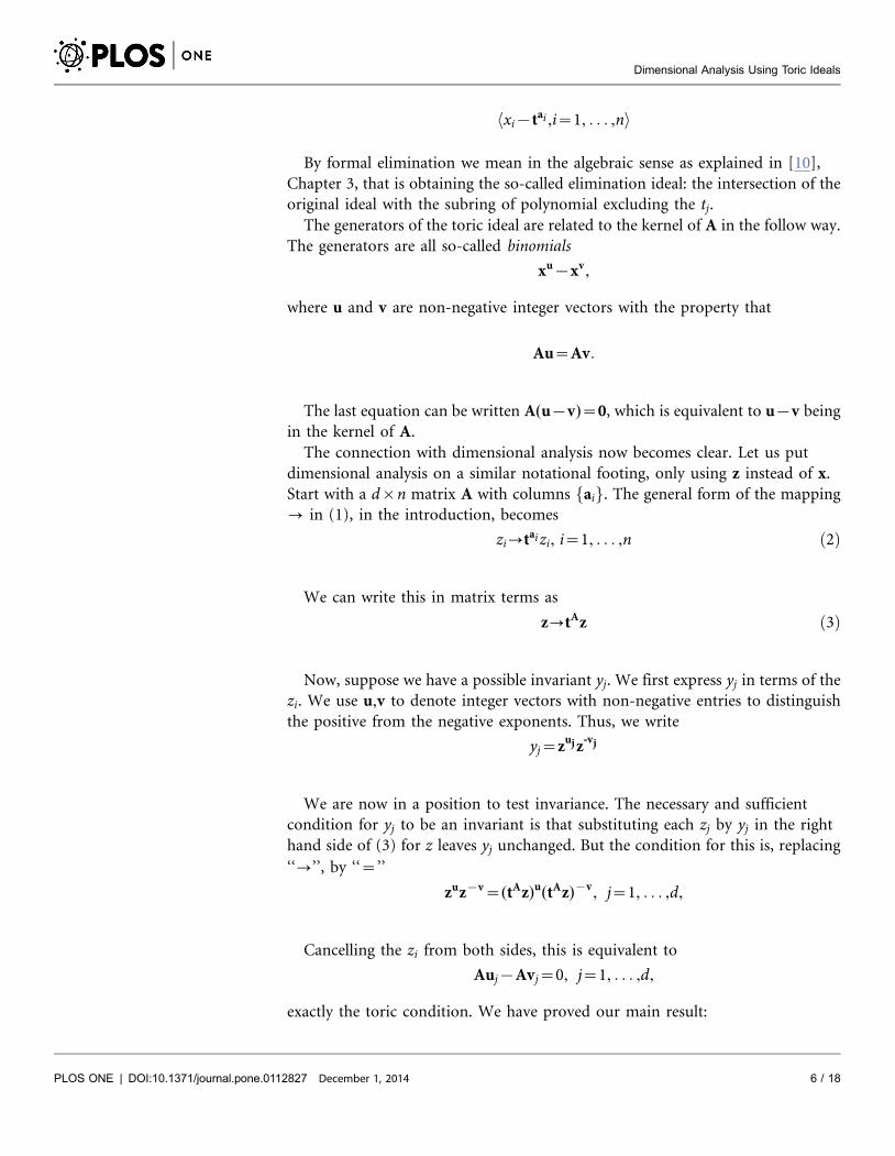
The generators of the toric ideal are related to the kernel of A in the follow way.

The generators are all so-called binomials

xu{xv,

where u and v are non-negative integer vectors with the property that

Au~Av:

The last equation can be written A(u{v)~0, which is equivalent to u{v being

in the kernel of A.

The connection with dimensional analysis now becomes clear. Let us put

dimensional analysis on a similar notational footing, only using z instead of x.

Start with a d|n matrix A with columns faig. The general form of the mapping

? in (1), in the introduction, becomes

zi?taizi, i~1, . . . ,n ð2Þ

We can write this in matrix terms as

z?tAz ð3Þ

Now, suppose we have a possible invariant yj. We first express yj in terms of the

zi. We use u,v to denote integer vectors with non-negative entries to distinguish

the positive from the negative exponents. Thus, we write

yj~zuj z-vj

We are now in a position to test invariance. The necessary and sufficient

condition for yj to be an invariant is that substituting each zj by yj in the right

hand side of (3) for z leaves yj unchanged. But the condition for this is, replacing

‘‘?’’, by ‘‘~’’

zuz{v~(tAz)u(tAz){v, j~1, . . . ,d,

Cancelling the zi from both sides, this is equivalent to

Auj{Avj~0, j~1, . . . ,d,

exactly the toric condition. We have proved our main result:



Theorem 2.1 A variable y~zuj z-vj , for non-negative integer vectors u,v is a

dimensional invariant in a system defined by a matrix A, with derived variable z, if

and only if Au~Av. Moreover the set of all corresponding quantities

zu{zv,

form the toric ideal IA with generator matrix A.

A brief summary is that the set of all dimensionless variables y associated with a

set of quantities defined by an integer matrix A are exactly those given by the toric

ideal IA.

We can give a minimal set of generators for the toric ideal of our running

example. We use the Toric function on the computer algebra package CoCoA, [9],

which takes the matrix A as input. Simply to ease the notation in the use of

computer algebra we use a, . . . ,e, for z1, . . . ,z5. The script with output is.

Use R :: ~QQ½a,b,c,d,e�;Toric([[1,0,0,1,1], [23,1,1,21,1], [0,21,0,21,22]]);

Ideal({d2zae,abc{d,bcd{e)

By the Theorem 2.1, given any generator we have an invariant. Thus {d2zae

yieldsaed2

and we obtain three invariants:

aed2

,abcd

,bcd

e

The second two terms give the dimensional variables from the alternative kernel

matrix K0, above. A key point is that the toric ideal may have more generators

than the rank of the kernel in Buckingham’s theorem. The next section amplifies

this point.

2.1 Saturation and Grobner bases

To summarise, the toric version of dimensional analysis says that we can generate

dimensionless quantities from the toric ideal which is the elimination ideal of the

original power product representation, being careful to use elimination in the

proper algebraic sense.

A lattice ideal associated with an integer defining matrix A is the ideal based on

a full rank kernel matrix. That is if A is d|n with rank d then we find an integer

n|(d{n) matrix K, with rank n{d with rows k1, . . . ,kn{d with AT K~0.

The corresponding lattice ideal is generated by ftkjg. For our first K in

subsection (1) lattice ideal has two generators:

hz1z2z3{z4,z1z22z2

3z24{z5i:

But, as we have seen, this is one fewer generators than the toric ideal. However,

given any such lattice ideal we can obtain the toric ideal using a process called



saturation. The process has two steps. Fix the defining matrix A compute a kernel

K and let IK be a lattice ideal associated with K.

1. Select a dummy variable s and adjoin to the lattice ideal the generator

sPnj~1 xjz1. That is form the sum of the ideals:

IK�~IKzhs Pn

j~1xjz1i:

2. Eliminate s from I�K to give the toric ideal for fx1, . . . ,xng. That is, the toric

ideal is obtained as the elimination ideal for fx1, . . . ,xng.The process of elimination in this saturation process is a formal procedure and

leads to a reduced Grobner basis of the toric ideal which depends in general on the

monomial ordering used in the elimination algorithm. Reduced means all

coefficients of the leading terms are 1 and removing basis terms gives a ring which

cannot contained the remove term; essentially there is no redundancy.

Saturation gives an explanation for the fact that the toric ideal contains, but is

not necessarily equal to the lattice ideal: the addition condition sPnj~1 xjz1~0

giving the variety defined by I�A forces all the xj to be nonzero. Translated into the

original zj the toric ideal description of the dimensionless quantities has the

physical interpretation that it gives the full set of rational polynomial invariants

when none of the defining variables zj is allowed to be zero. This removal of zeros is

intimately connected with the more abstract definitions of toric varieties but we

do not develop this here, see [11].

The Grobner Fan, Primitive Invariants and the Graver Basis

A natural question, given the ease of computing invariants using toric methods, is

whether the invariants obtained in this way are in some sense minimal. This turns

out to be the case. We can illustrate this with our example. A little inspection of

the basis h{d2zae,abc{d,bcd{ei shows that we cannot get simpler invariants

from this basis by multiplication (or division): if

y1~aed2

, y3~bcd

e

then y2~y1y3~abcd

which, although a new invariant, is not obtained by reducing

the numerator or denominator of any of the original invariants.

Definition 1 A basis element zu{zv of IA is called is called primitive if there is no

other (different) basis element invariant zu’{zv’ such that such that zu’ divides zu

and zv’ divides zv. We call an invariant y~zuz{v primitive if and only if zu{zv is

primitive as a basis element of IA.

The following is straightforward alternative definition.



Definition 2 A dimensionless invariant zuz{v is primitive if and only if it cannot

be written as the product of two other such invariants which do not have common

variables.

In the above example y1 and y2 have e in common. In linear programming

notation the condition is that there are no fu0,v0g=fu,vg such that u0ƒu and

v0ƒv, recalling that ‘‘ƒ’’ means entrywise.

Lemma 4.6 of [25] is

Lemma 3.1 Every invariant obtained from a reduced Grobner basis of IA is

primitive.

Note that in what follows we are a little lazy in not to distinguish an invariant

from its inverse.

As mentioned, as we range over all monomial term orderings defining the

individual Grobner basis we obtain the complete Grobner fan and by the Lemma

3.1 and our definition all resulting invariants are primitive. This union of bases is

called the universal Grobner basis and the computer programme Gfan is

recommended to compute the fan [20].

We return to our running example. If we put the G-basis element

h{d2zae,abc{d,bcd{ei into Gfan we obtain the full fan as

hbcd{e,ae{d2,abc{di, he{bcd,abc{di, hd2{ae,bcd{d,abc{di

hd{abc,ab2c2{ei, he{ab2c2,d{abci,

the first of which is the input basis.

The universal Grobner basis of distinct basis terms (ignoring the sign change)

is:

bcd{e,ae{d2,abc{d,ab2c2{e

and we have a new primitive invariant, namely our y2 in the introduction.

Definition 3 The set of all primitive basis elements (which may be larger than the

universal Grobner basis), is called the Graver basis.

Algorithm 7.2 of [25] can be used to compute the Graver basis. The method

starts by constructing from A an extended matrix called the Lawrence lifting:

~A~A 0

I I

� �,

where the zero is a d|n zero matrix and I is a d|d identity matrix. Then

introducing n more derived variables to make a set z1, . . . ,zn,znz1, . . . z2n a toric

ideal is constructed using ~A. Finally, set znz1~ � � �~z2n~1.

The method is conveniently set out in the help screen of ‘‘ToricIdealBasis’’ on

Maple. After inputting



~A~

1 0 0 1 1 0 0 0 0 0

{3 1 1 {1 1 0 0 0 0 0

0 {1 0 {1 {2 0 0 0 0 0

1 0 0 0 0 1 0 0 0 0

0 1 0 0 0 0 1 0 0 0

0 0 1 0 0 0 0 1 0 0

0 0 0 1 0 0 0 0 1 0

0 0 0 0 1 0 0 0 0 1

266666666666664

377777777777775

,

we use the Maple command

zs : ~½seq(z½i�,i~1::10)�;

T : ~ToricIdealBasis(A,zs,plex(op(zs)),method~’hs’,grading~grd);

G : ~subs(½seq(zs½i�~1,i~6::10)�,T);

This yields

hz2z3z4{z5,z1z5{z24,{z4zz1z2z3,{z5zz1z2

2z23i,

In this case the set is the same as given by the fan. That is, the universal Grobner

basis and the Graver basis are the same.

Further Examples

For each of the examples below we give the derived quantities using the classical

notation, (i) the A matrix (ii) a single toric ideal basis given by the default

function on CoCoA and (iii) a full set of primitive basis elements, that is the

Graver basis, given by the maple ToricIdealBasis command and the Lawrence

lifting. From this a full set of primitive invariants is immediate. It turns out that

for all except one of our examples (windmill) the Graver basis is also the universal

Grobner basis. We mention when we find well-known invariants.

;

4.1 Windmill

This standard problem is taken from [15], Section 9.3. (We have changed d there

to D).

It concerns a simple windmill widely used to pump water. The units are: is

shaft power, P ML T2 {3

diameter, D L



;

wind speed, V LT{1

rotational speed, n T{1

air density r ML{3

The A-matrix is

1 0 0 0 1

2 1 1 0 {3

{3 0 {1 {1 0

0B@

1CA

In the a,b . . . notation we obtain, from CoCoA, a basis with 4 terms:

hbd{c,b2c3e{a,c5e{ad2,bc4e{adi

The first entry give a dimensionless quantities discussed in the book:

VnD

:

The universal Grobner basis obtained from the Gfan gives five terms

hbd{c,b2c3e{a,c5e{ad2,bc4e{ad,b5d3e{ai

The last of these is also discussed in the book; it gives the invariant

Prn3d5

:

A full set of 7 primitive invariants, the Graver basis, is

hbd{c,{b2c3eza,a{b3c2de,a{b4cd2e,{b5d3eza,ad{bc4e,ad2{c5ei,

Since rank (A)~3 there are only two algebraically independent invariants. The

standard argument may suggest testing the relationship between any two

independent invariants, for example in a wind tunnel. An important question,

which should be the subject of further research, is say which two or, more

generally, whether the dimensional analysis is sufficiently trusted to test only one

pair and infer other relationships from the algebra.

4.2 Forced convection

The interest is in the following derived quantities: the forced convection

coefficient h, the velocity, u, the characteristic length of the heat transfer surface L,

the conductivity of the fluid k, the dynamic viscosity, m, the fluid specific heat



;

;

;

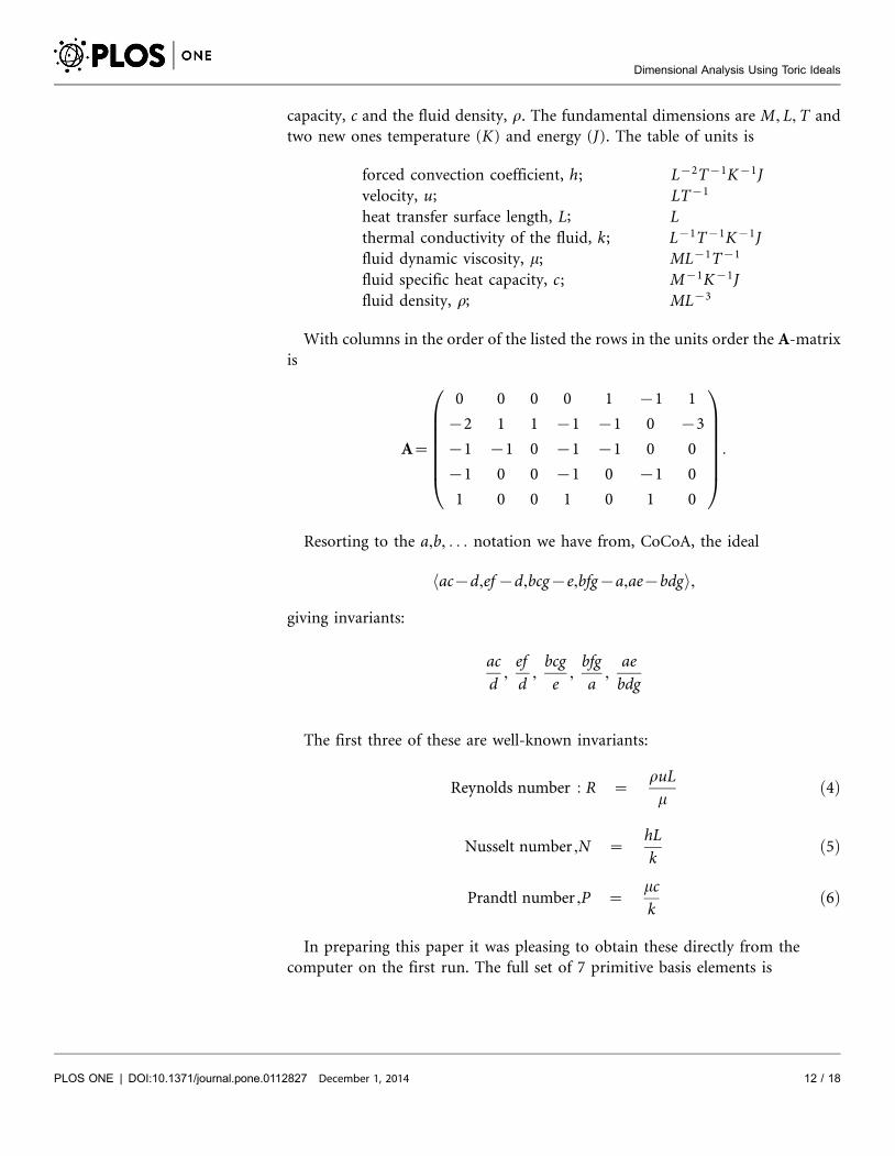
capacity, c and the fluid density, r. The fundamental dimensions are M, L, T and

two new ones temperature (K) and energy (J). The table of units is

forced convection coefficient, h L{2T{1K{1Jvelocity, u LT{1

heat transfer surface length, L Lthermal conductivity of the fluid, k L{1T{1K{1Jfluid dynamic viscosity, m ML{1T{1

fluid specific heat capacity, c M{1K{1Jfluid density, r ML{3

With columns in the order of the listed the rows in the units order the A-matrix

is

A~

0 0 0 0 1 {1 1

{2 1 1 {1 {1 0 {3

{1 {1 0 {1 {1 0 0

{1 0 0 {1 0 {1 0

1 0 0 1 0 1 0

0BBBBBB@

1CCCCCCA:

Resorting to the a,b, . . . notation we have from, CoCoA, the ideal

hac{d,ef {d,bcg{e,bfg{a,ae{bdgi,

giving invariants:

acd

,efd

,bcg

e,

bfga

,ae

bdg

The first three of these are well-known invariants:

Reynolds number : R ~ruL

mð4Þ

Nusselt number ,N ~hLk

ð5Þ

Prandtl number ,P ~mck

ð6Þ

In preparing this paper it was pleasing to obtain these directly from the

computer on the first run. The full set of 7 primitive basis elements is



;

;

;

;

;

;

;

hac{d,ef {d,bcg{e,bfg{a,ae{bdg,bcfg{d,ac{ef i

The simplest of the ‘‘new’’ primitive invariants is from ac{ef :

hLmc

,

which is the Reynolds number divided by the Nusselt number.

4.3 Electrodynamics

As an exercise we take six basic quantities for electro-dynamics and use the

literature to give some expression in terms of mass (M), length (L), time (T) and

current (A). We do not have any particular electromagnetic device in mind, but

simply try to find some dimensionless quantities. The following is one version:

charge TApotential ML2T{3A{1

capacitance M{1L{2T4A2

inductance ML2T{2A{2

resistance ML2T{3A{2

Then

A~

0 1 {1 1 1

0 2 {2 2 2

1 {3 4 {2 {3

1 {1 2 {2 {2

0BBB@

1CCCA:

CoCoA gives

hbc{a,{ce2zd,{ae2zbdi:

Note that A only has rank 3. It turns out that this is a complete list of primitive

basis elements.

4.4 Hydrogen atom

Toric ideals are embedded in advanced models in physics but one can get some

way with simple dimensional analysis. This example is given in some form by a

number of authors. We found [24], section 1.3.1, useful. The hydrogen atom

consists of a proton and a neutron and the Bohr radius is the distance between

them. We have used slightly non-standard notation. In a somewhat cavalier

manner we have introduced the speed of light as a derived quantity.



mass of electron, me MBohr radius, a0 Lenergy, E ML{2T{2

Plank’s constant, B ML2T{1

e2 (e is elementary charge) ML3T{2

speed of light, c LT{1

Then

A~

1 0 1 1 1 0

0 1 2 2 3 1

0 0 {2 {1 {2 {1

0B@

1CA

The ideal is

h{df ze,bc{df ,abe{d2,{cd2zae2,abf {d,af 2{c,aef {cdi:

(The algebraic e is e2 and the algebraic c should not be confused with the speed

of light). The first terms gives an invariant called the ‘‘fine structure constant’’

e2

Bc:

If we take the third term and interpretx2

uvybeing invariant as stating that

v~constant|x2

uy, then we have a well known formula for a0 interpreted as the

size of the hydrogen atom:

a0~constant|B2

mee2:

We cannot resist stating that the sixth basis element, af 2{c gives

E~constant|mec2:

The Graver basis gives a set of 10 primitive invariants for the hydrogen atom:

hdf {e,bc{e,bc{df ,af 2{c,{cdzaef ,

{cd2zae2,abf {d,abf 2{e,abe{d2,{d2zab2ci:

It is not known whether this list has been given explicitly before.



;

;

;

;

;

;

The Wider Picture: Group Invariance

Dimensional analysis should be considered as a special case of the theory of group

invariance and in an attempt to suggest a natural generalisation we very briefly

sketch the theory of invariants.

We start with the action of a Lie group G acting on a manifold M in Rd. The

manifold will be our model and the group something to do with our physical

understanding. The orbit of O(x) for a point x in M be the set of all g(x) for all g in

G. If M is invariant under G then O(x)5M. This sets up an equivalence relation

with members of M in which the same orbit are equivalent. The collection of

equivalence classes is denoted by the quotient M=G and the projection

p : M?M=G maps every member of of M into its correct equivalence class.

Under suitable conditions M=G is a manifold in its own right and we say that Gacts regularly on M. Also, the mapping p can be used to set up a coordinate system

on M=G and note that p itself is an invariant. This discussion leads naturally to

the following.

Proposition 5.1 Let a group G act regularly on a manifold M. A manifold defined

by a smooth function F is a set SF~fxjF(x)~0. It is G-invariant if and only if there

is a function F� defining a smooth sub-manifold SF�~fyjF�(y)~0g on M=G such

that

SF�~p(SF),

where p is the projection from M to M=G.

A one parameter Lie group G shifts a point x along an integral curve Y(E,x) by a

flow. If we expand Y(E,x) in a Taylor expansion in E we obtain:

Y(E,x)~xzEj(x)zO(E2):

The term j(x)~(j1(x), . . . ,jd(x)) defines a vector field and we can write v in

classical local coordinates:

v~j1(x)L

Lx1z � � �zjd(x)

LLxd

A function y is an invariant if v:y~0, namely

j1(x)Ly

Lx1z � � �zjd(x)

Ly

Lxd~0:

This is a first order partial differential equation which can be solved by first

writing down

dx1

j1(x)~ � � �~ dxd

jd(x),

namely by the methods of characteristics. The solutions take the form:



y1(x)~c1, � � � ,ym(x)~cm,

where the yj are the invariants.

In our notation E becomes t and using our generating matrix A the mapping ?in (3) is

Y(t,z)~tAz:

Performing matrix partial differentiation with respect to t, and setting all ti~1gives the infinitesmal generators:

v~ALLz:

An interpretation of the toric variety is as characterising the orbits of the scale

group of transformation, as discussed above. We have not formally proved the

Buckingham theorem, but drawing on the above discussion it is given as Theorem

2.22 in [23].

Limitations of the Study, Open Questions and Future Work

We have seen that the toric ideal method, via the Graver basis, is a fast way to

compute all primitive invariants in dimensional analysis. There are some areas of

further study which this suggests.

The first area arises from the possibility that different physical systems may

yield different types of toric ideal or variety. The most important general class is

normal toric varieties. Briefly, such varieties are related to polyhedral cones and

polyhedra with integer or rational generators. The standard approach is to take

the a suitable cone s and compute its Hilbert basis, which is a set of integer

generators of the dual cone giving all integer grid points in that cone. From this

there is a natural toric ideal. But an open problem, it seems to the authors, is

whether this rich theory of normal varieties and polyhedra has a role in classical

physics and engineering.

A second area is a natural development from the previous section. A discussion

missing from this paper is the way in which differentials are converted to derived

quantities. For example velocity, which isLyLt

, for some length variable y and time t

is allocated the units LT{1. One way to keep the advantages of awarding derived

quantities to differential terms, but retain differentials is to use combinations of

differential and polynomial operators. The algebraic environment which allows

this is differential algebra and in particular Weyl algebras. Much of the existing

work uses the methods to study identifiability (see [22]) but the challenge, here, is

to find differential-algebraic invariants in the same spirit as the invariants in this



paper. A noteworthy development is [17–19], especially in the context of

dynamical systems.

Finally, the authors are aware of the value of standard dimensional analysis

when the exponents are rational but not necessarily integer. This arises in the

work on turbulence mentioned [7, 8]. This can be studied by changing the base

lattice to have fractional levels and the authors are considering research in this

area.

Conclusions

Toric ideals are the appropriate framework for dimensional analysis with describe

the rational invariants under the multivariate scale group. The key contribution is

that the Graver basis, which can be the thought of as a unique ‘‘envelope’’ of bases

for the toric ideal and consists of all primitive elements then gives rise to a notion

of primitive invariants. These comprise the invariants which cannot be split into

the product of two other invariants using disjoint sets of units. The suggestion is

that this solves a classical but sometimes unspoken conundrum in dimensional

analysis: namely that invariants produced by the celebrated Buckingham method

are not unique. In addition the Graver basis is easily computed using computer

algebra. In some examples we are able to find some named invariants, all,

satisfyingly, primitive. But also, because the Graver basis is larger than a minimal

basis for the toric ideal the methods throws up new primitive invariants which

may attract scientific interest.

Acknowledgments

Many computations in this paper were performed by using Maple a trademark of

Waterloo Maple Inc.

Author ContributionsWrote the paper: HPW. Supplied most of the engineering/physics input including

ellucidation and interpretation of example: MA. Computational work on Grobner

base, Engineering design motivation: RB.

References

1. Albrecht MC, Nachtsheim CJ, Albrecht TA, Cook RD (2013) Experimental design for engineeringdimensional analysis. Techometrics 55: 257–270.

2. Barnett W (2007) Dimensions and economics: some problems. Quarterly J. Austrian Economics 1: 95–104.

3. Bhaskar R, Nigan A (1990) Qualitative physics using dimensional analysis. Artificial Intelligence 45: 73–111.

4. Buckingham E (1919) On physically similar systems: illustration of the use of dimensional analysis.Physics Review 4: 345–376.



5. Buckingham E (1915) The principle of similitude. Nature 96: 396–397.

6. Buckingham E (1915) Model experiments and the forms of empirical equations. Trans. Amer. Soc.Mech. Eng. 37: 263–296.

7. Chapman SC, Watkins NW (2009) Avalanching systems under intermediate driving rate. Plasma Phys.Control Fusion 51: (124006).

8. Chapman SC, Rowlands G, Watkins NW (2009) Macroscopic control parameter for avalanche modelsof bursty transport. Physics of Plasmas 16: (012303)

9. CoCoA: a system for doing Computations in Commutative Algebra. Available: http://cocoa.dima.unige.it

10. Cox DA, Little JB, O’Shea D (2007) Ideals, varieties, and algorithms: an introduction to computationalalgebraic geometry and commutative algebra. Third Edition. Springer, New York. 553 p.

11. Cox DA, Little JB, Schenck HK (2011) Toric varieties. Graduate Studies in Mathematics: 124. AmericanMathematical Society, Providence, Rhode Island. 841 p.

12. D’Agostino S (2002) A history of the ideas of theoretical physics. Kluwer, Dordrecht. 381 p.

13. Davis T (2013) Comment: dimensional analysis in statistical engineering. Technometrics 55: 271–274.

14. Gibbings JC (1986) The systematic experiment. Cambridge University Press, Cambridge. 352 p.

15. Gibbings JC (2011) Dimensional analysis. Springer, London. 312 p.

16. Grove DM, Davis TP (1992) Engineering, quality and experimental design. Longmans, London. 361 p.

17. Hubert E, Labahn G (2013) Scaling Invariants and Symmetry Reduction of Dynamical Systems.Foundations Computational Mathematics 13: 479–516.

18. Hubert E, Kogan I (2007) Rational Invariants of a Group Action. Construction and Rewriting. Journal ofSymbolic Computation, 42: 203–217.

19. Hubert E (2013) Rational Invariants of a Group Action. Journees Nationales de Calcul Formel 3:(hal.inria.fr/hal-00839283)

20. Jensen AN (2011) Gfan, a software system for Grobner fans and tropical varieties. http://home.imf.au.dk/jensen/software/gfan/gfan.html.

21. Bolster D, Hershberger RE, Donelly RJ (2011) Dynamic similarity, the dimensionless science.Physices today. 64:(9) 42–47.

22. Margaria G, Riccomagno E, Chappell MJ, Wynn HP (2001) Differential algebra methods for the studyof the structural identifiability of rational function state-space models in the biosciences. MathematicalBiosciences 174: 1–26.

23. Olver PJ (1986) Application of Lie groups to differential equations. Springer, New York. 513 p.

24. Smith H (1991) An introduction to quantum mechanics. World Scientific, New York. 285 p.

25. Sturmfels B (1996) Grobner Bases and convex polytopes. University Lecture Note Series: 8 Amer.Math. Soc, Providence, Rhode Island. 162 p.

26. Szirtes T (2007) Applied Dimensional Analysis and Modeling. Butterworth-Heinemann, Burlington. 820p.



http://cocoa.dima.unige.it

http://home.imf.au.dk/jensen/software/gfan/gfan.html

http://home.imf.au.dk/jensen/software/gfan/gfan.html

Dimensional Analysis Using Toric Ideals: Primitive Invariants

Documents

Transcript of Dimensional Analysis Using Toric Ideals: Primitive Invariants