Hall invariants, homology of subgroups, and characteristic varieties

arX

iv:m

ath/

0010

046v

1 [

mat

h.G

R]

4 O

ct 2

000

HALL INVARIANTS, HOMOLOGY OF SUBGROUPS,

AND CHARACTERISTIC VARIETIES

DANIEL MATEI AND ALEXANDER I. SUCIU

Abstract. Given a finitely-generated group G, and a finite group Γ, Philip Halldefined δΓ(G) to be the number of factor groups of G that are isomorphic to Γ.We show how to compute the Hall invariants by cohomological and combinato-rial methods, when G is finitely-presented, and Γ belongs to a certain class ofmetabelian groups. Key to this approach is the stratification of the charactervariety, Hom(G, K∗), by the jumping loci of the cohomology of G, with coeffi-cients in rank 1 local systems over a suitably chosen field K. Counting relevanttorsion points on these “characteristic” subvarieties gives δΓ(G). In the process,we compute the distribution of prime-index, normal subgroups K ⊳ G accordingto dimK H1(K; K), provided char K 6= |G : K|. In turn, we use this distributionto count low-index subgroups of G. We illustrate these techniques in the casewhen G is the fundamental group of the complement of an arrangement of eitheraffine lines in C2, or transverse planes in R4.

Contents

1. Introduction 22. Eulerian functions and Hall invariants 53. Counting abelian representations 84. Homology of finite-index subgroups 95. Alexander matrices and characteristic varieties 146. Torsion points and Betti numbers 167. Counting metabelian representations 198. Counting finite-index subgroups 229. Arrangements of complex hyperplanes 2610. Arrangements of transverse planes in R4 28References 32

2000 Mathematics Subject Classification. Primary 20J05, 57M05; Secondary 20E07, 52C35.Key words and phrases. Hall invariant, Eulerian function, finite-index subgroup, homology,

Alexander matrix, characteristic variety, torsion point, arrangement.Research partially supported by an RSDF grant from Northeastern University.

1

http://arXiv.org/abs/math/0010046v1

2 DANIEL MATEI AND ALEXANDER I. SUCIU

1. Introduction

1.1. Hall invariants. In [18], Philip Hall introduced several notions in group the-ory. Given a finitely-generated group G, and a finite group Γ, he defined δΓ(G) tobe the number of surjective representations of G to Γ, up to automorphisms of Γ:

δΓ(G) = |Epi(G,Γ)/AutΓ| .(1.1)

In other words, the Hall invariant δΓ(G) counts all factor groups of G that areisomorphic to Γ. When G = π1(X) is the fundamental group of a connected 2-complex X with finite 1-skeleton, δΓ(π1(X)) counts all connected, regular covers ofX with deck transformation group Γ.

Suppose G has a finite presentation, with generators x1, . . . , xn, and relatorsr1, . . . , rm. The Hall invariant δΓ(G) can be computed by counting generating setsof Γ that have size n and satisfy the relations rj in Γ, and then dividing the result bythe order of Aut(Γ). While this method can be implemented on a computer algebrasystem like GAP [15]1, the computation breaks down even for moderately large nand |Γ|. One of the purposes of this paper is to show how the Hall invariants δΓ(G)can be computed more efficiently, by combinatorial and homological methods, atleast when Γ belongs to a certain class of finite metabelian groups.

1.2. Abelian representations. In Section 2, we start by recalling a formula ofHall [18]. Using what he called the Eulerian function of the finite group Γ, togetherwith Mobius inversion, Hall showed that δΓ(G) = 1

|AutΓ|

∑H≤Γ µ(H) |Hom(G,H)|,

where µ is the Mobius function of the subgroup lattice of Γ. For a p-group Γ, theMobius and Eulerian functions were computed by Weisner [43].

In Section 3, we use these results of Hall and Weisner, together with a result fromMacdonald’s book [30], to arrive at a completely explicit formula for δΓ(G) in thesimplest case: that of a finite abelian group Γ. The expression for δΓ(G), given inTheorem 3.1, depends only on Γ and the abelian factors of G. A similar expressionwas obtained (by other means) in [22], in the particular case G = Fn.

1.3. Metabelian representations. The next level of difficulty in computing Γ-Hall invariants is presented by (split) metabelian groups Γ. Suppose Γ = B ⋊σ Cis a semidirect product of abelian groups, with monodromy homomorphism σ :C → Aut(B). An epimorphism λ : G ։ Γ may be thought of as the lift of anepimorphism ρ : G ։ C. As explained in [28], the lifts of a fixed homomorphismρ : G → C are parametrized by H1(G,Bρ), the first cohomology group of G withcoefficients in the G-module B = Bρ, with action g · b = σ(ρ(g))(b).

1The GAP command that computes δΓ(G) is GQuotients(G,Γ). We were led to consider theHall invariants after reading about this command in the GAP manual.

HALL INVARIANTS AND CHARACTERISTIC VARIETIES 3

We consider split metabelian groups Γ = B ⋊σ C for which B is an elementaryabelian group, and C is a finite cyclic group. If K is a finite field with additivegroup B, then H1(G,Bρ) may be identified with H1(G,Kρ) where again G acts onK by means of ρ. Now Shapiro’s Lemma identifies the twisted cohomology groupH1(G,Kρ) with the untwisted cohomology group H1(Kρ,K), where Kρ = ker ρ. Weare thus led to investigate the homology of finite-index, normal subgroups of G.

1.4. Homology of finite-index subgroups. Let G be a finitely-presented group,and K ⊳ G a normal subgroup. Assume the quotient group, Γ = G/K, is finite. Aprocedure to compute H1(K,Z) from a presentation of G and the coset representa-tion of G on G/K was given by Fox [13]. The efficiency of Fox’s method decreasesrapidly with the increase in the index |Γ| = |G : K|. In Section 4, we overcome thisproblem, at least partially. Our approach (similar to that of Hempel [19, 20] andSakuma [39]) is based on the representation theory of Γ, over suitably chosen fieldsK.

Consider the homology group H1(K,K), and set b(q)1 (K) := dimK H1(K,K),

where q = char K. The idea is to break H1(K,K) into a direct sum, accordingto the decomposition of the group algebra KΓ into irreducible representations. Inorder for this to work, we need the field K to be “sufficiently large” with respectto Γ; that is, q should not to divide |Γ|, and K should contain all roots of unity oforder equal to the exponent of Γ. Let λ : G ։ Γ be an epimorphism, with kernelK = Kλ. In Theorem 4.6, we prove:

b(q)1 (Kλ) = b

(q)1 (G) +

∑

ρ6=1

nρ(corank Jρλ − nρ),(1.2)

where ρ runs through all non-trivial, irreducible representations of Γ over the fieldK, and Jρλ is the Jacobian matrix of Fox derivatives of the relators, J = JG,followed by the representation ρ λ : G→ GL(nρ,K).

When Γ is abelian and K = C, we recover from (1.2) a well-known result ofLibgober [23] and Sakuma [39]: b1(Kλ) = b1(G) +

∑ρ6=1

(corank Jρλ − 1), where ρruns through all non-trivial, irreducible, complex representations of Γ. For otherchoices of K, formula (1.2) gives information about the q-torsion coefficients ofH1(K,Z), provided q ∤ |Γ|.

1.5. Torsion points on characteristic varieties. The next step is to interpretformula (1.2) in terms of the “Alexander stratification” of the character variety ofG. This can be done for an arbitrary finite abelian group Γ, but, for simplicity, werestrict our attention to the case when Γ is cyclic, which is enough for our purposeshere.

In Section 5, we start by reviewing the pertinent material on Alexander idealsand their associated varieties, in a more general context than usual. The Alexander


matrix, AG, is the abelianization of the Fox Jacobian, JG. The d-th characteristicvariety, Vd(G,K), is the subvariety of Hom(G,K∗) defined by the codimension dminors of AG. It can be shown that Vd(G,K)\1 is the set of non-trivial characterst ∈ Hom(G,K∗) for which dimK H

1(G,Kt) ≥ d, see [21] and Remark 5.4.In Section 6, we study the relationship between torsion points on the character-

istic varieties of G and the homology of finite-index, normal subgroups K ⊳ G. Asmentioned above, we only consider the case when Γ = G/K is cyclic, say Γ = ZN .In Theorem 6.2, we prove:

b(q)1 (Kλ) = b

(q)1 (G) +

∑

16=k|N

φ(k)dK(λN/k).(1.3)

where dK(t) = max d | t ∈ Vd(G,K) is the depth of the character t ∈ Hom(G,K∗)with respect to the Alexander stratification. In particular, if N = p is prime, then:

b(q)1 (Kλ) = b

(q)1 (G) + (p− 1)dK(λ).(1.4)

In view of (1.4), we define β(q)p,d(G) to be the number of index p, normal subgroups

K ⊳ G for which b(q)1 (K) = b

(q)1 (G) + (p− 1)d. In Theorem 6.5, we prove:

β(q)p,d(G) = 1

p−1|Torsp,d(G,K) \ Torsp,d+1(G,K)| ,(1.5)

where K = C if q = 0, and K = Fqs (s = order of q in F∗p) if q 6= 0, and Torsp,d(G,K)

is the set of characters in Vd(G,K) of order exactly p.

1.6. Metabelian Hall invariants and low-index subgroups. Once this is done,we are ready to return to the Hall invariants of G. In Section 7, we compute δΓ(G),for split metabelian groups Γ of the form Mp,qs = Zs

q ⋊σ Zp, where p and q aredistinct primes, s = ordp(q), and σ has order exactly p. Examples are the dihedralgroups D2p = M2,p and the alternating group A4 = M3,4. In Theorem 7.7, we prove:

δMp,qs (G) = p−1s(qs−1)

∑

d≥1

β(q)p,d(G)(qsd − 1).(1.6)

This generalizes a result of Fox [14], who was the first to use Alexander matricesfor counting metacyclic representations of fundamental groups of knots and links.Put together, formulas (1.6) and (1.5) express the Hall invariant δMp,qs (G) in termsof the number of p-torsion points on the Alexander strata of the character varietyHom(G,Fqs).

In Section 8, we use formula (1.6), together with several formulas from §§2–3,to derive information about the number, ak(G), of index k subgroups of G. It wasMarshall Hall [17] who showed how to compute these numbers recursively, in terms


of |Hom(G, Sl)|, 1 ≤ l ≤ k. Applying this method, we obtain (in Theorem 8.2):

a3(G) = 12(3n − 1) + 3

2

∑

d≥1

β(3)2,d(G)(3d − 1),(1.7)

where n = b(3)1 (G). We also give formulas of this sort for the number, a⊳k(G), of

index k, normal subgroups of G, provided k ≤ 15 and k 6= 8 or 12.

1.7. Arrangement groups. We conclude with some explicit examples and com-putations in the case when G is the fundamental group of the complement of asubspace arrangement. This is meant to illustrate the theory developed so far, ina setting where topology and combinatorics are closely intertwined.

In Section 9, we look at complex hyperplane arrangements. By the Lefschetz-type theorem of Hamm and Le, it is enough to consider arrangements of affinelines in C2. If G is the group of such an arrangement, the characteristic varietiesVd(G,C) are well understood: they consist of subtori of the character torus, pos-sibly translated by roots of unity. Furthermore, the tangent cone at the origin toVd(G,C) coincides with the “resonance” variety Rd(G,C), which is determined bythe combinatorics of the arrangement. The components of Vd(G,C) not passingthrough the origin, though, are not a priori combinatorially determined. Theirappearance affects the torsion coefficients in the homology of certain finite abeliancovers of the complement, as we show in Example 9.3.

In Section 10, we turn to real arrangements. More precisely, we consider arrange-ments of transverse planes through the origin of R4. If G is the group of such a2-arrangement, the varieties Vd(G,C) need not be unions of translated subtori, asshown in [32], and also here, in Example 10.3. Furthermore, the tangent cone atthe origin to Vd(G,C) may not coincide with the resonance variety Rd(G,C), as wepoint out in Remark 10.4. Finally, using the metabelian Hall invariants δS3 andδA4 , we recover the homotopy-type classification of complements of 2-arrangementsof n ≤ 6 planes in R4 (first established in [32]), and extend it to horizontal arrange-ments of n = 7 planes.

Acknowledgment. The computations for this work were done with the help ofthe packages GAP 4.1 [15], Macaulay 2 [16], and Mathematica 4.0.

2. Eulerian functions and Hall invariants

We start by reviewing two basic notions introduced by Philip Hall in [18]: theEulerian function, φ(Γ, n), of a finite group Γ, and the Hall invariants, δΓ(G), of afinitely-generated group G.


2.1. Eulerian function. Let Γ be a finite group. The Eulerian function of Γ isdefined as

φ(Γ, n) = #ordered n-tuples (g1, . . . , gn) that generate Γ,(2.1)

where repetitions among the gi’s are allowed. For example, φ(Zk, 1) = φ(k), theusual Euler totient function.

Let L(Γ) be the lattice of subgroups of Γ, ordered by inclusion. Let µ : L(Γ) → Zbe the Mobius function, defined inductively by µ(Γ) = 1,

∑H≤K µ(H) = 0. Then,

the Eulerian function of Γ is given by:

φ(Γ, n) =∑

H≤Γ

µ(H) |H|n ,(2.2)

see [18], and also [5] for a recent account.The Eulerian function and the Mobius function of a finite p-group were computed

by Weisner in [43]. To formulate Weisner’s results, recall that the Frattini subgroupof a finite group Γ, denoted Frat Γ, is the intersection of all maximal, proper sub-groups of Γ. If Γ is a p-group, then FratΓ = [Γ,Γ] · Γp, by the Burnside BasisTheorem (cf. [37, p. 140]).

According to Weisner, the Mobius function of a finite p-group Γ is given by:

µ(H) =

(−1)dp

d(d−1)2 , where pd = |Γ : H| if FratΓ ≤ H,

0 if FratΓ 6≤ H.(2.3)

Now set pr = |Γ| and ps = |Γ : Frat Γ|. The Eulerian function of Γ is then given by:

φ(Γ, n) = p(r−s)ns−1∏

i=0

(pn − pi).(2.4)

2.2. Hall invariants. Let G be a finitely-generated group, and Γ a finite group.Let σΓ(G) = |Hom(G,Γ)| be the number of homomorphisms G→ Γ, and φΓ(G) =|Epi(G,Γ)| the number of epimorphisms G ։ Γ. The relation between σ and φ isgiven by Hall’s enumeration principle:

σΓ(G) =∑

H≤Γ

φH(G),(2.5)

or, by Mobius inversion:

φΓ(G) =∑

H≤Γ

µ(H)σH(G).(2.6)

Definition 2.3. Let G be a finitely-generated group. Let Γ be a finite group, withautomorphism group Aut Γ. The Γ-Hall invariant of G is δΓ(G) = φΓ(G)/ |Aut Γ|.


1ONMLHIJKMp,q

−1 GFED@ABCZqkkkkkkkkkkkkk

q 765401231<<

<<<<

<<<<

<<<<

<<<<

<<<

−1GFED@ABCZp

----

----

--

−1. . .

︸︷︷︸q

GFED@ABCZp

−1GFED@ABCZp

<<<<

<<<<

<<<<

1GFED@ABCA4

−1 GFED@ABCZ22

0

GFED@ABCZ2

4 765401231CC

CCCC

CCCC

C0

GFED@ABCZ2

1111

1111 0

GFED@ABCZ2

1111

111

−1

GFED@ABCZ3

1111

111

−1

GFED@ABCZ3

CCCC

CCCC

CCC

−1

GFED@ABCZ3

LLLLLLLLLLLLLLL

−1

GFED@ABCZ3

QQQQQQQQQQQQQQQQQQQQ

ttttttttttttttttttttttt

Figure 1. The subgroup lattice and Mobius function of Mp,q and A4

Since Aut Γ acts freely and transitively on Epi(G,Γ), the number δΓ(G) is aninteger, which counts epimorphisms G ։ Γ, up to automorphisms of Γ. In otherwords, δΓ(G) is the number of homomorphs of G that are isomorphic to Γ.

Note that

φΓ1×Γ2(G) = φΓ1(G)φΓ2(G)(2.7)

whenever Γ1 and Γ2 are finite groups, with (|Γ1| , |Γ2|) = 1. In that situation, wealso have Aut(Γ1 × Γ2) = Aut(Γ1) × Aut(Γ2), and so δΓ1×Γ2(G) = δΓ1(G)δΓ2(G).

Now let G = Fn, the free group of rank n. Clearly, σΓ(Fn) = |Γ|n and φΓ(Fn) =φ(Γ, n). Hence, by (2.2):

δΓ(Fn) =

∑H≤Γ µ(H) |H|n

|Aut(Γ)|.(2.8)

Example 2.4. Let Mp,q = Zq⋊Zp be the metacyclic group of order pq, where p andq are primes, with p | (q−1). Its subgroup lattice and Mobius function are shown inFigure 1. The automorphism group of Mp,q is isomorphic to Mq−1,q

∼= Zq⋊Aut(Zq),the holomorph of Zq. By (2.8):

δMp,q(Fn) =

(pn − 1)(qn−1 − 1)

q − 1.(2.9)

Example 2.5. Let A4 be the alternating group on 4 symbols. The Mobius functionis given in Figure 1. Furthermore, Aut(A4) ∼= S4, the symmetric group on 4symbols. We get:

δA4(Fn) =(3n − 1)(4n−1 − 1)

6.(2.10)


3. Counting abelian representations

In this section, we show how to compute the Hall invariant δΓ(G), in case Γ isa finite abelian group. We start with the well-known computation of the order ofAut(Γ).

For a prime p, denote by Γp the p-torsion part of Γ. Then Γ =⊕

p||Γ| Γp, and

|Aut(Γ)| =∏

p| |Γ|

|Aut(Γp)| .(3.1)

Let A be a (finite) abelian p-group. Then A = Zpπ1 ⊕· · ·⊕Zpπr , for some positiveintegers π1 ≥ · · · ≥ πr, and so A determines (and is determined by) a partitionπ(A) = (π1, . . . , πr). Given such a partition π, let l(π) = r be its length, and|π| =

∑ri=1 πi its weight. Also, let 〈π〉 =

∑ri=1(i− 1)πi. Then:

|Aut(Zpπ1 ⊕ · · · ⊕ Zpπr )| = p|π|+2〈π〉∏

k≥1

ϕmk(π)(p−1),(3.2)

where mk(π) = #j | πj = k is the multiplicity of k in λ, and ϕm(t) =∏m

i=1(1−ti);

see Macdonald [30, p. 181]2.Given a partition λ, let λ′ be the partition with λ′i = λi − 1. If τ is another par-

tition, let θi(λ, τ) =∑l(τ)

j=1 min(λi, τj), for 1 ≤ i ≤ l(λ), and θ(λ, τ) =∑l(λ)

i=1 θi(λ, τ).With these notations, we have the following:

Theorem 3.1. Let G be a finitely-generated group and Γ a finite abelian group.Write H1(G) = Zn ⊕ T , where T is finite. For each prime p dividing |Γ|, letλ = π(Γp) and τ = π(Tp) be the corresponding partitions. Then:

δΓ(G) =∏

p| |Γ|

p(|λ|−l(λ))n+θ(λ′,τ)∏l(λ)

i=1(pn+θi(λ,τ)−θi(λ

′,τ) − pi−1)

p|λ|+2〈λ〉∏

k≥1 ϕmk(λ)(p−1).(3.3)

Proof. Since Γ is abelian, every homomorphism G → Γ factors through H1(G) =Zn ⊕ T . By (2.7), we have φΓ(G) =

∏p| |Γ| φΓp

(Zn ⊕ T ). Furthermore, everyhomomorphism Zn ⊕ T → Γp factors through Zn ⊕ Tp. Hence:

φΓ(G) =∏

p| |Γ|

φΓp(Zn ⊕ Tp).(3.4)

By Hall’s enumeration principle (2.6), we have:

φΓp(Zn ⊕ Tp) =

∑

H≤Γp

µ(H)σH(Zn ⊕ Tp).(3.5)

2We are grateful to A. Zelevinsky for pointing this reference to us.


Clearly, σH(Zn ⊕ Tp) = |H|n pθ(ν,τ), where ν = π(H). The Mobius function of asubgroup H of Γp can be computed from Weisner’s formula (2.3), as follows.

Let Frat Γp be the Frattini subgroup of Γp. Then Frat Γp = (Γp)p, and so the

associated partition is λ′, where λ = π(Γp) and λ′i = λi − 1. If a subgroup H of Γpdoes not contain Frat Γp, then µ(H) = 0. If H contains FratΓp, then the partitionν = π(H) is between λ′ and λ, i.e., νj = λj−1 or λj . Order the set j | νj = λj−1as (i1 ≥ · · · ≥ id). Clearly, pd = |Γ : H|, and so µ(H) = (−1)dpd(d−1)/2.

The number of subgroups H ≤ Γp such that Frat Γp ≤ H and π(H) = ν equals

pa, where a =∑d

k=1(ik − k). Set dν = d and aν = a. A simple calculation nowshows:

φΓp(Zn ⊕ Tp) =

∑

Frat Γp≤H≤Γp

µ(H)σH(Zn ⊕ Tp)

=∑

λ′νλ

(−1)dνpdν(dν−1)/2p(|λ|−dν)npθ(ν,τ)paν

= p(|λ|−l(λ))n+θ(λ′,τ)∏

i≥1

(pn+θi(λ,τ)−θi(λ′,τ) − pi−1).

This, together with formulas (3.1), (3.2), and (3.4), yields (3.3).

Especially simple is the case when the group G has torsion-free abelianization.

Corollary 3.2. Let G be a finitely generated group with H1(G) = Zn, and Γ afinite abelian group. Write Γ =

∏p| |Γ|

Γp, where Γp = Zpλ1 ⊕ · · · ⊕ Zpλr . Then

δΓ(G) =∏

p| |Γ|

p|λ|(n−1)−2〈λ〉ϕn(p−1)

ϕn−r(p−1)∏

k≥1 ϕmk(λ)(p−1).(3.6)

A formula similar to (3.6) was obtained by Kwak, Chun, and Lee [22, Theorem3.4]. In particular (writing Zs

p for the direct sum of s copies of Zp):

δZps (G) = psn−p(s−1)n

ps−ps−1 , δZsp(G) =

s−1∏

i=0

pn−pi

ps−pi , δZp⊕Zps (G) = (psn−p(s−1)n)(pn−p)ps+1(p−1)2

.

4. Homology of finite-index subgroups

In this section, we give a formula for computing the first homology (with coeffi-cients in a “sufficiently large” field) of finite-index, normal subgroups of a finitely-presented group.


4.1. Fox calculus. Let G = 〈x1, . . . , xℓ | r1, . . . , rm〉 be a finite presentation forthe group G. Let Fℓ be the free group with generators x1, . . . , xℓ, and φ : Fℓ → Gthe presenting epimorphism. Let ZFℓ be the group-ring of Fℓ, and ǫ : ZFℓ → Z theaugmentation map. For each 1 ≤ j ≤ ℓ, there is a Fox derivative, ∂

∂xj: ZFℓ → ZFℓ,

which is the linear operator defined by the rules ∂1∂xj

= 0, ∂xi

∂xj= δij , and ∂(uv)

∂xj=

∂u∂xjǫ(v) + u ∂v

∂xj.

Let X be the 2-complex associated with the presentation G = 〈x1, . . . , xℓ |

r1, . . . , rm〉. Let X be the universal cover, and C∗(X) its augmented cellular chaincomplex. Picking as generators for the chain groups the lifts of the cells of X, the

complex C∗(X) becomes identified with

(ZG)mJG−→ (ZG)ℓ

∂1−→ ZGǫ−→Z → 0,(4.1)

where ∂1 =(x1 − 1 · · · xℓ − 1

)⊤

, and

JG =(∂ri∂xj

)φ

is the Jacobian matrix of G, obtained by applying the linear extension φ : ZFℓ →ZG to the Fox derivatives of the relators.

Clearly, the integral m× ℓ matrix J ǫG is a presentation matrix for H1(G). Moregenerally, the abelianization of a finite-index subgroup K ≤ G is given by thefollowing result of Fox.

Theorem 4.2 (Fox [13]). Let G be a finitely-presented group, and K < G a sub-group of index k. Let J = JG be the Jacobian matrix, σ : G→ Sym(G/K) ∼= Sk thecoset representation, and π : Sk → GL(k,Z) the permutation representation. ThenJπσ is a presentation matrix for the abelian group H1(K) ⊕ Zk−1.

Proof. By Shapiro’s Lemma (cf. [4]), H1(K,Z) is isomorphic to H1(G,Z[G/K]),the first homology of the chain complex (4.1), tensored over ZG with the moduleZ[G/K]. Under the identification Z[G/K] = Zk, the boundary map J ⊗Z[G/K] isthe integral mk × ℓk matrix Jπσ. Noting that ker ǫ⊗ Z[G/K] = Zk−1 finishes theproof.

To compute the abelianization of K by Fox’s method, one needs to row-reducethe matrix Jπσ. In practical terms, this can be difficult, due to the rather big sizeof this matrix. If K is a normal subgroup of G, a more efficient method is to firstdecompose the regular representation of Γ = G/K into irreducible representations.Such a method will be described in Theorem 4.6.

4.3. Representations of finite groups. Before proceeding, we need some basicfacts from the representation theory of finite groups (see [10] as a reference).


Definition 4.4. Let Γ be a finite group, of order |Γ|. A field K is sufficiently largewith respect to Γ if the following two conditions are satisfied:

(i) The characteristic of K is 0, or coprime to |Γ|.(ii) The field K contains all the e-roots of unity, where e is the exponent of Γ.

Condition (ii) is satisfied if, for example, K is algebraically closed. If Γ = Zp isa cyclic group of prime order, and q is a prime different from p, a sufficiently largefield is K = Fqs , the Galois field of order qs, where s = ordp(q) is the least positiveinteger such that p | (qs − 1).

If condition (i) holds, then the group algebra KΓ, viewed as the regular represen-tation of Γ, completely decomposes into irreducible representations (Maschke). Ifcondition (ii) holds, then K is a splitting field for Γ (Brauer). Thus, if K sufficientlylarge, the regular representation KΓ decomposes into (absolutely) irreducible rep-resentations:

KΓ =⊕

ρ∈Z

⊕

nρ

Wρ,(4.2)

where Z = Irrep(Γ,K) is the set of isomorphism classes of irreducible K represen-tations of Γ, and nρ is the dimension of the representation ρ : Γ → GL(Wρ). Inparticular, |Γ| =

∑ρ∈Z n

2ρ.

4.5. Mod q Betti numbers. Let b1(G) = rankH1(G) = dimQH1(G; Q) be the

first Betti number of G. We shall write b(0)1 = b1. For a prime q, set

b(q)1 (G) = dimFq

H1(G; Fq).

Since homology commutes with direct sums, we have b(q)1 (G) = dimKH1(G; K), for

any field K of characteristic q. We will call b(q)1 (G) the mod q (first) Betti number

of G.

Theorem 4.6. Let G be a finitely-presented group. Let λ : G ։ Γ be a represen-tation of G onto a finite group Γ. Let K be a field, sufficiently large with respect toΓ. Then, if Kλ = kerλ and q = char K:

b(q)1 (Kλ) = b

(q)1 (G) +

∑

ρ6=1

nρ(corank Jρλ − nρ),(4.3)

where Jρλ is the Jacobian matrix of G, followed by the representation ρ λ : G→GL(nρ,K), and ρ runs through all non-trivial, irreducible K-representations of Γ.

Proof. Let G = 〈x1, . . . , xℓ | r1, . . . , rm〉 be a finite presentation. Since char K =

q, we have b(q)1 (Kλ) = dimK H1(Kλ; K). As in the proof of Fox’s Theorem 4.2,


H1(Kλ,K) is the first homology of the chain complex

(KΓ)mJλ

−→ (KΓ)ℓ∂λ1−→ KΓ

ǫ−→K → 0,(4.4)

obtained by tensoring (4.1) with KΓ (viewed as a G-module via the representation

λ : G→ Γ). In other words, b(q)1 (Kλ) = dimK ker ∂λ1 − dimK im Jλ.

Let Z = Irrep(Γ,K). In view of (4.2), the chain complex (4.4) decomposes as:

⊕

ρ∈Z

⊕

nρ

Wmρ

⊕ρ⊕nρJρλ

−−−−−−→⊕

ρ∈Z

⊕

nρ

W ℓρ

⊕ρ⊕nρ∂ρλ1

−−−−−−→⊕

ρ∈Z

⊕

nρ

Wρǫ−→K → 0.

The twisted Jacobian matrices Jρλ are of size mnρ × ℓnρ, and have entries in

K. By Theorem 4.2, rank J1λ = ℓ − b(q)1 (G). Hence, dimK im Jλ = ℓ − b

(q)1 (G) +∑

ρ6=1nρ rank Jρλ.

Now notice that ∂λ1 has rank equal to dimK ker ǫ = |Γ| − 1. Hence, dimK ker ∂λ1 =ℓ |Γ| − (|Γ| − 1). Therefore,

b(q)1 (Kλ) = ℓ |Γ| − |Γ| + 1 −

(ℓ− b

(q)1 (G) +

∑

ρ6=1

nρ rank Jρλ).

Since |Γ| = 1 +∑

ρ6=1n2ρ, we get formula (4.3).

Notice that corank Jρλ ≥ rank ∂ρλ1 = nρ. Hence, each term in the sum (4.3) isnon-negative, and so

b(q)1 (Kλ) ≥ b

(q)1 (G).(4.5)

In view of this inequality, we are led to the following definition.

Definition 4.7. Let G be a finitely-presented group, and let Γ be a finite group.For q = 0, or q a prime not dividing |Γ|, and d a non-negative integer, put

β(q)Γ,d(G) := #

K G | G/K ∼= Γ and b

(q)1 (K) = b

(q)1 (G) + d

.

In other words, β(q)Γ,d(G) counts those normal subgroups of G, with factor group

Γ, for which the mod q first Betti number jumps by d, when compared to that ofG. Notice that:

∑

d≥0

β(q)Γ,d(G) = δΓ(G).(4.6)

4.8. Homology of finite abelian covers. We may further refine Theorem 4.6 inthe case when the group Γ is abelian. We start with an immediate corollary.

If Γ is abelian, then all its irreducible representations over a sufficiently largefield K are 1-dimensional. Hence, taking K = C in the above theorem, we obtain:


Corollary 4.9 (Libgober [23], Sakuma [39], Hironaka [21]). Let λ : G ։ Γ bea representation of a finitely-presented group G onto a finite abelian group Γ. IfKλ = kerλ, then:

b1(Kλ) = b1(G) +∑

ρ6=1

(corank Jρλ − 1),(4.7)

where ρ runs through all non-trivial, irreducible, complex representations of Γ.

For a representation ρ : Γ → K∗, let 〈ρ〉 be the (cyclic) subgroup of Hom(Γ,K∗)generated by ρ, and set mρ = |〈ρ〉|. Let Z∧ = Irrep∧(Γ,K) be a set of representa-tives for the non-trivial, irreducible K-representations of Γ, under the equivalencerelation ρ1 ∼ ρ2 ⇐⇒ 〈ρ1〉 = 〈ρ2〉.

Theorem 4.10. Let λ : G ։ Γ be a representation of a finitely-presented group Gonto a finite abelian group Γ. Let K be a sufficiently large field, of characteristic q.Then:

b(q)1 (Kλ) = b

(q)1 (G) +

∑

ρ∈Z∧

mρ(corank Jρλ − 1).(4.8)

Proof. Assume ρ1 ∼ ρ2. Let C be the cyclic group generated by ρ1. Then thereis an automorphism ψ : C → C such that ψ(ρ1) = ρ2. The linear extensionψ : KC → KC is an isomorphism, taking Jρ1λ to Jρ2λ. Consequently, the K-modules presented by these two matrices are isomorphic. Hence, corank Jρ1λ =corank Jρ2λ, and so the contributions of ρ1 and ρ2 to the sum (4.3) are equal.

The above theorem permits us to derive bounds and congruences on the mod qBetti numbers of normal subgroups K ⊳ G with Γ = G/K finite abelian, providedq ∤ |Γ|.

Corollary 4.11. Let G be a finitely-presented group, and K a normal subgroupwith G/K finite abelian. Suppose q = 0, or q is a prime not dividing k = |G/K|.

(1) Let ℓ(G) be the minimal number of generators in a finite presentation forG. Then:

b(q)1 (G) ≤ b

(q)1 (K) ≤ b

(q)1 (G) + (k − 1)(ℓ(G) − 1).

(2) Let p1, . . . , pr be the prime factors of k, and set D = gcd(p1 −1, . . . , pr−1).Then:

b(q)1 (K) ≡ b

(q)1 (G) mod D.

Proof. (1) The first inequality was already noted in (4.5). To prove the secondinequality, pick a finite presentation of G with ℓ = ℓ(G) generators, so that theJacobian matrix J = JG has ℓ columns. For each representation ρ ∈ Z∧, thematrix Jρλ also has ℓ columns, since ρ is one-dimensional. Hence, corank Jρλ ≤ ℓ,for all ρ ∈ Z∧.


(2) Each mρ is of the form φ(r), for some integer r > 1 dividing k. Hence, D | mρ,for all ρ ∈ Z∧.

5. Alexander matrices and characteristic varieties

In this section, we introduce the characteristic varieties of a finitely-presentedgroup G, over an arbitrary field K.

5.1. Alexander matrix. Let G = 〈x1, . . . , xℓ | r1, . . . , rm〉 be a finitely presentedgroup. Let φ : Fℓ ։ G be the presenting homomorphism, and α : G ։ H1(G) the

abelianization map. Fix an isomorphism χ : H1(G)∼=−→ Zn⊕

⊕hi=1 Zni

ei, where ei are

distinct elementary divisors. This identifies the group-ring ZH1(G) with the ring

Λ = Z[t±11 , . . . , t±1

n , s1,1, . . . , s1,n1, . . . , sh,1, . . . , sh,nh]/(sei

i,j − 1).(5.1)

The Alexander matrix of G is the ℓ×m matrix with entries in Λ given by

AG = JχαG ,(5.2)

where recall JG =(∂ri∂xj

)φis the Fox Jacobian matrix associated to the given pre-

sentation of G. The d-th Alexander ideal, Ed(AG), is the ideal of Λ generated bythe codimension d minors of AG. As is well-known, this ideal does not depend onthe choice of presentation for G (but it does depend on the choice of isomorphismχ).

5.2. Characteristic varieties. Let K be a field, and let K∗ be its multiplicativegroup of units. For N a positive integer, let ΩN,K be the set of roots of unity oforder N in K.

Let Hom(G,K∗) be the group of K-valued characters of G. The isomorphismχ : H1(G) → Zn⊕Zn1

e1⊕· · ·⊕Znh

ehidentifies the character variety Hom(G,K∗) with

the product of affine algebraic tori

T = (K∗)n × (Ωe1,K)n1 × · · · × (Ωeh,K)nh,(5.3)

viewed as a subset of the torus (K∗)n+n1+···+nh.

Definition 5.3. The d-th characteristic variety of the group G (over the field K)is the subvariety Vd(G,K) of the algebraic torus T = Hom(G,K∗), consisting ofcharacters t : G→ K∗ such that f(t) = 0, for all f ∈ Ed(AG) ⊗ K.

In other words, Vd(G,K) is the d-th determinantal variety of AG ⊗ K. As such,Vd(G,K) is also defined by the annihilator of the d-th exterior power of the Alexan-der module, cokerAG ⊗ K, see [11, pp. 511–513]. If d < ℓ(G), this module has thesame support as the Alexander invariant, H1(G

′,K), where G′ is the commutatorsubgroup of G.


The characteristic varieties of G form a descending tower, T = V0 ⊇ V1 ⊇ · · · ⊇Vℓ(G)−1 ⊇ Vℓ(G) = ∅. This tower depends only on the isomorphism type of G, up toa monomial change of basis in the algebraic torus (K∗)n+n1+···+nh.

Remark 5.4. The characteristic varieties Vd(G,K) may be interpreted as the jump-ing loci for the cohomology of G with coefficients in rank 1 local systems over K.More precisely, let

Σd(G,K) = t ∈ T | dimKH1(G,Kt) ≥ d,(5.4)

where Kt is the G-module K with action given by the representation t : G → K∗.Then, Vd(G,K) \ 1 = Σd(G,K) \ 1.

For K = C, this was proved by Hironaka [21] (see also Libgober [24] and Cogol-ludo [7]). The proof given in [24, 7] can be adapted to work for an arbitrary field K.

Recall that Vd(G,K) is defined by ann(∧d(H1(G

′,K))). Thus, t ∈ Vd(G,K) ⇐⇒

dimKH1(G,Kt) ≥ d (here we need t 6= 1). But H1(G,Kt) ∼= H1(G,Kt−1), see [3,p. 341], and we are done.

Remark 5.5. Closely related are the resonance varieties of the group G (over thefield K), defined as Rd(G,K) = λ ∈ H1(G,K) | dimKH

1(H∗(G,K), ·λ) ≥ d,see [12, 26, 33]. If all the relators of G are commutators (rj ∈ [Fℓ, Fℓ], ∀j), thenRd(G,K) is the d-th determinantal variety of the linearized Alexander matrix of G,see [33]. Moreover, as shown by Libgober [25], the tangent cone at 1 to Vd(G,C) isincluded in Rd(G,C).

5.6. Depth of characters. Let t : G→ K∗ be a character. Since K∗ is an abeliangroup, t factors through the abelianization α : G → H1(G). Let At : Km → Kℓ

be the matrix obtained from A by evaluating at t. (Under the isomorphism χ :KH1(G) → Λ ⊗ K, the twisted Jacobian matrix Jt corresponds to the twistedAlexander matrix At.) We then have:

t ∈ Vd(G,K) ⇐⇒ rankKAt ≤ ℓ− d− 1.(5.5)

Definition 5.7. Let G be a finitely-presented group, and K a field. The depthof a character t : G → K∗ (relative to the stratification of Hom(G,K∗) by thecharacteristic varieties) is:

dK(t) = max d | t ∈ Vd(G,K).

Note that 0 ≤ dK(t) ≤ ℓ(G) − 1. Thus, we can sharpen the upper bound fromCorollary 4.11(1), as follows. Let K ⊳ G be a normal subgroup, with G/K abelianof order k, and choose K to be sufficiently large with respect to G/K. Then:

b(q)1 (K) ≤ b

(q)1 (G) + (k − 1)dK(G),(5.6)

where dK(G) = supdK(t) | 1 6= t ∈ Hom(G,K∗).


6. Torsion points and Betti numbers

Given a normal subgroup of K ⊳ G with finite cyclic quotient, we interpret thefirst homology of K with coefficients in a sufficiently large field K, in terms of thestratification of the character variety Hom(G,K∗) by the characteristic varieties ofG.

6.1. Homology of normal subgroups with cyclic quotient. Let Γ = ZN bea finite cyclic group. Let K be a field. Assume that K is sufficiently large withrespect to ZN . Then K contains all the N -th roots of unity, and so there is amonomorphism ι : ZN → K∗, sending a generator of ZN to a primitive N -th rootof unity in K∗. Finally, for j ≥ 0, let ψj : K → K be the map ψj(x) = xj .

Theorem 6.2. Let λ : G ։ ZN be a surjective homomorphism. Let K be a field,sufficiently large with respect to ZN . Set Kλ = ker(λ), and q = char K. Then

b(q)1 (Kλ) = b

(q)1 (G) +

∑

16=k|N

φ(k)dK(λN/k),(6.1)

where λN/k = ψN/k ι λ.

Proof. By Theorem 4.10, we have

b(q)1 (Kλ) = b

(q)1 (G) +

∑

ρ∈Z∧

mρ(corank Jρλ − 1).(6.2)

Since K is sufficiently large, Hom(ZN ,K∗) ∼= ZN . Let ord(ρ) be the order of

a non-trivial representation ρ : ZN → K∗. It is readily seen that ρ ∼ ρ′ ⇐⇒ord(ρ) = ord(ρ′). Thus, the assignment ρ 7→ ord(ρ) establishes a bijection betweenZ∧ = Irrep∧(ZN ,K) and the set of non-unit divisors of N . Moreover, mρ = φ(k),where k = ord(ρ).

Now consider the representation ρ = ψN/k ι. Clearly, the order of ρ is k. Letλ∨ : Hom(ZN ,K

∗) → Hom(G,K∗) be the dual homomorphism. We then haveλ∨(ρ) = λN/k. Furthermore, by (5.5), we have

λ∨(ρ) ∈ Vd(G,K) ⇐⇒ corankKAρλ ≥ d+ 1.(6.3)

The conclusion follows at once.

Corollary 6.3. Let K ⊳ G be a normal subgroup of prime index p. Write K =ker(λ : G → Zp). Let q = 0, or q a prime, q 6= p. Let K be a field of characteristicq which contains all the p-roots of unity—for example, K = C, or K = Fqs, wheres = ordp(q). Then:

b(q)1 (K) = b

(q)1 (G) + (p− 1)dK(λ).(6.4)


6.4. Distribution of mod q Betti numbers. In view of the above corollary, itmakes sense to define

β(q)p,d(G) := β

(q)Zp,(p−1)d(G)(6.5)

In other words, β(q)p,d(G) counts those index p, normal subgroups of G for which the

mod q first Betti number jumps by (p−1)d, when compared to that of G. By (4.6),

we have∑

d≥0 β(q)p,d(G) = δZp

(G). Hence, by Theorem 3.1:

∑

d≥0

β(q)p,d(G) =

pn − 1

p− 1, where n = b

(p)1 (G).(6.6)

For simplicity, we shall write sometimes β(q)p =

(β

(q)p,1, . . . , β

(q)p,k

), if β

(q)p,d = 0, for d > k.

Also, we will abbreviate βp,d = β(0)p,d. Note that β

(q)p,0 is determined from (6.6) by the

sequence β(q)p , and the mod p first Betti number of G.

Let

Torsp,d(G,K) = t ∈ Hom(G,K∗) | tp = 1 and t 6= 1 ∩ Vd(G,K)(6.7)

be the set of characters on Vd(G,K) of order exactly equal to p. As a directconsequence of Corollary 6.3, we obtain:

Theorem 6.5. Let G be a finitely-presented group, p a prime, and q = 0, or q aprime, distinct from p. If K is a field of characteristic q containing all p-roots ofunity, then:

β(q)p,d(G) =

|Torsp,d(G,K) \ Torsp,d+1(G,K)|

p− 1.

In particular, βp,d(G) = 1p−1

|Torsp,d(G,C) \ Torsp,d+1(G,C)|. Also, if q > 0, then

β(q)p,d(G) = 1

p−1|Torsp,d(G,Fqs) \ Torsp,d+1(G,Fqs)|, where s = ordp(q).

Remark 6.6. This result does not say anything about the distribution of mod pBetti numbers of index p subgroups. Even so, there is a class of groups for which ananalogous formula holds for q = p, with the characteristic varieties replaced by theresonance varieties (over the field Fp). Indeed, let G = 〈x1, . . . , xn | r1, . . . , rm〉 be acommutator-relators group, with H2(G) torsion-free, and let Q = G/[G, [G,G]] be

its second nilpotent quotient. Set νp,d(Q) = #K Q | |Q : K| = p and b

(p)1 (K) =

n+ d. Then, according to [33, Theorem 4.19]:

νp,d(Q) = 1p−1

|Rd(Q,Fp) \Rd+1(Q,Fp)| .(6.8)


6.7. Computations of β-invariants. We conclude this section with some sample

computations of the invariants β(q)p,d(G), for some familiar finitely-presented groups

G.

Example 6.8. Let G = Fn be the free group of rank n. Evidently, V0(G,K) =· · · = Vn−1(G,K) = (K∗)n, and Vn(G,K) = 1, for all K. Hence, for all q:

β(q)p,n−1(G) =

pn − 1

p− 1, and β

(q)p,d(G) = 0, for d 6= n− 1.

Example 6.9. Let G = Fm×Fn (m ≥ n) be the product of two free groups. Then:

Vd(G,K) =

(K∗)m+n if d = 0,

(K∗)n ∪ (K∗)m if 0 < d < n

(K∗)m if n ≤ d < m,

1 if d = m.

where (K∗)n = t1 = · · · = tm = 1 and (K∗)m = tm+1 = · · · = tm+n = 1

(see [9]). Hence: β(q)p,0(G) = (pm−1)(pn−1)

p−1, β

(q)p,n−1(G) = pn−1

p−1, β

(q)p,m−1(G) = pm−1

p−1, and

β(q)p,d(G) = 0, otherwise.More generally, consider the product G = Fn1 × · · · × Fnk

, with n1 ≥ · · · ≥ nk.

Write n = (n1, . . . , nk), and recall that |n| =∑k

i=1 ni and md(n) = #j | nj = d.We then have:

β(q)p,0(G) =

p|n| − 1 −∑k

i=1(pni − 1)

p− 1, β

(q)p,d−1(G) = md(n)

pd − 1

p− 1, for d > 1.

Example 6.10. LetG = π1(#gT2) be the fundamental group of a closed, orientable

surface of genus g ≥ 1, with presentation G = 〈x1, . . . , x2g | [x1, x2] · · · [x2g−1, x2g] =1〉. Then: Vd(G,K) = (K∗)2g, for d < 2g − 1, and V2g−1(G,K) = 1 (see [21]).Hence:

β(q)p,2g−2(G) =

p2g − 1

p− 1, and β

(q)p,d(G) = 0, for d 6= 2g − 2.

Example 6.11. Let G = π1(#nRP2) be the fundamental group of a closed, non-orientable surface of genus n ≥ 1, with presentation G = 〈x1, . . . , xn | x2

1 · · ·x2n = 1〉.

The isomorphism χ : H1(G) → Zn−1 ⊕ Z2, given by χ(xi) = ti for i < n andχ(x1 · · ·xn) = s, identifies ZH1(G) with Z[t±1

1 , . . . , t±1n−1, s]/(s

2 −1). The Alexandermatrix AG is

(1 + t1 t21(1 + t2) · · · t21 · · · t

2n−2(1 + tn−1) t21 · · · t

2n−1(1 + t−1

1 · · · t−1n−1s)

).

If char K 6= 2, the character variety Hom(G,K∗) is isomorphic to T = (K∗)n−1 ×±1, and the characteristic varieties are: V0 = · · · = Vn−2 = T, and Vn−1 =


(−1, . . . ,−1, (−1)n). If char K = 2, then V0 = · · · = Vn−2 = (K∗)n−1, andVn−1 = 1. Hence:

β(q)2,n−2(G) = 2n − 2, β

(q)2,n−1(G) = 1, β

(q)p,n−2(G) =

pn−1 − 1

p− 1,

and β(q)p,d(G) = 0, otherwise.

7. Counting metabelian representations

We now return to the Hall invariants of a finitely-presented group G. We showhow to compute δΓ(G), for the split metabelian groups Γ = Zs

q ⋊ Zp, in terms oftorsion points on the characteristic varieties of G, over the Galois field Fqs .

7.1. A class of metabelian groups. For two distinct primes p and q, we definethe metabelian group Mp,qs to be the (non-trivial) split extension

Mp,qs = Zsq ⋊σ Zp = 〈a1, . . . , as, b | a

qi = [ai, aj ] = bp = 1, b−1aib = σ(ai)〉,(7.1)

where s = ordp(q) is the order of q mod p in Z∗p, and σ is an automorphism of Zs

q,of order exactly p.

Note that σ must act trivially on any proper, invariant subgroup of Zsq, and so,

all proper subgroups of Mp,qs are abelian. Implicit in the definition is the assertionthat such automorphism σ exists, and that the isomorphism type of Mp,qs does notdepend on its choice. This is proved in the following lemma, which also gives theorder of the automorphism group of Mp,qs.

Lemma 7.2. Let p and q be distinct primes, and let s = ordp(q). Then:

(1) There exists an automorphism σ ∈ Aut(Zsq) of order p.

(2) If ψ is another automorphism of Zsq of order p, then Zs

q ⋊σ Zp∼= Zs

q ⋊ψ Zp.

(3)∣∣Aut(Zs

q ⋊σ Zp)∣∣ = sqs(qs − 1).

Proof. (1) The cyclotomic polynomial Qp = tp−1 + · · ·+ t+ 1 factors over the fieldFq into (p − 1)/s distinct, monic, irreducible polynomials of degree s. If f is anyone of those factors, then the field Fqs is isomorphic to Fq[t]/(f). Let σ be theautomorphism of Fq[t]/(f) induced by multiplication by t in Fq[t]. Clearly, σ hasorder p.

Note the following: If we view Zsq as the Fq-vector space with basis 1, t, . . . , ts−1,

then σ ∈ Aut(Zsq)

∼= GL(s, q) may be identified with the companion matrix of f ,and so f = fσ, the characteristic polynomial of σ. Alternatively, if we view Zs

q asthe additive group of the field Fqs = Fq(ξ), where ξ is a primitive p-th root of unity,then σ = ·ξ ∈ Aut(Fq(ξ)).


(2) Notice that Zsp ⋊σ Zp is isomorphic to Zs

p ⋊σl Zp, for any 0 < l < p: The

mapping ai 7→ ai, b 7→ bk, where k = l−1 in the multiplicative group Z∗p, provides

such an isomorphism.Now let ψ be an arbitrary matrix of order p in GL(s, q). The characteristic

polynomial of ψ must be one of the (p − 1)/s irreducible factors of Qp. All suchfactors are the characteristic polynomials of some power of σ. Thus, fψ = fσl ,for some 0 < l < p. An exercise in linear algebra shows that there is a matrixφ ∈ GL(s, q) such that ψ = φσlφ−1. Hence, Zs

q ⋊ψ Zp∼= Zs

q ⋊σl Zp.(3) Let Φ ∈ Aut(Zs

q ⋊σ Zp). Every element in the semi-direct product Zsq ⋊σ Zp

has unique normal form ubk, for some u ∈ Zsq and 0 ≤ k ≤ p− 1. Write Φ(b) = vbl.

Straightforward computations show that Φ leaves the subgroup Zsq invariant, and

that the restriction φ = Φ|Zsq

satisfies φσφ−1 = σl. The number of solutions φ ∈GL(s, q) of this equation is qs − 1.

The count of automorphisms of Mp,qs then follows from the following claim:There are precisely s values 1 ≤ l ≤ p − 1 for which fσl = fσ. To prove theclaim, notice that

∏p−1l=1 fσl = Qs

p (both polynomials factor completely over Fqs intolinear factors, and the factorizations coincide). But, over Fq, the polynomial Qp

has (p − 1)/s distinct irreducible factors, all with multiplicity one, and so Qsp has

(p− 1)/s irreducible factors, each appearing exactly s times.

Example 7.3. If p|(q−1), then s = 1, and σ : Fq → Fq is given by σ(1) = r, whererp = 1 (mod q) and r 6= 1. Thus, Mp,q = 〈a, b | ap = bq = 1, a−1ba = br〉 is themetacyclic group of order pq, and Aut(Mp,q) ∼= Mq−1,q. Well-known examples arethe dihedral groups D2q = M2,q, and, in particular, the symmetric group S3 = D6.

If p = 3 and q = 2, then s = 2 and σ =(

0 11 1

). The group M3,4 = Z2

2 ⋊σ Z3 isisomorphic to the alternating group A4, and Aut(M3,4) ∼= S4.

7.4. Metabelian representations. We now study the homomorphisms from afinitely-presented group G to the metabelian group Γ = Mp,qs. Our approach ismodelled on that of Fox [14], where similar results are obtained in the case whereG is a link group (with the Wirtinger presentation), and Γ = Mp,q is metacyclic.

Let φ : Fℓ ։ G be a presenting homomorphism, with Fℓ = 〈x1, . . . , xℓ〉. Let Γ =B⋊σC be a semidirect product of abelian groups, with monodromy homomorphismσ : C → Aut(B). Denote also by σ the linear extension to group-rings, σ : ZC →End(B). Finally, let ρ : G→ C be a homomorphism, and set ρ = ρ φ : Fℓ → C.

Lemma 7.5. Suppose λ : Fℓ → Γ is a lift of ρ, given on generators by λ(xi) =biφ(xi). If λ(w) = bρ(w), then the following equality holds in B:

b =ℓ∑

j=1

σρ(∂w∂xj

)(bj).


Proof. The proof is by induction on the length of the word w ∈ Fℓ. If w = 1, theequality holds trivially. Suppose w = uxei , where e = ±1. Put λ(u) = b′ρ(u). Wethen have: bρ(w) = λ(w) = λ(uxei ) = b′ρ(u)(biρ(xi))

e. Rewriting this last wordin normal form (in the semidirect product Γ = B ⋊σ C), we obtain the followingequality (in the additive group B):

b = b′ + e σρ(ux

(e−1)/2i

)(bi).(7.2)

Taking Fox derivatives of w = uxei , and applying ρ, gives:

ρ(∂w∂xj

)= ρ

(∂u∂xj

)+ e ρ

(ux

(e−1)/2i

)δij.(7.3)

Now apply σ, evaluate at bj , and sum over j:

ℓ∑

j=1

σ(ρ(∂w∂xj

))(bj) =

ℓ∑

j=1

σ(ρ(∂u∂xj

))(bj) + e σ

(ρ(ux

(e−1)/2i

))(bi)

= b′ + e σ(ρ(ux

(e−1)/2i

))(bi) by induction hypothesis

= b by (7.2).

For p and q distinct primes, with s = ordp(q), let Mp,qs = Zsq ⋊σ Zp be the

split metabelian group defined in 7.1. Let b be a generator of the cyclic group Zp.Viewing Zs

q as the additive group of the field K = Fq(ξ), where ξ ∈ K∗ is a primitive

pth root of unity, we may take σ(b) = ·ξ ∈ Aut(K). In particular, this identifiesZp as a subgroup of K∗, and thus, Hom(G,Zp) as a subset of the character varietyHom(G,K∗).

Proposition 7.6. The number of homomorphisms, respectively epimorphisms fromthe finitely-presented group G to the metabelian group Mp,qs is given by

|Hom(G,Mp,qs)| =∑

ρ∈Hom(G,Zp)

qsdK(ρ)+s,

|Epi(G,Mp,qs)| =∑

1 6=ρ∈Hom(G,Zp)

qs(qsdK(ρ) − 1).

where K = Fqs, and the sums are over representations ρ : G→ Zp ⊂ K∗.

Proof. Let G = 〈x1, . . . , xℓ | r1, . . . , rm〉 be a presentation for G. Let ρ : G → Zp

be a representation, given by ρ(xi) = bβi . We want to lift it to a representationλ : G → Mp,qs. Such a representation is given by λ(xi) = uib

βi , where ui ∈ Zsq. In

view of Lemma 7.5, we must solve the following system of equations over K = Fq(ξ):

ℓ∑

j=1

Ak,j(ξβ1, . . . , ξβn) · uj = 0, 1 ≤ k ≤ m,(7.4)


where AG = (Ak,j) is the Alexander matrix ofG. This system has qsdK(ρ)+s solutions.Starting now with a non-trivial representation ρ : G → Zp, all such solutions giverise to surjective representations λ : G → Mp,qs, except qs of them, which give riseto abelian representations.

This proposition, together with Lemma 7.2(3), imply the following.

Theorem 7.7. If p and q are distinct primes, and s = ordp(q), then:

δMp,qs (G) =p− 1

s(qs − 1)

∑

d≥1

β(q)p,d(G)(qsd − 1).

Example 7.8. For free groups, Theorem 7.7 gives:

δMp,qs (Fn) =(pn − 1)(qs(n−1) − 1)

s(qs − 1),(7.5)

since β(q)p,n−1(Fn) = pn−1

p−1, and the other terms in the sum vanish. In particular, this

recovers formulas (2.9) (when p | q − 1) and (2.10) (when p = 3, q = 2). For aproduct of free groups, we get:

δMp,qs (Fn1 × · · · × Fnk) =

∑ki=1(p

ni − 1)(qs(ni−1)) − 1)

s(qs − 1).(7.6)

Example 7.9. For orientable surface groups of genus g ≥ 1, Theorem 7.7 gives:

δMp,qs (G) =(p2g − 1)(q2s(g−1) − 1)

s(qs − 1).(7.7)

For non-orientable surface groups of genus n ≥ 1, we get:

δD2q(G) =

(2n − 2)(qn−2 − 1) + qn−1 − 1

q − 1,(7.8)

δMp,qs (G) =(pn−1 − 1)(qs(n−2) − 1)

s(qs − 1).(7.9)

Table 1 gives the values of δΓ(G), for some of the groups G in Examples 7.8 and7.9, and for some finite groups Γ of small order.

8. Counting finite-index subgroups

We now discuss some other invariants of a finitely-generated group G, obtainedby counting finite-index subgroups of G in various ways. If G is finitely-presented,and the index is low, these invariants can be computed from the characteristicvarieties of G, and some simple homological data.


G \ Γ Z2 Z3 Z2

2Z4 Z2 ⊕ Z4 Z8 S3 A4 M3,7

F2 3 4 1 6 3 12 3 4 8

F3 7 13 7 28 42 112 28 65 208

F4 15 40 35 120 420 960 195 840 4, 560

F2 × F1 7 13 7 28 42 112 3 4 8

F2 × F2 15 40 35 120 420 960 6 8 16

F3 × F1 15 40 35 120 420 960 28 65 208

F3 × F2 31 121 155 496 3, 720 7, 936 31 69 216

π1(#2T2) 15 40 35 120 420 960 60 200 640

π1(#3T2) 63 364 651 2, 016 31, 248 64, 512 2, 520 30, 940 291, 200

π1(#4T2) 255 3, 280 10, 795 32, 640 2, 072, 640 4, 177, 920 92, 820 4, 477, 200 128, 628, 480

π1(#2RP2) 3 1 1 2 1 2 1 0 0

π1(#3RP2) 7 4 7 12 18 24 10 4 8

π1(#4RP2) 15 13 35 56 196 224 69 65 208

π1(#5RP2) 31 40 155 240 1, 800 1, 920 430 840 4, 560

Table 1. Γ-Hall invariants of some finitely presented groups G.

8.1. Subgroups of finite index. For each positive integer k, let

ak(G) = number of index k subgroups of G.(8.1)

Also, let hl(G) = σSl(G) be the number of homomorphisms fromG to the symmetric

group Sl. The following well-known formula of Marshall Hall [17] (see also [29])computes ak in terms of h1, . . . , hk (starting from a1 = h1 = 1):

ak(G) =1

(k − 1)!hk(G) −

k−1∑

l=1

1

(k − l)!hk−l(G)al(G).(8.2)

For the free group G = Fn, we have hk(Fn) = (k!)n, and so, as noted by M. Hall,

ak(Fn) = k(k!)n−1 −k−1∑

l=1

((k − l)!)n−1al(Fn).(8.3)

For the free abelian group G = Zn, a result of Bushnell and Reiner [6] givesak(Z

n) recursively, starting from ak(Z) = 1:

ak(Zn) =

∑d|k

ad(Zn−1)

(kd

)n−1(8.4)

(see [27] for a simple proof, using the Hermite normal form of integral matrices).

Equivalently, ζZn(s) =∏n−1

i=0 ζ(s − i), where ζG(s) =∑∞

k=1 ak(G)k−s is the zeta


function of the group G, and ζ(s) is the classical Riemann zeta function (see [29]for a detailed discussion).

For surface groups G, the numbers ak(G) were computed by Mednykh [35].As an application of our methods, we express the number of index 2 and 3

subgroups of a finitely-presented group, in terms of its characteristic varieties.

Theorem 8.2. Let G be a finitely-presented group. Set np = b(p)1 (G). Then, the

number of index 2 and 3 subgroups of G is given by:

a2(G) = 2n2 − 1,

a3(G) = 12(3n3 − 1) + 3

2

∑

d≥1

β(3)2,d(G)(3d − 1).

Proof. Clearly, a2 = h2 − 1 = δZ2 , and the first identity follows from Theorem 3.1.M. Hall’s formula (8.2) gives a3 = 1

2h3−

32h2 +1. Recall that the subgroup lattice

of the symmetric group S3 = M2,3 is L(S3) = 1,Z2,Z2,Z2,Z3, S3 (see Figure 1).Thus, P. Hall’s formula (2.5) gives h3 = 1 + 3δZ2 + 2δZ3 +6δS3 . Using Theorem 3.1,we get:

a3(G) = 12(3n3 − 1) + 3δS3(G).(8.5)

The second identity now follows from Theorem 7.7.

For example, a3(Fn) = 3(3n−1 − 1)2n−1 + 1, which agrees with M. Hall’s com-putation. Also, a3(π1(#gT

2)) = 3(32g−2 − 1)(22g−1 + 1) + 4 and a3(π1(#nRP2)) =3(3n−2 − 1)(2n−1 + 1) + 4, which agrees with Mednykh’s computation.

Remark 8.3. To compute a4(G) by the same method, one needs to do more work.Indeed, a4 = 1

6h4 −

23h3 −

12h2

2 + 2h2 − 1, and

h4 = 1 + 9δZ2 + 8δZ3 + 6δZ4 + 24δZ22+ 24δS3 + 24δD8 + 24δA4 + 24δS4 .(8.6)

All the terms in the sum can be computed as above, except those corresponding toD8 = Z4 ⋊ Z2, and S4 = Z2

2 ⋊ Z3 ⋊ Z2, for which other techniques are needed.

8.4. Normal subgroups of finite index. For each positive integer k, let a⊳k(G)be the number of index k, normal subgroups of G. We then have:

α⊳k(G) =∑

|Γ|=k

δΓ(G).(8.7)

Using this formula, and our previous formulas for the Hall invariants, we can com-pute α⊳k(G) in terms of homological data, provided k has at most two factors.

Theorem 8.5. Let G be a finitely-presented group.


(1) If p is prime, then

a⊳p(G) = pn−1p−1

a⊳p2(G) = (pn−1)(pn−1−1)(p2−1)(p−1)

+ pn−1(pm−1)p−1

where n = b(p)1 (G) and m = dimZp

(p ·H1(G,Zp2)) ⊗ Zp.(2) If p and q are distinct primes, then

a⊳pq(G) =

(pn−1)(qm−1)

(p−1)(q−1)if p ∤ q − 1

(pn−1)(qm−1)(p−1)(q−1)

+ p−1q−1

∑d≥1 β

(q)p,d(G)(qd − 1) if p | q − 1

where n = b(p)1 (G) and m = b

(q)1 (G).

Proof. The only group of order p is Zp; the only groups of order p2 are Z2p and Zp2 ;

the only groups of order pq are Zpq (if p ∤ q − 1), and Zpq and Mp,q (if p | q − 1).The formulas follow from (8.7) and Theorems 3.1 and 7.7.

Note that these formulas compute a⊳k for all k ≤ 15, except for k = 8 and k = 12.To compute a⊳8, one would need to know δD8 and δQ8, where Q8 is the quaterniongroup; for a⊳12, one would need δD12 and δD′

12, where D′

12 = Z3 ⋊ Z4 is the dicylicgroup of order 12.

Remark 8.6. We may also define αk(G) to be the number of index k, normalsubgroups K ⊳ G, with G/K abelian. That is,

αk(G) =∑

Γ abelian|Γ|=k

δΓ(G).(8.8)

Clearly, αk(G) = ak(H1(G)). In particular, if H1(G) = Zn, then αk(G) = ak(Zn) is

given by the recursion (8.4).

Finally, let ck(G) be the number of conjugacy classes of index k subgroups of G.

If p is a prime, then clearly ap(G) = pcp(G) − (p− 1)a⊳p(G). Hence, if n = b(p)1 (G),

we have:

cp(G) = pn+ap(G)−1p

.(8.9)

Remark 8.7. The following formula of Stanley [40, (5.125)] holds: ak(G × Z) =∑d|k dck(G). Hence, if p is a prime, and n = b

(p)1 (G), we have:

ap(G× Z) = ap(G) + pn.(8.10)


9. Arrangements of complex hyperplanes

A (complex) hyperplane arrangement is a finite collection of codimension 1 affinesubspaces in a complex vector space. Let A = H1, . . . , Hn be a central arrange-ment of n hyperplanes in Cℓ. A defining polynomial for A may be written asf = f1 · · ·fn, where fi are (distinct) linear forms. Choose coordinates (z1, . . . , zℓ)in Cℓ so that Hn = ker(zℓ). The decone A∗ = dA (corresponding to this choice) isthe affine arrangement in Cℓ−1 with defining polynomial f ∗ = f(z1, . . . , zℓ−1, 1). IfX(A) = Cℓ \

⋃H∈AH is the complement of A, then X(A) ∼= X(A∗) × C∗.

Let G = G(A) = π1(X(A)) be the fundamental group of the complement of A.Then G(A) ∼= G(A∗) × Z. Let m be the number of multiple points in a generic2-section of A∗. The group G∗ = G(A∗) admits a finite presentation of the form

G∗ = 〈x1, . . . , xn−1 | αj(xi) = xi, for j = 1, . . . , m and i = 1, . . . , n− 1〉,

where α1, . . . , αm are the “braid monodromy” generators—pure braids on n − 1strings, acting on Fn−1 = 〈x1, . . . , xn−1〉 via the Artin representation, see [8] fordetails and further references. In particular, H1(G) = Zn.

Let Vd(G,K) be the characteristic varieties of the arrangement A (over the fieldK). If K = C, the following facts are known:

(a) The components of Vd(G,C) are subtori of the character torus (C∗)n, pos-sibly translated by roots of unity (cf. [1]).

(b) The tangent cone at 1 to Vd(G,C) coincides with the resonance varietyRd(G,C); thus, the components of Rd(G,C) are linear subspaces of Cn

(cf. [9, 24]).

We do not know whether (a) holds if C is replaced by a field K of positive char-acteristic. On the other hand, the first half of (b) can easily fail in that case. Werefer to [9, 12, 24, 26] for methods of computing the (complex) characteristic andresonance varieties of hyperplane arrangements, and to [41] for further details onthe examples below.

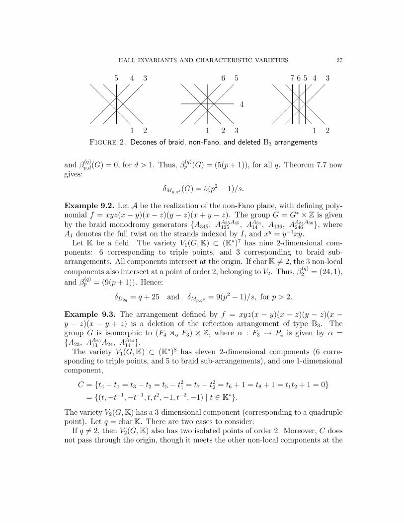
Example 9.1. Let A be the braid arrangement in C3, with defining polynomialf = xyz(x − y)(x − z)(y − z). The fundamental group is G = P4, the pure braidgroup on 4 strands.

For any field K, the variety V1(G,K) ⊂ (K∗)6 has five components, all 2-dimen-sional: four ‘local’ components, corresponding to triple points, and one ‘non-local’component, corresponding to an (essential) neighborly partition of the matroid.The components meet only at the origin, 1 = (1, . . . , 1). Moreover, V2(G,K) = 1.

Let p be a prime, and q = 0, or a prime distinct from p. From Theorem 6.5, weget:

β(q)p,0(G) = (p+ 1)(p4 + p2 − 4), β

(q)p,1(G) = 5(p+ 1),


@@

@@

@@

@@

@@

@@

1 2

345

@@

@@

@@

@@

@@

@@

1 2 3

4

56

@@

@@

@@

@@

@@

@@

1 2

34567

Figure 2. Decones of braid, non-Fano, and deleted B3 arrangements

and β(q)p,d(G) = 0, for d > 1. Thus, β

(q)p (G) = (5(p+ 1)), for all q. Theorem 7.7 now

gives:

δMp,qs (G) = 5(p2 − 1)/s.

Example 9.2. Let A be the realization of the non-Fano plane, with defining poly-nomial f = xyz(x − y)(x− z)(y − z)(x + y − z). The group G = G∗ × Z is givenby the braid monodromy generators A345, A

A35A45125 , AA34

14 , A136, AA34A36246 , where

AI denotes the full twist on the strands indexed by I, and xy = y−1xy.Let K be a field. The variety V1(G,K) ⊂ (K∗)7 has nine 2-dimensional com-

ponents: 6 corresponding to triple points, and 3 corresponding to braid sub-arrangements. All components intersect at the origin. If char K 6= 2, the 3 non-local

components also intersect at a point of order 2, belonging to V2. Thus, β(q)2 = (24, 1),

and β(q)p = (9(p+ 1)). Hence:

δD2q= q + 25 and δMp,qs = 9(p2 − 1)/s, for p > 2.

Example 9.3. The arrangement defined by f = xyz(x − y)(x − z)(y − z)(x −y − z)(x − y + z) is a deletion of the reflection arrangement of type B3. Thegroup G is isomorphic to (F4 ⋊α F3) × Z, where α : F3 → P4 is given by α =A23, A

A2313 A24, A

A2414 .

The variety V1(G,K) ⊂ (K∗)8 has eleven 2-dimensional components (6 corre-sponding to triple points, and 5 to braid sub-arrangements), and one 1-dimensionalcomponent,

C = t4 − t1 = t3 − t2 = t5 − t21 = t7 − t22 = t6 + 1 = t8 + 1 = t1t2 + 1 = 0

= (t,−t−1,−t−1, t, t2,−1, t−2,−1) | t ∈ K∗.

The variety V2(G,K) has a 3-dimensional component (corresponding to a quadruplepoint). Let q = char K. There are two cases to consider:

If q 6= 2, then V2(G,K) also has two isolated points of order 2. Moreover, C doesnot pass through the origin, though it meets the other non-local components at the


two isolated points of V2. It follows that β(q)2 = (27, 9) and β

(q)p = (11(p+ 1), p2 +

p+ 1), for p odd.If q = 2, then all the components of Vd(G,K) pass through the origin. Note that

the Galois field K = F4, obtained by adjoining to F2 the primitive 3rd root of unityω = e2π i /3, is sufficiently large with respect to Z3. The representation µ : G →Z3 = F∗

4 given by µ = (ω, ω2, ω2, ω, ω2, 1, ω, 1) belongs to C ⊂ V1(G,F4), but does

not belong to V1(G,C). Thus, by Corollary 6.3, b1(Kµ) = 8 and b(2)1 (Kµ) = 10.

Moreover, b(2)1 (Kλ) = b1(Kλ), unless λ = µ or µ. It follows that β

(2)p,d = βp,d, except

for β(2)3,1 = β3,1 + 1 = 45.

Using now Theorem 7.7, we conclude:

δD2q= 9(q + 4), δA4 = 110,

δMp,qs = ((p3 − 1)qs + p3 + 11p2 − 12)/s, otherwise.

Remark 9.4. Using the formulas from Section 8, we may compute the numberof low-index subgroups of arrangement groups. For example, if |A| = n, thena3(G) = 1

2(3n − 1) + 3δS3(G). Thus, the braid arrangement has a3 = 409, the

non-Fano plane has a3 = 1, 177, and the deleted B3 arrangement has a3 = 3, 469.The idea to use the count of index 3 subgroups as an invariant for hyper-

plane arrangement groups originates with the (unpublished) work of M. Falk andB. Sturmfels. These authors considered a pair of non-lattice-isomorphic arrange-ments of 9 planes in C3. The respective groups are in fact isomorphic (see [8,Example 7.5]). In each case, the variety V1 has twelve 2-dimensional compo-nents (8 corresponding to triple points, and 4 to braid sub-arrangements), andV2 has one 3-dimensional component (corresponding to a quadruple point). Hence:δS3 = 1

2(12(22 − 1)(3 − 1) + (23 − 1)(32 − 1)) = 64, a3 = 10, 033, and c3 = 9, 905.

10. Arrangements of transverse planes in R4

A 2-arrangement in R4 is a finite collection A = H1, . . . , Hn of transverse planesthrough the origin of R4. In coordinates (z, w) for R4 = C2, a defining polynomialfor A may be written as f = f1 · · · fn, where fi(z, w) = aiz + biz + ciw + diw. Ageneric section of A by an affine 3-plane in R4 yields a configuration of n skew linesin R3; conversely, coning such a configuration yields a 2-arrangement in R4.

The complement of the arrangement, X(A) = R4 \⋃ni=1Hi, deform-retracts onto

the complement of the link L(A) = S3 ∩⋃ni=1Hi. The link L(A) is the closure of a

pure braid β ∈ Pn. The fundamental group of the complement, G(A) = π1(X(A)),has the structure of a semidirect product of free groups: G(A) = Fn−1 ⋊ξ2 Z, whereξ is a certain pure braid in Pn−1, determined by β, see [32]. Moreover, X(A) is anEilenberg-MacLane space K(G, 1).


A 2-arrangement A is called horizontal if it admits a defining polynomial of theform f =

∏ni=1(z+aiw+biw), with ai, bi real. From the coefficients of f , one reads off

a permutation τ ∈ Sn. Conversely, given τ ∈ Sn, choose real numbers a1 < · · · < anand bτ1 < · · · < bτn . Then the polynomial f =

∏ni=1 (z − ai+bi

2w − ai−bi

2w) defines

a horizontal arrangement, A(τ), whose associated permutation is τ . The braid ξ

corresponding to A = A(τ) can be combed as ξ = ξ2 · · · ξn−1, where ξj =∏j−1

i=1 Aei,j

i,j

and ei,j = 1 if τi > τj , and ei,j = 0, otherwise.For n ≤ 5, all 2-arrangements are horizontal. For n = 6, there are 4 non-

horizontal arrangements: L, M, and their mirror images. These arrangementswere introduced by Mazurovskiı in [34]; further details about them can be found in[32]. For n = 7, there are 13 non-horizontal arrangements, see [2].

The (complex) characteristic varieties of 2-arrangement groups G = G(A) werestudied in [32]. Note that V1(G,C) is the hypersurface in (C∗)n defined by theAlexander polynomial of the link L(A); see Penne [36] for another way to computethis polynomial. We refer to [33] for more information on the resonance varietiesof 2-arrangements.

10.1. Computations of Hall invariants. We now show how to compute the

distribution β(q)p (G) of mod q Betti numbers of index p normal subgroups, and the

Hall invariants δMp,qs (G), for some 2-arrangement groups G.

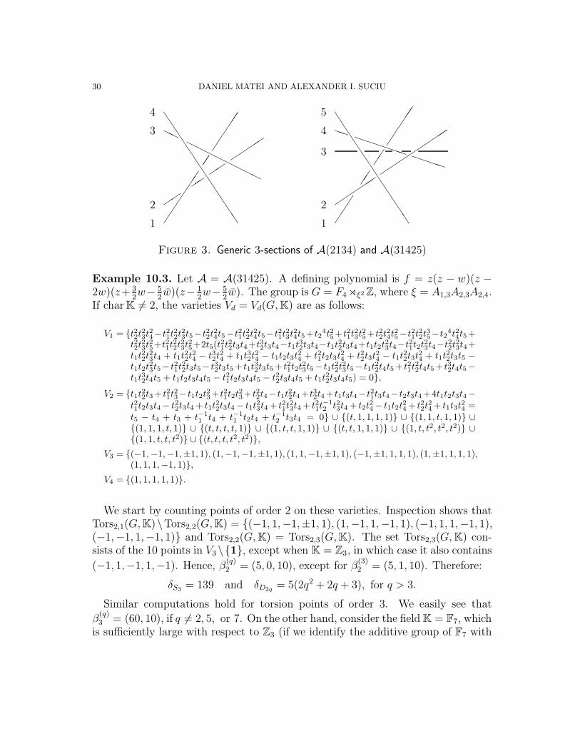
Example 10.2. Let A = A(2134) be the horizontal arrangement defined by thepolynomial f = zw(z−w)(z− 2w). The group of the complement is G = F3 ⋊ξ2 Z,where ξ = A1,2. The characteristic varieties Vd = Vd(G,K) are given by:

V1 = t4 = 1 ∪ t4 = t22,

V2 = t4 = 1, t2 = −1 ∪ t4 = t2 = t1 = 1 ∪ t4 = t2 = t3 = 1,

V3 = (1, 1, 1, 1).

Counting 2-torsion points on Vd(G,K), we see that Tors2,1(G,K)\Tors2,2(G,K) =(−1, 1,−1, 1), and Tors2,2(G,K)\Tors2,3(G,K) = (1,−1,±1, 1), (−1,−1,±1, 1),

(1, 1,−1, 1), (−1, 1, 1, 1), provided char K 6= 2. Hence, β(q)2 = (1, 6), if q 6= 2. For

an odd prime p, the count of p-torsion points yields β(q)p = (2p2 + p− 1, 2), if q ∤ 2p.

Now suppose q = 2. A sufficiently large field for the group Zp is F2s = F2(ζ),where s = ordp(2) and ζ = e2π i /p. We have V2(G,F2s) = t4 = t2 = 1, and so

Torsp,2(G,F2s) also contains the points (ζj, 1, ζ, 1), for 0 < j < p. Hence, β(2)p =

(2p2, p+ 1). By Theorem 7.7:

δD2q= 6q + 7,

δMp,2s = (p− 1)(2p2 + (p+ 1)(2s + 1))/s, for p > 2,

δMp,qs = (p− 1)(2p2 + p+ 2qs + 1)/s, for p, q > 2.


HH

HHHHHHHH

JJJJ

JJJ

JJJ

JJ1

2

3

4

PPPPPPPP PPPP

JJJ

JJ

JJJ

JJJJ1

2

3

4

5

Figure 3. Generic 3-sections of A(2134) and A(31425)

Example 10.3. Let A = A(31425). A defining polynomial is f = z(z − w)(z −2w)(z+ 3

2w− 5

2w)(z− 1

2w− 5

2w). The group is G = F4 ⋊ξ2 Z, where ξ = A1,3A2,3A2,4.

If char K 6= 2, the varieties Vd = Vd(G,K) are as follows:

V1 = t22t23t

24−t21t

22t

23t5−t22t

24t5−t21t

22t

24t5−t21t

23t

24t5+t2

4t25+t21t23t

25+t22t

24t

25−t21t

22t

35−t2

4t24t5+t22t23t25+t2

1t22t23t25+2t5(t

2

1t22t3t4+t3

2t3t4−t1t

3

2t3t4−t1t

2

2t3t4+t1t2t

2

3t4−t2

1t2t

2

3t4−t2

2t23t4+

t1t2

2t23t4 + t1t

2

2t24− t3

2t24

+ t1t3

2t24− t1t2t3t

2

4+ t2

1t2t3t

2

4+ t2

2t3t

2

4− t1t

2

2t3t

2

4+ t1t

2

2t3t5 −

t1t2t2

3t5− t2

1t22t3t5− t3

2t3t5 + t1t

3

2t3t5 + t2

1t2t

2

3t5− t1t

2

2t23t5− t1t

2

2t4t5 + t2

1t22t4t5 + t3

2t4t5−

t1t3

2t4t5 + t1t2t3t4t5 − t2

1t2t3t4t5 − t2

2t3t4t5 + t1t

2

2t3t4t5) = 0,

V2 = t1t22t3 + t21t23− t1t2t

23 + t21t2t

23 + t22t4− t1t

22t4 + t32t4 + t1t3t4− t21t3t4− t2t3t4 +4t1t2t3t4−

t21t2t3t4− t22t3t4 + t1t2

2t3t4 − t1t2

3t4 + t21t2

3t4 + t21t−1

2t23t4 + t2t

2

4 − t1t2t2

4 + t22t2

4 + t1t3t2

4 =t5 − t4 + t3 + t−1

1t4 + t−1

1t2t4 + t−1

2t3t4 = 0 ∪ (t, 1, 1, 1, 1) ∪ (1, 1, t, 1, 1) ∪

(1, 1, 1, t, 1) ∪ (t, t, t, t, 1) ∪ (1, t, t, 1, 1) ∪ (t, t, 1, 1, 1) ∪ (1, t, t2, t2, t2) ∪(1, 1, t, t, t2) ∪ (t, t, t, t2, t2),

V3 = (−1,−1,−1,±1, 1), (1,−1,−1,±1, 1), (1, 1,−1,±1, 1), (−1,±1, 1, 1, 1), (1,±1, 1, 1, 1),(1, 1, 1,−1, 1),

V4 = (1, 1, 1, 1, 1).

We start by counting points of order 2 on these varieties. Inspection shows thatTors2,1(G,K)\Tors2,2(G,K) = (−1, 1,−1,±1, 1), (1,−1, 1,−1, 1), (−1, 1, 1,−1, 1),(−1,−1, 1,−1, 1) and Tors2,2(G,K) = Tors2,3(G,K). The set Tors2,3(G,K) con-sists of the 10 points in V3\1, except when K = Z3, in which case it also contains

(−1, 1,−1, 1,−1). Hence, β(q)2 = (5, 0, 10), except for β

(3)2 = (5, 1, 10). Therefore:

δS3 = 139 and δD2q= 5(2q2 + 2q + 3), for q > 3.

Similar computations hold for torsion points of order 3. We easily see that

β(q)3 = (60, 10), if q 6= 2, 5, or 7. On the other hand, consider the field K = F7, which

is sufficiently large with respect to Z3 (if we identify the additive group of F7 with


the multiplicative subgroup of C∗ generated by ζ = e2π i /7, we may view Z3 as thesubgroup 〈ζ2〉 ⊂ F∗

7). Now Tors3,1(G,F7) \ (Tors3,2(G,F7) ∪ Tors3,1(G,C)) consistsof (ζ2, ζ4, 1, ζ4, 1), (ζ2, ζ4, ζ2, ζ4, ζ2), (ζ2, 1, ζ2, ζ4, ζ2), (ζ2, 1, ζ4, 1, ζ2), (ζ2, 1, ζ4, ζ2, 1),

together with their conjugates. Hence, β(7)3 = (65, 10). Similarly, β

(2)3 = (41, 30)

and β(5)3 = (70, 10). Therefore:

δA4 = 191, δM3,52= 330, δM3,7 = 290, and δM3,qs = 20(qs + 7)/s, for q > 7.

Remark 10.4. The resonance varieties Rd(G,C) of the arrangement A(31425) werecomputed in [33, Example 6.5]. Comparing the answer given there with the onefrom Example 10.3, we see that the variety R2(G,C) has 10 irreducible components,whereas V2(G,C) has only 9 components passing through the origin (the tenthcomponent, which does not contain 1, is not a translated torus). Thus, the tangentcone at 1 to V2(G,C) is strictly contained in R2(G,C). Another example wheresuch a strict inclusion occurs (with G the group of a certain 4-component link) wasgiven in [31, §2.3].

10.5. Classification of 2-arrangement groups. The rigid isotopy classificationof configurations of n ≤ 7 skew lines in R3 (and, thereby, of 2-arrangements ofn ≤ 7 planes in R4) was established by Viro [42], Mazurovskiı [34], and Borobiaand Mazurovskiı [2]. Clearly, if A is rigidly isotopic to A′, or to its mirror image,then G(A) ∼= G(A′). The converse was established in [32], for n ≤ 6, using cer-tain invariants derived from the characteristic varieties Vd(G,C) to distinguish thehomotopy types of the complements.

We now recover the homotopy-type classification from [32], extending it from 2-arrangements of at most 6 planes to horizontal arrangements of 7 planes, by meansof a pair of suitably chosen metabelian Hall invariants.

Theorem 10.6. For the class of 2-arrangements of n ≤ 7 planes in R4 (horizontalif n = 7), the rigid isotopy-type classification, up to mirror images, coincides withthe isomorphism-type classification of the fundamental groups. For n ≤ 6, thegroups are classified by the Hall invariant δA4; for n = 7, the Hall invariant δS3 isalso needed.

Proof. The proof is based on the computations displayed in Table 2. The firstcolumn lists the rigid isotopy classes (mirror pairs identified) of 2-arrangements A(with n = |A| ≤ 6, or n = 7 and A horizontal), according to the classification byViro, Mazurovskiı, and Borobia [42, 34, 2]. The next two columns list the Hallinvariants δS3 and δA4 for the corresponding 2-arrangement groups, G = G(A).These invariants are computed from the varieties Vd(G,F3) and Vd(G,F4), usingTheorem 7.7, as in Examples 10.2 and 10.3.


A δS3 δA4 δM3,7

A(123) 3 4 8

A(1234) 28 65 208

A(2134) 25 38 72

A(12345) 195 840 4, 560

A(21345) 168 435 1, 184

A(21435) 150 273 632

A(31425) 139 191 290

A(123456) 1, 240 10, 285 96, 800

A(213456) 1, 051 5, 182 23, 560

A(321456) 997 4, 210 12, 640

A(215436) 889 2, 752 9, 940

A(214356) 907 2, 752 7, 288

A(312546) 799 1, 780 5, 008

A(341256) 799 2, 023 5, 200

A(314256) 750 1, 474 3, 688

A(241536) 704 1, 152 2, 368

L 769 1, 631 4, 288

M 685 1, 126 1, 900

A(1234567) 7, 623 124, 124 2, 039, 128

A(2134567) 6, 408 62, 159 488, 568

A(3214567) 5, 922 47, 579 210, 024

A δS3 δA4 δM3,7

A(2143567) 5, 436 31, 541 125, 760

A(2154367) 5, 112 25, 709 83, 928

A(2165437) 5, 274 31, 541 194, 976

A(3216547) 4, 950 25, 709 145, 080

A(2143657) 4, 680 16, 961 49, 872

A(3412567) 4, 464 20, 606 74, 640

A(3125467) 4, 572 16, 961 59, 952

A(4123657) 4, 464 16, 961 72, 720

A(3126457) 4, 032 11, 129 39, 432

A(3254167) 4, 032 12, 587 41, 160

A(3142567) 4, 237 15, 227 66, 330

A(3142657) 3, 796 9, 197 25, 974

A(3145267) 3, 931 11, 651 43, 298

A(3415267) 3, 796 10, 175 34, 410

A(3154267) 3, 850 10, 751 34, 410

A(2415367) 3, 727 9, 349 26, 604

A(2415637) 3, 619 8, 709 26, 532

A(2516347) 3, 484 7, 459 20, 452

A(3625147) 3, 245 6, 349 15, 736

A(4136257) 3, 329 6, 189 15, 082

A(5264137) 3, 417 6, 819 15, 184

Table 2. Hall invariants of groups of 2-arrangements in R4.

Note that the classification can also be achieved by the Hall invariant δM3,7 (givenin the last column of Table 2), either singly (for n ≤ 6), or together with δS3 or δA4

(for n = 7 and A horizontal). Nevertheless, no combination of these 3 invariants isenough to classify the groups of non-horizontal arrangements of n = 7 planes. Itwould be interesting to know whether other Hall invariants can distinguish those13 groups.

References

[1] D. Arapura, Geometry of cohomology support loci for local systems I, J. Alg. Geom. 6

(1997), 563–597.[2] A. Borobia, V. Mazurovskiı, Nonsingular configurations of 7 lines of RP3, J. Knot Theory

Ramifications 6 (1997), 751–783.[3] G. Bredon, Sheaf theory, Second edition, Grad. Texts in Math., vol. 170, Springer-Verlag,

New York, 1997.


[4] K. S. Brown, Cohomology of groups, Corrected reprint of the 1982 original, Grad. Textsin Math., vol. 87. Springer-Verlag, New York, 1994.

[5] , The coset poset and probabilistic zeta function of a finite group, J. Algebra 225

(2000), 989–1012.[6] C. Bushnell, I. Reiner, Zeta functions of arithmetic orders and Solomon’s conjectures,

Math. Z. 173 (1980), 135–161.[7] J. Cogolludo, Topological invariants of the complements to rational arrangements, Ph.D.

thesis, Univ. of Illinois at Chicago and Univ. Complutense, Madrid, 1999.[8] D. Cohen, A. Suciu, The braid monodromy of plane algebraic curves and hyperplane ar-

rangements, Comment. Math. Helvetici 72 (1997), 285–315.[9] , Characteristic varieties of arrangements, Math. Proc. Cambridge Phil. Soc. 127

(1999), 33–53.[10] C. Curtis, I. Reiner, Methods of representation theory. Vol. 1 (reprint of the 1981 edition),

John Wiley & Sons, New York, 1990.[11] D. Eisenbud, Commutative algebra with a view towards algebraic geometry, Grad. Texts

in Math., vol. 150, Springer-Verlag, New York, 1995.[12] M. Falk, Arrangements and cohomology, Ann. Combin. 1 (1997), 135–157.[13] R. H. Fox, Free differential calculus. III. Subgroups, Ann. of Math. 64 (1956), 407–419.[14] , Metacyclic invariants of knots and links, Canad. J. Math. 22 (1970), 193–201.[15] The GAP Group, GAP–Groups, Algorithms, and Programming, Version 4.1, Aachen,

St. Andrews, 1999; available at http://www-gap.dcs.st-and.ac.uk/~gap.[16] D. Grayson, M. Stillman, Macaulay 2: a software system for algebraic geometry and com-

mutative algebra; available at http://www.math.uiuc.edu/Macaulay2.[17] M. Hall, Subgroups of finite index in free groups, Canad. J. Math 1 (1949), 187–190.[18] P. Hall, The Eulerian functions of a group, Quart. J. Math 7 (1936), 134–151.[19] J. Hempel, Homology of coverings, Pacific J. Math. 112 (1984), 83–113.[20] , Homology of branched coverings of 3-manifolds, Canad. J. Math. 44 (1992), 119–

134.[21] E. Hironaka, Alexander stratifications of character varieties, Annales de l’Institut Fourier

(Grenoble) 47 (1997), 555–583.[22] J. H. Kwak, J.-H Chun, J. Lee, Enumeration of regular graph coverings having finite

abelian covering transformation groups, SIAM J. Discrete Math. 11 (1998), 273–285.[23] A. Libgober, On the homology of finite abelian coverings, Topology. Appl. 43 (1992),

157–166.[24] , Characteristic varieties of algebraic curves, arXiv:math.AG/9801070.[25] , First order deformations for rank one local systems with non vanishing cohomol-

ogy, Topology Appl. (to appear).[26] A. Libgober, S. Yuzvinsky, Cohomology of the Orlik-Solomon algebras and local systems,

Compositio Math. 21 (2000), 337–361.[27] D. Lind, A zeta function for Zd-actions, In: Ergodic theory of Zd actions (Warwick, 1993–

1994), London Math. Soc. Lecture Note Ser., vol. 228, Cambridge Univ. Press, Cambridge,1996, pp. 433–450.

[28] C. Livingston, Lifting representations of knot groups, J. Knot Theory Ramifications 4

(1995), 225–234.[29] A. Lubotzky, Counting finite index subgroups, In: Groups ’93, Galway/St. Andrews, Vol. 2,

London Math. Soc. Lecture Note Ser., vol. 212, Cambridge Univ. Press, Cambridge, 1995,pp. 368–404.

http://www-gap.dcs.st-and.ac.uk/~gap

http://www.math.uiuc.edu/Macaulay2

http://front.math.ucdavis.edu/math.AG/9801070


[30] I. G. Macdonald, Symmetric functions and Hall polynomials, Second edition. With con-tributions by A. Zelevinsky, Oxford Math. Monographs, Oxford Univ. Press, New York,1995.

[31] D. Matei, Fundamental groups of links and arrangements: characteristic varieties, res-

onance varieties, and finite index subgroups, Ph.D. thesis, Northeastern Univ., Boston,MA, 1999.

[32] D. Matei, A. Suciu, Homotopy types of complements of 2-arrangements in R4, Topology39 (2000), 61–88.

[33] , Cohomology rings and nilpotent quotients of real and complex arrangements, In:Arrangements–Tokyo 1998 (M. Falk, H. Terao, eds.), Adv. Stud. Pure Math., vol. 27,Math. Soc. Japan, Kinokuniya, Tokyo, 2000, pp. 185–215.

[34] V. Mazurovskiı, Configurations of six skew lines (Russian), Zap. Nauchn. Sem. LeningradOtdel. Mat. Inst. Steklov (LOMI) 167 (1988), 121–134; translation in J. Soviet Math. 52

(1990), 2825–2832.[35] A. D. Mednykh, Unramified coverings of compact Riemann surfaces (Russian), Dokl. Akad.

Nauk SSSR 244 (1979), 529–532; English translation: Soviet Math. Dokl. 20 (1979), 85–88.

[36] R. Penne, The Alexander polynomial of a configuration of skew lines in 3-space, Pacific J.Math. 186 (1998), 315–348.

[37] D. Robinson, A course in the theory of groups, Grad. Texts in Math., vol. 80, Springer-Verlag, New York, 1996.

[38] S. Roman, Field theory, Grad. Texts in Math., vol. 158, Springer-Verlag, New York, 1995.[39] M. Sakuma, Homology of abelian coverings of links and spatial graphs, Canad. J. Math.

47 (1995), 201–224.[40] R. Stanley, Enumerative combinatorics. Vol. 2, Cambridge Studies in Advanced Math.,

vol. 62, Cambridge Univ. Press, Cambridge, 1999.[41] A. Suciu, Translated tori in the characteristic varieties of complex hyperplane arrange-

ments, Topology. Appl. (to appear), arXiv:math.AG/9912227.[42] O. Viro, Topological problems concerning lines and points of three-dimensional space, Dokl.

Akad. Nauk. SSSR 284 (1985), 1049–1052; English transl., Soviet Math. Dokl. 32 (1985),528–531.

[43] L. Weisner, Some properties of prime-power groups, Trans. Amer. Math. Soc. 38 (1935),485–492.

Department of Mathematics, University of Rochester, Rochester, NY 14627

E-mail address : [email protected]

Department of Mathematics, Northeastern University, Boston, MA 02115

E-mail address : [email protected]: http://www.math.neu.edu/~suciu

http://front.math.ucdavis.edu/math.AG/9912227

mailto:[email protected]

mailto:[email protected]

http://www.math.neu.edu/~suciu/

Hall invariants, homology of subgroups, and characteristic varieties

Documents

Transcript of Hall invariants, homology of subgroups, and characteristic varieties