Honors Year Project Report

Fascinating Invariants

By

Toh Xiu Ping

Department of Computer Science

School of Computing

National University of Singapore (NUS)

2007/2008

Project Number: H114130

Project Advisors: Prof Wong Limsoon

Deliverables:

Report: 1 Volume

2

Honors Year Project Report

Fascinating Invariants

By

Toh Xiu Ping

Department of Computer Science

School of Computing

National University of Singapore (NUS)

2007/2008

3

Abstract

It’s the computing world… Explored, explained and examined.

Explored. We will explore the role of invariant and its exploitation in problem solving.

Problems studied in this paper include those which we might have encountered before in

our daily lives, in elementary computing, in database design as well as in artificial

intelligence.

Explained. The solution or solutions will be explained plainly to bring out the simplicity

and elegance of invariant. In the course, we will learn to appreciate the use and

exploitation of invariants in these solutions.

Examined. We will examine how the concept of invariant can be applied in the area of

research topics even beyond the area of computing, particularly in the field of biology.

4

Acknowledgements

First and foremost, I would like to thank my supervisor, Prof Wong Limsoon. Without

his invaluable advice, kind patience and guidance, this project would not be possible.

My heartfelt gratitude also goes out to everyone who had offered their assistance for the

duration of the whole project for their advice, feedback and support.

Last but not least, I would like to show my gratitude to the evaluators of this project for

taking time off their busy schedules to access this project.

5

List of Figures and Tables Figures

FIGURE 1 TRACING OF THE LOCATION OF THE CARD IN THE 21 CARD TRICK................................ 13

FIGURE 2 DEFINITION OF EXPONENTIAL AND POWER FUNCTIONS. ............................................... 16

FIGURE 3 AN EXAMPLE OF A PUZZLE – TOWER OF HANOI WITH 3 PEGS ....................................... 18

FIGURE 4 SOLUTION OF 4 QUEEN PUZZLE IS A SUBSET OF 5 QUEEN PUZZLE. ................................ 20

FIGURE 5 STEP BY STEP SOLUTION TO A 4 QUEEN PUZZLE. ........................................................... 21

FIGURE 6 ILLUSTRATING THE 4 MAIN BOUNDARIES IN THE DUTCH NATIONAL FLAG. ................. 23

FIGURE 7 EXAMPLE OF DUTCH NATIONAL FLAG PUZZLE. ........................................................... 25

FIGURE 8 UPDATE ANOMALIES. .................................................................................................... 26

FIGURE 9 INSERTION ANOMALIES. ................................................................................................ 26

FIGURE 10 DELETION ANOMALIES. ............................................................................................... 27

FIGURE 11 EXAMPLE OF CONVERTING A BAD DESIGN TO A GOOD DATABASE DESIGN (BCNF). .. 29

FIGURE 12 GENETIC INFORMATION OF TAIWANESE, SOLOMON ISLANDERS AND RAROTONGANS.

.............................................................................................................................................. 32

FIGURE 13 HYPOTHETICAL TRACE OF THE MIGRATION OF THE POLYNESIANS. IMAGE CREDIT: [8]

.............................................................................................................................................. 33

FIGURE 14 THE METHOD – GUILT BY ASSOCIATION IN PREDICTING FUNCTION OF AN UNKNOWN

PROTEIN. ............................................................................................................................... 35

FIGURE 15 ILLUSTRATE THE CONCEPT OF EMERGING PATTERN FROM INVARIANTS. .................... 36

6

Table of Contents

ABSTRACT .................................................................................................................................................. 3 ACKNOWLEDGEMENTS ......................................................................................................................... 4 LIST OF FIGURES AND TABLES ........................................................................................................... 5 CHAPTER 1 – INTRODUCTION.............................................................................................................. 8

1.1 BACKGROUND ...................................................................................................................................... 8 1.2 OBJECTIVES AND SCOPE ....................................................................................................................... 8 1.3 ORGANIZATION OF REPORT .................................................................................................................. 8

CHAPTER 2 – INVARIANT IN OUR DAILY LIFE ............................................................................. 10 2.1 THE IQ QUESTION – WHO IS LARRY? ................................................................................................. 10

2.1.1 The Answer ................................................................................................................................ 10 2.1.2 The Proof ................................................................................................................................... 10 2.1.3 The Invariant.............................................................................................................................. 11

2.2 THE 21 CARD TRICK........................................................................................................................... 11 2.2.1 The Trick .................................................................................................................................... 11 2.2.2 The Secret Revealed – Invariant ................................................................................................ 12 2.2.3 The Proof ................................................................................................................................... 13

2.3 CRIME SCENE INVESTIGATION............................................................................................................ 14 2.3.1 The Invariant.............................................................................................................................. 14 2.3.2 The Discovery ............................................................................................................................ 15

CHAPTER 3 – INVARIANTS IN RECURSION .................................................................................... 16 3.1 CALCULATING POWER/EXPONENTIAL FUNCTIONS ............................................................................. 16

3.1.2 Exploitation of Invariant....................................................................................................... 16 3.2 TOWER OF HANOI ............................................................................................................................... 17

3.2.1 The Invariant ........................................................................................................................ 18 3.2.2 The Solution.......................................................................................................................... 18

3.3 N-QUEENS PUZZLE ............................................................................................................................. 19 3.3.1 The Invariant ........................................................................................................................ 19 3.3.2 The Solution.......................................................................................................................... 20

CHAPTER 4 – MAINTAINING INVARIANTS..................................................................................... 22 4.1 THE DUTCH NATIONAL FLAGS ........................................................................................................... 22

4.1.1 The Invariant ........................................................................................................................ 22 4.1.2 The Solution.......................................................................................................................... 22 4.1.3 An Example........................................................................................................................... 24

4.2 A GOOD DATABASE DESIGN............................................................................................................... 25 4.2.1 Update/Insert/Delete Anomalies........................................................................................... 26 4.2.2 Invariant in a Good Database Design.................................................................................. 27 4.2.3 An Example........................................................................................................................... 28

CHAPTER 5 – APPLICATION OF INVARIANTS IN BIOLOGY...................................................... 30 5.1 INVARIANTS IN EVOLUTION................................................................................................................ 30

5.1.1 Genetic Recombination – Mitochondria Control Region is Conserved................................ 30 5.1.2 Mutation – Mutations are cumulative................................................................................... 31 5.1.3 The Origin of Polynesians .................................................................................................... 31

5.2 PREDICTING PROTEIN FUNCTION ........................................................................................................ 33 5.2.1 What are Proteins?............................................................................................................... 33 5.2.2 The Invariant ........................................................................................................................ 34 5.2.3 Emerging Patterns from Invariant........................................................................................ 35

7

CHAPTER 6 – CONCLUSION................................................................................................................. 37 APPENDIX A – PSEUDO CODE OF SOLVING POWER FUNCTION I .......................................... 40 APPENDIX B – PSEUDO CODE OF SOLVING POWER FUNCTION II ......................................... 40 APPENDIX C – PSEUDO CODE FOR TOWER OF HANOI .............................................................. 41

8

Chapter 1 – Introduction

1.1 Background

Due to the huge dependence on technology today, there are many research topics

undergoing at every moment. But underlying most of these research problems, they share

a common concept. This concept is what we will investigate in this paper. It is called the

invariant.

Many problems in research and even in our daily lives have an underlying invariant. An

invariant is something, usually a condition that does not change regardless of any external

changes or manipulation of the data. They are usually the pre-defined objective of the

problem. Often time, if we are able to identify the key invariant of each problem, we will

be able to find the key to the solution.

1.2 Objectives and Scope

The objective of this project is to exhibit the concept of invariant and how they can be

exploited to solve different types of problems. In this report, we will look at problems

ranging from our everyday life, elementary computing problems and also various

specializations of computing areas such as database design, artificial intelligence.

Lastly, we will explore the role of invariant beyond the walls of computing, particularly

in the field of biology. These problems are solved by identifying and exploiting the

various forms of invariants to discover the solutions in a classy manner.

1.3 Organization of Report

We will look at the various problems under four main categories.

9

Section 2 will explore invariants in our daily life. We will start off with an IQ question

(Who is Larry?) followed by a familiar magic trick (The 21 card trick) then finally, we

will take a look into how invariant has played a role in crime scene investigation (The

blood that can tell time). In these three examples, we will highlight how identifying the

key invariant will eventually lead us to the solution. This section aims to help reader

grasp the concept of invariant in simple terms.

Section 3 will showcase three problems where invariant is exploited to reduce the

problem size and solve them in the most elegant manner. They are Calculating

Exponential/Power Functions, Tower of Hanoi and lastly, the N-queen Puzzle.

Section 4 investigates problems where the solution will come into view simply by

enforcing the invariant identified. Checking and correcting violations of invariant is the

key method of solving these problems under this section, namely The Dutch National

Flag and A Good Database Design.

In the first problem under both section 3 and 4, we will also witness how different

invariants of different forms can lead us to a more efficient solution.

Section 5 will take us through the application of invariant in the field of biology. Such

invariants give us a clue to the secrets behind our ancestries. This will be depicted in the

problem of tracing the Origin of Polynesians. Secondly, we will see how invariants help

us in Predicting Protein Function.

10

Chapter 2 – Invariant in Our Daily Life In this section, we will explore invariants in our daily life. Through these familiar

problems, I hope that readers will be able to grasp the concept of invariant in simple

terms. We will first start off with an IQ question (Who is Larry?) followed by an

interesting magic trick (The 21 cards trick) then finally, we will take a look into how

invariant has played a role in crime scene investigation (The blood that can tell time).

2.1 The IQ Question – Who is Larry?

If some of you can remember, there was this popular IQ question being asked when we

were in high school.

The question goes like this: “A pair of twin – Larry and Harry is presented to you. The

twin are identical except that Harry will always tell the truth and Larry will always lie.

You are allowed to ask any question to any one of them to find out who is Larry. How are

you going to go about doing it?”

2.1.1 The Answer

The solution is very simply by asking either of the boys: “What do you think the other

boy, Boy B, will tell me if I were to ask him if Boy B is Larry?” The solution is that

simple and straight forward. You will only need to ask one question to either one of them.

Regardless of who you ask, you will be able to solve the question!

2.1.2 The Proof

If we happen to ask Larry the question, he would invert the truth and say that the other

boy, who is Harry, will deny that he is NOT Larry. If we happen to ask Harry the same

question, he will tell us that Larry who is a liar will deny that he IS Larry. In both

scenarios, we will obtain an inverted answer which does not change regardless of who we

11

ask. This is what we defined as the invariant in Section 1.1. Knowing that whoever we

ask will give us the incorrect answer, we can find out who is Larry by doing the opposite.

2.1.3 The Invariant

Let us explore how we come to this discovery. The fact that remains unchanged

throughout the whole incident is that one of the boys will lie while the other will tell the

truth. If we represent their answer in terms of 1 and 0, meaning 1 for the true and 0 for

the false answer, we will realize that we will not be able to make use of this invariant

directly. In other words, this invariant is not useful to us in its current form. However, if

we look at the relationship between the two, we will discover an underlying invariant

which will miraculously bring us to our solution. That is 1 X 0 = 0 and 0 X 1 = 0. We

will always obtain the false answer if we ask any of the boys what the other boy would

say. After we identified this invariant, we will be able to obtain the answer by simply

inverting the answer given to us. The case that Boy A who says that Boy B will deny his

identity of Larry implies that Boy B is Larry and hence, Boy A will have to be Harry!

2.2 The 21 Card Trick

Many card tricks that are performed by magicians will go something like this: random

manipulations of a deck of cards then being able to deal your card out from the random

deck at the end. How are they able to do that? Is it really magic? Here, we will explore a

common magic trick which has been unveiled.

2.2.1 The Trick

The trick, as the name gave it away, involves random manipulation of 21 cards and

finally dealing out the card which you have chosen at the beginning of the trick. This is

how the trick goes:

12

The magician will ask you to remember any one of the cards from a deck of 21

cards in your mind as your card. You do not have to tell him where or what the

card is.

He will then deal the 21 cards face down, from top to bottom and left to right, into

3 equal piles.

Next, he will fan individual piles to you and ask you to look for the pile of cards

which contains your card and pass the pile back to him.

Again, he will stack up the 3 piles on top of each other and redistribute, from top

to bottom and left to right, into 3 equal piles.

He will repeat step (iii) and (iv) 2 more times.

Finally, he will be able to deal your card right out from the rest of the 21 cards.

2.2.2 The Secret Revealed – Invariant

The invariant of this trick is the repetitive procedure of stacking and redistributing the

cards into 3 equal piles. The secret behind this is that each time the magician stack up the

cards, the pile that contains the card which you have chosen at the beginning of the trick

is being placed in the middle of the other 2 piles. By doing so, the magician is actually

putting constraints to where your card can move to. In this paper, we refer to these

constraints as invariant – something which will remain the same or constant regardless of

what changes was made.

At the first distribution, we would have reduced the location of the card by a third since

we are placing the pile of 7 cards, containing the chosen card, in the middle of the 21

cards deck. At the second distribution, the chosen card will have to be in one of the

locations below:

the fourth or fifth card of the first pile;

the third, fourth or fifth card of the middle pile; or

the third or fourth card of the last pile.

If the chosen card was in the third position in its pile, it would be in the 4th position in its

new pile in the next distribution. If the chosen card was in the 4th position in its pile, it

13

would be in the 4th position of the middle pile in the next distribution. If the chosen card

was in the 5th position in its pile, it would be in the 4th position of its new pile in the next

distribution. Hence, at the 3rd distribution, the chosen card will land as the middle card

(i.e., 4th card in the middle pile). This is the key invariant of the trick!

The trick will only work if the invariant is hidden from the audience, and only the

magician knows it in his heart. By keeping the invariant in mind, the magician can then

put up a good show. And only an observant audience will be able to identify the key

invariant to understand the magic. Similar to the rest of the problems explored in this

paper, we will look at how invariant of various forms help us to solve the problem in the

most elegant manner.

2.2.3 The Proof

Let us number the cards as the following:

pile 1: 11, 12, 13, 14, 15, 16, 17;

pile 2: 21, 22, 23, 24, 25, 26, 27;

pile 3: 31, 32, 33, 34, 35, 36, 37.

Without loss of generality, let us assume the chosen card is in pile 1. After the first

distribution, we have the following:

Figure 1 Tracing of the location of the card in the 21 card trick.

The positions with 11, 12, 13, 14, 15, 16, 17 indicates where the cards in the chosen pile

will have to go in the next distribution respectively. Specifically, the 3rd card (which

could be either 11 or 12) must go to 4th position of the first pile (marked by 13), the 5th

card (which could be either 16 or 17) must go to the 4th position of the third pile (marked

14

by 15), and the 4th card (which could be 13, 14, or 15) must go to the 4th position of the

middle pile (marked by 14). The allowable moves are indicated by arrows. We can see

that after two moves, the chosen card must land in the 4th position of the middle pile!

This constraint in movement of the card is similar if the chosen card is in the 2nd or 3rd

pile.

2.3 Crime Scene Investigation

In crime scene investigation, blood evidence provides vital information to the police. A

spatter pattern of the blood can indicate the way the victim was attacked and further DNA

test can tell whose blood it belonged to. However, there was no way of knowing how old

a blood sample is.

This ambiguity was brought to Clifton Bishop’s attention, a molecular geneticist at West

Virginia University when he read about the O.J. Simpson murder case. There was blood

sample from Simpson’s former wife, Nicole, found in O.J.’s car which the prosecutor

claimed that was a product of murder. However, the defense argued that the blood had

come from a cut a few months earlier.

Clifton Bishop could not believe that DNA analysis is unable to differentiate a months’

old blood from a few days old blood. Hence, he was determined to create a technique that

he hopes will change that. His idea is modeled on the carbon-14 system used to estimate

the age of fossils.

2.3.1 The Invariant

Since we are looking at the age of a blood sample, we should focus on finding an

invariant with respect to time. Thus, a question to ask will be: Are there any genetic

materials in blood that will remain the same with respect to time? In this respect, Bishop

15

has identified that the rate of degradation of RNA strands with respect to strand length

remains the same.

2.3.2 The Discovery

After analyzing the rate of degradation, he made the observation that longer strands of

RNA tend to degrade at a higher rate than shorter ones. Hence, Bishop theorized that the

age of a given blood sample could be estimated by calculating the ratio of long strands to

short ones.

However, there are still some shortcomings which should be improved on before this

technology is considered launched. Firstly, there is a caveat that the amount of RNA of

different lengths is different for different person at different time. Secondly, blood is

extremely sensitive to the environment. The latter would not be an issue where

environment is relatively stable, for instance inside a house. This technology will most

probably undergo further development over the years before we can see its official launch

in the commercial world.

16

Chapter 3 – Invariants in Recursion In this section, we will look at three problems which are solved by similar method -

identifying the invariant that remain consistent in the solutions of the same problem

regardless of the problem size. Having identified the invariant, we can then reduce the

given problem to smaller sets which are trivial.

3.1 Calculating Power/Exponential Functions

A power function is defined as i^j = i x i x … x i (j times) as depicted in Figure 2.

Figure 2 Definition of exponential and power functions.

Calculating exponential or power functions has been made very easy with the use of

calculators. Answers can be obtained in split seconds. In this section, we will peek into

the world of calculators.

3.1.2 Exploitation of Invariant

Underlying every problem, there will always be an invariant. In this case, we can write

i^j = i * i^(j-1). This is the invariant which will lead us to the answer. The solution

requires recursively multiplying the accumulated value with i as we reduce the value of j

by 1. The solution is simple and obvious because we can clearly see it from the invariant

identified. The pseudo code of the solution can be found in Appendix A.

However, in the following paragraph, we will be able to see how invariant of another

form in the same problem will lead us to a more efficient solution. The invariant is the

fact that i^(2j) = (i^j) * (i^j). With this invariant, though very similar to the previous

one, we are able to increase the efficiency of the program! Notice that the problem is now

17

reduced into two equal sets which are exactly the same. Hence, only one of them needs to

be computed and reused for the other. In this way, we are saving half the computation

cost at each recursion call! In the case where the parity of j is odd, j will be reduced by 1

(making it even) and multiply the accumulated value with i once before we recursively

call the function again with the value of j now being even. The solution of this second

invariant can be found in Appendix B.

3.2 Tower of Hanoi

There was a legend saying that a few centuries ago, a stack of 64 gold disks was given to

the priests in a Hindu temple. The disks were stacked with the largest disks at the bottom

while the smallest at the top in one of the three poles given to them. The task that was

given to them was to transfer all the disks from one pole to another. However, while

doing that, a larger disk could never be placed on top of a smaller one and they can only

move one disk at a time. When they finished their work, the legend said, the temple

would crumble into dust and the world would vanish. [3]

This legend has inspired a French mathematician, Edouard Lucas to invent this puzzle

called the Tower of Hanoi. The rule of the puzzle is similar to the legend, as follows:

There are three pegs (A, B and C where A is the initial peg where all the disks are stacked

on and C being the destination of the disks).

The puzzle starts with a tower of n disks on peg A neatly stacked in order of size, the

smallest at the top, thus making a conical shape.

The objective of the game is to move all the disks from peg A to peg C obeying the

following rules:

i. Only one disk may be moved at a time.

ii. No bigger disk may be placed on top of a smaller disk.

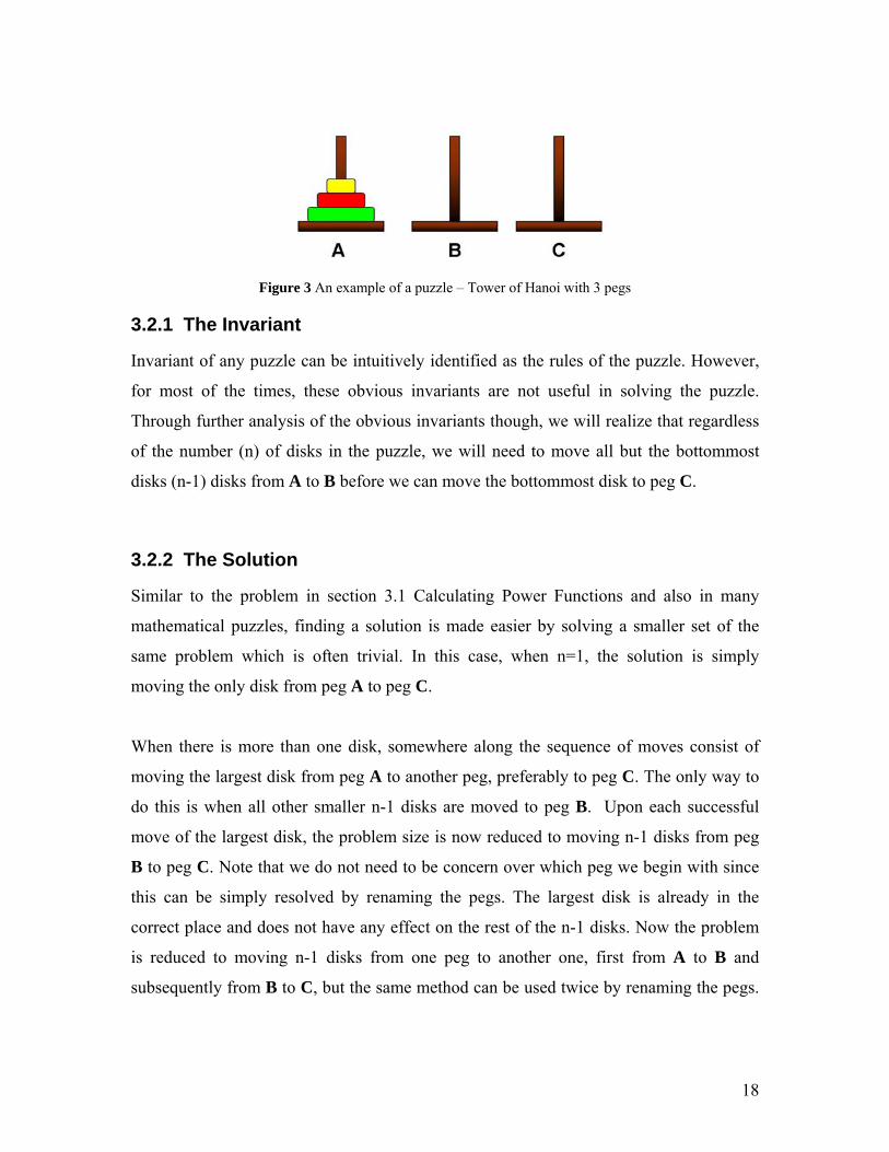
Figure 3 shows an example of a puzzle with 3 disks.

18

Figure 3 An example of a puzzle – Tower of Hanoi with 3 pegs

3.2.1 The Invariant

Invariant of any puzzle can be intuitively identified as the rules of the puzzle. However,

for most of the times, these obvious invariants are not useful in solving the puzzle.

Through further analysis of the obvious invariants though, we will realize that regardless

of the number (n) of disks in the puzzle, we will need to move all but the bottommost

disks (n-1) disks from A to B before we can move the bottommost disk to peg C.

3.2.2 The Solution

Similar to the problem in section 3.1 Calculating Power Functions and also in many

mathematical puzzles, finding a solution is made easier by solving a smaller set of the

same problem which is often trivial. In this case, when n=1, the solution is simply

moving the only disk from peg A to peg C.

When there is more than one disk, somewhere along the sequence of moves consist of

moving the largest disk from peg A to another peg, preferably to peg C. The only way to

do this is when all other smaller n-1 disks are moved to peg B. Upon each successful

move of the largest disk, the problem size is now reduced to moving n-1 disks from peg

B to peg C. Note that we do not need to be concern over which peg we begin with since

this can be simply resolved by renaming the pegs. The largest disk is already in the

correct place and does not have any effect on the rest of the n-1 disks. Now the problem

is reduced to moving n-1 disks from one peg to another one, first from A to B and

subsequently from B to C, but the same method can be used twice by renaming the pegs.

19

The same strategy can be used to reduce the n-1 problem to n-2, n-3, and so on until only

one disk is left.

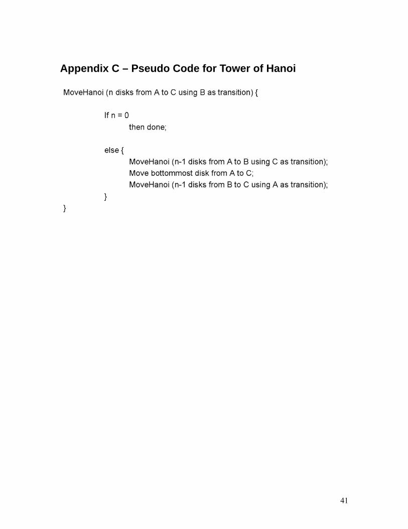
This algorithm can be schematized as follows. The following is a procedure for moving a

tower of n disks from a peg A onto a peg C, with B being the transition peg:

Step 1: If n>1 then first use this procedure to move the n-1 smaller disks from peg

A to peg B.

Step 2: Now the largest disk, i.e. disk n-1 can be moved from peg A to peg C.

Step 3: If n>1 then again use this procedure to move the n-1 smaller disks from

peg B to peg C.

The pseudo code of this puzzle can be found in Appendix C.

3.3 N-Queen Puzzle

The N-queens puzzle is one of the most famous puzzles we will encounter in most

artificial intelligence courses. The puzzle is the challenge of placing n chess queens on a

n×n chessboard (where n ≥ 4) such that no two queens will attack each other. It would be

obvious that for a 1 X 1 board, the solution is trivial and there will be no solutions for 2 X

2 and 3 X 3 boards.

Similar to any chess game, a queen can attack vertically, horizontally and diagonally. In

other words, a solution requires that no two queens share the same row, column, or

diagonal.

3.3.1 The Invariant

The rule of the puzzle is the invariant that imposes constraints to where we can place a

queen. We can solve the puzzle by generating all possible permutations of the queen

placement. Then for each possible solution, we would check if there is any violation of

20

the invariant. However this method is not favorable and very inefficient since there are

too many redundant and obviously wrong solutions being generated.

Through further analysis to the obvious invariant, we realize that regardless of the value

of n, the solution to a (n-1) queen puzzle is a subset of a n-queen puzzle. Figure 4 shows

an example where the solution to a 4 queen puzzle is a subset of a 5 queen puzzle.

Figure 4 Solution of 4 queen puzzle is a subset of 5 queen puzzle.

3.3.2 The Solution

Instead of reducing the n from n to 4 like how we did for the problem in Section 3.1 –

Tower of Hanoi, we build the solution from n=4 to the desired n. Figure 5 illustrate the

solution to a 4 queen puzzle step by step.

• Add one queen on one row at every step

• If a queen that creates conflict is placed, discard the partial solution

• Undo the step causing the conflict

• Place the queen on another possible position (backtracking)

• Continue adding more queens until n queens are placed

21

Figure 5 Step by step solution to a 4 queen puzzle.

22

Chapter 4 – Maintaining Invariants This section will investigate two main problems where the solution will come into view

by itself simply by enforcing the invariant identified. Enforcing invariant in this section

refers to checking and correcting violations of invariant throughout the entire data given.

This method of solving these problems has simplified complicated problems. The

problems covered in this section are The Dutch National Flag and A Good Database

Design.

4.1 The Dutch National Flag

The Dutch national flag consist of three main colors. They are namely red, white and

blue. Given any number of balls of these three colors arranged randomly in a line, the

task is to arrange them such that all balls of the same color are together and in the order

of red, white and blue. [6] This problem can be viewed in terms of rearranging or sorting

elements in an array.

4.1.1 The Invariant

In almost every puzzle, the invariant is the rule of the puzzle. It is not any different in this

case. The ultimate aim of this puzzle is to arrange the elements of the array in a particular

order. For instance, we can pre-define the order to be red, followed by white then

followed by blue. This puzzle is considered solved once all the same colored elements of

the array are together and in this pre-defined order. In other words, the puzzle is solved

once the invariant is being maintained throughout the entire array.

4.1.2 The Solution

We can go about maintaining the invariant by picking out random pairs of elements,

check their order and swap them if they violate the invariant (i.e., if they are in the wrong

order). If the two elements picked are the same color or in the correct order, we do not

23

have to swap them. This checking process will be repeated so that the invariant is

maintained throughout the entire array. When this is achieved, all elements in the array

will be in the correct order.

The total number of violations at any one time is the number of element pairs which are

in the wrong order. Each swap action will reduce the number of violations by one.

Similar to the problem in Section 3.1 in Calculating Exponential/Power, this reduction by

one after each swap is inefficient. We need to scan through the array with n elements (n x

n) times to ensure every element of the array is in the correct order. In computing, we

refer this as run time and represent it with the big O notation i.e., O (n2).

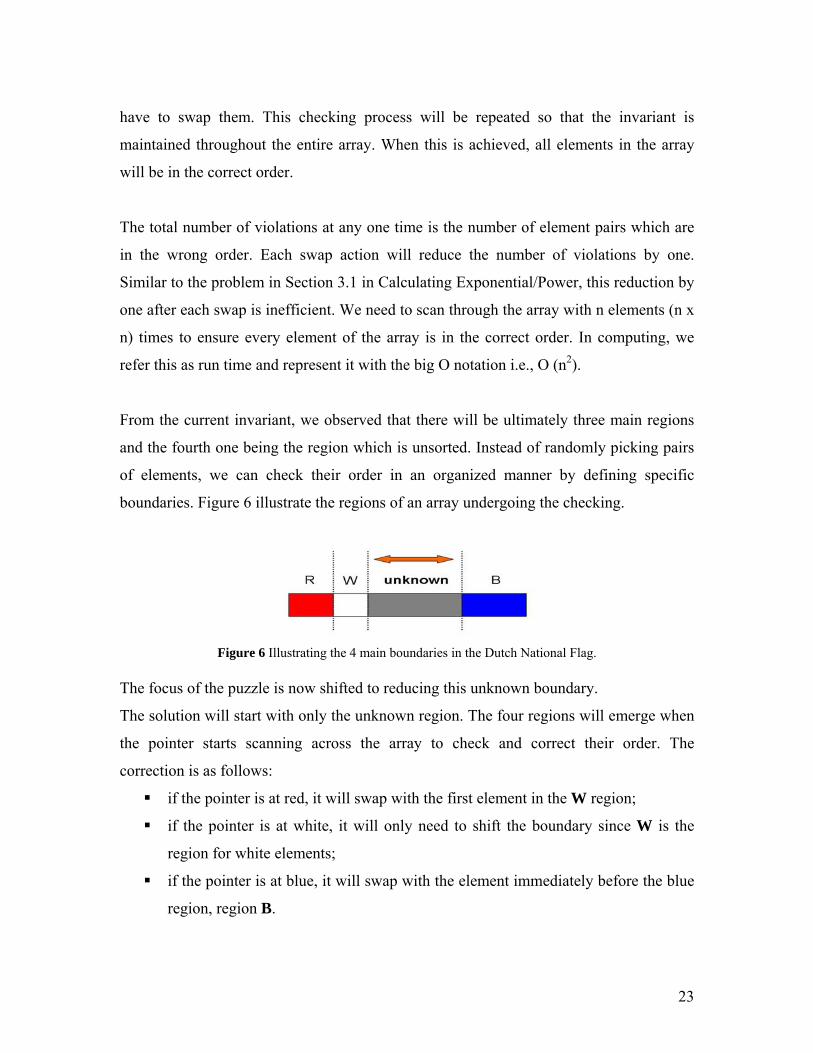
From the current invariant, we observed that there will be ultimately three main regions

and the fourth one being the region which is unsorted. Instead of randomly picking pairs

of elements, we can check their order in an organized manner by defining specific

boundaries. Figure 6 illustrate the regions of an array undergoing the checking.

Figure 6 Illustrating the 4 main boundaries in the Dutch National Flag.

The focus of the puzzle is now shifted to reducing this unknown boundary.

The solution will start with only the unknown region. The four regions will emerge when

the pointer starts scanning across the array to check and correct their order. The

correction is as follows:

if the pointer is at red, it will swap with the first element in the W region;

if the pointer is at white, it will only need to shift the boundary since W is the

region for white elements;

if the pointer is at blue, it will swap with the element immediately before the blue

region, region B.

24

After each check, it will shift the boundary and move to the next element. It will only

stop once the unknown boundary coincides with the boundary of B region. When this

happens, it also indicates that the unknown region has diminished and all elements has

been checked and are in the correct region. This solution is not only correct but also gives

us a better run time of O (n). This is because we only need to scan the array once.

4.1.3 An Example

Figure 7 shows a step by step example on how the swapping and shifting of the

boundaries work. When we are first given the array, we do not know the order.

Therefore, the entire array is regarded as the unknown region which we are supposed to

sort after scanning through once. We can observe that the order of the elements is being

corrected as the three main regions slowly developed. At the same time, the size of the

unknown region is reduced by one after each step.

25

Figure 7 Example of Dutch National Flag Puzzle.

4.2 A Good Database Design

A database is a collection of data or records stored in the computer, usually in a table

form. The amount of data can be very small or it can be very huge. When dealing with

huge amount of data, a good database structure is essential. This is because huge database

is susceptible to update, insert and delete anomalies. These anomalies will create

confusion and errors when queries are sent to the computer. [7]

26

4.2.1 Update/Insert/Delete Anomalies

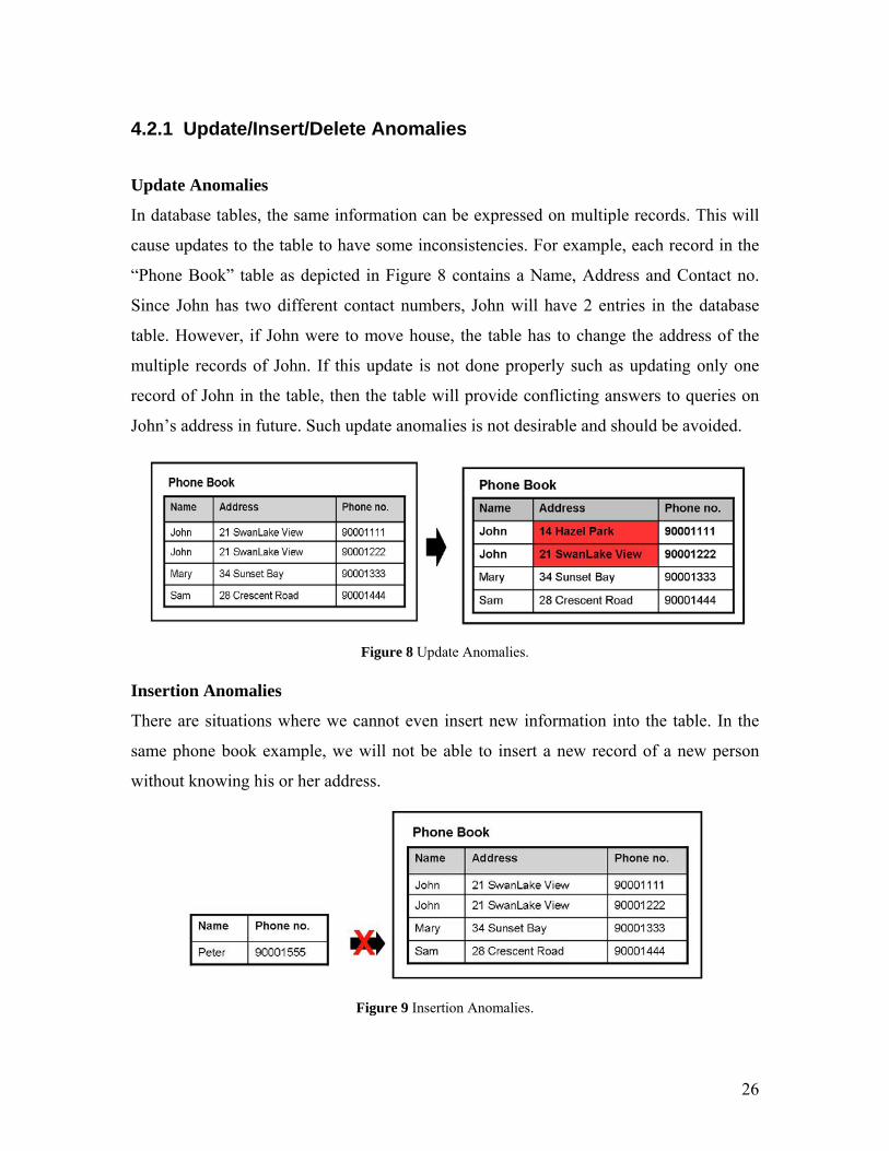
Update Anomalies

In database tables, the same information can be expressed on multiple records. This will

cause updates to the table to have some inconsistencies. For example, each record in the

“Phone Book” table as depicted in Figure 8 contains a Name, Address and Contact no.

Since John has two different contact numbers, John will have 2 entries in the database

table. However, if John were to move house, the table has to change the address of the

multiple records of John. If this update is not done properly such as updating only one

record of John in the table, then the table will provide conflicting answers to queries on

John’s address in future. Such update anomalies is not desirable and should be avoided.

Figure 8 Update Anomalies.

Insertion Anomalies

There are situations where we cannot even insert new information into the table. In the

same phone book example, we will not be able to insert a new record of a new person

without knowing his or her address.

Figure 9 Insertion Anomalies.

27

Deletion Anomalies

There are situations where we might delete the wrong information intended by the user.

In the case where Mary decided to shift temporarily to her aunt’s place, we will delete the

entire record of Mary in order to remove her address. In this way, we are losing other

relevant information about Mary such as her phone number.

Figure 10 Deletion Anomalies.

Ideally, a relational database table should be designed so as to avoid occurrences of

update, insertion and deletion anomalies. The normal forms of relational database theory

such as BCNF, 3NF and 4NF, hold the underlying invariant to a well designed database.

4.2.2 Invariant in a Good Database Design

The normal forms of relational databases are guidelines to a good database design which

will avoid those anomalies discussed previously in Section 4.2.1. These well designed

database each has a set of rules enforced within them. These rules are the invariants of a

good database design. When all the data in the database adhere to the invariants, the

database will be in a good shape.

Similar to the problem discussed in Section 4.1 - The Dutch National Flag, we can check

for instances where there is a violation of the invariant and correcting them. In this case,

instead of swapping, we will split the database table to remove the violation. BCNF is the

invariant of a good database. When all the violations of BCNF are removed, the resulting

database design will satisfy BCNF and is thus a good design as per BCNF.

28

4.2.3 An Example

For the case of phone book, the functional dependencies are defined as follows:

(i) phone no. name

(ii) name address.

Functional dependency (i) implies that the value of phone no. will determine the name

bearing the phone no. This means that “phone no.” with the same value will share the

same “name” value. However, two different value of “phone no.” can share the same

value for “name”. Similarly, functional dependency (ii) implies that the value of name

will determine the value of address. No two same “name” can have different “address”

while an “address” can appear for two different “name”.

In layman form, the functional dependencies are used to protect the integrity of the data

that a unique phone number can only belong to one person but one person can own

multiple phone number. Secondly, there can only be one home for each person while a

house can be a home for multiple people.

The current design of the database table does not satisfy the rules of a BCNF database

design. A database table is in BCNF if, and only if, every determinant is a candidate key.

A determinant is any attribute (simple or composite) on which some other attribute is

fully functionally dependent on it. And a candidate key is an attribute used to uniquely

identify each row in a table.

In this case, phone no. and name are the determinants but they are not a candidate key in

the table. Identifying this violation of a BCNF design, we can use it to split the table

(using the determinate as the candidate key in each table) to obtain two tables which will

satisfy the BCNF rules.

29

Figure 11 Example of converting a bad design to a good database design (BCNF).

In the original phone book database, the first two entries of the table violates the

functional dependency (i) where there are two entries with the same name (John). In this

case, we will split the table into two separate tables as depicted in Figure 11. The

resulting two tables are considered as a good database design since there is no duplicated

data and update/insert/delete anomalies are avoided.

30

Chapter 5 – Application of Invariants in Biology

5.1 Invariants in Evolution In biology, evolution is the process of change over time in inherited traits of a population

of organisms from one generation to the next. Usually, the changes between generations

are relatively minor. But, when these minor changes accumulate over many subsequent

generations, they will become substantial changes for that particular organism. Although

the genes are being passed on to desendants, mutations and genetic recombinations are

responsible for the variation in traits between individual organisms. When these

differences are being passed down to many generations, new species of the same

organism are said have evolved. Due to these changes in the genes of an organism over

many generations, it makes it a challenge to trace ancestry.

Having identified that the two main masterminds of genetic variations are genetic

recombination and mutations, we can focus on how to trace the changes that were

accumulated over time.

5.1.1 Genetic Recombination – Mitochondria Control Region is Conserved

Genetic recombination is the process where genetic material, such as DNA, breaks and

rejoins itself with another gentic material. This process usually occurs during cell

division which will give rise to a new combination of genes.

Invariant (i) Mitochondria Control Region is conserved through generations

Scientists have discovered that the mitochondrial DNA (mtDNA) of mammals is haploid

and solely maternally inherited. In nuclear DNA, recombination with the organelle itself

will give rise to variations since there are paternal as well as maternal DNA materials

present. Explicitly, the mtDNA of a boy or girl is inherited solely from their mother while

the mtDNA of their mother is solely inherited from their grandmother. The father does

31

not play a part in the mitochondria control region. Because of the lack of paternal DNA,

there will not be any genetic recombination possible within this region. Even if there is,

the recombination is with genetic material found within the same organelle which will

not give rise to any variations since the entire mtDNA is solely from the mother. This has

provided us a powerful clue for tracking ancestry through females.

5.1.2 Mutation – Mutations are cumulative

Mutation occurs when there is a change in the genetic material of an organism. It can take

place during cell division when errors occur during the copying of the gentic material.

Otherwise, it can be due to external factors like exposure to ultraviolet or ionizing

radiation, etc.

Invariant (ii) Mutations are cumulative

Mutations which are lethal will not affect our trace in their ancestry since the descendants

carrying such mutations would not survive. However, there are many different forms of

mutations in the genetic material which are non-lethal. These mutations either change the

gene function or simply affect the gene expression level. These non-lethal mutations will

be passed on to future generations unless another mutation occur at the same site and

replaces it. The probability of such instances is extremely unlikely. Hence, we do not

have to take such accounts into considerations. From here, we can identify the second

invariant. Because such instances are negligible, a mutation that is observed in all

instances of the ancestors must also be observed in their descendant species. Therefore,

this invariant must be kept from one generation to another.

After understanding the two main mastermind of evolution, we can proceed to look at the

trace of the orgin of Polynesians.

5.1.3 The Origin of Polynesians The Polynesians are the original inhabitants of large group of islands scattered over the

central and southern Pacific Ocean, stretching from New Zealand in the south to Hawaii

32

in the north. Polynesia means "many islands" in Greek. [11] The cultures of the region

are very similar with each other. Their origin has been one of the hottest topics under

research until today.

Identifying the two invariant will help us get started with the trace. Let us look at the

genetic information of natives of several location of Polynesia. In this case, we took

information from Taiwan, Solomon Island and Rarotanga. The mitochondria control

regions of these samples are aligned to look for conserved regions and variants regions.

The genetic information gather is summarized in Figure 12.

Figure 12 Genetic information of Taiwanese, Solomon Islanders and Rarotongans.

By maintaining the two invariants identified in Section 5.1.1 and 5.1.2, the origin of the

Polynesians has become rather apparent. Site #189 and #217 are consistently conserved

while Site #261 was accumulated from Solomon Islanders to Rarotongans. Finally,

variants at site #247 are due to a new mutation found after Polynesians moved to

Rarotonga. Figure 13 depicts the hypothesis of the migration of the Polynesians. From

here, we can conclude that Polynesians came from Taiwan!

33

Figure 13 Hypothetical trace of the migration of the Polynesians. Image Credit: [8]

5.2 Predicting Protein Function

Protein originates from a Greek word – prota which means of primary importance. [13]

This name was used because the protein molecule is very important for animal nutrition.

In a living cell, proteins are the ones who do almost everything. They are responsible for

carrying out many functions of a living organism. They can individually or work in

groups to carry out a specific function.

5.2.1 What are Proteins?

Proteins which are large organic molecules are formed by long chains of amino acids.

These sequences of amino acids are encoded in the genes.

However, in order to understand many biochemical functions in a living organism, it is

essential that scientist understand protein functions. Proteins are purified from cells by

wet experiments and their sequences are obtained. However, their sequences often do not

tell us what their functions are in the cells. What is it really that will help us determine

their functions?

34

5.2.2 The Invariant

The function of a protein depends on its cellular location as well as its structure. These

two factors are considered the invariant of this prediction problem because what we want

to find out is dependent on them. However, information on protein structure is often

unavailable while comparing cellular location will not yield useful conclusion. Although

the central invariant is the cellular location and the structure, these two invariants impose

constraints on the amino acids. For example, if the cellular location has water, then

hydrophobic amino acids cannot be on the outside of the protein. Similarly, amino acids

of the same charge cannot be placed next to each other in the protein structure. Due to

these constraints, certain parts of the protein must have certain amino acids. That is, the

invariants of cellular location and structure manifest themselves indirectly in certain parts

of the amino acid sequence of the protein. These parts are thus also (nearly) invariant.

Having identified this invariant, we can draw a conclusion that similar amino acid

sequences tend to share similar cellular location and protein structure. This implies that

similar sequences tend to share similar protein function. This comparison of the amino

acid sequences can be done by doing pairwise sequence alignment. Of course, the

sequence comparison has to be done against a protein with known function. Figure 14

depicts a method – guilt by association in protein function prediction.

35

Figure 14 The method – Guilt by Association in predicting function of an unknown protein.

This is an easy and friendly approach. However, the problem is not as simple as we hope

it to be. Things will come to a halt once there is no candidate in the database that has a

high sequence alignment score with the unknown protein. Does that mean that the

function of the unknown protein will remain a mystery?

5.2.3 Emerging Patterns from Invariant

The invariant in amino acid sequence has an indirect consequence. Instead of focusing on

the similarities, we shift our attention to analyzing the differences between these

sequences.

Take an example from our daily life. The characteristics of an orange and an apple are

recorded in a table as shown in Figure 15. We all know that all apples will share similar

characteristics while all oranges will share similar characteristics. This invariant is being

used in the previous method to determine a new fruit which is not yet being classified

under orange or apple. Looking at their similarities, we can associate it to classify the

unknown fruit to be apple. This approach is what we had used previously in guilt by

association where similar protein sequences are deduced to share similar protein

functions. The next thing that we would want to look at is the difference. Notice that the

36

differences between apples and oranges, and apples and bananas are different. This

means that if we can’t compare the similarities between protein groups, we can look at

their differences. Differences of the invariant characteristics of one group of proteins

compared to another group are also invariant. [12] We can refer to them as emerging

patterns when they are contrasted with the differences compared to a third group.

Figure 15 Illustrate the concept of emerging pattern from invariants.

As an exercise, we can compare the differences (highlighted in red) with the differences

between apple and orange and apple and banana or orange and banana and orange and

apple. The differences with orange and banana are identical to that of apple. Therefore we

can draw the conclusion that the unknown fruit in row 3 of Figure 15 is an apple.

37

Chapter 6 – Conclusion In this paper, we introduced the concept of invariant by studying problems in our every

day life. We have examined the role of invariant in the IQ Question and the 21 cards trick

and the Blood that tells time. Exploitation of the invariant identified in each problem has

led us to their solution naturally.

Going a step further, we have studied two major ways in which invariant has been

exploited in the computing world. Under chapter 3 and 4, we unraveled the role of

invariant in recursion and by maintaining invariants can lead to simple solution to

complex problems. In two chapters, we have investigated solutions of familiar problems

in the area of computing but at a different angle. Invariant has opened a new perspective

to each of their solution and exhibited the simplicity and elegance which was once not

obvious to most students who were new to computing.

Finally, we examine the role of invariant beyond computing problems. Invariant has in

fact played a significant role in biology problems as well. Under chapter 5, we have

studied how invariant has been exploited in various forms such as direct search for

similar protein sequences and how invariant in two groups can lead to an emerging

pattern when contrasted with a third.

Due to the paper length constraints, other various forms of exploitation of invariant in

problems beyond the walls of computing are not allowed. The reader might want to

investigate on the role of invariant in other areas such as financial stock market, in the

studies of psychology or any area which the reader’s interest may lie in.

38

References [1] L. Burton. Secrets of Magic: “The 21 Card Trick”. Lance Burton Merchandising, Inc., 2001. http://www.lanceburton.com/learn/sView.php?id=17 [2] D. Weiss. Guilty! Convicted in the Crime Lab: “Blood that can Tell Time”. Discovery Channel Magazine, Premiere Issue, pp 49. [3] E. O. Lawrence. Lawrence Hall of Science: Tower of Hanoi. The Regents of the University of California 2004. http://www.lawrencehallofscience.org/Java/Tower/towerhistory.html [4] B. Abramson, M. M. Yung. “Divide and Conquer under Global Constraints: A Solution to the N-Queens Problem”. Parallel and Distributed Programming, Vol 6 No. 3, June 1989, pp 649-662. [5] C. Erbas, S. Sarkeshikt, M. M. Tanik. “Different Perspectives Of The N-queens Problem”. In Proceedings of the 1992 ACM annual conference on Communications. ACM, New York 1992, pp 99-108. [6] School of Computer Sci & Software Eng., Monash U., Australia 1999. Dutch National Flag. http://www.csse.monash.edu.au/~lloyd/tildeAlgDS/Sort/Flag/ [7] Date, C. J. (1999). An introduction to Database Systems, Eighth Edition, Addison-Wesley Longman. [8] B. Sykes. The Seven Daughters of Eve. Gorgi Books, 2002. [9] K. V. Kardong. (2007) An Introduction to Biological Evolution, Second Edition,McGraw-Hill. [10] T K Holtzclaw, Mitosis and Meiosis. http://www.phschool.com/science/biology_place/labbench/lab3/images/crossovr.gif [11] B. Su, L. Jin, P. Underhill,J. Martinson, N. Saha, S. T. McGarvey, M. D. Shriver, J.Y. Chu, P. Oefner, R. Chakraborty, R. Deka. Polynesian Origin: Insights from the Y chromosome. March 2000, Vol 97 No. 15, pp 8225 – 8228.

39

[12] L. Wong. Manifestation and Exploitation of Invariants in Bioinformatics. In Proceedings of 2nd International Conference on Algebraic Biology (AB2007), Castle of Hagenberg, Austria, 2-4 July 2007, pp 365—377. [13] Quid United Ltd. Protein, Proteins. ProteinCrystallography (2006-2007). http://proteincrystallography.org [14] S Letovsky and S Kasif. Predicting protein function from protein/protein interaction data: a probabilistic approach, Vol 19 No. 1, Jan 2003, pp i197-i204.

40

Appendix A – Pseudo Code of Solving Power Function I

Appendix B1 – Pseudo Code of Solving Power Function II

1 Naively checking "j is odd" and computing "j/2" are expensive operations. Alternatively, we can test the parity of j cheaply by simply checking the least significant bit of j, and j/2 can be computed by left-shifting the bits. In both ways are very cheap operations. Hence, it will make the second solution cheaper than the first.

41

Appendix C – Pseudo Code for Tower of Hanoi