hep-

th/9

4030

53

8 M

ar 9

4On Universal Vassiliev InvariantsDaniel Altschuler �Institut f�ur Theoretische PhysikETH-H�onggerbergCH-8093 Z�urich, SwitzerlandandLaurent FreidelLaboratoire de Physique Th�eorique ENSLAPP yEcole Normale Sup�erieure de Lyon46, all�ee d'Italie, 69364 Lyon Cedex 07, FranceAbstractUsing properties of ordered exponentials and the de�nition of the Drinfeld associatoras a monodromy operator for the Knizhnik-Zamolodchikov equations, we prove thatthe analytic and the combinatorial de�nitions of the universal Vassiliev invariants oflinks are equivalent. ENSLAPP-L 455/94ETH-TH/94-07February 1994�Supported by Fonds national suisse de la recherche scienti�que.yURA 1436 du CNRS, associ�ee �a l'Ecole Normale Sup�erieure de Lyon et au laboratoire d'Annecy-le-Vieuxde Physique des Particules.

1 IntroductionVassiliev's knot invariants [1] contain all the invariants, such as the Jones [2], HOMFLY [3]and Kau�man [4] polynomials, which can be obtained from a deformation Uh(G), usuallycalled quantum group [5], of the Hopf algebra structure of enveloping algebras U(G), whereG is a semisimple Lie algebra.For a compact semisimple Lie group G with Lie algebra G, observables of the quantizedChern-Simons model give knot invariants [6] associated to Uh(G) at special values h =2�i k�1, k a positive integer. The coe�cients of the expansion in powers of h of theseobservables are examples of Vassiliev invariants. This is a particular case of a general theorem[7], which states that for all h the coe�cients of the power series expansion of the invariantsassociated with semisimple Lie algebras are Vassiliev invariants.By treating the Chern-Simons model with the conventional methods of perturbationtheory, the coe�cients of the powers of h of the observables can be computed [8]. Feynmandiagrams and Feynman rules are the main tools of the computation. Given a knot, ormore generally a link L, and the degree n (order in perturbation theory) or power of h inwhich one is interested, the corresponding invariant Vn(L) results from the application of aFeynman ruleWG to a �nite linear combination ZCSn (L) of diagrams. The vector space Dn ofdiagrams of degree n is of �nite dimension, and ZCSn (L) 2 Dn depends on L and on the formof the Chern-Simons action. The Feynman rule WG depends on G and the representationsoccuring in the de�nition of the observables. It is an element of the dual space D�n, andVn(L) = hW;ZCSn (L)i.Here we have used Bar-Natan's way [9] of describing Feynman rules and diagrams. Hefound that the diagrams and rules of Chern-Simons theory obey a small number of funda-mental properties, and this led him to de�ne general diagrams and rules, the latter whichhe called weight systems, by these same properties. Kontsevich [10] discovered an integralformula for an invariant Zn(L) 2 Dn, which plays for generic h the same role as ZCSn (L) doesfor the special values in the Chern-Simons case. The main ingredient hiding behind it is the at connection associated with the Knizhnik-Zamolodchikov equations. The formal powerseries Z(L) = Pn�0 Zn(L)hn is called the universal Vassiliev invariant, since by varyingW inhW;Z(L)i one gets all the invariants constructed from a deformation of the identity solutionof the Yang-Baxter equation.The deep questions remain: do the Vassiliev invariants form a complete set of knot in-variants? Are there any other Feynman rules (weight systems) than those of the type WGassociated to Lie algebras? The following troubling result is related to the second ques-tion: Vassiliev invariants are invariants of oriented knots. However all Vassiliev invariants1

hWG; Zn(L)i are independent of the orientation. Is there any weight system W which candistinguish the two orientations of a knot? The simplest example of a knot which is notisotopy-equivalent to the same knot with the reversed orientation was found in [11]. It has15 crossings.The knot invariants constructed using the representations of Uh(G) have been generalizedto all quasi-triangular Hopf algebras by Reshetikhin and Turaev [12]. Their construction ispurely combinatorial, the proof of invariance consists in verifying that the Reidemeistermoves do not change the relevant expressions. Recently, similar combinatorial de�nitions ofuniversal Vassiliev invariants have appeared [13, 14]. The aim of this paper is to show thatthe combinatorial and the analytic de�nition of Kontsevich are equivalent. More precisely,since the combinatorial approach leads naturally to invariants of framed knots, we will showthat it is equivalent to a variant of the Kontsevich formula, which was written originallyfor unframed knots. The same notion of Kontsevich integral for framed knots appears in[15]. However here we will de�ne it in a way which does not require the framed knot to bepresented as a product of tangles with special properties.As we were �nishing this paper, we learned that the equivalence of the combinatorialand analytic de�nitions had been shown before in [16]. We believe that our methods makesthe proof more direct. While the authors of [16] work with the individual terms Zn(L)which are iterated integrals and are led to long computations in order to identify these termswith the corresponding terms of the combinatorial invariants, we essentially treat the wholeseries Z(L) at once. It turns out that the main contribution to Z(L) is a type of seriescalled ordered exponential in the physics literature. Ordered exponentials satisfy manyinteresting, but not well-known, identities which makes them very powerful. A crucial stepin the proof of equivalence is to identify an expression for the Drinfeld associator [17, 18]among the Kontsevich integrals. We do it quite naturally using only Drinfeld's de�nition ofthe associator as a monodromy operator between solutions of the Knizhnik-Zamolodchikovdi�erential equations. We don't have to �nd before some expressions for the coe�cients ofthe associator viewed as a power series, as is done in [16].The contents of the paper are as follows. In section 2, we de�ne the ordered exponentialand prove the properties which we use later in the proof. Sections 3 and 4 are devoted tothe de�nitions of the combinatorial invariants and the Bar-Natan (Feynman) diagrams. Insection 5 we de�ne the Kontsevich integral of framed links. The proof of the equivalencetheorem occupies sections 6 and 7. 2

2 The ordered exponentialWe give here the properties of the ordered exponential which we will need later in the paper.Let A : IR ! A be a function with values in the associative algebra A. The orderedexponential of A: g(x; y) = �exp Z xy duA(u); (2:1)is the solution of the di�erential equation:@@xg(x; y) = A(x)g(x; y) (2:2)with the initial condition g(y; y) = 1. An equivalent de�nition isg(x; y) = 1 + +1Xn=1 Z xydt1 Z t1y dt2 : : : Z tn�1y dtnA(t1)A(t2) � � �A(tn): (2:3)Proposition 1 The ordered exponential is multiplicative:g(x; y) = g(x; z)g(z; y): (2:4)Proof. Let ~g(x; y) be the solution of the equation:@@x~g(x; y) = �~g(x; y)A(x) (2:5)with the initial condition ~g(y; y) = 1. Then ~g(x; y) is a left inverse of g(x; y). Indeed wehave @x(~g(x; y)g(x; y)) = 0, thus ~g(x; y)g(x; y) = 1. The functions g and ~g also satisfy therelation: g(x; y)~g(x; z) = g(x; z)g(z; y)~g(x; z); (2:6)which follows from the fact that the two sides of the equality satisfy the same di�erentialequation with respect to x and the same initial condition at x = z. Multiplying on the rightby g(x; z) we obtain the desired result. 2Corollary 1 g(x; y) is invertible, g�1(x; y) = g(y; x) and@@yg(x; y) = �g(x; y)A(y): (2:7)Proposition 2 Let � 2 derA be a derivation of A, then:�g(x; y) = Z xydtg(x; t)�A(t)g(t; y): (2:8)3

Proposition 3 Behaviour with respect to gauge transformations: if h : IR! A is a functionsuch that h(t) is invertible for x � t � y, thenh(x)� �exp Z xydtA(t)�h�1(y) = �exp Z xydt �h(t)A(t)h�1(t) + @thh�1(t)� : (2:9)Proposition 4 Factorization identities: �exp Z xydt(A(t) +B(t)) = �exp(Z xydtA(t)) �exp(Z xydt AB(t)) (2.10) �exp Z xydt(A(t) +B(t)) = �exp(Z xydtBA(t)) �exp(Z xydtA(t)) (2.11)� �exp Z xt duA(u)�B(t)� �exp Z xt duA(u)��1 = �exp(Z xt du adA(u)) �B(t) (2:12)where AB(t) = � �exp Z tyduA(u)��1B(t)� �exp Z tyduA(u)� (2.13)BA(t) = � �exp Z xt duA(u)�B(t)� �exp Z xt duA(u)��1 (2.14)and ad : A ! derA is given by ad(a) � b = [a; b] = ab� ba for a; b 2 A.The proof of propositions 2, 3 and the last identity of proposition 4 consists in checking thatthe two sides of the equalities satisfy the same di�erential equation and initial condition.The �rst two identities of proposition 4 are consequences of proposition 3.3 Ribbon categories3.1 Basic de�nitionsIn this section we recall the de�nition of the combinatorial invariants. We formulate it inthe language of categories and we follow closely the notations of Cartier [14]. Let C be amonoidal category, and denote the product, which is a bifunctor C � C ! C by . For anytriple of objects X;Y;Z of C, there is an isomorphism �X;Y;Z : (X Y )Z ! X (Y Z),which is natural: (f (g h))�X;Y;Z = �X 0;Y 0;Z0 ((f g) h) (3:1)for all morphisms f : X ! X 0, g : Y ! Y 0, h : Z ! Z 0, and obeys the pentagon relation:(idX �Y;Z;T )�X;YZ;T (�X;Y;Z idT ) = �X;Y;ZT �XY;Z;T : (3:2)4

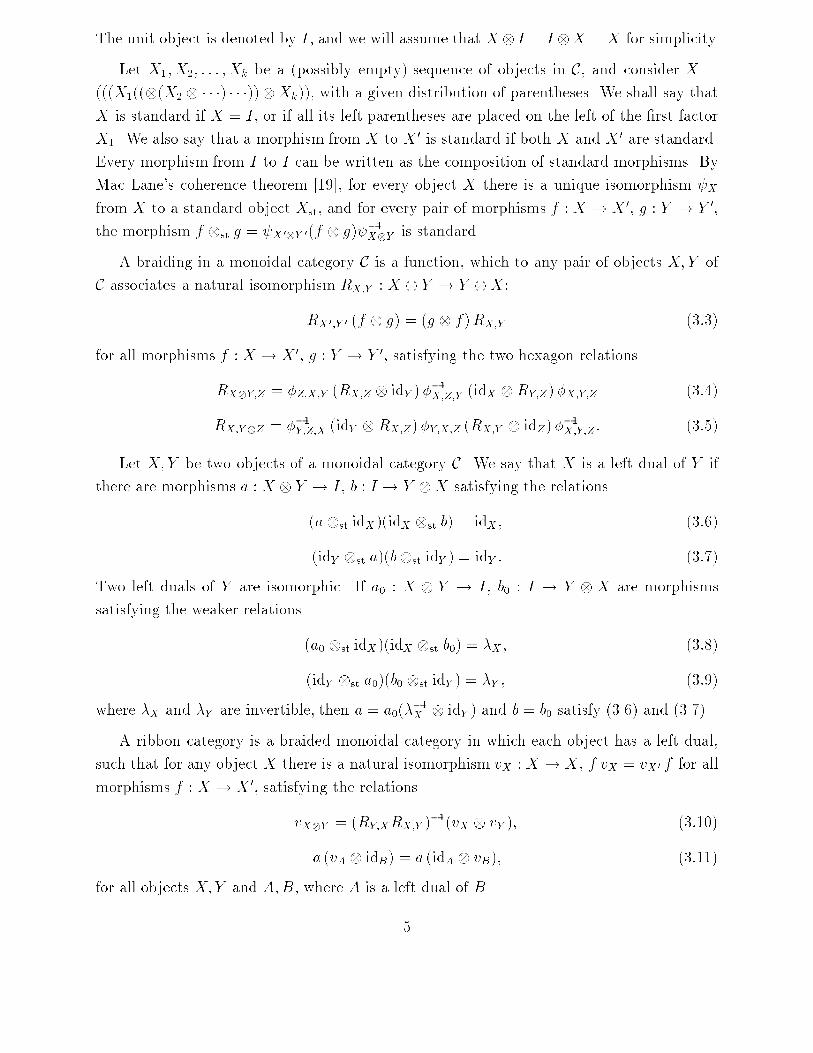
The unit object is denoted by I, and we will assume that X I = I X = X for simplicity.Let X1;X2; : : : ;Xk be a (possibly empty) sequence of objects in C, and consider X =(((X1(((X2 � � �) � � �))Xk)), with a given distribution of parentheses. We shall say thatX is standard if X = I, or if all its left parentheses are placed on the left of the �rst factorX1. We also say that a morphism from X to X 0 is standard if both X and X 0 are standard.Every morphism from I to I can be written as the composition of standard morphisms. ByMac Lane's coherence theorem [19], for every object X there is a unique isomorphism Xfrom X to a standard object Xst, and for every pair of morphisms f : X ! X 0, g : Y ! Y 0,the morphism f st g = X 0Y 0(f g) �1XY is standard.A braiding in a monoidal category C is a function, which to any pair of objects X;Y ofC associates a natural isomorphism RX;Y : X Y ! Y X:RX 0;Y 0 (f g) = (g f)RX;Y (3:3)for all morphisms f : X ! X 0, g : Y ! Y 0, satisfying the two hexagon relationsRXY;Z = �Z;X;Y (RX;Z idY )��1X;Z;Y (idX RY;Z)�X;Y;Z (3:4)RX;YZ = ��1Y;Z;X (idY RX;Z)�Y;X;Z (RX;Y idZ)��1X;Y;Z: (3:5)Let X;Y be two objects of a monoidal category C. We say that X is a left dual of Y ifthere are morphisms a : X Y ! I, b : I ! Y X satisfying the relations(ast idX)(idX st b) = idX ; (3:6)(idY st a)(bst idY ) = idY : (3:7)Two left duals of Y are isomorphic. If a0 : X Y ! I, b0 : I ! Y X are morphismssatisfying the weaker relations (a0 st idX)(idX st b0) = �X ; (3:8)(idY st a0)(b0 st idY ) = �Y ; (3:9)where �X and �Y are invertible, then a = a0(��1X idY ) and b = b0 satisfy (3.6) and (3.7).A ribbon category is a braided monoidal category in which each object has a left dual,such that for any object X there is a natural isomorphism vX : X ! X, f vX = vX 0 f for allmorphisms f : X ! X 0, satisfying the relationsvXY = (RY;XRX;Y )�1(vX vY ); (3:10)a (vA idB) = a (idA vB); (3:11)for all objects X;Y and A;B, where A is a left dual of B.5

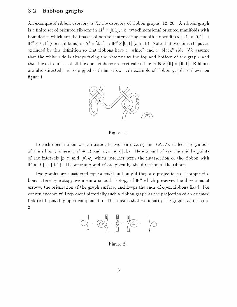
3.2 Ribbon graphsAn example of ribbon category is R, the category of ribbon graphs [12, 20]. A ribbon graphis a �nite set of oriented ribbons in IR2� [0; 1], i.e. two-dimensional oriented manifolds withboundaries which are the images of non self-intersecting smooth embeddings [0; 1]� [0; 1]!IR2� [0; 1] (open ribbons) or S1� [0; 1]! IR2� [0; 1] (annuli). Note that Moebius strips areexcluded by this de�nition so that ribbons have a \white" and a \black" side. We assumethat the white side is always facing the observer at the top and bottom of the graph, andthat the extremities of all the open ribbons are vertical and lie in IR�f0g�f0; 1g. Ribbonsare also directed, i.e. equipped with an arrow. An example of ribbon graph is shown on�gure 1.Figure 1:To each open ribbon we can associate two pairs hx; �i and hx0; �0i, called the symbolsof the ribbon, where x; x0 2 IR and �;�0 2 f"; #g. Here x and x0 are the middle pointsof the intervals [p; q] and [p0; q0] which together form the intersection of the ribbon withIR� f0g � f0; 1g. The arrows � and �0 are given by the direction of the ribbon.Two graphs are considered equivalent if and only if they are projections of isotopic rib-bons. Here by isotopy we mean a smooth isotopy of IR3 which preserves the directions ofarrows, the orientation of the graph surface, and keeps the ends of open ribbons �xed. Forconvenience we will represent pictorially such a ribbon graph as the projection of an orientedlink (with possibly open components). This means that we identify the graphs as in �gure2.

~ ~ ~ ~ Figure 2:6

The objects of R are words w (formal non-associative expressions) of the form((((e12((e22 � � �)) � � �)2ek))) (3:12)where each letter ei, i = 1; : : : ; k is a pair hxi; �ii with xi 2 IR and �i 2 f"; #g. The productof two words w, w0 is w2w0. The unit object is the empty word ;.A morphism w ! w0 in R is a ribbon graph equipped with an assignment of two wordsw and w0, such that the letters of w (w0) are the symbols of the extremities of open ribbonsat the bottom (top). Thus w or w0 = ; if the graph has no extremities of open ribbonsat the bottom or the top. A graph with no open ribbons is called a closed graph. Theclosed graphs are the morphisms from ; to ;. Note that a closed graph de�nes a framedlink, and vice-versa. The tensor product of two graphs C : w ! w0, C 0 : x ! x0, denotedC2C 0 : w2x! w02x0, is de�ned by placing them side by side, as in �gure 3.C' C

. . .

. . . . . .

. . . ...

... ...

... = Figure 3:It will be important for us that every closed graph is a composition of elementary standardgraphs X�i;n, Ti;n and Si;n (�g. 4, 5, 6, 7).

1 i ni+1Figure 4: X+i;nThe morphism �w;w0 ;w00 is shown on �gure 8, the braiding Rw;w0 on �gure 9. A fat linestands for a number of thin parallel lines close to each other representing a word. The leftdual of the word w is the word w0 obtained by reversing the order of the letters and theparentheses, i.e. reading w from right to left, and then reversing the direction of the arrows7

1 i ni+1Figure 5: X�i;n1 ni-1 i+2Figure 6: Ti;n1 ni i+1Figure 7: Si;n8

of each letter. The morphisms a : w02w! ; and b : ; ! w2w0 are shown on �gure 10. Therelations (3.6) and (3.7) are translated on �gure 11. The morphism vw and its inverse aregiven on �gure 12.ω ω'

ω ω')

ω''

(

(

Φ ω ω'

ω''

ω'')

= Figure 8:ω'

R ωω ' =

ω' ω

ω Figure 9:ω ω'

b =

ω ω'

a = Figure 10:3.3 Tensor categoriesLet K be a �eld of characteristic 0. A tensor category T is a strict monoidal category, i.e.� = id, such that for all objects X;Y the morphisms X ! Y form a K-vector space and9

= =

ω

ω ω

ω

ω

ω Figure 11:ϖ

ω

v = ϖ v -1 =

ω

ω ω Figure 12:10

the tensor product of morphisms f g is bilinear, equipped with a symmetric braiding �(�Y;X = ��1X;Y ), and in which every object has a left dual.An in�nitesimal braiding t in T is a function which to any pair X;Y of objects associatesa natural morphism tX;Y : X Y ! X Y satisfying�X;Y tX;Y = tY;X �X;Y ; (3:13)tXY;Z = idX tY;Z + p�1(tX;Z idY )p; (3:14)where p = idX�Y;Z. For example, if G is a �nite-dimensional semisimple Lie algebra, thereis an in�nitesimal braiding in the category of �nite-dimensional G-modules given bytX;Y =Xa (ea)X (ea)Y ; (3:15)where feag is a basis of G, feag is the dual basis with respect to the Killing form, and (ea)Xdenotes the action of ea on X.Let Bm be the associative graded algebra over K with generators tij = tji, i 6= j, i; j 2f1; : : : ;mg of degree 1, and relations [tij; tik + tjk] = 0; (3:16)[tij; tkl] = 0; (3:17)where i; j; k; l are distinct. Denote bydBm the completion with respect to the topology de�nedby the gradation. Similarly, let F2 be the free associative graded algebra on two generatorsA1; A2 of degree 1, and let cF2 be its completion. A Drinfeld series, or associator, is a formalnon-commutative series �(A1; A2) 2 cF2 satisfying�(A1; A2) = �(A2; A1)�1; (3:18)�(t12; t23 + t34)�(t13 + t23; t34) = �(t23; t34)�(t12 + t13; t24 + t34)�(t12; t23); (3:19)exp 12(t13 + t23) = �(t13; t12) exp 12(t13)�(t13; t23)�1 exp 12(t23)�(t12; t23); (3:20)where the last two relations hold in cB4. Drinfeld has shown [17, 18] that such series existfor all K, in particular K = Q. For K = C he gave an explicit construction of a solution�KZ using the properties of the Knizhnik-Zamolodchikov equations: �KZ(A1; A2) = G�12 G1,where G1; G2 2 cF2 are two solutions of the di�erential equationG0(x) = 12�i �A1x + A2x� 1�G(x) (3:21)de�ned in 0 < x < 1 with the asymptotic behaviour G1(x) � xA1=2�i for x ! 0 andG2(x) � (1 � x)A2=2�i for x ! 1. The coe�cients of �KZ are given by generalizations ofRiemann's � function [15]. 11

Note that cF2 becomes a topological Hopf algebra with the comultiplication de�ned by�(Ai) = Ai 1 + 1 Ai, i = 1; 2. Let L be the Lie algebra of primitive elements incF2, and let L0 = [L;L] be the derived subalgebra. Then log �KZ(A1; A2) 2 L0, and if�(A1; A2) is a solution of (3.18-3.20) of the form expP (A1; A2) with P (A1; A2) 2 L, thenthe decomposition P = Pn�1 Pn into homogeneous elements Pn of degree n satis�es P1 = 0,i.e. P 2 L0, P2 = (1=24)[A1; A2], P3 = a3([A1; [A1; A2]] � [A2; [A2; A1]]), where a3 2 K isarbitrary.Given any tensor category T with an in�nitesimal braiding t, we can construct a ribboncategory T [[h]], as follows. It has the same objects as T , but a morphism X ! Y in T [[h]]is a formal series Pn�0 fnhn, where fn : X ! Y is a morphism of T . The tensor product ofobjects is the same as in T , and the tensor product of morphisms is the extension to K[[h]]of the one in T , with the non-trivial associator�X;Y;Z = �(htX;Y ; htY;Z): (3:22)To deform the duality, one needs the remark after (3.8), (3.9) with a0, b0 the duality mor-phisms of the strict category T . The morphisms �X and �Y are invertible, for any formalpower series in h beginning with 1 is invertible. The braiding is given byRX;Y = �X;Y exp h2 tX;Y ! ; (3:23)and the ribbon structure by vX = exp �h2 X! ; (3:24)where X = �(idX a tA;X)(b idX) plays the role of the quadratic Casimir operator andA is a left dual of X. By the additivity property (3.14) of t, we have2 tX;Y = XY � X idY � idX Y ; (3:25)and the relation (3.10) follows.Now we can de�ne a generalized Reshetikhin-Turaev functor F : R ! T [[h]], whichrestricted to closed ribbon graphs gives an invariant of oriented framed links. We choose �rsta �xed object X# in T [[h]], and a left dual X" of X#. We put F (hx; #i) = X#, F (hx; "i) = X"and extend the de�nition of F to all objects of R by requiring F (w2w0) = F (w) F (w0).To de�ne F on morphisms, we require that F preserves �, the braiding R, the family ofmorphisms a and b which de�ne duality, and the ribbon structure v.12

4 The category of diagramsA chord diagram D is a pair (X;C), where X is a set of lines and circles and C is a set ofchords connecting pairs of points in X. The precise de�nition is as follows: X is a compactoriented, piecewise smooth one-dimensional submanifold of IR2� [0; 1] = f(x; y; t)j0 � t � 1gsuch that:(i) its connected components Xj , j = 1; : : : ;m, are homeomorphic to [0; 1] or S1,(ii) @X = N0 [ N1, where Ni = @X \ Ei, Ei = f(x; 0; i) jx 2 IRg,(iii) for each x 2 Ni, i = 0; 1, the function t restricted to the tangent line to X at x is notconstant, i.e. the tangent line is not horizontal.A chord on X is a subset fx; yg � Xn@X of two elements x 6= y, and C is a �nite set ofdisjoint chords onX, possibly empty. X is called the support of the diagram. If Card(C) = nwe shall say that the diagram D = (X;C) is of order n. A point x 2 X such that fx; yg 2 Cfor some y 2 X is called a vertex. Chord diagrams are represented as in �g. 13.Figure 13:We identify two diagrams if they are related by a di�eomorphism which sends the linesE0 and E1 into themselves and conserves the orientation of X, E0 and E1. Note that inparticular this implies that over and under-crossings are identi�ed in chord diagrams, see�g. 14.

= Figure 14:13

Let K be a �eld of characteristic 0, and D(n) be the K-vector space spanned by thediagrams of order n. The space of Bar-Natan diagrams of order n is B(n) = D(n)=R(n),where R(n) is the subspace of D(n) spanned by the linear combinations of 4 diagrams de�nedin �g. 15. Note that the 4 terms of �g. 15 stand for arbitrary diagrams D1; : : : ;D4 whichare equal except for the parts shown there.= 0- +- Figure 15:Now we are ready to de�ne the category DK of diagrams. Its objects are �nite sequencesS = (�1; �2; : : : ; �k), where �j 2 f"; #g, j = 1; : : : ; k, including the empty sequence ;. ABar-Natan diagram with support X is a morphism from S0 to S1, the Si being de�ned asfollows: use the fact that Ei is an ordered set, to build a sequence of unit tangent vectors~Si = (u1; u2; : : : ; uk), where u1 is the tangent vector to X at the smallest x 2 Ni, u2 is thenext tangent vector to X along Ei, and so on. Then Si is given by the projection of ~Si onthe vertical axis t.The composition of morphisms is de�ned as follows: if b : S0 ! S1 and b0 : S00 ! S01are morphisms with S1 = S00 de�ned by the diagrams (X;C) and (X 0; C 0), we �rst translate(X 0; C 0) in IR2 � [1; 2], then glue N1 to N 00 and �nally scale t for 0 � t � 2 by a factor1=2. This de�nes a chord diagram (X 00; C 00) and a morphism b00 = b0 b : S0 ! S01. This isillustrated on �g. 16.

b’. b =

b’= b =

Figure 16:14

The identity morphism is represented by the diagram of order 0 on �g. 17.Figure 17:This category of diagrams DK is a tensor category. The monoidal structure is de�nedon objects as concatenation of sequences, the unit object being ;. For morphisms b b0is juxtaposition, see �g. 18. The symmetric braiding �S;S0 is given by either one of thediagrams of �g. 14.

= Figure 18:For �;�0 2 f"; #g, let �;�0 be the diagram of �g. 19, with � and �0 given by theorientations (not shown on the �gure) of the two lines. The category DK has an in�nitesimalbraiding t de�ned by t�;�0 = ��;�0, where the sign is + or - according to whether � = �0 ornot. We denote by tij, with i; j 2 f1; : : : ; ng any diagram of degree one, whose support hasn connected components which are parallel vertical lines, such that it reduces to a diagramt�;�0 if all lines but those labeled i and j are deleted.Figure 19:For any tensor category T over K with an in�nitesimal braiding t, and any object X#in T with a left dual X", there is a functor of tensor categories WT : DK ! T de�ned byWT (#) = X#, WT (") = X" and WT (t�;�0) = tX�;X�0 , for �;�0 2 f"; #g. This functor de�nes a15

weight system (Feynman rules) on DK . The Reshetikhin-Turaev functor FU : R ! DK [[h]]de�ned in the previous section is called the universal Vassiliev invariant. For any Reshetikhin-Turaev functor F : R ! T [[h]], F = WT � FU , because DK is a free [19] tensor categorywith in�nitesimal braiding.From several sources [18, 20, 13] we can extract the next theorem, which enables thecomputation of FU(L) for any framed link (closed ribbon graph) L. Before stating it, weneed a de�nition: let idk be the identity morphism of an object S in DK which is a sequenceof k arrows. We consider idk as a standard morphism in DK [[h]]. For any morphism f inDK [[h]], de�ne f(k) recursively by f(0) = f , f(k) = f(k�1) id1, and put fj;k = (idj f)(k).Theorem 1 The functor FU takes on the elementary standard ribbon graphs the valuesFU(X�i;n) = (�(i))�1�i;i+1 exp(�h2 ti;i+1)�(i) (4.1)FU(Ti;n) = ai�1;n�i�1 �(i) (4.2)FU(Ti;n) = (�(i))�1 bi�1;n�i�1 (4.3)where �(i) = �(h i�1Xj=1 tji; hti;i+1): (4:4)In fact FU depends on the choice of a solution � to (3.18-3.20). What is remarkable is thatfor closed graphs L (framed links), FU(L) is independent of the choice of � [21]. This impliesthat the coe�cients of the universal Vassiliev invariant of links are rational.We denote by A(X) the space of all chord diagrams with support X. The space A =A(S1) has the structure of a commutative algebra, with the multiplication de�ned by meansof the connected sum of the two circles [9, 10]. If X has m connected components Xj,1 � j � m, then for each value of j we can de�ne an A-module Aj(X), which is isomorphicto A(X) as a vector space, and for which the action of A is given by the connected sumS1#Xj, where S1 is the circle of A = A(S1). This is illustrated in �g. 20. The 4-termrelation of �g. 15 implies that the result is independent of the point of insertion of the circle.For further convenience we de�ne � 2 A as the unique chord diagram on S1 of degree 1,shown on �g. 21.5 The Kontsevich integralLet G be a standard ribbon graph, i.e. a morphism of R from w to w0, where w and w0are two standard words. Remember that G is an equivalence class of ribbons which are16

= =. Figure 20:Figure 21:related by an isotopy of C � [0; 1] = f(z; t) j 0 � t � 1g. We choose a particular elementG in this class, such that t is a Morse function on G, i.e. for a given value t = t0 there isat most one extremum of G. Each connected component Gj is the image of an embedding� : G0j � [0; 1] ! C � [0; 1], where G0j = [0; 1] or S1. We assume that G is contained in theplane Im(z) = 0 except for small neighbourhoods around the crossings of �gs. 4 and 5, whereonly the framing vector �(x; 1)� �(x; 0) is contained in the plane Im(z) = 0. In other words,we use the blackboard framing. Let Xj(G) be the curve �(G0j �f0g), X(G) = Sj Xj(G). Leth be a formal variable, �h = h(2�i)�1, � > 0 andZ�(G) = 1Xn=0 �hn Z tmin<t1<���<tn<tmaxjzi�z0ij>� XpairingsP=f(zi;z0i)g(�1)#P"D(G; P ) nYi=1 dzi � dz0izi � z0i (5:1)Here tmin and tmax are the minimal and maximal value of t on X(G), a pairing P is a choiceof n unordered pairs (zi; z0i), such that for 1 � i � n, (zi; ti) and (z0i; ti) are distinct pointson X(G), #P" is the number of vertices (zi, z0i) of P at which X(G) is oriented upwards.The coordinates zi and z0i are considered as functions of ti, and integration is over the subsetof the n-simplex tmin < t1 < � � � < tn < tmax de�ned by the conditions jzi(ti) � z0i(ti)j > �.D(G; P ) is the chord diagram of degree n with the support X(G) and the set of chords Cde�ned by the pairing P . (�g.22).Now we de�ne the regularized Kontsevich integral as:Z(G) = lim�!0 mYj=1 ��h(n+j �n�j )�j � Z�(G) (5:2)where n�j are the number of critical points (maxima and minima) of the Morse function ton the component Xj(G), and �j denotes the diagram � acting on the latter. (Notice that17

t3

t2t1

x

y Figure 22:n+j �n�j = 0 if j corresponds to a circle.) Later we will show that a slightly modi�ed versionof Z(G) is invariant under isotopies of ribbons.We recover the usual de�nition of the Kontsevich invariant if we impose the additionalrelation � = 0, i.e if every diagram having an isolated cord is set equal to zero. Thiscondition implements the framing independence in the original Kontsevich integral [10, 9].Theorem 2 The regularized Konsevitch integral is well-de�ned and multiplicative:Z(G G0) = Z(G)Z(G0): (5:3)Proof. A pairing P 00 of G G0 can be partitioned into a disjoint union of pairings P , P 0 of Gand G0, such that D(G G0; P 00) = D(G; P )D(G0; P 0). Letf = (�1)#P"D(G G0; P 00) nYi=1 fi(ti); (5:4)where fi(ti) = 8<: @@ti log(zi � z0i); if jzi � z0ij > �0 otherwise: (5:5)The formulaZa<t1<:::<tn<b dt1 : : : dtn f = nXp=0 Za<t1<:::<tp<c dt1 : : : dtp Zc<tp+1<:::<tn<b dtp+1 : : : dtn f (5:6)18

implies that Z�(G G0) = Z�(G)Z�(G0). The action of each factor �j in (5.2) through theconnected sum is independent of its point of insertion on the diagram D(G; P ), thus we can"move" it along the support until it reaches an extremum. By the de�nition of the Morsefunction t we can decompose G into a product of standard graphs each of which containsonly one extremum. Therefore the theorem is proved if we can show that Z converges forsuch a graph. This is done in lemma 1 below. 2The main ingredient in the construction of the Kontsevich invariant Z(G), as we nowexplain, appears when G contains no extremum, so that it becomes a braid. Consider a path : [0; 1]! Vm, where Vm = f(z1; : : : ; zm) 2Cm j zi 6= zj; i 6= jg: (5:7)Let i(t) = zi(t), t 2 [0; 1] be the i-th component of this path. Construct a ribbon graph G out of , such that its i-th connected component G i : [0; 1]� [0; 1]!C� [0; 1] is given byG i (t; u) = ( i(t) + u�; t); (5:8)where u 2 [0; 1], and � 2 IR is a constant.Suppose �rst that is a closed path. Let ij be the chord diagram of degree one, withsupport Sjf( j(t); t) j t 2 [0; 1]g, and its chord connecting the components labeled by i andj. De�ne the abstract Knizhnik-Zamolodchikov connection with values in the algebra Bmgenerated by the ij, 1 � i; j � m, as the 1-form on Vm:! = �hXi<j sisjij dzi � dzjzi � zj (5:9)where si = �1 according to whether the orientation of the i-th component is downwards orupwards. It is easy to see that Z(G ) = �exp Z 10 �!: (5:10)Let us quickly recall some well-known properties [22] of Z(G ). Let 0 be another closedpath in Vm, with 0(1) = (0), and let 0 � denote their product. Then we have Z(G 0� ) =Z(G 0)Z(G ). Set tij = sisjij. The four-term relation satis�ed by diagrams (�g. 15)means that the generators tij of Bm satisfy (3.16). The KZ connection ! is closed, d! = 0,and the relation (3.16) is equivalent to !^! = 0, so that ! is at: F! = d!+!^! = 0. Thisimplies that Z(G ) only depends on the homotopy class of , so that the map 7! Z(G )de�nes a representation �1(Vm; �) ! Bm, where � = (0) = (1) is a �xed basepoint. Since�1(Vm; �) is the pure braid group on m strands Pm [23], the Kontsevich integral Z(G ) givesa representation of Pm in the algebra Bm. 19

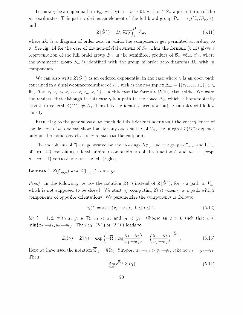
Let now be an open path in Vm, with (1) = � � (0), with � 2 Sm a permutation of them coordinates. This path de�nes an element of the full braid group Bm = �1(Vm=Sm; �),and Z(G ) = D� �exp Z 10 �!; (5:11)where D� is a diagram of order zero in which the components get permuted according to�. See �g. 14 for the case of the non-trivial element of S2. Thus the formula (5.11) gives arepresentation of the full braid group Bm in the semidirect product of Bm with Sm, wherethe symmetric group Sm is identi�ed with the group of order zero diagrams D� with mcomponents.We can also write Z(G ) as an ordered exponential in the case where is an open pathcontained in a simply-connected subset of Vm, such as them-simplex�m = f(z1; : : : ; zm) j zi 2IR ; 0 < z1 < z2 < � � � < zm < 1g. In this case the formula (5.10) also holds. We warnthe readers, that although in this case is a path in the space �m which is homotopicallytrivial, in general Z(G ) 6= D1 (here 1 is the identity permutation). Examples will followshortly.Returning to the general case, to conclude this brief reminder about the consequences ofthe atness of !, one can show that for any open path of Vm, the integral Z(G ) dependsonly on the homotopy class of relative to the endpoints.The morphisms of R are generated by the crossings X�m;n and the graphs Tm;n and Sm;nof �gs. 4-7 containing a local minimum or maximum of the function t, and m � 1 (resp.n�m� 1) vertical lines on the left (right).Lemma 1 Z(Tm;n) and Z(Sm;n) converge.Proof. In the following, we use the notation Z( ) instead of Z(G ), for a path in Vm,which is not supposed to be closed. We start by computing Z( ) when is a path with 2components of opposite orientations. We parametrize the components as follows:zi(t) = xi + (yi � xi)t; 0 � t � 1; (5:12)for i = 1; 2, with xi; yi 2 IR, x1 < x2 and y1 < y2. Choose an � > 0 such that � �minfx2 � x1; y2 � y1g. Then eq. (5.1) or (5.10) leads toZ�( ) = Z( ) = exp��12 log y1 � y2x1 � x2� = � y1 � y2x1 � x2��12 : (5:13)Here we have used the notation ij = �hij. Suppose x2�x1 > y2�y1, take now � = y2�y1.Then lim�!0 �12 Z�( ) (5:14)20

exists, and the same is true in the other case � = x2 � x1 < y2 � y1, namelylim�!0Z�( ) ��12 : (5:15)Consider now m;n, the same path with m � 1 (resp. n � m � 1) vertical lines on the left(right) and the two center lines as in . The parametrization we choose is zi = const 2 IRfor i 6= m;m+ 1 and zi as in (5.12) for i = m;m+ 1. We will now prove that the limitslim�!0 �m;m+1 Z�( m;n) (5:16)and lim�!0Z�( m;n) ��m;m+1 (5:17)exist, where � = minfxm+1�xm; ym+1� ymg, and maxfxm+1�xm; ym+1� ymg is �xed. TheKZ connection can be written as! = �m;m+1 dzm � dzm+1zm � zm+1 + !0; (5:18)where !0 = Xk 6=m;m+1 smsk m;k dzmzm � zk � m+1;k dzm+1zm+1 � zk! : (5:19)Using the factorization formula (2.10), we �ndZ( m;n) = g(ym � ym+1) �exp Z 10 �g(zm � zm+1)�1!0 g(zm � zm+1)� ; (5:20)where g(z) = zxm � xm+1!�m;m+1 : (5:21)Therefore, the relation (3.16) implies thatg(ym � ym+1)�1Z( m;n) = �exp Z 10 (!0 + !00) (5:22)where!00 = 1Xp=1 1p! logp zm � zm+1xm � xm+1! adp(m;m+1) Xk 6=m;m+1 smskmk dzmzm � zk � dzm+1zm+1 � zk! ;(5:23)and to prove that (5.16) exists, it is enough to show thatIp = Z 10 dt logp(zm+1 � zm) _zmzm � zk � _zm+1zm+1 � zk! (5:24)21

converges when ym ! ym+1, for any positive integer p. Here we have adopted the notationdz=dt = _z. WritingIp = Z 10 dt logp(zm+1 � zm) _zm(zm+1 � zm)(zm � zk)(zm+1 � zk) � _zm+1 � _zmzm+1 � zk ! ; (5:25)and noting that (zm+1 � zm) logp(zm+1 � zm) ! 0 as zm+1 � zm ! 0, we see that the �rstterm converges. As for the second term, we put( _zm+1 � _zm) logp(zm+1 � zm) = ddtFp(zm+1 � zm); (5:26)where Fp(z) = Z zz0 dx logp x; (5:27)and observe that the function Fp(z) is de�ned at z = 0. Thus, integrating by parts provesthat Z 10 dt dFp(zm+1 � zm)=dtzm+1 � zk (5:28)converges. This concludes the proof that the limit (5.16) exists. Similarly, one can show theexistence of (5.17).Notice that since the KZ connection is at, (5.16) and (5.17) do not depend on the detailsof the path m;n, but only on its endpoints. From the de�nition of the regularized integral(5.2), we see that for � = minfxm+1� xm; ym+1 � ymg, keeping maxfxm+1 � xm; ym+1� ymg�xed, Z(Tm;n) = lim�!0 T0m;n �m;m+1 Z�( m;n) = lim�!0 (��h�m � T0m;n)Z�( m;n); (5:29)Z(Sm;n) = lim�!0 Z�( m;n) ��m;m+1 S0m;n = lim�!0 Z�( m;n) (���h�m � S0m;n); (5:30)where T0m;n and S0m;n are diagrams in DK of order zero with supports given by Tm;n, Sm;n,such that the extremities of the line containing the maximum (resp. minimum) are ym andym+1 (xm and xm+1). 2Now we want to show that (5.29) and (5.30) are independent of the location of theextremum. We give the proof for a maximum. For this we proceed in two steps. The �rststep is illustrated in �g. 23. The �gure represents the expression T0m;n �m;m+1 Z�( m;n).Using atness one replaces m;n by a path whose top part T has the lines zm and zm+1satisfying jzm�zm+1j = �. In the second step, we show that the contribution of this top partis trivial: Z(T ) = T , the diagram with no chords, therefore T can be erased. To prove thatthe second step is justi�ed, we observe that if there exists a constant C > 0 independent of� such that jzm � zkj � C, for all k 6= m;m+ 1, then the integral Ip corresponding to T {de�ned in (5.24) and written conveniently in (5.25) { tends to zero when � goes to zero.22

Note that these arguments apply not only to Tm;n, but to all the graphs A2stT1;22stB,where A, B are arbitrary standard ribbon graphs. They show that the maxima and minimacan be moved freely without changing the value of Z, except for the two con�gurations shownon �g. 24 and 25, where there is no constant C satisfying the conditions. In the case of �g.24 this is not a failure, but a nice feature of Z, since we want to get an invariant of ribbons.One cannot remove the parts of a ribbon graph which look like �g. 25 without changing thevalue of Z, because the diagrams T01;2 and S01;2 are not the morphisms a and b of DK[[h]],they satisfy only the weak properties (3.8) and (3.9). However, if we de�ne Z(G) byZ(Tm;n) = ��1 � Z(Tm;n); (5:31)where � = Z(U) and U is the diagram of �g. 26, acting on the component of Tm;n carryingthe maximum, and Z(G) = Z(G) for the other elementary graphs G, then Z is invariantunder insertion or removal of the subgraph of �g. 25. The atness of the KZ connectionimplies that Z is invariant under an isotopy which �xes the extrema. Thus we get:Theorem 3 Z(G) is an isotopy invariant of ribbon graphs.ε ε

d d

ε Figure 23:Figure 24:23

Figure 25:Figure 26:6 The distancing operatorIn this section we introduce the distancing operator, which is the renormalized Kontsevichintegral of a trivial braid with a pair of consecutive strands moving away from each other toin�nity. Let a 2 IR, � > 0. We consider a path �(n)i : [0; 1]! �n, such that�(n)i (1) = (z1; : : : ; zn);�(n)i (0) = (z1 � a; : : : ; zi � a; zi+1 + � � a; : : : ; zn + �� a): (6.1)(The strands i and i + 1 are moving away from each other.) Due to the zero curvaturecondition satis�ed by the KZ connection and the fact that �n is simply-connected we canchoose any path with these endpoints to calculate Z(�(n)i ). Let us take the following one:�(n)i (t) = 8<: zj � a(1� t) 1 � j � izj + (1� t)(�� a) i+ 1 � j � n; � > 0: (6:2)It is useful to remark that Z(�(n)i ) does not depend on the global translation a because the KZconnection depends only on the di�erences zj(t)� zi(t). We put g(n)i (�; z1; : : : ; zn) = Z(�(n)i )and in the following we will not mention the arguments (z1; : : : ; zn) if there is no ambiguity.Using the de�nition of the Kontsevich integral we have:g(n)i (�) = �exp(�h Z 10 dt !(t)); (6:3)where !(t) = iXj=1 nXk=i+1 �tjk(t� 1)� + zj � zk (6:4)24

The distancing operator is obtained by sending � to in�nity, but to do this a regularizationis needed.Theorem 4 Set X(n)i =Pij=1Pnk=i+1 tjk.1. The distancing operatorD(n)i (z1; : : : ; zn) = lim�!+1 g(n)i (�)��hX(n)i (6:5)is a well-de�ned function on Vn with values in Bn[[h]], the algebra of formal power series inh with coe�cients in Bn.2. It has the asymptotic behaviour D(n)i � (zn � z1)��hX(n)i in the region8<: zn � z1 >> zn � zk; k > izn � z1 >> zj � z1; j � i : (6:6)3. It satis�es the di�erential equations@D(n)i@zj = �h0B@ nXk=1k 6=j tjkzj � zk1CAD(n)i � �hD(n)i K(n)ij ; (6:7)where K(n)ij = 8><>: Pik=1k 6=j tjkzj�zk ; j � iPnk=i+1k 6=j tjkzj�zk ; j > i: (6:8)Proof. 1. We factorize from g(n)i (�) �exp(�h Z 10 dt �X(n)i(t� 1)� + z1 � zn ) = � zn � z1�+ zn � z1��hX(n)i : (6:9)Thus, using (2.11) and performing the change of variables x = �(1 � t)=(zn � z1) we get:g(n)i (�) = �exp(�h Z 0�zn�z1dx ~!(x)) � zn � z1�+ zn � z1��hX(n)i ; (6:10)with ~!(x) = (1 + x)��hX(n)i 0B@ X1�j�ii+1�k�n tkj(1 � ukj)(x+ ukj)(1 + x)1CA (1 + x)�hX(n)i (6:11)and ukj = (zk � zj)=(zn � z1). Since~!(x) = +1Xp=0 �hpp! 0B@ X1�j�ii+1�k�n adp(X(n)i ) � tkj1CA (1� ukj) logp(1 + x)(x+ ukj)(x+ 1) ; (6:12)25

and the integral Z +10 dx logp(1 + x)(x+ ukj)(1 + x) (6:13)converges, we deduce that �exp(�h Z 0+1dx~!(x)) (6:14)converges as a formal series in h, which means that all the integrals appearing in its expansionconverge.2. The asymptotic region (6.6) is de�ned by ukj = 1; 1 � j � i; i+1 � k � n. In this region~!(x) = 0, thus D(n)i (zn � z1)��hX(n)i = 1.3. The formula (2.8) yields:@@zj g(n)i (�) = �h Z 10 dt h(1; t) @@zj 0B@� X1�l�ii+1�k�n �tlk�(1 � t) + zk � zl1CA h(t; 0); (6:15)where h(x; y) = �exp(�h Z xy du!(u)): (6:16)Using @@zj 0B@ X1�l�ii+1�k�n � tlk�(1 � t) + zk � zl1CA = @@t 0@ Xi+1�k�n tjk�(1 � t) + zk � zj1A (6:17)if j � i, and integrating by parts over t, the r.h.s. of (6.15) becomes:�h Xi+1�k�n tjkzj � zk g(n)i (�)� �hg(n)i (�) Xi+1�k�n tjk� + zj � zk (6.18)��h Z 10 dt h(1; t) 2664 Xi+1�k�n tjk�(1 � t) + zk � zj ; X1�j0�ii+1�k0�n �tj0k0�(1 � t) + zk0 � zj0 3775 h(t; 0):Using in the second term the classical Yang-Baxter equation:" tjkzj � zk ; tj0kzj0 � zk #+ " tjj0zj � zj0 ; tjkzj � zk + tj0kzj0 � zk # = 0; (6:19)and again the derivation property (2.8) we get:@@zj g(n)i (�) = �h0B@ nXk=1k 6=j tjkzj � zk1CA g(n)i (�)� �hg(n)i (�)0BB@ iXj0=1j0 6=j tjj0zj � zj0 + nXk=i+1 tjkzj � zk � �1CCA : (6:20)26

Nowmultiply on the right this equality by ��hX(n)i , and notice that [X(n)i ; tjj0] = 0, 1 � j; j0 � iand lim�!1 ���hX(n)i nXk=i+1 tjkzj � zk � � ��hX(n)i = 0: (6:21)Here the limit means that each term in the h expansion tends to zero. This proves part 3 ofthe theorem for 1 � j � i (the proof for the case i+ 1 � j � n is identical). 2Remark. The distancing operator is equivalently de�ned as being the solution of thedi�erential equations (6.7) on Vn, satisfying the asymptotic conditions (6.6).Let A be a standard ribbon graph such that its top (resp. bottom) endpoints are(z1; : : : ; zi) 2 �i (resp. (z01; : : : ; z0p) 2 �p), and let B be a standard ribbon graph suchthat its top (resp. bottom) endpoints are (zi+1; : : : ; zn) 2 �n�i (resp. (z0p+1; : : : ; z0q) 2 �q�p).(Here \endpoint" really means the middle point of the intersection of an open ribbon withIR� f0g � f0; 1g.) We put these graphs side by side such that the top (resp. bottom) end-points (z1; : : : ; zi; zi+1; : : : ; zn) (resp. (z01; : : : ; z0p; z0p+1; : : : ; z0q)) of A2B lie in �n (resp. �q).This is always possible up to a global translation of B. The product A2B is not standard.Let A2stB be the same graph as A2B but with the standard arrangement of parentheses.Theorem 5 Z(A2stB) = D(n)i (z1; : : : ; zn) (Z(A) Z(B)) (D(q)p (z01; : : : ; z0q))�1: (6:22)Proof. Let (A2stB)� be the ribbon graph whose top (resp. bottom) endpoints are(z1 � �=2; : : : ; zi � �=2; zi+1 + �=2; : : : ; zn + �=2)( resp: (z01 � �=2; : : : ; z0p � �=2; z0p+1 + �=2; : : : ; z0q + �=2)): (6.23)Then A2stB and �(n)i (z1; : : : ; zn) (A2stB)� (�(q)p (z01; : : : ; z0q))�1 are isotopic ribbon graphs (see�g. 27), where the path �(n)i is de�ned in (6.2), and the same symbol is used here for theassociated standard ribbon graph constructed as in (5.8). We also set (�(n)i )�1(t) = �(n)i (1�t),0 � t � 1.Thus Z(A2stB) = g(n)i (�)Z((A2stB)�)(g(q)p (�))�1 (6.24)= (g(n)i ��hX(n)i )����hX(n)i Z((A2stB)�))��hX(q)p � (g(q)p ��hX(q)p )�1: (6.25)From the de�nition of the regularized Kontsevich integral one sees thatZ((A2stB)�) = Z(A) Z(B) +Xn�1 �hnf(n)(�); (6:26)27

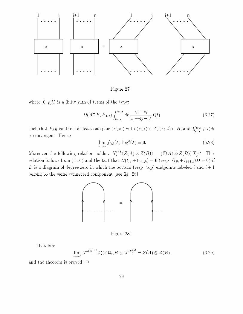
1 i i+1 n 1 i i+1 n

= BABA Figure 27:where f(n)(�) is a �nite sum of terms of the type:D(A2B;PAB) Z tmaxtmin dt _zi � _zjzi � zj + �f(t) (6:27)such that PAB contains at least one pair (zi; zj) with (zi; t) 2 A, (zj; t) 2 B, and R tmaxtmin f(t)dtis convergent. Hence lim�!1 f(n)(�) logp(�) = 0: (6:28)Moreover the following relation holds : X(n)i (Z(A) Z(B)) = (Z(A) Z(B))X(q)p . Thisrelation follows from (3.16) and the fact that D(tik + ti+1;k) = 0 (resp. (tik + ti+1;k)D = 0) ifD is a diagram of degree zero in which the bottom (resp. top) endpoints labeled i and i+ 1belong to the same connected component (see �g. 28).=Figure 28:Therefore lim�!1���hX(n)i Z((A2stB)�)��hX(q)p = Z(A) Z(B); (6:29)and the theorem is proved. 2 28

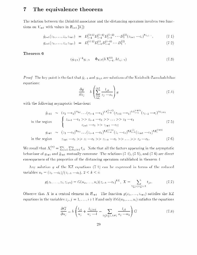
7 The equivalence theoremThe relation between the Drinfeld associator and the distancing operators involves two func-tions on Vi+1 with values in Bi+1[[h]]:~gi+1(z1; : : : ; zi; zi+1) = D(i+1)i�1 D(i�1)i�2 D(i�2)i�3 � � �D(2)1 (zi+1 � zi)�hti;i+1 ; (7.1)gi+1(z1; : : : ; zi; zi+1) = D(i+1)i D(i)i�1D(i�1)i�2 � � �D(2)1 : (7.2)Theorem 6 (~gi+1)�1gi+1 = �KZ(hX(i)i�1; hti;i+1) (7:3)Proof. The key point is the fact that ~gi+1 and gi+1 are solutions of the Knizhnik-Zamolodchikovequations: @g@zj = �h0B@ i+1Xk=1k 6=j tjkzj � zk1CA g (7:4)with the following asymptotic behaviour:~gi+1 � (z2 � z1)�ht12 : : : (zi�1 � z1)�hX(i�1)i�2 (zi+1 � z1)�hX(i+1)i�1 (zi+1 � zi)�hti;i+1in the region 8<: zi+1 � z1 >> zi�1 � z1 >> : : : >> z2 � z1zi+1 � z1 >> zi+1 � zi; (7.5)gi+1 � (z2 � z1)�ht12 : : : (zi�1 � z1)�hX(i�1)i�2 (zi � z1)�hX(i)i�1(zi+1 � z1)�hX(i+1)iin the region zi+1 � z1 >> zi � z1 >> zi�1 � z1 >> : : : >> z2 � z1: (7.6)We recall that X(n)i = Pij=1Pnk=i+1 tjk. Note that all the factors appearing in the asymptoticbehaviour of gi+1 and ~gi+1 mutually commute. The relations (7.4), (7.5), and (7.6) are directconsequences of the properties of the distancing operators established in theorem 4.Any solution g of the KZ equations (7.4) can be expressed in terms of the reducedvariables uk = (zk � z1)=(zi+1 � z1), 2 � k � i:g(z1; : : : ; zi; zi+1) = G(u2; : : : ; ui)(zi+1 � z1)�hX ; X = X1�j<k�i+1 tjk: (7:7)Observe that X is a central element in Bi+1. The function g(z1; : : : ; zi+1) satis�es the KZequations in the variables zj, j = 1; : : : ; i+1 if and only ifG(u2; : : : ; ui) satis�es the equations@G@uj = �h0@tj1uj + tj;i+1uj � 1 + X2�k�i; k 6=j tjkuj � uk1AG (7:8)29

for j = 2; : : : ; i. Now if we set Ui+1 = u��ht122 : : : u��hX(i�1)i�2i�1 Gi+1; (7:9)and the same for ~Ui+1, ~Gi+1, we obtain that Ui+1 and ~Ui+1 are analytic functions in thedomain 1 > ui > ui�1 � ui�2 � : : : � u2 � 0, and they obey the same linear di�erentialequations. Moreover, at the point ui�1 = ui�2 = : : : = u2 = 0 it follows from (7.8) that theysatisfy the equation @U@ui = �h0@X(i)i�1ui + ti;i+1ui � 11AU (7:10)with the asymptotic behaviour: Ui+1 � (ui)�hX(i)i�1 ui ! 0 (7.11)~Ui+1 � (1� ui)�hti;i+1 ui ! 1: (7.12)Thus, at the point ui�1 = ui�2 = : : : = u2 = 0,( ~Ui+1)�1Ui+1 = �KZ(hX(i)i�1; hti;i+1); (7:13)and by the uniqueness of the solution of di�erential equations this equality holds in the wholedomain 1 > ui > ui�1 � ui�2 � : : : � u2 � 0. 2We have seen already in section 3 that any closed ribbon graph is a composition ofelementary standard graphs X�m;n, Tm;n and Sm;n. Recall that T0m;n and S0m;n are diagramsin DK of order zero with supports given by Tm;n, Sm;n. Put �(i)KZ = �KZ(hX(i)i�1; hti;i+1).Theorem 7 The value of the regularized Kontsevich integral on the elementary graphs is:Z(X�i;n) = gn(�(i)KZ)�1 exp(�h2 ti;i+1)D�i;i+1 �(i)KZ g�1n (7.14)Z(Ti;n) = gn�2 �T0i;n�(i)KZ� g�1n (7.15)Z(Si;n) = gn �(�(i)KZ)�1S0i;n� g�1n�2: (7.16)Comparing with the results obtained with the functor FU : R ! DK [[h]] in theorem 1, wesee that for closed ribbon graphs L (framed links), Z(L) = FU(L). This gives another proofthat Z is an invariant of ribbon graphs.Proof. Let (z1; : : : ; zn) 2 �n and consider a path in Vn:X�i;n(t) = (z1(t); : : : ; zn(t)); (7:17)30

associated to the ribbon graph X�i;n. We choose the parametrization zj(t) = zj if j 6= i; i+ 1and zi(t) + zi+1(t) = zi + zi+1; (7.18)zi(t)� zi+1(t) = e�i�t(zi � zi+1): (7.19)In order to compute the corresponding Konsevitch integral, we move away to in�nity allstrands surrounding the crossing. More precisely, we move �rst the n-th strand on the right,then the n � 1-th, and so on until the strand i + 2. Then we are left with the diagramX�i;i+1. Therefore we write X�i;n = X�i;n�12id1 = (X�i;n�22id1)2id1 = � � � = X�i;i+12stidn�i�1,and apply the tensorization theorem (6.22) n� i� 1 times to get:Z(X�i;n) = (D(n)n�1 � � �D(i+2)i+1 )Z(X�i;i+1)(D(n)n�1 � � �D(i+2)i+1 )�1: (7:20)After that we send to in�nity the distance between the strands i � 1 and i, which trans-lates into further conjugation of Z(X�i;i+1) by D(i+1)i�1 . We then use the value of the Kont-sevich integral on an isolated crossing: Z(X�1;2) = exp(�(h=2)t12)D�1;2 , and the fact that(zi+1 � zi)�hti;i+1D(i�1)i�2 � � �D(2)1 commutes with ti;i+1 to obtain:Z(X�i;i+1) = ~gi+1 exp(�h2 ti;i+1)D�i;i+1 ~g�1i+1: (7:21)Now (7.14) follows from theorem 6.Next we prove (7.15). Proceeding as in the case of crossings, we successively move awayfrom the maximumthe strands n; n�1; : : : ; i+2, then we send to in�nity the distance betweenthe strands i�1 and i on the bottom of the maximum, noting that this last operation is notrequired on the top. We apply the tensorization theorem to Ti;n = idi�12stT1;22stidn�i�1,and we get:Z(Ti;n) = (D(n�2)n�3 � � �D(i)i�1)Z(T1;2)(D(n)n�1 � � �D(i+2)i+1 D(i+1)i�1 )�1 (7.22)= (D(n�2)n�3 � � �D(i)i�1D(i�1)i�2 � � �D(2)1 )Z(T1;2)(D(n)n�1 � � �D(i+2)i+1 D(i+1)i�1 D(i�1)i�2 � � �D(2)1 )�1:Since the value of the Kontsevich integral on an isolated maximum isZ(T1;2) = T01;2(z2 � z1)�ht12, we arrive at (7.15). The proof of (7.16) is similar. 2Acknowledgements. We would like to thank P. Degiovanni and J.-M. Maillet for manyuseful discussions. D. A. also thanks ENSLAPP for its hospitality.References[1] V. A. Vassiliev, Cohomology of knot spaces, in "Theory of singularities and its applica-tions" (ed. V. I. Arnold), Advances in soviet mathematics, AMS, 1990.31

[2] V. F. R. Jones, Bull. Amer. Math. Soc. 12 (1985) 103.[3] P. Freyd, D. Yetter, J. Hoste, W. B. R. Lickorish, K. Millet and A. Ocneanu, Bull.Amer. Math. Soc. 12 (1985) 239.[4] L. H. Kau�man, On Knots, Princeton University Press, 1987.[5] V. G. Drinfeld, Quantum groups, proc. of the ICM, Berkeley, 1986, and referencestherein.M. Jimbo, Lett. Math. Phys. 10 (1985) 63.L. Faddeev, N. Reshetikhin and L. Takhtajan, Quantization of Lie groups and Liealgebras, LOMI preprint E-14-87, Leningrad 1987; Leningrad Math. J. 1 (1990) 193.[6] E. Witten, Commun. Math. Phys. 121 (1989) 351.[7] J. Birman and X. S. Lin, Invent. Math. 111 (1993) 225.X. S. Lin, Vertex models, quantum groups and Vassiliev's knot invariants, ColumbiaUniversity preprint, 1991.S. Piunikhine, Weights of Feynman diagrams, link polynomials and Vassiliev knot in-variants, Moscow State University preprint, 1992.[8] E. Guadagnini, M. Martellini and M. Mintchev, Phys. Lett. B227 (1989) 111.D. Bar-Natan, Perturbative Chern-Simons Theory, Princeton University preprint, 1990.S. Axelrod and I. Singer, Chern-Simons perturbation theory, int the proceedings of theXXth International conference on di�erential geometric methods in theoretical physics,June 3-7, 1991, New York City (World Scienti�c, Singapore, 1992).[9] D. Bar-Natan, On the Vassiliev knot invariants, Harvard University preprint, 1992.[10] M. Kontsevich, Vassiliev's knot invariants, to appear in Advances in Soviet Mathemat-ics.[11] H. Trotter, Topology 2 (1964) 275.[12] N. Reshetikhin and V. G. Turaev, Commun. Math. Phys. 127 (1990) 1.[13] S. Piunikhine, Combinatorial expression for universal Vassiliev link invariant, HarvardUniversity preprint, 1993.[14] P. Cartier, C. R. Acad. Sci. Paris S�erie I 316 (1993) 1205.[15] T. Q. T. Le and J. Murakami, Kontsevich integral for the Kau�man polynomial, Max-Planck Institut f�ur Mathematik preprint, 1993.32

[16] T. Q. T. Le and J. Murakami, Representation of the category of tangles by Kontsevich'siterated integral, Max-Planck Institut f�ur Mathematik preprint, 1993.[17] V. G. Drinfeld,Quasi-Hopf algebras and the Knizhnik-Zamolodchikov equations, in Prob-lems of modern quantum �eld theory, ed. A. Belavin et al. (Springer, 1990).V. G. Drinfeld, Leningrad Math. J. 1 (1991) 1419.[18] V. G. Drinfeld, Leningrad Math. J. 2 (1991) 830.[19] S. Mac Lane, Categories for the working mathematician (Springer, New York, 1971).[20] D. Altschuler and A. Coste, Commun. Math. Phys. 150, 83 (1992).[21] T. Q. T. Le and J. Murakami, The universal Vassiliev-Kontsevich invariant for framedoriented links, Max-Planck Institut f�ur Mathematik preprint, 1993.[22] T. Kohno, Ann. Inst. Fourier Grenoble 37 (1987) 139.[23] J. Birman, Braids, links, and mapping class groups, Princeton University Press, 1974.

33