Computing Modular Invariants of p-groups

doi:10.1006/jsco.2002.0558Available online at http://www.idealibrary.com on

J. Symbolic Computation (2002) 34, 307–327

Computing Modular Invariants of ppp-groups

R. JAMES SHANK†§ AND DAVID L. WEHLAU‡¶

†Institute of Mathematics & Statistics, University of Kent at Canterbury,CT2 7NF, U.K.

‡Department of Mathematics & Computer Science, Royal Military College, Kingston,Ontario, Canada K7K 7B4

Let V be a finite dimensional representation of a p-group, G, over a field, k, of char-acteristic p. We show that there exists a choice of basis and monomial order for which

the ring of invariants, k[V ]G, has a finite SAGBI basis. We describe two algorithms

for constructing a generating set for k[V ]G. We use these methods to analyse k[2V3]U3

where U3 is the p-Sylow subgroup of GL3(Fp) and 2V3 is the sum of two copies of thecanonical representation. We give a generating set for k[2V3]U3 for p = 3 and prove thatthe invariants fail to be Cohen–Macaulay for p > 2. We also give a minimal generating

set for k[mV2]Z/p were V2 is the two-dimensional indecomposable representation of thecyclic group Z/p.

c© 2002 Elsevier Science Ltd. All rights reserved.

1. Introduction

Let V be a finite dimensional vector space over a field k. We choose a basis, {x1, . . . , xn},for the dual, V ∗, of V . Consider a subgroup G of GL(V ). The action of G on V inducesan action on V ∗ which extends to an action by algebra automorphisms on the symmetricalgebra of V ∗, S = k[x1, . . . , xn]. Specifically, for g ∈ G, f ∈ S and v ∈ V , (g · f)(v) =f(g−1 · v). The ring of invariants of G is the subring of S given by

SG := {f ∈ S | g · f = f for all g ∈ G}.

For an introduction to the invariant theory of finite groups see Benson (1993) or Smith(1995).

If G is a finite group and |G| is not invertible in k then we say the representation of Gon V is modular. If |G| is invertible in k then V is called a non-modular representation.Noether (1916, 1926) proved that SG is always a finitely generated algebra. In Noether(1916) she showed that if the characteristic of k is zero then SG is always generated by theinvariant polynomials in S of degree less than or equal to |G|. Recently this result has beenextended independently by Fleischmann (2000) and Fogarty (2001) to the general caseof a non-modular representation. The result does not hold for modular representations.In fact, as illustrated by the vector invariants of the regular representation of Z/2 over afield of characteristic 2 (see Richman, 1990 or Campbell and Hughes, 1997), no function

§E-mail: [email protected]¶E-mail: [email protected]

0747–7171/02/050307 + 21 $35.00/0 c© 2002 Elsevier Science Ltd. All rights reserved.

308 R. J. Shank and D. L. Wehlau

depending solely on the order of the group can serve as an upper bound on the degreesof the generators.

The central problem of invariant theory is to find generators for the algebra SG. Inpractice, this problem is much harder in the modular setting. In this paper we describevarious methods for computing generators of SG for modular representations. We espe-cially consider the case where G is a p-group and k is a field of characteristic p.

A SAGBI basis for a subalgebra of S is the analog of a Grobner basis and as suchis a particularly nice generating set. SAGBI bases were introduced independently byRobbiano and Sweedler (1990) and Kapur and Madlener (1989). Unfortunately, evena finitely generated subalgebra does not necessarily have a finite SAGBI basis. In facteven the ring of invariants of a finite group may fail to have a SAGBI basis (see Gobel,1995, Lemma 2.1; Gobel, 1998 or Sturmfels, 1996, Example 11.2). The characterization ofsubalgebras which admit a finite SAGBI basis is an important open problem. In Section 3we show that for any representation of a p-group over a field of characteristics p, there isa choice of basis and monomial order for which the ring of invariants has a finite SAGBIbasis. In fact our result applies to any triangular representation.

In Section 5 we give a number of criteria for determining whether an algebra consistingof invariants is in fact the entire ring of invariants SG. We also give an algorithm forconstructing a generating set for the ring of invariants of a p-group or, more generally,a triangular representation. The algorithm makes use of the theory of SAGBI bases, inparticular the computation of syzygy modules for subalgebras, and exploits the fact thatSG is integrally closed.

Suppose that N / G is a normal subgroup of G. Then G acts on k[V ]N and k[V ]G =(k[V ]N )G = (k[V ]N )G/N . Thus we may reduce the problem of computing SG to twosmaller problems: computing invariants first under the subgroup N and then under thequotient group G/N . However computing the G/N -invariants is considerably complicatedby the fact that the algebra, k[V ]N , on which G/N is acting is not, in general, a polyno-mial ring. One solution to this difficulty is to construct a G/N -module W together witha G/N -equivariant surjection ρ : k[W ] → SN . In the non-modular case the restrictionof this homomorphism is a surjection ρG : k[W ]G/N → SG. For non-modular representa-tions this technique, called a ladder, is one of the most effective for computing rings ofinvariants (see, for example, Wehlau, 1993). However, in the modular setting the inducedmap ρG is not, in general, surjective. In Section 7 we describe how group cohomology maybe used to overcome this difficulty. If G is a p-group this provides a method to computeSG by computing the Z/p-invariants of a number of Z/p-representations together with anumber of group cohomology computations. In particular, one must be able to computerings of invariants for modular Z/p-representations.

Attempts to apply the ladder technique to modular representations of p-groups empha-size the importance of being able to construct manageable generating sets for rings ofinvariants for representations of Z/p. However, for most such representations, this isquite difficult. Hughes and Kemper (2002) have given an upper bound on the degreesof the generators for any representation of Z/p. Therefore by taking all homogeneousinvariants with degree less than or equal to the upper bound we do get a finite gener-ating set. However such generating sets are far from manageable. Throughout the paperwe use Vn, for n ≤ p, to denote the unique indecomposable modular representation ofZ/p with dimension n. Minimal generating sets for k[V2]Z/p and k[V3]Z/p can be foundin Dickson’s Madison Colloquium (Dickson, 1966). Finite SAGBI bases for k[V4]Z/p andk[V5]Z/p can be found in Shank (1998). The problem of finding a nice generating set for

Invariants of p-groups 309

k[Vn]Z/p for n > 5 remains open. Even when the invariants of the indecomposable sum-mands are understood, it can be difficult to construct generating sets for decomposablerepresentations. Campbell and Hughes (1997) manage to describe a generating set fork[mV2]Z/p. In Section 4 we refine their solution giving a minimal generating set for thisring. This result is used in Section 8. For the special case of p = 2, every representation isof the form mV2⊕ `V1. Since k[mV2⊕ `V1]Z/p = k[mV2]Z/p⊗k[`V1], we therefore obtaina minimal generating set for the ring of invariants of every finite dimensional modularrepresentation of Z/2.

Suppose that R is a graded subalgebra of S and M is an R-module. Let R+ denotethe augmentation ideal of R, i.e. the ideal generated by the homogeneous elements ofpositive degree. A sequence of homogeneous elements h1, . . . , hk in R+ is regular on Mif, for each i ≤ k, hi is not a zero-divisor on M/(h1, . . . , hi−1)M . The depth of M is thelength of the longest regular sequence on M . The depth of a ring is bounded above byits Krull dimension. A ring is Cohen–Macaulay if the depth equals the dimension. Fora detailed discussion of depth and dimension see Eisenbud (1996). For a non-modularrepresentation, the ring of invariants is always Cohen–Macaulay. However, when thecharacteristic of k divides the order of the group, the invariants often fail to be Cohen–Macaulay. Characterizing the modular representations which have a Cohen–Macaulayring of invariants is an interesting and important problem. Kemper (1999) proved that ifG is a p-group and SG is Cohen–Macaulay then G is generated by a set of bi-reflections,i.e. by elements which fix pointwise a subspace of codimension 1 or 2. In particular,this means that if k[V ⊕ V ]G is Cohen–Macaulay then the action of G on V must begenerated by reflections, i.e. by elements which fix pointwise a subspace of codimension 1.In Section 8 we analyze the invariants of U3, the p-Sylow subgroup of GL3(Fp), acting onV3⊕V3. The action of U3 on V3 is generated by reflections and the ring of invariants is apolynomial algebra, i.e. there are no relations among the generators. Therefore k[2V3]U3

passes Kemper’s criteria and could be Cohen–Macaulay. In fact, for p = 2, the invariantring is Cohen–Macaulay. However, using the ladder technique, we are able to show thatfor p > 2 the invariants fail to be Cohen–Macaulay.

2. Preliminaries

The transfer is defined by:

TrG : k[V ] −→ k[V ]G

f 7−→∑g∈G

g · f

and is a homomorphism of k[V ]G-modules. For non-modular representations, TrG issurjective. For modular representations, the image of the transfer, Im TrG, is a propernon-zero ideal of k[V ]G. For proofs of this fact and other general properties of the modulartransfer see Shank and Wehlau (1999).

If a is an element of a set on which the finite group G acts, we write G · a = {g · a |g ∈ G} for the G orbit of a. For f ∈ k[V ], we define the norm of f by NG(f) = N(f) =∏

h∈G·f h.We will consider representations of Z/p, the cyclic group of order p, in some detail.

Let σ denote a fixed generator of Z/p. Define ∆ := σ−1 and Tr :=∑p

i=1 σi in the groupring of Z/p. There are exactly p distinct inequivalent indecomposable representations ofZ/p, one of each dimension 1, 2, . . . , p. We will denote the indecomposable representation


of Z/p of dimension n by Vn. There exists a basis, {e1, . . . , ep}, of Vp, with ∆e1 = 0 and,for i > 1, ∆ei = ei−1. The vector space spanned by {e1, . . . , en} is a Z/p-submoduleisomorphic to Vn. There are Z/p-equivariant inclusions: V1 ⊂ V2 ⊂ · · · ⊂ Vp, and V

Z/pn

is isomorphic to V1.Consider the vector space of linear functionals V ∗

n . Since V ∗n is an indecomposable

Z/p-module, V ∗n and Vn are isomorphic. We will call an element, z, of V ∗

n a distin-guished variable for Vn if z is a generator of the cyclic Z/p-module V ∗

n . Equivalently z

is a distinguished variable if z restricted to VnZ/p is not identically zero. For any distin-

guished variable z there is a triangular basis, {z,∆z,∆2z, . . . ,∆n−1z}, of V ∗n . For any

f ∈ k[Vn], let degz(f) denote the degree of f as a polynomial in z with coefficients ink[∆z,∆2z, . . . ,∆n−1z]. The special property of the distinguished variable z, and the cor-responding triangular basis, which we will exploit, is the fact that degz(σ(f)) = degz(f).

Consider a Z/p-module W . Decompose W into a direct sum of indecomposable Z/p-summands:

W =t⊕

i=1

Wi

where Wi∼= Vdim(Wi) for all i. For each i choose a distinguished variable zi ∈ W ∗

i and usethe corresponding triangular basis for W ∗

i . Let Ni denote the norm of zi. Thus Ni = zi

if Wi∼= V1 and Ni :=

∏pj=1 σj(zi), otherwise.

Let f ∈ k[W ]Z/p. Since N1, considered as a polynomial in z1, is monic we may divideN1 into f to obtain the unique decomposition f = f1N1 + r1 where the remainder r1 hasdegree at most p−1 in the variable z1. Next we divide r1 by N2 to obtain a decomposition:f = f1N1 + f2N2 + r2 where degz1

(f2) < p, degz1(r2) < p and degz2

(r2) < p. Continuingin this manner we obtain a decomposition

f = f1N1 + f2N2 + · · ·+ ftNt + r

where degzi(fj) < p for all i < j and degzi

(r) < p for all i. Note that r is the normal formof f with respect to the Grobner basis {N1, N2, . . . , Nt} of the ideal (N1, N2, . . . , Nt)k[W ].Furthermore the decomposition f = f1N1 + f2N2 + · · · + ftNt + r is a normal decompo-sition of f with respect to this Grobner basis. We will call this the norm decomposition off . Note that the norm decomposition depends upon the choice of the zi but is otherwiseunique.

Let k[W ][ := {r ∈ k[W ] | degzi(r) < p for all i = 1, 2, . . . , t}. Thus k[W ][ is the set of

functions f having all coefficients fi = 0 in its norm decomposition. Note that k[W ][ isZ/p-stable.

The ring k[W ] has a multi-grading given by the degrees in each Wi, that is, inducedby k[W ] ∼= k[W1] ⊗ k[W2] ⊗ · · · ⊗ k[Wt]. The action of Z/p preserves this grading andthus k[W ]Z/p and k[W ][ inherit this grading.

3. SAGBI Bases

We use the convention that a monomial is a product of variables and that a term is amonomial with a non-zero coefficient. We direct the reader to Cox et al. (1992, Chapter 2)for a detailed discussion of monomial orders. For f ∈ S we use LT(f) to denote the leadterm of f and LM(f) to denote the lead monomial of f .

Suppose that R is a subalgebra of S. Let LT(R) denote the vector space spanned bythe lead terms of elements of R. Then LT(R) is a subalgebra of S. If C is a subset of R


then let LM(C) denote the set of lead monomials of elements of C. If C is a subset ofR such that LM(C) generates the algebra LT(R) then C generates R and C is called aSAGBI basis for R. For a detailed discussion of SAGBI bases see Robbiano and Sweedler(1990), Kapur and Madlener (1989) or Sturmfels (1996, Chapter 11).

Taking C = R gives a SAGBI basis for R. Thus every subalgebra has a SAGBI basis.However, subalgebras of S are not necessarily finitely generated. If LT(R) is not finitelygenerated then R does not have a finite SAGBI basis (at least using the given monomialorder). Even if R is finitely generated, LT(R) may fail to be finitely generated. In fact,as shown by Gobel (1995, Lemma 2.1), the ring of invariants of the permutation repre-sentation of the alternating group on three letters does not have a finite SAGBI basisusing the lexicographic order. Although the characterization of subalgebras which admita finite SAGBI basis remains an important open problem, there are some circumstanceswhich guarantee the existence of a finite SAGBI basis.

Lemma 3.1. Suppose {h1, . . . , hn} is a homogeneous system of parameters for k[V ] withLM(hi) = xdi

i . If A ⊆ k[V ] is a subalgebra with {h1, . . . , hn} ⊆ A, then A has a finiteSAGBI basis.

Proof. Since {h1, . . . , hn} ⊆ A and LM(hi) = xdii , {xd1

1 , . . . , xdnn } ⊆ LT(A). Therefore

k[xd11 , . . . , xdn

n ] is contained in LT(A). Furthermore the set {xd11 , . . . , xdn

n } is a homoge-neous system of parameters for k[V ]. Thus LT(A) is a submodule of the finitely generatedmodule k[V ] over the Noetherian algebra k[xd1

1 , . . . , xdnn ]. Hence LT(A) is a finite mod-

ule over k[xd11 , . . . , xdn

n ]. Since LT(A) is generated by monomials, we may choose themodule generators to be monomials. For each module generator α ∈ LT(A) choose anelement f ∈ A with LT(f) = α. These elements along with h1, . . . , hn form a SAGBIbasis for A. 2

Choose an order with x1 < x2 < · · · < xn. We call the representation of G triangularif LM(g(xi)) = xi for every g ∈ G. If we view the variables as column vectors then theelements of G are upper-triangular matrices.

Theorem 3.2. If the representation of G is triangular then k[V ]G has a finite SAGBIbasis.

Proof. Since LM(g(xi)) = xi, we see that LM(N(xi)) = xdii where di is the index of

the isotropy subgroup Gxi. Thus {N(x1), . . . , N(xn)} ⊂ k[V ]G is a homogeneous system

of parameters for k[V ] satisfying the hypotheses of Lemma 3.1. Therefore k[V ]G has afinite SAGBI basis. 2

Corollary 3.3. Suppose G is a p-group and k has characteristic p. Then there is achoice of basis and monomial order with respect to which k[V ]G has a finite SAGBIbasis.

Proof. Under these conditions G is conjugate to a subgroup of the upper-triangularmatrices. If k is finite then the set of upper-triangular matrices with 1’s along thediagonal form a p-Sylow subgroup of GL(n,k). In this case G is clearly conjugate toa subgroup of this p-Sylow group. For more general fields, first observe that G has


a composition series, {e} = G0 ≤ G1 ≤ · · · ≤ Gm = G, whose factors are all iso-morphic to Z/p. As a simple consequence of the Jordan canonical form of a genera-tor, every representation of Z/p over a field of characteristic p has a fixed line. Thus,for any representation of G over a field of characteristic p, say W , using the fact that(WGi)Gi+1/Gi = WGi+1 , we conclude that dim(WG) ≥ 1. The proof now proceeds byinduction on dim(W ) − dim(WG). Clearly if dim(W ) − dim(WG) = 0, any basis is tri-angular. Suppose dim(W ) − dim(WG) > 0 and consider the G-module W/WG. Sincedim(W/WG) − dim((W/WG)G) ≤ dim(W ) − dim(WG) − 1, the induction hypothesisgives a triangular basis for W/WG. Lifting the elements of this basis to W and adjoiningelements which form a basis for WG gives a triangular basis for W . 2

4. The Vector Invariants of V2

Let k be field of characteristic p and let Vn denote the n-dimensional indecompos-able representation of Z/p. The ladder technique for computing rings of invariants ofp-groups described in Section 7 relies heavily upon computing Z/p-invariants. One stepin this method requires the construction of a surjection from a polynomial ring, A :=k[a1, . . . , at], onto a ring of invariants, k[V ]Z/p. In order to minimize the complexity ofthe ladder computation it is desirable to minimize the Krull dimension of A and thisusually means having a minimal set of generators for k[V ]Z/p.

As discussed in Section 1, the problem of constructing a manageable generating set fork[V ]Z/p is, in general, quite difficult. If V = mV2 ⊕ `V1 then, since k[mV2 ⊕ `V1]Z/p ∼=k[mV2]Z/p ⊗ k[`V1], the problem reduces to constructing a generating set for k[mV2]Z/p.This was done by Campbell and Hughes (1997). However the generating set given inCampbell and Hughes (1997) is usually not a minimal set. The current section is devotedto identifying a minimal generating set for k[mV2]Z/p. The results for m = 3 will play arole in Section 8.

Choose a basis {xi, yi | i = 1, . . . ,m} for mV ∗2 with ∆(yi) = xi. Define Ni := N(yi)

and, for i < j, define uij := xjyi − xiyj . For m = 2, k[mV2]Z/p is generated by x1,x2 N1, N2 and u12. This is clearly a minimal generating set. For m > 2 the generatingset must include some elements from the image of the transfer, Im TrZ/p. In particularTrZ/p(yp−1

1 · · · yp−1m ) is not contained in the subalgebra generated by invariants of lower

degree (see Richman, 1990 or Campbell and Hughes, 1997) and m(p−1) is the least upperbound on the degrees of a generating set. Using the homogeneous system of parametersconsisting of xi, Ni, we see that the factors of (y1y2 · · · ym)p−1 generate k[mV2] as ak[mV2]Z/p-module and, therefore, the ideal Im TrZ/p is generated by

{TrZ/p(ye11 · · · yem

m ) | e1 ≤ p− 1, e2 ≤ p− 1, . . . , em ≤ p− 1}.

Campbell and Hughes showed that this set of transfers together with the xi, Ni and uij

generate the ring of invariants, k[mV2]Z/p.Suppose E = (e1, . . . , em) is a sequence of non-negative integers. Let xE := xe1

1 · · ·xemm ,

yE := ye11 · · · yem

m , and |E| := e1 + · · · + em. If J = (j1, . . . , jm) is a second sequence ofnon-negative integers then we say that J ≤ E if ji ≤ ei for i = 1, . . . ,m and we denote(EJ

):=∏m

i=1

(ei

ji

). Thus

TrZ/p(yE) =∑c∈Fp

m∏i=1

(yi + cxi)ei


=∑c∈Fp

m∏i=1

ei∑ji=0

cji

(ei

ji

)xji

i yei−ji

i

=∑J≤E

(∑c∈Fp

c|J|

)(E

J

)xJyE−J . (1)

Recall that ∑c∈Fp

c|J| ={−1 if |J | = k(p− 1) for some k > 0;

0 otherwise.

Thus TrZ/p(yE) = 0 if |E| < p − 1. Introduce a bidegree on k[mV2] by taking xi tohave bidegree (1, 0) and yi to have bidegree (0, 1). If |E| < 2(p − 1), then TrZ/p(yE) ishomogeneous with bidegree (p− 1, |E| − p + 1). If |E| = 2(p− 1) then TrZ/p(yE) + xE ishomogeneous with bidegree (p− 1, p− 1).

Let R denote the subalgebra of k[mV2] generated by xi, Ni and uij . If we use a gradedreverse lexicographic order with xi < yi and xi < xi+1 then the only non-trivial tete-a-tetes† are of the form up

ij − xpjNi. These tete-a-tetes subduct to zero using the relation

upij − xp

jNi + xpi Nj − (xixj)p−1uij . Thus {xi, Ni, uij | i = 1, . . . ,m and i < j ≤ m} is a

SAGBI basis for R.

Lemma 4.1. If f ∈ R is homogeneous of bidegree (i, j) with j < p, then f is in thesubalgebra generated by {xi, uij | i = 1, . . . ,m and i < j ≤ m}.

Proof. Suppose f is a minimal counter-example where minimal is defined using thepartial order induced on R by the monomial order. Using the SAGBI basis for R, thelead monomial of f is of the form LM(xIuJNK). However LM(f) has bidegree (i, j)with j < p. Thus K = 0. Furthermore, xi and uij are homogeneous with respect to thebidegree. Thus f −xIuJ is still a homogeneous element of R with bidegree (i, j). Clearlyf > f − xIuJ , contradicting the minimality hypothesis. 2

The following lemma shows that the transfers of the form TrZ/p(yE) with |E| ≤ 2(p−1)are not required as generators of k[mV2]Z/p.

Lemma 4.2. The algebras k[mV2]Z/p and R agree in degrees less than or equal to 2(p−1),i.e. (k[mV2]Z/p)i = Ri for i = 0, 1, . . . , 2(p− 1).

Proof. The proof is by induction on degree. Clearly the two algebras agree in degreezero. If |E| < p − 1, then TrZ/p(yE) = 0. If |E| = p − 1, then TrZ/p(yE) = −xE ∈ R.Therefore the algebras agree in degrees less than or equal to p−1. Consider TrZ/p(yE) =TrZ/p(ye1

1 · · · ye`

` ) with e` 6= 0 and p − 1 < |E| ≤ 2(p − 1). Work modulo the ideal(x`)k[mV2]. Using the definition of TrZ/p,

TrZ/p(ye11 · · · ye`

` ) ≡ ye`

` TrZ/p(ye11 · · · ye`−1

`−1 ) (mod (x`)k[mV2]).

†Given a set of algebra generators, say C, and a pair of polynomials, f and h, each given by a productof an element of k with elements of C, then if LT(f) = LT(h) the polynomial f −h is called a tete-a-tete.If no element of C divides both f and h, then the tete-a-tete is said to be non-trivial. See Robbiano andSweedler (1990, p. 71).


By the induction hypothesis, TrZ/p(ye11 · · · ye`−1

`−1 ) lies in R. Furthermore, since e1 + · · ·+e`−1 < 2(p−1), TrZ/p(ye1

1 · · · ye`−1`−1 ) is homogeneous of bidegree (p−1, |E|− (p−1)−e`).

Thus by Lemma 4.1 TrZ/p(ye11 · · · ye`−1

`−1 ) lies in the subalgebra generated by xi and uij .Since 2(p − 1) ≥ |E|, we have p − 1 − e` ≥ |E| − (p − 1) − e` and each monomial inTrZ/p(ye1

1 · · · ye`−1`−1 ) has at least e` more x’s than y’s. Thus

TrZ/p(ye11 · · · ye`−1

`−1 ) =∑|I|=e`

xIfI

with I = (i1, . . . , i`−l) and fI in the subalgebra generated by xi and uij . Let uI` :=∏`−1

j=1 uij

j`. Then uI` ≡ ye`

` xI (mod (x`)k[mV2]) and

TrZ/p(yE) ≡∑

I

uI`fI (mod (x`)k[mV2]).

Thus

TrZ/p(yE) =∑

I

uI`fI + x`h

for some h ∈ k[mV2]. However x`h = TrZ/p(yE) −∑

I uI`fI ∈ k[mV2]Z/p. Hence h ∈

k[mV2]Z/p. Furthermore the degree of h is |E| − 1. Thus by the induction hypothesis,h ∈ R. Therefore TrZ/p(yE) ∈ R. 2

The next lemma shows that each of the transfers TrZ/p(yE) with ei ≤ p − 1 and|E| > 2(p− 1) where E = (e1, . . . , em) is required in our minimal generating set.

Lemma 4.3. If E = (e1, . . . , em), ei ≤ p − 1 and |E| > 2(p − 1) then TrZ/p(yE) isindecomposable.

Proof. We use the graded reverse lexicographic order with x1 < x2 < · · · < xm <y1 < · · · < ym. Suppose, by way of contradiction, that TrZ/p(yE) = c1m1 + c2m2 + · · ·+crmr where each mi is a non-trivial product of generators, each ci ∈ k and LM(mi) ≥LM(mi+1). Either LM(m1) = LM(TrZ/p(yE)) or LM(m1) = LM(m2) > LM(TrZ/p(yE)).From equation (1) we see that LM(TrZ/p(yE)) = xIyE−I where xI = max{xJ | |J | =p− 1 and J ≤ E}.

We first show that LM(m1) 6= LM(TrZ/p(yE)). Since ei ≤ p − 1, LM(Ni) = ypi does

not divide xIyE−I . Note that xIyE−I has bidegree (p− 1, |E| − (p + 1)) and |E| − (p−1) > p − 1. Therefore xIyE−I does not factor using only elements from {xi,LM(uij) |i = 1, . . . ,m and i < j ≤ m}. If we try to factor xIyE−I using LM(TrZ/p(yF )) withF = (f1, . . . , fm), fi ≤ p − 1 and |F | ≥ p − 1, then the complement is yF−E . However,since fi−ei ≤ p−1, this is not the lead term of a product of generators. Thus LM(m1) 6=LM(TrZ/p(yE)).

Now suppose LM(m1) = LM(m2) > LM(TrZ/p(yE)). This means that m1 and m2

form a tete-a-tete. However, for every non-trivial tete-a-tete formed from the generators,the leading monomial has bidegree (d1, d2) with d1 > p − 1. Thus LM(m1) < xIyE−I

giving the required contradiction. 2

Putting together Lemmas 4.2 and 4.3 we obtain the following corollary.


Corollary 4.4. The set

{xi, Ni, uij | i = 1, . . . m and i < j ≤ m}⋃{TrZ/p (ye1

1 · · · yemm ) | ei ≤ p− 1 and e1 + · · ·+ em > 2(p− 1)}

is a minimal generating set for k[mV2]Z/p.

5. Localization and Normalization

Let R be a finitely generated algebra. Throughout this section we will further supposethat R contains no zero-divisors. We denote by Rf the localization of R with respect tothe multiplicative set generated by f .

The following theorem is essentially Schwarz (1980, 15.11). See also Wehlau (1993,Lemma 4.6.10).

Theorem 5.1. Suppose that A is a subalgebra of R and that f1, f2 is a regular sequencein A such that Af1 = Rf1 and Af2 = Rf2 . Then A = R.

Proof. Take h ∈ R. Since R ⊆ Rfi= Afi

we may write h = a1/fn1 and h = a2/fm

2 forsome a1, a2 ∈ A and n, m ∈ Z. Thus a1f

m2 = a2f

n1 . Since f1, f2 is a regular sequence in A

so also is fn1 , fm

2 . This implies that a2 = afm2 for some a ∈ A. Therefore h = afm

2 /fm2 = a

lies in A. 2

Lemma 5.2. Suppose that A is a subalgebra of R and I is an ideal of R. If I ⊆ A andf ∈

√I ∩A then Af = Rf .

Proof. There exists m ∈ Z such that fm ∈ I. Take h ∈ Rf and write h = r/fk withr ∈ R. Then rfm = hfk+m ∈ I ⊆ A and h = rfm/fk+m ∈ Af . 2

Corollary 5.3. Suppose A is a subalgebra of k[V ]G and that A contains the image ofthe transfer, Im TrG. If there exist f1, f2 ∈

√Im TrG ∩ A such that f1, f2 is a regular

sequence on A, then A = k[V ]G.

Remark 5.4. Suppose that A is a subalgebra of k[V ]G containing the image of thetransfer. Further suppose that f1 and f2 are non-associate primes of A lying in

√Im TrG.

A relatively routine calculation shows that f1, f2 is a regular sequence in A and soA = k[V ]G.

Remark 5.5. Let k denote the algebraic closure of k and define V := k⊗ V . By Shankand Wehlau (1999, Theorem 2.1), we have that

√Im TrG consists of those invariant

polynomials in k[V ] which vanish on the subvariety V of V defined by V = ∪σ∈ΣVσ

where Σ consists of all the elements σ of G of order p. Thus given an element f ∈ k[V ]G

we may check that f ∈√

Im TrG by verifying that f vanishes on Vσ

for every elementσ ∈ G of order p.

Suppose that f1 and f2 are elements of an algebra A. The syzygy module, syzA(f1,−f2),is the kernel of the map from A2 to A which takes (c1, c2) to c1f1 − c2f2.


Lemma 5.6. Suppose that A is a subalgebra of k[V ], {f1, f2} ⊂ A, and f1, f2 is a regularsequence in k[V ]. Then f1, f2 is regular on A if and only if syzA(f1,−f2) is a principalA-module.

Proof. Suppose that f1, f2 is regular on A. For an arbitrary (a, b) ∈ syzA(f1,−f2), wehave af1 − bf2 = 0. Thus bf2 = af1. Since f1, f2 is regular on A, there exists c ∈ Asuch that b = cf1. Thus f1(a− cf2) = af1 − cf1f2 = 0. Since f1 is not a zero divisor, weconclude a = cf2. Therefore (a, b) = c(f2, f1) and syzA(f1,−f2) is the principal A-modulegenerated by (f2, f1).

Suppose that syzA(f1,−f2) is a principal A-module. Clearly (f2, f1) ∈ syzA(f1,−f2).Furthermore, since f1, f2 is a regular sequence in k[V ], f1 and f2 have no positive degreecommon factors. Thus syzA(f1,−f2) is the principal A-module generated by (f2, f1). Byhypothesis, f1 is not a zero divisor in A. Thus to show that f1, f2 is regular on A, it issufficient to show that f2 is not a zero divisor on A/(f1)A. For an arbitrary a, b ∈ A withbf2 = af1, we have (a, b) ∈ syzA(f1,−f2). Thus (a, b) = c(f2, f1) for some element c ∈ A.Therefore b = cf1 as required. 2

Algorithm 5.7. Suppose that V is a triangular representation of G and the height ofthe image of the transfer is at least 2. Then a generating set for k[V ]G can be constructedas follows.

Step 1: Use the homogeneous system of parameters {x1, N(x2), N(x3), . . . , N(xn)}. Notethat LM(N(xi)) = xdi

i where di is the index of the isotropy subgroup, Gxi, in G. Thus

the monomials dividing xd2−12 xd3−1

3 · · ·xdn−1n are a basis for k[V ] over k[x1, N(x2), . . . ,

N(xn)] andT := {TrG(β) | β divides xd2−1

2 · · ·xdn−1n }

is a generating set for Im TrG as a module over R := k[x1, N(x2), . . . , N(xn)].

Step 2: Choose f1, f2, a partial homogeneous system of parameters for S with {f1, f2} ⊂√Im TrG and take C := {f1, f2, x1, N(x2), . . . , N(xn)} ∪ T .

Step 3: Take A to be the subalgebra of k[V ]G generated by C.

Step 4 (optional) : If one of the generators for A divides another, perform the divisionand add the quotient to C. Remove redundant generators from C.

Step 5 : Compute a generating set for the syzygy module syzA(f1,−f2). This module isthe kernel of the map from A2 to A which takes (c1, c2) to c1f1−c2f2. The syzygy modulecomputation involves the construction of a SAGBI basis for A. It follows from Lemma 3.1that A has a finite SAGBI basis. The details of the syzygy module computation, foralgebras with a finite SAGBI basis, can be found in Miller (1996, Section 5).

Step 6 : If syzA(f1,−f2) is a principal A-module, stop. From Lemma 5.6, the sequencef1, f2 is regular on A if and only if syzA(f1,−f2) is a principal module. Therefore, usingCorollary 5.3, if syzA(f1,−f2) is principal then A = k[V ]G.

Step 7: By construction, f1, f2 is a regular sequence in k[V ]G and therefore syzk[V ]G(f1,−f2) is a principal k[V ]G-module with generator (f2, f1). Hence for each generator,(h1, h2) ∈ syzA(f1,−f2) ⊆ syzk[V ]G(f1,−f2), we have (h1, h2) = c(f2, f1) for c = h1/f2 ∈k[V ]G. For each generator, add the corresponding c to C. Go to Step 3.


Proof. The algorithm generates an increasing sequence of R-submodules of the Noethe-rian R-module k[V ]G. Therefore the algorithm terminates. 2

Remark 5.8. In practice, it is probably best to combine Algorithm 5.7 with a certainamount of “preprocessing”. We can start Step 5 with any subalgebra of k[V ]G contain-ing the set C. One might as well include any known invariants before computing thegenerators of the syzygy module.

Remark 5.9. In Algorithm 5.7, we need the hypothesis that the height of the imageof the transfer is at least 2 in order to guarantee the existence of a suitable f1 and f2.We can rephrase this restriction. The reduced variety corresponding to the image of thetransfer is the set V described in Remark 5.5. The height of the ideal Im TrG is thecodimension of the variety, V. The codimension of a union of subspaces is the minimumof the codimensions of the subspaces. We wish to exclude height 1. This means that V

σ,

or equivalently V σ, must have codimension at least 2 for every σ ∈ G of order p. Thesubspace V σ is a codimension 1 subspace of V if and only if σ is a (pseudo) reflection oforder p (i.e. a transvection). Thus Algorithm 5.7 applies as long as the representation Vis triangular and G contains no transvections.

Remark 5.10. There is a variation on Algorithm 5.7 in which the finitely generatedalgebra A is identified with a quotient k[W ]/I. The syzygy module calculation can then beperformed in k[W ]. This means that SAGBI basis is not required and the representationneed not be triangular. However, when using this approach it is necessary to construct agenerating set for the ideal I. This can be quite difficult.

Example 5.11. Suppose k has characteristic p > 2 and consider k[V2 ⊕ V3]Z/p. Let{y1, x1} be a triangular basis of V ∗

2 where y1 is a distinguished variable. Let {z2, y2, x2}be a triangular basis of V ∗

3 where z2 is a distinguished variable. A relatively simplecalculation gives TrZ/p(yp−1

i ) = −xp−1i . Thus x1 and x2 lie in the radical of the image

of the transfer and we may apply Algorithm 5.7 with f1 := x1 and f2 := x2. For theinitial iteration, A is generated by the homogeneous system of parameters and the imageof the transfer. However, using (Shank and Wehlau, 2002, Section 5), we know thatk[V2⊕V3]Z/p contains three “rational invariants”, u := y1x2−y2x1, d := y2

2−2x2z2−x2y2

and w := y21x2 + x1y1x2 − 2x1y1y2 + x2

1z2, which, at least for general p, are not in A(this can be easily verified for small p using MAGMA (Bosma et al., 1997)). Thereforex1, x2 is not regular in A, syzA(x1,−x2) is not a principal A-module and, referringto Remark 5.4, x1, x2 are not non-associate primes in A. To see this last fact directlynote that TrZ/p(uyp−1

1 ) = −uxp−11 , TrZ/p(wyp−1

2 ) = −wxp−12 and TrZ/p(uwyp−1

2 ) =−uwxp−1

2 are all in A. Thus (uxp−11 )(wxp−1

2 ) = (uwxp−12 )(xp−2

1 )x1 ∈ (x1)A. Howeverneither uxp−1

1 nor wxp−12 lie in (x1)A. Therefore (x1)A is not a prime ideal. To see the

algorithm in action, start with the fact that TrZ/p(uyi1y

p−1−i2 ) = −uxi

1xp−1−i2 ∈ A. Thus

(uxp−21 x2, uxp−1

1 ) lies in syzA(x1,−x2) and the first iteration of Step 7 would add uxp−21

to A. However, judicious use of Step 4 would have produced a generating set and Step 5would then have produced a principal module. A finite SAGBI basis for k[V2 ⊕ V3]Z/p isgiven in Shank and Wehlau (2002, Section 5).

See Remark 8.1 for a second example.


Remark 5.12. At the beginning of this section we assumed that R contains no zero-divisors. This was done to (slightly) simplify the discussion and because it is true for allour applications. However, this assumption is not really necessary; all that is required isthat the elements f1 and f2 with respect to which we localized must not be zero-divisors.

6. Cohomology

To apply the method of ladders described in Section 7 to a modular representationwill require group cohomology computations for the cyclic group Z/p. In this section wedevelop the group cohomology results we will need.

For a Z/p-module M , the first cohomology group of Z/p with coefficients in M is givenby

H1(Z/p, M) =kernel(Tr |M )image(∆|M )

.

A Z/p-module decomposition of M gives a vector space decomposition of H1(Z/p,M).Using the fact that Tr = ∆p−1, we see that H1(Z/p, Vp) = 0 and, for n < p, anyelement v with ∆n−1v 6= 0 represents a non-zero class in the one-dimensional vectorspace H1(Z/p, Vn). One way to identify such an element is to chose a non-zero elementu ∈ V

Z/pn and then to find v such that ∆n−1v = u. A detailed discussion of group

cohomology may be found in Evens (1991).Consider a Z/p-module W and decompose W into a direct sum of indecomposable

Z/p-summands: W =⊕t

i=1 Wi where Wi∼= Vdim(Wi) for all i. As usual we choose a

distinguished variable zi ∈ W ∗i for each i and use the corresponding triangular basis for

W ∗i . Also as usual we let Ni denote the norm of zi. Let B := k[N1, . . . , Nt].Suppose f ∈ k[W ] and consider the norm decomposition f = f1N1 + f2N2 + · · · +

ftNt + r. Since Ni ∈ k[W ]Z/p, Tr(f) = Tr(f1)N1 + · · · + Tr(ft)Nt + Tr(r) and ∆(f) =∆(f1)N1 + · · ·+ ∆(ft)Nt + ∆(r). Thus f represents an element of H1(Z/p,k[W ]) if andonly if fi for i = 1, . . . , t and r represent elements of H1(Z/p,k[W ]). Similarly, [f ] = 0 ifand only if [fi] = 0 for i = 1, . . . , t and [r] = 0.

Lemma 6.1. Ni acts injectively on H1(Z/p,k[W ]).

Proof. Suppose f represents an element of H1(Z/p,k[W ]) and Ni[f ] = 0. Then fNi =∆h for some h ∈ k[W ]. Divide h by Ni to get h = qNi+r with degzi

(r) < p. Thus ∆(h) =∆(q)Ni + ∆(r) and, since ∆ does not increase the zi-degree, we have degzi

(∆(r)) < p.However, we also have ∆(h) = fNi. Therefore, using the uniqueness of the divisionalgorithm, ∆(r) = 0 and ∆(q) = f . Thus [f ] = 0. 2

Note that if U is a vector space over k, then B⊗kU is a free B-module of rank dim(U).

Proposition 6.2. H1(Z/p,k[W ]) is isomorphic to the free B-module B ⊗k H1(Z/p,k[W ][).

Proof. Note that k[W ] is isomorphic to the free B-module B ⊗k k[W ][. Also k[W ][ isa Z/p-submodule of k[W ] and B ⊆ k[W ]Z/p. Thus

H1(Z/p,k[W ]) ∼= H1(Z/p, B ⊗k k[W ][) ∼= B ⊗k H1(Z/p,k[W ][)

as required. 2


The multi-grading of k[W ] described near the end of Section 2 is inherited by H1(Z/p,k[W ]).

Corollary 6.3. The freeB-moduleH1(Z/p,k[W ]) is generated in multi-degrees (d1, . . .,dt) with di ≤ p− dim(Wi).

Proof. It follows from Proposition 6.2 that a vector space basis for H1(Z/p,k[W ][) givesa generating set for the free B-module H1(Z/p,k[W ]). Furthermore one can choose abasis for H1(Z/p,k[W ][) with one basis element for each non-free Z/p-module summandof k[W ][. In fact the basis element can be represented by an element of the summandand has the same multi-degree as the summand. It is easy to see that

k[W ][(d1,...,dt)∼= k[W1][d1

⊗ k[W2][d2⊗ · · · ⊗ k[Wt][dt

.

From Almkvist and Fossum (1978) (see also Hughes and Kemper, 2002, Lemma 2.10),k[Vn][d is a free Z/p-module for all d ≥ p − n + 1. Since the tensor product of anyfinite dimensional Z/p-module with a free Z/p-module is free (see, for example, Alperin,1986, II Section 7 Lemma 4), we see that k[W ][(d1,...,dt)

is free if any di ≥ p − dim(Wi) + 1. Therefore the B-module generators lie in multi-degrees with di < p − dim(Wi) + 1. 2

In Section 8 we will need to understand H1(Z/p,k[3V2]) as a module over k[3V2]Z/p.We use the notation introduced in Section 4. Using Proposition 6.2 and Corollary 6.3,it is sufficient to consider k[3V2] in multi-degrees (d1, d2, d3) with di ≤ p − 2. If p = 2,we are left with a single generator in degree zero and H1(Z/2,k[3V2]) is isomorphic tok[N(y1), N(y2), N(y3)].

Assume p > 2. Let M denote the subspace of k[V2] given by M =∑p−2

d=0 k[V2]d. Asa graded Z/p-module, M is isomorphic to V1 ⊕ V2 ⊕ · · · ⊕ Vp−1. Furthermore H1(Z/p,k[3V2][) ∼= H1(Z/p,M⊗3). Thus it is sufficient to consider (V1 ⊕ V2 ⊕ · · · ⊕ Vp−1)⊗3. Indegree 1 this gives 3V2. A basis for the invariants is given by {x1, x2, x3} and a basis for thecohomology is given by {[y1], [y2], [y3]}. In multi-degree (1, 1, 0) we have V2⊗V2

∼= V3⊕V1

(see Alperin, 1986, p. 50). Since ∆2(y1y2) = 2x1x2 we can choose y1y2 as a generatorfor V3 and u12 = y1x2 − x1y2 as a generator for V1. The analogous results hold for themulti-degrees (1, 0, 1) and (0, 1, 1). In multi-degree (`, 0, 0) with ` < p− 1 we have V`+1

generated by y`1.

In the next lemma we consider how the invariants xi and x2i act on the cohomology

classes represented by certain simple monomials.

Lemma 6.4. Suppose ` < p− 1 and i 6= j. Then xi[yì ] = 0 and, if ` > 0, x2

i [yjy`−1i ] = 0,

but xi[y`j ] 6= 0.

Proof. We first show that xi[yì ] = 0. The proof is by induction on `. For ` = 0 we have

∆(yi) = xi and thus xi[1] = 0. Suppose 0 < ` < p− 1. Using the definition of ∆ we have

∆(y`+1i ) = (` + 1)xiy

`+1i +

∑t=2

(` + 1

t

)xt

iy`+1−ti .

By induction, if t > 1 then xi[y`+1−ti ] = 0. Since ` < p − 1, ` + 1 is a unit in k and

xi[yì ] = 0.


Next we show that x2i [yjy

`−1i ] = 0 if ` > 0. First suppose i < j. Using our first result we

have [uijxiy`−1i ] = uijxi[y`−1

i ] = 0. Using the definition of uij gives xjxi[y`i ]−x2

i [yjy`−1i ] =

0. Thus x2i [yjy

`−1i ] = xjxi[y`

i ] = 0. For i > j, repeat the argument using uji.Finally we show xi[y`

j ] 6= 0. Suppose first that j = 1 and i = 2. The multi-degreecomponent (`, 1, 0) of M⊗3 is isomorphic to V`+1 ⊗ V2

∼= V`+2 ⊕ V`. Note that for anyf ∈ k[V ], either ∆(f) = 0 or degx(∆(f)) > degx(f). Therefore y`

1y2 generates V`+2

and the corresponding invariant, ∆`+1y`1y2 is a non-zero multiple of x`

1x2. The secondinvariant in this bidegree is x`−1

1 u12. Thus the generator, h, of the summand isomorphicto V` lying in multi-degree (`, 1, 0) must satisfy degy(h) ≥ `. Therefore we may take thisgenerator to be a linear combination of x1y

`−11 y2 and y`

1x2. Using the fact that ∆ is atwisted derivation, ∆(y`

1y2 − y`1x2) = y2∆(y`

1) + x2y`1 and x2[y`

1] = −[y2∆(y`1)]. However

y2∆(y`1) = y2

∑t=1

(`

t

)xt

1y`−t1

= `y2x1y`−11 + x2

1

∑t=2

(`

t

)xt−2

1 y2y`−t1 .

Thus using the fact that x21[y2y

`−t1 ] = 0 we have [y2∆(y`

1)] = `x1[y2y`−11 ]. Combining this

with our earlier calculation gives x2[y`1] = −`x1[y2y

`1]. Thus x2[y`

1] + `x1[y2y`1] = 0 but

any other non-zero linear combination may be chosen to generate V`−1. Hence x2[y`1] 6= 0.

The analogous argument works for all choices of i and j. 2

In multi-degree (1, 1, 1) we have V2⊗V2⊗V2∼= (V3⊕V1)⊗V2. For p = 3 this is isomorphic

to 2V3⊕V2 and {[u12y3]} is a basis for the cohomology. For p > 3 we have V3⊗V2∼= V4⊕V2

and so the module is isomorphic to V4 ⊕ 2V2. A simple computation gives ∆3(y1y2y3) =6x1x2x3. Also, note that y1u23 − y2u13 + y3u12 = 0 and x1u23 − x2u13 + x3u12 = 0.In this multi-degree a basis for the invariants is given by {x1x2x3, x1u23, x3u12} and{[y1y2y3], [y1u23], [u12y3]} is a basis for the cohomology.

Theorem 6.5. Take p = 3. Then H1(Z/3,k[3V2]) is the free k[N(y1), N(y2), N(y3)]-module generated by {[1], [y1], [y2], [y3], [u12], [u13], [u23], [u12y3]}. As a module overk[3V2]Z/3, H1(Z/3,k[3V2]) is generated by {[1], [y1], [y2], [y3]} The action of k[3V2]Z/3

is determined by xi[yi] = 0, x1[y2] = −x2[y1] = u12[1], x1[y3] = −x3[y1] = u13[1],x2[y3] = −x3[y2] = u23[1], and u23[y1] = −u13[y2] = u12[y3].

Proof. For p = 3, M = V1 ⊕ V2 and each non-zero multi-degree was discussed in theparagraph preceding the statement of the theorem. It remains to show that the actionof H1(Z/3,k[V ]) is as described. Note that ∆(yiyj − xiyj) = xiyj + xjyi. Thus, if i = jwe have [xiyi] = 0 and if i < j we have [uij ] = [xjyi − xiyj ] = 2[xjyi] = −2[xiyj ]and xi[yj ] = −xj [yi] = uij [1]. A straightforward computation gives ∆(y1y2y3 − u12y3 +u23y1−x1x3y2) = y1u23−y3u12. Thus u23[y1] = u12[y3]. Since y1u23−y2u13 +y3u12 = 0,we have u13[y2] = u23[y1] + u12[y3] = −u12[y3]. 2

7. Ladders

Suppose that p is the characteristic of k and G is a p-group. Then there exists anormal subgroup, N , with G/N isomorphic to the cyclic group of order p, Z/p. The ring


of invariants is given by

k[V ]G = (k[V ]N )G/N = (k[V ]N )Z/p.

Suppose we have computed k[V ]N . More precisely, suppose we have a short exactsequence of Z/p-modules 0 → J

i−→ A := k[a1, . . . , ak]ρ−→ k[V ]N → 0. This gives rise

to a long exact sequence in group cohomology

0 → JZ/p → AZ/p → k[V ]G→H1(Z/p, J) i1→ H1(Z/p, A)→· · · .

All of the maps in this long exact sequence are AZ/p-module maps. Furthermore k[V ]G isgenerated by ρ(AZ/p) and the preimage of the AZ/p-module generators of the kernel of i1.

We may choose the ring A so that A ∼= k[W ] for some graded Z/p-module W . Oneway to do this is to take W to be ⊕m

j=1k[V ]Nj for a sufficiently large m. In practice oneshould choose W so as to minimize dim(W ).

As in Section 6 we can decompose W , choose distinguished variables, and constructnorms. Let B = k[N1, . . . , Nt]. From Proposition 6.2, H1(Z/p,A) is a finitely generated,free B-module.

Proposition 7.1. Im TrG ⊆ ρ(AZ/p).

Proof. The action of G/N ∼= Z/p on A induces an action of the group ring of Z/pon A. Thus Tr acts on A and Tr(A) ⊆ AZ/p. Since ρ is a map of Z/p-modules, we haveρ◦Tr = Tr ◦ρ. Furthermore, ρ(A) = k[V ]N implies Im TrN ⊆ ρ(A). Either by interpretingTr as the relative transfer, TrG

N (see Shank and Wehlau, 1999 for details), or by directobservation, we see that TrG = Tr ◦TrN . Thus ImTrG = Tr(Im TrN ) ⊆ Tr(ρ(A)) =ρ(Tr(A)) ⊆ ρ(AZ/p). 2

Remark 7.2. As a consequence of the proposition, as long as G/N , in its action on W , isnot generated by a transvection, we can use ρ(AZ/p) as input to Step 5 of Algorithm 5.7(see Remark 5.8) to compute k[V ]G. Thus replacing the cohomology calculation with asyzygy module calculation.

For a p-group G there is a composition series {e} = G0 / G1 / G2 / · · · / Gm+1 =G with Gi+1/Gi

∼= Z/p. Using the above method we may first compute k[V ]G2 =(k[V ]G1)G2/G1 . Then having computed k[V ]G2 we may again use the method to computek[V ]G3 = (k[V ]G2)G3/G2 . Continuing in this manner we may finally compute k[V ]G =(k[V ]Gm)G/Gm . This iterated process is the ladder algorithm for computing k[V ]G. Thestrength of the ladder algorithm is that at each rung we are computing the invariantsand group cohomology with respect to the relatively simple group Gi+1/Gi

∼= Z/p.

8. An Example: k[2V3]U3

Here we illustrate the ladder algorithm by using it to compute the invariants of aninteresting representation of a non-Abelian group of order p3.

Let k be a field of characteristic p and let V3 be a three-dimensional vector space overk. Choose a basis, {x, y, z} for V ∗

3 and define

G = U3 :=

1 a b

0 1 c0 0 1

∣∣∣∣∣∣ a, b, c ∈ Fp

,


with the action on V ∗3 given by

x ↔

100

, y ↔

010

, z ↔

001

.

Let β denote the element of U3 formed by taking a = 0, b = 1, and c = 0. Let αdenote the element formed by taking a = 1, b = 0, and c = 0. Let γ denote the elementformed by taking a = 0, b = 0, and c = 1. The (pseudo) reflections α, β and γ generateU3. The invariants x, N(y) and N(z) form a homogeneous system of parameters fork[V3]U3 such that the product of the degrees equals the order of the group. Thereforek[V3]U3 = k[x, N(y), N(z)] (see, for example, Smith, 1995, Proposition 5.5.5).

Consider the representation of U3 afforded by W = V3⊕V3 = 2V3. Since U3 is generatedby elements that act on W as bi-reflections, the representation satisfies Kemper’s criteria(Kemper, 1999, Corollary 3.7) and the invariants could be Cohen–Macaulay. In fact asimple MAGMA (Bosma et al., 1997) calculation shows that for p = 2 the invariantsare Cohen–Macaulay. Using Kemper (2002, Theorem A) we know that the depth of theinvariants of the isotropy subgroups give an upper bound on the depth of the invariants.However, for the representation W , all proper isotropy subgroups have Cohen–Macaulayrings of invariants so this result imposes no restriction on depth(k[W ]U3). Thus thereappears to be no simple method for deciding whether or not k[W ]U3 is Cohen–Macaulayfor p > 2.

Using the ladder algorithm we will compute a complete list of generators for k[W ]U3

for the prime 3. The limitations of our computing resources prevent us from obtaining acomplete list of generators for k[W ]U3 for primes greater than 3. However, the methoddoes provide enough information for us to prove that k[W ]U3 is not Cohen–Macaulay forall primes p ≥ 3.

Remark 8.1. Using Remark 5.5 one sees that xN(y) lies in the radical of the imageof the transfer in k[V3]G. Therefore, in principle, one can construct a generating set fork[2V3]U3 using Algorithm 5.7 with f1 := x1N(y1) and f2 := x2N(y2). We were able todo this calculation, using MAGMA (Bosma et al., 1997), for p = 3. However the p = 5calculation was beyond the capabilities of the computers and algorithms at our disposal.

Take G1 to be the subgroup generated by β and let G2 be the subgroup generated byα and β. We have a two rung ladder G1 / G2 / G.

The action of β on W is the action of Z/p on 2V1 ⊕ 2V2. Using Campbell andHughes (1997), we see that k[W ]β is generated by xi, yi, Nβ(zi) := zp

i − zixp−1i and

uβ := z1x2− z2x1. Take A1 := k[x1, y1, N1, x2, y2, N2, Uβ ] with α(Ni) = Ni and α(Uβ) =Uβ . Define ρ1 : A1 → k[W ]β by ρ1(Ni) = Nβ(zi) and ρ1(Uβ) = uβ . Then ρ1 is anα-equivariant algebra epimorphism and the kernel of ρ1, J1, is the principal ideal gener-ated by r := Up

β − xp2N1 + xp

1N2 − (x1x2)p−1Uβ .

Lemma 8.2. The inclusion of J1 into A1 induces a monomorphism from H1(〈α〉, J1) toH1(〈α〉, A1) where 〈α〉 ∼= Z/p.

Proof. An element in H1(〈α〉, J1) which maps to zero in H1(〈α〉, A1) is represented byrf with f ∈ A1 and rf = ∆h for some h ∈ A1. View h and r as polynomials in U . Since ris monic in U we can divide h by r to get h = qr + ` with degU (`) < degU (r) = p. Apply ∆


and use the fact that r is α-invariant to get rf = ∆h = (∆q)r+∆`. Thus ∆` = (f−∆q)r.The operator ∆ does not increase the U -degree of a polynomial. Therefore degU (∆`) < p.However degU (r) = p. Thus f −∆q = 0. Therefore ∆(rq) = rf and rf represents zeroin H1(〈α〉, J1). 2

As a consequence of the lemma, ρ1 induces an epimorphism from Aα1 to (k[W ]β)α =

k[W ]G2 . The action of α on the generators of A1 is the action of Z/p on 3V1⊕2V2. Againusing Campbell and Hughes (1997), we see that k[W ]G2 is generated by xi, N(yi) = yp

i −yix

p−1i , uα := y1x2 − y2x1, Nβ(zi) and uβ . Take A2 := k[x1,H1, N1, x2,H2, N2, Uα, Uβ ]

with γ(Ni) = Ni + Hi, γ(Uβ) = Uβ + Uα and the other generators invariant. Defineρ2 : A2 → k[W ]G2 by ρ2(Hi) = N(yi), ρ2(Ni) = Nβ(zi), ρ2(Uα) = uα and ρ2(Uβ) = uβ .Then ρ2 is a γ-equivariant algebra epimorphism. Let J2 denote the kernel of ρ2. Astraightforward Grobner basis calculation can be used to show that the kernel of themap from A2 to k[W ], given by ρ2 followed by inclusion, is generated by r := Up

β −xp

2N1 + xp1N2− (x1x2)p−1Uβ and s := ∆r = Up

α − xp2H1 + xp

1H2− (x1x2)p−1Uα. Thus weconclude that J2 is generated by r and s.

The action of γ on A2 is the action of Z/p on 2V1 ⊕ 3V2. Again using Campbell andHughes (1997), we see that Aγ

2 is generated by xi, Hi, Nγ(Ni), Uα, Nγ(Uβ), U12 :=N1H2 − N2H1, U13 := N1Uα − H1Uβ , U23 := N2Uα − H2Uβ and Tr(Ne1

1 Ne22 Ue3

β ) forej ≤ p−1. Using Corollary 4.4, we need only include transfers with e1+e2+e3 > 2(p−1).Applying ρ2 to this set gives

A := {xi, N(yi), N(zi) | i = 1, 2} ∪ {uα, Nγ(uβ), u12, u13, u23}∪ {TrG

G2(Nβ(z1)e1Nβ(z2)e2ue3

β ) | ej ≤ p− 1 and e1 + e2 + e3 > 2(p− 1)},

where u12 := ρ2(U12) = Nβ(z1)N(y2) − Nβ(z2)N(y1), u13 := ρ2(U13) = Nβ(z1)uα −uβN(y1) and u23 := ρ2(U23) = Nβ(z2)uα − uβN(y2).

The ring k[W ]G is generated by the union of A and the preimage of a set of Aγ2 -module

generators for the kernel of the map from H1(〈γ〉, J2) to H1(〈γ〉, A2).We now turn our attention to the kernel of i1 : H1(〈γ〉, J2) → H1(〈γ〉, A2). Define

s′ := s − Upα = xp

1H2 − xp2H1 − (x1x2)p−1Uα and let K denote the Aγ

2 -submodule ofH1(〈γ〉, A2) consisting of the classes annihilated by s′.

Lemma 8.3. There is an epimorphism, say Φ, of Aγ2 -modules from K to kernel(i1) which

takes a class represented by h ∈ A2 to an element represented by sh in kernel(i1). If ` ∈ A2

with ∆` = sh then the connecting homomorphism takes ρ2(`) to [sh].

Proof. Since s ∈ Aγ2 , if h = h′ + ∆m then sh = sh′ + ∆(sm) and, thus, sh and sh′

represent the same class in H1(Z/p, J2). Therefore multiplication by s gives a well definedmap from H1(Z/p, A2) to H1(Z/p, J2).

Elements in Aγ2 contained in the image of the transfer annihilate all elements of

H1(Z/p, A2) (see, for example, Kemper, 2001, Corollary 2.4). Furthermore, Tr(Up−1β Uα)

= Upα. Thus s and s′ = s − Up

α annihilate the same submodule of H1(Z/p, A2). Henceif we restrict to K then [sh] ∈ kernel(i1) and we have a well defined map from K tokernel(i1). Since Aγ

2 is a commutative ring, this is a map of Aγ2 -modules.

Suppose µ ∈ kernel(i1). Then µ = [∆f ] for some f ∈ A2. View f and r as polynomialsin U = Uβ and divide f by r to get f = qr + ` with degU (`) < p. Thus ` = f − qrand ∆` = ∆f − ∆(qr). Since qr ∈ J2, ∆(qr) represents zero in H1(Z/p, J2). Thus ∆`


and ∆f represent the same element in H1(Z/p, J2) and µ = [∆`]. Furthermore, ∆ doesnot increase the U -degree. Therefore degU (∆`) < p and, since degU (r) = p, ∆` lies inthe principal ideal generated by s. Thus µ = [∆`] = [sh] for some h ∈ A2. Howeverµ ∈ kernel(i1) implies [h] ∈ K. Hence the map is surjective.

Suppose that ` ∈ A2 with ∆` = sh. Note that ∆ gives the first differential in thecochain complex used to compute H∗(Z/p, A2). As a consequence, using basic homolog-ical algebra, the connecting homomorphism takes ρ2(`) to [sh]. 2

Suppose that h ∈ Aγ2 . Then ∆(hr) = h∆(r) = hs and, if Tr(h) = 0, [h] ∈ K and

Φ([h]) = 0. Thus Φ determines an epimorphism of Aγ2 -modules from Kγ to kernel(i1)

where Kγ is the quotient of K by the submodule of cohomology classes represented byelements of Aγ

2 .

Theorem 8.4. The Aγ2 -module kernel(i1) is generated in degrees greater than 3p.

Proof. Since Φ increases degree by 2p, it is sufficient to show that Kγ is zero indegrees less than or equal to p. From Proposition 6.2, H1(Z/p, A2) is a free moduleover k[x1, x2, Nγ(N1), Nγ(N2)]. Furthermore, any basis for H1(Z/p, A[

2) gives a set ofmodule generators. Recall that deg(Ni) = deg(Hi) = p and deg(Uβ) = deg(Uα) = 2.Therefore, if we restrict to degrees less than or equal to p we can take U i

α[1], [N1], [N2],and U j

α[U `β ] with i < (p − 1)/2 and j + ` < (p − 1)/2 as the generating set. Since

we are interested in Kγ we may omit U iα[1]. Using Lemma 6.4, Uα[U `

β ] = 0 and so wecan take j = 0. Let f := c1N1 + c2N2 + c3U

`β where c1, c2 ∈ k and c3 ∈ k[x1, x2]

with deg(c3) ≤ p − 2`. Suppose s′[f ] = 0. Using Lemma 6.4, [H1N1] = [H2N2] =[UαU `

β ] = 0. Thus s′[f ] = xp1c1[N1H2] + xp

1c3[H2U`β ] − xp

2c2[H1N2] − xp2c3[H1U

`β ] −

(x1x2)p−1[Uα(c1N1 + c2N2)]. We may assume that f is homogeneous. If deg(f) < pthen c1 = c2 = 0 and s′[f ] = c3(x

p1[H2U

`β ] − xp

2[H1U`β ]). From Lemma 6.4 and Propo-

sition 6.2, (xp1[H2U

`β ] − xp

2[H1U`β ]) 6= 0. Thus c3 = 0 and f = 0. If deg(f) = p then

deg(c3) = p− 2` > 0 and {xp1, x

p2, c3x

p1, c3x

p2, (x1x2)p−1} is a linearly independent subset

of k[x1, x2]. Therefore c1[H1N2] = c2[H2N1] = c3[H1U`β ] = 0. Again using Lemma 6.4,

[H1N2] 6= 0, [H2N1] 6= 0 and [H1U`β ] 6= 0. Thus c1 = c2 = c3 = 0 and f = 0. 2

Theorem 8.5. For p = 3, k[2V3]U3 is generated by A and one additional generator:

κ := (up−1α − (x1x2)p−1)u12(u2

β − uβuα)

−xp2u23(Nβ(z2

1)−N(y1)Nβ(z1))− xp1u13(Nβ(z2

2)−N(y2)Nβ(z2))− (xp

1N(y2) + xp2N(y1))(Nβ(z1z2)uβ − u12uβ + u23Nβ(z1)−N(y1)uαNβ(z2)).

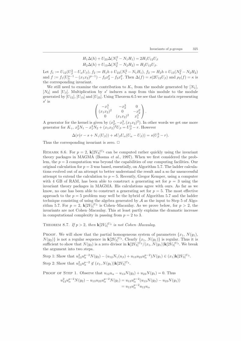
Proof. We use the description of H1(Z/3, 3V2) given in Theorem 6.5. Since we areinterested in identifying Kγ we may omit cohomology classes represented by invariants.Thus it is sufficient to consider the module generated by [N1], [N2], [Uβ ], and U12[Uβ ].Since UαU12[Uβ ] = 0, H1U12[Uβ ] = 0 and H2U12[Uβ ] = 0, we see that U12[Uβ ] is in Kγ .To describe the corresponding invariant we need to find f ∈ A2 such that ∆(f) = sU12Uβ .Let h := N1N2Uβ − U12Uβ + U23N1 −H1UαN2. Referring to the proof of Theorem 6.5,we see that

U12∆(U2β − UαUβ) = 2UαU12Uβ


H1∆(h) + U23∆(N21 −N1H1) = 2H1U12Uβ

H2∆(h) + U13∆(N22 −N2H2) = H2U12Uβ .

Let f1 := U12(U2β −UαUβ), f2 := H1h + U23(N2

1 −N1H1), f3 := H2h + U13(N22 −N2H2)

and f := f1(Up−1α − (x1x2)p−1)− f2x

p2 − f3x

p1. Then ∆(f) = s(2U12Uβ) and ρ2(f) = κ is

the corresponding invariant.We still need to examine the contribution to Kγ from the module generated by [N1],

[N2] and [Uβ ]. Multiplication by s′ induces a map from this module to the modulegenerated by [U12], [U13] and [U23]. Using Theorem 6.5 we see that the matrix representings′ is −x3

1 −x32 0

(x1x2)2 0 −xp2

0 (x1x2)2 x31

.

A generator for the kernel is given by (x32,−x3

1, (x1x2)2). In other words we get one moregenerator for Kγ , x3

2N1 − x31N2 + (x1x2)2Uβ = U3

β − r. However

∆(r(r − s + Nγ(Uβ)) + sUβUα(Uα − Uβ)) = s(U3β − r).

Thus the corresponding invariant is zero. 2

Remark 8.6. For p = 2, k[2V3]U3 can be computed rather quickly using the invarianttheory packages in MAGMA (Bosma et al., 1997). When we first considered the prob-lem, the p = 3 computation was beyond the capabilities of our computing facilities. Ouroriginal calculation for p = 3 was based, essentially, on Algorithm 5.7. The ladder calcula-tions evolved out of an attempt to better understand the result and a so far unsuccessfulattempt to extend the calculation to p = 5. Recently, Gregor Kemper, using a computerwith 4 GB of RAM, has been able to construct a generating set for p = 3 using theinvariant theory packages in MAGMA. His calculations agree with ours. As far as weknow, no one has been able to construct a generating set for p = 5. The most effectiveapproach to the p = 5 problem may well be the hybrid of Algorithm 5.7 and the laddertechnique consisting of using the algebra generated by A as the input to Step 5 of Algo-rithm 5.7. For p = 2, k[2V3]U3 is Cohen–Macaulay. As we prove below, for p > 2, theinvariants are not Cohen–Macaulay. This at least partly explains the dramatic increasein computational complexity in passing from p = 2 to 3.

Theorem 8.7. If p > 2, then k[2V3]U3 is not Cohen–Macaulay.

Proof. We will show that the partial homogeneous system of parameters {x1, N(y1),N(y2)} is not a regular sequence in k[2V3]U3 . Clearly {x1, N(y1)} is regular. Thus it issufficient to show that N(y2) is a zero divisor in k[2V3]U3/(x1, N(y1))k[2V3]U3 . We breakthe argument into two steps.

Step 1: Show that u213u

p−2α N(y2)− (u12Nγ(uβ) + u13u23u

p−2α )N(y1) ∈ (x1)k[2V3]U3 .

Step 2: Show that u213u

p−2α 6∈ (x1, N(y1))k[2V3]U3 .

Proof of Step 1. Observe that u12uα − u13N(y2) + u23N(y1) = 0. Thus

u213u

p−2α N(y2)− u13u23u

p−2α N(y1) = u13u

p−2α (u13N(y2)− u23N(y1))

= u13up−2α u12uα


and u213u

p−2α N(y2) − (u12Nγ(uβ) + u13u23u

p−2α )N(y1) = u12(u13u

p−1α − Nγ(uβ)N(y1)).

A simple calculation using the definitions of the appropriate invariants gives u13up−1α −

Nγ(uβ)N(y1) ≡ 0 (mod (x1)k[2V3]). Therefore there exists f ∈ k[2V3] such that u13

up−1α − Nγ(uβ)N(y1) = x1f . Since x1f and x1 are both elements of k[2V3]U3 we have

f ∈ k[2V3]U3 concluding the proof of Step 1.

Proof of Step 2. We use the graded reverse lexicographic order with x1 < y1 <z1 < x2 < y2 < z2. Suppose u2

13up−2α = fN(y1) + hx1 for f, h ∈ k[2V3]U3 . Since

LM(u213u

p−2α ) = xp

2yp1z2p

1 > LM(hx1) we have LM(u213u

p−2α ) = LM(fN(y1)). Therefore

LM(f) = xp2z

2p1 . We will show that there is no element of k[2V3]U3 with this lead mono-

mial. Using Theorem 8.4 we see that we need only consider elements in the algebragenerated by A. Elements from A of the form TrG

G2(Nβ(z1)e1Nβ(z2)e2ue3

β ) have degreep(e1 + e2) + 2e3 and must satisfy ei ≤ p − 1 and e1 + e2 + e3 > 2(p − 1). The smallestpossible degree for such an element is 2(p−1)+p2 and comes from taking e3 = p−1 ande1 + e2 = p. As long as p > 2, p2 +2(p− 1) > 3p and so we can restrict to the subalgebragenerated by

{xi, N(yi), N(zi) | i = 1, 2} ∪ {uα, Nγ(uβ), u12, u13, u23}.

The corresponding lead monomials are

{xi, ypi , zp2

i | i = 1, 2} ∪ {y1x2, (z1x2)p, (z1y2)p, zp1y1x2, z

p2y1x2}.

Clearly xp2z

2p1 is not a product of monomials from this list. Therefore f comes from a

tete-a-tete. All of our generators are homogeneous with respect to the bidegree so thetete-a-tete must occur in bidegree (2p, p). The monomials of bidegree (2p, p) which aregreater than xp

2z2p1 are of the form z2p

1 m where m has bidegree (0, p) and m > xp2. Since

there are no tete-a-tetes generated by monomials of this form, there is no suitable f . 2

Acknowledgements

We thank Gregor Kemper for reading an earlier draft of this paper and suggestingsome improvements and corrections. DLW’s research was partially supported by grantsfrom ARP and NSERC.

References

Almkvist, G., Fossum, R. (1978). Decompositions of Exterior and Symmetric Powers of IndecomposableZ/p-modules in Characteristic p, LNM 641, pp. 1–114. Springer.

Alperin, J. L. (1986). Local Representation Theory, Cambridge University Press.Benson, D. J. (1993). Polynomial Invariants of Finite Groups, Cambridge University Press.Bosma, W., Cannon, J. J., Playoust, C. (1997). The Magma algebra system I: the user language. J.

Symb. Comput., 24, 235–265.Campbell, H. E. A., Hughes, I. P. (1997). Vector invariants of U2(Fp): a proof of a conjecture of Richman.

Adv. Math., 126, 1–20.Cox, D., Little, J., O’Shea, D. (1992). Ideals, Varieties, and Algorithms, Springer.Dickson, L. E. (1966). On invariants and the theory of numbers. In The Madison Colloquium (1913),

Am. Math. Soc., reprinted by Dover.Eisenbud, D. (1996). Commutative Algebra with a View Toward Algebraic Geometry, Springer.Evens, L. (1991). The Cohomology of Groups, Oxford Math. Monographs, Clarendon Press.Fleischmann, P. (2000). The Noether bound in invariant theory of finite groups. Adv. Math., 152, 23–32.Fogarty, J. (2001). On Noether’s bound for polynomial invariants of a finite group. Electron. Res.

Announc. Am. Math. Soc., 7, 5–7.


Gobel, M. (1995). Computing bases for rings of permutation-invariant polynomials. J. Symb. Comput.,19, 285–291.

Gobel, M. (1998). A constructive description of SAGBI bases for polynomial invariants of permutationgroups. J. Symb. Comput., 26, 261–272.

Hughes, I., Kemper, G. (2002). Symmetric powers of modular representations, Hilbert series and degreebounds. Comm. Alg., 28, 2059–2088.

Kapur, D., Madlener, K. (1989). A completion procedure for computing a canonical basis of a k-subalgebra. In Kaltofen, E., Watt, S. eds, Proceedings of Computers and Mathematics 89, pp. 1–11.MIT.

Kemper, G. (1999). On the Cohen–Macaulay property of modular invariant rings. J. Algebra, 215,330–351.

Kemper, G. (2001). The depth of invariant rings and cohomology, (with an appendix by K. Magaard).J. Algebra, 245, 463–531.

Kemper, G. (2002). Loci in quotients by finite groups, pointwise stabilizers and the buchsbaum property.J. Reine Angew. Math., 547, 69–96.

Miller, J. L. (1996). Analogs of Grobner bases in polynomial rings over a ring. J. Symb. Comput., 21,139–153.

Noether, E. (1916). Der endlichkeitssatz der invarianten endlicher Gruppen. Math. Ann., 77, 89–92.Noether, E. (1926). Der endlichkeitssatz der invarianten endlicher linearer Gruppen der characteristik p.

Nachr. v.d.Ges. d. Wiss. zu Gottingen, 28–35.Richman, D. R. (1990). On vector invariants over finite fields. Adv. Math., 81, 30–65.Robbiano, L., Sweedler, M. (1990). Subalgebra Bases, LNM 1430, pp. 61–87. Springer.

Schwarz, G. W. (1980). Lifting smooth homotopies of orbit spaces. Inst. Hautes Etudes Sci. Publ. Math.,51, 37–135.

Shank, R. J. (1998). S.A.G.B.I. bases for rings of formal modular semiinvariants. Commentarii Mathe-matici Helvetici, 73, 548–565.

Shank, R. J., Wehlau, D. L. (1999). The transfer in modular invariant theory. J. Pure Appl. Algebra,142, 63–77.

Shank, R. J., Wehlau, D. L. (2002). Noether numbers for subrepresentations of cyclic groups of primeorder. Bull. London Math. Soc., 34, 438–450.

Smith, L. (1995). Polynomial Invariants of Finite Groups, Wellesley, MA, A. K. Peters.Sturmfels, B. (1996). Grobner Bases and Convex Polytopes, ULS 8, American Mathematical Society.Wehlau, D. L. (1993). Equidimensional representations of 2-simple groups. J. Algebra, 154, 437–489.

Computing Modular Invariants of p-groups

Documents

Transcript of Computing Modular Invariants of p-groups