arX

iv:a

lg-g

eom

/970

4009

v2 1

6 A

pr 1

997

ROZANSKY-WITTEN INVARIANTS VIA ATIYAH CLASSES

M. Kapranov

Recently, L.Rozansky and E.Witten [RW] associated to any hyper-Kahler manifold X

an invariant of topological 3-manifolds. In fact, their construction gives a system of weights

cΓ(X) associated to 3-valent graphs Γ and the corresponding invariant of a 3-manifold Y

is obtained as the sum∑cΓ(X)IΓ(Y ) where IΓ(Y ) is the standard integral of the product

of linking forms. So the new ingredient is the system of invariants cΓ(X) of hyper-Kahler

manifolds X , one for each trivalent graph Γ. They are obtained from the Riemannian

curvature of the hyper-Kahler metric.

In this paper we give a reformulation of the cΓ(X) in simple cohomological terms

which involve only the underlying holomorphic symplectic manifold. The idea is that we

can replace the curvature by the Atiyah class [At] which is the cohomological obstruction

to the existence of a global holomorphic connection. The role of what in [RW] is called

“Bianchi identities in hyper-Kahler geometry” is played here by an identity for the square

of the Atyiah class expressing the existence of the fiber bundle of second order jets.

The analogy between the curvature and the structure constants of a Lie algebra ob-

served in [RW] in fact holds even without any symplectic structure, and we study the

nonsymplectic case in considerable detail so as to make the specialization to the symplec-

tic situation easier. We show, first of all, that the Atiyah class of the tangent bundle

of any complex manifold X satisfies a version of the Jacobi identity when considered as

an element of an appropriate operad. In particular, we find (Theorem 2.3) that for any

coherent sheaf A of OX -algebras the shifted cohomology space H•−1(X, TX ⊗ A) has a

natural structure of a graded Lie algebra, given by composing the cup-product with the

Atiyah class. If E is any holomorphic vector bundle over X , then H•−1(X,E ⊗ A) is a

representation of this Lie algebra.

Then, we unravel the Jacobi identity to make the space of cochains with coefficients

in the tangent bundle into a “Lie algebra up to higher homotopies” [S]. An algebra of this

type is best described by exhibiting a complex replacing the Chevalley-Eilenberg complex

for an ordinary Lie algebra. In our case this latter complex is identified with the sheaf of

functions on the formal neighborhood of the diagonal in X ×X , the identification being

given by the “holomorphic exponential map” (the canonical coordinates of Bershadsky,

Cecotti, Ooguri and Vafa [BCOV]).

As far as the choice of cochains is concerned, we consider two versions. First, we use

Dolbeault forms (and assume that X is equipped with a Kahler metric). Second, we put

ourselves into the framework of formal geometry [B] [FGG] [GGL] and use relative forms

on the space of formal exponential maps. The underlying algebraic result here is a 1983

theorem of D.B. Fuks [Fuk] who described the stable cohomology of the Lie algebra of

1

formal vector fields with tensor coefficients in terms of what we can today identify as the

suspension of the PROP (in the sense of [Ad] ) governing weak Lie algebras. In the same

fashion, we identify (Theorem 3.7.4) a certain Gilkey-type complex of natural tensors on

Kahler manifolds with the suspended weak Lie PROP.

With the nonsymplectic case studied in detail, the introduction of a holomorphic sym-

plectic structure amounts to some easy modifications, presented in §5. As another outcome

of our considerations we obtain that the cΓ(X) can be calculated from the curvature of

an arbitrary Kahler metric, not necessarily compatible in any way with the symplectic

structure. This may be useful because the hyper-Kahler metric is rarely known explicitly.

The outline of the paper is as follows. In §1 we collect some general (well known)

properties of the Atiyah classes of arbitrary holomorphic vector bundles. In §2 we specialize

to the case of the tangent bundle, intepret the “cohomological Bianchi identity” of §1 as the

Jacobi identity and then present an unraveling of this identity on the level of Dolbeault

forms on a Kahler manifold. In §3 we recast the properties of the Atiyah class in the

language of operads and PROPs which is well suited to treat identities among operations

such as the Jacobi identity, in an abstract way. At the end of §3 we realize the weak Lie

PROP by natural differential covariants on Kahler manifolds. Section 4 is devoted to the

formal geometry analog of Kahler considerations of §§2-3. Finally, in §5 we specialize to

the case of holomorphic symplectic manifolds and show how the previous constructions

are modified and specialized in this case, in particular, how to get the Rozansky-Witten

classes cΓ(X) from the Atiyah class of X .

The author’s thinking about this question was stimulated by the letter of M. Kontse-

vich [K2] where he sketched an interpretation of Rozansky-Witten invariants by applying

the formalism of characteristic classes of (symplectic) foliations to the the ∂-foliation ex-

isting on X considered as a C∞-manifold. By trying to understand his construction, the

author arrived at the very elementary description using the Atiyah class. However, the

material of §4 comes closer to Kontsevich’s approach in that we use the formalism of tauto-

logical forms familiar in the theory of characteristic classes of foliations and Gelfand-Fuks

cohomology [B].

I would like to thank V. Ginzburg for showing me Kontsevich’s letter and V. Ginzburg

and L. Rozansky for useful discussions and suggestions which lead the paper to evolve

to its present form. Among other things, V. Ginzburg made several suggestions about

organization of the paper, in particular that I reformulate Theorem 2.6 in the form (2.8.1),

while L. Rozansky communicated to me a formula containing the germ of Theorem 2.6. I

am also grateful to M. Kontsevich who alerted me to an error in the earlier version of the

text and pointed out the reference [BCOV]. This work was partially supported by an NSF

grant and an A.P. Sloan fellowship.

2

§1. Atiyah classes in general.

(1.1) The Atiyah class of a vector bundle. Let X be a complex analytic manifold

(we can, if we want, work with smooth algebraic varieties over any field of characteristic

0). Let E be a holomorphic vector bundle on X , and J1(E) be the bundle of first jects of

sections of E. It fits into an exact sequence

(1.1.1) 0→ Ω1X ⊗E → J1(E)→ E → 0,

which therefore gives rise to the extension class

(1.1.2) αE ∈ Ext1X(E,Ω1 ⊗ E) = H1(X,Ω1 ⊗ End(E))

known as the Atiyah class of E. An equivalent way of getting αE is as follows. Let Conn(E)

be the sheaf on X whose sections over U ⊂ X are holomorphic connections in E|U . As

well known, the space of such connections is an affine space over Γ(U,Ω1 ⊗ End(E)), so

Conn(E) is a sheaf of Ω1⊗End(E))-torsors. Sheaves of torsors over any sheaf A of Abelian

groups are classified by elements of H1(X,A), and αE is the element classifying Conn(E).

So αE is an obstruction to the existence of a global holomorphic connection. If E, F are

two vector bundles, then, in obvious notation, we have:

(1.1.3) αE⊗F = αE ⊗ 1F + 1E ⊗ αF ,

because of the well known formula for the connection in a tensor product.

Let D = DX be the sheaf of rings of differential operators on X , and D≤p ⊂ D be

the subsheaf of operators of order ≤ p. It has a natural structure of OX -bimodule, the

two module structures being different. The tensor product D≤1 ⊗O E is dual to J1(E∗).

Therefore (−αE) is represented by the extension (symbol sequence)

(1.1.4) 0→ E → D≤1 ⊗O E → T ⊗ E → 0.

(1.2) The Bianchi identity. If a, b ∈ H1(X,Ω1 ⊗ End(E)) are any elements, their cup-

product a ∪ b is an element of H2(X,Ω1 ⊗ Ω1 ⊗ End(E) ⊗ End(E)). We have a natural

map of vector bundles on X

(1.2.1) Ω1 ⊗ Ω1 ⊗ End(E)⊗ End(E)→ S2(Ω1)⊗ End(E)

which is the symmetrization with respect to the first two arguments and the commutator

in the second two. We denote by [a∪ b] ∈ H2(X,S2Ω1⊗End(E)) the image of a∪ b under

the map induced by (1.2.1) in cohomology.

3

If A,B,C are three sheaves on X and u ∈ Exti(B,C), v ∈ Extj(A,B), then by

u v ∈ Exti+j(A,C) we will denote their Yoneda product.

If a is as before and c ∈ H1(X,Hom(T ⊗ T, T )) = Ext1(T ⊗ T, T ), then we denote by

a∗c ∈ H2(X,S2Ω1⊗End(E)) the Yoneda product of the embedding S2T⊗E → T⊗T⊗Eand the elements

a ∈ Ext1(T ⊗ E,E), c⊗ 1 ∈ Ext1(T ⊗ T ⊗ E, T ⊗E).

(1.2.2) Proposition. The classes αE , αT satisfy the following property (cohomological

Bianchi identity):

2[αE ∪ αE ] + αE ∗ αT = 0 in H2(X,S2Ω1 ⊗ End(E)).

Proof: Consider the two-step filtration

E ⊂ D≤1 ⊗E ⊂ D≤2 ⊗ E

with quotients E, T ⊗ E, S2T ⊗ E respectively. This filtration gives the extension classes

between consecutive quotients:

(−αE) ∈ Ext1(T ⊗ E,E), ξ ∈ Ext1(S2T ⊗E, T ⊗ E),

whose Yoneda product is 0. Our next task is to identify ξ. In fact, we have the following

lemma.

(1.2.3) Lemma. Let s : T ⊗ T → S2T be the symmetrization. Then αT⊗E ∈ Ext1(T ⊗T ⊗ E, T ⊗E) can be expressed as

αT⊗E = −ξ (s⊗ 1E)− 1T ⊗ αE .

The lemma implies (1.2.2) once we expand αT⊗E by (1.1.3).

Proof of the lemma: This is a particular case of a statement from [AL], n. (4.1.2.3)

applicable to any left D-moduleM with a good filtration (Mi) by vector bundles. In such

a situation we have the “symbol multiplication” maps

µ : T ⊗ (Mi/Mi−1)→Mi+1/Mi

induced by the D-action on M. We also have natural extension classes

fi ∈ Ext1(Mi+1/Mi,Mi/Mi−1)

(1.2.4) Lemma. [AL] In the described situation the class(−αMi/Mi−1

)is the difference

between the following two compositions (Yoneda pairings in which the degree of Ext is

indicated by square brackets):

T ⊗Mi/Mi−1µ→Mi+1/Mi

fi→Mi/Mi−1[1],

4

T ⊗Mi/Mi−11T⊗fi−1−→ T ⊗Mi−1/Mi−2[1]

µ→Mi/Mi−1[1].

To obtain Lemma 1.2.3, we take M = D ⊗ E with Mi = D≤i ⊗ E. Then for i = 1

the statement identifies (−αT⊗E). The first composition is ξ (σ ⊗ 1E), while the second

one is −1T ⊗ αE . This completes the proof.

(1.3) Atiyah class and curvature. The class αE can be easily calculated both in Cech

and Dolbeault models for cohomology. In the Cech model, we take an open covering

X =⋃Ui and pick connections ∇i in E|Ui

. Then the differences

φij = ∇i −∇j ∈ Γ(Ui ∩ Uj ,Ω1 ⊗ End(E))

form a Cech cocycle representing αE .

In the Dolbeault model, we pick a C∞-connection in E of type (1, 0), i.e., a differential

operator

∇ : E → Ω1,0 ⊗ E, ∇(f · s) = ∂(f) · s+ f · (∇s).

Let ∇ = ∇ + ∂ where ∂ is the (0,1)-connection defining the holomorphic structure. The

curvature F∇ splits into the sum F∇ = F 2,0

∇+ F 1,1

∇according to the number of antiholo-

morphic differentials. Then (see [At]).

(1.3.1) Proposition. If ∇ is any smooth connection in E of type (1,0), then F 1,1

∇is a

Dolbeault representative of αE .

(1.3.2) Remark. It may be worthwhile to explain why (1.3.1) is indeed a complete analog

of the Cech construction above. Namely, holomorphic connections in E can be identified

with holomorphic sections of a natural holomorphic fiber bundle C(E), which is an affine

bundle over Ω1 ⊗ End(E). The fiber C(E)x of C(E) at x ∈ X is the space of first jets

of fiberwise linear isomorphisms Ex × X → E defined near and identical on Ex × x.Clearly, this is an affine space over T ∗xX ⊗ End(Ex). Now, (1,0)-connections ∇ in E are

in natural bijection with arbitary C∞ sections σ of C(E). Since C(E) is a holomorphic

affine bundle, every such σ has a well defined antiholomorphic derivative ∂σ which is a

(0,1)-form with values in the corresponding vector bundle, i.e.,

∂σ ∈ Ω0,1 ⊗ Ω1,0 ⊗ End(E) = Ω1,1 ⊗ End(E).

If σ corresponds to ∇, then ∂σ = F 1,1

∇.

Proposition 1.3.1 has a corollary for Hermitian connections. Recall [W] that a Hermi-

tian metric in a holomorphic vector bundle E gives rise to a unique connection ∇ = ∇+ ∂

of the above type which preserves the metric. This connection is called the canonical con-

nection of the hermitian holomorphic bundle. It is known that F∇ is in this case of type

(1,1). Proposition 1.3.1 implies at once the following.

5

(1.3.2) Proposition. If E is equipped with a Hermitian metric and ∇ is its canonical

connection, then F∇ is a Dolbeault representative of αE .

(1.4) Atiyah class and Chern classes. If X is Kahler, then cm(E) ∈ H2m(X,C),

the mth Chern class of E, can be seen as lying in Hm(X,Ωm), and it follows that it is

recovered from the Atiyah class as follows:

(1.4.1) cm(E) = Alt(tr(αmE )).

Here αmE is an element of Hm(E, (Ω1)⊗m ⊗ End(E)) obtained using the tensor product

in the tensor algebra and the associative algebra structure in End(E), while Alt is the

antisymmetrization (Ω1)⊗m → Ωm. Note that the antisymmetrization constitutes in fact

an extra step which disregards a part of information: without it, we get an element

(1.4.2) cm(E) = tr(αmE ) ∈ Hm(X, (Ω1)⊗m).

For a vector space V let us denote by Cycm(V ) the cyclic antisymmetric tensor power of

V , i.e.,

(1.4.3) Cycm(V ) = a ∈ V ⊗m : ta = (−1)m+1a, t = (12...m),

where t is the cyclic permutation. Then, the cyclic invariance of the trace implies that

(1.4.4) cm(E) ∈ Hm(X,Cycm(Ω1)),

but it is not, in general, totally antisymmetric. We will call cm(E) the big Chern class of

E; the standard Chern class is obtained from it by total antisymmetrization.

(1.5) The Atiyah class of a principal bundle. Let G be a complex Lie group with

Lie algebra g and P → G be a principal G-bundle on X . Let ad(P ) be the vector bundle

on X associated with the adjoint representation of G. By considering connections in P ,

we obtain, similarly to the above, its Atiyah class αP ∈ H1(X,Ω1⊗ ad(P )). All the above

properties of Atiyah classes are obviously generalized to this case.

6

§2. Atiyah class of the tangent bundle and Lie brackets.

(2.1) Symmetry of the Atiyah class. Let X be as before and T = TX be the tangent

bundle of X . Specializing the considerations of (1.1) to the case when E = T , we get the

Atiyah class αTX which we can see as an element of H1(X, T ∗ ⊗ T ∗ ⊗ T ).

(2.1.1) Proposition. The element αTX is symmetric, i.e., lies in the summand

H1(X,S2(T ∗)⊗ T ).

Proof: It is enough to exhibit a sheaf of S2(T ∗) ⊗ T -torsors from which Conn(T ) (a

sheaf of T ∗ ⊗ T ∗ ⊗ T -torsors) is obtained by the change of scalars. To find it, recall that

any connection ∇ in TX has a natural invariant called its torsion τ∇ which is a section

of Λ2(T ∗) ⊗ T . The sheaf Conntf (TX) of torsion-free connections is thus a torsor over

S2(T ∗)⊗ T with required properties.

(2.2) Geometric meaning of torsion-free connections. It is convenient to “mate-

rialize” the sheaf Conntf (TX) by realizing it as the sheaf of sections of a fiber bundle

Φ(X) → X whose fiber over x ∈ X is an affine space over S2(T ∗xX) ⊗ TxX . This is

done as follows. For x ∈ X let Φx(X) be the space of second jets of holomorphic maps

φ : TxX → X with the properties φ(0) = x, d0φ = Id. A similarly defined space but

for self-maps TxX → TxX is clearly just S2(T ∗xX) ⊗ TxX . Therefore Φx(X) is an affine

space over S2(T ∗xX) ⊗ TxX . The Φx(X) for x ∈ X obviously unite into a fiber bundle

Φ(X) → X . It is well known classically that sections of this bundle are the same as

torsion-free connections.

As a corollary of this, let us note the following interpretation of αTX which can be

also deduced from Lemma 1.2.3.

(2.2.1) Proposition. The class αTX is, up to a scalar factor, represented by the following

extension (second symbol sequence):

0→ T = D≤1/D≤0 → D≤2/D≤0 → D≤2/D≤1 = S2T → 0.

We now state the first main result of this section.

(2.3) Theorem. Let X be any complex manifold and A be any quasicoherent sheaf of

commutative OX -algebras. Then:

(a) The maps

Hi(X, T ⊗ A)⊗Hj(X, T ⊗A)→ Hi+j+1(X, T ⊗ A)

given by composing the cup-product with αTX ∈ H1(X,Hom(S2T, T )), make the graded

vector space H•−1(X, T ⊗ A) into a graded Lie algebra.

(b) For any holomorphic vector bundle E on X the maps

Hi(X, T ⊗A)⊗Hj(X,E ⊗A)→ Hi+j+1(X,E ⊗ A)

7

given by composing the cup-product with the Atiyah class αE ∈ H1(X,Hom(T ⊗ E,E)),

make H•−1(X,E ⊗ A) into a graded H•−1(X, T ⊗ A)-module.

(2.3.1) Remarks. (a) By construction, the structure of a Lie algebra on the space

H•−1(X, T ⊗A) is bilinear over the graded commutative algebra H•(X,A), over which the

former space is a module. Same for the module structure on H•−1(X,E ⊗ A).

(b) To see that the graded Lie algebra structure defined above is, in general, nontrivial,

it suffices to take A = S•(T ∗) (the symmetric algebra with grading ignored), i = j = 0,

and a = b = 1 ∈ H0(X, T ⊗ T ∗). Then the bracket [a, b] ∈ H1(X, T ⊗ S2T ∗) is αTX .

(c) Theorem 2.3 is also true for sheaves of graded commutative algebras A•, if we

replace cohomology with the hypercohomology, i.e., consider

Hp(X, T ⊗ A•) =⊕

i+j=p

Hi(X, T ⊗ Aj).

(2.3) Proof of Theorem 2.3: (a) If g• is a graded vector space with an antisymmetric

bracket β :∧2

g• → g•, then the left hand side of the Jacobi identity for β is a certain

element j(β) ∈ Hom(∧3

g•, g•). In our case g• = H•−1(X, T ⊗ A) and we find that j(β)

is given by composing the cup product with a certain class

J ∈ H2(X,Hom(S3T, T )).

This class is nothing but the symmetrization of

[αTX ∪ αTX ] ∈ H2(X,S2Ω1 ⊗ Hom(T, T )),

so it vanishes by the “cohomological Bianchi identity” (1.2.2) applied to E = T .

(b) If g• is a graded Lie algebra, M• is a graded bector space with a map c : g•⊗M• →M•, then the left hand sice of the identity

[g1, g2]m− g1(g2m)− (−1)deg(g1)deg(g2)g2(g1m) = 0

is a certain element τ(c) ∈∧2

g∗⊗Hom(M,M), vanishing if and only if M is a g-module.

In our case g• = H•−1(X, T ⊗A), M• = H•−1(X,E⊗A), and the element τ(c) is induced

by a class

σ ∈ H2(X,S2Ω1 ⊗ Hom(E,E))

which is nothing but the left hand side of (1.2.2) for E. Theorem is proved.

The case A = OX does not lead to anything interesting. Indeed, we have

8

(2.3.2) Proposition. The Lie algebra structure on H•−1(X, T ) given by αTX , is trivial

(all brackets are zero). Similarly, the module structure on H•−1(X,E) is trivial.

Proof: Let a ∈ Hi(X, T ), b ∈ Hj(X, T ). By Proposition 2.2.1, the bracket [a, b] ∈Hi+j+1(X, T ) is obtained by applying to a ∪ b ∈ Hi+j(X,S2T ) the boundary homomor-

phism δ : Hi+j(X,S2T ) → Hi+j+1(X, T ) of the second symbol sequence. But we have a

pairing of sheaves

T ⊗C T → D≤1 ⊗C D≤1 → D≤2 → D≤2/D≤0,

induced by the composition of differential operators. Therefore we get an element a ⊔ b ∈Hi+j(X,D≤2/D≤0) mapping into a ∪ b. But this implies that δ(a ∪ b) = 0.

For the bundle case the argument is similar. We note that αE is represented by the

symbol sequence (1.1.4) and that we have a pairing of sheaves

T ⊗C E → D≤1 ⊗C E → D≤1 ⊗O E.

(2.4) Weak Lie algebras and their modules. Theorem 2.3 is a global cohomological

statement about the Atiyah class. We now want to give a local, cochain level strenghtening

of this result. Each time when the cohomology of some sheaf forms a graded Lie algebra, it

is natural to seek an underlying structure on the space of cochains. The standard way for

doing this is by using the concept of weak Lie algebras (or shLA’s), see [S]. Let us recall

this concept.

(2.4.1) Definition. A weak Lie algebra is a Z-graded C-vector space g• equipped with

a differential d of degree +1 and (graded) antisymmetric n-linear operations

bn : (g•)⊗n → g•, x1 ⊗ ...⊗ xn 7→ [x1, ..., xn]n, n ≥ 2, deg(bn) = 2− n,

satisfying the conditions (generalized Jacobi identities):

(2.4.2) d(bn) =∑

p+q=n

∑

σ∈Sh(p,q)

sgn(σ)bp+1(bq ⊗ 1)σ,

where Sh(p, q) is the set of (p, q)-shuffles and d(bn) is the value at bn of the natural differ-

ential in Hom((g•)⊗n, g•).

In particular, b2 is a morphism of complexes (d(b2) = 0), and it makes H•d (g•) into

a graded Lie algebra. The higher bn are the compensating terms for the violation of the

Jacobi identity on the level of cochains rather than cohomology.

An equivalent formulation of (2.4.2) is as follows [S]. Consider S(g∗[−1]), the com-

pleted symmetric algebra of the shifted dual space to g. Each bn gives a map b∗n : g∗[−1]→

9

Sn(g∗[−1]) of degree 1. Let dn be the unique odd derivation of the algebra S(g∗[−1]) ex-

tending b∗n. Then the identities (2.4.2) all together can be expressed as one condition

(2.4.3) D2 = 0, D = d+∑

n≥2

dn.

Let (g•, (bn)) be a weak Lie algebra. A weak g•-module is a graded vector space M•

equipped with a differential d of degree +1 and maps

(2.4.4) cn : (g•)⊗(n−1) ⊗M• →M•, n ≥ 2, deg(cn) = 2− n,

anntisymmetric in the first n − 1 arguments and satisfying the identities which it is

convenient to express right away in the form similar to (2.4.3). Namely, let us extend

c∗n : M• →M•⊗Sn−1(g∗[−1]) to a derivation dMn of the S(g∗[−1])-moduleM•⊗S(g∗[−1]).

Then the condition on the cn is that

(2.4.5) (1⊗D +DM )2 = 0, DM =∑

n≥2

dMn .

(2.5) Weak Lie algebra in Kahler geometry. Let X be a complex manifold. We now

unravel the Jacobi identity for the Atiyah class on the level of Dolbeault forms. Since we

will work with holomorphic as well as with antiholomorphic objects, let us agree that in the

remainder of this section T = TX will mean the holomorphic tangent bundle of X , while

Ωp,qX will signify the space of global C∞ forms of type (p, q). Similarly, for a holomorphic

vector bundle E on X we will denote by Ωp,q(E) the space of all C∞ forms of type (p, q)

with values in E.

Suppose that X is equipped with a Kahler metric h.

Let ∇ be the canonical (1, 0)-connection in T associated with h, so that (1.3):

(2.5.1) [∇,∇] = 0 in Ω2,0(End(T )).

Set ∇ = ∇ + ∂, where ∂ is the (0,1)-connection defining the complex structure. The

curvature of ∇ is just

(2.5.2) R = [∂,∇] ∈ Ω1,1(End(T )) = Ω0,1(Hom(T ⊗ T, T ))

This is a Dolbeault representative of the Atiyah class αTX , in particular,

(2.5.3) ∂R = 0 in Ω0,2(Hom(T ⊗ T, T ))

(Bianchi identity). Further, the condition for h to be Kahler is equivalent, as it is well

known, to torsion-freeness of ∇, so actually

(2.5.4) R ∈ Ω0,1(Hom(S2T, T )).

10

Let us now define tensor fields Rn, n ≥ 2, as higher covariant derivatives of the curvature:

(2.5.5) Rn ∈ Ω0,1(Hom(S2T ⊗ T⊗(n−2), T )), R2 := R, Ri+1 = ∇Ri.

(2.5.6) Proposition. Each Rn is totally symmetric, i.e., Rn ∈ Ω0,1(Hom(SnT, T )).

Proof: Follows immediately from (2.5.1).

Except for R2 = R the forms Rn are not, in general, ∂-closed. Let Ω0,•(T ) be the

Dolbeault complex of global smooth (0, i)-forms with values in T , and Ω0,•−1(T ) be the

shifted complex.

(2.6) Theorem. The maps

bn : Ω0,j1(T )⊗ ...⊗ Ω0,jn(T )→ Ω0,j1+...+jn+1(T ), n ≥ 2,

given by composing the wedge product (with values in Ω0,•(T⊗n)) with

Rn ∈ Ω0,1(Hom(T⊗n, T )), make the shifted Dolbeault complex Ω0,•−1(T ) into a weak Lie

algebra.

(2.6.1) Corollary. If X is a Hermitian symmetric space, then R makes Ω0,•−1(T ) into a

genuine Lie dg-algebra.

Proof: We need to establish the generalized Jacobi identities (2.4.1) for the Rn. For this,

write:

(2.6.2) ∂Rn = ∂∇...∇R

(with (n − 2) instances of ∇) and use the commutation relation (2.5.2) together with

(2.5.3). This gives

(2.6.3) ∂Rn =∑

a+b=n−2

∇a R∗ ∇bR,

where

R∗ ∈ Ω1,1(End(Hom(Sb+2T, T )))

is the operator-valued (1,1)-form induced by R. By evaluating R∗, we find

∂R =∑

p+q=n

∑

σ∈Sh(p,q)

Rp+1(Rq ⊗ 1)σ,

which differs from the RHS of the generalized Jacobi identity only by the absense of the

signs sgn(σ). These signs, however, constitute exactly the effect of shift from H• to H•−1.

Theorem is proved.

Remark. The first instance of Theorem 2.6 (that R3 cobounds the Jacobi identity for the

curvature) was communicated to me by L. Rozansky.

11

(2.7) Companion theorem for vector bundles. Let now (E, hE) be a Hermitian

holomorphic vector bundle on a Kahler manifold X , and let ∇E be its canonical (0,1)-

connection, so that

(2.7.1) [∇E ,∇E ] = 0 in Ω2,0(End(E)).

Let

(2.7.2) F = [∂,∇E ] ∈ Ω1,1(End(E)) = Ω0,1(Hom(T ⊗ E,E))

be the total curvature of ∇E . Then

(2.7.3) ∂F = 0 in Ω2,0(Hom(T ⊗ E,E)),

and F is the Dolbeault representative of the Atiyah class αE . Define the tensor fields

(2.7.4) Fn ∈ Ω0,1(Hom(Sn−1T ⊗ E,E))

by setting

(2.7.5) F2 = F, Fn = ∇Fn−1, n ≥ 3.

As before, the required symmetry of F follows from (2.7.1).

(2.7.6) Theorem. The maps

cn : (Ω0,•−1(T ))⊗(n−1) ⊗Ω0,•−1(E)→ Ω0,•−1(E)

given by composing the wedge product with Fn, make the Dolbeault complex Ω0,•−1(E)

into a weak module over the weak Lie algebra Ω0,•−1(T ).

The proof, using (2.7.1-3), is almost identical to that of (2.6) and is left to the reader.

(2.7.7) Corollary. If (E, hE) is a homogeneous Hermitian bundle over a Hermitian

symmetric space X , then F makes Ω0,•−1(E) into a dg-module over the dg-Lie algebra

Ω0,•−1(T ).

(2.8) Interpretation via D2 = 0. In the notation of (2.5), let

R∗n ∈ Ω0,1(Hom(T ∗, SnT ∗))

be the partial transpose of Rn. Consider the completed symmetric algebra S(T ∗) (this is

a sheaf of ungraded OX -algebras) and introduce in the algebra Ω0,•(S(T ∗)) the grading

induced from that on Ω0,•. Let R∗n be the odd derivation of this algebra induced by R∗n.

Theorem 2.6 can be reformulated as follows (I am grateful to V. Ginzburg for suggesting

that I do this).

12

(2.8.1) Reformulation. The derivation D = ∂+∑n≥2 R

∗n of Ω0,•(S(T ∗)) satisfies D2 =

0.

This is not exactly the result of applying (2.4.3) to g• = Ω0,•−1(T ) because we take

symmetric powers over OX rather than C and also do not seem to dualize the spaces Ω0,•.

But because the maps Rn areOX -linear and because the formal adjoint of ∂ : Ω0,i → Ω0,i+1

is ∂ : Ω0,r−i−1 → Ω0,r−i (r = dim(X)), this change of context is justified.

Let us now view D geometrically. The sheaf S(T ∗) is the sheaf of functions on X(∞)TX ,

the formal neighborhood of X (regarded as the zero section) in (the total space of ) TX .

More formally, denoting by π : X(∞)TX → X the natural projection, we can write

S(T ∗) = π∗(OX

(∞)

T X

).

The derivation D in Ω0,•(S(T ∗)) can thus be regarded as a non-linear (0,1)-connection D

in the fiber bundle π : X(∞)TX → X . The condition D2 = 0 means that D is integrable, i.e.,

defines a new holomorphic structure in X(∞)TX . We are going to describe this new structure

and at the same time give a very natural explanation of the previous constructions. Namely,

considerX(∞)X×X , the formal neighborhood of the diagonalX ⊂ X×X . This is a fiber bundle

over X (with respect to the projection to, say, the second factor) whose fiber over x ∈ Xis x

(∞)X = Spf(OX,x), the formal neighborhood of x in X . Clearly, this fiber bundle has a

holomorphic structure induced from that on X .

(2.8.2) Theorem. The bundle X(∞)TX with the new complex structure D is naturally

isomorphic to X(∞)X×X .

The proof is given in the next subsection.

(2.9) The holomorphic exponential map. Let x ∈ X be a point. Recall that by

TxX we denote T 1,0x X , the “holomorphic” tangent space which we want to distinguish

from TRx X , the tangent space to X conisdered as a real manifold. More precisely, let

I : TRx X → TR

x X be the complex structure, I2 = −1, and TCx X = C ⊗R TR

x X . Then

TxX is the (+i)-eigenspace of 1⊗ I on TCx X . The correspondence ξ 7→ ξ − iIξ defines an

isomorphism of complex vector spaces (TRx X, I)→ (TxX, i).

Now, the geodesic exponential map at x (for X considered as a real manifold)

expR

x : TR

x X → X

is not, in general, holomorphic. Suppose first that our Kahler metric is real analytic. Then

so is expRx , and we can take its analytic continuation “to the complex domain”. In other

words, let X ′ = X and X ′′ be X with the opposite complex structure. Then the image

of the diagonal embedding X → X ′ ×X ′′ is totally real, so X ′ ×X ′′ can be seen as the

complexification of X . Therefore expRx continues to a holomorphic map

expC

x : TC

x X = TxX ⊕ T 0,1x X → X ′ ×X ′′,

defined in some neighborhood of 0.

13

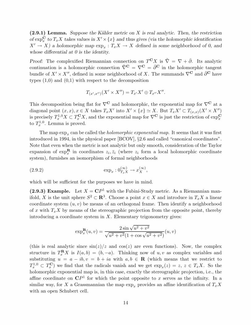
(2.9.1) Lemma. Suppose the Kahler metric on X is real analytic. Then, the restriction

of expCx to TxX takes values in X ′×x and thus gives (via the holomorphic identification

X ′ → X) a holomorphic map expx : TxX → X defined in some neighborhood of 0, and

whose differential at 0 is the identity.

Proof: The complexified Riemannian connection on TCX is ∇ = ∇ + ∂. Its analytic

continuation is a holomorphic connection ∇C = ∇C = ∂C in the holomorphic tangent

bundle of X ′×X ′′, defined in some neighborhood of X . The summands ∇C and ∂C have

types (1,0) and (0,1) with respect to the decomposition

T(x′,x′′)(X′ ×X ′′) = Tx′X ′ ⊕ Tx′′X ′′.

This decomposition being flat for ∇C and holomorphic, the exponential map for ∇C at a

diagonal point (x, x), x ∈ X takes TxX′ into X ′ × x ≃ X . But TxX

′ ⊂ T(x,x)(X′ ×X ′′)

is precisely T 1,0x X ⊂ TC

x X , and the exponential map for ∇C is just the restriction of expCx

to T 1,0x . Lemma is proved.

The map expx can be called the holomorphic exponential map. It seems that it was first

introduced in 1994, in the physical paper [BCOV], §2.6 and called “canonical coordinates”.

Note that even when the metric is not analytic but only smooth, consideration of the Taylor

expansion of expRx in coordinates zi, zi (where zi form a local holomorphic coordinate

system), furnishes an isomorphism of formal neighborhoods

(2.9.2) expx : 0(∞)TxX→ x

(∞)X ,

which will be sufficient for the purposes we have in mind.

(2.9.3) Example. Let X = CP 1 with the Fubini-Study metric. As a Riemannian man-

ifold, X is the unit sphere S2 ⊂ R3. Choose a point x ∈ X and introduce in TxX a linear

coordinate system (u, v) be means of an orthogonal frame. Then identify a neighborhood

of x with TxX by means of the stereographic projection from the opposite point, thereby

introducing a coordinate system in X . Elementary trigonometry gives:

expR

x (u, v) =2 sin

√u2 + v2

√u2 + v2(1 + cos

√u2 + v2)

(u, v)

(this is real analytic since sin(z)/z and cos(z) are even functions). Now, the complex

structure in TRx X is I(a, b) = (b,−a). Thinking now of u, v as complex variables and

substituting u = a − ib, v = b + ia with a, b ∈ R (which means that we restrict to

T 1,0x ⊂ TC

x ) we find that the radicals vanish and we get expx(z) = z, z ∈ TxX . So the

holomorphic exponential map is, in this case, exactly the stereographic projection, i.e., the

affine coordinate on CP 1 for which the point opposite to x serves as the infinity. In a

similar way, for X a Grassmannian the map expx provides an affine identification of TxX

with an open Schubert cell.

14

Let us now prove Theorem 2.8.2. Consider, for any x ∈ X , the formal isomorphism

(2.9.2). These isomorphisms unite into a fiberwise holomorphic isomorphism of fiber bun-

dles

exp : X(∞)TX → X

(∞)X×X .

The variation with respect to x of the expx is not, in general, holomorphic in the usual

sense. However, we have the following statement which implies our theorem.

(2.9.4) Proposition. The map exp is holomorphic with respect to the complex structure

D on X(∞)T .

Proof: We will consider the real analytic case. The general case presents only notational

complications in that we replace X ′ and X ′′ below by working in the variables zi and zi.

By considering the connection ∇C on X ′ ×X ′′, we reduce ourselves to the following

purely holomorphic problem.

Suppose given a complex manifold X and a family ∇ = (∇s)s∈S of flat torsion-free

connections in TX parametrized by some complex manifold S. Let p, q be the projections

of X × S to X and S respectively. Then the variation (derivative) of the ∇s with respect

to s is a section

R ∈ Γ(X × S, q∗Ω1S ⊗ p∗Hom(S2TX, TX)).

We can apply to each restriction R|X×s the covariant derivative ∇s several times, getting

tensor fields

Rn = ∇n−2R ∈ Γ(X × S, q∗Ω1S ⊗ p∗Hom(SnTX, TX)). n ≥ 2.

On the other hand, for every x, s the connection ∇s gives rise to the exponential map

expx,s : TxX → X, 0 7→ x, d0 expx,s = Id,

whose variation with respect to s is, for each fixed x, a 1-form on X with values in analytic

vector fields on (some neighborhood of 0 in) TxX with vanishing constant and linear terms.

Recall that for any vector space V the space of formal vector fields on V at 0 is the product∏n≥0 Hom(SnV, V ). Thus we can write the Taylor expansion of the variation as

exp−1x,s ds expx,s ∈ Γ

(X × S, q∗Ω1

S ⊗∏

n≥2

p∗Hom(SnTX, TX)

).

In order to establish Proposition 2.9.4, it is enough to prove the following.

(2.9.5) Proposition. In the described situation Rn is the nth homogeneous component

of exp−1x,s ds expx,s.

Proof: Fix some x0 ∈ X, s0 ∈ S and identify Tx0X with Cr, r = dim(X) by means

of some linear isomorphism. Then use expx0,s0 as a coordinate system on X near x0.

15

For any s the connection ∇s is then defined in our coordinates by its connection matrix

Γ(s) ∈ Γ(Cr,Hom(S2T, T )), so that R = dsΓ(s) is just its derivative with respect to s. For

s = s0 we have Γ(s0) = 0, because the exponential map for a flat torsion free connection

takes it into the standard Euclidean connection on the tangent space. This implies that

the higher covariant derivatives ∇is0R|X×s0 are the same as the usual derivatives, with

respect to our chosen coordinates, of Rs0 = ds|s=s0Γ(s). By the same token as before, for

arbitrary s the flatness of ∇s allows us to describe it as the connection induced from the

standard Euclidean connection on Cr by the change of coordinates given by expx0,s. So

our statement reduces to the following lemma.

(2.9.6) Lemma. Let v =∑ri=1 vi(z)∂/∂zi be a holomorphic vector field on (some domain

of) Cr. Regarding v as an infinitesimal diffeomorphism (i.e., the tangent to a family of

diffeomorphisms g(s) : Cr → Cr, s ∈ C, g(0) = Id), let Γ ∈ Γ(Cr,Hom(S2T, T )) be the

correspodning infinitesimal variation of the connmections (induced by the g(s) from the

Euclidean one). Then the components of Γ are

Γijk(z) =∂2vi∂zj∂zk

.

The proof of this lemma is straightforward from the standard formulas of differential

geometry.

16

§3. Operadic interpretation.

As we saw, for any sheaf A of commutative algebras on X , the Atiyah class αTX ∈H1(X,Hom(S2T, T )) makes each H•−1(X, T⊗A), into a graded Lie algebra. Each compos-

ite m-ary operation in this algebra (such as, e.g., [[x1, x2], [x3, x4]] for m = 4) is represented

by a certain class in Hm−1(X,Hom(T⊗m, T )) composed out of αTX . In this section we

study these classes by themselves rather than by using the operations on H•−1(X, T ⊗A))

represented by them. For this, we use the language of operads and PROPs, see [Ad] [GiK],

[GeK1-2] [KM].

(3.1) Reminder on operads, PROPs and modules. Recall that an operad P is a

collection of vector spaces P(n), n ≥ 0, together with the action of Sn, the symmetric

group, on P(n) for each n and composition maps

i : P(m)⊗ P(n)→ P(m+ n− 1), i = 1, ..., m.

satisfying appropriate equivariance and associativity axioms. Informally, elements of P(m)

can be thought as m-ary operations, the Sm-action as permutation of arguments in the

operations, and p i q as the operation

(3.1.1) p(x1, ..., xi−1, q(xi, ..., xi+n−1), xi+n, ..., xm+n−1)

An algebra over an operad P is a vector space A together with Sn-invariant maps µn :

P(n)⊗A⊗n → A satisfying the associativity properties which mean that the compositions

i in P indeed go, under the µn, into the substitution of one operation inside another, as

described in (3.1.1).

The concept of a PROP (see [Ad]) is slightly more general. While operads describe

algebras A with operations of the form A⊗n → A, PROPs allow for more general operations

A⊗n → A⊗m (which may or may not be deducible from the former ones).

Thus a PROP Π is a family of vector spaces Π(n,m), n,m ≥ 0, equipped with a

left Sn-action and a right Sm-action, commuting with each other, as well as the following

structures:

(3.1.2) Composition maps Π(n, p)⊗ Π(m,n)→ Π(m, p), making Π into a category with the

set of objects [m], m ∈ Z+ and Hom([n], [m]) = Π(n,m).

(3.1.3) Juxtaposition maps Π(n,m)⊗Π(n′, m′)→ Π(n+ n′, m+m′), making Π into a sym-

metric monoidal category with monoidal operation on objects defined by [n]⊙ [n′] =

[n+ n′].

A (right) module over an operad P is (see [M]) a collectionM of Sn-modulesM(n),

n ≥ 0 and compositions

i :M(m)⊗P(n)→M(m+ n− 1), i = 1, ..., m

17

satisfying the equivariance and associativity axioms obtained by polarizing those of an

operad.

(3.1.4) Examples. (a) For any vector space V we have its endomorphism operad EV with

components EV (n) = Hom(V ⊗n, V ) = (V ∗)⊗n⊗V . The space V is canonically an algebra

over EV . For any operad P a structure of P-algebra on a vector space A is the same as a

morphism of operads P → EA.

Similarly, we have a PROP ENDV with ENDV (n,m) = Hom(V ⊗n, V ⊗m). An algebra

over a PROP Π is a vector space A together with a morphism of PROPs Π→ ENDA. For

example, the class of Hopf algebras can be described by a PROP but not an operad.

(b) Any operad is a module over itself. If Π is a PROP, then the spaces P(n) = Π(n, 1)

form an operad. For every k the spaces Πa(n) = Π(n, a) form a module over this operad.

(3.2) dg-operads and PROPs. All the above constructions can be carried out in

any symmetric monoidal category. By a differential graded (dg-) operad we mean an

operad in the symmetric monoidal category of differential graded vector spaces, i.e., cochain

complexes (in that category the symmetry isomorphisms are given by the Koszul sign

rule). For a dg-vector space V • we define its shifts V •[m] by (V •[m])i = V m+i. For a dg-

operad P its suspension Σ(P) is a new dg-operad formed by the shifted spaces Σ(P)(n) =

P(n)[1−n] with the symmetric group action differing from that on P(n) be tensoring with

the sign representation, see [GeK1] for the explicit formulas for the compositions. If A•

is a differential graded P-algebra, then A[1] is a Σ(P)-algebra. For p ∈ P(n) let Σ(p) be

the corresponding element of Σ(P)(n). The conventions for PROPs are similar. Thus, the

suspension ΣΠ of a dg-PROP Π has ΣΠ(n,m) = Π(n,m)[m − n]. We will view graded

vector spaces as dg-vector spaces with zero differential.

(3.3) A PROP from an operad. Let P be an operad. We define a P-module P(−, 0) =

P(n, 0) called the module of natural forms (on P-algebras). It is defined as the P-module

generated by symbols

(3.3.1) tr(p) ∈ P(n, 0), p ∈ P(n+ 1),

subject to the following relations:

(3.3.2) tr(pσ) = tr(p)σ, σ ∈ Sn ⊂ Sn+1,

(3.3.3) tr(p i q) = tr(p) i q, p ∈ P(a+ 1), q ∈ P(b+ 1), i 6= a+ 1,

(3.3.4) tr(p a+1 q) = tr(q b+1 p)τ, τ =

(1 2 ... a ...a+ b

a+ 1 ... a+ b 1 ... a

),

p ∈ P(a+ 1), q ∈ P(b+ 1).

18

Motivation: if A is a finite-dimensional P-algebra, then any p ∈ P(n + 1) gives a

morphism µp : A⊗(n+1) → A, and we can take its trace trn+1(µp) : A⊗n → C with respect

to the last contravariant argument and the only covariant argument. The requirements on

the tr(p) are the axiomatizations of the properties of these traces.

We now define a PROP, denoted ΠP to be generated by formal juxtapositions and

permutations from P(n, 0) = ΠP(n, 0) and P(n) ⊂ ΠP(n, 1). In other words,

(3.3.5) ΠP(n,m) =⊕

1,...,n=A1∪...∪Am∪B1∪...∪Br

⊗

i

P(Ai)⊗⊗

j

P(Bj , 0),

where P(A),#(A) = a, is the notation for the functor on the category of a-element sets

and their bijections associated to the Sa-module P(a).

(3.3.6) Proposition. If A is a finite-dimensional P-algebra, then it is also a ΠP -algebra.

(3.4) The Lie operad and PROP. We denote by Lie the Lie operad, whose algebras

are Lie algebras in the usual sense, see [GeK1-2] [GiK]. Explicitly, Lie(n) is a subspace

in the free Lie algebra on generators x1, ..., xn spanned by Lie monomials containing each

xi exactly once. Thus Lie(2) is one-dimensional and spanned by [x1, x2] (which is anti-

invariant under S2), while Lie(3) is two-dimensional and spanned by three elements

[x1, [x2, x3]], [x2, [x1, x3]], [x3, [x1, x2]]

whose sum is zero (Jacobi identity). Given an arbitrary operad P and an element p ∈ P(2),

we will say that p is a Lie element, if p is antisymmetric and satisfies the Jacobi identity.

In other words, p is a Lie element if there is a morphism of operads Lie→ P which takes

the generator [x, y] ∈ Lie(2) into p. Such a morphism is unique, if it exists.

We denote the PROP ΠLie by LIE. The new generators in LIE (apart from the bracket

[x1, x2] ∈ LIE(2, 1)) form the space LIE(n, 0) = Lie(n, 0). An example of an element of

the latter space is given by

(3.4.1) κn = tr([x1[x2...[xn, xn+1]...]).

Here [x1[x2...[xn, xn+1]...] is regarded as an element of Lie(n+ 1). It follows from (3.3.4)

that κn is cyclically symmetric, i.e.,

(3.4.2) κnt = κn, t = (12...n) ∈ Zn ⊂ Sn.

If g is a finite-dimensional Lie algebra, then κn gives the nth Killing form on g:

(3.4.3) x1 ⊗ ...⊗ xn 7→ tr(ad(x1)...ad(xn)).

19

(3.4.4) Proposition. The space Lie(n, 0) has dimension (n − 1)! and a basis there is

formed by the elements κnσ, σ ∈ Sn/Zn.

Proof: This follows from the fact that a basis in Lie(n+1) is formed by the Lie monomials

[xσ1[...[xσ(n), xn+1]...], σ ∈ Sn.

(3.5) The Atiyah class as a Lie element. Let Now X be a complex manifold, T = TX

its tangent bundle. We have a sheaf of operads ET and a sheaf of PROPs ENDT on X

defined by

ET (n) = Hom(T⊗n, T ), ENDT (n,m) = Hom(T⊗n, T⊗m).

By applying the function H•(X,−) from sheaves to graded vector spaces, we get a graded

operad H•(X, ET ) an a graded PROP H•(X,ENDT ). Recall also (1.4) that we have the

“big Chern classes” cm(T ) ∈ Hm(X,Cycm(Ω1)) of the tangent bundle. Now, a more

inclusive formulation of the properties of the Atiyah class is by using the suspension of the

above PROP and goes as follows.

(3.5.1) Theorem. The element Σ−1αTX ∈ Σ−1H•(X, ET )(2) is a Lie element. Further-

more, the correspondence

[x1, x2] ∈ LIE(2, 1) 7→ Σ−1αTX ∈ Σ−1H•(X,ENDT )(2, 1),

κn ∈ LIE(n, 0) 7→ Σ−1cm(T ) ∈ Σ−1H•(X,ENDT )(n, 0),

defines a morphism of PROPs

LIE→ Σ−1H•(X,ENDT ) = H•(X,ENDT [−1]).

The proof follows readily from the cohomological Bianchi identity (1.2).

(3.6) Weak Lie operad and PROP. We denote by WLie the dg-operad governing

weak Lie algebras (2.4). It is generated by elements βn ∈ WLie(n), deg(βn) = 2 − n,

n ≥ 2, which are antisymmetric with respect to Sn and satisfy the conditions obtained

from Definition 2.4.1. Thus, the cohomology operad H•d (WLie) is just Lie.

The operadWLie can be also described as the cobar-construction of the commutative

operad [GiK]. Explitly, this means that a basis inWLie(n) is formed by certain trees. More

precisely, by an n-tree we mean a connected oriented graph Γ with no loops, equipped with

structures satisfying the conditions listed below.

(1) Each vertex of Γ has valency at least 3. In addition, Γ has n + 1 legs, i.e., edges

bounded by a vertex from one side only.

(2) For every vertex v all edges incident to v, except exactly one, are oriented towards v.

The set of such edges is denoted by In(v).

20

(3) It follows that all the legs of Γ expect exactly one, are oriented towards Γ. The set of

such legs is denoted by In(Γ).

(4) The set In(Γ) is identified with 1, 2, ..., n.Let T (n) be the set of isomorphism classes of n-trees. For Γ ∈ T (n) set

(3.6.1) det(Γ) =⊗

v∈Vert(Γ)

max∧(CIn(v)).

(3.6.2) Proposition. We have an identification of graded vector spaces,

WLie(n) =⊕

Γ∈T (n)

det(Γ)∗, deg(det(Γ)∗) =∑

v∈Vert(Γ)

(2− |In(v)|),

with the differential being dual to the map given by contraction of edges, and the operad

structure given by the grafting of trees, see [GiK].

Proof: The identification is obtained by associating to βn the unique n-tree with one

vertex (“corolla”) and to any composition of the βn the tree describing the composition.

The terms in the generalized Jacobi identity correspond, in geometric language, to all

possible n-trees with exactly two vertices and one edge (so that the corolla is obtained

from such a tree by contracting this unique edge).

Let WLIE be the (dg-) PROP corresponding to the dg-operad WLie as described in

(3.3). It also has a natural graphical description. Namely, call an (n,m)-graph a (not

necessarily connected) oriented raph Γ with n + m legs, of which n are inputs and are

labelled with numbers 1, ..., n, and m are outputs and are labelled by 1, ..., m, and which

satisfy the conditions (1)-(2) above. Each component of an (n,m) graph is either a tree

satisfying (1)-(3), or a graph with no output. Let G(n,m) be the set of isomorphism

classes of (n,m)-graphs. Retaining the same notations Vert, In, det, as for trees, we easily

conclude the following.

(3.6.3) Proposition. We have identifications

WLIE(n,m) =⊕

Γ∈G(n,m)

det(Γ)∗, deg(det(Γ)∗) =∑

v∈Vert(Γ)

(2− |In(v)|),

with the differential being dual to the map given by contraction of edges, composition

maps given by grafting of graphs, and juxtaposition maps given by disjoint union.

If P is any dg-operad, a family of elements pn ∈ P(n), n ≥ 2, is called a weak Lie

family, if the correspondence βn 7→ pn gives a morphism of dg-operads WLie→ P. If (pn)

is a weak Lie family, then the class of p2 in H0(P(2)) is a Lie element in H•(P). In this

case the pn give also a morphism of PROPs WLIE→ ΠP .

21

(3.7) Differential covariants and the weak Lie PROP. We now want to restate

Theorem 2.6 (which describes the unraveling of the Jacobi identity for the Atiyah class in

the framework of Kahler geometry) in a more universal form.

Notice, first of all, that the structure we really used, was not the Kahler metric itself

but only its canonical (1,0)-connection ∇. So let us call a semiflat manifold a pair (X,∇)

where X is a complex manifold and ∇ is a (1,0)-connection in TX such that [∇,∇] = 0.

For such a connection we define R = [∂,∇] and all the considerations of (2.6), (2.8) hold

true.

Fix d, i,m, n and let Cr be the sheaf of semiflat (0,1)-connections on Cr. Following

Gilkey [Gil] and Epstein [E], introduce the space V ir (n,m) of (not necessarily linear) differ-

ential operators of finite order C → Ω0,i ⊗Hom(T⊗n, T⊗m) defined in some neighborhood

of 0, and let U ir(n,m) ⊂ V ir (n,m) be the subspace of operators equivariant under the group

of holomorphic diffeomorphisms. Elements of the latter space will be called differential co-

variants of type (i, n,m) of r-dimensional semiflat manifolds, since for each such manifold

(X,∇) they produce natural tensors in Ω0,i(Hom(T⊗n, T⊗m)). In particular, they do so

for each Kahler manifold. In fact, we can say,a that elements of U ir(n,m) are differen-

tial covariants of Kahler manifolds which depend only on the canonical connection. The

differential ∂ makes U•r (n,m) into a complex; taken for all n,m, these complexes form a

dg-PROP U•r .

For example, Rn = ∇n−2R (the covariant derivative of the curvature) is an element

of U1r (n, 1). Furthermore, let Γ be a (n,m)-graph with N vertices. For every vector space

W we have the contraction map

(3.7.1) pΓ :⊗

v∈Vert(Γ)

Hom(S|In(v)|W,W )→ Hom(W⊗n,W⊗m).

Applying this to the tensor product of the R|In(v)| ∈ Ω0,1(Hom(S|In(v)|T, T )), we get a

covariant

(3.7.2) RΓ = pΓ

(⊗R|In(v)|

)∈ UNr (n,m).

Because of the symmetry of the Ri, the desuspended element Σ−1RΓ can be viewed as a

morphism

(3.7.3) Σ−1RΓ : det(Γ)∗ → Σ−1U•r (n,m).

(3.7.4) Theorem. (a) The maps Σ−1RΓ define a morphism of dg-PROPs ρ : WLIE →Σ−1U•r .

(b) For any i, n,m the morphism of vector spaces ρin,m : WLIEi(n,m) → (Σ−1Ur)i(n,m)

is surjective.

(c) If r ≫ i,m, n, then the morphism ρin,m is in fact bijective.

Part (c) means that the “stabilized” PROP of differential covariants is just the sus-

pension of the weak Lie PROP.

22

Proof: (a) Follows from Theorem 2.6.

(b) Covariants of ∇ can be viewed as covariants of the total connection ∇ = ∇ + ∂.

It is known classically that all covariants of an affine connection are obtained from the

covariant derivatives of the curvature (and torsion) by performing “tensorial contractions”.

For example, the argument sketched in [E] exhibits the Taylor expansion of the Christoffel

symbols in the normal coordinates in such a form, and this clearly suffices. In our case, the

covariant derivatives of the curvature of ∇ all reduce to the Rn, while a way to perform

the contractions produces an (n,m)-graph.

(c) This follows from the main theorem of invariant theory which implies that for

dim(W )≫ n1, ..., nN , N , the space of all GL(W )-equivariant maps

N⊗

i=1

Hom(SniW,W )→ Hom(W⊗n,W⊗m)

has as its basis, the maps pΓ for various (n,m)-graphs Γ with N vertices of valencies ni.

23

§4. The weak Lie operad in formal geometry and Gelfand-Fuks cohomology.

(4.1) The cochains. In this section we describe another way of unraveling the Jacobi

identity for the Atiyah class which uses “formal geometry” (analysis in the space of infinite

jets, see [B] [FGG] [GGL]) instead of Kahler geometry. This approach has the advantage of

being purely holomorphic. Instead of Dolbeault cochains, we will use the following lemma

to represent necessary cohomology classes.

(4.1.1) Lemma. LetX be a complex manifold and p : A→ X be a locally trivial fibration

with fibers isomorphic to CN for some N . Then for any coherent sheaf F on X we have

a natural morphism

τ : Γ(A,Ω•A/X ⊗ p∗F)→ RΓ(X,F).

If A is a Stein manifold, then τ is a quasi-isomorphism.

The first statement means that any closed relative i-form on A with values in p∗Fgives rise to a class in Hi(X,F). The second statement means that if A is Stein, then this

correspondence is 1-to-1.

Proof: Follows from the quasiisomorphism OX → p∗Ω•A/X (i.e., from the acyclicity of the

global holomorphic de Rham complex of CN ).

It was proved by Jouanolou [J] that if X is a quasi-projective algebraic manifold, then

there always exists an A as above which is an affine variety (therefore Stein). We will be

interested in some natural CN -fibrations which, though not Stein in general, still give the

holomorphic cohomology classes we need.

(4.2) Formal exponential maps. Let X be a complex manifold. Consider the space

Φ(n)(X)pn→ X of “nth order exponential maps”, cf. [B] . By definition, for x ∈ X the

fiber Φ(n)x (X) is the space of nth order jets of holomorphic maps φ : TxX → X such that

φ(0) = x, d0φ = Id. Thus Φ(2)(X) = Φ(X) is the affine fibration (2.2) defining torsion-free

connections. Thus we have a chain of projections

(4.2.1) X ← Φ(2)(X)← Φ(3)(X)← ...

Each Φ(n+1) is an affine bundle over Φ(n) whose associated vector bundle is

p∗nHom(Sn+1TX, TX). Thus each fiber of Φ(n)(X) is isomorphic to CN for some N and

Lemma 4.1.1 is applicable: every closed relative form on Φ(n)(X) gives a holomorphic

cohomology class on X .

(4.2.2) Example. Since the space Φ(X) = Φ(2)(X) is an affine bundle over

Hom(S2TX, TX), it carries a tautological 1-form α2 ∈ Ω1Φ(X)/X ⊗ p∗Hom(S2TX, TX).

This form is relatively closed and represents, via Lemma 4.1.1, the Atiyah class αTX .

Let J (n)(TX) → X be the group bundle whose fiber over x ∈ X is the group of nth

jets of biholomorphisms ψ : TxX → TxX with ψ(0) = 0, d0ψ = Id. Then Φ(n)(X) is

24

a bundle of J (n)(TX)-torsors. Let j(n)(TX) be the bundle of Lie algebras associated to

J (n)(TX). Note that we have a natural splitting

(4.2.3) j(n)(TX) =

n⊕

i=2

Hom(SiTX, TX),

induced by the action of GL(TX) on j(n)(TX).

Let now Φ := Φ(∞)(X)p→ X be the inverse limit of the diagram (4.2.1), i.e., the

space of formal exponential maps. It is a bundle of J (∞)(X)-torsors, where J (∞)(TX) =

limJ (n)(TX). The Lie algebra bundle of the bundle of proalgebraic groups J (∞)(TX) is

just

(4.2.4) j(∞)(TX) =∏

n≥2

Hom(SnT, T ), T = TX.

Denote by p(n) : Φ→ Φ(n)(X) the projection and set

(4.2.5) Ω•Φ/X =⋃

n

(p(n))∗Ω•Φ(n)(X)/X .

As with any bundle of torsors, we have the tautological relative 1-form

(4.2.6) ω ∈ Ω1Φ/X ⊗ p∗j(∞)(TX).

Projecting ω to the nth graded component in (4.2.4), we get the tautological form

(4.2.7) αn ∈ Ω1Φ/X ⊗ p∗Hom(SnT, T ).

These forms are formal geometry analogs of the covariant derivatives of the curvature in

(2.5) and satisfy very similar identities, as we shall explain later.

By the above, for every coherent sheaf F on X set

A•∞(F) = a(Φ,Ω•Φ/X ⊗ p∗F

).

This is a complex naturally mapping into RΓ(X,F). Accordingly, for any coherent sheaf of

operads P on X (i.e., an operad in the category of coherent sheaves) we have a dg-operad

A•∞(P). Similarly for PROPs.

Let us conisder, in particular, the sheaf of operads ET = Hom(T⊗n, T ) and the

sheaf of PROPs ENDT = Hom(T⊗n, T⊗m). The tautological form αn, n ≥ 2, gives an

element of A•∞ET (n) ⊂ A•∞ENDT (n, 1), which is antisymmetric and has degree 1. Consider

the desuspended dg-PROP Σ−1A•∞ENDT . The shifted tautological forms Σ−1αn becomes

antisymmetric of degree 2 − n. Further, let Γ be an (n,m)-graph (3.6) with l vertices.

We denote by αΓ ∈ Al∞ENDT (n,m) the composition of the tautological forms α|In(v)| for

all vertices v of Γ, by using the contractions along the edges of Γ. Then, because of the

antisymmetry of the Σ−1αn, we have that

Σ−1αΓ ∈ Hom(det(Γ)∗,Σ−1A•∞ENDT (n,m)).

Now, a formal geometry version of Theorem 2.6 is as follows.

25

(4.3) Theorem. The elements Σ−1αn ∈ Σ−1A•∞ET (n) form a weak Lie family. Moreover,

the maps

Σ−1αΓ : det(Γ)∗ → Σ−1A•∞ENDT (n,m), Γ ∈ G(n,m),

define a morphism of PROPs WLIE → Σ−1A•∞ENDT . In particular, the complex of

sheaves p∗Ω•−1Φ/X ⊗ T on X (quasi-isomorphic to T [−1]) has a natural structure of a weak

Lie algebra.

To formulate the companion theorem for a vector bundle E, we can proceed in a

similar way, by working on the product Φ×X C, where C is the fiber bundle over X whose

fiber at x consists of infinite jets of fiberwise linear isomorphisms Ex ×X → E identical

over x. We leave this to the reader.

We know three proofs of Theorem 4.3. The first two will be sketched, and the third

one given in more detail.

(4.3.1) First proof (sketch): We can mimic all features of Kahler geometry but on

the space Φ. First of all, the bundle Φ → X (like other infinite jet bundles, see [FGG]

[GGL]), carries a natural (non-linear) formally integrable connection D. Its covariantly

constant sections over a simply connected U ⊂ X correspond to affine structures on U , i.e.,

embeddings of U into an affine space of the same dimension, modulo affine equivalence.

This decomposes the tangent space TφΦ at every point into a direct sum T 1,0φ Φ + T 0,1

φ Φ,

where T 0,1φ is the tangent space to the fiber of p passing through φ and T 1,0

φ is the horizontal

subspace of the connection. Accordingly, we have decompositions

ΩmΦ ≃⊕

a+b=m

Ωa,bΦ , Ωa,bΦ = p∗ΩaX ⊗ ΩbΦ/X ,

and the de Rham differential is decomposed as

d = d′ + d′′, d′′ = dΦ/X , (d′)2 = (d′′)2 = [d′, d′′] = 0.

We can speak therefore about (0,1) and (1,0)-connections in fiber bundles on Φ. Every

bundle of the form p∗E, lifted from X , has a canonical integrable (0,1)-connection. The

bundle p∗T has, in addition, a natural integrable (1,0)-connection ∇ satisfying the identi-

ties

[d′′,∇] = α2, ∇αn = αn+1,

which imply our theorem in the same way as in the Kahler case.

(4.3.2) Second proof (sketch): In line with (2.8), we conisder the odd derivation D of

the algebra

Ω•Φ/X ⊗ p∗S(T ∗)

obtained by extending dΦ/X +∑n≥2 α

∗n. Then we have only to prove that D2 = 0. To do

this, we consider, as in (2.8), the fiber bundles

π : X(∞)T → X, ρ : X

(∞)X×X → X

26

where X(∞)T is the formal neighborhood of the zero section of TX and X

(∞)X×X is the formal

neighborhood of the diagonal in X ×X . The algebra S(T ∗) is just OX

(∞)T

. The pullback

to Φ of the nonlinear bundle ρ possesses an integrable connection along the fibers, which

gives rise to an algebra differential ∆ in Ω•Φ/X⊗p∗OX(∞)

X×X

satisfying ∆2 = 0. On the other

hand, on Φ we have the tautological exponential map which is a nonlinear isomorphism of

fiber bundles

Exp : p∗X(∞)T → p∗X

(∞)X×X ,

and one can verify that Exp is taking D into ∆, thereby proving the theorem.

(4.4) Tautological forms and Gelfand-Fuks cohomology. Another way of proof of

Theorem 4.3 is to reduce it to known results about the cohomology of the Lie algebra of

formal vector fields, by making use of the general relationship between this cohomology

and tautological forms. Let us first recall this relationship [B] [FGG] .

Let r ≥ 1 be fixed. Denote by G(n) the group of nth jets of biholomorphisms φ : Cr →Cr with φ(0) = 0, and by J (n) ⊂ G(n) the normal subgroup formed by φ with d0φ = Id.

So we have an exact sequence

(4.4.1) 1→ J (n) → G(n) → GLr → 1,

which, moreover, canonically splits (by considering jets of linear transformations), making

G(n) a semidirect product.

If X is an r-dimensional complex manifold and x ∈ X , let F(n)x (X) be the space of

nth jets of biholomorphisms φ : Cr → X with φ(0) = x. This is a G(n)-torsor. These

torsors unite into a principal G(n)-bundle F (n)(X)qn→ X called the bundle of nth order

frames. The quotient F (n)(X)/GLr is Φ(n)(X), the space of nth jets of exponential maps

from (4.2).

Let g = h ⊕ k be a Lie algebra split into a semidirect product of two subalgebras of

which k is an ideal. Let M be an h-module. Because of the identification g/k = h, we

can regard M as a g-module, and form the relative cochain complex

(4.4.2) C•(g,h,M) = Hom(Λ•(g/h),M)h.

Recall the following standard fact about this complex.

(4.4.3) Proposition. If g, h, k are the Lie algebras of connected Lie groups G,H,K

so that G is a semidirect product HK, then for every G-torsor P we have a natural

identification

C•(g,h,M) = Γ(P/H,Ω•P/H ⊗M)K .

Let us apply this toG = G(n), H = GLr, K = J (n). Let g(n) be the Lie algebra ofG(n).

A representation M of GLd gives rise, in a standard way, to the functor from the category

27

of r-dimensional vector spaces and their isomorphisms to the category of vector spaces

called the Schur functor and denoted by W 7→ SM (W ). In particular, the vector bundle

SM (TX) over X is defined. We denote by V the standard r-dimensional representation

of GLr. Take also P to be (fibers of) the principal G(n)-bundle F (n)(X)→ X . We obtain

the following.

(4.4.4) Proposition. We have a natural identification of complexes of sheaves on X

OX ⊗ C•(g(n), glr,M) ≃ pn∗(

Ω•Φ(n)(X)/X ⊗ q∗n(SM (TX))

)J(n)(TX)

.

Note that the tautological forms from (4.2.7) give global sections of the complex in

(4.4.4). They correspond to M = Hom(Sn(V ), V ).

By passing to the limit n→∞, we consider

(4.4.5) Vect0r = lim←

g(n) =∏

n≥1

Hom(SnV, V ),

the Lie algebra of formal vector fields on Cr vanishing at 0. This is a topological Lie

algebra and we will consider its continuous cohomology.

(4.5) The Lie operad in Gelfand-Fuks cohomology. Results of Fuks. Taking, for

every n,m ≥ 0, the relative cochain complex

(4.5.1) C•(Vect0r, glr,Hom(V ⊗n, V ⊗m)) = Π•r(n,m),

we get a dg-PROP Π•r. .Let H•r be the graded PROP formed by the cohomology of Π•r.

By the above, an element of Hir(n) gives, for each r-dimensional complex manifold X , a

class in Hi(X,Hom(T⊗n, T⊗m)). Let

an ∈ C1(Vect0r, glr,Hom(V ⊗n, V )), n ≥ 2,

be the tautological cochain which associates to a formal vector field its degree n homoge-

neous component (lying in Hom(SnV, V )). For any (n,m)-graph Γ with N vertices let

aΓ ∈ CN (Vect0r, glr,Hom(V ⊗n, V ⊗m))

be the cochain obtained by contracting the cup product of the a|In(v)|, v ∈ Vert(Γ) along

the edges of Γ, cf. (4.2). Now, Theorem 4.3 can be reformulated as follows.

(4.5.2) Theorem. Let The maps

Σ−1aΓ : det(Γ)∗ → ΠNr (n,m)

define a morphism of PROPs WLIE→ Σ−1Π•r.

In this formulation the theorem follows at once from results of D.B. Fuks [Fuk] who

studied stable cohomology of Π•r(m,n) (when r is big compared to m,n and the number

of the cohomology) and identified it with the cohomology of a certain graph complex.

Translated into our language, his results immediately imply the relation with LIE and

WLIE. More precisely, we deduce the following fact.

28

(4.5.3) Theorem. As r → ∞, each term of the complex Π•r(m,n) stabilizes, so that we

have a limit complex Π•(m,n). Taken for all m,n, these complexes form a dg-PROP,

which is isomorphic to Σ−1(WLIE).

Proof: The existence of the stabilization and its identification with a graph complex is

completely explicit in [Fuk]. Namely, the space ΠNr (n,m) consists of GLr-invariant anti-

symmetric continuous maps

(4.5.4)N∧(∏

i≥2

Hom(SiV, V )

)→ Hom(V ⊗n, V ⊗m).

Thus

(4.5.5) ΠNr (n,m) =

⊕

(Ni∈Z+)i≥2∑Ni=N

Hom

(⊗

i≥2

Ni∧Hom(SiV, V ), Hom(V ⊗n, V ⊗m)

)GLr

.

Let Γ be an (n,m)- graph (3.1) with N vertices. Then we have a natural contraction map

(4.5.6) pΓ :⊗

v∈Vert(Γ)

Hom(S|In(v)|(V ), V )→ Hom(V ⊗n, V ⊗m),

which is obviously invariant. Moreover, when r ≫ 0, then by the main theorem of invariant

theory such contraction maps for various Γ provide a basis in the space of all invariant maps.

This implies the stabilization of the Π•r(n,m). Let Ni(Γ) be the number of v ∈ Vert(Γ)

with |In(v)| = i, and let

(4.5.7) t(Γ) :⊗

i≥2

Ni(Γ)∧Hom(SiV, V )→ Hom(V ⊗n, V ⊗m)

be the antisymmetrization of pΓ. Then

t : det(Γ)∗ 7→ t(Γ)

is the desired isomorphism of complexes WLIE(n,m)→ Π•(n,m) of degreem−n. To finish

the proof, it remains to identify the composition structure in Π• with that in Σ−1(WLIE),

which is straightforward.

(4.6) Generalization to other operads. Theorem 4.5.3 can be straightforwardly gen-

eralized to any quadratic Koszul operad Q in the sense of [GiK]. Namely, let Vect0r(Q) be

the Lie algebra of derivations of FQ(r), the free Q-algebra on r generators.

29

(4.6.1) Theorem. Set

A•r,Q(m,n) = C•(Vect0r(Q), glr,Hom(V ⊗n, V ⊗m).

Then, as r → ∞, each term of A•r,Q(m,n) stabilizes, and the stable complexes A•Q(m,n)

form a dg-PROP A•Q. This PROP is isomorphic to ΠD(Q), the PROP associated (2.10) to

the dg-operad D(Q), the cobar-construction of Q. In particular, the graded PROP formed

by the cohomology of A•Q is isomorphic to Σ−1ΠQ! where Q! is the Koszul dual quadratic

operad.

This statement provides a non-symplectic analog of the result of M. Kontsevich [K1]

describing the stable cohomology of the algebra of hamiltonial vector fields. Theorem 4.5.3

corresponds to the case when Q = Com, the operad describing commutative algebras.

(4.7) Example: noncommutativization. As we could see before, all the properties of

the Atiyah class, including the detailed unraveling of the Jacobi identity, can be deduced

from the careful study of the non-linear fiber bundle on X whose fiber over x is the

formal neighborhood of x, i.e., the spectrum of the completed local algebra OX,x. This

algebra is free, i.e., isomorphic to C[[t1, ..., td]], d = dim(X), but there is no canonical

identification, the Atiyah class being an obstruction to choosing such identifications for all

x in a holomorphic way. Taken for all x ∈ X , the algebras OX,x arrange themselves into a

sheaf of complete commutativeOX -algebrasOX

(∞)

X×X

(functions on the formal neighborhood

of the diagonal), which is locally on X isomorphic to OX [[t1, ..., td]].

For any commutative ring R let R〈〈t1, ..., td〉〉 be the algebra of non-commutative

formal power series in t1, ..., td, with coefficients in R, i.e., the completion of the free

associative algebra on the xi. Now let us make the following definition.

(4.7.1) Definition. Let X be a d-dimensional complex manifold. A noncommutative

structure on X is a sheaf of complete associative OX -algebras O on X which locally on X

is isomorphic to OX〈〈t1, ..., td〉〉, together with an isomorphism O/[O,O]→ OX

(∞)X×X

.

In other words, such a structure gives, for every x ∈ X a “non-commutative for-

mal neighborhood” whose ring of functions is Ox, the fiber of O at x. These rings are

noncanonically isomorphic to C〈〈t1, ..., td〉〉(4.7.2) Example. A natural class of examples of manifolds and, more generally, stacks

with noncommutative structure is provided by the moduli spaces of vector bundles (as

opposed to more general principal G-bundles). Namely, if E is a vector bundle on an alge-

braic variety Z. Suppose that H0(X,Hom(E,E)) = C. Let M be Kuranishi deformation

space of E, so that we have a distinguished point [E] ∈ M. Then, by the general prin-

ciples of deformation theory [GM], the formal neighborhood of [E] in M is the spectrum

of H0Lie(RΓ(Z,End(E))), the zeroth Lie algebra hypercohomology of the dg-Lie algebra

RΓ(Z,End(E)). Here we regard End(E) as a sheaf of Lie algebras with respect to the

bracket [a, b] = ab− ba, thereby ignoring a richer structure of an associative algebra. If we

30

do not ignore this structure, we get an associative dg-algebra structure on RΓ(Z,End(E)).

Therefore, associative algebra hypercohomology

H0Ass(RΓ(Z,End(E)))

(to be precise, here we mean the Hochshild cohomology with C coefficients and the algebra

should be modified so as to get rid of the unity), will give us an associative algebra whose

quotient by the commutant maps naturally into the Lie algebra cohomology, i.e., into the

completed local ring ofM at [E], and under suitable conditions (when the bundle is simple

and unobstructed) this is an isomorphism.

Remark. As M. Kontsevich communicated to the author upon readind the manuscript,

he also has had the idea equivalent to Definition 4.7.1 and was aware of Example 4.7.2.

The considerations of this and the earlier sections revolve, as it is clear from con-

templating Theorem 4.5.3, around the Koszul dual pair of operads (Com,Lie): manifolds

are described by commutative algebras of functions, while the curvature data lead to Lie

algebras. So they can be generalized to manifolds with a noncommutative structure, if we

consider instead the dual pair (Ass,Ass), where Ass is the (self-dual) operad governing

associative algebras, see [GiK]. Let us summarize briefly this generalization.

(4.7.3) Theorem. Let X be a complex manifold with a noncommutative structure,

T = TX is its usual tangent bundle. Then:

(a) The second order obstruction to global trivialization of the noncommutative formal

neighborhoods is a certain class αX ∈ H1(X, T ⊗ T ) (the noncommutative Atiyah class),

whose symmetrization is the usual Atiyah class αTX .

(b) The desuspension Σ−1αX , regarded as an element of the operad Σ−1H•(X, ET ), is an

associative element, i.e., it defines a morphism of operads Ass→ Σ−1H•(X, ET ). In partic-

ular, for any sheaf A of commutative OX -algebras the shifted cohomology H•−1(X, T ⊗A)

has a natural structure of an associative algebra, given by αX .

(c) The graded Lie algebra structure on H•−1(X, T ⊗A) defined by the usual Atiyah class,

is obtained from the associative structure in (b) by the standard formula [a, b] = ab± ba.In particular, if A = OX , then the structure of an associative algebra on H•−1(X, T ) is in

fact commutative.

31

§5. The symplectic Atiyah class.

(5.1) Symmetry of the Atiyah class. Let now X be a complex manifold equipped

with a holomorphic symplectic structure. Let ω ∈ Γ(X,Ω2) be the symplectic form. We

will identify the tangent bundle T = TX with its dual T ∗ by means of ω. After this

identification, we can view the Atiyah class αTX as an element of H1(X,S2(T )⊗ T ).

(5.1.1) Proposition. The element αTX is totally symmetric, i.e., it lies in the summand

H1(X,S3(T )).

Proof: Let Symp(X) be the sheaf of connections in TX preserving the symplectic form

ω. Since for a symplectic vector space V the Lie algebra sp(V ) of infinitesimal symplectic

transformations is identified with S2(V ), the sheaf Symp(X) is, by (1.6), a torsor over

Ω1 ⊗ sp(T ) ≃ Ω1 ⊗ S2(T ) ≃ T ⊗ S2(T ). This shows that αTX is symmetric with respect

to the permutation of the second and third argument. Since it is already symmetric in the

first two arguments, the assertion follows.

(5.1.2) Remarks. One can right away exhibit an S3(T )-torsor from which αTX is ob-

tained by change of scalars. This is the torsor Symptf (X) of torsion-free symplectic con-

nections. As in (2.2), it can be materialized as the sheaf of sections of the fiber bundle

Ψ(X)→ X whose fiber Ψx(X) for x ∈ X is the space of second jets of holomorphic sym-

plectomorphisms φ : TxX → X such φ(0) = x, doφ = Id. Clearly, Ψx(X) is an affine space

over S3(TxX), and sections of Ψ are the same as torsion-free symplectic connections.

(5.2) The IHX relation for the Atiyah class. Let V be a finite-dimensional symplectic

vector space whose symplectic form is denoted by ω. Then V ∗ is also a symplectic vector

space, with respect to the inverse form ω−1. Let Γ be a finite 3-valent graph with possibly

several legs (non-compact edges bound by a vertex from one side only, cf [GeK]). Denote

by Vert(Γ),Ed(Γ),Leg(Γ) the sets of vertices, (compact) edges and legs of Γ. Let also

Flag(Γ) be the set of all flags consisting of a vertex and an incident half-edge (including

a leg) of Γ. For a vertex v let Flag(v) be the 3-element set of flags having v as a vertex.

We will distinguish between arbitrary automorphisms of Γ and strict automorphisms (i.e.,

those fixing each leg).

For a finite-dimensional vector space W we will denote by det(W ) the top exterior

power of W . If I is a finite set, then det(CI) will be abbreviated to det(I). Note that

det(I)⊗2 is canonically (i.e., Aut(I)-equivariantly) isomorphic to C. For an edge e of Γ we

denote by OR(e) the orientation line of e, i.e., OR(e) = det(∂e) where ∂e ⊂ Flag(Γ) is the

set formed by the two flags with edge e.

With these notations, note that we have a natural Sp(V )-equivariant projection

(5.2.1) pΓ : (S3(V ))⊗Vert(Γ) → (V ⊗Leg(Γ))⊗⊗

e∈Ed(Γ)

OR(e),

32

obtained by applying the form ω : V ⊗V → C to any edge of Γ. The factors OR(e) appear

because of the antisymmetry of ω.

For example, there is a unique, up to scalar, Sp(V )-equivariant antisymmetric map

(5.2.2) pIHX : S3(V )⊗ S3(V )→ S4(V ), pIHX (a⊗ b) = a, b,

the Poisson bracket of a and b considered as cubic polynomial functions on V ∗. By working

out the definition of the Poisson bracket, we find that the composition of pIHX with the

embedding S4(V ) → V ⊗4 can be represented as the sum of three projections

(5.2.3) pIHX = pI + pH + pX : S3(V )⊗ S3(V )→ V ⊗4,

where I,H,X are the three possible (up to strict isomorphism) trivalent graphs with two

vertices and the set of legs identified with 1, 2, 3, 4.

Now the Bianchi identity (1.2.2) gives, after the symmetrization, that the Atiyah class

αTX ∈ H1(X,S3(T )) satisfies the so-called IHX relation:

(5.2.4) pIHX (αTX ∪ αTX) = αTX , αTX = 0 in H2(X,S4(T )).

Of course, this can be understood from the point of view of the Lie operad, as in (3.5-6),

the graphs I,H,X corresponding to the three terms in the Jacobi identity.

(5.3) Rozansky-Witten classes. Let now Γ be a trivalent graph without legs having

l vertices. Then the projection pΓ from (5.2.1) takes values in C. By applying it to

(αTX)l ∈ H l(X, (S3(T ))⊗Vert(Γ)) we get elements

(5.3.1) cΓ(X) ∈ H l(X,O)⊗ det(Vert(Γ))⊗⊗

e

OR(e).

The factor det(Vert(Γ) appears because of the anticommutativity of the multiplication in

the cohomology, while the origin of the OR(e) was explained in (5.2). The following lemma

shows that the sign factor in (5.3.1) is the same as the one considered by Rozansky-Witten

[RW] and Kontsevich [K1].

(5.3.2) Lemma. For a trivalent graph Γ without edge-loops there is a natural (i.e.,

Aut(Γ)-equivariant) identification of 1-dimensional vector spaces

det(Vert(Γ))⊗⊗

e∈Ed(Γ)

OR(e) ≃ det(Ed(Γ))⊗ det(H1(Γ,C)) ≃

≃⊗

v∈Vert(Γ)

det(Flag(v)).

33

Proof: We start with the first isomorphism. Note that

det(Ed(Γ))⊗⊗

e∈Ed(Γ)

OR(e) ≃ det

( ⊕

e∈Ed(Γ)

OR(e)

),

while the consideration of the chain complex of Γ,

⊕

e∈Ed(Γ)

OR(e)→ CVert(Γ),

gives

det

(⊕OR(e)

)≃ det(CVert(Γ))⊗ det(H1(Γ,C)).

This implies that the tensor product of the left and the right hand sides of the first proposed

isomorphism in (3.3.2), is canonically trivial. Because det(I)⊗2 ≃ C for any finite set I,

we get the first isomorphism.

To establish the second isomorphism, consider the projections

Vert(Γ)φ←− Flag(Γ)

ψ−→ Ed(Γ).

The consideration of fibers of ψ gives

det(Flag(Γ) = det

(Ed(Γ)⊕

⊕

e

OR(e)

)= det(Ed(Γ))⊗ det(Vert(Γ))⊗ det(H1(Γ,C)),

and the consideration of fibers of φ gives that

det(Flag(Γ)) = det(Vert(Γ))⊗⊗

v∈Vert(Γ)

det(Flag(v)),

whence the statement.

For a 3-element set I a choice of direction of the real line det(RI) is the same as

a cyclic order on I. Thus the classes cΓ(X) can be seen as being elements of H l(X,O)

but defined on graphs with cyclic orders on each Flag(v) and changing the sign under the

changing of the cyclic order. Further, it follows from (5.2.3) that the cΓ thus understood

satisfy the IHX relation in the sense of [RW]. So we get the first part of the following

statement:

(5.4) Theorem. For any holomorphic symplectic manifold X the classes cΓ(X) defined

before, give rise to invariants of 3-manifolds with values in H l(X,O). If X is compact and

hyper-Kahler, then the cΓ coincide with the coefficients defined by Rozansky and Witten.

The second part just follows from the fact that the curvature represents the Atiyah

class (Proposition 1.3.1).

34

It is convenient to consider as in [RW], numerical invariants constructed from the

cΓ(X). Namely, let us put

(5.4.1) cΓ(X) = ωl/2cΓ(X) ∈ H l(X,Ωl).

Here ω ∈ H0(X,Ω2) is the symplectic form and l is the (necessarily even) number of

vertices of the 3-valent graph Γ. Further, if X is compact and L is a line bundle on X , we

define the number

(5.4.2) bΓ(X,L) =

∫

X

cΓ(X) · c1(L)dim(X)−l ∈ C.

(5.4.3) Proposition. The classes cΓ(X) and the numbers bΓ(X,L) remain unchanged if

the symplectic form ω on X is replaced by λω, λ ∈ C∗.

Proof: The class αTM ∈ H1(X,S2T ∗ ⊗ T ) does not depend on ω at all. When we write it

in the totally symmetric form, we in fact apply the isomorphism

φω : S2T ∗ ⊗ T → S2T ⊗ T

which is homogeneous in ω of degree (−2). Since every pairing corresponding to an edge

of Γ is homogeneous in ω of degree +1, we find that cΓ(X) is homogeneous of degree

−|Vert(Γ)|+ |Ed(Γ)| = −(1/2)|Vert(Γ)| = −l/2,

where we used the fact that Γ is 3-valent. Therefore cΓ(X) is homogeneous of degree 0.

(5.5) Calculation of the cΓ via non-symplectic connections. Note that the Atiyah

class αTX used to construct the cΓ, is defined in terms of the tangent bundle TX alone,

without any symplectic structure. Provided such structure ω is given, αTX just happens

to be totally symmetric in all three arguments (if we identify T ≃ T ∗ by means of ω). This

means that a Dolbeault representative of αTX in Ω0,1 ⊗ S3(TX) can be found by forcibly

symmetrizing the (1,1)-part of the curvature of any (1,0)-connection in TX . In particular,

we can take any Kahler (not necessarily hyper-Kahler) metric, write its curvature as a

section of Ω0,1 ⊗ (Ω1,0 ⊗Ω1,0 ⊗ T ), identify T with Ω1,0 via the symplectic form and then

just symmetrize with respect to the last 3 arguments. Denoting by R the corresponding

(0, 1)-form with values in S3(T ), we find:

(5.5.1) Theorem. The class cΓ is represented by the (0, l)-form pΓ(RVert(Γ)).

(5.6) Reminder on modular operads and graph complexes. We are now going

to upgrade the operadic analysis of the properties of the Atiyah class and the curvature

for general complex manifolds to the symplectic case. For this, we need the concept of a

modular operad [GeK2]. let us briefly recall this concept.

35

A stable ((g, n))-graph is a connected graph Γ with the following structures and prop-

erties:

(5.6.1) The set of legs of Γ is identified with 1, ..., n.(5.6.2) A function g : Vert(Γ)→ Z+ is given such that 2(g(v)−1)+ |v| > 0 for each vertex

v.

(5.6.3) dim(H1(Γ,C)) +∑v g(v) = g.

Let I((g, n)) be the set of isomorphism classes of stable ((g, n))-graphs, and I((g, n))

be the similar set in which we allow disconnected graphs as well.

In [GeK2], several versions of modular operads were introduced, differing by the sign

conventions (“cocycles”) entering the definition. In the present paper we are going to use

only one of them. Namely, for a stable ((g, n))-graph Γ we set

(5.6.4) ℜ(Γ) =⊗

e∈Ed(Γ)

OR(e).

The spaces ℜ(Γ) define a cocycle ℜ on the category of graphs in the sense of [GeK2], §4.

By a modular operad we will in the sequel always mean a ℜ-modular operad. Explicitly,

this is an ordinary operad P with the following additional structures:

(5.6.5) Symmetry between the inputs and the output, i.e., a Sn+1-action on P(n). To

emphasize this symmetry, we write P((n+ 1)) for P(n).

(5.6.6) A decomposition P((n)) =⊕

2g−2+n>0 P((g, n)) into Sn-invariant subspaces. The

Sn-module P((g, n) defines, in a standard way, a functor on the category of n-element sets

and bijections, whose value on a set J will be denote P((g, J)).

(5.6.7) Graphical composition maps

ℜ(Γ)⊗⊗

v∈Vert(Γ)

P((g(v),Leg(v) ))→ P((g, n)).

These structures are required to satisfy the compatibility properties given in [GeK2],

n. 4.2.

(5.7) Examples. (a) If V is a vector space with a skew-symmetric inner product B, then

we have the endomorphism modular operad E [V ] with E [V ]((g, n)) = V ⊗n for all g, the

Sn-action being the standard one and the compositions defined by contracting with help

of B. Accordingly, for a holomorphic symplectic manifold X we have a graded modular

operad H•(X, E [T ]) = H•(X, T⊗n).

(b) The suspended Lie operad ΣLie is a modular operad with ΣLie((g, n)) = 0 for

g > 0 and ΣLie(n − 1) (i.e., the space Lie(n − 1) placed in degree n − 2) for g = 0,

and with the Sn-action described in [K1], [GeK1-2]. This action arises naturally from the

36

consideration of Lie algebras with an invariant inner product. In the same way, ΣWLie is

a modular dg-operad.

(c) The graph complexes of Kontsevich [K1], once generalized to allow graphs with

legs, form a modular operad. More precisely, let G((g, n) ⊂ I((g, n)) be the set of Γ for

which all the numbers g(v) are 0. Then the condition (5.6.2) just means |v| ≥ 3 for all v,

and (5.6.3) means that the number of loops in Γ is g. Set

(5.7.1)

F((g, n)) =⊕

Γ∈G((g,n))

δ(Γ), δ(Γ) = det(Ed(Γ))∗⊗ det(H1(Γ,C))∗, deg(δ(Γ)) = |Vert(Γ).

Then the F((g, n)) form a modular dg-operad F with compositions given by grafting of

graphs and the differential dual to the one contracting edges. In fact, F is a certain twist

of FCom, the Feynman transform of the commutative operad defined in [GeK2]. We chose

the present version to avoid dealing in this paper with twists and suspensions of modular

operads and the resulting sign issues.

Note that the tree part of F is

(5.7.2) F((0, n)) = ΣWLie((n)) = ΣWLie(n− 1).

Further, F((1, n)) (the part formed by 1-loop graphs) can be expressed in terms of the

weak Lie PROP, namely it is the subcomplex in in ΣWLIE(n, 1) formed by connected

graphs. The legless part F((g, 0)) is the graph complex defined by Kontsevich in [K1].

(d) Let G((g, n)) be the subset of I((g, n)), see (5.6) formed by graphs with all g(v) = 0.

Let F((g, n)) be the space defined similarly to (5.7.1) but by summing over G((g, n)). They

form a modular dg-operad F .

(5.8) Operadic interpretation of the Jacobi identity: the level of cohomology.

Let (X,ω) be a holomorphic symplectic manifold. Then we have a graded modular operad

H•(X, E [T ]), see the example (5.7)(a). The Atiyah class αTX can be regarded as an

element of a modular operad

αTX ∈ H•(X, E [T ])((0, 3)).

(5.8.1) Theorem. The correspondence

Σ([x1, x2]) ∈ ΣLie(2) = ΣLie((0, 3)) 7→ αTX

(with Σ meaning the suspension) defines a morphism of modular operads ΣLie→ H•(X, E [T ]).

Proof: The only new property here, as compared to Theorem 3.5.1, is that we have a

morphism of modular operads, i.e., that it is invariant with respect to the action of larger

symmetric groups. But this follows from the total symmetry of αTX .

37

(5.9) Operadic interpretation: Dolbeault forms. We now look at the modular

dg-operad Ω0,•(E [T ]) = Ω0,•(T⊗n). Assume that X is equipped with a hyper-Kahler

metric h . Then the canonical (0,1)-connection ∇ of h, see (2.5), preserves the symplectic

structure. The covariant derivatives of the curvature, which we denoted Rn, n ≥ 2, are

also totally symmetric:

(5.9.1) Rn ∈ Ω0,1(Sn+1T ).

For a graph Γ ∈ G((g, n)) and a symplectic vector space W let

(5.9.2) PΓ :⊗

v∈Vert(Γ)

S|v|W → W⊗n

be the natural contraction map. Let

(5.9.3) RΓ = pΓ

( ⊗

v∈Vert(Γ)

R|v|−1

)∈ Ω0,n(T⊗n), N = |Vert(Γ)|.

Then RΓ can be regarded as a morphism

(5.9.4) RΓ : δ(Γ)→ Ω0,•(T⊗n).

(5.9.5) Theorem. The morphisms RΓ extend to a morphism of modular dg-operads

F → Ω0,•(E [T ]).

In particular, for connected graphs with no legs the tensors Ri define a morphism from

F((g, 0)) (Kontsevich’s graph complex) into the Dolbeault complex Ω0,•.

Proof: This follows from Theorem 2.6, once we take into account the additional symmetries

of the Ri.

(5.10) Operadic interpretation: formal geometry. Similarly to (4.2), let p : Ψ→ X

be the fiber bundle whose fiber at x consists of all formal symplectic exponential maps

TxX → X . This bundle carries the tautological forms

(5.10.1) αn ∈ Ω1Ψ/X ⊗ p∗Sn+1T

from which we construct the forms

(5.10.2) αΓ ∈ ΩNΨ/X ⊗ p∗T⊗n, Γ ∈ G((g, n)), |Vert(Γ)| = N,

similarly to (5.9.3).

38

(5.10.3) Theorem. The forms αΓ give rise to a morphism of modular dg-operads

F → H0(X, (p∗Ω•Ψ/X)⊗ E [T ]).

In particular, for connected graphs with no legs these form define a map of F((g, 0)) into

p∗Ω•Ψ/X .

The proof can be obtained by embedding e : Ψ → Φ where Φ is the space of all formal

exponential maps from (4.2) and noticing that αn = e∗αn, where αn is the tautological

form from (4.2.7). Our statement, which amounts to calculating dΨ/X αn, follows from

Theorem 4.3.

(5.11) Operadic interpretation: Lie algebra cohomology. The construction of

(5.10) comes close to the original approach of [K2]: even though we do not use the ∂-

foliation on X and its universal characteristic classes, the formal geometry framework can

be regarded as a holomorphic replacement of the ∂-theory. In particular, the cohomology

of the Lie algebra of formal Hamiltonian vector fields has direct interpretation in both

frameworks. The role of Fuks’ theorem (4.5.3) from the non-symplectic case is played here

by the result of Kontsevich [K1]. Let us formulate it in a more general form, allowing

graphs with legs so that the operadic formalism is applicable.

Let r be an even integer and V = Cr be the standard symplectic vector space of

dimension r. Let

(5.11.1) Ham0r =

∏

n≥2

SnV

be the Lie algebra of formal hamiltonian vector fields on V with trivial constant term. Its

degree 2 part is S2V = spr, the Lie algebra of linear symplectomorphisms. As in (4.4),

any relative cochain of (Ham0r, spr) with coefficients in some tensor power of V gives rise

to a natural relative form on Ψ/X with values in the corresponding tensor power of p∗TX .

In particular, the tautological cochain

(5.11.2) an ∈ C1(Ham0r, spr, S

n+1V )

associating to a vector field its degree n + 1 part, corresponds to the form αn. For any

graph Γ ∈ G((g, n)) define

(5.11.3) aΓ ∈ CN (Ham0r, spr, S

n+1V )

as in (5.8.9). Furthermore, the complexes

(5.11.4) P •r ((g, n)) := C•(Ham0r, spr, S

nV )

define a modular dg-operad P •r . The symplectic analog of Theorem 4.5.2 is as follows.

39

(5.11.5) Theorem. (a) The maps

aγ : δ(Γ)→ P •r ((g, n)), Γ ∈ G((g, n))

define a morphism of modular operads τ : F → P •r .

(b) If r ≫ g, n, i, then the map of vector spaces

τ : F i((g, n))→ P ir((g, n))

is an isomorphism.

This is proved in the same way as the result in [K1] (Theorem 1.1, which concerns

graphs without legs, i.e., cohomology with trivial coefficients) or [Fuk].

40

References

[Ad] J.F. Adams, Infinite Loop Spaces, Princeton Univ. Press, 1977.

[AL] B. Angeniol, M. Lejeune-Jalabert, Le theoreme de Riemann-Roch singulier pour les

D-modules, Asterisque 130 (1985), 130-160.

[At] M. F. Atiyah, Complex analytic connections in fiber bundles, Trans. AMS, 85 (1957),

181-207 (Shorter version reprinted in his Collected Papers, vol.1, p. 95-102, Clarendon

Press, Oxford, 1988).

[BCOV] M. Bershadsky, S. Cecotti, H. Ooguri, C. Vafa, Kodaira-Spencer theory of gravity

and exact results for quantum string amplitudes, Comm. Math. Phys. 165 (1994), 311-

428.

[B] R. Bott, Some aspects of invariant theory in differential geometry, in: “Differential

operators on Manifolds” (CIME), p. 49-145, Edizione Cremonese, 1975 (Reprinted in his

Collected Papers, vol. 3, p. 357-453, Birkhauser, Boston, 1996).

[E] D.B.A. Epstein, Natural tensors on Riemannian manifolds, J. Diff. geom. 10 (1975),

631-645.

[Fuk] D.B. Fuks, Stable cohomologies of a Lie algebra of formal vector fields with tensor

coefficients, Funct. Anal. Appl. 17 (1983), 295-301.

[FGG] D.B. Fuchs, I.M. Gelfand, A.M. Gabrielov, The Gauss-Bonnet theorem and the

Atiyah-Patodi-Singer functionals for the characteristic classes of foliations, Topology, 15

(1976), 165-188. (Reprinted in: Collected Papers of I.M. Gelfand, Vol. 3, p. 379-402,

Springer-Verlag, 1989)

[GGL] A.M. Gabrielov, I.M. Gelfand, M.V. Losik, Combinatorial computation of charac-

teristic classes, Funct. Anal. Appl. 9 (1975), 103-115. (Reprinted in: Collected Papers of

I.M. Gelfand, Vol. 3, p. 407-419, Springer-Verlag, 1989)

[GeK1] E. Getzler, M. Kapranov, Cyclic operads and cyclic homology, in: “Geometry,

Topology and Physics for R. Bott” (S.-T. Yau, Ed.) p. 167-201, International Press,

Boston, 1995.

[GeK2] E. Getzler, M. Kapranov, Modular operads, preprint dg-ga/9408003, to appear in

Compositio Math.

[Gil] P.B. Gilkey, Curvature and eigenvalues of the Dolbeault complex for Kahler manifolds,

Adv. in Math. 11 (1973), 311-325.

[GiK] V. Ginzburg, M. Kapranov, Koszul duality for operads, Duke Math. Journal, 76

(1994), 203-272.

41

[GM] W.M. Goldman, J.J. Millson, The deformation theory of representations of funda-

mental groups of compact Kahler manifolds, Publ. IHES, 67 (1988), 43-96.

[J] J.-L. Jouanolou, Une suite exacte de Mayer-Vietoris dans la K-theorie algebrique, in:

Lecture Notes in Math., 341, p. 293-316, Springer-verlag, 1973.

[K1] M. Kontsevich, Formal noncommutative symplectic geometry, in “Gelfand Mathemat-

ical Seminars 1990-92” (L. Corwin, I. Gelfand, J. Lepowski Eds.) p. 173-187, Birkhauser,

Boston, 1993.

[K2] M. Kontsevich, letter to V. Ginzburg, Jan. 8, 1997.

[KM] I. Kriz, J.P. May, Operads, Algebras, Modules and Motives, Asterisque 233, Soc.

Math. France, 1995.

[M] M. Markl, Models for operads, Comm. in Algebra, 24 (1996), 1471-1500.

[RW] L. Rozansky, E. Witten, Hyper-Kahler geometry and invariants of 3-manifolds,

preprint hep-th/9612216.

[S] J. Stasheff, Differential graded Lie algebras, quasi-Hopf algebras and higher homotopy

algebras, in: Lecture Notes in Math., 1510, p. 120-137, Springer-Verlag, 1992.

[W] R.O. Wells, Differential calculus on complex manifolds, Springer-Verlag, 1982.

Department of Mathematics, Northwestern University, Evanston IL 60208,

email: kapranov@math.nwu.edu

42