Multiplicities of Schur functions in invariants of two 3×3 matrices
24
Journal of Algebra 264 (2003) 496–519 www.elsevier.com/locate/jalgebra Multiplicities of Schur functions in invariants of two 3 × 3 matrices ✩ Vesselin Drensky ∗ and Georgi K. Genov Institute of Mathematics and Informatics, Bulgarian Academy of Sciences, Acad. G. Bonchev Str., Block 8, 1113 Sofia, Bulgaria Received 13 March 2002 Communicated by Susan Montgomery Abstract We relate with any symmetric function f(x,y) ∈ C❏x,y❑ presented as an infinite linear com- bination of Schur functions f(x,y) = ∑ m(λ 1 ,λ 2 )S (λ 1 ,λ 2 ) (x,y) the multiplicity series M(f) = ∑ m(λ 1 ,λ 2 )t λ 1 u λ 2 . We study the behavior of M(f) under natural combinatorial and algebraic con- structions. In particular, we calculate the multiplicity series for the symmetric algebra of the irre- ducible GL 2 (C)-module corresponding to the complete symmetric function of degree 3. Our main result is that we have found the explicit form of the multiplicity series for the Hilbert (or Poincaré) series of the algebra of invariants of two 3 × 3 matrices. As a consequence, we have precised the re- sult of Berele on the asymptotics of the multiplicities in the trace cocharacter sequence of two 3 × 3 matrices. 2003 Elsevier Science (USA). All rights reserved. MSC: 16R30; 05E05 Keywords: Matrix invariants; Trace rings; Symmetric functions; Schur functions 1. Introduction Let C❏x,y ❑ be the algebra of formal power series in two variables equipped with its usual (formal power series) topology and let ✩ Partially supported by Grant MM-1106/2001 of the Bulgarian Foundation for Scientific Research. * Corresponding author. E-mail addresses: [email protected] (V. Drensky), [email protected] (G.K. Genov). 0021-8693/03/$ – see front matter 2003 Elsevier Science (USA). All rights reserved. doi:10.1016/S0021-8693(03)00070-X
-
Upload
independent -
Category
Documents
-
view
3 -
download
0
Transcript of Multiplicities of Schur functions in invariants of two 3×3 matrices

a
-
n-irre-
mainaré)e re-3
h its
Journal of Algebra 264 (2003) 496–519
www.elsevier.com/locate/jalgebr
Multiplicities of Schur functions in invariantsof two 3× 3 matrices
Vesselin Drensky∗ and Georgi K. Genov
Institute of Mathematics and Informatics, Bulgarian Academy of Sciences, Acad. G. Bonchev Str., Block 8,1113 Sofia, Bulgaria
Received 13 March 2002
Communicated by Susan Montgomery
Abstract
We relate with any symmetric functionf (x, y) ∈ Cx, y presented as an infinite linear combination of Schur functionsf (x, y) = ∑
m(λ1, λ2)S(λ1,λ2)(x, y) the multiplicity seriesM(f ) =∑m(λ1, λ2)t
λ1uλ2. We study the behavior ofM(f ) under natural combinatorial and algebraic costructions. In particular, we calculate the multiplicity series for the symmetric algebra of theducibleGL2(C)-module corresponding to the complete symmetric function of degree 3. Ourresult is that we have found the explicit form of the multiplicity series for the Hilbert (or Poincseries of the algebra of invariants of two 3× 3 matrices. As a consequence, we have precised thsult of Berele on the asymptotics of the multiplicities in the trace cocharacter sequence of two× 3matrices. 2003 Elsevier Science (USA). All rights reserved.
MSC: 16R30; 05E05
Keywords: Matrix invariants; Trace rings; Symmetric functions; Schur functions
1. Introduction
Let Cx, y be the algebra of formal power series in two variables equipped witusual (formal power series) topology and let
Partially supported by Grant MM-1106/2001 of the Bulgarian Foundation for Scientific Research.* Corresponding author.
E-mail addresses: [email protected] (V. Drensky), [email protected] (G.K. Genov).
0021-8693/03/$ – see front matter 2003 Elsevier Science (USA). All rights reserved.doi:10.1016/S0021-8693(03)00070-X

V. Drensky, G.K. Genov / Journal of Algebra 264 (2003) 496–519 497
tions
f thee
w
for
Symx, y = Cx, yS2
be the subalgebra of symmetric functions. It is well known that the set of Schur funcSλ(x, y)= S(λ1,λ2)(x, y) | λ= (λ1, λ2) ∈ Z × Z, λ1 λ2 0
forms a basis of the topological vector space Symx, y. Any symmetric function in twovariables has the presentation
f (x, y)=∑i,j0
a(i, j)xiyj =∑
λ=(λ1,λ2)
m(λ)Sλ(x, y), (1)
wherea(i, j) = a(j, i) ∈ C for all i, j 0 andm(λ) ∈ C is the multiplicity of Sλ(x, y)in the decomposition off (x, y). In the special case, whenf (x, y) = Hilb(W,x, y) isthe Hilbert (or Poincaré) series of a direct sumW of irreducible polynomialGL2(C)-modulesW(λ), the nonnegative integerm(λ) is equal to the multiplicity ofW(λ) in thedecomposition ofW as a direct sumW =∑⊕
λ m(λ)W(λ). The coefficientsa(i, j) and themultiplicitiesm(λ) of f (x, y) in (1) are related by
m(λ1, λ2)= a(λ1, λ2)− a(λ1 + 1, λ2 − 1), (2)
wherea(λ1 + 1, λ2 − 1)= 0 if λ2 = 0, see, e.g., [1].For many applications, it is important to know the explicit form or the asymptotics o
multiplicitiesm(λ) of a given symmetric functionf (x, y). For this purpose, we introducthe multiplicity series
M(f )(t, u)=∑
λ1λ20
m(λ1, λ2)tλ1uλ2 ∈ Ct, u (3)
of the symmetric functionf (x, y) ∈ Symx, y in (1).The mappingM : Symx, y → Ct, u is continuous and linear. If we introduce a ne
variablev = tu, thenM is a bijection of Symx, y onto the subalgebra ofCt, u
Ct, v = ∑λ1λ20
m(λ1, λ2)tλ1−λ2(tu)λ2
∣∣∣m(λ1, λ2) ∈ C
.
We shall denoteM(f ) also as
M ′(f )(t, v)=M(f )(t, u)=∑
λ1λ20
m(λ1, λ2)tλ1−λ2vλ2 ∈ Ct, v. (4)
The main purpose of our paper is to find the explicit form of the multiplicity seriesthe Hilbert series
Hilb(C2,3, x, y)=∑
dimC C(m,n)2,3 xmyn
m,n0

498 V. Drensky, G.K. Genov / Journal of Algebra 264 (2003) 496–519
nt
ofof
ities,.g. the
ebra
f thereisrs of
tainednts of.)
es of, we
of the centerC2,3 of the algebra with trace generated by two generic 3× 3 matricesξ = (ξij ) and η = (ηij ), where ξij , ηij , i, j = 1,2,3, are algebraically independe
commuting variables, and the vector spaceC(m,n)2,3 is the homogeneous component
bidegree(m,n) with respect toξ andη. The algebraC2,3 coincides with the subalgebraGL3(C)-invariants inΩ = C[ξij , ηij | i, j = 1,2,3] under the action ofGL3(C) inducedby the simultaneous conjugation onξ andη.
The centerCp,k of the algebra with trace generated byp generick×k matrices is amongthe important objects in invariant theory, theory of algebras with polynomial identtheory of division algebras, representation theory of symmetric groups, etc., see ebook by Formanek [5]. Its numerical parameters are objects of intensive study.
The explicit form of the Hilbert series ofC2,3 was obtained by Teranishi [9]:
Hilb(C2,3, x, y) = (1+ x3y3) 1
1− x2y2
1
(1− x)(1− y)
1
(1− x2)(1− xy)(1− y2)
× 1
(1− x3)(1− x2y)(1− xy2)(1− y3). (5)
Berele [1] found the asymptotics of its multiplicitiesm(λ1, λ2).The series Hilb(C2,3, x, y) is a product of the Hilbert series of several naturalGL2(C)-
modules:
C ⊕W(3,3), C[W(2,2)
], C
[W(1,0)
], C
[W(2,0)
], C
[W(3,0)
],
whereC[W(λ)] is the symmetric algebra of the irreducibleGL2(C)-moduleW(λ). ThealgebraC[W(λ1, λ2)] is isomorphic as a bigraded algebra to the polynomial algC[zij | i, j λ2, i + j = λ1 + λ2], where the variablezij is of bidegree(i, j). Hence,as aGL2(C)-module,C2,3 may be considered as the tensor product
C2,3 ∼= (C ⊕W(3,3)
)⊗ C[W(2,2)
]⊗ C[W(1,0)
]⊗ C[W(2,0)
]⊗ C[W(3,0)
].
It has turned out that the multiplicity series behave very well under multiplication osymmetric function with the Hilbert series ofW(λ1, λ2), and of its symmetric algebra foλ1 = λ2, and forλ = (1,0) andλ = (2,0). Hence, the main difficulty is to evaluate thmultiplicity series for Hilb(C[W(3,0)], x, y). We have obtained its explicit form and thresult is in the spirit of a classical result of Thrall [10] on symmetrized tensor poweW(2,0) (but the result of Thrall is for theGLk(C)-moduleWk(2,0, . . . ,0) for anyk 2).
As a consequence of our main result we have corrected the asymptotic result obby Berele [1]. (Due to a technical error (an omitted summand) some of the coefficiethe polynomials in the asymptotics of Berele are slightly different from the real ones
Some of the calculations we performed or checked using MAPLE. We have foundvarious expressions for the multiplicities of the Schur functions in the Hilbert seriC[W(3,0)] andC2,3 but we have not included them in the present text. In particularhave explicit (and quite complicated) formulas for the multiplicities forC2,3. We mayprovide detailed data by request (e.g., we may send by e-mail a file in a MAPLE-format).
The main results of the present paper have been announced in [3].

V. Drensky, G.K. Genov / Journal of Algebra 264 (2003) 496–519 499
ouretric
Since, manyal casebe
tably
the
2. Preliminaries
Although our results hold over any field of characteristic 0, we shall restrictconsiderations overC. We summarize the necessary background on theory of symmfunctions in two variables. Details can be found, e.g., in the book by Macdonald [6].the symmetric functions in two variables are much simpler than in the general caseof the results can be obtained directly, without using the general theory. In the speciof two variables, the Schur functionSλ(x, y) has the following expression which mayconsidered as a definition:
Sλ(x, y) = (xy)λ2(xa + xa−1y + xa−2y2 + · · · + xya−1 + ya
)= (xy)λ2(xλ1−λ2+1 − yλ1−λ2+1)
x − y,
where we have denoteda = λ1 − λ2. In particular,
S(c,c)(x, y)= (xy)c, S(a+b+c,b+c)(x, y)= S(c,c)(x, y)S(a+b,b)(x, y), (6)
1
1− (xy)b=∑n0
(xy)bn =∑n0
S(bn,bn)(x, y).
It is well known (and can be easily obtained directly) that
1
(1− x)(1− y)=∑n0
S(n,0)(x, y), (7)
1
(1− x2)(1− xy)(1− y2)=
∑λ=(λ1,λ2)
S(2λ1,2λ2)(x, y). (8)
The equality (8) is a partial case of the general fact for symmetric functions in counmany variables
∏ij
1
1− xixj=∑λ
S2λ(x1, x2, . . .),
where 2λ = (2λ1,2λ2, . . .). This expresses also the result of Thrall [10] aboutdecomposition of the symmetric algebra of the irreducibleGLk(C)-moduleWk(2)
C[Wk(2)
]= C[Wk(2,0, . . . ,0︸ ︷︷ ︸)]∼=
∑λ
Wk(2λ).
k−1 times

500 V. Drensky, G.K. Genov / Journal of Algebra 264 (2003) 496–519
r
ies
We shall also need the Young rule for the product of Schur functions of the formSλS(c,0).In the case of two variables it has the following simple form:
S(a+b,b)(x, y)S(c,0)(x, y)=min(a,c)∑d=0
S(a+b+c−d,b+d)(x, y). (9)
In other words,Sλ(x, y)S(c,0)(x, y) = ∑Sµ(x, y) is a sum of pairwise different Schu
functionsSµ(x, y). The Young diagrams[µ] = [µ1,µ2] corresponding to the partitionsµindexing the summandsSµ(x, y) are obtained from the diagram[λ] by addingc boxes insuch a way that no two new boxes are in the same column of[µ]. (Whenc = 1 this is thewell-known Branching theorem.) For example, ifλ= (3,1) andc = 3, we obtain
S(3,1)(x, y)S(3,0)(x, y)= S(6,1)(x, y)+ S(5,2)(x, y)+ S(4,3)(x, y),
and present it graphically as
× X X X = X X X + X XX + X
X X .
In the sequel we fix the notationv = tu and for a symmetric functionf (x, y) ∈Symx, y in the form (1) we define the multiplicity seriesM(f )(t, u) = M ′(f )(t, v) inthe forms (3) and (4).
Lemma 1.(i) For any symmetric function f (x, y) ∈ Symx, y and any formal power series g(z)
depending on z= xy only,
M(g(xy)f (x, y)
)= g(tu)M(f )(t, u)= g(v)M ′(f )(t, v). (10)
(ii) The symmetric function f (x, y) and its multiplicity series M(f )(t, u) = M ′(f )(t, v)are related by
f (x, y)= xM(f )(x, y)− yM(f )(y, x)
x − y= xM ′(f )(x, xy)− yM ′(f )(y, xy)
x − y. (11)
Proof. (i) Since the operatorM is continuous with respect to the formal power sertopology, it is sufficient to prove (10) only forf (x, y)= S(λ1,λ2)(x, y) andg(xy)= (xy)c
when (10) follows immediately from (6):
M((xy)cS(λ1,λ2)(x, y)
) = M(S(λ1+c,λ2+c)(x, y)
)= tλ1+cuλ2+c
= (tu)c(tλ1uλ2
)= (tu)cM(S(λ1,λ2)(x, y)
).
V. Drensky, G.K. Genov / Journal of Algebra 264 (2003) 496–519 501
ted
v [8]outatorics
ator
n be
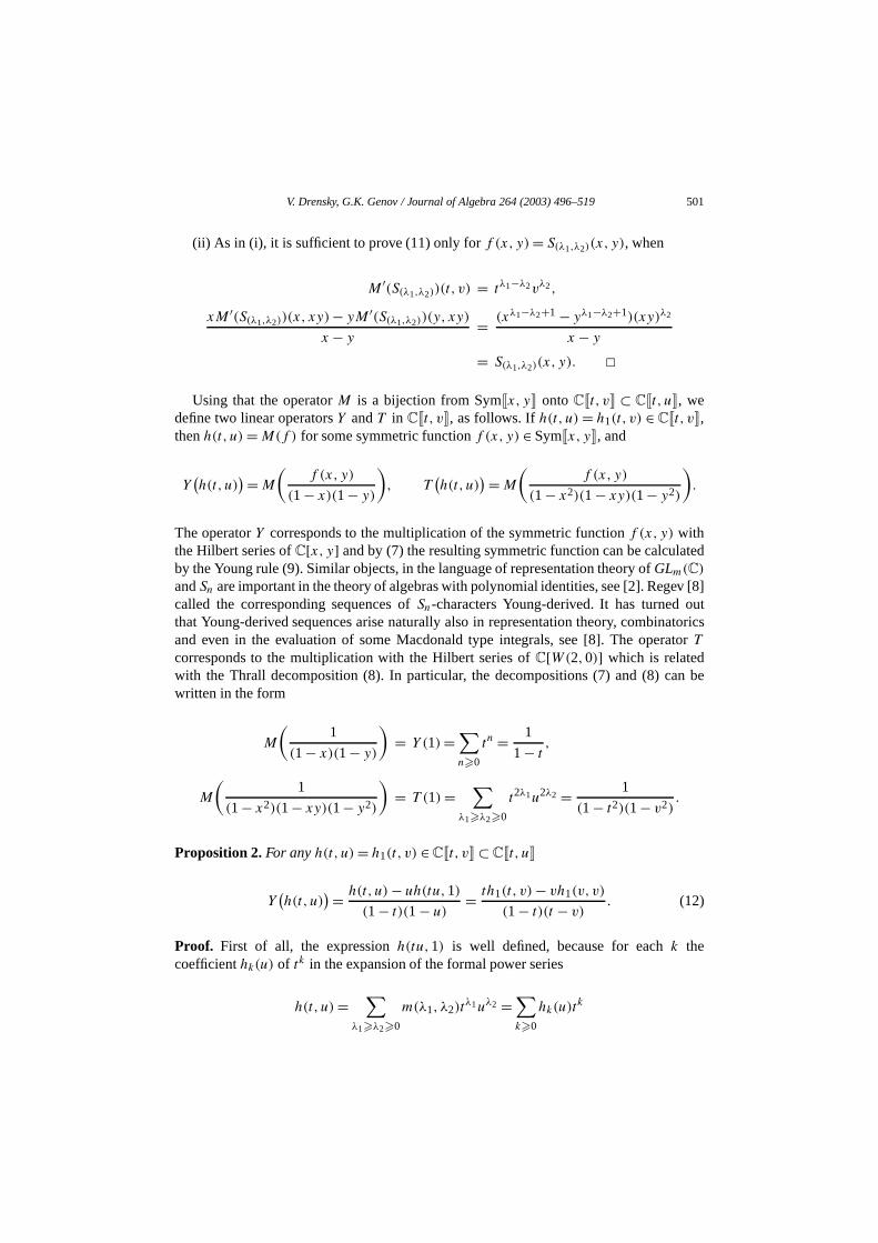
(ii) As in (i), it is sufficient to prove (11) only forf (x, y)= S(λ1,λ2)(x, y), when
M ′(S(λ1,λ2))(t, v) = tλ1−λ2vλ2,
xM ′(S(λ1,λ2))(x, xy)− yM ′(S(λ1,λ2))(y, xy)
x − y= (xλ1−λ2+1 − yλ1−λ2+1)(xy)λ2
x − y
= S(λ1,λ2)(x, y). Using that the operatorM is a bijection from Symx, y onto Ct, v ⊂ Ct, u, we
define two linear operatorsY andT in Ct, v, as follows. Ifh(t, u)= h1(t, v) ∈ Ct, v,thenh(t, u)=M(f ) for some symmetric functionf (x, y) ∈ Symx, y, and
Y(h(t, u)
)=M
(f (x, y)
(1− x)(1− y)
), T
(h(t, u)
)=M
(f (x, y)
(1− x2)(1− xy)(1− y2)
).
The operatorY corresponds to the multiplication of the symmetric functionf (x, y) withthe Hilbert series ofC[x, y] and by (7) the resulting symmetric function can be calculaby the Young rule (9). Similar objects, in the language of representation theory ofGLm(C)andSn are important in the theory of algebras with polynomial identities, see [2]. Regecalled the corresponding sequences ofSn-characters Young-derived. It has turnedthat Young-derived sequences arise naturally also in representation theory, combinand even in the evaluation of some Macdonald type integrals, see [8]. The operTcorresponds to the multiplication with the Hilbert series ofC[W(2,0)] which is relatedwith the Thrall decomposition (8). In particular, the decompositions (7) and (8) cawritten in the form
M
(1
(1− x)(1− y)
)= Y (1)=
∑n0
tn = 1
1− t,
M
(1
(1− x2)(1− xy)(1− y2)
)= T (1)=
∑λ1λ20
t2λ1u2λ2 = 1
(1− t2)(1− v2).
Proposition 2. For any h(t, u)= h1(t, v) ∈ Ct, v ⊂ Ct, u
Y(h(t, u)
)= h(t, u)− uh(tu,1)
(1− t)(1 − u)= th1(t, v)− vh1(v, v)
(1− t)(t − v). (12)
Proof. First of all, the expressionh(tu,1) is well defined, because for eachk thecoefficienthk(u) of tk in the expansion of the formal power series
h(t, u)=∑
m(λ1, λ2)tλ1uλ2 =
∑hk(u)t
k
λ1λ20 k0
502 V. Drensky, G.K. Genov / Journal of Algebra 264 (2003) 496–519
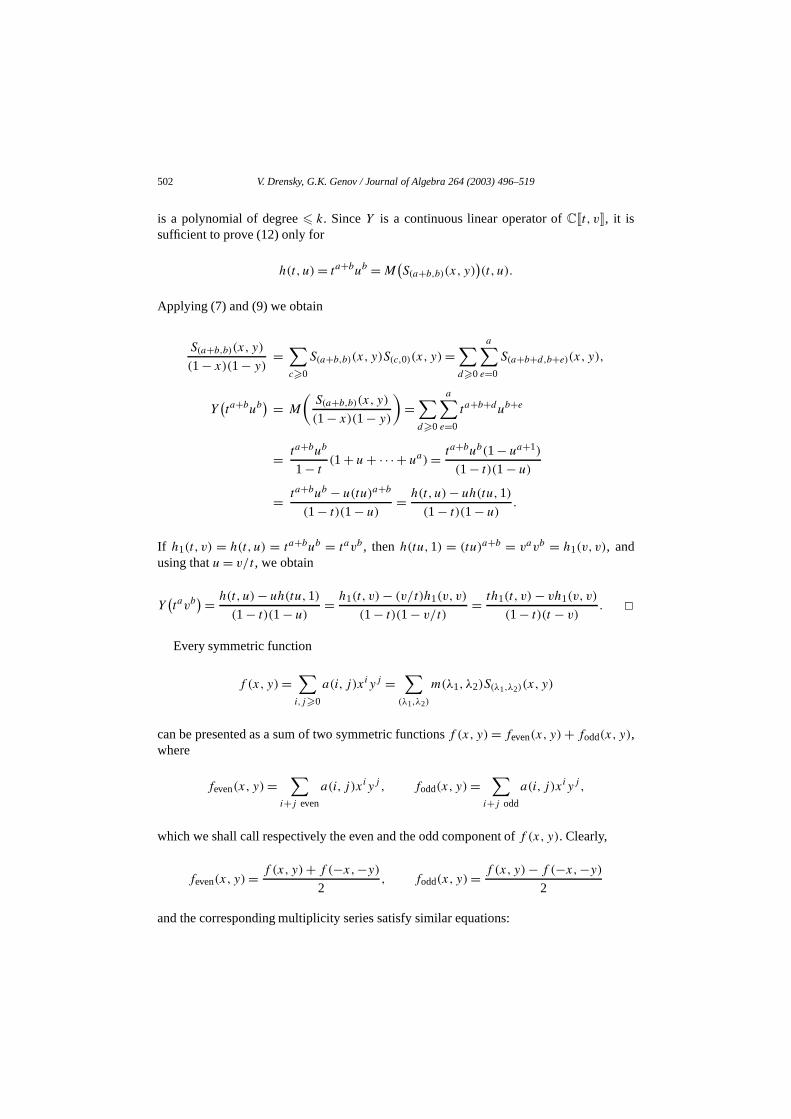
is a polynomial of degree k. SinceY is a continuous linear operator ofCt, v, it issufficient to prove (12) only for
h(t, u)= ta+bub =M(S(a+b,b)(x, y)
)(t, u).
Applying (7) and (9) we obtain
S(a+b,b)(x, y)(1− x)(1− y)
=∑c0
S(a+b,b)(x, y)S(c,0)(x, y)=∑d0
a∑e=0
S(a+b+d,b+e)(x, y),
Y(ta+bub
) = M
(S(a+b,b)(x, y)(1− x)(1− y)
)=∑d0
a∑e=0
ta+b+dub+e
= ta+bub
1− t(1+ u+ · · · + ua)= ta+bub(1− ua+1)
(1− t)(1 − u)
= ta+bub − u(tu)a+b
(1− t)(1− u)= h(t, u)− uh(tu,1)
(1− t)(1− u).
If h1(t, v) = h(t, u) = ta+bub = tavb , thenh(tu,1) = (tu)a+b = vavb = h1(v, v), andusing thatu= v/t , we obtain
Y(tavb
)= h(t, u)− uh(tu,1)
(1− t)(1− u)= h1(t, v)− (v/t)h1(v, v)
(1− t)(1− v/t)= th1(t, v)− vh1(v, v)
(1− t)(t − v).
Every symmetric function
f (x, y)=∑i,j0
a(i, j)xiyj =∑
(λ1,λ2)
m(λ1, λ2)S(λ1,λ2)(x, y)
can be presented as a sum of two symmetric functionsf (x, y)= feven(x, y)+ fodd(x, y),where
feven(x, y)=∑
i+j even
a(i, j)xiyj , fodd(x, y)=∑
i+j odd
a(i, j)xiyj ,
which we shall call respectively the even and the odd component off (x, y). Clearly,
feven(x, y)= f (x, y)+ f (−x,−y)
2, fodd(x, y)= f (x, y)− f (−x,−y)
2
and the corresponding multiplicity series satisfy similar equations:

V. Drensky, G.K. Genov / Journal of Algebra 264 (2003) 496–519 503
M(feven)(t, u) =∑
λ1+λ2 even
m(λ1, λ2)tλ1uλ2,
M(fodd)(t, u) =∑
λ1+λ2 odd
m(λ1, λ2)tλ1uλ2,
M(feven)(t, u) = M(f )(t, u)+M(f )(−t,−u)
2,
M(fodd)(t, u) = M(f )(t, u)−M(f )(−t,−u)
2.
We shall also callM(feven) andM(fodd) respectively even and odd multiplicity series.
Proposition 3.(i) For any even multiplicity series h(t, u) ∈ Ct, v ⊂ Ct, u
T(h(t, u)
)= 1
(1− t2)(1− u2)
(h(t, u)
1− tu− u(t + u)h(tu,1)
1− t2u2
). (13)
(ii) For any odd multiplicity series h(t, u) ∈ Ct, v ⊂ Ct, u
T(h(t, u)
)= h(t, u)− uh(tu,1)
(1− t2)(1− u2)(1− tu). (14)
Proof. As in the proof of Proposition 2, it is sufficient to consider only the case when
h(t, u)= ta+bub =M(S(a+b,b)(x, y)
)(t, u).
By (6), (8), (9), and Lemma 1 we obtain
S(a+b,b)(x, y)(1− x2)(1− xy)(1− y2)
=∑c,d0
S(a+b,b)(x, y)S(2(c+d),2d)(x, y)
=(∑d0
S(b+2d,b+2d)
)(∑c0
S(a,0)(x, y)S(2c,0)(x, y)
)
= (xy)b
1− (xy)2
∑k0
( ∑02ea
S(a+2k,2e)(x, y)+∑
12e+1a
S(a+2k+1,2e+1)(x, y)
),
T(ta+bub
) = M
(S(a+b,b)(x, y)
(1− x2)(1− xy)(1− y2)
)
= (tu)b
1− t2u2
∑( ∑ta+2ku2e +
∑ta+2k+1u2e+1
)
k0 02ea 12e+1a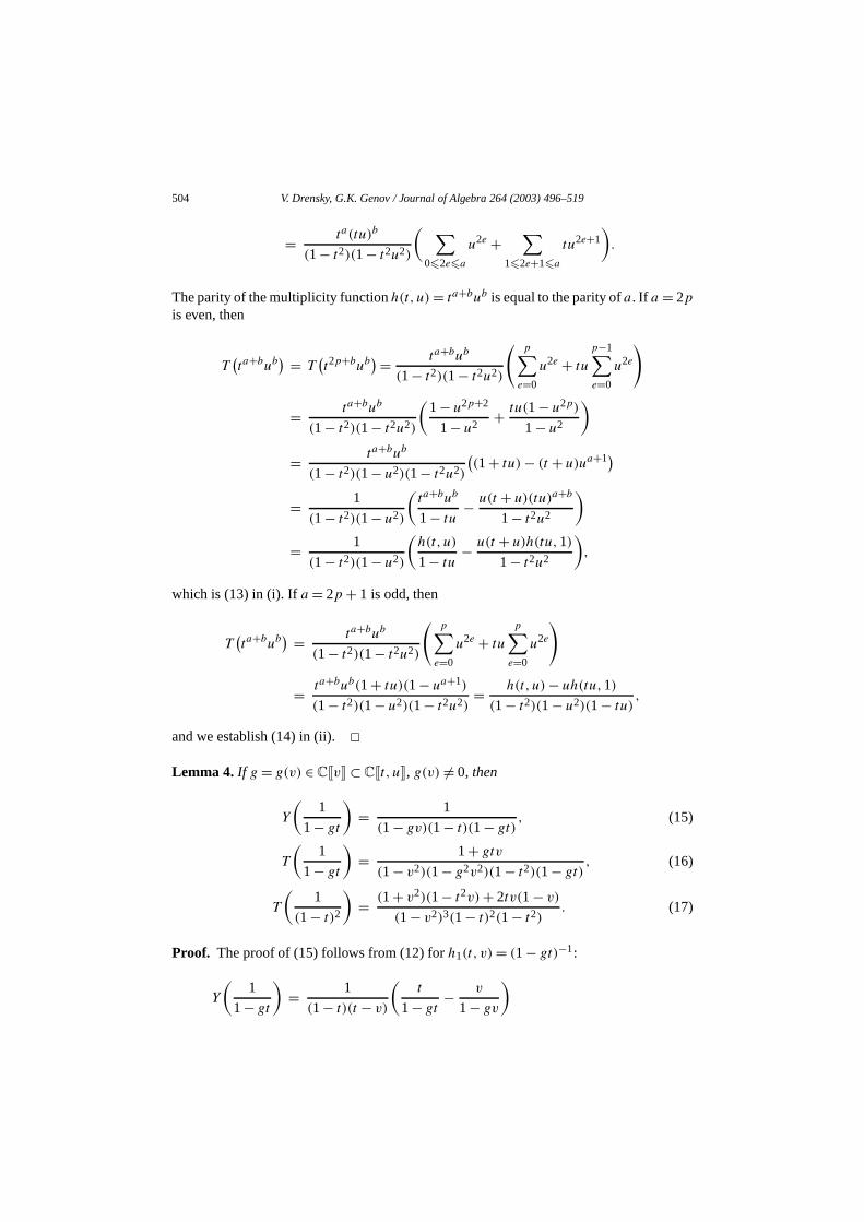
504 V. Drensky, G.K. Genov / Journal of Algebra 264 (2003) 496–519
= ta(tu)b
(1− t2)(1− t2u2)
( ∑02ea
u2e +∑
12e+1a
tu2e+1).
The parity of the multiplicity functionh(t, u)= ta+bub is equal to the parity ofa. If a = 2pis even, then
T(ta+bub
) = T(t2p+bub
)= ta+bub
(1− t2)(1− t2u2)
(p∑e=0
u2e + tu
p−1∑e=0
u2e
)
= ta+bub
(1− t2)(1− t2u2)
(1− u2p+2
1− u2+ tu(1− u2p)
1− u2
)
= ta+bub
(1− t2)(1− u2)(1− t2u2)
((1+ tu)− (t + u)ua+1)
= 1
(1− t2)(1− u2)
(ta+bub
1− tu− u(t + u)(tu)a+b
1− t2u2
)
= 1
(1− t2)(1− u2)
(h(t, u)
1− tu− u(t + u)h(tu,1)
1− t2u2
),
which is (13) in (i). Ifa = 2p + 1 is odd, then
T(ta+bub
) = ta+bub
(1− t2)(1− t2u2)
(p∑e=0
u2e + tu
p∑e=0
u2e
)
= ta+bub(1+ tu)(1− ua+1)
(1− t2)(1− u2)(1− t2u2)= h(t, u)− uh(tu,1)
(1− t2)(1− u2)(1− tu),
and we establish (14) in (ii). Lemma 4. If g = g(v) ∈ Cv ⊂ Ct, u, g(v) = 0, then
Y
(1
1− gt
)= 1
(1− gv)(1 − t)(1− gt), (15)
T
(1
1− gt
)= 1+ gtv
(1− v2)(1− g2v2)(1− t2)(1− gt), (16)
T
(1
(1− t)2
)= (1+ v2)(1− t2v)+ 2tv(1 − v)
(1− v2)3(1− t)2(1− t2). (17)
Proof. The proof of (15) follows from (12) forh1(t, v)= (1− gt)−1:
Y
(1
)= 1
(t − v
)
1− gt (1− t)(t − v) 1− gt 1− gv
V. Drensky, G.K. Genov / Journal of Algebra 264 (2003) 496–519 505
= 1
(1− gv)(1 − t)(1− gt)(t − v)
(t (1− gv)− v(1 − gt)
)
= t − v
(1− gv)(1 − t)(1− gt)(t − v)= 1
(1− gv)(1 − t)(1− gt).
For (16) we separate the even and odd parts ofh(t, u)= h1(t, v)= (1− gt)−1:
h(t, u)= 1
1− gt= 1+ gt
1− g2t2, heven(t, u)= 1
1− g2t2, hodd(t, u)= gt
1− g2t2,
use thath(tu,1)= h1(v, v) and apply Proposition 3. Direct calculations give
T(heven(t, u)
) = 1
(1− t2)(1− u2)
(1
(1− v)(1 − g2t2)− u(t + u)
(1− v2)(1− g2v2)
)
= 1+ g2t2v
(1− v2)(1− g2v2)(1− t2)(1− g2t2),
T(hodd(t, u)
) = 1
(1− t2)(1− v)(1 − u2)
(gt
1− g2t2− gtu2
1− g2v2
)
= gt
(1− v)(1 − g2v2)(1− t2)(1− g2t2),
T(h(t, u)
) = (1+ g2t2v)+ gt (1+ v)
(1− v2)(1− g2v2)(1− t2)(1− g2t2)
= (1+ gt)(1 + gtv)
(1− v2)(1− g2v2)(1− t2)(1− g2t2)
= 1+ gtv
(1− v2)(1− g2v2)(1− t2)(1− gt).
The proof of (17) is similar and uses that for
h(t)= 1
(1− t)2= (1+ t2)+ 2t
(1− t2)2,
heven(t)= 1+ t2
(1− t2)2, hodd(t)= 2t
(1− t2)2.

506 V. Drensky, G.K. Genov / Journal of Algebra 264 (2003) 496–519
s of
3. Main results
First we shall find the multiplicities of the Schur functions in the Hilbert serieC[W(3,0)]
Hilb(C[W(3,0)
], x, y
) = 1
(1− x3)(1− x2y)(1− xy2)(1− y3)
=∑p,q0
k(p, q)xpyq =∑λ
m(λ)Sλ(x, y). (18)
As usually, we denote by #P the number of elements of the finite setP and byN0 the setof nonnegative integers.
Lemma 5. Let λ= (λ1, λ2)= (p, q), p q 0, and let
Aλ = (a1, b1, c1,0) ∈ N
40
∣∣ 3a1 + 2b1 + c1 = p, b1 + 2c1 = q, (19)
Bλ = (a2, b2,0, d2) ∈ N
40
∣∣ 3a2 + 2b2 = p + 1, b2 + 3d2 = q − 1
(20)
(where Bp0 = ∅). Then the multiplicity m(λ) in (18) is equal to #Aλ − #Bλ.
Proof. Since
1
(1− x3)(1− x2y)(1− xy2)(1− y3)=∑a0
(x3)a∑
b0
(x2y
)b∑c0
(xy2)c∑
d0
(y3)d
=∑
a,b,c,d0
x3a+2b+cyb+2c+3d,
the coefficientk(p, q) is equal to the number of solutions(a, b, c, d) in nonnegativeintegers of the system of two equations
3a + 2b+ c = p, b + 2c+ 3d = q.
We fix λ= (p, q) and consider the sets
A= (a1, b1, c1, d1) ∈ N
40
∣∣ 3a1 + 2b1 + c1 = p, b1 + 2c1 + 3d1 = q,
B = (a2, b2, c2, d2) ∈ N
40
∣∣ 3a2 + 2b2 + c2 = p+ 1, b2 + 2c2 + 3d2 = q − 1
(whereB = ∅ if q = 0). Clearly,k(p, q)= #A andk(p + 1, q − 1)= #B. Hence, by (2),
m(λ)= k(p, q)− k(p + 1, q − 1)= #A− #B.
We present the setsA andB as disjoint unions
A=Aλ ∪A+, B = Bλ ∪B+,

V. Drensky, G.K. Genov / Journal of Algebra 264 (2003) 496–519 507
of3. Let
where
A+ = (a1, b1, c1, d1) ∈A | d1 > 0
, B+ =
(a2, b2, c2, d2) ∈B | c2 > 0.
For every quadruple(a1, b1, c1, d1) ∈ A+ and 3a1 + 2b1 + c1 = p, b1 + 2c1 + 3d1 = q ,we obtain that 3a1 + 2b1 + (c1 + 1)= p + 1, b1 + 2(c1 + 1)+ 3(d1 − 1)= q − 1. Sinced1 > 0, we obtain that(a2, b2, c2, d2)= (a1, b1, c1+1, d1−1) belongs toB+. Similarly, if(a2, b2, c2, d2) ∈ B+, then(a1, b1, c1, d1)= (a2, b2, c2 − 1, d2 + 1) belongs toA+. Hence,the mappingA+ →B+ defined by(a1, b1, c1, d1)→ (a1, b1, c1 + 1, d1 − 1) is a bijectionand
m(λ)= #(Aλ ∪A+)− #
(Bλ ∪B+)= (#Aλ − #Bλ)− (
#A+ − #B+)= #Aλ − #Bλ. Corollary 6. Let λ= (λ1, λ2)= (p, q), p q 0, and let m(λ) be the multiplicity in (18).If 3 does not divide p + q , then m(λ) = 0. If p + q is divisible by 3 and p + q = 3r forsome r ∈ N0, then
m(λ) = #
([2q − p
3,q
2
]∩ N0
)− #
([2q − p− 3
6,q − 1
3
]∩ N0
)
= #
([q − r,
q
2
]∩ N0
)− #
([q − r − 1
2,q − 1
3
]∩ N0
),
i.e., m(λ) is equal to the difference of the numbers of nonnegative integers in the intervals[2p− q
3,q
2
]=[q − r,
q
2
]and
[2q − p− 3
6,q − 1
3
]=[q − r − 1
2,q − 1
3
].
Proof. Clearly,m(λ) = 0 if p + q = λ1 + λ2 is not divisible by 3 because the degreesthe homogeneous components of the symmetric function in (18) are multiples ofp + q = 3r. By Lemma 5, we have to find the number of elements in the setsAλ andBλ
in (19) and (20), respectively, i.e., the number of solutions inN30 of the systems
3a1 + 2b1 + c1 = p, b1 + 2c1 = q, (21)
3a2 + 2b2 = p + 1, b2 + 3d2 = q − 1. (22)
The solutions of (21) are the triples of integers(a1, b1, c1), where
b1 = q − 2c1 0,
a1 = p − 2b1 − c1
3= (3r − q)− 2(q − 2c1)− c1
3= r − q + c1 0.
Hencec1 satisfies the conditions
c1 0, c1 q − r, c1 q
2
508 V. Drensky, G.K. Genov / Journal of Algebra 264 (2003) 496–519
in the
ilarly.
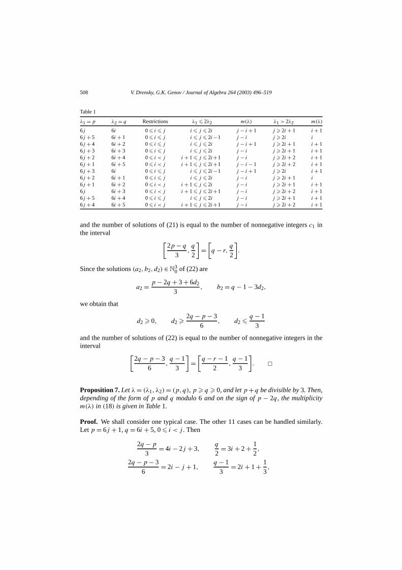
Table 1
λ1 = p λ2 = q Restrictions λ1 2λ2 m(λ) λ1 > 2λ2 m(λ)
6j 6i 0 i j i j 2i j − i + 1 j 2i + 1 i + 16j + 5 6i + 1 0 i j i j 2i−1 j − i j 2i i
6j + 4 6i + 2 0 i j i j 2i j − i + 1 j 2i + 1 i + 16j + 3 6i + 3 0 i j i j 2i j − i j 2i + 1 i + 16j + 2 6i + 4 0 i < j i + 1 j 2i+1 j − i j 2i + 2 i + 16j + 1 6i + 5 0 i < j i + 1 j 2i+1 j − i − 1 j 2i + 2 i + 16j + 3 6i 0 i j i j 2i−1 j − i + 1 j 2i i + 16j + 2 6i + 1 0 i j i j 2i j − i j 2i + 1 i
6j + 1 6i + 2 0 i < j i + 1 j 2i j − i j 2i + 1 i + 16j 6i + 3 0 i < j i + 1 j 2i+1 j − i j 2i + 2 i + 16j + 5 6i + 4 0 i j i j 2i j − i j 2i + 1 i + 16j + 4 6i + 5 0 i < j i + 1 j 2i+1 j − i j 2i + 2 i + 1
and the number of solutions of (21) is equal to the number of nonnegative integersc1 inthe interval [
2p− q
3,q
2
]=[q − r,
q
2
].
Since the solutions(a2, b2, d2) ∈ N30 of (22) are
a2 = p − 2q + 3+ 6d2
3, b2 = q − 1− 3d2,
we obtain that
d2 0, d2 2q − p − 3
6, d2 q − 1
3
and the number of solutions of (22) is equal to the number of nonnegative integersinterval [
2q − p − 3
6,q − 1
3
]=[q − r − 1
2,q − 1
3
].
Proposition 7. Let λ= (λ1, λ2)= (p, q), p q 0, and let p+ q be divisible by 3. Then,depending of the form of p and q modulo 6 and on the sign of p − 2q , the multiplicitym(λ) in (18) is given in Table 1.
Proof. We shall consider one typical case. The other 11 cases can be handled simLet p = 6j + 1, q = 6i + 5, 0 i < j . Then
2q − p
3= 4i − 2j + 3,
q
2= 3i + 2+ 1
2,
2q − p− 3 = 2i − j + 1,q − 1 = 2i + 1+ 1
,
6 3 3
V. Drensky, G.K. Genov / Journal of Algebra 264 (2003) 496–519 509
ervalsre
isrs
eachcase
Table 2
No. λ1 = p λ2 = q Restrictions gn,i(t, u)
1 6j 6i 0 i j (1− t6(i+1))
2 6j + 5 6i + 1 0 i j t11u(1− t6i )
3 6j + 4 6i + 2 0 i j t4u2(1− t6(i+1))
4 6j + 3 6i + 3 0 i j t9u3(1− t6(i+1))
5 6j + 2 6i + 4 0 i < j t8u4(1− t6(i+1))
6 6j + 1 6i + 5 0 i < j t13u5(1− t6(i+1))
7 6j + 3 6i 0 i j t3(1− t6(i+1))
8 6j + 2 6i + 1 0 i j t8u(1− t6i )
9 6j + 1 6i + 2 0 i < j t7u2(1− t6(i+1))
10 6j 6i + 3 0 i < j t6u3(1− t6(i+1))
11 6j + 5 6i + 4 0 i j t11u4(1− t6(i+1))
12 6j + 4 6i + 5 0 i < j t10u5(1− t6(i+1))
and by Corollary 6 we need to find the number of nonnegative integers in the int[4i − 2j + 3,3i + 2 + 1/2] and [2i − j + 1,2i + 1 + 1/3]. Clearly, these numbers athe same as for the intervals[4i − 2j + 3,3i + 2] and[2i − j + 1,2i + 1]. The conditionλ1 λ2 0, i.e.,p q 0, is equivalent toj > i 0.
The caseλ1 2λ2, i.e.,p 2q , holds for 6j + 1 12i + 10 andj 2i + 1 + 1/2.We work with integers, this means thati + 1 j 2i + 1. Since 4i − 2j + 3 > 0,the integers in the interval[4i − 2j + 3,3i + 2] are positive and their number#Aλ = (3i + 2) − (4i − 2j + 3) + 1 = 2j − i. The number of nonnegative integein [2i − j + 1,2i + 1] is equal to #Bλ = (2i + 1) − (2i − j + 1) + 1 = j + 1 andm(λ)= #Aλ − #Bλ = (2j − i)− (j + 1)= j − i − 1.
If λ1 > 2λ2 (i.e., p > 2q), then [4i − 2j + 3,3i + 2] ∩ N0 = [0,3i + 2] ∩ N0 and[2i − j + 1,2i + 1] ∩ N0 = [0,2i + 1] ∩ N0. Hence the number of elements ofAλ andBλ
is equal to 3i + 3 and 2i + 2, respectively, andm(λ)= (3i + 3)− (2i + 2)= i + 1. Lemma 8. The multiplicity series of the symmetric function in (18) is
M(Hilb
(C[W(3,0)
], x, y
))=∑i0
(tu)6i
(1− t6)2
12∑n=1
gn,i (t, u). (23)
The twelve functions gn,i(t, u) are given in Table 2 and are of the form g(t, u)= tαuβ(1−t6(i+δ)), where α,β are integers and δ = 0,1.
Proof. By Proposition 7,
M(Hilb
(C[W(3,0)
], x, y
))=∑q0
(∑pq
m(p,q)tpuq),
wherem(p,q) are taken from Table 1. The twelve summands in (23) correspond torow of this table. Again, as in the proof of Proposition 7, we shall consider only the

510 V. Drensky, G.K. Genov / Journal of Algebra 264 (2003) 496–519
ing
p = 6j+1,q = 6i+5, 0 i < j . The other 11 cases are similar. We perform the followcalculations with the sum:h6,i(t, u) =∑j>i
m(6j + 1,6i + 5)t6j+1u6i+5
= u6i+5
(2i+1∑j=i+1
(j − i − 1)t6j+1 +∑
j2i+2
(i + 1)t6j+1
)
= t6i+13u6i+5
(i∑
j=0
(j + 1)t6j + (i + 1)∑
ji+1
t6j
)
= t6i+13u6i+5
(i∑
j=0
(j + 1)t6j +( ∑ji+1
(j + 1)t6j − t6(i+1)∑j0
(j + 1)t6j))
= t6i+13u6i+5∑j0
(j + 1)t6j(1− t6(i+1))= t6i+13u6i+5(1− t6(i+1))
(1− t6)2,
h6,i(t, u) = (tu)6i
(1− t6)2g6,i(t, u), g6,i(t, u)= t13u5(1− t6(i+1)).
The following theorem is one of the main results of the paper.
Theorem 9. The multiplicity series of the Hilbert series of C[W(3,0)] are the following:
M(Hilb
(C[W(3,0)
], x, y
))(t, u) = M
(1
(1− x3)(1− x2y)(1− xy2)(1− y3)
)(t, u)
= 1− t2u+ t4u2
(1− t3)(1− t6u6)(1− t2u), (24)
M ′(Hilb(C[W(3,0)
], x, y
))(t, v) = 1− tv + t2v2
(1− t3)(1− v6)(1− tv). (25)
Proof. It is sufficient to evaluate the sum (23). LetM =M(Hilb(C[W(3,0)], x, y))(t, u).Then, by Lemma 8,
M = 1
(1− t6)2
∑i0
(tu)6ign,i (t, u)
= 1
(1− t6)2
(w1(t, u)
∑i0
(tu)6i −w2(t, u)∑i0
(t2u)6i)
= 16 2
(w1(t, u)
6− w2(t, u)
2 6
),
(1− t ) 1− (tu) 1− (t u)

V. Drensky, G.K. Genov / Journal of Algebra 264 (2003) 496–519 511
re forknow
wherew1(t, u) andw2(t, u) are obtained from the data in Table 2 and
w1(t, u) = 1+ t11u+ t4u2 + t9u3 + t8u4 + t13u5 + t3 + t8u+ t7u2 + t6u3 + t11u4
+ t10u5
= (1+ t3
)(1+ t8u+ t4u2 + t6u3 + t8u4 + t10u5)
= (1+ t3
)((1+ t2u+ (
t2u)2 + (
t2u)3 + (
t2u)4 + (
t2u)5)+ (
t8u− t2u))
= (1+ t3
)(1− (t2u)6
1− t2u− t2u
(1− t6
)),
w2(t, u) = t6 + t11u+ t10u2 + t15u3 + t14u4 + t19u5 + t9 + t8u+ t13u2 + t12u3
+ t17u4 + t16u5
= (1+ t3
)t6(1+ t2u+ (
t2u)2 + (
t2u)3 + (
t2u)4 + (
t2u)5)
= (1+ t3)(1− (t2u)6)t6
1− t2u.
Therefore
M = 1+ t3
(1− t6)2
(1
1− (tu)6
(1− (t2u)6
1− t2u− t2u
(1− t6
))− t6
1− t2u
)
= 1− (t2u)6 − t2u(1− t6)(1− t2u)− t6(1− (tu)6)
(1− t3)(1− t6)(1− (tu)6)(1− t2u)
= (1− t6)(1− t2u+ t4u2)
(1− t3)(1− t6)(1− (tu)6)(1− t2u),
which gives (24). Formula (25) is obtained from (24) by the substitutionu= v/t . Lemma 10. The function M ′(t, v) = M ′(Hilb(C[W(3,0)], x, y))(t, v) from (25) can bepresented in the form
M ′(t, v)= 1
1− v3
(a1
1− t+ a2
1−ωt+ a3
1−ω2t+ a4
1− tv
), (26)
where ω = 12(−1+ i
√2) is a primitive cubic root of unity,
a1 = 1
3(1− v2), a2 = 1
3(1−ωv2), a3 = 1
3(1−ω2v2), a4 = −v3
1− v6 .
Proof. We may consider the functionM ′(t, v) as a rational function int with coefficientsin C(v). Then the decomposition (26) can be found using the standard procedupresenting a rational function as a sum of elementary fractions. (Or, if we alreadythe coefficientsa1, a2, a3, a4 ∈ C(v), we can check (26) directly.)

512 V. Drensky, G.K. Genov / Journal of Algebra 264 (2003) 496–519
ratione
In the sequel, we prefer to keep the denominators of rational functions in consideas products of factors in the form 1− ta , 1 − vb , 1 − tavb instead to make somcancellations, because this form is convenient for asymptotic estimates.
Lemma 11. The application of the operators T and Y to the multiplicity series M ′(t, v)=M ′(Hilb(C[W(3,0)], x, y))(t, v) gives
T Y(M ′(t, v)
)= 1
(1− v3)(1− v6)
((1+ v2 + v4)((1+ v2)(1− t2v)+ 2tv(1− v))
3(1− v)(1 − v2)3(1− t)2(1− t2)
+ (1− v)(1+ tv)
3(1− v2)(1− t)(1− t2)+ (1− v2)(1− tv)
3(1− v3)(1− t3)
− v3((1− v + v2)(1− t2v2)+ tv(1 − v2))
(1− v)(1 − v2)2(1− v4)(1− t)(1− t2)(1− tv)
).
Proof. Applying Lemma 1(i) and Lemma 4 to (26), we obtain
Y(M ′(t, v)
) = 1
1− v3
(a1Y
(1
1− t
)+ a2Y
(1
1−ωt
)+ a3Y
(1
1−ω2t
)
+ a4Y
(1
1− tv
))
= 1
(1− v3)(1− t)
(a1
(1− v)(1− t)+ a2
(1−ωv)(1−ωt)
+ a3
(1−ω2v)(1−ω2t)+ a4
(1− v2)(1− tv)
).
We use that
1
(1− t)(1−ωt)= 1
1−ω
(1
1− t− ω
1−ωt
)
and presentY (M ′(t, v)) in the form
Y(M ′(t, v)
)= 1
1− v3
(a1
(1− v)(1− t)2
+(
a2
(1−ω)(1−ωv)+ a3
(1−ω2)(1−ω2v)
)1
1− t
− a2ω
(1−ω)(1−ωv)(1 −ωt)− a3ω
2
(1−ω2)(1−ω2v)(1−ω2t)
+ a42
).
(1− v )(1− tv)

V. Drensky, G.K. Genov / Journal of Algebra 264 (2003) 496–519 513
f the
rmals of
s.
Now the proof is completed by applying again Lemmas 1(i) and 4, replacinga1, a2, a3, a4with their expressions from Lemma 10 and using that(1−ωz)(1−ω2z)= 1+ z+ z2.
The next theorem is the main result of the paper and gives the explicit form omultiplicity series for the algebra of invariants of two 3× 3 matrices.
Theorem 12. The multiplicity series of the Hilbert series of the algebra C2,3 of invariantsof two 3× 3 matrices is
M ′(Hilb(C2,3, x, y))(t, v)
= 1
(1− v2)(1− v3)2
((1+ v2 + v4)((1+ v2)(1− t2v)+ 2tv(1 − v))
3(1− v)(1− v2)3(1− t)2(1− t2)
+ (1− v)(1+ tv)
3(1− v2)(1− t)(1− t2)+ (1− v2)(1− tv)
3(1− v3)(1− t3)
− v3((1− v + v2)(1− t2v2)+ tv(1 − v2))
(1− v)(1− v2)2(1− v4)(1− t)(1− t2)(1− tv)
).
Proof. Applying Lemma 1(i) to the symmetric function (5) we obtain
M ′(Hilb(C2,3, x, y))(t, v)= 1+ v3
1− v2T Y(M ′(Hilb
(C[W(3,0)
], x, y
))(t, v)
)and the result follows immediately from Lemma 11.Remark 13. Using (11), one can check directly (even without computer) that the fopower series int, u or in t, v from Theorems 9 and 12 are equal to the multiplicity seriethe symmetric functions Hilb(C[W(3,0)], x, y) and Hilb(C2,3, x, y), respectively. In thisway, the main difficulties are how to find the right candidates for the multiplicity serie
4. Asymptotic behavior of invariants of two 3 × 3 matrices
In this section we shall determine the exact asymptotics of the multiplicities ofSλ(x, y)
in the Hilbert series of the algebra of invariants of two 3× 3 matrices. Using MAPLE wehave found the following expression for the multiplicity seriesM ′(Hilb(C2,3, x, y))(t, v):
M ′(Hilb(C2,3, x, y))(t, v) = h1(v)
1− t+ h2(v)
(1− t)2+ h3(v)
(1− t)3+ h4(v)
1+ t+ h5(v)+ h6(v)t
1+ t + t2
+ h7(v), (27)
1− tv

514 V. Drensky, G.K. Genov / Journal of Algebra 264 (2003) 496–519
where
h1(v) = (1− v + v2)(17− 26v − 49v2 + 32v3 + 160v4 + 32v5 − 49v6 − 26v7 + 17v8)
72(1− v)8(1+ v)4(1+ v + v2)3,
h2(v) = (1− v + v2)(3− v − 2v2 + v3 + 5v4)
12(1− v)7(1+ v)3(1+ v + v2)2,
h3(v) = 1− v + v2
6(1− v)6(1+ v)2(1+ v + v2), h4(v)= 1
8(1− v)2(1+ v)4(1+ v2),
h5(v) = 2+ v
9(1− v3)3, h6(v)= 1− v
9(1− v3)3,
h7(v) = −v6
(1− v)8(1+ v)4(1+ v + v2)2(1+ v2).
We need the following easy lemma.
Lemma 14. Let f (z), g(z) ∈ C[z] be two polynomials such that f (1), g(1) = 0, and let
f (z)
(1− z)kg(z)= a0
(1− z)k+ a1
(1− z)k−1 + · · · + ak−1
1− z+ b(z)
g(z)+ c(z) (28)
for some constants a0, a1, . . . , ak−1 and some polynomials b(z), c(z). Then
a0 = f (1)
g(1).
Proof. Using (28) we obtain
(a0 + a1(1− z)+ · · · + ak−1(1− z)k−1)g(z)+ b(z)(1− z)k + c(z)g(z)(1− z)k = f (z).
Hence forz= 1 we havea0g(1)= f (1) which completes the proof.Theorem 15. Let
M ′(Hilb(C2,3, x, y))(t, v)=
∑λ=(p,q)
m(p,q)tp−qvq
and let n= p + q . Then for p > 2q 0
m(p,q) = q7
7!2532+ (p − q)q6
6!2432+ (p − q)2q5
2!5!2332+O
(n6)
= p2q5
17280− 11pq6
103680+ 71q7
1451520+O
(n6)
and for 2q p q 0

V. Drensky, G.K. Genov / Journal of Algebra 264 (2003) 496–519 515
f
m(p,q) = q7
7!2532+ (p− q)q6
6!2432+ (p− q)2q5
2!5!2332− (2q − p)7
7!2532+O
(n6)
= p7
1451520− p6q
103680+ p5q2
17280− p4q3
5184+ p3q4
2592− 7p2q5
17280+ 7pq6
34560− 19q7
483840
+O(n6).
Proof. We make use of the fact that if|a| = 1, then in the expression
1
(1− az)k+1=∑n0
pntn =
∑n0
(n+ k
k
)antn
the coefficientspn satisfy
pn = annk
k! +O(nk−1).
Presenting the multiplicity series ofM ′(Hilb(C2,3, x, y))(t, v) in (27) as a sum oelementary fractions we obtain summands of the form
1
1− t
(8∑
k=1
a8−k,1(1− v)k
+4∑
k=1
a4−k,−1
(1+ v)k+
3∑k=1
a3−k,ω(1−ωv)k
+3∑
k=1
a3−k,ω2
(1−ω2v)k
),
1
(1− t)2
(7∑
k=1
b7−k,1(1− v)k
+3∑
k=1
b3−k,−1
(1+ v)k+
2∑k=1
b2−k,ω(1−ωv)k
+2∑
k=1
b2−k,ω2
(1−ω2v)k
),
1
(1− t)3
(6∑
k=1
c6−k,1(1− v)k
+2∑
k=1
c2−k,−1
(1+ v)k+ c0,ω
1−ωv+ c0,ω2
1−ω2v
),
1
1+ t
(2∑
k=1
d2−k,1(1− v)k
+4∑
k=1
d4−k,−1
(1+ v)k+ c0,i
1− iv+ c0,−i
1+ iv
),
1
1−ωt
(3∑
k=1
e3−k,1(1− v)k
+3∑
k=1
e3−k,ω(1−ωv)k
+3∑
k=1
e3−k,ω2
(1−ω2v)k
),
1
1−ω2t
(3∑
k=1
f3−k,1(1− v)k
+3∑
k=1
f3−k,ω(1−ωv)k
+3∑
k=1
f3−k,ω2
(1−ω2v)k
),
1
1− tv
(8∑
k=1
g8−k,1(1− v)k
+4∑
k=1
g4−k,−1
(1+ v)k
+2∑ g2−k,ω
(1−ωv)k+
2∑ g2−k,ω2
(1−ω2v)k+ g0,i
1− iv+ g0,−i
1+ iv
),
k=1 k=1
516 V. Drensky, G.K. Genov / Journal of Algebra 264 (2003) 496–519
the
to
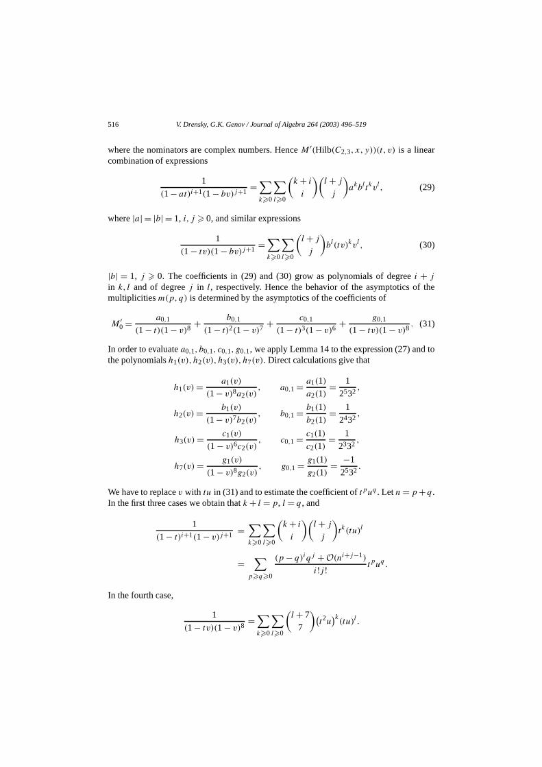
where the nominators are complex numbers. HenceM ′(Hilb(C2,3, x, y))(t, v) is a linearcombination of expressions
1
(1− at)i+1(1− bv)j+1 =∑k0
∑l0
(k + i
i
)(l + j
j
)akbltkvl, (29)
where|a| = |b| = 1, i, j 0, and similar expressions
1
(1− tv)(1 − bv)j+1 =∑k0
∑l0
(l + j
j
)bl(tv)kvl , (30)
|b| = 1, j 0. The coefficients in (29) and (30) grow as polynomials of degreei + j
in k, l and of degreej in l, respectively. Hence the behavior of the asymptotics ofmultiplicitiesm(p,q) is determined by the asymptotics of the coefficients of
M ′0 = a0,1
(1− t)(1− v)8+ b0,1
(1− t)2(1− v)7+ c0,1
(1− t)3(1− v)6+ g0,1
(1− tv)(1 − v)8. (31)
In order to evaluatea0,1, b0,1, c0,1, g0,1, we apply Lemma 14 to the expression (27) andthe polynomialsh1(v), h2(v), h3(v), h7(v). Direct calculations give that
h1(v)= a1(v)
(1− v)8a2(v), a0,1 = a1(1)
a2(1)= 1
2532 ,
h2(v)= b1(v)
(1− v)7b2(v), b0,1 = b1(1)
b2(1)= 1
2432,
h3(v)= c1(v)
(1− v)6c2(v), c0,1 = c1(1)
c2(1)= 1
2332,
h7(v)= g1(v)
(1− v)8g2(v), g0,1 = g1(1)
g2(1)= −1
2532 .
We have to replacev with tu in (31) and to estimate the coefficient oftpuq . Letn= p+q .In the first three cases we obtain thatk + l = p, l = q , and
1
(1− t)i+1(1− v)j+1 =∑k0
∑l0
(k + i
i
)(l + j
j
)tk(tu)l
=∑
pq0
(p− q)iqj +O(ni+j−1)
i!j ! tpuq.
In the fourth case,
1
(1− tv)(1 − v)8=∑∑(
l + 7
7
)(t2u)k(tu)l .
k0 l0
V. Drensky, G.K. Genov / Journal of Algebra 264 (2003) 496–519 517
(5) is
981].
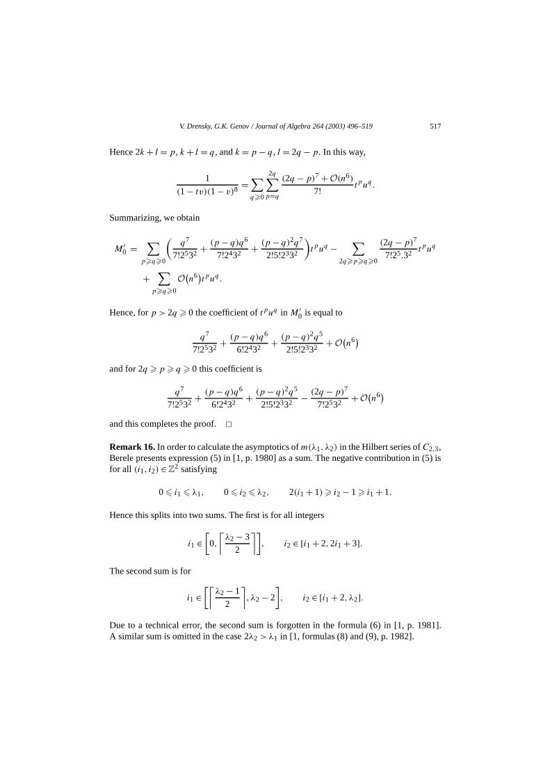
Hence 2k + l = p, k + l = q , andk = p − q , l = 2q − p. In this way,
1
(1− tv)(1− v)8=∑q0
2q∑p=q
(2q − p)7 +O(n6)
7! tpuq.
Summarizing, we obtain
M ′0 =
∑pq0
(q7
7!2532 + (p− q)q6
7!2432 + (p− q)2q7
2!5!2332
)tpuq −
∑2qpq0
(2q − p)7
7!25.32 tpuq
+∑
pq0
O(n6)tpuq.
Hence, forp > 2q 0 the coefficient oftpuq in M ′0 is equal to
q7
7!2532 + (p − q)q6
6!2432 + (p − q)2q5
2!5!2332 +O(n6)
and for 2q p q 0 this coefficient is
q7
7!2532 + (p − q)q6
6!2432 + (p − q)2q5
2!5!2332 − (2q − p)7
7!2532 +O(n6)
and this completes the proof.Remark 16. In order to calculate the asymptotics ofm(λ1, λ2) in the Hilbert series ofC2,3,Berele presents expression (5) in [1, p. 1980] as a sum. The negative contribution infor all (i1, i2) ∈ Z2 satisfying
0 i1 λ1, 0 i2 λ2, 2(i1 + 1) i2 − 1 i1 + 1.
Hence this splits into two sums. The first is for all integers
i1 ∈[0,
⌈λ2 − 3
2
⌉], i2 ∈ [i1 + 2,2i1 + 3].
The second sum is for
i1 ∈[⌈
λ2 − 1
2
⌉, λ2 − 2
], i2 ∈ [i1 + 2, λ2].
Due to a technical error, the second sum is forgotten in the formula (6) in [1, p. 1A similar sum is omitted in the case 2λ2 > λ1 in [1, formulas (8) and (9), p. 1982].

518 V. Drensky, G.K. Genov / Journal of Algebra 264 (2003) 496–519
ven
mialef
5. Symmetric functions in more than two variables
By analogy with the multiplicity seriesM(f )(t, u) of the symmetric functionf (x, y) ∈Symx, y, we can introduce the multiplicity series of symmetric functions in any (einfinite) number of variables. Iff (x1, . . . , xk) ∈ Cx1, . . . , xk is a symmetric function ink variables, thenf has a presentation
f (x1, . . . , xk)=∑
m(λ)Sλ(x1, . . . , xk),
where the summation runs on all partitionsλ = (λ1, . . . , λk). We define the multiplicityseries as
M(f )(t1, . . . , tk)=∑
m(λ)tλ11 · · · tλkk .
Using the Young rule it is easy to prove the following analogue of Proposition 2.
Proposition 17.
Y(M(f )
) = M
(f (x1, . . . , xk)
(1− x1) · · · (1− xk)
)
=k∏
i=1
1
1− ti
∑(−t2)
ε2 · · · (−tk)εkM(f )
(t1t
ε22 , t
1−ε22 t
ε33 , . . . , t
1−εk−1k−1 t
εkk , t
1−εkk
),
where the summation runs on all ε2, . . . , εk = 0,1.
In the special casek = 2 we obtain
Y(M(f (x1, x2)
)) = M
(f (x1, x2)
(1− x1)(1− x2)
)
= 1
(1− t1)(1− t2)
(M(f )(t1, t2)− t2M(f )(t1t2,1)
),
which is (12).The above formalism allows to write in a compact form some results on polyno
identities and invariants of 2× 2 matrices. For example, ifTk,2 is the algebra with tracgenerated byk generic 2× 2 matrices, andCk,2 is the center ofTk,2, then the results oProcesi [7] and Formanek [4] can be written in the form
Hilb(Tk,2, x1, . . . , xk)
=k∏
i=1
1
1− xi
∑S(µ1,µ2,µ3)(x1, . . . , xk)
=∑
(λ1 − λ2 + 1)(λ2 − λ3 + 1)(λ3 − λ4 + 1)S(λ1,λ2,λ3,λ4)(x1, . . . , xk),

V. Drensky, G.K. Genov / Journal of Algebra 264 (2003) 496–519 519
rix
trices,
984)
.
in, DC.
econd
Math.
Hilb(Ck,2, x1, . . . , xk)=k∏
i=1
1
1− xi
∑ab0
∑c0
S(2a+c,2b+c,c)(x1, . . . , xk),
and this implies that
M(Hilb(Tk,2, x1, . . . , xk)
) = Y
(1
(1− t1)(1− t1t2)(1− t1t2t3)
)
= 1
(1− t1)2(1− t1t2)2(1− t1t2t3)2(1− t1t2t3t4),
M(Hilb(Ck,2, x1, . . . , xk)
) = Y
(1
(1− t21)(1− (t1t2)2)(1− t1t2t3)
).
The results for the polynomial identities of 2× 2 algebras in terms of the generic matalgebra and its center, as given in [2,4,7] can be stated in a similar way.
Acknowledgment
The authors are very thankful to Irina Genova for her help with MAPLE.
References
[1] A. Berele, Approximate multiplicities in the trace cocharacter sequence of two three-by-three maComm. Algebra 25 (1997) 1975–1983.
[2] V. Drensky, Codimensions ofT -ideals and Hilbert series of relatively free algebras, J. Algebra 91 (11–17.
[3] V. Drensky, G.K. Genov, Multiplicities of Schur functions in invariants of two 3× 3 matrices, C. R. AcadBulg. Sci. 55 (6) (2002) 5–10.
[4] E. Formanek, Invariants and the ring of generic matrices, J. Algebra 89 (1984) 178–223.[5] E. Formanek, The Polynomial Identities and Invariants ofn× n Matrices. CBMS Regional Conf. Series
Math., Vol. 78, AMS, Providence, RI, 1991. Published for Confer. Board of the Math. Sci., Washington[6] I.G. Macdonald, Symmetric Functions and Hall Polynomials, Oxford Univ. Press, Oxford, 1979, S
edition, 1995.[7] C. Procesi, Computing with 2× 2 matrices, J. Algebra 87 (1984) 342–359.[8] A. Regev, Young-derived sequences ofSn-characters, Adv. Math. 106 (1994) 169–197.[9] Y. Teranishi, The ring of invariants of matrices, Nagoya Math. J. 104 (1986) 149–161.
[10] R.M. Thrall, On symmetrized Kronecker powers and the structure of the free Lie ring, Trans. Amer.Soc. 64 (1942) 371–388.