Chapter 3 1

Chapter 3:

Laplace Transform

Chapter 3 [2]

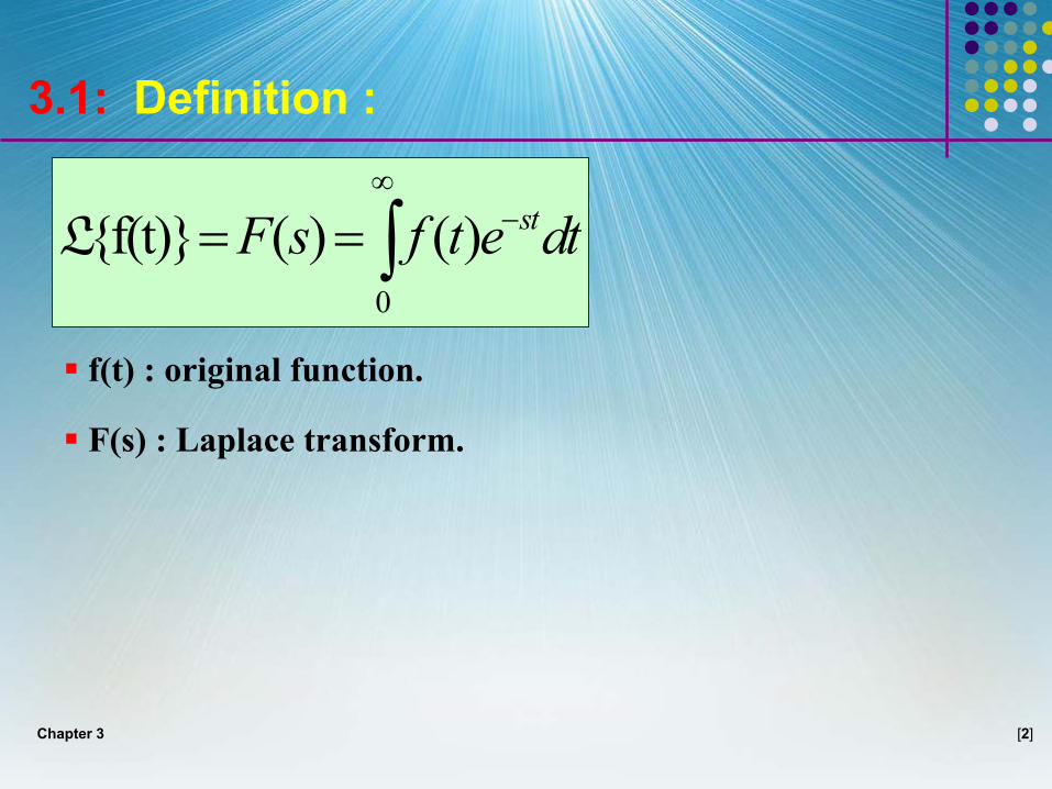
3.1: Definition :

0

{f(t)} ( ) ( )∞

−= =∫ stF s f t e dtL

f(t) : original function.

F(s) : Laplace transform.

Chapter 3 [3]

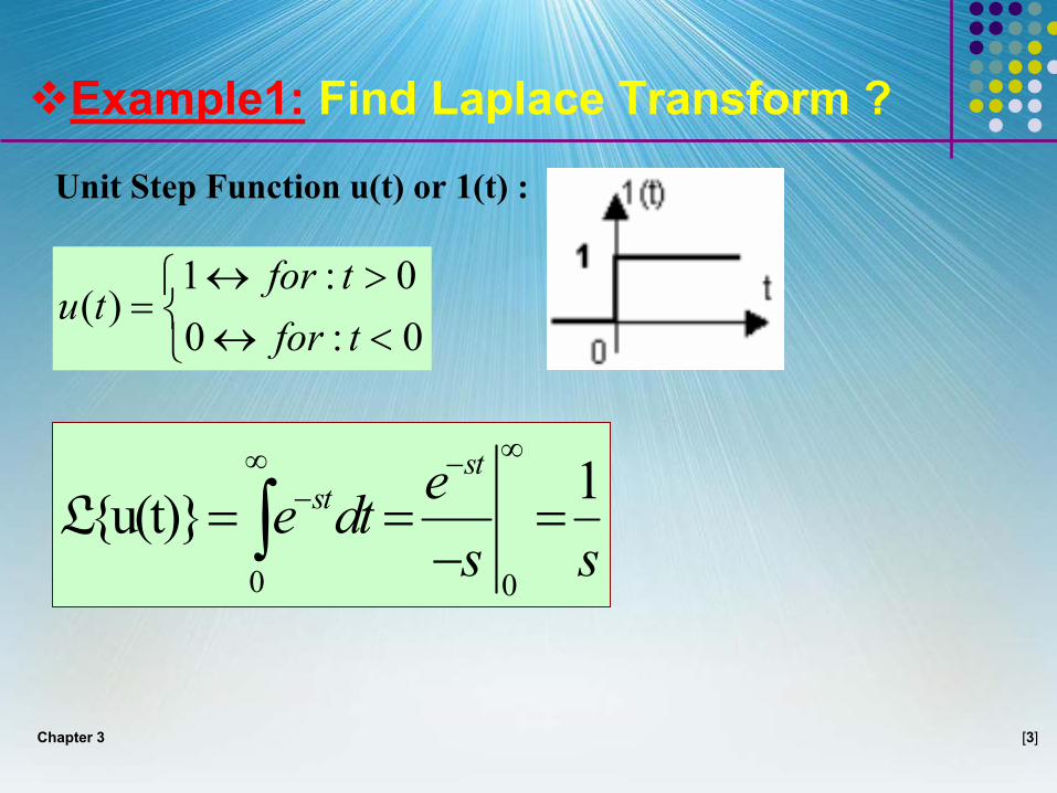
Example1: Find Laplace Transform ?

0 0

1{u(t)}∞∞ −

−= = =−∫st

st ee dts s

L

1 : 0( )

0 : 0↔ >

= ↔ <

for tu t

for t

Unit Step Function u(t) or 1(t) :

Chapter 3 [4]

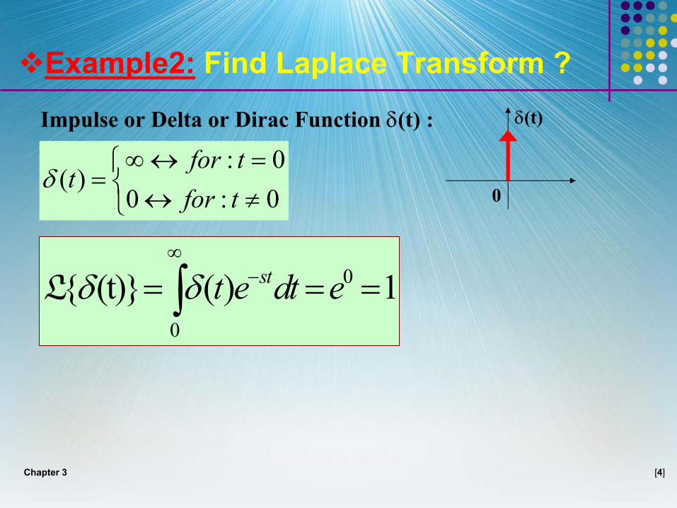
Example2: Find Laplace Transform ?

0

0

{ (t)} ( ) 1∞

−= = =∫ stt e dt eδ δL

: 0( )

0 : 0∞↔ =

= ↔ ≠

for tt

for tδ

Impulse or Delta or Dirac Function δ(t) : δ(t)

0

Chapter 3 [5]

3.2: Properties of Laplace Transform :

1) Multiplication by a constant :

{f(t)} F(s)=LIf:

{k.f(t)} k.F(s)=LThen:

Chapter 3 [6]

2) Addition / Subtraction:

1 1 2 2{f (t)} F (s) and {f (t)} F (s)= =L LIf:

1 2 1 2{f (t) f (t) } F (s) F (s)± = ±LThen:

Chapter 3 [7]

3) Translation in Time-domain:

0st0 0{f(t t ).u(t t ) } F(s).e−− − =LThen:

{f(t)} F(s)=LIf:

Chapter 3 [8]

4) Translation in frequency-domain:

at{f(t).e } F(s a)− = +LThen:

{f(t)} F(s)=LIf:

Chapter 3 [9]

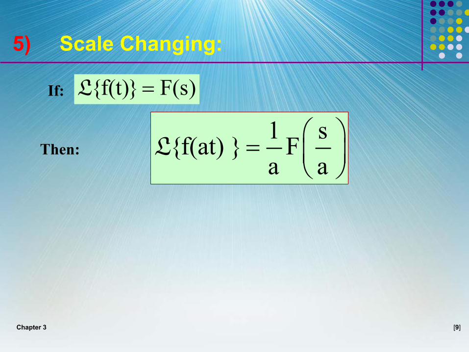
5) Scale Changing:

1 s{f(at) } Fa a

=

LThen:

{f(t)} F(s)=LIf:

Chapter 3 [10]

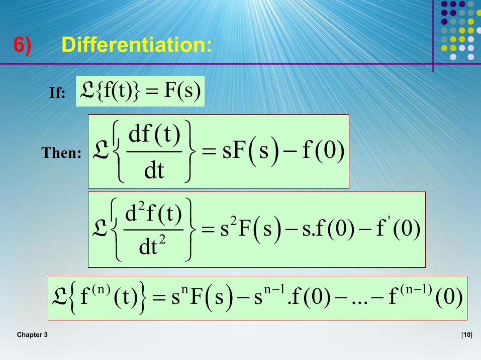
6) Differentiation:

( )df (t) sF s f (0)dt

= − LThen:

{f(t)} F(s)=LIf:

( )2

2 '2

d f (t) s F s s.f (0) f (0)dt

= − −

L

{ } ( )(n) n n 1 (n 1)f (t) s F s s .f (0) ... f (0)− −= − − −L

Chapter 3 [11]

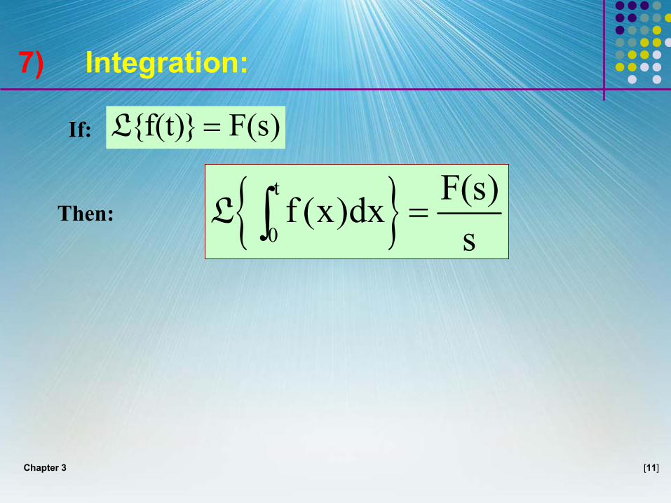
7) Integration:

{ }t

0

F(s)f (x)dxs

=∫LThen:

{f(t)} F(s)=LIf:

Chapter 3 [12]

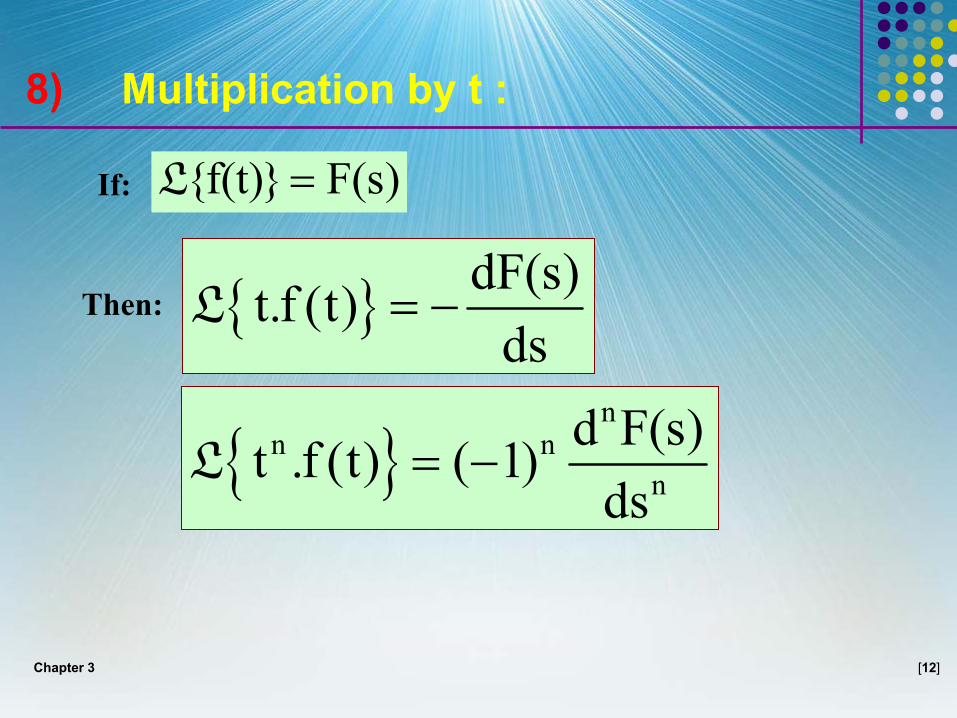
8) Multiplication by t :

{ } dF(s)t.f (t)ds

= −LThen:

{f(t)} F(s)=LIf:

{ }n

n nn

d F(s)t .f (t) ( 1)ds

= −L

Chapter 3 [13]

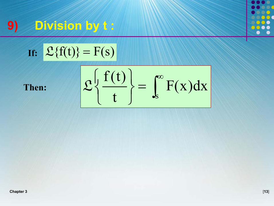
9) Division by t :

s

f (t) F(x)dxt

∞ = ∫LThen:

{f(t)} F(s)=LIf:

Chapter 3 [14]

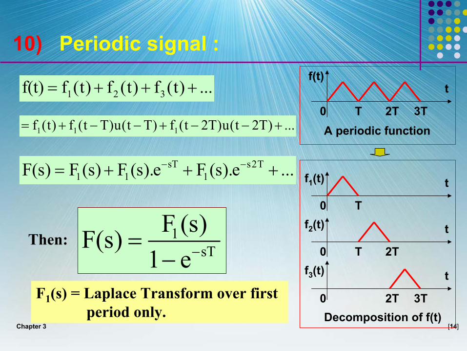
10) Periodic signal :

1 2 3f(t) f (t) f (t) f (t) ...= + + +f(t)

t

A periodic function0 T 2T 3T

f1(t) t

0 Tf2(t) t

0 T 2Tf3(t) t

0 2T 3TDecomposition of f(t)

1 1 1f (t) f (t T)u(t T) f (t 2T)u(t 2T) ...= + − − + − − +

sT s2T1 1 1F(s) F (s) F (s).e F (s).e ...− −= + + +

Then: 1sT

F (s)F(s)1 e−=−

F1(s) = Laplace Transform over firstperiod only.

Chapter 3 [15]

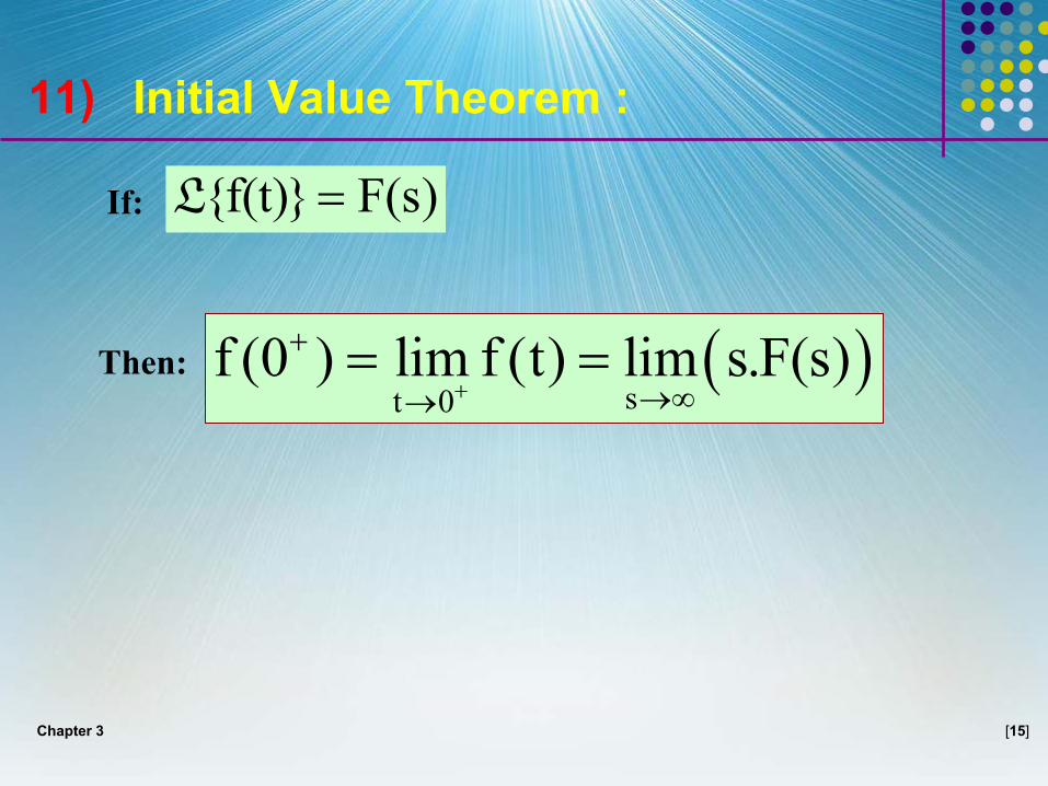
11) Initial Value Theorem :

( )st 0

f (0 ) lim f (t) lim s.F(s)+

+

→∞→= =Then:

{f(t)} F(s)=LIf:

Chapter 3 [16]

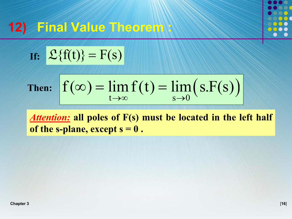
12) Final Value Theorem :

( )t s 0

f ( ) lim f (t) lim s.F(s)→∞ →

∞ = =Then:

{f(t)} F(s)=LIf:

Attention: all poles of F(s) must be located in the left half of the s-plane, except s = 0 .

Chapter 3 [17]

3.3: Laplace Transform of Fundamental functions :

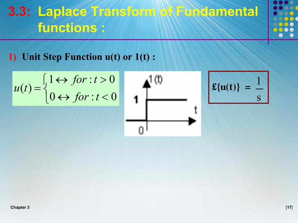
1 : 0( )

0 : 0↔ >

= ↔ <

for tu t

for t

1) Unit Step Function u(t) or 1(t) :

£{u(t)} = 1s

Chapter 3 [18]

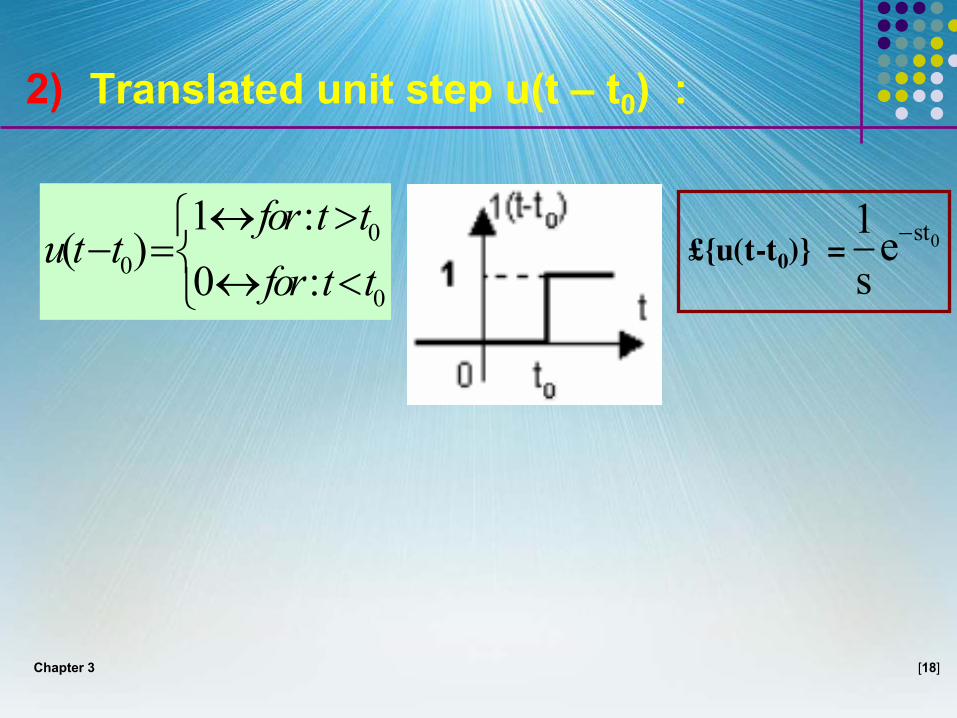
2) Translated unit step u(t – t0) :

00

0

1 :( )

0 :↔ >

− = ↔ <

for t tu t t

for t t£{u(t-t0)} = 0st1e

s−

Chapter 3 [19]

3) Impulse or Delta Function δ(t) :

£{δ(t)} = 10 : 0

( ) '( ): 0

↔ ≠= = ∞↔ =

for tt u t

for tδ

Chapter 3 [20]

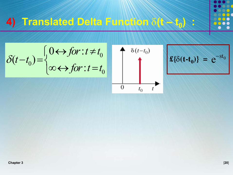
4) Translated Delta Function δ(t – t0) :

£{δ(t-t0)} = 0ste−00

0

0 :( )

:↔ ≠

− =∞↔ =

for t tt t

for t tδ

Chapter 3 [21]

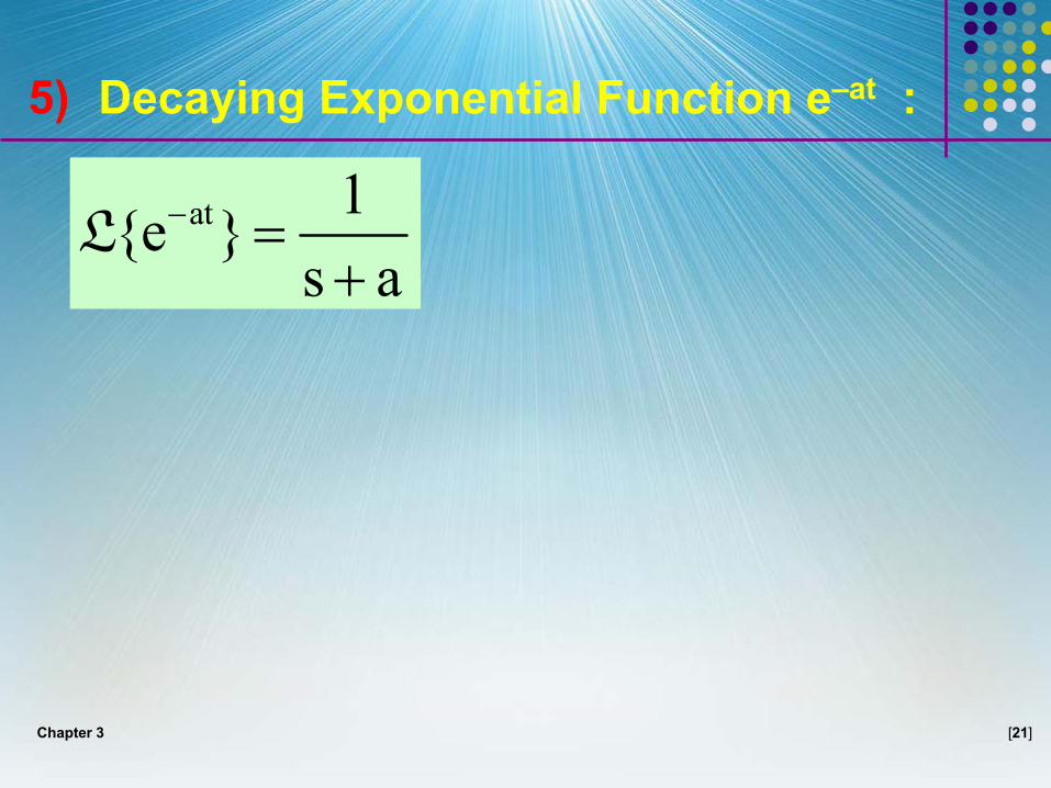
5) Decaying Exponential Function e–at :

at 1{e }s a

− =+

L

Chapter 3 [22]

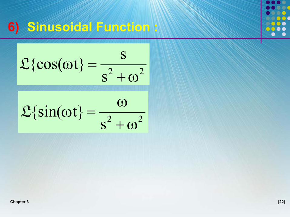
6) Sinusoidal Function :

2 2

s{cos( t}s

ω =+ω

L

2 2{sin( t}sω

ω =+ω

L

Chapter 3 [23]

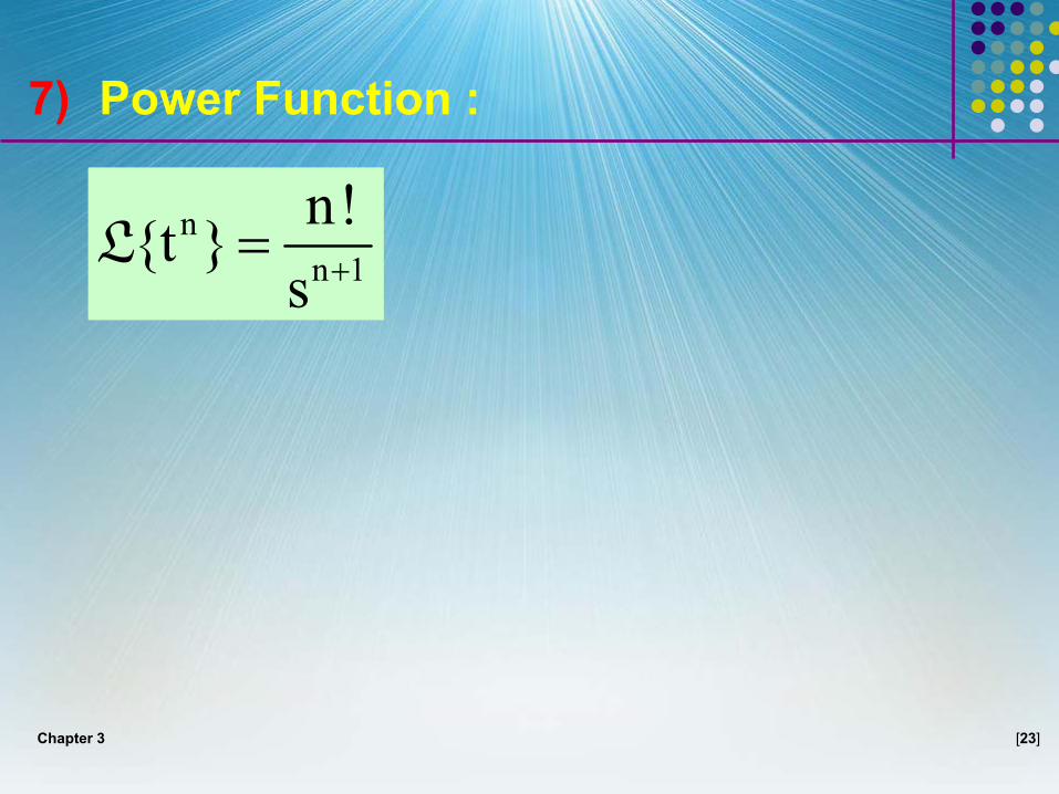
7) Power Function :

nn 1

n!{t }s +=L

Chapter 3 [24]

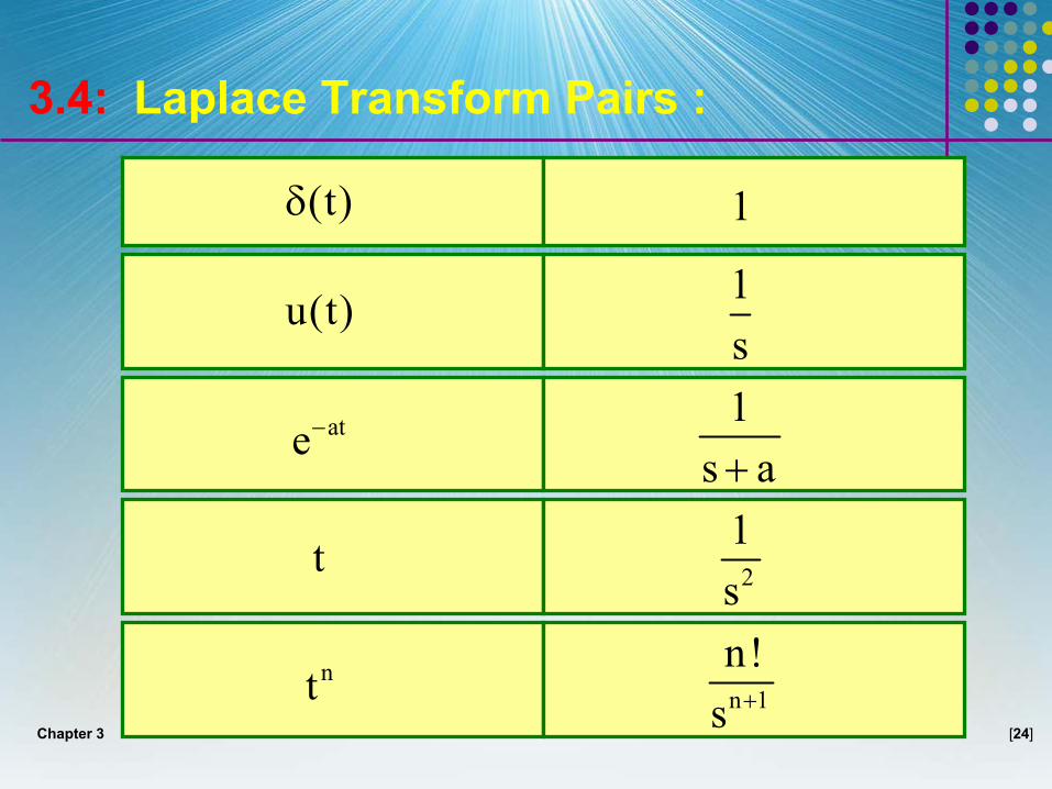
3.4: Laplace Transform Pairs :

(t)δ 1

u(t) 1s

ate− 1s a+

t 2

1s

nt n 1

n!s +

Chapter 3 [25]

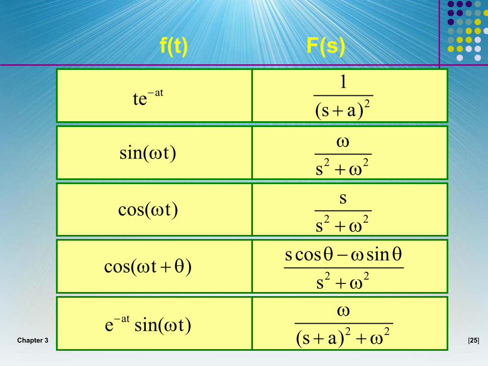
f(t) F(s)

atte−2

1(s a)+

sin( t)ω 2 2sω+ω

cos( t)ω 2 2

ss +ω

cos( t )ω +θ 2 2

s cos sinsθ−ω θ+ω

ate sin( t)− ω 2 2(s a)ω

+ +ω

Chapter 3 [26]

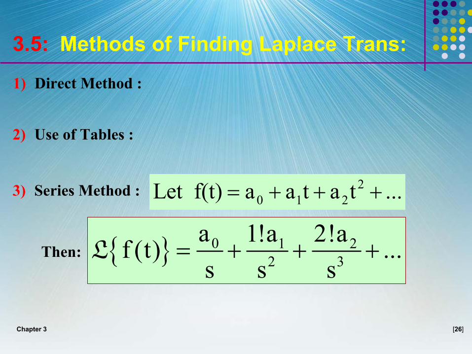
3.5: Methods of Finding Laplace Trans:

1) Direct Method :

3) Series Method :

{ } 0 1 22 3

a 1!a 2!af (t) ...s s s

= + + +LThen:

20 1 2Let f(t) a a t a t ...= + + +

2) Use of Tables :

Chapter 3 [27]

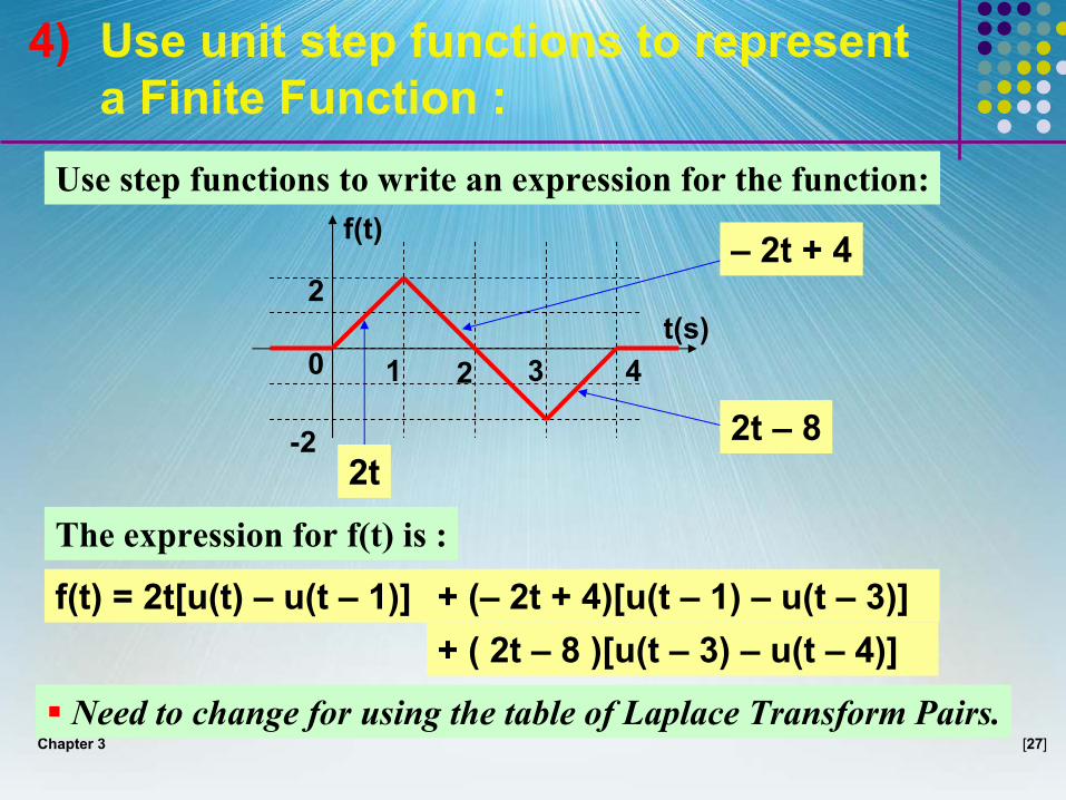
4) Use unit step functions to represent a Finite Function :

Use step functions to write an expression for the function:f(t)

0

2

-2

1 2 3 4t(s)

2t

– 2t + 4

2t – 8

The expression for f(t) is :

f(t) = 2t[u(t) – u(t – 1)] + (– 2t + 4)[u(t – 1) – u(t – 3)] + ( 2t – 8 )[u(t – 3) – u(t – 4)]

Need to change for using the table of Laplace Transform Pairs.

Chapter 3 [28]

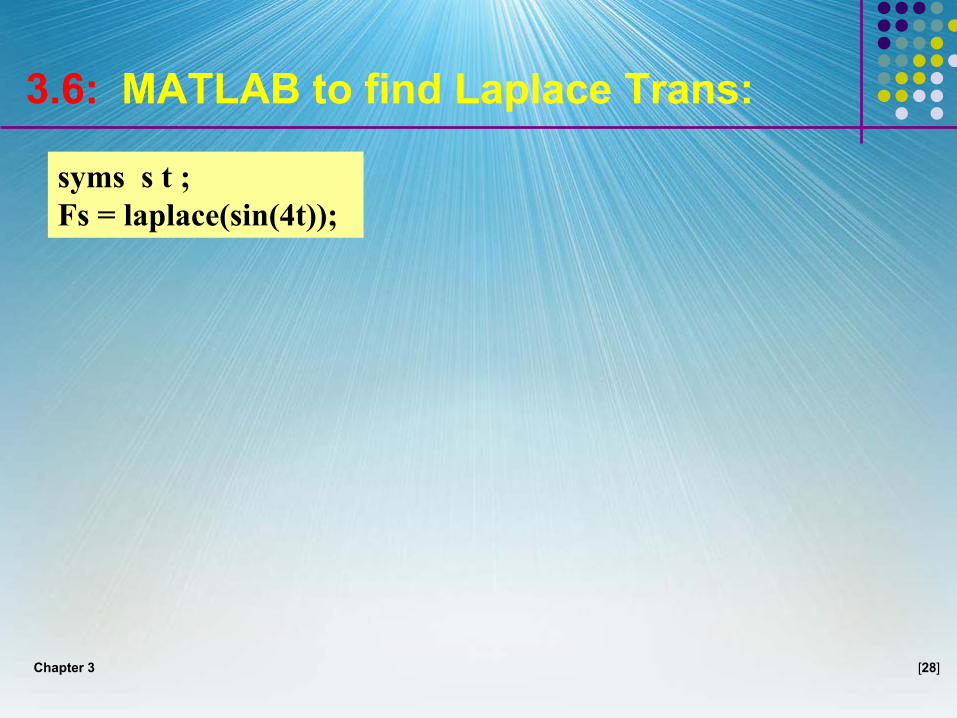
3.6: MATLAB to find Laplace Trans:

syms s t ; Fs = laplace(sin(4t));