Control-flow Refinement and Progress Invariantsfor Bound Analysis

Sumit Gulwani

Microsoft Research, Redmond

sumitg@microsoft.com

Sagar Jain

IIT Kanpur

sagarj@iitk.ac.in

Eric Koskinen

University of Cambridge

ejk39@cam.ac.uk

Abstract

Symbolic complexity bounds help programmers understand theperformance characteristics of their implementations. Existingwork provides techniques for statically determining bounds of pro-cedures with simple control-flow. However, procedures with nestedloops or multiple paths through a single loop are challenging.

In this paper we describe two techniques, control-flow refine-ment and progress invariants, that together enable estimation ofprecise bounds for procedures with nested and multi-path loops.Control-flow refinement transforms a multi-path loop into a seman-tically equivalent code fragment with simpler loops by making thestructure of path interleaving explicit. We show that this enablesnon-disjunctive invariant generation tools to find a bound on manyprocedures for which previous techniques were unable to provetermination. Progress invariants characterize relationships betweenconsecutive states that can arise at a program location. We furtherpresent an algorithm that uses progress invariants to compute pre-cise bounds for nested loops. The utility of these two techniquesgoes beyond our application to symbolic bound analysis. In partic-ular, we discuss applications of control-flow refinement to provingsafety properties that otherwise require disjunctive invariants.

We have applied our methodology to over 670,000 lines of codeof a significant Microsoft product and were able to find symbolicbounds for 90% of the loops. We are not aware of any otherpublished results that report experiences running a bound analysison a real code-base.

Categories and Subject Descriptors C.4 [Performance of Sys-tems]: Measurement techniques; Reliability, availability, and ser-viceability; D.2.4 [Software Engineering]: Software/Program Ver-ification; D.4.5 [Operating Systems]: Reliability—Verification;D.4.8 [Operating Systems]: Performance—Modeling and pre-diction; F.3.1 [Logics and Meanings of Programs]: Specifyingand Verifying and Reasoning about Programs; F.3.2 [Logics andMeanings of Programs]: Semantics of Programming Languages—Program analysis

General Terms Verification, Performance, Reliability

Keywords Bound analysis, Termination, Control-flow refinement,Progress invariants, Program verification, Formal verification

Permission to make digital or hard copies of all or part of this work for personal orclassroom use is granted without fee provided that copies are not made or distributedfor profit or commercial advantage and that copies bear this notice and the full citationon the first page. To copy otherwise, to republish, to post on servers or to redistributeto lists, requires prior specific permission and/or a fee.

PLDI’09, June 15–20, 2009, Dublin, Ireland.Copyright c© 2009 ACM 978-1-60558-392-1/09/06. . . $5.00

1. Introduction

Software engineers lack the tools they need to build robust, efficientsoftware. They are therefore forced to rely on existing techniquessuch as testing and performance profiling which are limited, leavingmany usage scenarios uncovered. In particular, as processor clockspeeds begin to plateau, there is an increasing need to focus onsoftware performance.

This paper addresses the problem of statically generating sym-bolic complexity bounds for procedures in a program, given a costmodel for atomic program statements. Automated methods of gen-erating symbolic complexity bounds offer a significant advance inaiding the performance aspects of the software life cycle. Thoughprogrammers are often cognizant of the intended complexity of analgorithm, concrete implementations can differ. Moreover, sym-bolic bounds can highlight the impact of changes and illuminateperformance of unfamiliar APIs.

The most challenging aspect of computing complexity boundsis calculating a bound on the number of iterations of a given loop.Two kinds of techniques have been proposed for automaticallybounding loop iterations: pattern matching [18] and counter in-strumentation [17, 12, 15]. Unfortunately, these techniques havelimitations: (i) They compute bounds for simple loops that havea single path (a straight-line sequence of statements) or a set ofpaths with similar effect, but not multi-path loops that have multi-ple paths with different effects and non-trivial interleaving patterns.(ii) They compute conservative bounds in presence of nested loopssince they simply compose bounds for individual loops based onstructural decomposition of the program. In this paper, we presenttechniques that address these limitations.

The first technical contribution of our work is a novel techniquecalled control-flow refinement, which is a semantics- and bound-preserving transformation on procedures. Specifically, a loop thatconsists of multiple paths (arising from conditionals) is trans-formed into a code fragment with one or more loops in which theinterleaving of paths is syntactically explicit. We describe an algo-rithm (Section 4) that explores all path interleavings in a recursivefashion using an underlying invariant generation tool. The proce-dure with transformed loop enables a more precise analysis (e.g.with the same invariant generation tool) than would have been pos-sible with the original loop. The additional program points createdby refinement allow the invariant generator to store more informa-tion about the procedure. Different invariants at related programpoints in the refined loop correspond to a disjunctive invariant atthe original location in the original loop. We detail the applicationof the control-flow refinement technique for symbolic bound anal-ysis (Section 4.3). The technique enables bound computation forloops for which no other technique can even establish termination(Section 2.1).

(a) Original Procedure (b) Change of notation (c) Expanded Loop (d) Final Refined Loop

cyclic(int id, maxId):assume(0 ≤ id < maxId);int tmp := id+1;while(tmp 6=id && nondet)

if (tmp ≤ maxId)tmp := tmp + 1;

elsetmp := 0;

cyclic(int id, maxId):assume(0≤id<maxId);int tmp := id+1;Repeat(Choose({ρ1,ρ2}));

cyclicref(int id, maxId):1 assume(0≤id<maxId);2 int tmp := id+1;3 Choose({4 skip,

5 Repeat+(ρ1),

6 Repeat+(ρ2),

7 Repeat+(ρ1);ρ2;Repeat(Choose({ρ1,ρ2})),

8 Repeat+(ρ2);ρ1;Repeat(Choose({ρ1,ρ2}))9 });

cyclicpruned(int id, maxId):10 assume(0 ≤ id < maxId);11 int tmp := id+1;12 Choose({13 skip,

14 Repeat+(ρ1);ρ2;Repeat(ρ1),

15 Repeat+(ρ1)16 });

ρ1 , assume(tmp6=id ∧ tmp≤maxId); tmp:=tmp+1; ρ2 , assume(tmp6=id ∧ tmp>maxId); tmp:=0;

Figure 1: (a) illustrates an iteration pattern seen in product code. (b),(c), and (d) show control-flow refinement of the multi-path loop in (a).

The second technical contribution of our work is the notion ofprogress invariants that describe relationships between any twoconsecutive states that can arise at a given program location. Wepresent an algorithm for computing such relationships using a stan-dard invariant generator (Section 5). The algorithm runs the invari-ant generation tool over a procedure appropriately modified andinstrumented with extra variables that copy the program state at ap-propriate locations. We observe that progress invariants are moreprecise than the related notion of transition invariants [24] or vari-ance analyses [5] (recently described in literature for proving ter-mination), which describe relationships between a state at a pro-gram location and any other previous state at that location. Tran-sition invariants can be generated from progress invariants but notvice-versa. (See discussion in Section 9). We believe the notion ofprogress invariants to have applications beyond bound analysis.

A further contribution is that we show (in Section 6) how to useprogress invariants to compute a precise bound for nested loops.This technique applies to procedures that may have been control-flow refined. The key idea is to use progress invariants to illuminaterelationships between any two consecutive states of an inner loopper iteration of some dominating outer loop (as opposed to theimmediately dominating outer loop). This information is then usedto compute the amortized complexity of an inner loop. Such anamortized complexity yields a more precise bound when nestedloops share same iterators, which occurs often in practice.

In summary, we make the following contributions:

1. We introduce control-flow refinement, a novel program trans-formation that allows standard invariant generators to reasonabout loops with structured interleaving between paths in theloop body. This transformation has applications beyond boundanalysis, and briefly discuss one such application on provingnon-trivial safety properties of procedures that otherwise re-quire specialized analyses [13, 19, 14, 10, 17] (Section 8).

2. We define progress invariants, which describe relationships be-tween a state at a program location and the previous state atthe same location, and show how to compute them. Progress in-variants have applications beyond bound analysis. For examplethey can be applied to the problem of fair termination (provingprocedure termination under fairness constraints).

3. We define an algorithm for computing precise bounds of nestedloops using progress invariants (Section 6).

4. To the best of our knowledge, we present the first experimentalresults for bound analysis on the source of a significant Mi-crosoft product (Section 7). We have built a full interproce-dural bound analysis for C++, using C# and F# on top of thePhoenix [1] compiler. Our results show that 90% of non-trivialprocedures can be bounded with our technique (Section 7.2).

2. Overview

In this section we illustrate the challenges offered by multi-pathloops and nested loops in computing precise bounds for procedures.We also briefly describe our two key techniques that address thesechallenges; these techniques are described in more detail in thesubsequent sections. The examples are adapted from the source ofa large Microsoft product. For clarity, we have distilled their corecontrol flow and renamed some variables.

2.1 Multi-Path Loops

Consider the example in Figure 1(a), which is adapted from theproduct code. This procedure is a form of “cyclic” iteration: ini-tially tmp is equal to id+1, tmp is incremented until it reachesmaxId+1 (along the tmp ≤ maxId branch), tmp is then reset to0 (along the else branch), and finally tmp is incremented until itreaches id. We would like to automatically conclude that the totalnumber of iterations for this loop is bounded above by maxId+1.

None of the bound analysis techniques that we know of canautomatically compute a bound for such a loop. This is becausepath-sensitive disjunctive invariants are required to establish abound. Recent work [15] proposes elaborate counter instrumen-tation strategies to reduce dependence on disjunctive invariants, yetwould fail to compute a bound because the invariants required arepath-sensitive. In fact, we do not know of any technique that caneven prove termination of this procedure. Recent techniques [6, 5]based on disjunctively well-founded ranking functions [24] failfor this example because there does not exist a disjunctively well-founded linear ranking function.

The mildly complex control flow in the loop foils all knownapproaches. A detailed analysis of the failure of these approacheson this example would illustrate that these approaches tend to con-sider all possible interleavings between the two paths through theloop. However, the two paths are interleaved in a more structuredmanner. Let us represent the control-flow using a regular expres-sion, letting ρ1 and ρ2 denote the increment and reset branches,respectively. Then, the path interleavings in the example loop canbe more precisely described by the refinement (ρ∗

1ρ2ρ∗

1)|(ρ∗

1) ofthe original control-flow (ρ1|ρ2)

∗. While (ρ1|ρ2)∗ suggests that

paths ρ1 and ρ2 can interleave in an arbitrary manner, the refine-ment (ρ∗

1ρ2ρ∗

1)|(ρ∗

1) explicitly indicates that path ρ2 executes atmost once. Next, we briefly describe how such a refinement can becarried out automatically, and how it enables bound computation.

Control-flow Refinement The first key idea of this paper is atechnique called control-flow refinement. Rather than abstractingthe control-flow, which blurs interleavings, we instead refine thecontrol-flow by making interleavings more explicit. Subsequently,an invariant generation tool may determine that some paths areinfeasible, often resulting in a procedure that is easier to analyze.

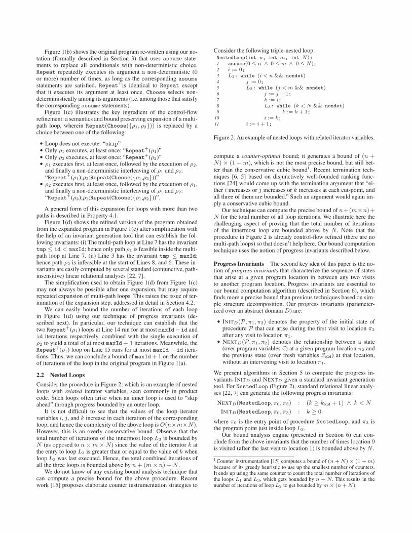
Figure 1(b) shows the original program re-written using our no-tation (formally described in Section 3) that uses assume state-ments to replace all conditionals with non-deterministic choice.Repeat repeatedly executes its argument a non-deterministic (0or more) number of times, as long as the corresponding assumestatements are satisfied. Repeat+is identical to Repeat exceptthat it executes its argument at least once. Choose selects non-deterministically among its arguments (i.e. among those that satisfythe corresponding assume statements).

Figure 1(c) illustrates the key ingredient of the control-flowrefinement: a semantics and bound preserving expansion of a multi-path loop, wherein Repeat(Choose({ρ1, ρ2})) is replaced by achoice between one of the following:

• Loop does not execute: “skip”• Only ρ1 executes, at least once: “Repeat+(ρ1)”• Only ρ2 executes, at least once: “Repeat+(ρ2)”• ρ1 executes first, at least once, followed by the execution of ρ2,

and finally a non-deterministic interleaving of ρ1 and ρ2:“Repeat+(ρ1);ρ2;Repeat(Choose({ρ1,ρ2}))”

• ρ2 executes first, at least once, followed by the execution of ρ1,and finally a non-deterministic interleaving of ρ1 and ρ2:“Repeat+(ρ2);ρ1;Repeat(Choose({ρ1,ρ2}))”.

A general form of this expansion for loops with more than twopaths is described in Property 4.1.

Figure 1(d) shows the refined version of the program obtainedfrom the expanded program in Figure 1(c) after simplification withthe help of an invariant generation tool that can establish the fol-lowing invariants: (i) The multi-path loop at Line 7 has the invarianttmp ≤ id < maxId; hence only path ρ1 is feasible inside the multi-path loop at Line 7. (ii) Line 3 has the invariant tmp ≤ maxId;hence path ρ2 is infeasible at the start of Lines 8, and 6. These in-variants are easily computed by several standard (conjunctive, path-insensitive) linear relational analyses [22, 7].

The simplification used to obtain Figure 1(d) from Figure 1(c)may not always be possible after one expansion, but may requirerepeated expansion of multi-path loops. This raises the issue of ter-mination of the expansion step, addressed in detail in Section 4.2.

We can easily bound the number of iterations of each loopin Figure 1(d) using our technique of progress invariants (de-scribed next). In particular, our technique can establish that thetwo Repeat+(ρ1) loops at Line 14 run for at most maxId− id andid iterations respectively, combined with the single execution ofρ2 to yield a total of at most maxId + 1 iterations. Meanwhile, theRepeat+(ρ1) loop on Line 15 runs for at most maxId − id itera-tions. Thus, we can conclude a bound of maxId+ 1 on the numberof iterations of the loop in the original program in Figure 1(a).

2.2 Nested Loops

Consider the procedure in Figure 2, which is an example of nestedloops with related iterator variables, seen commonly in productcode. Such loops often arise when an inner loop is used to “skipahead” through progress bounded by an outer loop.

It is not difficult to see that the values of the loop iteratorvariables i, j, and k increase in each iteration of the correspondingloop, and hence the complexity of the above loop is O(n×m×N).However, this is an overly conservative bound. Observe that thetotal number of iterations of the innermost loop L3 is bounded byN (as opposed to n × m × N ) since the value of the iterator k atthe entry to loop L3 is greater than or equal to the value of k whenloop L3 was last executed. Hence, the total combined iterations ofall the three loops is bounded above by n + (m × n) + N .

We do not know of any existing bound analysis technique thatcan compute a precise bound for the above procedure. Recentwork [15] proposes elaborate counter instrumentation strategies to

Consider the following triple-nested loop.NestedLoop(int n, int m, int N):1 assume(0 ≤ n ∧ 0 ≤ m ∧ 0 ≤ N);2 i := 0;3 L1: while (i < n && nondet)4 j := 0;5 L2: while (j < m && nondet)6 j := j + 1;7 k := i;8 L3: while (k < N && nondet)9 k := k + 1;

10 i := k;11 i := i + 1;

Figure 2: An example of nested loops with related iterator variables.

compute a counter-optimal bound; it generates a bound of (n +N) × (1 + m), which is not the most precise bound, but still bet-

ter than the conservative cubic bound1. Recent termination tech-niques [6, 5] based on disjunctively well-founded ranking func-tions [24] would come up with the termination argument that “ei-ther i increases or j increases or k increases at each cut-point, andall three of them are bounded.” Such an argument would again im-ply a conservative cubic bound.

Our technique can compute the precise bound of n+(m×n)+N for the total number of all loop iterations. We illustrate here thechallenging aspect of proving that the total number of iterationsof the innermost loop are bounded above by N . Note that theprocedure in Figure 2 is already control-flow refined (there are nomulti-path loops) so that doesn’t help here. Our bound computationtechnique uses the notion of progress invariants described below.

Progress Invariants The second key idea of this paper is the no-tion of progress invariants that characterize the sequence of statesthat arise at a given program location in between any two visitsto another program location. Progress invariants are essential toour bound computation algorithm (described in Section 6), whichfinds more a precise bound than previous techniques based on sim-ple structure decomposition. Our progress invariants (parameter-ized over an abstract domain D) are:

• INITD(P, π1, π2) denotes the property of the initial state ofprocedure P that can arise during the first visit to location π2

after any visit to location π1.• NEXTD(P, π1, π2) denotes the relationship between a state

(over program variables ~x) at a given program location π2 andthe previous state (over fresh variables ~xold) at that location,without an intervening visit to location π1.

We present algorithms in Section 5 to compute the progress in-variants INITD and NEXTD given a standard invariant generationtool. For NestedLoop (Figure 2), standard relational linear analy-ses [22, 7] can generate the following progress invariants:

NEXTD(NestedLoop, π0, π3) : (k ≥ kold + 1) ∧ k < N

INITD(NestedLoop, π0, π3) : k ≥ 0

where π0 is the entry point of procedure NestedLoop, and π3 isthe program point just inside loop L3.

Our bound analysis engine (presented in Section 6) can con-clude from the above invariants that the number of times location 9is visited (after the last visit to location 1) is bounded above by N .

1 Counter instrumentation [15] computes a bound of (n + N) × (1 + m)because of its greedy heuristic to use up the smallest number of counters.It ends up using the same counter to count the total number of iterations ofthe loops L1 and L3, which gets bounded by n + N . This results in thenumber of iterations of loop L2 to get bounded by m × (n + N).

3. Notation

We now turn to a formal model of our techniques. In this section,we introduce some notation which we will use in the subsequentsections when we present path refinement and our precise methodof calculating procedure bounds.

3.1 Program Model

For simplicity of presentation, we assume that each procedure P isdescribed as a statement s using the following structural language:

s ::= s1; s2 | Repeat(s) | Choose({s1, . . , st})

| x := e | assume(cond) | skip

where x is a variable from the set of all variables ~x, e is someexpression, and cond is some boolean expression. The expressione can contain procedure calls2.

The above model has the following intuitive semantics. Sincethere are non-deterministic conditionals, its semantics can be char-acterized by showing its operational semantics on a set of states.The following function JsKσ illustrates how a statement s trans-forms a set σ of concrete states.

JskipKσ = σ

Js1; s2Kσ = Js2K(Js1Kσ)

JChoose({s1, . . , st})Kσ = Js1Kσ ∪ . . ∪ JstKσ

JRepeat(s)Kσ = σ ∪ Js; Repeat(s)Kσ

Jx := eKσ = {δ[x 7→ δ(e)] | δ ∈ σ}

Jassume(cond)Kσ = {δ | δ ∈ σ, δ(cond) = true}

where δ(e) and δ(cond) respectively denote the value of expres-sion e or cond in state δ. We often use the notation Repeat+(s)to denote “s; Repeat(s).” Standard deterministic control flow inbranches and loops can be modeled in our notation as follows.

if(c)s1 else s2 Choose({(assume(c); s1), (assume(¬c); s2)})

while(c)s1 Repeat(assume(c); s1); assume(¬c);

3.2 Abstract Domain

Our framework is parameterized by a standard abstract domain D,with an abstract element denoted E. However operations in the ab-stract domain only occur behind the curtains of the invariant gen-erator INVARIANTD . The only abstract element which appears ex-plicitly in our algorithms is the minimal element ⊥D . Our tech-niques are inter-operable with a variety of existing tools, so we willuse some APIs throughout the paper. We assume an invariant gen-erator INVARIANTD(P, π, SD(~x)) → SR

D(~x, ~x′) which takes aprocedure P , a program point π, an abstract state SD over programvariables ~x, and returns an invariant SR

D which holds at π. Thisinvariant generator can be for any abstract domain D.

4. Control-flow Refinement

In this section, we present a technique called control-flow refine-ment, which is a semantics-preserving and bound-preserving trans-formation of loops within a procedure. Specifically, a loop consist-ing of multiple paths (resulting from a conditional) is refined intoone or more loops in which the interleaving of paths is syntacticallyexplicit. Subsequently, an invariant generation tool may determinethat some paths are infeasible, often resulting in an overall proce-dure that is easier to analyze.

Our algorithm is described in Section 4.2. It uses an operationcalled FLATTEN that we introduce next.

2 Procedure calls may have side effects, but for simplicity we define thesemantics of Jx := eKσ assuming the absence of side effects.

REFINE(P:Procedure, sloop:Repeat statement)1 let sloop be Repeat(s) occurring at location π in P.2 E := INVARIANTD(P, π, true);3 s := FLATTEN(s);4 Q := Push(E, Empty Stack);5 (sresult, Z) := R(s, Q);6 return P with sloop replaced by sresult;

R(s:Flattened stmt, Q:stack of abstract elements)1 let s be of the form Choose({ρ1, . . , ρt}).2 E := Top(Q);3 for i = 1 to t

4 si := (Repeat+(ρi); Choose({ρ1, . . , ρi−1, ρi+1, ρt}));5 πex := exit point of si;6 E′ := INVARIANTD(si, πex, E);7 if (E′ = ⊥D) si := ⊥;8 else if (∃Et ∈ Q s.t.E′ = Et) Zi := {E′};9 else (s′, Zi) := R(s, Push(Q, E′)); si := si; s

′;10 Sif := {skip}; Swh := ∅;11 for i = 1 to t

12 Sif := Sif ∪ {Repeat+(ρi)};13 if (si = ⊥) continue;14 if (∃Et ∈ Zi s.t.Et = E) Swh := Swh ∪ {si};15 else Sif := Sif ∪ {si};16 Z := Z ∪ Zi − {E};17 return (Choose(Sif ∪ Repeat(Choose(Swh))), Z);

Figure 3: The algorithm REFINE for refining the control-flow of a

loop Repeat(s) in initial state E by invoking REFINE(s, E).

4.1 Flattening of a statement

Definition 4.1 (Flatten). Given a statement s, we define FLATTEN(s)to be a statement of the form Choose({ρ1, . . , ρt}) such that forany set of states σ, we have:

JsKσ = JChoose({ρ1, . . , ρt})Kσ

where each ρi is a straight line sequence of atomic x := e orassume statements or Repeat loops (and, importantly, no Choose

statements). We refer to such ρi as a path.

The flatten operation can be implemented as:

FLATTEN(s) = Choose(F(s))

where the function F(s) maps a statement s into a set of straight-line sequences as follows:

F(s1; s2) = {ρ1; ρ2 | ρ1 ∈ F(s1), ρ2 ∈ F(s2)}

F(Choose({s1, . . , st})) = F(s1) ∪ . . ∪ F(st)

F(s) = {s} for all other s

Example 1. Consider the following code fragment.

sdef= if c then s1 else s11; s2; if c

′then s3;

Flattening of the above code fragment yields, in our notation:Choose({ assume(c); s1; s2; assume(c′); s3,

assume(¬c); s11; s2; assume(c′); s3,assume(c); s1; s2; assume(¬c′),assume(¬c); s11; s2; assume(¬c′) })

4.2 Refinement of a loop

The REFINE algorithm in Figure 3 performs control-flow refine-ment of a multi-path loop sloop in the initial state E, and returns aprocedure that is semantically equivalent in the input state E (The-orem 4.1). The key idea is to use the following property that de-scribes how a flattened, multi-path loop can be unfolded into 2t+1different cases depending on which loop path iterates first, andwhether any other path iterates afterwards. This is the generaliza-tion of the two-path loop discussed in Section 2.1.

Property 4.1. Let s and si (for 1 ≤ i ≤ t) be as follows.

sdef= Choose({ρ1, . . , ρt})

sidef= Repeat+(ρi); Choose({ρ1, . . , ρi−1, ρi+1, . . , ρt}); Repeat(s)

s′idef= Repeat+(ρi);

Then, for any set of states σ, we have:

JRepeat(s)Kσ = JChoose({skip, s1, . . , st, s′

1, . . , s′

t})Kσ

Of these 2t + 1 cases, there are t cases (corresponding tos1, . . , st) that have multi-path loops, which are then further refinedrecursively. To ensure termination, we use an underlying invariantgenerator INVARIANTD to compute the state before each newlycreated multi-path loop. We then either stop the recursive explo-ration (if INVARIANTD can establish unreachability), put a back-edge (if INVARIANTD finds a state already seen), or use wideningheuristics (in case INVARIANTD generates invariants over an infi-nite domain). Note that although our algorithm is exponential inthe number of paths through the body of the loop, we use a strictslicing technique to keep the constants small. Our slicing technique(described in Section 7.1) reduces the number of paths by collaps-ing branches that do not impact the iterations of the loop into asingle path.

The REFINE algorithm invokes a recursive algorithm R on theflattened body s of the input loop, along with a stack containingthe element E, which is the only input configuration seen beforeany loop. R consumes a flattened loop body s and a stack Q ofabstract elements. Q represent the input abstract states immediatelybefore the while loop Repeat(s) seen during the earlier (but yetunfinished) recursive calls to R. R returns a pair (s′′, Z) where s′′

is a statement and Z is a set of input abstract states that were re-visited by the recursive algorithm during the refinement and usedto terminate exploration at the promise of arranging a nested loopat appropriate places.

The first loop in R (Lines 3-9) recursively refines the t cases(s1, . . , st) from Property 4.1 that have multi-path loops, one byone. R refines si by choosing between one of the following 3possibilities depending on the element E′ computed before themulti-path loop in si:

• Stop exploration (Line 7) if E′ = ⊥D , denoting unreachability.• Create a nested loop (Line 8) if E′ belongs to stack Q (i.e. it is

an input state that has been seen before). Further exploration isstopped and E′ is returned to denote the place where the nestedloop needs to be created.

• Pursue more exploration (Line 9) otherwise, recursively.

If the abstract domain D is a finite domain, then the first loopin R terminates because the algorithm is never recursively invokedwith the same input state E twice. Otherwise additional measuresare required to ensure termination. A trivial way to ensure termi-nation this would be to override the equality check in Line 8 withreturn true if the size of stack Qi becomes equal to some prese-lected constant. A better way to accomplish this is with a wideningalgorithm associated with the domain D, wherein the contents ofthe stack Qi are treated as that of the corresponding widening se-quence for purpose of checking equality.

The second loop in R (Lines 11-16) puts together the result ofrefining the t recursive cases along with the other t + 1 cases. Swh

collects all the cases to be put together inside a loop at the currentlevel of exploration (thereby meeting the promise of arranging anested loop), while Sif collects all other cases.

The following theorem states that control-flow refinement issemantics- and bound-preserving.

Original Refined

Figure 1(a) withmaxId renamed by n.

Figure 1(d)Bound: n

Example 2.

assume(n>0 ∧ m>0);v1:= n; v2:= 0;while (v1>0 && nondet)

if (v2<m)v2++; v1--;

elsev2:=0;

assume(n > 0 ∧ m > 0);v1:= n; v2:= 0;Choose({ skip,

Repeat(Repeat+(ρ1);ρ2),

Repeat+(ρ1)});assume(v1≤ 0);

whereρ2 , assume(v1>0); v2:=0;

ρ1 , assume(v1>0∧v2<m);v2++;v1--;

Bound: nm

+ n

Example 3.

assume (0<m<n);i := 0; j := 0;while (i<n && nondet)

if (j<m) j++;else j := 0; i++;

assume(0<m<n);i := n;Choose({ skip,

Repeat(Repeat+(ρ1); ρ2),

Repeat+(ρ1)})

whereρ1 , assume(i<n∧j<m);j++;

ρ2 , assume(i<n∧j≥m);j:=0;i++;

Bound: n× mExample 4.assume (0<m<n);i := n;while (i>0 && nondet)

if (i<m) i--;else i := i-m;

assume(0<m<n);i := n;Choose({ skip,

Repeat+(ρ2); Repeat(ρ1),

Repeat+(ρ2)})

whereρ1 , assume(i>0∧i<m);i--;

ρ2 , assume(i>0∧i≥m);i:=i-m;

Bound: nm

+ m

Example 5.assume(0 < m < n);i := m;while (0 < i < n)

if (dir=fwd) i++;else i--;

assume(0 < i < n);Choose({ skip,

Repeat+(ρ1),

Repeat+(ρ2),})

whereρ1 , assume(dir=fwd);i++;

ρ2 , assume(dir6=fwd);i--;

Bound: max(m, n− m)

Figure 4: Some non-trivial iterator patterns from product codethat all have a similar multi-loop structure with 2 paths, but verydifferent path-interleavings, and as a result, different bounds.

Theorem 4.1. (Control-flow Refinement) For any loop sloop insidea procedure P , and any set of initial states σ

JREFINE(P, sloop)Kσ = JP Kσ

Also, REFINE(P, sloop) and P have the same complexity bound.

4.3 Case Studies

The table in Figure 4 shows several non-trivial iterator patternsfound in product code that share very similar syntactic structure:a single multi-path loop with 2 paths (iterating over variables thatrange over 0 to n or m). However, the process of control-flowrefinement results in significantly different looping structures, be-cause of the different ways in which the 2 paths interleave (whichis made explicit by our control-flow refinement technique). In par-ticular, we obtain nested loops for 2nd and 3rd example, sequentialloops for 1st and 4th example, and a choice of loops for the 5thexample. This leads to significantly different bounds.

5. Progress Invariants

As discussed in Section 2, existing techniques for computingcomplexity bounds are often imprecise. In this section, we in-troduce a special form of invariants, we call progress invariants:the INITD(P, π1, π2) and NEXTD(P, π1, π2) relations, which areassociated with two program locations π1 and π2 inside a proce-dure P . While progress invariants may have other applications, weuse them in this paper to be able to reason about the progress ofone particular loop with respect to another loop. As a result, ourbound computation algorithm (discussed in the next section) canbe precise.

We will refer back to Figure 2 throughout this section. NestedLoopis triple-nested and the innermost loop (effectively) increments thesame counter as the outermost loop. As discussed in Section 2,previous techniques would compute an overly conservative boundof m × n × N rather than n + (m × n) + N .

We start by describing a simple transformation on a proce-dure called SPLIT that is useful for computing INITD and NEXTD .SPLIT(P, π) takes a procedure P and a program location π (insideP) as inputs and returns (P ′, π′, π′′), where P ′ is the new pro-cedure obtained from P by splitting program location π into twolocations π′ and π′′ such that the predecessors of π are connectedto π′ and the successors of π are connected to π′′, and there is noconnection between π′ and π′′. The SPLIT transformation is a fun-damental building block that is used to compute the two progressinvariant relations we describe in the remainder of the section.

5.1 The NEXTD(P, π1, π2) Relation

We define NEXTD(P, π1, π2) to be a relation over variables ~x(those that are live at location π2) and their counterparts ~xold

that describes the relationship between any two consecutive statesthat arise at π2 without an intervening visit to location π1. Moreformally, let σ1, σ2, . . . , denote any sequence of program statesthat arise at location π2 after any visit to location π1, but before

any other visit (to π1). Let σi,i+1 denote the state over ~x ∪ ~x′

such that for any variable x ∈ ~x′, σi,i+1(xold) = σi(x) andσi,i+1(x) = σi+1(x). Then, for all i, σi,i+1 satisfies the relationNEXTD(P, π1, π2). We can compute NEXTD as follows using aninvariant generator INVARIANTD .

NEXTD(P, π1, π2):1 E1 := INVARIANTD(P, π2, true);2 (P1, π

′

1, π′′

1 ) := SPLIT(P, π1);3 (P2, π

′

2, π′′

2 ) := SPLIT(P1, π2);4 Let P3 be P2 with entry point changed to π′′

2

and instrumented with ~xold := ~x at π′′

2 ;5 E2 := INVARIANTD(P3, π

′

2, E1);6 return E2;

This algorithm begins by using an invariant generation proce-dure to generate an abstract element as a loop invariant for π2

(Line 1). We then perform two transformations on the flow graph:the region of interest (all paths from π2 to π2 which do not passthrough π1) is isolated by eliminating the path from π1 to π2

(Lines 2 and 4), and π2 is instrumented with ~xold := ~x (Lines 3and 4). Finally, we compute a new invariant at π′

2 (Line 5) seededwith the original loop invariant.

We now return to the example in Figure 2. As we will describein the next section, it is useful to obtain a NEXTD invariant foreach nested loop L with respect to its dominating loops L′. Let π1

be the program point just inside loop L1; similar for π2 and π3. Letπ0 be the entry point of procedure NestedLoop. For this example,an invariant generator may find (among other things):

NEXTD(NL, π0, π1) : i ≥ iold + 1 ∧ i < nNEXTD(NL, π1, π2) : j = jold + 1 ∧ j < mNEXTD(NL, π0, π3) : k ≥ kold + 1 ∧ k < N

We later explain (Section 6) how to use these invariants to obtaina bound. However, for now note that these expressions describethe progress of variables with respect to outer loop iterations. Forexample, we see that at π3, k is always greater than or equal tokold + 1, and the loop invariant is that k < N . From this, alongwith initial conditions on k, we will later (Section 6) conclude thatthe total number of loop iterations of L3 is bounded by N .

5.2 The INITD(P, π1, π2) Relation

We define INITD(P, π1, π2) to be a relation over variables ~x(those that are live at location π2) that describes the state thatcan arise during the first visit to π2 after the last visit to locationπ1. We can compute INITD as follows using an invariant generatorINVARIANTD .

INITD(P, π1, π2):1 E1 := INVARIANTD(P, π1, true);2 (P1, π

′

1, π′′

1 ) := SPLIT(P, π1);3 (P2, π

′

2, π′′

2 ) := SPLIT(P1, π2);4 Let P3 be P2 with entry point changed to π′′

1 .5 E2 := INVARIANTD(P3, π

′

2, E1);6 return E2;

This algorithm is similar to the algorithm used to computeNEXTD , but has important differences. First, the initial abstract ele-ment E1 holds at π1 (Line 1). Second, the transformation preservesthe path from π1 to π2 (Line 4) and false holds on all edges out ofπ′′

2 . Finally, we are not interested in computing invariants over rela-tionships over the value of variables between two successive states(hence there is no instrumentation step). The algorithm thereforecomputes invariants which hold the first time π2 is reached comingfrom π1, rather than loop invariants over π2.

We again return to Figure 2, where a standard invariant genera-tion tool may find (among other things):

INITD(NL, π0, π1) : i = 0INITD(NL, π1, π2) : j = 0INITD(NL, π0, π3) : k ≥ 0

The purpose of INITD is to study properties of the first elementrepresented in the sequence NEXTD (invoked with the same argu-ments). We later explain (Section 6) how to use these invariants toobtain a bound.

6. Bound Computation

In this section, we describe how progress invariants (introduced inSection 5) can be used to compute precise bounds. This techniquecan be applied to any procedure, but we apply it to proceduresfor which we first perform control-flow refinement (introduced inSection 4) to reason about path interleavings.

We introduce some useful notation. For any loop L in procedureP , we define T (L) to be the upper bound on the total number ofiterations of L in procedure P . For any loops L, L′ such that L isnested inside L′, we define I(L, L′) to be the upper bound on thetotal number of iterations of L for each iteration of L′.

6.1 Bounding Loop Iterations

Fundamental to computing complexity bounds is the task of calcu-lating the number of iterations of a loop. We denote this procedureBOUNDFINDER

3. It consumes an abstraction of the initial state ofthe loop (given in some abstract domain D) as well as an abstrac-tion of the relation between any two successive states in a loop.These abstractions are given by the progress invariants INITD andNEXTD described in Section 5. The output is both

3 This name follows the spirit of RankFinder [23], which accomplishes asimilar task of finding a ranking function for a transition invariant.

B(s) = (1, ∅) (1)

where s ∈ {skip, x:=e, assume(c)}

B(s1; s2) = (c1 + c2, Z1 ∪ Z2) (2)

where (c1, Z1) = B(s1) and (c2, Z2) = B(s2)

B(Choose({s1, . . , st})) = (Max{c1, . . , ct}, Z1 ∪ . . ∪ Zt) (3)

= where (ci, Zi) = B(si)

B(L : Repeat(s′)) = (0, Z ∪ (c, L)) (4)

where c = c′ +

X

(c′′,L′′)∈Z′,Parent(L′′)=L

(c′′ × I(L′′, L))

and Z = {(c′′, L′′) where (c′′, L′′) ∈ Z′, Parent(L′′) 6= L}

and (c′, Z′) = B(s′)

BOUND(s) = c +X

(c′,L′)∈Z

c′ × T (L′)

where (c, Z) = B(s)

Figure 5: Calculating the precise bound BOUND(s) on a statement s.

I(L, L′)= BOUNDFINDERD(INITD(P, π′, π), NEXTD(P, π′, π), V )T (L)= BOUNDFINDERD(INITD(P, πen, π), NEXTD(P, πen, π), V )

where π is the first location inside loop L, π′ is the first locationinside loop L′, πen is the entry point of procedure P , and V is theset of all input variables.

Continuing with the example in Figure 2, from the progressinvariants given in Section 5, BOUNDFINDER would bound thetotal number of loop iterations as: T (L3) = N and T (L1) = n.Moreover, BOUNDFINDER would conclude that the number ofiterations of loop L2 per iteration of L1 is: I(L2, L1) = m. Thesequantities allow us to compute an overall bound of n+(m×n)+Nusing the equations given in the next section.

BOUNDFINDER can be implemented in a variety of ways. Onepotential way to implement BOUNDFINDER is with counter instru-mentation by using ideas from previous work [12, 15]. Alterna-tively it can be implemented via unification against a database ofknown loop iteration lemmas. We implemented the latter technique,as we expected it would be more efficient and comprehensive forthe experiments discussed in Section 7.

6.2 Intraprocedural Bound Computation

In order to compute a precise bound BOUND(s) on a statements, we define B(s) recursively as shown in Figure 5. For any loopL, we use Parent(L) to denote the outermost dominating loopL′ such that I(L, L′) 6= ∞, if any such loop L′ exists and ifT (L) = ∞. Otherwise Parent(L) = undefined.

B recurs over the annotated syntax of the statement s. It isaided by I(L, L′) and T (L) computed as described in the previoussection. B returns a pair (c, Z), where c denotes the bound of sexcluding the contribution of any loop Li such that (ci, Li) ∈ Z.Furthermore, for any loop Li, there is at most one entry of the form(ci, Li) in Z, and ci denotes the bound of the body of loop Li.

The base cases are skip, assignment, and assume statements(Eqn. 1) where the bound is one and there are no loops excluded.Sequential composition (Eqn. 2) is merely the sum of the boundsand combines loop exclusions; non-deterministic choice is similar(Eqn. 3). When the B reaches a loop L (Eqn. 4), bound calculationis more subtle. The bound in this case is not given directly becausethe context of the loop is unknown. Instead, the bound is deferredby accumulating a pair (c, L) where c is the bound of the bodyof the loop, which will be multiplied in a future recursive call byouter loops where the context is known. However, we must processthe bound of other inner loops L′′ that have been deferred to beprocessed in the current context of L. Ultimately, we reach the basecase, where BOUND(s) can now be obtained directly (right-handside of Figure 5).

Theorem 6.1. (Bound Computation via Progress Invariants) Thecomplexity of a procedure, assuming a unit cost model for allatomic statements and procedure calls, is bounded by BOUND(P ).

6.3 Examples

Example 6. Consider the following procedure P with two disjointparallel inner loops L1 and L2 nested inside an outer loop L.

i:=j:=k:=0; while(i++<n) { if (nondet) while(j++<m);else while(k++<m); }

Given that T (L1) = T (L2) = m and T (L) = n, we obtainBOUND(P) = n+2m. (Note n+m is not a correct answer, whilen × m is correct but conservative.) This example demonstrates asubtle aspect of B. The elements of a pair of cost and deferred loop(c, Z) (arising from recursive invocations on sub-structures of s)must be tallied differently. Where Z is tallied identically under se-quential composition (Eqn. 2) and non-deterministic choice (Eqn.3), c is instead aggregated as summation and max, respectively.

Previous Examples. We return to the example in Figure 2, wherewe concluded (in Section 6.1) that T (L3) = N , T (L1) = n, andI(L2, L1) = m. Using the above definitions of BOUND and B it iseasy to show that BOUND(NestedLoop) = n + (m × n) + N .

Let us also consider the original example in Figure 1, listed inFigure 1(a), and then refined in Figure 1(d). Let L14a and L14b

be the first and second loops on Line 14, and let L15 be theloop on Line 15. There are no nested loops, but using INITD andNEXTD , BOUNDFINDER would find that T (L14a) = T (L15a) =maxId − id and that T (L14b) = id. It is now easy to check thatBOUND(cyclic) = maxId + 1.

6.4 Interprocedural Extension

The bound computation described in the above section assigns aunit cost to all atomic statements including procedure calls. How-ever, in order to obtain an interprocedural computation complexity,we can compute the cost for a procedure call x := P (y) using thefollowing standard process [15, 3]. We replace the formal inputs ofprocedure P by actuals y in the bound expression BOUND(P ), andthen translate this to a bound only in terms of the inputs of the en-closing procedure by using the invariants at the procedure call sitethat relate y with the procedure inputs. This process works only fornon-recursive procedures that need to be analyzed in a top-downorder of the call-graph.

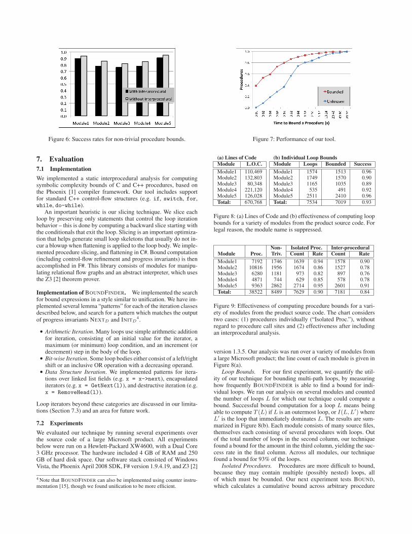
Figure 6: Success rates for non-trivial procedure bounds.

7. Evaluation

7.1 Implementation

We implemented a static interprocedural analysis for computingsymbolic complexity bounds of C and C++ procedures, based onthe Phoenix [1] compiler framework. Our tool includes supportfor standard C++ control-flow structures (e.g. if, switch, for,while, do-while).

An important heuristic is our slicing technique. We slice eachloop by preserving only statements that control the loop iterationbehavior – this is done by computing a backward slice starting withthe conditionals that exit the loop. Slicing is an important optimiza-tion that helps generate small loop skeletons that usually do not in-cur a blowup when flattening is applied to the loop body. We imple-mented procedure slicing, and flattening in C#. Bound computation(including control-flow refinement and progress invariants) is thenaccomplished in F#. This library consists of modules for manipu-lating relational flow graphs and an abstract interpreter, which usesthe Z3 [2] theorem prover.

Implementation of BOUNDFINDER. We implemented the searchfor bound expressions in a style similar to unification. We have im-plemented several lemma “patterns” for each of the iteration classesdescribed below, and search for a pattern which matches the outputof progress invariants NEXTD and INITD

4.

• Arithmetic Iteration. Many loops use simple arithmetic additionfor iteration, consisting of an initial value for the iterator, amaximum (or minimum) loop condition, and an increment (ordecrement) step in the body of the loop.

• Bit-wise Iteration. Some loop bodies either consist of a left/rightshift or an inclusive OR operation with a decreasing operand.

• Data Structure Iteration. We implemented patterns for itera-tions over linked list fields (e.g. x = x->next), encapsulatediterators (e.g. x = GetNext(l)), and destructive iteration (e.g.x = RemoveHead(l)).

Loop iterators beyond these categories are discussed in our limita-tions (Section 7.3) and an area for future work.

7.2 Experiments

We evaluated our technique by running several experiments overthe source code of a large Microsoft product. All experimentsbelow were run on a Hewlett-Packard XW4600, with a Dual Core3 GHz processor. The hardware included 4 GB of RAM and 250GB of hard disk space. Our software stack consisted of WindowsVista, the Phoenix April 2008 SDK, F# version 1.9.4.19, and Z3 [2]

4 Note that BOUNDFINDER can also be implemented using counter instru-mentation [15], though we found unification to be more efficient.

Figure 7: Performance of our tool.

(a) Lines of Code

Module L.O.C.

Module1 110,469Module2 132,803Module3 80,348Module4 221,120Module5 126,028Total: 670,768

(b) Individual Loop Bounds

Module Loops Bounded Success

Module1 1574 1513 0.96Module2 1749 1570 0.90Module3 1165 1035 0.89Module4 535 491 0.92Module5 2511 2410 0.96Total: 7534 7019 0.93

Figure 8: (a) Lines of Code and (b) effectiveness of computing loopbounds for a variety of modules from the product source code. Forlegal reason, the module name is suppressed.

Non- Isolated Proc. Inter-proceduralModule Proc. Triv. Count Rate Count Rate

Module1 7192 1746 1639 0.94 1578 0.90Module2 10816 1956 1674 0.86 1527 0.78Module3 6280 1181 973 0.82 897 0.76Module4 4871 744 629 0.85 578 0.78Module5 9363 2862 2714 0.95 2601 0.91Total: 38522 8489 7629 0.90 7181 0.84

Figure 9: Effectiveness of computing procedure bounds for a vari-ety of modules from the product source code. The chart considerstwo cases: (1) procedures individually (“Isolated Proc.”), withoutregard to procedure call sites and (2) effectiveness after includingan interprocedural analysis.

version 1.3.5. Our analysis was run over a variety of modules froma large Microsoft product; the line count of each module is given inFigure 8(a).

Loop Bounds. For our first experiment, we quantify the util-ity of our technique for bounding multi-path loops, by measuringhow frequently BOUNDFINDER is able to find a bound for indi-vidual loops. We ran our analysis on several modules and countedthe number of loops L for which our technique could compute abound. Successful bound computation for a loop L means beingable to compute T (L) if L is an outermost loop, or I(L, L′) whereL′ is the loop that immediately dominates L. The results are sum-marized in Figure 8(b). Each module consists of many source files,themselves each consisting of several procedures with loops. Outof the total number of loops in the second column, our techniquefound a bound for the amount in the third column, yielding the suc-cess rate in the final column. Across all modules, our techniquefound a bound for 93% of the loops.

Isolated Procedures. Procedures are more difficult to bound,because they may contain multiple (possibly nested) loops, allof which must be bounded. Our next experiment tests BOUND,which calculates a cumulative bound across arbitrary procedure

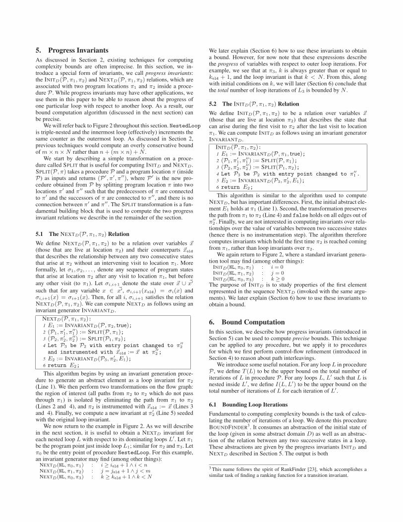
structures. To study this problem, we measured our tool’s ability tocompute a bound for individual procedures, without regard to callsites to other procedures. Many procedures are trivial (contain noloops), so our analysis focuses on the non-trivial procedures. Theresults of our experiment for several of the largest modules is givenin Figure 9 (and pictorially in Figure 6) labeled “Isolated Proc.”

Inter-procedural Analysis. We then evaluated the effective-ness of our inter-procedural technique, which properly accountsthe cost of call sites (see Section 6.4). While this is a more accuratemeasure of a procedure’s cost, it decreased our success rate to 84%.This is because of a “cascade effect”: if we fail to compute a boundfor procedure A, then any other procedure B that involves a callsite to A will also be unbounded. The results of this experiment arealso given in Figures 9 and 6, labeled “Inter-procedural.”

Limitation. One experimental limitation is that, due to the sizeof the source, we were unable to comprehensively check the pre-cision of the complexity bounds. However, we manually inspectedmany of the bounds and confirmed that they were, indeed, precise.

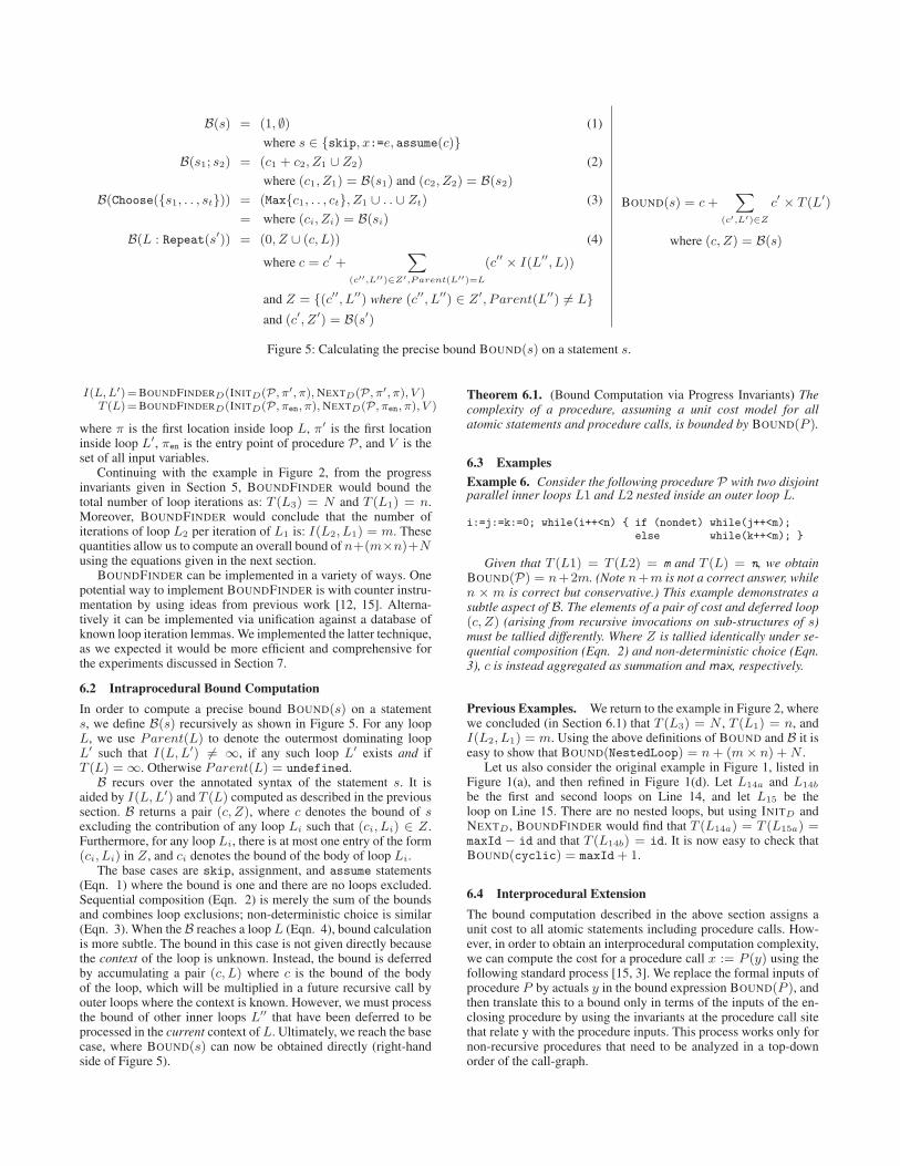
Performance. For each non-trivial procedure we also mea-sured the time it took to find a bound for the flattened version ofthe procedure. This includes control-path refinement via REFINE,progress invariant generation via INITD and NEXTD (which useINVARIANTD), finding loop bounds via BOUNDFINDER, and fi-nally calculating the total bound via BOUND. Across all modules,the performance is given in Figure 7. This graph illustrates the timeit takes to find a bound for a single procedure (in seconds). A per-fectly efficient tool would calculate bounds for 100% of proceduresinstantly. When our technique is successful, over 90% of proce-dures are bounded within 640ms. For failed attempts, only 70% ofprocedures are bounded with 640ms. This suggests a possible im-provement in the performance of our tool by aborting the search fora bound after, say, 640ms.

Figure 7 also illustrates the efficacy of our slicing heuristic.Most non-trivial functions have at most 8 paths after slicing; thusour algorithm typically completes in a fraction of a second. In lessthan 10 cases (among the 670,000 lines of code we evaluated) thenumber of paths was large enough for the analysis to time-out.

7.3 Limitations

There are some loops (roughly 7%) for which our tool is unable tofind a bound. As with any large code base, the modules vary in cod-ing styles and paradigms, yet we were surprised by how widely ap-plicable our technique was. We categorized the unsuccessful loops(somewhat automatically) into the following challenges, postponedto future work:

• Concurrency. Many procedures contained concurrent algo-rithms, such as spin-locks or work queues, in which case thethe number of loop iterations depends on other threads.

• I/O. Some modules contained procedures which interacted withthe filesystem. In these rare cases, the bound again depends onthe size (or availability) of non-deterministic input.

• Recursion. We currently do not address the issue of computingbounds for recursive procedures (though we believe that ideaspresented in this paper can potentially be used to computebounds for recursive procedures).

• Procedure Calls. Usually, procedure calls inside a loop do notaffect the value of loop iterators. But when they do, we caneither inline the appropriately sliced version of the procedure,or use an interprocedural invariant generation tool. We currentlydo not implement any such strategy.

• Exponential Paths. Slicing drastically reduces the number ofpaths in a flattened loop body; however, in rare cases, flatteninggenerates an intractable, exponential number of paths.

8. Other Application: Safety Properties

The control-flow refinement technique presented in Section 4 ismore fundamental than the sole application of bound analysis. Inparticular, it can be used to prove safety properties that otherwiserequire disjunctive invariants or a path-sensitive analysis. For thispurpose, we simply use a given simple (path-insensitive) invariantgeneration tool I to first refine the control-flow of the procedure,and then analyze the refined procedure using I .

We need a small extension of our control-flow refinement algo-rithm described in Figure 3 for it to be powerful enough to establishnon-trivial safety properties at the end of the loop. We explicitlyadd any post-dominating assume statement at the end of the multi-path loop to all top-level choices in the expansion of the loop. Thisis done to enable a path-insensitive invariant generation tool to fil-ter out paths that leave the loop prematurely. This extension is notrequired for bound analysis because the focus there was to reasonabout what happens inside the loop, and not outside the loop.

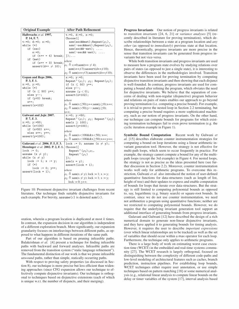
Figure 10 presents a list of some examples, each of which hasbeen used as a flagship example to motivate a new technique forproving non-trivial safety assertions. Proving validity of the asser-tions in all these examples requires disjunctive loop invariants.

Figure 10 also shows the resulting (semantically equivalent)procedure after control-flow refinement is applied using either theoctagonal [22] or polyhedra [26] analysis as the invariant genera-tion tool. The safety assertions in all these procedures can now bevalidated by running either the octagonal or the polyhedra analysison the control-refined procedure. (Note that running these analyseson the original procedure would fail to validate any of these as-sertions with the exception that octagonal domain can validate theassertion in the last procedure.) For the first example, the (induc-tive) loop invariants d = t ≤ 3 and d = s ≤ 2 for the loopsRepeat(ρ1) and Repeat(ρ2) respectively imply the assertion. Thedotted portion denotes irrelevant code that does not contain any as-sertions.

For the second example, the loop invariant x = y ∧ x ≤ 50for the first loop Repeat+(ρ1) helps establish x = y = 51 at theend of the loop; and then the loop invariant x + y = 102 ∧ x ≥52 ∧ y ≥ 0 for the second loop Repeat(ρ2) helps establish thedesired assertion after the loop. For the third example, the loopinvariant x ≤ 50 ∧ y = 50 for the first loop helps establishx = y = 50 at the end of the first loop Repeat+(ρ1), and theloop invariant x = y ∧ x ≤ 100 for the second loop Repeat+(ρ2)helps establish y = 100 at the end of the second loop. For thefourth example, the assertion is trivially established.

For the last example, the invariant x ≤ y gets established afterthe inner loop on ρ2, which then propagates itself as the loopinvariant for the outer loop too.

9. Related Work

Control Flow Refinement Control-flow refinement is related toother approaches that have been proposed for doing a more pre-cise program analysis given an underlying invariant generationtool. This includes widening strategies (such as “look-ahead widen-ing” [10] and “upto widening” [17]) or disjunctive extensions ofdomains [13, 25, 11, 14]. The primary goal of these techniquesis to compute precise invariants at different program points in theoriginal program, while we instead focus on creating a precise ex-pansion of the program into one with simpler loops. Our tech-nique is useful for bound computation, a process that is more ef-fective for simple loops, as opposed to complex loops annotatedwith precise invariants. Other work [25] does a CFG elaboration,but only as a means to perform efficient computation over somerefinement of the powerset extension. In particular k bounded elab-

Original Example After Path Refinement

Halbwachs et al. 1997,P. 14, F. 7.

t:=0; d:=0; s:=0;while (*)

if (sec)s:=0;if (t++ = 4) break;

if (met)if (s++ = 3) break;assert(d++ 6= 10);

t:=0, d:=0, s:=0;Choose({

asm(sec&&met);Repeat(ρ1),asm(¬sec&&met);Repeat(ρ2),asm(sec&&¬met); ....asm(¬sec&&¬met); ....

});...

where

ρ1 , s:=0;asm(t++ 6= 4);

asm(s++6=3);assert(d++6=10);

ρ2 , asm(s++6=3);assert(d++6=10);

Gopan and Reps 2006,P. 3, F. 1.

x:=0, y:=0;while (*)

if (x ≤ 50) y++;else y--;if (y<0) break;x++;

assert(x=102)

x:=0; y:=0;

Repeat+(ρ1); ρ2; Repeat(ρ2);if (x ≤ 50) y++;else y--;assume (y < 0);assert(x=102);

where

ρ1 , asm(x≤50);y++;asm(y≥0);x++;

ρ2 , asm(x>50);y--;asm(y≥0);

x++;Gulwani and Jojic 2007.

P. 7, F. 3.

x:=0; y:=50;while (x<100)

if (x<50) x++;else x++; y++;

assert(y=100);

x:=0; y:=50;

Repeat+(ρ1); ρ2; Repeat+(ρ2);asm(x ≥ 100);assert(y=100);

where

ρ1 , asm(x<100&&x<50); x++;

ρ2 , asm(x<100&&x≥50);x++;y++;

Gulavani et al. 2006. P. 5, F. 3.Henzinger et al. 2002. P. 2, F. 1.

lock := 0;assume (x 6= y);while (x 6= y)

lock := 1; x := y;if (*)

lock := 0; y++;assert(lock = 1);

lock := 0; assume (x 6= y);Choose({

Repeat+(ρ2);ρ1,

Repeat+(ρ1)});asm(x = y);assert(lock = 1);

where

ρ1 , asm(x 6= y); lock := 1; x := y;

ρ2 , asm(x 6= y); lock := 1; x := y;

lock := 0; y++;

Figure 10: Prominent disjunctive invariant challenges from recentliterature. Our technique finds suitable disjunctive invariants foreach example. For brevity, assume(c) is denoted asm(c).

oration, wherein a program location is duplicated at most k times.In contrast, the expansion decision in our algorithm is independentof a different exploration branch. More significantly, our expansiongranularity focuses on interleavings between different paths, as op-posed to what happens in different iterations of the same path.

Part of our algorithm is based on pruning infeasible paths.Balakrishnan et al. [4] present a technique for finding infeasiblepaths with backward and forward analyses. Infeasible paths areremoved from the transition system (“static language refinement”).The fundamental distinction of our work is that we prune infeasibleunwound paths, rather than simple, statically occurring paths.

With respect to proving safety properties (as discussed in Sec-tion 8), our technique is more precise but less efficient than widen-ing approaches (since CFG expansion allows our technique to ef-fectively compute disjunctive invariants). Our technique is orthog-onal to techniques based on disjunctive extensions (each of whichis unique w.r.t. the number of disjuncts, and their merging).

Progress Invariants Our notion of progress invariants is relatedto transition invariants [24, 6, 21] or variance analyses [5] (re-cently described in literature for proving termination), which de-scribe relationships between a state at a program location and anyother (as opposed to immediately) previous state at that location.Hence, theoretically, progress invariants are more precise in thesense that transition invariants can be generated from progress in-variants but not vice-versa.

While both transition invariants and progress invariants are usedto measure how a program state evolves by studying relations overpairs of states (as opposed to just a single state), it is interesting toobserve the differences in the methodologies involved. Transitioninvariants have been used for proving termination by computingdisjunctive transition invariants and then showing that each disjunctis well-founded. In contrast, progress invariants are used for com-puting a bound after refining the program, which obviates the needfor disjunctive invariants. We believe that the separation of con-cerns of dealing with non-regular (disjunctive) program behaviorand relations on pairs of states enables our approach to go beyondproving termination (i.e. computing a precise bound). For example,it is trivial to prove the nested loop in Section 2.2 terminating, butcomputing a precise bound requires a more sophisticated machin-ery, such as our notion of progress invariants. On the other hand,our technique can compute bounds for programs for which exist-ing termination techniques fail to even prove termination (e.g. thecyclic iteration example in Figure 1).

Symbolic Bound Computation Recent work by Gulwani etal. [15] describes elaborate counter instrumentation strategies forcomputing a bound on loop iterations using a linear arithmetic in-variant generation tool. However, the strategy is not effective formulti-path loops, which seem to occur frequently in practice. Forexample, the strategy cannot compute a bound for any of the multi-path loops (except the 3rd example) in Figure 4. For nested loops,the strategy is not as precise as the ideas presented here (see fur-ther discussion in Section 2.2). Moreover, counter instrumentationworks well only for arithmetic programs. To overcome this re-striction, Gulwani et al. also introduced the notion of user-definedquantitative functions for data-structures (such as length of list,height of tree) and their updates to express and enable computationof bounds for loops that iterate over data-structures. But the strat-egy is still limited to computing polynomial bounds as opposedto, say, logarithmic (e.g. binary search) or square-root bounds. Incontrast, since we do not use counter instrumentation, we neednot arithmetize a program using quantitative functions; neither arewe restricted to computing polynomial bounds. However, we dorequire that the underlying invariant generation tool support anadditional interface of generating bounds from progress invariants.

Gulavani and Gulwani [12] have described the design of a richnumerical domain to generate non-linear disjunctive invariants,and they have applied it to generating bounds for timing analysis.However, it requires the user to describe important expressions(over which linear relationships are to be tracked) as well as the setof variables that should occur within a max operator for each loop.Furthermore, the technique only applies to arithmetic programs.

There is a large body of work on estimating worst case execu-tion time (WCET) in the embedded and real-time systems commu-nity [27]. The WCET research is largely orthogonal, focused ondistinguishing between the complexity of different code-paths andlow-level modeling of architectural features such as caches, branchprediction, instruction pipelines. For establishing loop bounds,WCET techniques either require user annotation, or use simpletechniques based on pattern matching [18] or some numerical anal-ysis (e.g., relational linear analysis to compute linear bounds on thedelay or timer variables of the system [17], interval analysis based

approach [16], and symbolic computation of integer points in apolyhedra [20]). These WCET techniques cannot compute precisebounds for the examples considered in this paper.

Goldsmith et al. [9] compute symbolic bounds by curve-fittingtiming data obtained from profiling. Their technique has the advan-tage of measuring real amortized complexity; however the resultsare not sound for all inputs. Crary Weirich [8] presents a type sys-tem for certifying (as opposed to inferring) resource consumption,including time.

10. Conclusion and Future Work

We have introduced novel techniques for automatically determin-ing symbolic complexity bounds of procedures. We first showedhow control-flow refinement enables standard invariant generatorsto reason about mildly complex control-flow, which would other-wise require impractical disjunctive invariants. For example, wehave proven symbolic complexity bounds for procedures which noprevious technique can even prove termination. We then introducedprogress invariants and showed how to use them to compute preciseprocedure bounds. Finally, our experience with a large Microsoftproduct illustrates the effectiveness of our techniques: our tool wasable to find bounds for 90% of procedures that involve loops.

We believe that a productive direction for future work wouldbe to study broader applications for control-flow refinement andprogress invariants. As discussed in Section 8 there seem to beapplications in proving safety as well as liveness properties.

Acknowledgments. We thank Matthew Parkinson and the anony-mous reviewers for their valuable feedback which improved thispaper. We also thank the product teams at Microsoft for their as-sistance with this project and acknowledge funding from a Gatesscholarship (Koskinen).

References[1] Phoenix Compiler. research.microsoft.com/Phoenix/.

[2] Z3 Theorem Prover. research.microsoft.com/projects/Z3/.

[3] Elvira Albert, Puri Arenas, Samir Genaim, and German Puebla.Automatic inference of upper bounds for recurrence relations incost analysis. In SAS, 2008.

[4] G. Balakrishnan, S. Sankaranarayanan, F. Ivancic, O. Wei, andA. Gupta. SLR: Path-sensitive analysis through infeasible-pathdetection and syntactic language refinement. Lecture Notes inComputer Science, 5079, 2008.

[5] Josh Berdine, Aziem Chawdhary, Byron Cook, Dino Distefano, andPeter W. O’Hearn. Variance analyses from invariance analyses. InPOPL, 2007.

[6] Byron Cook, Andreas Podelski, and Andrey Rybalchenko. Termina-tion proofs for systems code. In PLDI, 2006.

[7] Patrick Cousot and Nicolas Halbwachs. Automatic discovery of linearrestraints among variables of a program. In POPL, 1978.

[8] Karl Crary and Stephanie Weirich. Resource bound certification. InPOPL, 2000.

[9] Simon Goldsmith, Alex Aiken, and Daniel Shawcross Wilkerson.Measuring empirical computational complexity. In ESEC/SIGSOFTFSE, 2007.

[10] Denis Gopan and Thomas W. Reps. Lookahead widening. In CAV,2006.

[11] Denis Gopan and Thomas W. Reps. Guided static analysis. In SAS,2007.

[12] Bhargav S. Gulavani and Sumit Gulwani. A numerical abstract domainbased on expression abstraction and max operator with application intiming analysis. In CAV, 2008.

[13] Bhargav S. Gulavani, Thomas A. Henzinger, Yamini Kannan,Aditya V. Nori, and Sriram K. Rajamani. SYNERGY: A newalgorithm for property checking. In FSE, 2006.

[14] Sumit Gulwani and Nebojsa Jojic. Program verification as probabilis-tic inference. In POPL, 2007.

[15] Sumit Gulwani, Krishna Mehra, and Trishul Chilimbi. SPEED:Precise and efficient static estimation of program computationalcomplexity. In POPL, 2009.

[16] Jan Gustafsson, Andreas Ermedahl, Christer Sandberg, and BjornLisper. Automatic derivation of loop bounds and infeasible paths forwcet analysis using abstract execution. In RTSS, 2006.

[17] Nicolas Halbwachs, Yann-Erick Proy, and Patrick Roumanoff.Verification of real-time systems using linear relation analysis. FMSD,1997.

[18] Christopher A. Healy, Mikael Sjodin, Viresh Rustagi, David B.Whalley, and Robert van Engelen. Supporting timing analysis byautomatic bounding of loop iterations. Real-Time Systems, 18(2/3),2000.

[19] Thomas A. Henzinger, Ranjit Jhala, Rupak Majumdar, and GregoireSutre. Lazy abstraction. In POPL, 2002.

[20] Bjorn Lisper. Fully automatic, parametric worst-case execution timeanalysis. In WCET, 2003.

[21] Ali Mili. Reflexive transitive loop invariants: A basis for computingloop functions. In WING, 2007.

[22] Antoine Mine. The Octagon Abstract Domain. Higher-Order andSymbolic Computation, 19(1), 2006.

[23] A. Podelski and A. Rybalchenko. A complete method for the synthesisof linear ranking functions. LNCS, 2003.

[24] A. Podelski and A. Rybalchenko. Transition invariants. In LICS,2004.

[25] Sriram Sankaranarayanan, Franjo Ivancic, Ilya Shlyakhter, and AartiGupta. Static analysis in disjunctive numerical domains. In SAS,2006.

[26] Chao Wang, Zijiang Yang, Aarti Gupta, and Franjo Ivancic. Usingcounterexamples for improving the precision of reachability compu-tation with polyhedra. In CAV, 2007.

[27] Reinhard Wilhelm, Jakob Engblom, Andreas Ermedahl, NiklasHolsti, Stephan Thesing, David Whalley, Guillem Bernat, ChristianFerdinand, Reinhold Heckmann, Frank Mueller, Isabelle Puaut, PeterPuschner, Jan Staschulat, and Per Stenstrom. The Determination ofWorst-Case Execution Times—Overview of the Methods and Surveyof Tools. In TECS, 2007.