B.Tech Project

Adaptive Grid Refinement in Incompressible Flow

by:

Abhishek Yamini (Roll no. 2009002)

Himanshu Singh (Roll no. 2009039)

under the supervision of

Dr. Goutam Dutta

DEPARTMENT OF MECHANICAL ENGINEERING

INDIAN INSTITUTE OF INFORMATION TECHNOLOGY,

DESIGN AND MANUFACTURING JABALPUR

INDIA

November13,2012

Acknowledgement

We would like to express our gratitude to our Academic mentor

Dr. Gautam Dutta for his sincere help in each and every phase of our progress in this

project .Without his continuous support and guidance as well as his encouragement during

difficult periods, the completion of our 6-Month B.Tech Project Report would not have

been possible , we would also like to thank all the professors who increased our knowledge in

many areas, and who always gave insightful responses to any questions and concerns. we

would like to thank my fellow students who always offered their help. Even the smallest

discussion would always introduce new ideas on how to overcome a problem.

iii

Abstract

The overall objective of the present research work is to solve the physical problem

related to fluid dynamics of incompresible isotropic type of fluids , what happens in any industry

they have big plants in which they perform wind tunnel testing and so many which are obiviously

so much coastly and time consuming . Many great Scientists and various researh scholars have

already contributed so much in relating variation of such physical variation of fluids with

Mathematics. Thus the concept of "Computational Fluid Dynamics" motivated us to work in

this field, during the period of six month of our B.tech Project we have learned many interesting

algorithms and several fundamental properties of various kinds of fluid flow , we developed our

flexible computational programmes which can solve Navier Stokes Equation for incompressible

flows accompanied with different boundary conditions across any finite control volume. We have

adopted the concept of SIMPLE-Method given by Patnakar[3] for collocated grid although the

SIMPLE-staggered grid method enjoyed considerable success particularly when Cartesian grids

were employed, but the procedure was found to be inconvenient when curvilinear or adaptive

grids were to be employed to compute over more complex domains. It was found that if the

pressure correction equation as derived for staggered grids was used to predict pressure on

collocated grids the resulting pressure distribution showed zig-zagness. Here we shall describe the

method proposed by

A.W Date [1]that elegantly eliminates the problem of zigzag pressure prediction

. Later we have discussed about the Advance topic in CFD "The Concept of Adaptive Grid"

, the beauty of adaptive grid is that it adjust physical plane in such a way so that it represent the

dynamic variation occurring because of gradient of some physical quantities on Cartesian plane,

for obtaining these values in curvilinear co-ordinate system we have to solve Navier-Stokes

equations of mass, momentum and energy for compressible and viscous fluid.

Keywords: Incompressible Fluid, Isentropic Fluid, Wind Tunnel Testing, CFD, Navier

Stokes Equations, SIMPLE Method, Cartesian Grid, Curvilinear Grid, Staggered Grid,

Collocated Grid, Adaptive Grid

Nomenclature

English symbols

Qx Heat Flux

A Area (m2)

Density of Fluid

c Heat capacity

T Temperature

wx Distance between west and central node

ex Distance between east and central node

nx Distance between north and central node

sx Distance between south and central node

x Distance between east and west node

k Thermal conductivity

'''q Heat generation Term

t Small time period

TE Temperature at East node

TP Temperature at central node

TW Temperature at west node

TN Temperature at north node

TS Temperature at south node

Constant quantity n

ET New value of Temperature at East node

n

PT New value of Temperature at central node

n

WT New value of Temperature at west node

n

ST New Temperature at south node

Field value

wWx Distance between west cell face and west node

wPx Distance between west cell face and central node

v

wEx Distance between west cell face and central node

eEx Distance between west cell face and central node

J Total flux across vontrol volume

J*

Non-dimensionalise value of total flux

P Peclet Number

R Reynold Number

SUBSCRIPTS

1 Lower Attachment Point

2 Upper Detachment Point

3 Upper Attachment Point

E East Side Node

EE East Side Upstream Node

e E ast Side Control Volume Face

i Velocity Grid Point in x-Direction

I Scalar Node in x-Direction

J Total Flux

j Velocity Grid Point in y-Direction

J Scalar Node in y-Direction

n North Side Control Volume Face

N North Side Node

nb Neighbor Cells

P General Nodal Point

S South Side Node

s South Side Control Volume Face

u x (Axial ) Component

v y (Tangential) Component

W West Side Node

WW West Side Upstream Node

w West Side Control Volume Face

Contents

Nomenclature…………………………………………………………………iv

Chapter 1:

1.1 Heat Conduction in One dimension……………………………………….(1)

1.2 Discretization of one dimensional domain………………………………..(3)

1.2(a) Finite difference method using taylor series……………………………(3)

1.2(b) Finite volume method …………………………………………………(6)

1.3 Heat conduction in two dimension………………………………………..(8)

1.3 (A) ) Finite volume Approach in Two Dimension………………………..(8)

1.4 Solution methodology for Non-linear implicit scheme………………......(11)

1.5 Results and discussions…………………………………………………...(12)

1.5 Comparision b/w Implicit and Analytical Solution in One Dimension......(12)

1.6 Analysis Of two dimension heat conduction……...……………………...(15)

Chapter 2:

One Dimension Convection: Interpolation model for CFD

2.1 Concept Of finite volume method …………..……………………...........(18)

2.2 Convection-Diffusion Equation ………………………………………….(19)

2.3 The Finite volume mesh……………………………………………….....(20)

2.4 Advection-Diffusion Equation for one dimension steady state…………..(21)

2.4.1Central Difference scheme……………………...……………………….(22)

2.4.2Up-wind differencingscheme…………………………………………...(26)

2.4.2.1 Assesments of Up-wind differencingscheme……………………...…(28)

2.4.3 Hybrid scheme………………………………………...……………….(31)

vii

Chapter3:

Conconcept of Stream-vorticity Method

3.1 Stream function………………………………..…………………….........(34)

3.2 Vorticity…………………………………………………………………..(35)

3.3 Solution methodology for solving Lid-Driven Cavity problem using stream-

vorticity method…………………………………............................................(36)

Chapter 4

4.1 Two dimensional convectional diffusion equation…………………….....(37)

4.2 Continuity equation on control-volume…………………………………..(41)

4.3 Convection-Diffusion equation…………………………………………...(42)

4.4 Calculation of velocity field …………………………………………......(44)

4.5 SIMPLE method for staggered grid……………………………………....(46)

4.6 Solution methodology of SIMPLE……………………………………….(47)

4.7 Adaptive grid in two-dimensional boundary layer……………………….(48)

4.8 Assumption taken for alogrithm………………………………………….(49)

4.9 Algorithm…………………………………………………………………(51)

Chapter 5

Implementation of TDMA

5.1 Introduction of TDMA…………………………………………………....(53)

5.2 Implementation of sample problem……………………………..……......(53)

5.2.1 Problem Statement………..………………………………………….…(54)

5.2.2 Computational Results……………………………………………….…(54)

Chapter 6

6.1 Analysis of lid-driven cavity flow………………………………………..(58)

6.2 Algorithm………………………………………………………………....(59)

6.3 Results…………………………………………………………………….(60)

6.4 SIMPLE method for collocated grid……………………………………...(61)

6.5 Discretisation………………………………………………………….….(62)

6.6 Pressure-correction equation……………………………………………..(64)

6.7 Overall calcuation procedur………………………………………………(68)

6.8 Computational Results……………………………………………………(69)

Chapter 7

Concept of Adaptive grid

7.1 Introduction……………………………………………………………….(75)

7.2 Curvilinear Grid…………………………………………………………..(77)

7.2.1 Co-ordinate Transformation……………………………………………(77)

7.3 Transport Equation……………………………………………………….(79)

References……………………………………………………………………(82)

List of Figures

Figure:1.1a Domain of one dimension conduction…...……………….…(2)

Figure:1.2a Control volume in 1D about node "P"……...…………….....(3)

Figure:1.2b Definition of explicit scheme……………..………………...(7)

Figure:1.2b Definition of implicit scheme……………......……………...(7)

Figure:1.3a Control volume for 2D heat conduction…………………….(9)

Figure:1.5.1.a Comparision b/w analytical and implicit method using finite

volume method for one dimension……………………………………...(13)

Figure:1.5.1.b Surface plot of Temperture distribution using implicit

approach in time and space for 20 Nodes………………………………(14)

Figure:1.6.a Symmetrical plot of Temperature Distribution……………(15)

Figure:1.6.b Three dimensional plot of temperature profile w.r.t space..(16)

Figure:2.1 One dimensional control volume……………………………(20)

Figure:2.2 Comparision b/w CDS and Exact Solution…………………(25)

Figure:2.3 Oscillating Nature of CDS…………………………………..(25)

ix

Figure:2.4 Comparison b/w CDS and Analytical solution……………...(26)

Figure:2.5 Comparison b/w UDS and Analytical Solution…………….(29)

Figure:2.6 Comparison b/w UDS and Analytical Solution…………….(30)

Figure:2.7 Comparison b/w UDS and Analytical Solution…………….(31)

Figure:2.8 Comparison b/w Hybrid and Analytical Solution…………..(32)

Figure:2.8 Comparison b/w Hybrid and Analytical Solution…………..(33)

Fgure:3.1 Vorticity in given Domain with velocity Vectors at each

Node…………………………………………………………………….(34)

Figure:3.2 Contour plot of stream Function with velocity vectors at each

Node………………………………………………………………….…(38)

Figure:4.1 Two-Dimension domain for finite volume Analysis………..(41)

Figure:4.2 Pressure at nodes and velocities at cell-face………………...(44)

Figure:4.3 Two dimensional control volume…………………………...(45)

Figure:4.4 Domain of boundary layer…………………………………..(48)

Figure:4.5 Domain of Discretisation..…………………………………..(48)

Figure:5.1 Temperature Distribution within the slab…………………...(55)

Figure:5.2 Temperature Distribution as given in Reference[5]………...(56)

Figure:5.3 Solution after 37 iterations ………………………………....(57)

Figure:6.1 Comparison b/w our Results and slandered Results………...(60)

Figure:6.2 Domain of discretisation for collocated grid………………..(61)

Figure:6.3 Boundary Conditions of Lid driven cavity problem………...(69)

Figure:6.4 U-component of velocity by UDS for 129x129 Grids……...(70)

Figure:6.5 V-component of velocity by UDS for 129x129 Grids……...(70)

Figure:6.6 U-component of velocity by UDS for 129x129 Grids……...(71)

Figure:6.7 V-component of velocity by UDS for 129x129 Grids……...(71)

Figure:6.8 Error Vs Iteration by CDS for 50 x 50 Grid………………...(72)

Figure:6.9 Error Vs Iteration by Power Law for 50 x 50 Grid………....(72)

Figure:6.10 Error Vs Iteration by UDS for 50 x 50 Grid………............(73)

Figure:6.11 Comparison of V-velocities obtain by different schemes for 50

x 50 Grid Points…………………………………………………….......(73)

Figure:6.12 Comparison of U-Velocities obtain by different scheme for 50

x 50 Grid………………………………………………..………............(74)

xi

Adaptive Grid Refinement in

Incompressible Flow

1

Chapter 1

Introduction

The Fundamental property of fluid is govern by trans-portiveness nature of fluid

particles i.e by advection and diffusion . So we analyzed the heat distribution within given one

dimensional & two dimensional geometry, in which heat is defined as energy transferred to the

system by thermal interactions. Heat flows spontaneously from systems of higher temperature to

systems of lower temperature. When two systems come into thermal contact, they exchange

thermal energy due to the microscopic interactions of their particles. When the systems are at

different temperatures, the net flow of thermal energy is not zero and is directed from the hotter

region to the cooler region, until their temperatures are equal and the net flow of energy is zero.

Spontaneous heat transfer is an irreversible process, which leads to the systems coming closer to

mutual thermodynamic equilibrium. For analysis of heat conduction in 1D &2D we followed

method of finite difference and finite volume method, in both method we have two approaches

first is called “explicit approach” and another is called “implicit approach” . Finally at the end of

this section we compare each method with the help of partial differential equations by plotting

their results on MATLAB.

Literature Review

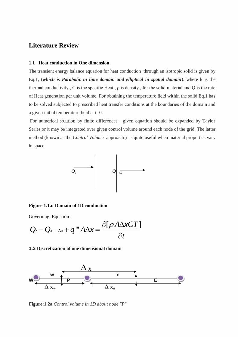
1.1 Heat conduction in One dimension

The transient energy balance equation for heat conduction through an isotropic solid is given by

Eq.1, (which is Parabolic in time domain and elliptical in spatial domain). where k is the

thermal conductivity , C is the specific Heat , ρ is density , for the solid material and Q is the rate

of Heat generation per unit volume. For obtaining the temperature field within the solid Eq.1 has

to be solved subjected to prescribed heat transfer conditions at the boundaries of the domain and

a given initial temperature field at t=0.

For numerical solution by finite differences , given equation should be expanded by Taylor

Series or it may be integrated over given control volume around each node of the grid. The latter

method (known as the Control Volume approach ) is quite useful when material properties vary

in space

xQ x xQ

Figure 1.1a: Domain of 1D conduction

Governing Equation :

[ ]'''x x x

A xCTQ Q q A x

t

1.2 Discretization of one dimensional domain

X w e W P E

Xw Xe

Figure:1.2a Control volume in 1D about node "P"

3

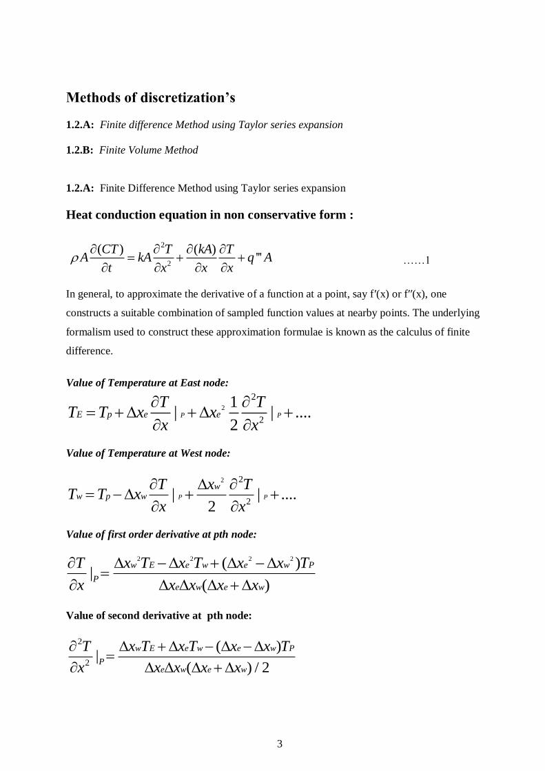
Methods of discretization’s

1.2.A: Finite difference Method using Taylor series expansion

1.2.B: Finite Volume Method

1.2.A: Finite Difference Method using Taylor series expansion

Heat conduction equation in non conservative form :

2

2

( ) ( )'''

CT T kA TA kA q A

t x x x

……1

In general, to approximate the derivative of a function at a point, say f′(x) or f′′(x), one

constructs a suitable combination of sampled function values at nearby points. The underlying

formalism used to construct these approximation formulae is known as the calculus of finite

difference.

Value of Temperature at East node:

2

2

2

1| | ....

2P PE p e e

T TT T x x

x x

Value of Temperature at West node:

2 2

2| | ....

2P P

ww p w

T x TT T x

x x

Value of first order derivative at pth node:

2 2 2 2( )|

( )

w E e w e w P

Pe w e w

T x T x T x x T

x x x x x

Value of second derivative at pth node:

2

2

( )|

( ) / 2

w E e w e w P

Pe w e w

T x T x T x x T

x x x x x

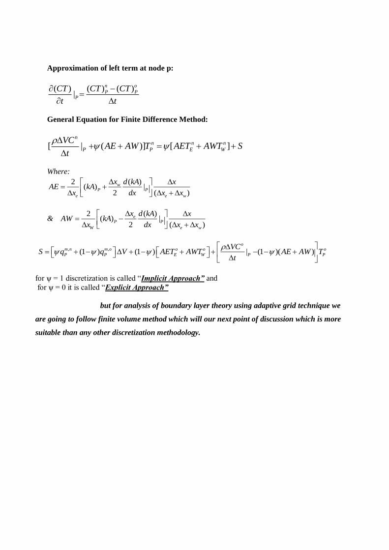
Approximation of left term at node p:

( ) ( )( )|

n o

P PP

CT CTCT

t t

General Equation for Finite Difference Method:

[ | ( )] [ ]n

n n n

P P E W

VCAE AW T AET AWT S

t

Where:

2 ( )( ) |

2 ( )

wP P

e e w

x d kA xAE kA

x dx x x

& 2 ( )

( ) |2 ( )

eP P

W e w

x d kA xAW kA

x dx x x

, ,(1 ) (1 ) | (1 )( )o

m n m o o o o

P P E W P P

VCS q q V AET AWT AE AW T

t

for ѱ = 1 discretization is called “Implicit Approach” and

for ѱ = 0 it is called “Explicit Approach”

but for analysis of boundary layer theory using adaptive grid technique we

are going to follow finite volume method which will our next point of discussion which is more

suitable than any other discretization methodology.

5

1.2.B: Finite Volume Approach in 1D

The finite volume method approximates the P.D.E. over a control volume surrounding the grid node,

rather than at the node itself. The discretisation equations are obtained by integrating the P.D.E. over

control volumes surrounding the grid nodes, after introducing necessary simplifications and

assumptions . The left term of generate heat conduction eq. for transient case , on integrating it from

old time value to new time value in time domain & from 'w' to 'e' in spatial domain:

'

( )( ) ( )

t e

n o

P pt w

CTA dxdt A x CT CT

t

And right term:

'

''' '''|

e t e

e W P

w t w

T T TkA dxdt q Adxdt kA kA t q A x t

x x x x

| , | P WE Pe w

e w

T TT TT T

x x x x

Governing equation for finite volume approach

Thus,

[ | ( )] [ ]n

n n n

P P E W

VCAE AW T AET AWT S

t

Where:

2 ( )( ) |

2 ( )

wP P

e e w

x d kA xAE kA

x dx x x

&

2 ( )( ) |

2 ( )

eP P

W e w

x d kA xAW kA

x dx x x

, ,(1 ) (1 ) | (1 )( )o

m n m o o o o

P P E W P P

VCS q q V AET AWT AE AW T

t

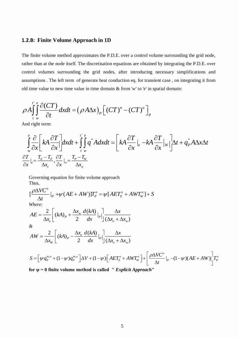
for ѱ = 0 finite volume method is called " Explicit Approach"

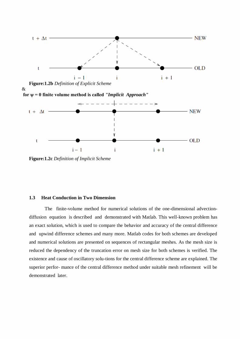
Figure:1.2b Definition of Explicit Scheme

&

for ѱ = 0 finite volume method is called "Implicit Approach"

Figure:1.2c Definition of Implicit Scheme

1.3 Heat Conduction in Two Dimension

The finite-volume method for numerical solutions of the one-dimensional advection-

diffusion equation is described and demonstrated with Matlab. This well-known problem has

an exact solution, which is used to compare the behavior and accuracy of the central difference

and upwind difference schemes and many more. Matlab codes for both schemes are developed

and numerical solutions are presented on sequences of rectangular meshes. As the mesh size is

reduced the dependency of the truncation error on mesh size for both schemes is verified. The

existence and cause of oscillatory solu-tions for the central difference scheme are explained. The

superior perfor- mance of the central difference method under suitable mesh refinement will be

demonstrated later.

7

1.3.A Finite Volume Approach in 2D

Finite volume methods are widely used in computational fluid dynamics (CFD) codes. The

elementary finite volume method uses a cell-centered mesh and finite difference approximations

of first order derivatives. This section shows how the finite volume method is applied to a

model of convective transport: the two -dimensional convection-diffusion equation.

2 2

2 20

T Tk

x y

Integrating the above equation within control volume yields:

2 2 2 2

2 2 2 20

y y y y y yx x x x x x

y x y x y x

T T T Tk dxdy k dxdy k dxdy

x y x y

(i,j+1)

(i-1,j) (i,j) (i+1,j)

(i,j-1)

Figure: 1.3.a Control Volume for 2D Heat Conduction

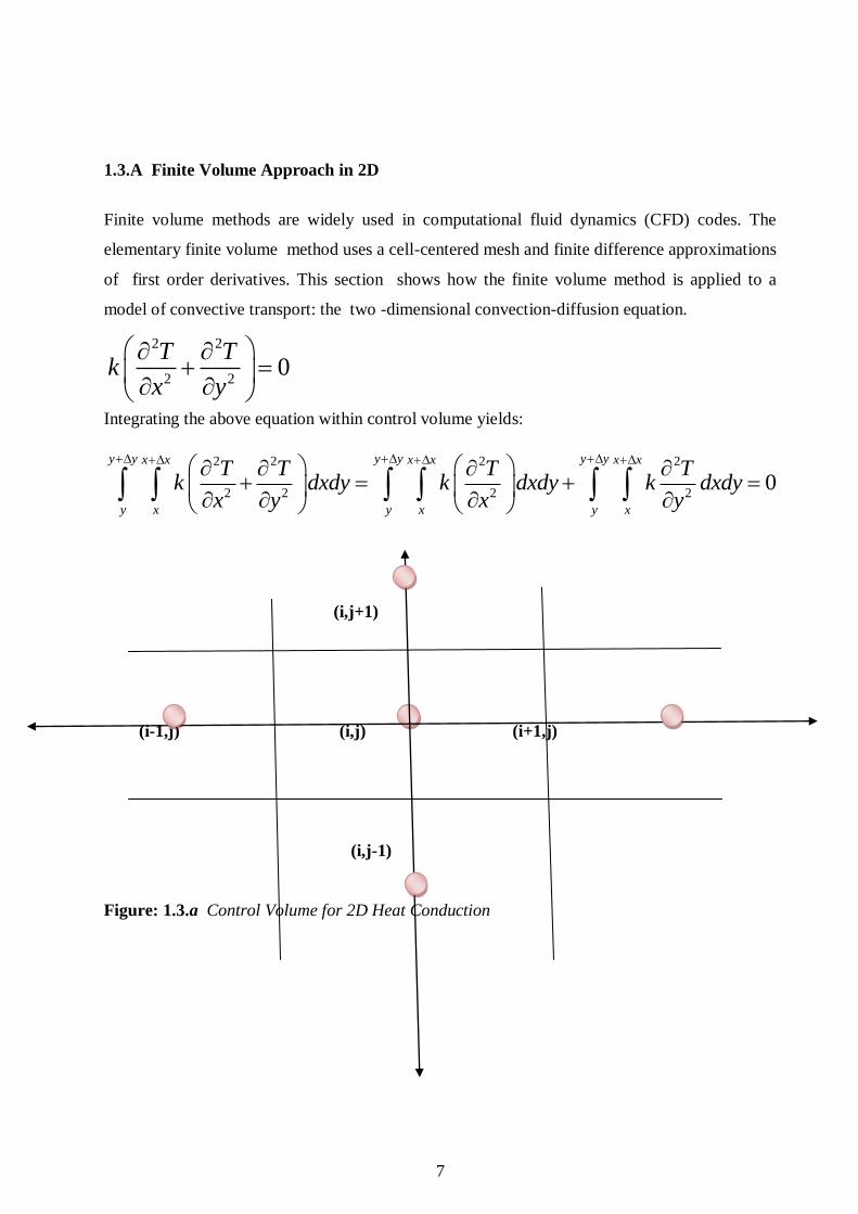
On integrating first term of above equation within given control vol:

2

2.

y y y yx x

x x xy x y

T T Tk dxdy k k dy

x x x

On integrating second term of governing equation within control vol

2

2. .

y y x x

x x xy x

T T Tk dx dy k y k y

x x x

On expanding first order term within control vol using central difference scheme

21, , , 1,

2. .

y y x xi j i j i j i j

y x

T T T TTk dx dy k y k y

x x x

2, 1 , , , 1

2. .

y y x xi j i j i j i j

y x

T T T TTk dx dy k x k x

x y y

arranging both side term, we get governing equation for 2d heat conduction using finite volume

method,

1, , , 1, , 1 , , , 10

i j i j i j i j i j i j i j i jT T T T T T T Tk y k y k x k x

x x y y

This equation will depend on boundary condition of given control volume so one should take

care in making equation at boundary nodes.

9

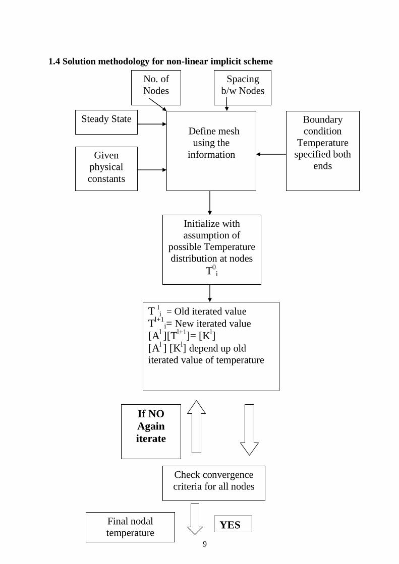
1.4 Solution methodology for non-linear implicit scheme

Steady State

No. of

Nodes

Spacing

b/w Nodes

Boundary

condition

Temperature

specified both

ends

Define mesh

using the

information Given

physical

constants

Initialize with

assumption of

possible Temperature

distribution at nodes

T0i

T li = Old iterated value

Tl+1

i= New iterated value

[Al ][T

l+1]= [K

l]

[Al ] [K

l] depend up old

iterated value of temperature

Check convergence

criteria for all nodes

If NO

Again

iterate

YES Final nodal

temperature

distribution

1.5 Results & Discussions

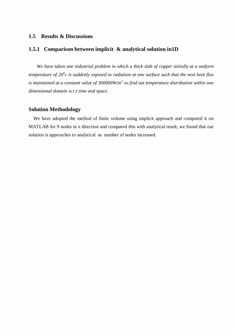
1.5.1 Comparison between implicit & analytical solution in1D

We have taken one industrial problem in which a thick slab of copper initially at a uniform

temperature of 200c is suddenly exposed to radiation at one surface such that the next heat flux

is maintained at a constant value of 300000W/m2 so find out temperature distribution within one

dimensional domain w.r.t time and space.

Solution Methodology

We have adopted the method of finite volume using implicit approach and computed it on

MATLAB for 9 nodes in x direction and compared this with analytical result, we found that our

solution is approaches to analytical as number of nodes increased.

11

Figure:1.5.1.a Comparison between analytical & implicit method using finite vol. method for

One dimension

Assumptions:For this particular problem Thermal conductivity , density and heat capacity is

not varying w.r.t space & time. Temperature is varying w.r.t time. and space.

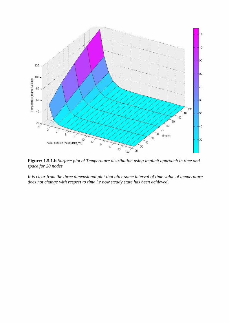
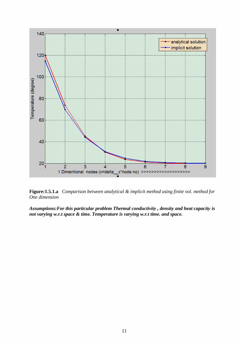
Figure: 1.5.1.b Surface plot of Temperature distribution using implicit approach in time and

space for 20 nodes

It is clear from the three dimensional plot that after some interval of time value of temperature

does not change with respect to time i.e now steady state has been achieved.

13

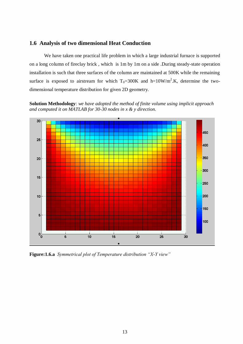
1.6 Analysis of two dimensional Heat Conduction

We have taken one practical life problem in which a large industrial furnace is supported

on a long column of fireclay brick , which is 1m by 1m on a side .During steady-state operation

installation is such that three surfaces of the column are maintained at 500K while the remaining

surface is exposed to airstream for which T0=300K and h=10W/m2.K, determine the two-

dimensional temperature distribution for given 2D geometry.

Solution Methodology: we have adopted the method of finite volume using implicit approach

and computed it on MATLAB for 30-30 nodes in x & y direction.

Figure:1.6.a Symmetrical plot of Temperature distribution “X-Y view”

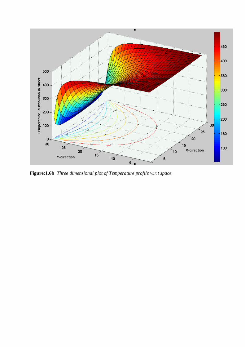
Figure:1.6b Three dimensional plot of Temperature profile w.r.t space

15

Chapter 2

One Dimensional Convection: Interpolation Models for CFD

Fnite-volume method for numerical solutions of the one-dimensional Advection – Diffusion

equation is described and demonstrated with the help of nonlinear differential equations .

Depending upon given boundary conditions such type of equations have well-known problem

that has an exact solution , which is used to compare the behavior and accuracy of the various

interpolation methods like central difference and upwind difference schemes and many more .

We have developed Matlab codes for these schemes and further numerical solution has been

obtained using finer grid points . As the mesh size is reduced the dependency of the truncation

error on mesh size for both schemes is verified. The existence and cause of oscillatory solutions

for the central difference scheme are explained. The superior performance of the central

difference method under suitable mesh refinement is demonstrated.

2.1 Concept Of Finite-Volume Method

Finite volume methods are widely used in computational fluid dynamics (CFD) codes. The

elementary finite volume method uses a cell-centered mesh and finite-difference approximations

of first order derivatives. We explained in this chapter how the finite volume method is applied

to a model of one dimension Advection –Diffusion transport phenomena .

There are two primary goals of this chapter. The first is to expose the fundamental concept of

Finite-Volume Method. Readers interested in additional details, including application to the

Navier-Stokes equations, should consult the classic text book by Patankar [Ref 3].

ANDERSON give a more up-to-date discussion of Finite volume methods, but without the low

level details presented in this section . Versteeg and Malalasekera [Ref 5] provide a detailed

discussion of the topics described in this section ,

The second goal of this chapter is to introduce and a detailed comparison between

various interpolation methods ,and why there numerical soltion starts Oscillatios.

2.2 The Convection-Diffusion Equation

The general transport equation for any fluid property is given by

div u div grad S

t

(1)

In problems where fluid flow plays a significant role we must account for the effects of

convection. Diffusion always occurs alongside convection in nature so here we examine method

to predict combined convection and Diffusion. The steady convection -diffusion equation can be

derived from

transport equation (1) for a general property by deleting transient term so we have:

div u div grad S (2)

Formal integration over a control volume gives:

. .A A CV

n u dA n grad dA S dV (3)

this equation represents the flux balance in a control volume .The left hand side gives the net

convective flux and the right side contains the net diffusive flux and the generation or

destruction of property ϕ within the control volume.

2.3 The Finite Volume Mesh

In the finite difference method, the mesh is denoted by the location of nodes in space (and

possibly time). In the finite volume method, the spatial domain of the physical problem is

subdivided into non-overlapping cells or control volumes. A single node is located at the

geometric centroid of the control volume . In the finite volume method, the numerical

approximation is obtained by integrating the governing equation over the control volume. The

nodal volumes are used to compute the flux of dependent variable from one control volume into

the next.

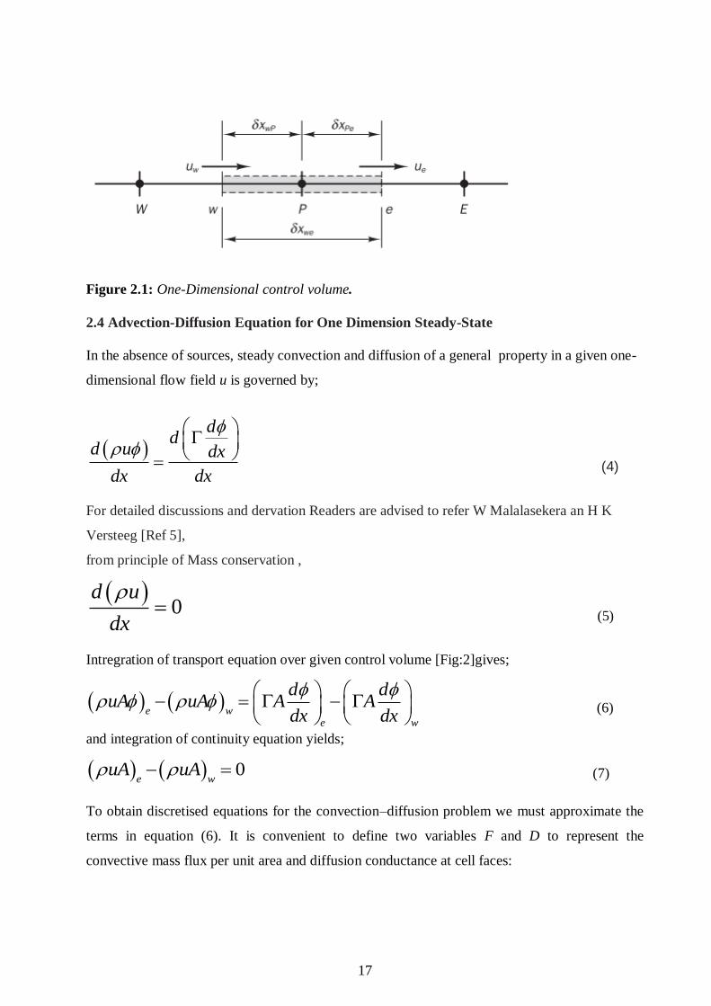
17

Figure 2.1: One-Dimensional control volume.

2.4 Advection-Diffusion Equation for One Dimension Steady-State

In the absence of sources, steady convection and diffusion of a general property in a given one-

dimensional flow field u is governed by;

d

dd u dx

dx dx

(4)

For detailed discussions and dervation Readers are advised to refer W Malalasekera an H K

Versteeg [Ref 5],

from principle of Mass conservation ,

0

d u

dx

(5)

Intregration of transport equation over given control volume [Fig:2]gives;

e w

e w

d duA uA A A

dx dx

(6)

and integration of continuity equation yields;

0e w

uA uA (7)

To obtain discretised equations for the convection–diffusion problem we must approximate the

terms in equation (6). It is convenient to define two variables F and D to represent the

convective mass flux per unit area and diffusion conductance at cell faces:

F u

Dx

So integration of convection diffusion (6) can be written as:

e e w w e e P w P wF F D D (9)

and the integrated continuity equation becomes:

0e wF F

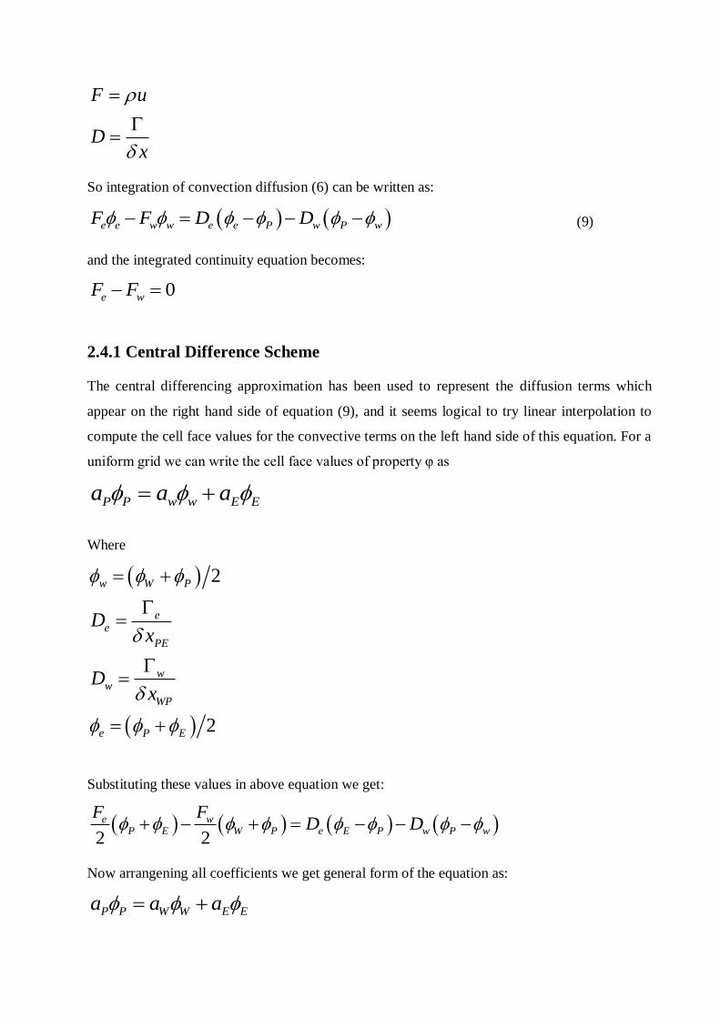
2.4.1 Central Difference Scheme

The central differencing approximation has been used to represent the diffusion terms which

appear on the right hand side of equation (9), and it seems logical to try linear interpolation to

compute the cell face values for the convective terms on the left hand side of this equation. For a

uniform grid we can write the cell face values of property φ as

P P w w E Ea a a

Where

2

2

w W P

ee

PE

ww

WP

e P E

Dx

Dx

Substituting these values in above equation we get:

2 2

e wP E W P e E P w P w

F FD D

Now arrangening all coefficients we get general form of the equation as:

P P W W E Ea a a

19

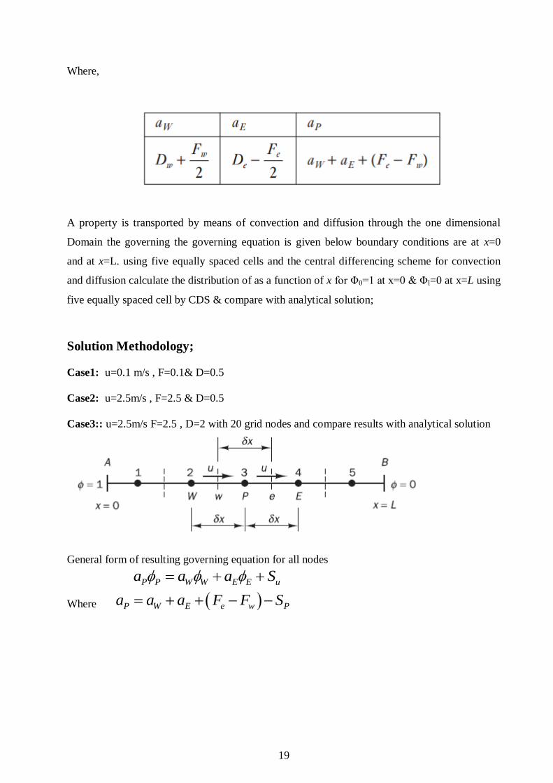
Where,

A property is transported by means of convection and diffusion through the one dimensional

Domain the governing the governing equation is given below boundary conditions are at x=0

and at x=L. using five equally spaced cells and the central differencing scheme for convection

and diffusion calculate the distribution of as a function of x for Φ0=1 at x=0 & Φl=0 at x=L using

five equally spaced cell by CDS & compare with analytical solution;

Solution Methodology;

Case1: u=0.1 m/s , F=0.1& D=0.5

Case2: u=2.5m/s , F=2.5 & D=0.5

Case3:: u=2.5m/s F=2.5 , D=2 with 20 grid nodes and compare results with analytical solution

General form of resulting governing equation for all nodes

P P W W E E ua a a S

Where P W E e w Pa a a F F S

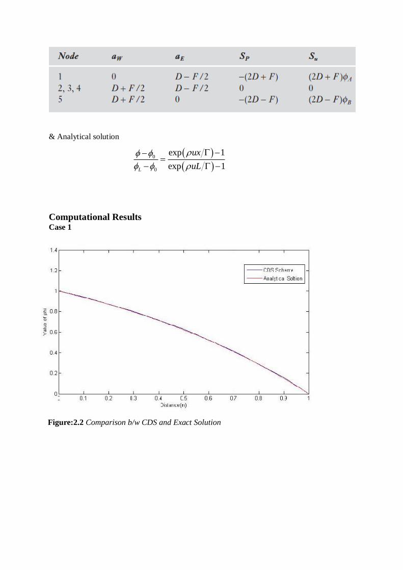
& Analytical solution

0

0

exp 1

exp 1L

ux

uL

Computational Results Case 1

Figure:2.2 Comparison b/w CDS and Exact Solution

21

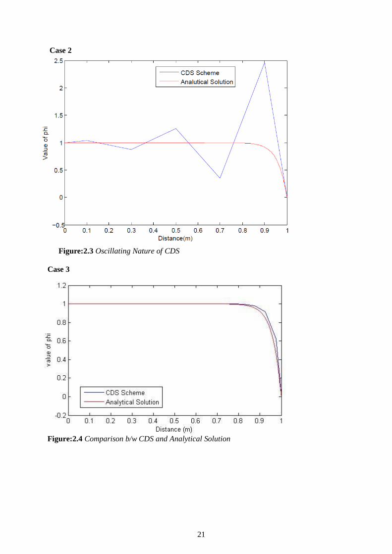
Case 2

Figure:2.3 Oscillating Nature of CDS

Case 3

Figure:2.4 Comparison b/w CDS and Analytical Solution

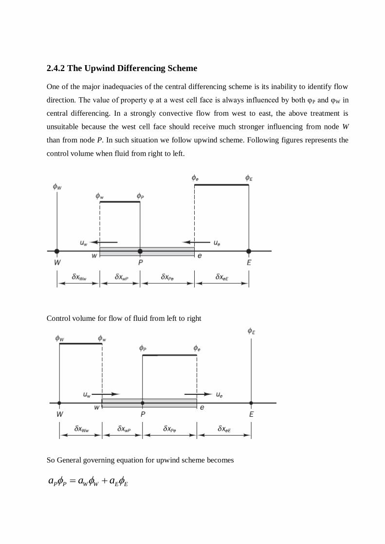
2.4.2 The Upwind Differencing Scheme

One of the major inadequacies of the central differencing scheme is its inability to identify flow

direction. The value of property φ at a west cell face is always influenced by both φP and φW in

central differencing. In a strongly convective flow from west to east, the above treatment is

unsuitable because the west cell face should receive much stronger influencing from node W

than from node P. In such situation we follow upwind scheme. Following figures represents the

control volume when fluid from right to left.

Control volume for flow of fluid from left to right

So General governing equation for upwind scheme becomes

P P W W E Ea a a

23

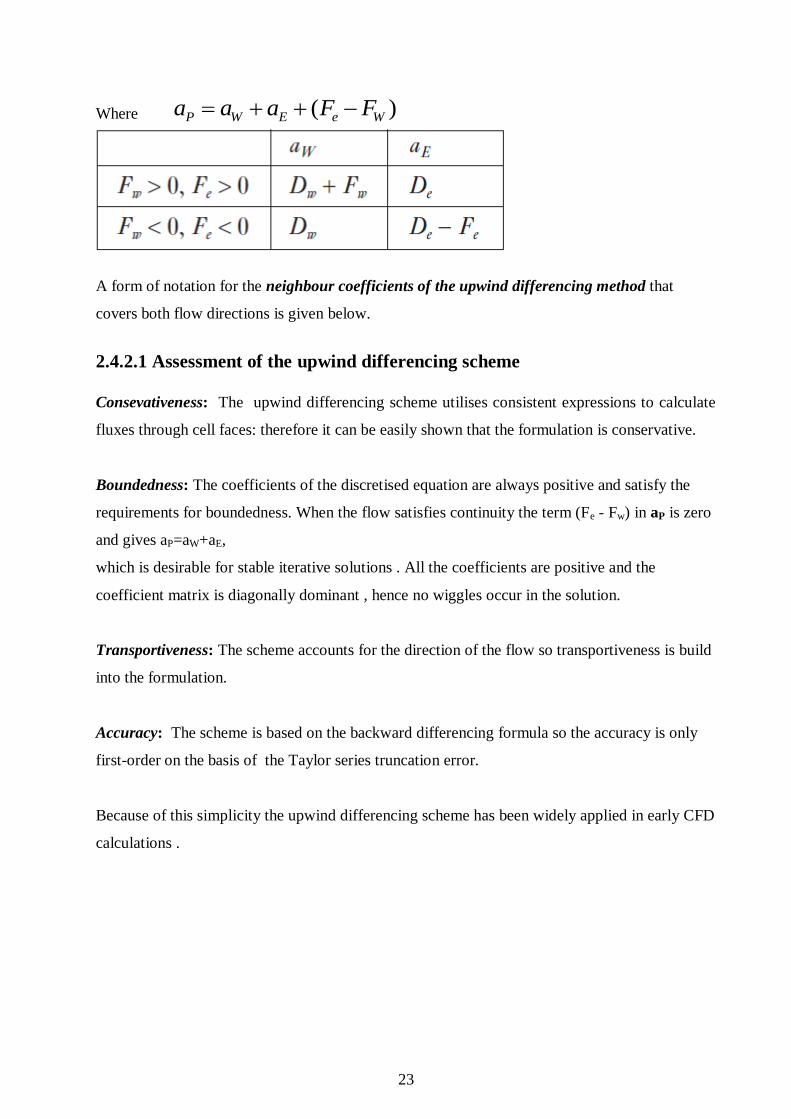
Where ( )P W E e Wa a a F F

A form of notation for the neighbour coefficients of the upwind differencing method that

covers both flow directions is given below.

2.4.2.1 Assessment of the upwind differencing scheme

Consevativeness: The upwind differencing scheme utilises consistent expressions to calculate

fluxes through cell faces: therefore it can be easily shown that the formulation is conservative.

Boundedness: The coefficients of the discretised equation are always positive and satisfy the

requirements for boundedness. When the flow satisfies continuity the term (Fe - Fw) in aP is zero

and gives aP=aW+aE,

which is desirable for stable iterative solutions . All the coefficients are positive and the

coefficient matrix is diagonally dominant , hence no wiggles occur in the solution.

Transportiveness: The scheme accounts for the direction of the flow so transportiveness is build

into the formulation.

Accuracy: The scheme is based on the backward differencing formula so the accuracy is only

first-order on the basis of the Taylor series truncation error.

Because of this simplicity the upwind differencing scheme has been widely applied in early CFD

calculations .

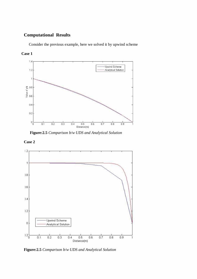
Computational Results

Consider the previous example, here we solved it by upwind scheme

Case 1

Figure:2.5 Comparison b/w UDS and Analytical Solution

Case 2

Figure:2.5 Comparison b/w UDS and Analytical Solution

25

Case 3

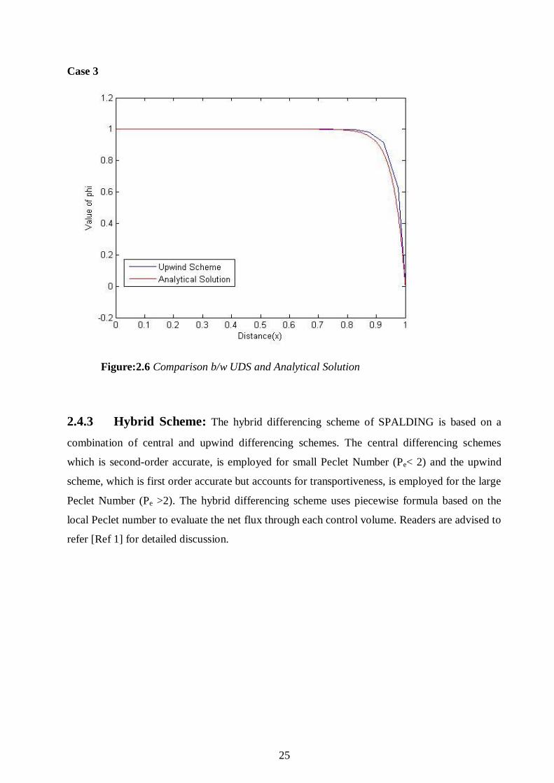
Figure:2.6 Comparison b/w UDS and Analytical Solution

2.4.3 Hybrid Scheme: The hybrid differencing scheme of SPALDING is based on a

combination of central and upwind differencing schemes. The central differencing schemes

which is second-order accurate, is employed for small Peclet Number (Pe< 2) and the upwind

scheme, which is first order accurate but accounts for transportiveness, is employed for the large

Peclet Number (Pe >2). The hybrid differencing scheme uses piecewise formula based on the

local Peclet number to evaluate the net flux through each control volume. Readers are advised to

refer [Ref 1] for detailed discussion.

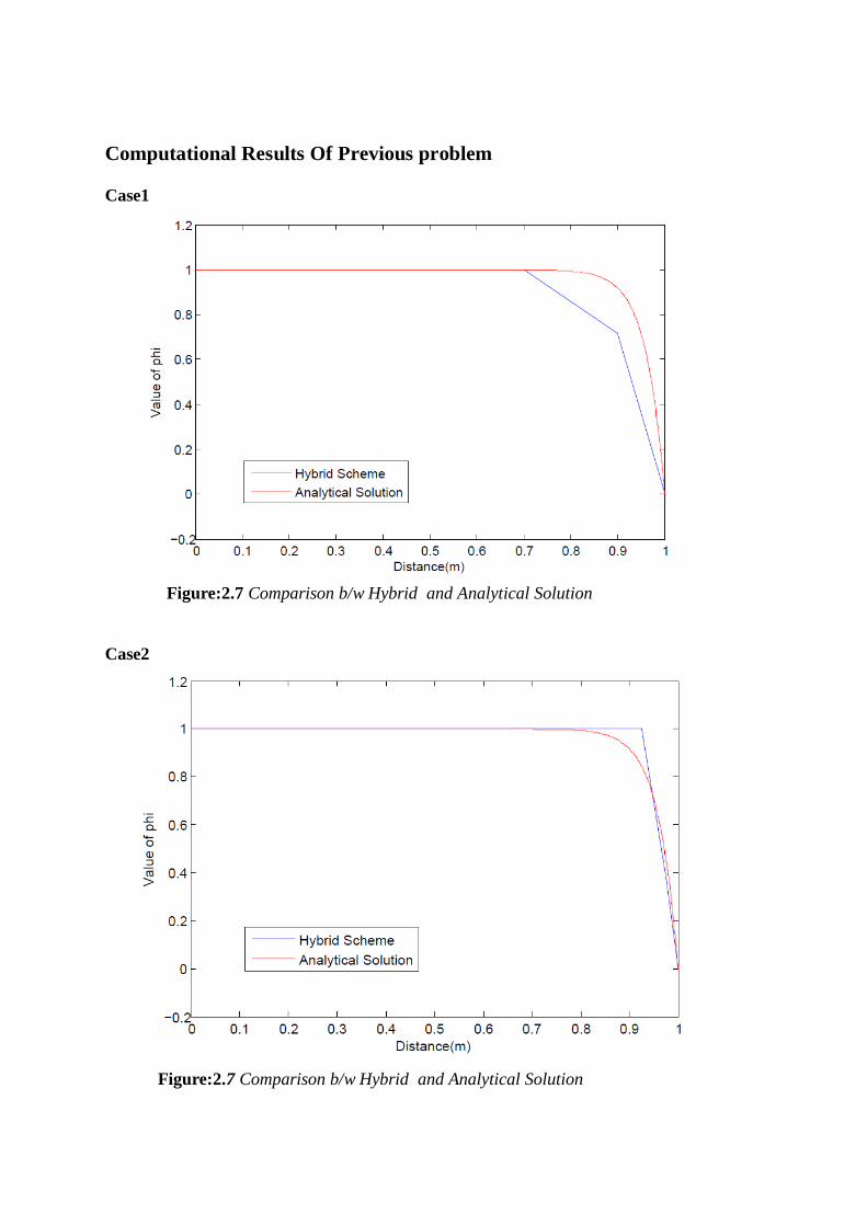
Computational Results Of Previous problem

Case1

Figure:2.7 Comparison b/w Hybrid and Analytical Solution

Case2

Figure:2.7 Comparison b/w Hybrid and Analytical Solution

27

Chapter 3

Concept of Stream-Vorticity Method

This chapter deals with the solution of vorticity, stream function and velocity fields in a laminar

incompressible flow. Navier Stokes equations are used to calculate the solution of equations.

First we will understand the terms vorticity , stream function.

3.1 Streamfunction

The streamfunction represents the two dimensional position representation flow which can be

utilized to calculate the stream lines or the trajectories of the steady state flow. The first

derivative of the stream function give the fluild parcels‟s velocity and second derivative gives

the accelerations. A continuous interconnected stream function gives the

stereamlines for a given snapshot in time. Understanding the location of streamlines is critical in

studying the flow pattern for engineering application. The streamfunction for a given domain

can be solved by the streamfunction equation for one instance in time if the initial position and

magnitude of vorticity is known.

3.2 Vorticity

Vorticity is a physical quantity in fluid dynamics in general for a fluid parcel gives a measure of

its localized rotation. Numerically vorticity is defined as the divergence of the velocity field

( ×V). If the vorticity is known everywhere in the flow the stream function(and hence the

velocity components) is determined by solving a Poisson equation.

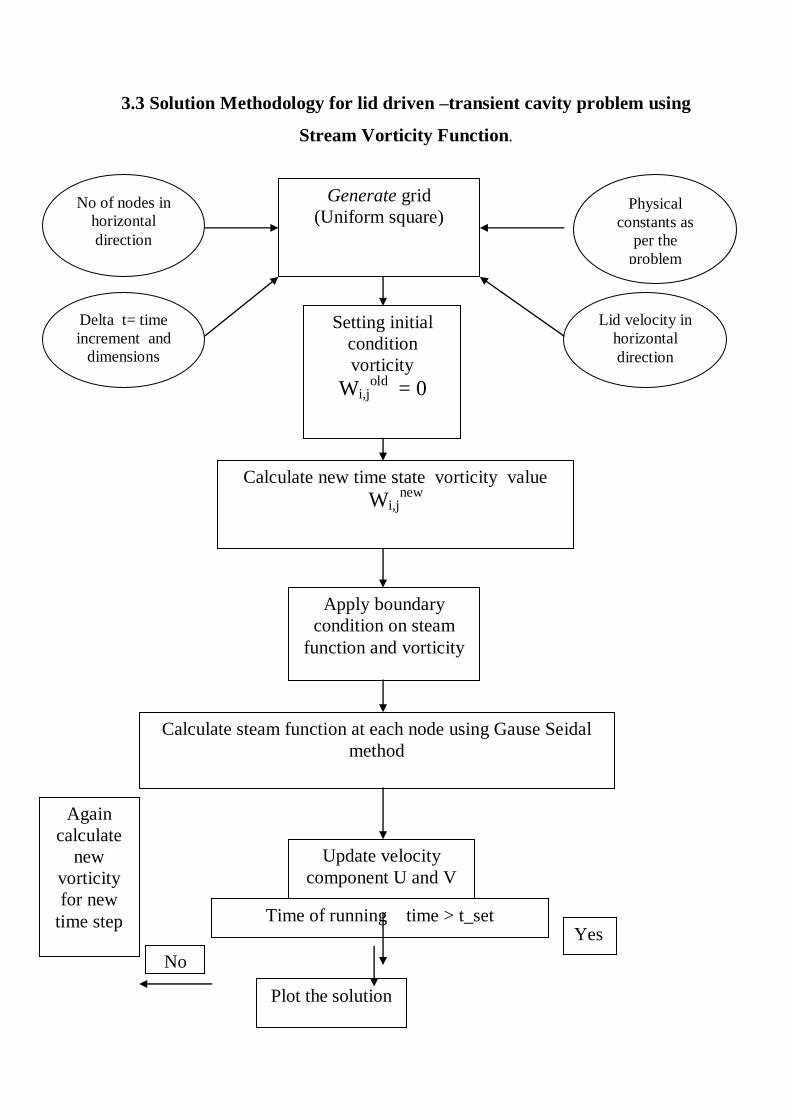
3.3 Solution Methodology for lid driven –transient cavity problem using

Stream Vorticity Function.

Generate grid

(Uniform square)

No of nodes in

horizontal

direction

Delta t= time

increment and

dimensions

And

Physical

constants as

per the

problem

Lid velocity in

horizontal

direction

Setting initial

condition

vorticity

Wi,jold

= 0

Calculate new time state vorticity value

Wi,jnew

Apply boundary

condition on steam

function and vorticity

Calculate steam function at each node using Gause Seidal

method

Update velocity

component U and V

Time of running time > t_set

Plot the solution

Again

calculate

new

vorticity

for new

time step

No

Yes

29

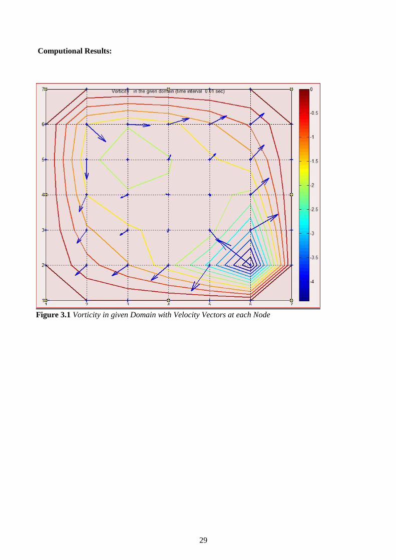
Computional Results:

Figure 3.1 Vorticity in given Domain with Velocity Vectors at each Node

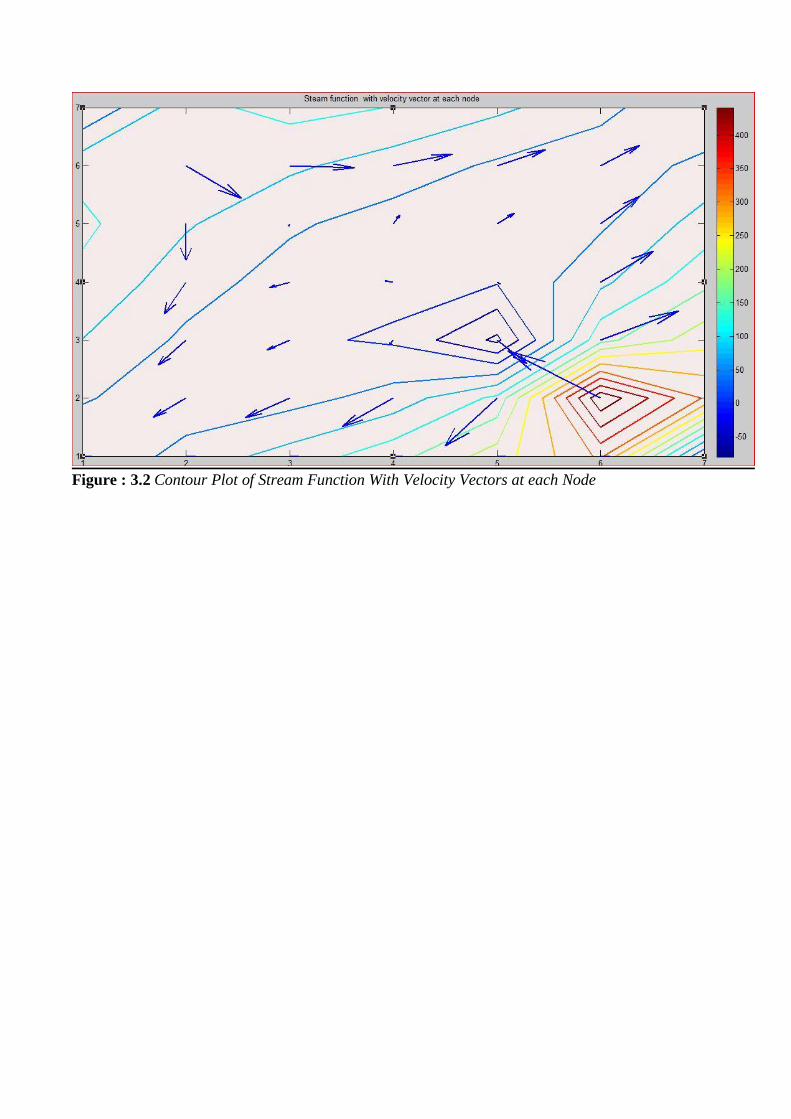
Figure : 3.2 Contour Plot of Stream Function With Velocity Vectors at each Node

31

Chapter 4

A Generalized Form Of Advection-Diffusion Equation

So for we have discussed about various scheme for solving advection-diffusion

equation, which directly depends on peclet number (p). In this section we will develop such a

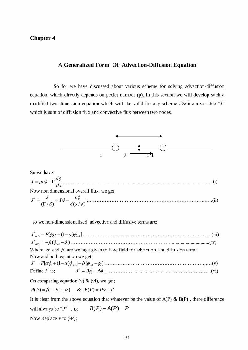
modified two dimension equation which will be valid for any scheme .Define a variable “J”

which is sum of diffusion flux and convective flux between two nodes.

i J i+1

So we have:

dJ u

dx

………………………………………………………………………….…...(i)

Now non dimensional overall flux, we get;

*

( / ) ( / )

J dJ P

d x

;……………………………………………………………..….(ii)

so we non-dimensionalized advective and diffusive terms are;

*

1[ (1 ) ]adv i iJ P …………………………………………………………………...(iii) *

1( )diff i iJ ……………………………………………………...............................(iv)

Where and are weitage given to flow field for advection and diffusion term;

Now add both equation we get; *

1 1[ (1 ) ] ( )i i i iJ P ……………………………………………………,,…(v)

Define *J as; *

1i iJ B A ……………………………………………………...(vi)

On comparing equation (v) & (vi), we get;

( ) (1 )A P P & ( )B P P

It is clear from the above equation that whatever be the value of A(P) & B(P) , there difference

will always be “P” , i,e ( ) ( )B P A P P

Now Replace P to (-P);

( ) ( )B P A P P

i.e on comparing both equation we get;

( ) ( )B P A P & ( ) ( )B P A P

To obtain Relation between ( )A P & (| |)A P

When P > 0, ( ) (| |)A P A P …………(a)

We have ; ( ) ( )B P A P P ; because ( ) ( )B P A P

So we get , ( ) ( )A P A P P …………………………….(b)

On combining equation (a) & (b), we for P<0 ;

we get; ( ) (| |)A P A P P , so in general we get;

( ) (| |) max( ,0)A P A P P

Similarily , ( ) (| |) max( ,0)B P A P P p

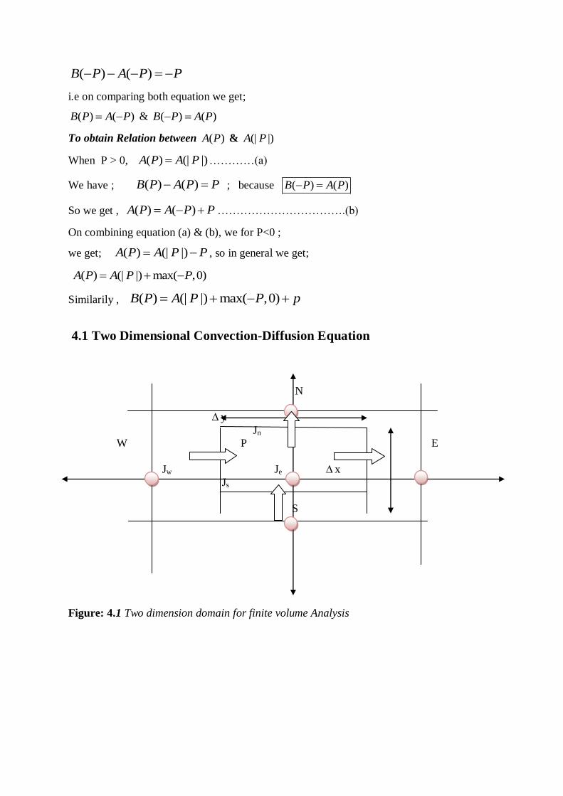
4.1 Two Dimensional Convection-Diffusion Equation

N

y

Jn

W P E

Jw Je x

Js

S

Figure: 4.1 Two dimension domain for finite volume Analysis

33

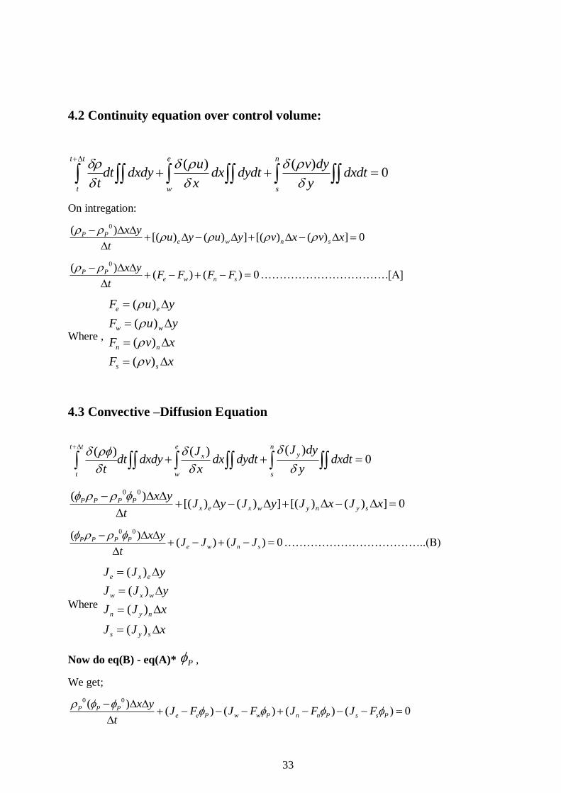
4.2 Continuity equation over control volume:

( ) ( )0

t t e n

t w s

u v dydt dxdy dx dydt dxdt

t x y

On intregation:

0( )[( ) ( ) ] [( ) ( ) ] 0P P

e w n s

x yu y u y v x v x

t

0( )( ) ( ) 0P P

e w n s

x yF F F F

t

…………………………….[A]

Where ,

( )

( )

( )

( )

e e

w w

n n

s s

F u y

F u y

F v x

F v x

4.3 Convective –Diffusion Equation

( )( )( )0

t t e nyx

t w s

J dyJdt dxdy dx dydt dxdt

t x y

0 0( )[( ) ( ) ] [( ) ( ) ] 0P P P P

x e x w y n y s

x yJ y J y J x J x

t

0 0( )( ) ( ) 0P P P P

e w n s

x yJ J J J

t

………………………………..(B)

Where

( )

( )

( )

( )

e x e

w x w

n y n

s y s

J J y

J J y

J J x

J J x

Now do eq(B) - eq(A)* P ,

We get;

0 0( )( ) ( ) ( ) ( ) 0P P P

e e P w w P n n P s s P

x yJ F J F J F J F

t

Where ;

( ) { } [ ] [ ]( / )

e e P x e e P e e e P e e e e e P

e e e

u d dJ F J y F D y F D P F

D D dx d x x

( ) [ ( ) ( ) ] [ ( ) ( ) ]e e P e e P e E e P e e P e P e E e PJ F D B P A P F D A P P A P F

Finally we get,

( ) [ ( ) ( ) ] ( )e e P e e P e E E P EJ F D A P A P a

Similarily , ( ) ( )w w P w w PJ F a

Now assemble all term, we get; 0 0

P P E E W W N N S S P Pa a a a a a

Where 0

0

0 0

0 0

( ) ( ( )) max( ,0)

( ) ( ( )) max( ,0)

( ) ( ( )) max( ,0)

( ) ( ( )) max( ,0)

( )

E e e e e

W w w w w

N n n n n

S s s s s

PP

P P

P E W N S P

a D A P A abs P P

a D B P A abs P P

a D A P A abs P P

a D B P A abs P P

x ya

t

b a

a a a a a a

Here we have calculated flow field at all nodes.

35

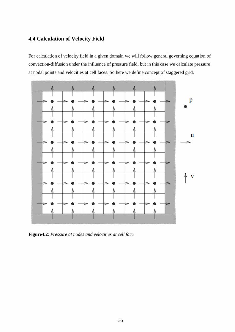
4.4 Calculation of Velocity Field

For calculation of velocity field in a given domain we will follow general governing equation of

convection-diffusion under the influence of pressure field, but in this case we calculate pressure

at nodal points and velocities at cell faces. So here we define concept of staggered grid.

Figure4.2: Pressure at nodes and velocities at cell face

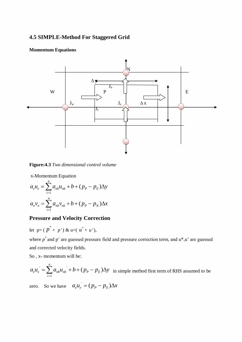
4.5 SIMPLE-Method For Staggered Grid

Momentum Equations

N

y

Jn

W P E

Jw Je x

Js

S

Figure:4.3 Two dimensional control volume

x-Momentum Equation

1

1

( )

( )

n

e e nb nb P E

i

n

n n nb nb P N

i

a u a u b p p y

a v a v b p p x

Pressure and Velocity Correction

let p= (*p + 'p ) & u=(

*u + 'u ),

where p* and p‟ are guessed pressure field and pressure correction term, and u*,u‟ are guessed

and corrected velocity fields.

So , x- momentum will be:

' '

1

( )n

e e nb nb P E

i

a u a u b p p y

in simple method first term of RHS assumed to be

zero. So we have ' ( )e e P Ea u p p x

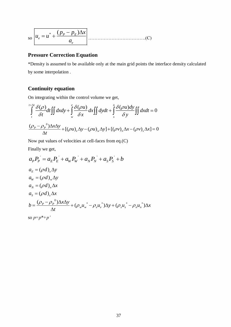
37

so * ( )P E

e

e

p p xu u

a

……………………………….(C)

Pressure Correction Equation

*Density is assumed to be available only at the main grid points the interface density calculated

by some interpolation .

Continuity equation

On integrating within the control volume we get,

( ) ( ) ( )0

t t e n

t w s

u u dydt dxdy dx dydt dxdt

t x y

0( )[( ) ( ) ] [( ) ( ) ] 0P P

e w n s

x yu y u y v x v x

t

Now put values of velocities at cell-faces from eq.(C)

Finally we get,

' ' ' ' '

P P E E W W N N S Sa P a P a P a P a P b

0* * * *

( )

( )

( )

( )

( )( ) ( )

E e

W w

N n

S s

P Pw w e e s s n n

a d y

a d y

a d x

a d x

x yb u u y u u x

t

so p=p*+p’

4.6 Solution Methodology OF “SIMPLE”-Method

1. Guess the pressure field *p .

2. Solve the momentum equations, such as given below to obtain *, *, *u v w

3. Solve the pequation ' ' ' ' '

P P E E W W N N S Sa P a P a P a P a P b

4. Calculate p from given equation by adding p to *p .

5. Calculate u, v, and w from their starred values using the velocity correction formulas

6. Solve the discretization equation for other 's (such as temperature, concentration, and

turbulence quantities ) if they influence the flow field through fluid properties, source terms,

etc.(If a particular does not influence the flow field, it is better to calculate it after a

converged solution for the flow field has been obtained.)

7. Treat the corrected pressure p as a new guessed pressure *p , return to step 2, and repeat the

whole procedure until a converged solution is obtained.

39

4.7 Adaptive Grid In Two Dimensional Boundary Layer

In general, the governing equation for steady two-dimensional boundary layer phenomena

can be written as:

[ ]( ) ( )

rur vr y

rSx y y

In case of momentum conservation ɸ = u (streamwise velocity), Γɸ = µ (viscosity), Sɸ =

p

x

+ Bx.

Above partial differential equation is parabolic in nature. It can be shown using comparing

it with general 2 dimensional partial differential equation. 2 * 0b a c . (Where b=a=0, c=-

1). Hence marching solution procedure can be followed from upstream to downstream.

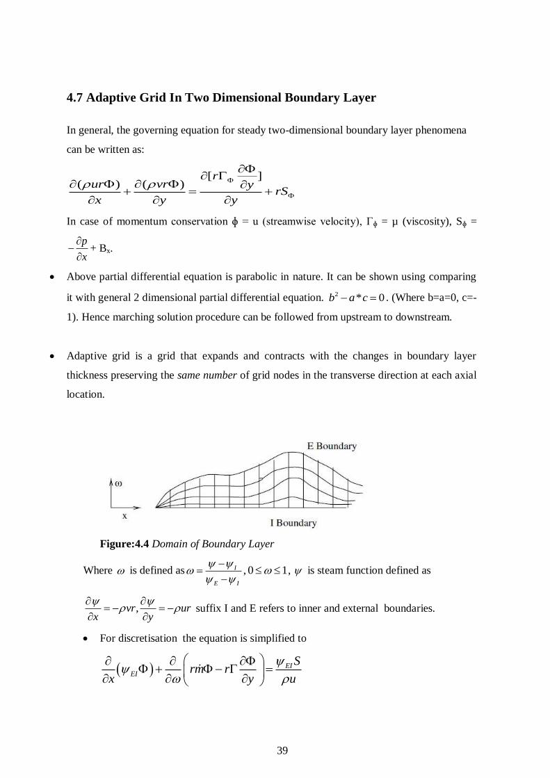
Adaptive grid is a grid that expands and contracts with the changes in boundary layer

thickness preserving the same number of grid nodes in the transverse direction at each axial

location.

Figure:4.4 Domain of Boundary Layer

Where is defined as I

E I

, 0 1 , is steam function defined as

,vr urx y

suffix I and E refers to inner and external boundaries.

For discretisation the equation is simplified to

EIEI

Srm r

x y u

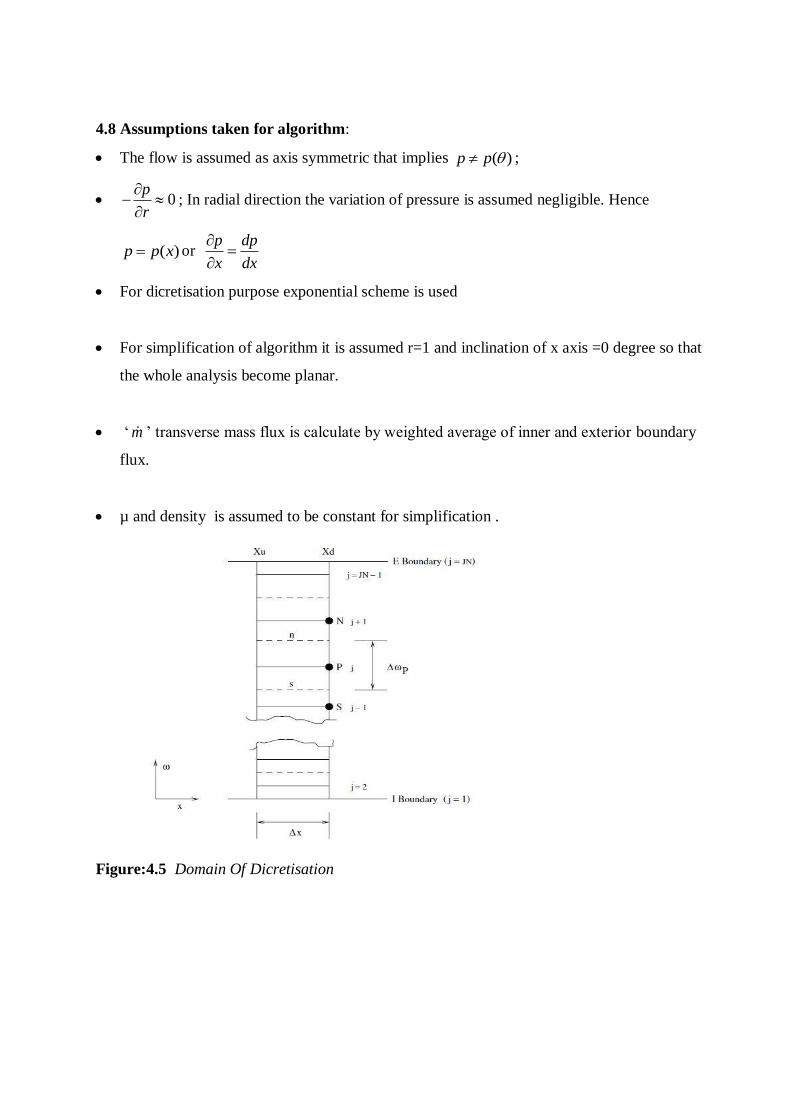
4.8 Assumptions taken for algorithm:

The flow is assumed as axis symmetric that implies ( )p p ;

0p

r

; In radial direction the variation of pressure is assumed negligible. Hence

( )p p x or p dp

x dx

For dicretisation purpose exponential scheme is used

For simplification of algorithm it is assumed r=1 and inclination of x axis =0 degree so that

the whole analysis become planar.

„ m ‟ transverse mass flux is calculate by weighted average of inner and exterior boundary

flux.

µ and density is assumed to be constant for simplification .

Figure:4.5 Domain Of Dicretisation

41

4.9 Algorithm

1. Decide grid pattern according to the given geometry ,x y

2. Specify initial condition (steam function at first axial point x0 start line, 0 0( )x x )

3. Using *

0 , ,u y calculate j using

1 1 1 1 10.5( )*( )j j j j j j j j j jr u r u y y

4. Specify boundary condition in terms of ,E I

5. Using boundary condition ,E I and j , find

j , using definition , I

E I

6. Guess initial velocity and pressure distribution * * *, ,u v p in above specified grid at each

nodal point.

7. Find the transverse mass flux m

(1 )* * ,j j I j Em m m

Where ( )I Im v and ( )E Em v

8. Follow the discretised equation „d‟ denotes downstream and „u‟ denotes upstream values

exp

' 'exp 1 exp 1

,

d d d u

P N S P

m n s s cs

cn cs

u

EI

AP AN AS AU S V

r m x r m x PAN AS

P P

AU AP AU AN AS

For plane boundary layer phenomena r=1 for all nodes.

For application of boundary condition the second and next to last node is used.

The specification of the three types of flows mentioned here can be sensed through

appropriate designation of I and E boundaries as free, wall, or symmetry boundaries.

9. Calculate *n

n P N nc n

P N

y y y yP m

and *

s

s S P sc s

S P

y y y yP m

10. For source term

1

( )

u d

j j

j x j

j j

p pS B

x x

, and pV r x y where pr =1 for planar analysis, ( )x jB is

nodal body force distribution

11. Hence all the coefficients are known up to this stage. Using boundary condition at

interior and exterior boundaries velocity at intermediate nodes of upstream line can be

calculated using either matrix inversion or Gauss-Seidal approach.

12. Update old values using new values of velocity. Follow the marching procedure for

known initial condition at 0x x , calculate velocity distribution at each x=xj line.

13. Check for convergence in u and v values and perform iteration repeatedly until

convergence achieved.

43

Chapter 5

Implementation of TDMA (Tri-diagonal Matrix Algorithm) in solving linear

equations

5.1 Introduction about TDMA

In numerical linear algebra the tri-diagonal matrix algorithm (TDMA), also known as

the Thomas algorithm (named after Llewellyn Thomas), is a simplified form of Gaussian

elimination that can be used to solve tri-diagonal system of linear equations of type Ax=B.

5.2 Implementation on a sample problem

The algorithm for solving „Ax=B‟ type linear equations in which „A‟ is necessarily tri-

diagonal matrix is based on forward elimination and back substitution using recurrence

relationship . [Ref 1]. In case of one dimensional problem the coefficient matrix „A‟ is tri-

diagonal in nature , hence it is directly solved for unknowns. However in case of two or

three or higher dimensional problems the coefficient matrix „A‟ is not necessarily tri-

diagonal. So one have to apply TDMA line by line and sweep in any particular direction to

find unknowns over a given domain. This must be a repetitive procedure using iteration

until a converged solution is obtained with minimum of nodal RMS (root mean square)

error. The sample problem was taken from [Ref 1]. The aim of problem was to get

unknown temperature on a two dimensional domain. The boundary conditions were given

in the problem. The main aim of solving the sample problem was to get used to solving

linear equations using TDMA. The implementation of TDMA by sweeping line by line can

be used to solve mass and momentum equations over two dimensional domain.

Moreover, in comparison of Gause-Seidel and TDMA ,it was observed clearly that

computation time was less in TDMA .

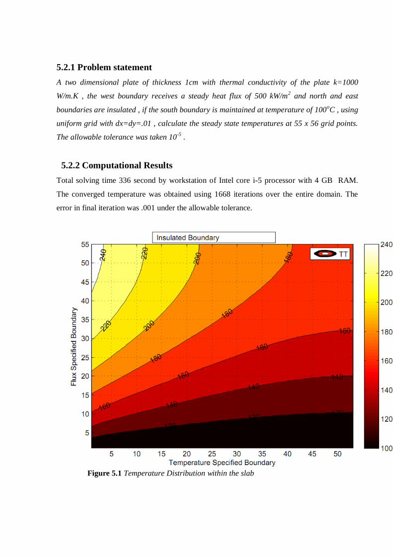
5.2.1 Problem statement

A two dimensional plate of thickness 1cm with thermal conductivity of the plate k=1000

W/m.K , the west boundary receives a steady heat flux of 500 kW/m2 and north and east

boundaries are insulated , if the south boundary is maintained at temperature of 100oC , using

uniform grid with dx=dy=.01 , calculate the steady state temperatures at 55 x 56 grid points.

The allowable tolerance was taken 10-5

.

5.2.2 Computational Results

Total solving time 336 second by workstation of Intel core i-5 processor with 4 GB RAM.

The converged temperature was obtained using 1668 iterations over the entire domain. The

error in final iteration was .001 under the allowable tolerance.

Figure 5.1 Temperature Distribution within the slab

45

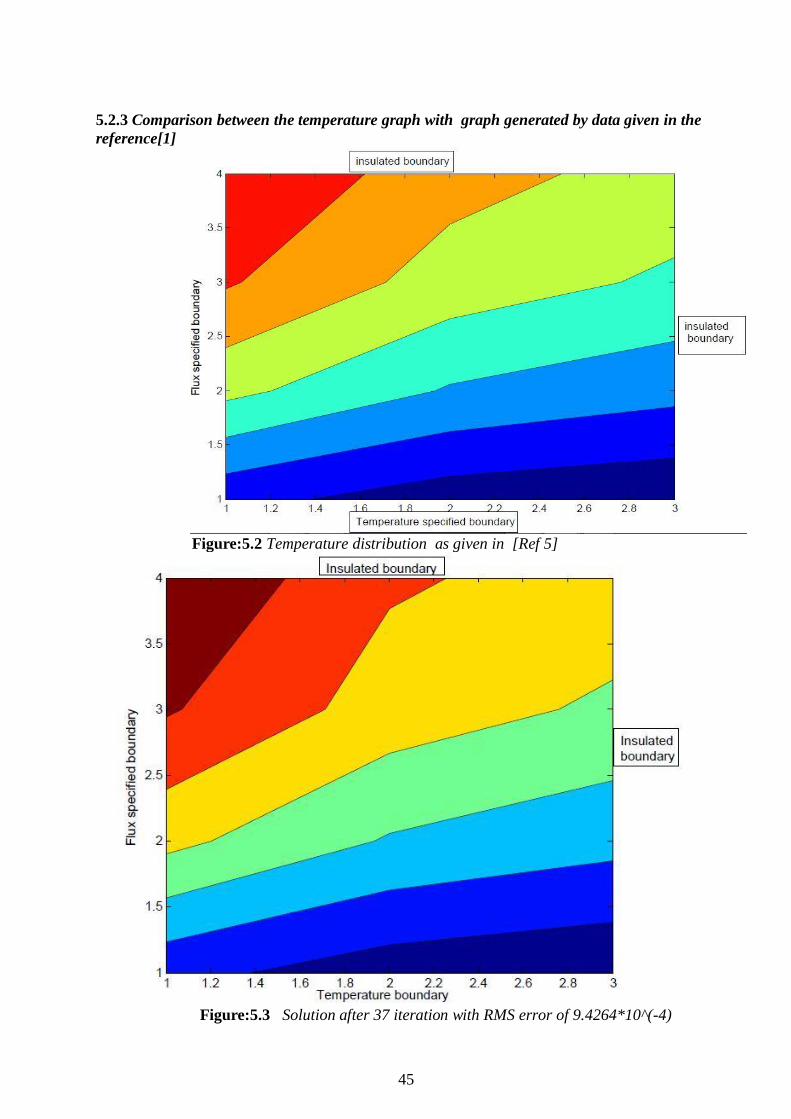
5.2.3 Comparison between the temperature graph with graph generated by data given in the

reference[1]

Figure:5.2 Temperature distribution as given in [Ref 5]

Figure:5.3 Solution after 37 iteration with RMS error of 9.4264*10^(-4)

Chapter 6

Analysis of Lid Driven Cavity Flow

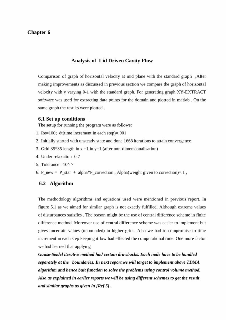
Comparison of graph of horizontal velocity at mid plane with the standard graph ,After

making improvements as discussed in previous section we compare the graph of horizontal

velocity with y varying 0-1 with the standard graph. For generating graph XY-EXTRACT

software was used for extracting data points for the domain and plotted in matlab . On the

same graph the results were plotted .

6.1 Set up conditions

The setup for running the program were as follows:

1. Re=100; dt(time increment in each step)=.001

2. Initially started with unsteady state and done 1668 iterations to attain convergence

3. Grid 35*35 length in x =1,in y=1,(after non-dimensionalisation)

4. Under relaxation=0.7

5. Tolerance= 10^-7

6. P_new = P_star + alpha*P_correction , Alpha(weight given to correction)=.1 ,

6.2 Algorithm

The methodology algorithms and equations used were mentioned in previous report. In

figure 5.1 as we aimed for similar graph is not exactly fulfilled. Although extreme values

of disturbances satisfies . The reason might be the use of central difference scheme in finite

difference method. Moreover use of central difference scheme was easier to implement but

gives uncertain values (unbounded) in higher grids. Also we had to compromise to time

increment in each step keeping it low had effected the computational time. One more factor

we had learned that applying

Gause-Seidel iterative method had certain drawbacks. Each node have to be handled

separately at the boundaries. In next report we will target to implement above TDMA

algorithm and hence buit function to solve the problems using control volume method.

Also as explained in earlier reports we will be using different schemes to get the result

and similar graphs as given in [Ref 5] .

47

6.3 Result

Figure:6.1 Comaparison b/w our results and standerd result

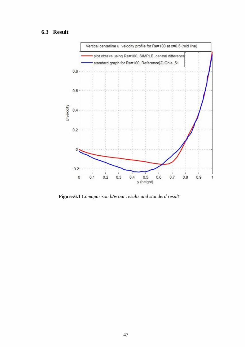
6.4 SIMPLE-Method for Collocated Grid

So far we have seen that SIMPLE-staggered grid method enjoyed considerable success

particularly when Cartesian grids were employed , but the procedure was found to be

inconvenient when curvilinear or adaptive grids were to be employed to compute over more

complex domains . It was found that if the pressure correction equation as derived for staggered

grids was used to predict pressure on collocated grids the resulting pressure distribution showed

zig-zagness. Here we shall describe the method proposed by Date that elegantly eliminates the

problem of zigzag pressure prediction.

Figure:6.2 Domain of discretisation for Collocated grid

49

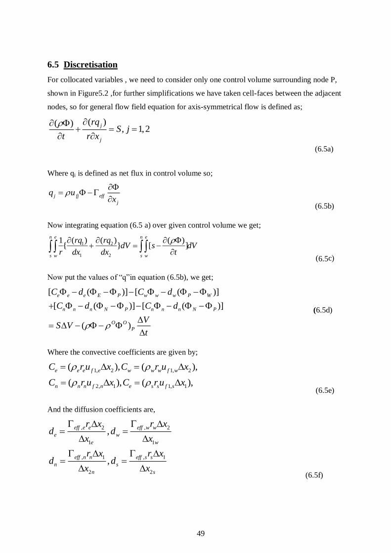
6.5 Discretisation

For collocated variables , we need to consider only one control volume surrounding node P,

shown in Figure5.2 ,for further simplifications we have taken cell-faces between the adjacent

nodes, so for general flow field equation for axis-symmetrical flow is defined as;

( )( ), 1,2

j

j

rqS j

t r x

(6.5a)

Where qi is defined as net flux in control volume so;

j fj eff

j

q ux

(6.5b)

Now integrating equation (6.5 a) over given control volume we get;

1 2

1 2

( ) ( )1 ( ){ } [ ]

n e n e

s w s w

rq rqdV s dV

r dx dx t

(6.5c)

Now put the values of “q”in equation (6.5b), we get;

[ ( )] [ ( )]

[ ( )] [ ( )]

( )

e e e E P w w w P W

n n n N P n n n N P

O O

P

C d C d

C d C d

VS V

t

(6.5d)

Where the convective coefficients are given by;

1, 2 1, 2

2, 1 1, 1

( ), ( ),

( ), ( ),

e e e f e w w w f w

n n n f n e s s f s

C r u x C r u x

C r u x C r u x

(6.5e)

And the diffusion coefficients are,

, 2 , 2

1 1

, 1 , 1

2 2

,

,

eff e e eff w w

e w

e w

eff n n eff s s

n s

n s

r x r xd d

x x

r x r xd d

x x

(6.5f)

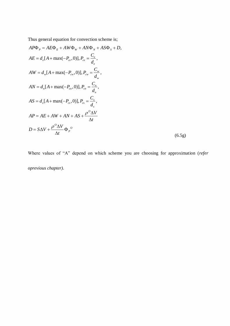
Thus general equation for convection scheme is;

,

[ max( ,0)], ,

[ max( ,0)], ,

[ max( ,0)], ,

[ max( ,0)], ,

P E W N S

ee ce ce

e

ww cw cw

w

nn cn cn

n

ss cs cs

s

O

OO

P

AP AE AW AN AS D

CAE d A P P

d

CAW d A P P

d

CAN d A P P

d

CAS d A P P

d

VAP AE AW AN AS

t

VD S V

t

(6.5g)

Where values of “A” depend on which scheme you are choosing for approximation (refer

oprevious chapter).

51

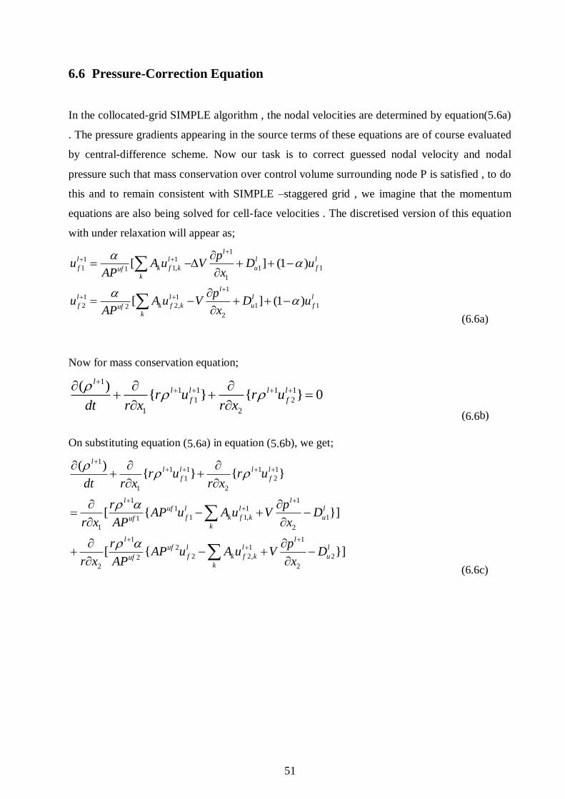
6.6 Pressure-Correction Equation

In the collocated-grid SIMPLE algorithm , the nodal velocities are determined by equation(5.6a)

. The pressure gradients appearing in the source terms of these equations are of course evaluated

by central-difference scheme. Now our task is to correct guessed nodal velocity and nodal

pressure such that mass conservation over control volume surrounding node P is satisfied , to do

this and to remain consistent with SIMPLE –staggered grid , we imagine that the momentum

equations are also being solved for cell-face velocities . The discretised version of this equation

with under relaxation will appear as;

11 1

1 1, 1 11

1

11 1

2 2, 1 12

2

[ ] (1 )

[ ] (1 )

ll l l l

f k f k u fufk

ll l l l

f k f k u fufk

pu A u V D u

AP x

pu A u V D u

AP x

(6.6a)

Now for mass conservation equation;

11 1 1 1

1 2

1 2

( ){ } { } 0

ll l l l

f fr u r udt r x r x

(6.6b)

On substituting equation (5.6a) in equation (5.6b), we get;

11 1 1 1

1 2

1 2

1 11 1

1 1, 11

1 2

1 12 1

2 2, 22

2 2

( ){ } { }

[ { }]

[ { }]

ll l l l

f f

l luf l l l

f k f k uufk

l luf l l l

f k f k uufk

r u r udt r x r x

r pAP u A u V D

r x AP x

r pAP u A u V D

r x AP x

(6.6c)

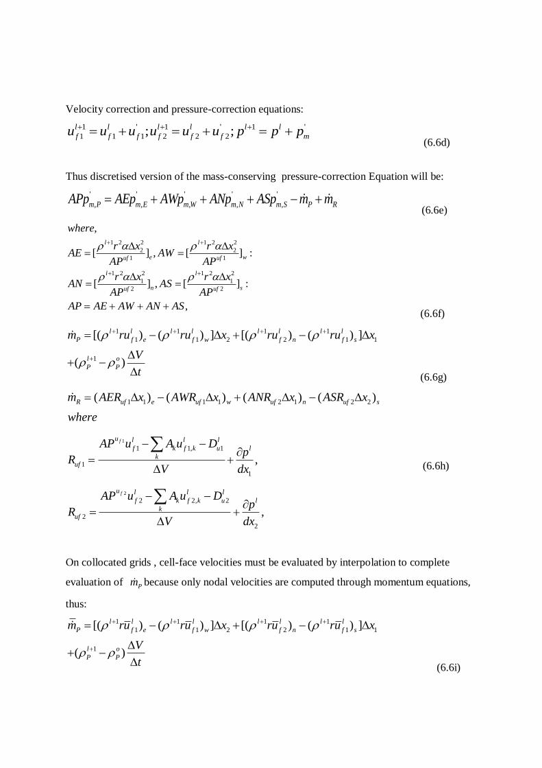
Velocity correction and pressure-correction equations:

1 ' 1 ' 1 '

1 1 1 2 2 2; ;l l l l l l

f f f f f f mu u u u u u p p p (6.6d)

Thus discretised version of the mass-conserving pressure-correction Equation will be:

' ' ' ' '

, , , , ,m P m E m W m N m S P RAPp AEp AWp ANp ASp m m (6.6e)

1 2 2 1 2 2

2 2

1 1

1 2 2 1 2 2

1 1

2 2

,

[ ] , [ ] :

[ ] , [ ] :

,

l l

e wuf uf

l l

n suf uf

where

r x r xAE AW

AP AP

r x r xAN AS

AP AP

AP AE AW AN AS

(6.6f)

1 1 1 1

1 1 2 2 1 1

1

[( ) ( ) ] [( ) ( ) ]

( )

l l l l l l l l

P f e f w f n f s

l o

P P

m ru ru x ru ru x

V

t

(6.6g)

1

2

1 1 1 1 2 1 2 2

1 1, 1

1

1

2 2, 2

2

2

( ) ( ) ( ) ( )

,

,

f

f

R uf e uf w uf n uf s

u l l l

lf k f k u

kuf

u l l l

lf k f k u

kuf

m AER x AWR x ANR x ASR x

where

AP u A u Dp

RV dx

AP u A u Dp

RV dx

(6.6h)

On collocated grids , cell-face velocities must be evaluated by interpolation to complete

evaluation of Pm because only nodal velocities are computed through momentum equations,

thus:

1 1 1 1

1 1 2 2 1 1

1

[( ) ( ) ] [( ) ( ) ]

( )

l l l l l l l l

P f e f w f n f s

l o

P P

m ru ru x ru ru x

V

t

(6.6i)

53

Now for evaluating cell-faces velocities, we use multidimensional averaging rather than simple

one dimensional averaging, thus:

2, 1, 2, 1,

1, 1, 1,

2, 2,

1, 1, 1, 1, 1,

1, 1, 1, 1, 1,

1 1[ ( ) ]

2 2

1( ),

4

1( ),

4

l l

n se s nel l l

e P E

n s

l l l l l

se P E S SE

l l l l l

ne P E N NE

x u x uu u u

x x

u u u u u

u u u u u

(5.6 j)

1

1

1 1, 1

1,

1

1 1, 1

1,

1

( ) ( )

( ) ( )

f

f

u l l l

lf k f k u

kuf e e e

u l l l

lf k f k u

ke uf e e

AP u A u Dp

R avgV dx

AP u A u Dp

avg RV dx

(6.6k)

Finally we get: ' ' ' '

1 1 2 2

1 1 2 2

( ) ( ) ( ) ( )sm sm sm smR e w n s

p p p pm AE x AW x AN x AS x

dx dx dx dx

(6.6l)

1, 1,

1,

1, 1,

1, 2,

1, 1,

1,

1, 1,

2, 2,

2,

2, 2,

1, 2,

1( ),

2

,

,

1( ),

2

w E e W

x P

w e

P x P x P

e EE ee P

x E

e ee

s NE n SE

x E

s n

E x E x E

x p x pp

x x

p p p

x p x pp

x x

x p x pp

x x

p p p

' ' '

m smp p p (6.6m)

6.7 Overall Calculation Procedure

1. At a given time step, guess the pressure field and velocity field at nodes.

2. Solve the momentumequation using equation (6.5g) with problem dependent boundary

condition.

3. Solve equation (6.6e), which yield total pressure-correction field.

4. Recover the mass-conserving pressure, thus

' ' ' '

, , , , , , , ,

1( )

2

l l

m i j i j sm i j i j i j i jp p p p p p

5. Correct the pressure and velocity fields according to:

1 '

, , , ,

1 ' '21, , 1, , , , 1/2, , 1/2,1

1 ' '12, , 2, , , , , 1/2 , , 1/22

{ } ( ),

{ } ( ),

l l

i j i j m i j

l l

i j i j i j m i j m i ju

l l

i j i j i j m i j m i ju

p p p

r xu u p p

AP

r xu u p p

AP

6. solve the discretised equations (6.2g) for all other scalar relevant to the problem at hand.

7. Check convergence through evaluation of residuals for momentum.

8. If the convergence criterion is not satisfied treat

1 1,l l l lp p And return to step 2.

9.To execute the next time step,set all 1o l and return to step 1.

55

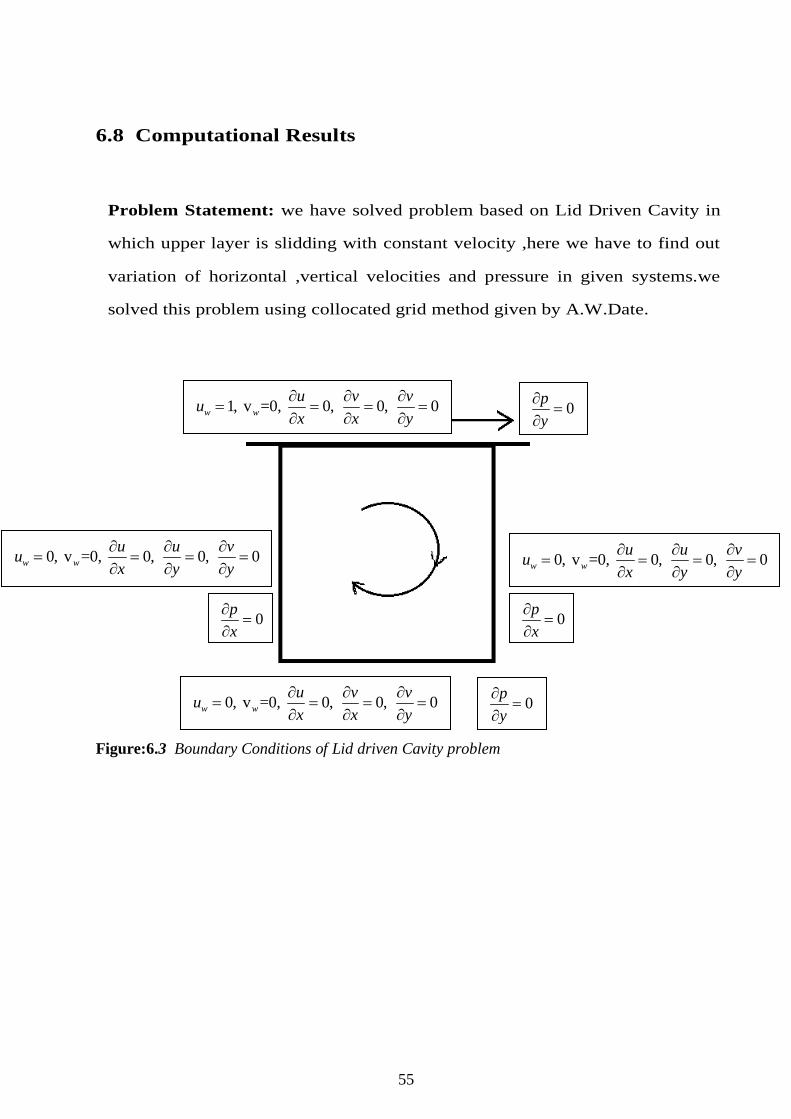
6.8 Computational Results

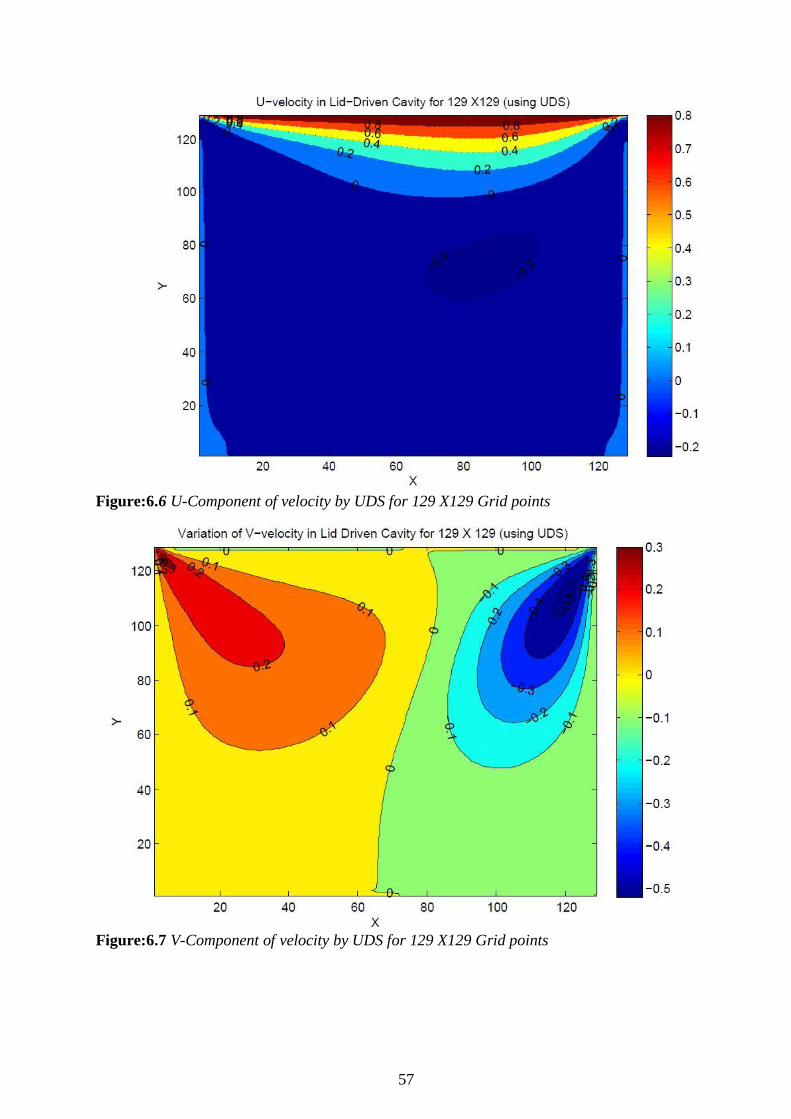
Problem Statement: we have solved problem based on Lid Driven Cavity in

which upper layer is slidding with constant velocity ,here we have to find out

variation of horizontal ,vertical velocities and pressure in given systems.we

solved this problem using collocated grid method given by A.W.Date.

Figure:6.3 Boundary Conditions of Lid driven Cavity problem

1, v =0, 0, 0, 0w w

u v vu

x x y

0, v =0, 0, 0, 0w w

u u vu

x y y

0, v =0, 0, 0, 0w w

u u vu

x y y

0, v =0, 0, 0, 0w w

u v vu

x x y

0p

x

0p

y

0p

y

0p

x

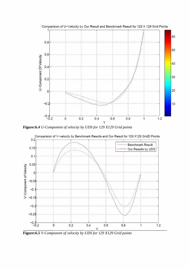
Figure:6.4 U-Component of velocity by UDS for 129 X129 Grid points

Figure:6.5 V-Component of velocity by UDS for 129 X129 Grid points

57

Figure:6.6 U-Component of velocity by UDS for 129 X129 Grid points

Figure:6.7 V-Component of velocity by UDS for 129 X129 Grid points

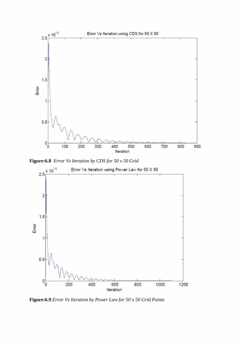
Figure:6.8 Error Vs Iteration by CDS for 50 x 50 Grid

Figure:6.9 Error Vs Iteration by Power Law for 50 x 50 Grid Points

59

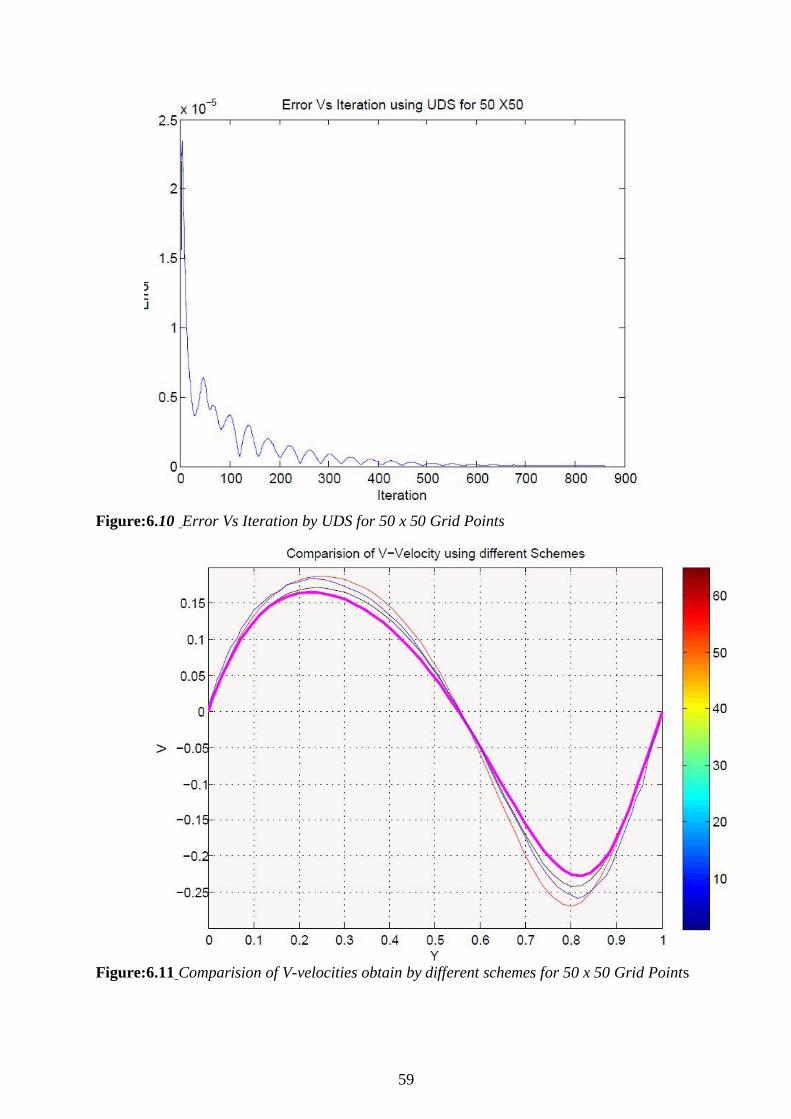
Figure:6.10 Error Vs Iteration by UDS for 50 x 50 Grid Points

Figure:6.11 Comparision of V-velocities obtain by different schemes for 50 x 50 Grid Points

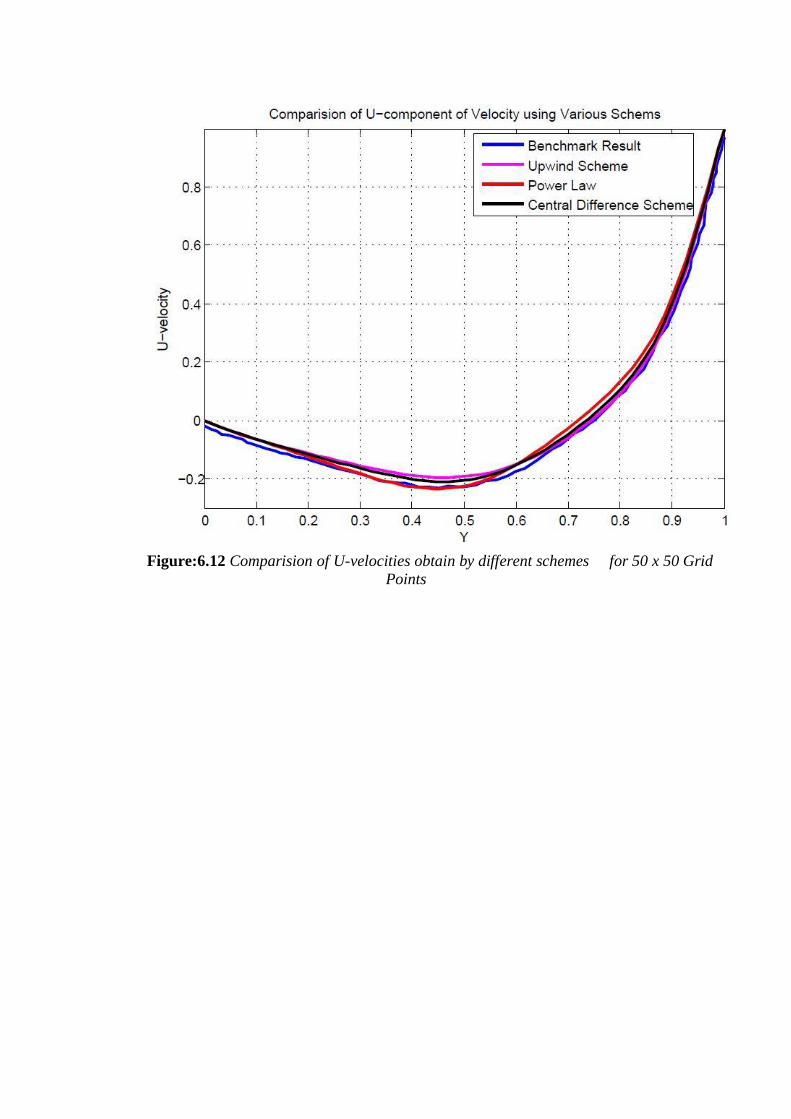
Figure:6.12 Comparision of U-velocities obtain by different schemes for 50 x 50 Grid

Points

61

Chapter 7

Concept Of Adaptive Grid

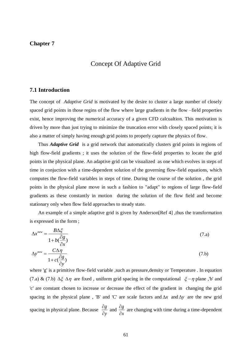
7.1 Introduction

The concept of Adaptive Grid is motivated by the desire to cluster a large number of closely

spaced grid points in those regins of the flow where large gradients in the flow –field properties

exist, hence improving the numerical accuracy of a given CFD calcualtion. This motivation is

driven by more than just trying to minimize the truncation error with closely spaced points; it is

also a matter of simply having enough grid points to properly capture the physics of flow.

Thus Adaptive Grid is a grid network that automatically clusters grid points in regions of

high flow-field gradients ; it uses the solution of the flow-field properties to locate the grid

points in the physical plane. An adaptive grid can be visualized as one which evolves in steps of

time in conjuction with a time-dependent solution of the governing flow-field equations, which

computes the flow-field variables in steps of time. During the course of the solution , the grid

points in the physical plane move in such a fashion to "adapt" to regions of large flow-field

gradients as these constantly in motion during the solution of the flow field and become

stationary only when flow field approaches to steady state.

An example of a simple adaptive grid is given by Anderson[Ref 4] ,thus the transformation

is expressed in the form ;

1 ( )

new Bx

gb

x

(7.a)

1 ( )

new Cy

gc

y

(7.b)

where 'g' is a primitive flow-field variable ,such as pressure,density or Temperature . In equation

(7.a) & (7.b) are fixed , uniform grid spacing in the computational plane ,'b' and

'c' are constant chosen to increase or decrease the effect of the gradient in changing the grid

spacing in the physical plane , 'B' and 'C' are scale factors and x and y are the new grid

spacing in physical plane. Because g

y

and

g

x

are changing with time during a time-dependent

solution of the flow field then clearly x and y change with time ; i.e the grid points moves in

the physical domain,for detailed discussion on it given in [Ref 4].

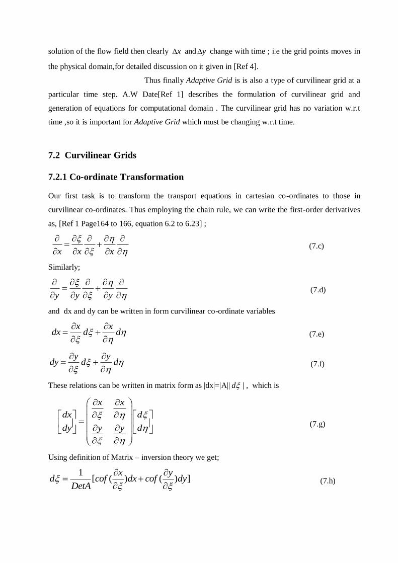
Thus finally Adaptive Grid is is also a type of curvilinear grid at a

particular time step. A.W Date[Ref 1] describes the formulation of curvilinear grid and

generation of equations for computational domain . The curvilinear grid has no variation w.r.t

time ,so it is important for Adaptive Grid which must be changing w.r.t time.

7.2 Curvilinear Grids

7.2.1 Co-ordinate Transformation

Our first task is to transform the transport equations in cartesian co-ordinates to those in

curvilinear co-ordinates. Thus employing the chain rule, we can write the first-order derivatives

as, [Ref 1 Page164 to 166, equation 6.2 to 6.23] ;

        x x x

(7.c)

Similarly;

y y y

(7.d)

and dx and dy can be written in form curvilinear co-ordinate variables

x x

dx d d

(7.e)

y ydy d d

(7.f)

These relations can be written in matrix form as |dx|=|A|| d | , which is

x x

dx d

dy y y d

(7.g)

Using definition of Matrix – inversion theory we get;

1[ ( ) ( ) ]

x yd cof dx cof dy

DetA

(7.h)

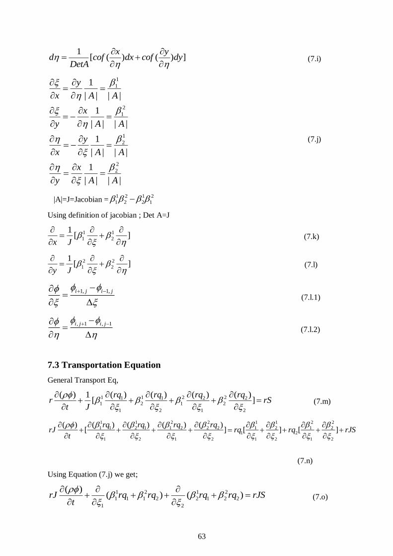
63

1[ ( ) ( ) ]

x yd cof dx cof dy

DetA

(7.i)

1

1

2

1

1

2

2

2

1

| | | |

1

| | | |

1

| | | |

1

| | | |

y

x A A

x

y A A

y

x A A

x

y A A

(7.j)

|A|=J=Jacobian =1 2 1 2

1 2 2 1

Using definition of jacobian ; Det A=J

1 1

1 2

1[ ]

x J

(7.k)

2 2

1 2

1[ ]

y J

(7.l)

1, 1,i j i j

(7.l.1)

, 1 , 1i j i j

(7.l.2)

7.3 Transportation Equation

General Transport Eq,

1 1 2 21 1 2 21 2 1 2

1 2 1 2

( ) ( ) ( ) ( )( ) 1[ ]

rq rq rq rqr rS

t J

(7.m)

1 1 2 2 1 1 2 2

1 1 2 1 1 2 2 2 1 2 1 21 2

1 2 1 2 1 2 1 2

( ) ( ) ( ) ( )( )[ ] [ ] [ ]

rq rq rq rqrJ rq rq rJS

t

(7.n)

Using Equation (7.j) we get;

1 2 1 2

1 1 1 2 2 1 2 2

1 2

( )( ) ( )rJ rq rq rq rq rJS

t

(7.o)

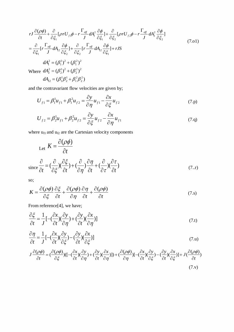
2 2

1 1 2 2

1 1 2 2

12 12

1 2 2 1

( )[ ] [ ]

[ ] [ ]

eff eff

f f

eff eff

rJ rU r dA rU r dAt J J

r dA r dA rJSJ J

(7.o1)

Where

2 1 2 2 2

1 1 1

2 1 2 2 2

2 2 2

1 1 2 2

12 1 2 1 2

( ) ( )

( ) ( )

( )

dA

dA

dA

and the contravariant flow velocities are given by;

1 2

1 1 1 1 2 1 2f f f f f

y xU u u u u

(7.p)

1 2

2 2 1 2 2 2 1f f f f f

y xU u u u u

(7.q)

where uf1 and uf2 are the Cartesian velocity components

Let

( )K

t

since ( )( ) ( ) ( )( )t t t t

(7..r)

so;

( ) ( ) ( )K

t t t

(7.s)

From reference[4], we have;

1[ ( )( ) ( )( )]

x y y x

t J t t

(7.t)

1[ ( )( ) ( )( )]

x y y x

t J t t

(7.u)

( ) ( ) ( ) ( )( )([ ( )( ) ( )( )]) ( )[ ( )( ) ( )( )] ( )

x y y x x y y xJ J

t t t t t t

(7.v)

65

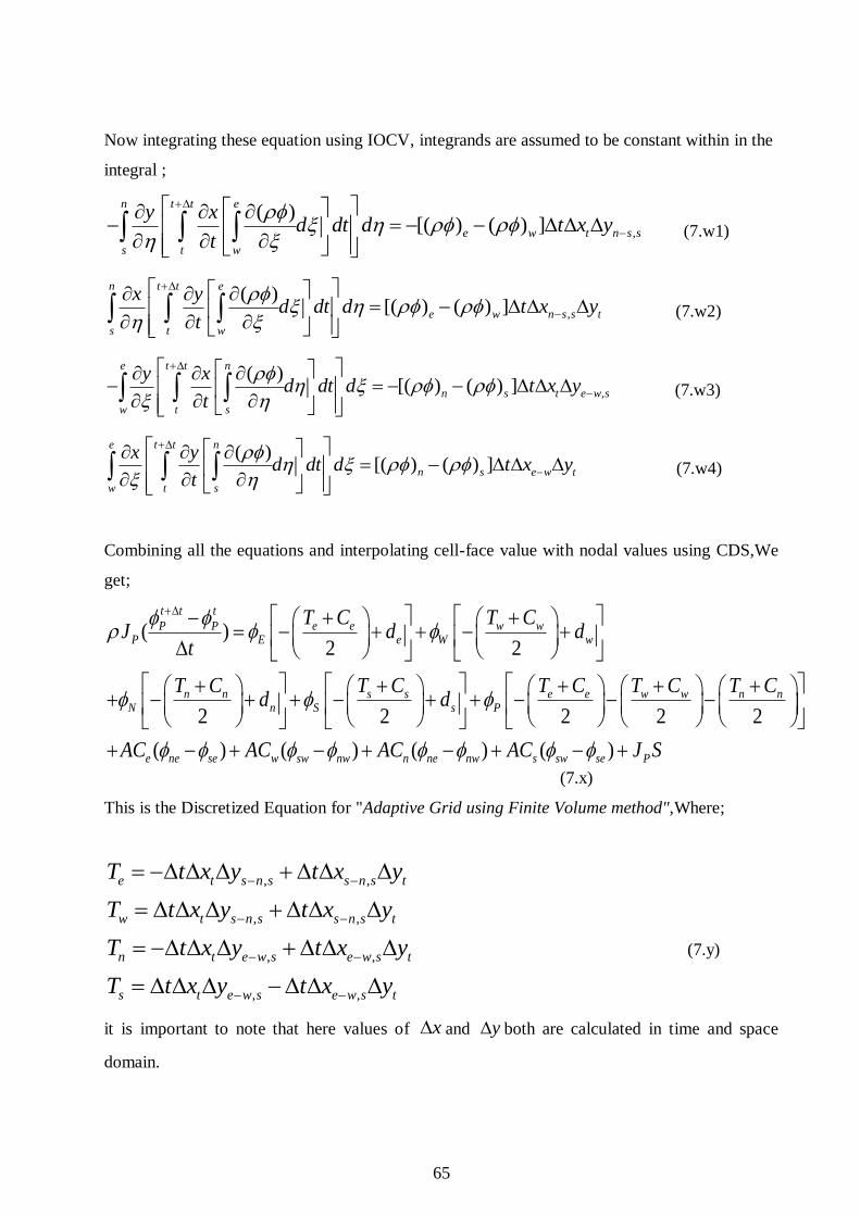
Now integrating these equation using IOCV, integrands are assumed to be constant within in the

integral ;

,

( )[( ) ( ) ]

n t t e

e w t n s s

s t w

y xd dt d t x y

t

(7.w1)

,

( )[( ) ( ) ]

n t t e

e w n s s t

s t w

x yd dt d t x y

t

(7.w2)

,

( )[( ) ( ) ]

e t t n

n s t e w s

w t s

y xd dt d t x y

t

(7.w3)

( )[( ) ( ) ]

e t t n

n s e w t

w t s

x yd dt d t x y

t

(7.w4)

Combining all the equations and interpolating cell-face value with nodal values using CDS,We

get;

( )2 2

2 2 2 2 2

( ) ( ) (

t t t

e e w wP PP E e W w

n n s s e e w w n nN n S s P

e ne se w sw nw n ne

T C T CJ d d

t

T C T C T C T C T Cd d

AC AC AC

) ( )nw s sw se PAC J S

(7.x)

This is the Discretized Equation for "Adaptive Grid using Finite Volume method",Where;

, ,

, ,

, ,

, ,

e t s n s s n s t

w t s n s s n s t

n t e w s e w s t

s t e w s e w s t

T t x y t x y

T t x y t x y

T t x y t x y

T t x y t x y

(7.y)

it is important to note that here values of x and y both are calculated in time and space

domain.

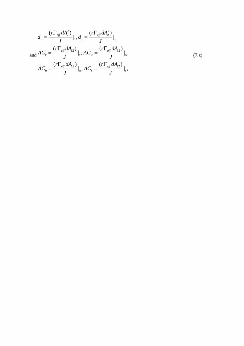
and

2 2

2 2

12 12

12 12

( ) ( )| , |

( ) ( )| , |

( ) ( )| , | ,

eff eff

n n s s

eff eff

e e w w

eff eff

n n s s

r dA r dAd d

J J

r dA r dAAC AC

J J

r dA r dAAC AC

J J

(7.z)

67

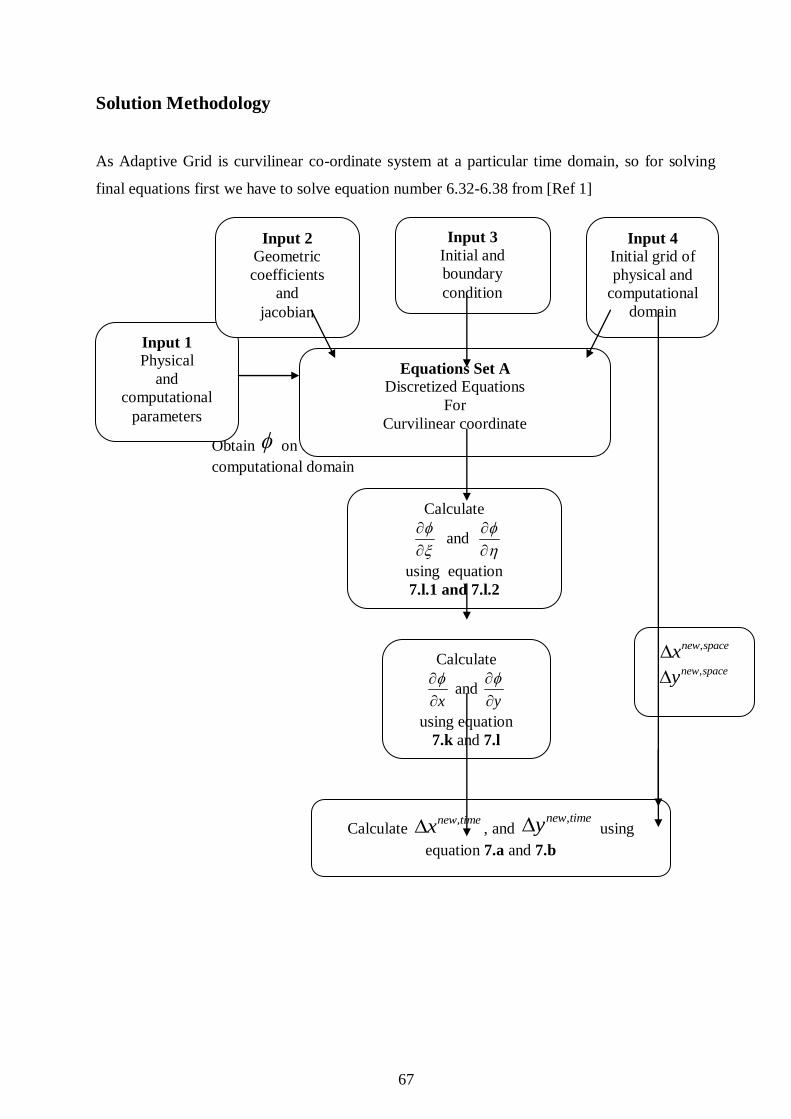
Solution Methodology

As Adaptive Grid is curvilinear co-ordinate system at a particular time domain, so for solving

final equations first we have to solve equation number 6.32-6.38 from [Ref 1]

Obtain on entire

computational domain

Equations Set A

Discretized Equations

For

Curvilinear coordinate

Input 1

Physical

and

computational

parameters

Input 2

Geometric

coefficients

and

jacobian

Input 3

Initial and

boundary

condition

Input 4

Initial grid of

physical and

computational

domain

Calculate

and

using equation

7.l.1 and 7.l.2

---

Calculate

x

and

y

using equation

7.k and 7.l

,new spacex,new spacey

Calculate ,new timex , and

,new timey using

equation 7.a and 7.b

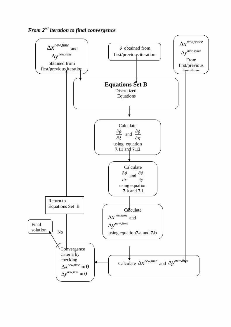
From 2nd

iteration to final convergence

Yes No

,new timex and ,new timey

obtained from

first/previous iteration

first iteration

obtained from

first/previous iteration

Equations Set B Discretized

Equations

Calculate

and

using equation

7.11 and 7.12

Calculate

x

and

y

using equation

7.k and 7.l

Calculate ,new timex and ,new timey

using equation7.a and 7.b

,new spacex

,new spacey

From

first/previous

iterations

Calculate ,new timex and

,new timey

Convergence

criteria by

checking , 0new timex

, 0new timey

Final

solution

Return to

Equations Set B

69

References

1. Introduction to computational fluid dynamics by A.W Date 105-171, 2005

2.“Fundamental of Heat and Mass Transfer” by Incorpera & Dewitt

3. Numerical Heat Transfer and Fluid Flow by Suhas .V. Patankar 71- 129,1980

4. Computational fluid dynamics: the basics with applications John D. Anderson,

Jr.(McGraw-Hill series in mechanical engineering--McGraw-Hill series in nautical and

aerospace engineering) 168-208, 1995

5. An introduction to computational fluid dynamics. The finite volume method. H.

K.VERSTEEG and W. MALALASEKERA

6. Software used MATLAB & Microsoft Word