Adaptive Grid Refinement Procedures for Efficient Optical Flow Computation

International Journal of Computer Vision 61(1), 31–54, 2005c© 2005 Springer Science + Business Media, Inc. Manufactured in The Netherlands.

Adaptive Grid Refinement Procedures for Efficient OpticalFlow Computation

JOAN CONDELLSchool of Computing and Intelligent Systems, Faculty of Engineering, University of Ulster, Magee College,

Northland Road, Londonderry, BT48 7JL, Northern [email protected]

BRYAN SCOTNEY AND PHILIP MORROWSchool of Computing and Information Engineering, Faculty of Engineering, University of Ulster at Coleraine,

Cromore Road, Coleraine, BT52 1SA, Northern [email protected]; [email protected]

Received January 2, 2002; Revised November 25, 2003; Accepted March 25, 2004

First online version published in September, 2004

Abstract. Two approaches are described that improve the efficiency of optical flow computation without incurringloss of accuracy. The first approach segments images into regions of moving objects. The method is based on apreviously defined Galerkin finite element method on a triangular mesh combined with a multiresolution segmenta-tion approach for object flow computation. Images are automatically segmented into subdomains of moving objectsby an algorithm that employs a hierarchy of mesh coarseness for the flow computation, and these subdomainsare reconstructed over a finer mesh on which to recompute flow more accurately. The second approach uses anadaptive mesh in which the resolution increases where motion is found to occur. Optical flow is computed over areasonably coarse mesh, and this is used to construct an optimal adaptive mesh in a way that is different from thegradient methods reported in the literature. The finite element mesh facilitates a reduction in computational effort byenabling processing to focus on particular objects of interest in a scene (i.e. those areas where motion is detected).The proposed methods were tested on real and synthetic image sequences, and promising results are reported.

Keywords: adaptive grids, Delaunay algorithm, inverse finite elements, motion estimation, optical flow, triangularmeshes

1. Introduction

The estimation of gray-level derivatives is of greatimportance to the analysis of image sequences forthe computation of velocity. Optical flow computationhas been proposed as a pre-processing step for manyhigh-level vision algorithms. Intensity-based differen-tial techniques have frequently been used to computevelocities from spatio-temporal derivatives of imageintensity or filtered versions of the image (Fennemaand Thompson, 1979; Horn and Schunck, 1981; Nagel,

1983). Horn and Schunck (1981) present an iterativealgorithm to find the optical flow pattern in which thederivatives of image intensity are approximated using afinite volume approach. They assumed the apparent ve-locity of the brightness pattern varied smoothly almosteverywhere in the image.

The approach used here begins with the problemwhere the apparent velocity of intensity patterns canbe directly identified with the movement of surfaces inthe scene. The finite volume approach used to developthe Horn and Schunck algorithm requires a regular

32 Condell, Scotney and Morrow

sampling of image intensity values stored in sim-ple rectangular arrays. In our algorithm a finite el-ement technique is used to approximate the imageintensity derivatives with a triangular discretisationimplementation (Axelsson and Barker, 2001). This fa-cilitates the development of algorithms which were pre-sented in previous work (Condell et al., 2001a) that aresufficiently general to be capable of tackling problemsin which the image is sampled non-uniformly, by theuse of non-uniform finite element meshes. Attentionis focused here on areas of motion within the imageby using various levels of grid coarseness to identifyregions with significant object movement to make thealgorithm more efficient yet still accurate.

A drawback of the gradient-based optical flowmethod of Horn and Schunck is that it does not preservemotion boundaries (Horn and Schunck, 1981). The al-gorithm is not satisfactory in cases where there arediscontinuities in the velocity field since the smooth-ness constraint leads to iterative equations that blur theabrupt changes in the velocity field. It is expected thatdiscontinuities occur in the optical flow where one ob-ject occludes another object and that problems can arisewith occluding edges in an algorithm based on this typeof smoothing constraint. Spatial and temporal alias-ing and problems with the existence of discontinuitiesare issues that are not addressed in this paper. The au-thors feel that these issues (such as blurring caused bysmoothing) need to be handled separately and so willbe addressed in future work.

The finite element algorithm is described inSection 2. Related research is considered in Sections 3and 4. An approach is proposed in Section 5 for multi-level grid segmentation and also an adaptive grid re-finement approach is proposed for the computation ofoptical flow. These methods use variants of the triangu-lar finite element algorithm (FETTRI) (Condell et al.,2001a). Experimental results with real and syntheticgray-scale images are shown in Section 6, and conclu-sions are discussed in Section 7.

2. Finite Element Solution

Computational efficiency can be greatly increased byfocusing only on those regions of the image sequencein which motion is detected to be occurring. This re-quires the ability to work with images in which theintensity values are sampled more frequently in areasof interest, such as localised regions of high intensitygradient or rapid variation of intensity with time, than

in areas likely to correspond to scene background. Forexample, Kirchner and Niemann (1992) used variationto facilitate the adaptive partitioning of the image forthe estimation of optical flow. The norm of the opticalflow in the direction of the image gradient has also beenused to generate an adaptive grid (Cohen and Herlin,1999).

Implementations based on finite difference or fi-nite volume methods become complicated to gen-eralise when the image intensity values are notuniformly sampled because they are based on point dif-ferences along regular co-ordinate directions. In con-trast, finite element methods are ideally suited for usewith variable and adaptive grids, and hence providethe basis of our framework for developing algorithmsto work with non-uniformly sampled images (Kirchnerand Niemann, 1992; Scotney, 1991). Benayoun and Ay-ache (1998) used the finite element method to solve theenergy minimisation problem for computing displace-ment vector fields where the resolution of their adaptivemesh depended on the value of the gradient intensity.

Non-uniformly sampled images may arise from theapplication of image compression techniques (Garciaet al., 1999; Yang et al., 2001). The inverse finite el-ement method that we develop has the advantage ofease of implementation via well-established finite ele-ment procedures, a rigorous mathematical formulation,along with conceptual simplicity.

2.1. Two Dimensional TriangularMesh Implementation

It has previously been shown (Graham et al., 2000a)that the algorithm of Horn and Schunck for opticalflow estimation may be considered as one of a familyof methods that may be derived using an inverse finiteelement approach. Two-dimensional Galerkin bilinearand triangular finite element techniques for optical flowestimation (FETBI, FETTRI) have been developed andextensively compared with the Horn and Schunck al-gorithm, as well as the best of the existing motion es-timation methods reported in the literature (Condellet al., 2001b; Graham et al., 2000b). They are shownto perform well.

This paper focuses on the development of techniquesbased on the triangular finite element mesh (Condellet al., 2001a). Triangular elements are known to give agood partition with a smaller ratio of nodes to elements,so may be considered superior to bilinear elements inthis regard (Devlaminck, 1995; Wang and Lee, 1996).

Adaptive Grid Refinement Procedures for Efficient Optical Flow Computation 33

Rectangular elements have been used in finite elementimage processing algorithms though it has been sug-gested that triangular elements could alleviate somenegative effects which were experienced in such algo-rithms (Yaacobson and Givoli, 1998).

2.2. Optical Flow Computation

In the inverse problem with which we are concerned,the image intensity values are known, and it is thevelocity function b, or optical flow, that is unknownand is to be approximated. The image intensity at thepoint (x, y) in the image plane at time t is denoted byu(x, y, t), which is considered to be a member of theHilbert space H 1 (image space) at any time t > 0. Theoptical flow is denoted by b ≡ (b1(x, y, t), b2(x, y, t))where b1 and b2 denote the x and y components ofthe flow b at time t > 0. The optical flow constraintequation is

ux b1 + uyb2 + ut = 0, (1)

where ux , uy, ut are the partial derivatives of the imageintensity with respect to x, y and t respectively.

Equation (1) cannot fully determine the flow but cangive the component of the flow in the direction of theintensity gradient. An additional constraint must be im-posed to ensure a smooth variation in the flow acrossthe image. The computation of optical flow may thenbe treated as a minimisation problem for the sum ofthe errors in the equation for the rate of change of im-age intensity and the measure of the departure fromsmoothness in the velocity field. This results in a pairof equations, which along with an approximation oflaplacians of the velocity components, allow the opti-cal flow to be computed.

2.3. Triangular Mesh Generation Scheme

Our first algorithm uses a finite element discretisationof the image domain � based on a regular array of right-angled isosceles triangles. Nodes are placed at the pixelcentres, and this array of nodes is used by a 2D Delau-nay algorithm to produce a triangular mesh, allowingthe partitioning of the image into elements for a regularpixel array, with nodes located at the three vertices ofthe triangular elements, as illustrated in Fig. 1. There-fore the triangles correspond to elements in the domaindiscretisation.

Figure 1. Regular triangular array of pixels and elements for finiteelement discretisation.

Figure 2. “Surrounding elements” for element ek in triangular dis-cretisation.

The element numbering provided by the Delaunayalgorithm is, as shown in Fig. 2, locally random. Whenconsidering the flow on a particular element ek (seeFig. 2), we must take account of the elements thatshare a node with ek (i.e. the “surrounding elements”).Only the contributions from these particular elementsare included in the equation for the flow over elementek (these “surrounding elements” for element ek are:e6, e3, e5, e1, e11, e7, e9, e10, e8, e12, e16 and e17).

2.4. Algorithm Formulation

The function space H 1 is infinite dimensional andtherefore cannot be used directly to provide a tractablecomputational technique. However, a function in theimage space H 1 may be approximately represented by afunction from a finite dimensional subspace Sh ⊂ H 1.From Sh a finite basis {φ j }N

j=1 is selected. Here, eachbasis function φi is associated with node i in that φi

has value 1 at node i and value zero at all other nodes,and is linear on each element. Hence the support ofφi is restricted to a neighbourhood �i consisting of


those elements that have node i as a vertex (the do-main in which φi is non-zero). The image u may thusbe approximately represented at time tn by a functionU n ∈ Sh , where U n = Z N

j=1U nj φ j and in which the

parameters {U nj }N

j=1 are mapped from the sampled im-age intensity values at time t = tn . A set of test func-tions, within Sh, may then be formed by associatingwith each element e, a test function �e(x, y) whichhas support limited to element e and those elementssurrounding e. For example, for element ek, �ek hassupport over the 13 elements shown in Fig. 2 (elementse6, e3, e5, e1, e11, e7, e9, ek, e10, e8, e12, e16 and e17).

The motion estimation equations for this FETTRI al-gorithm may thus be formed by associating with eachelement e, the test function �e(x, y) = φ1(x, y) +φ2(x, y) + φ3(x, y) such that �e(x, y) = 1 over ele-ment e, �e(x, y) = 0 over all elements other than thosesurrounding element e, and �e(x, y) falls linearly from1 to 0 over the elements that surround element e. Herethe nodes of element e are locally labelled 1, 2 and 3 asillustrated for element ek in Fig. 2. This test function�e(x, y) is thus a “plateau” function and has supportlimited to a neighbourhood consisting of only those tri-angular elements which share one of the three verticesof element e.

With the triangular mesh computed, it is possible tocompute the 2D velocity over the image by consider-ing the components of the optical flow to be piecewiseconstant over each element. An Euler forward finitedifference

U n+1j −U n

j

�t approximates the partial derivative∂U n

j

∂t , where U nj and U n+1

j are image intensity values inthe nth and (n + 1)th images respectively. The motionestimation equations

(1 − θ )N∑

j=1

U n+1j

∫�

[b1 · ∇φ j�e + b2 · ∇φ j�e]d�

+ θ

N∑j=1

U nj

∫�

[b1 · ∇φ j�e + b2 · ∇φ j�e]d�

+N∑

j=1

[U n+1

j − U nj

�t

] ∫�

φ j�ed� = 0, (2)

are based on a weak form of Eq. (1) and provide an ap-proximation to the optical flow constraint equation inwhich each equation contains unknown velocity com-ponent values. The parameter θ is chosen to help withthe stability of the numerical method and in our ex-periments we chose θ = 1

2 to correspond to Crank-Nicholson time stepping. Using the motion equationsof Eq. (2) in a Horn and Schunck style iteration, that

includes a smoothing term based on laplacians of thevelocity components, results in a pair of equations forthe optical flow for each triangular element in the mesh.A smoothing parameter α is incorporated into the mo-tion equations and an iteration procedure with a toler-ance value (toler) is used to ensure convergence to asolution.

3. Segmentation Using Motion Estimation

One of the most important preliminary steps leading tothe possibility of analysing images is to group pixelstogether into regions of similarity, i.e. segmentation.This involves segregating regions of similarity fromdissimilar regions so that distinct objects are simulta-neously characterised by various visual attributes, oneof which is motion. The problem is to find a subdivisionof the image that corresponds to the objects that appearin it (Yaacobson and Givoli, 1998). The main focus ofthis paper is to make FETTRI more efficient yet stillaccurate, and one way in which this can be done isby allowing the algorithm to use various levels of gridcoarseness. In the first algorithm proposed the image issegmented into regions of significant object movement,through these levels, on which subsequent processingis focussed. Hence we achieve a much lower computa-tional cost than running the algorithm uniformly overthe whole image.

Some research has been carried out on segment-ing images into moving regions using motion esti-mation (Choi and Kim, 1996). Illgner and Muller(1997) looked at segmenting images into homoge-neously moving regions using a criterion based on themotion estimate only, which was found through a hi-erarchical block matching approach. Goh and Martin(1994) presented a hierarchical region-growing algo-rithm which could segment the flow field into homoge-nous regions while Giachetti and Torre (1996) deriveda multiscale differential approach for estimating flowand extracting the motion edges. Schnorr (1991) usedthe finite element method over a uniform grid of tri-angular and quadrangular elements with linear and bi-linear shape functions to approximate weak solutionsin irregularly shaped domains. The motion boundarywas computed by decomposing the image plane intotwo disjoint sets (the uniform mesh and the segmentedobjects) separated by a smooth and closed curve.Yaacobson and Givoli (1998) considered the image seg-mentation problem using an h-adaptive finite elementmethod to solve the problem.


4. Multiresolution Approaches to Optical Flow

An effective approach to motion estimation is to em-bed gradient approaches in a hierarchical or multi-resolution scheme (Anandan, 1989). Hierarchical finiteelement and multiresolutional approaches have beenapplied previously to optical flow estimation problems(Cohen and Herlin, 1999; Moulin et al., 1997). It isknown that computational efficiency could be easedconsiderably by focusing on only those regions inwhich motion can occur without expending effort oncomputing flow for regions in which there is no mo-tion (Moulin et al., 1997; Schnorr, 1991). With finiteelement methods spatial discretisation is an importantissue as it defines the accuracy of the solution and nu-merical complexity of the algorithm. As mentionedpreviously, the main focus here is on improving theefficiency of the FETTRI algorithm. Computation canbe speeded up greatly by reducing the number of nodesin the system, so having a high density of nodes nearthe relevant regions of the image and a low density ofnodes for the background of the image. A multiresolu-tional approach would reduce significantly the numberof nodes and subsequent computational cost in this waywithout loss of accuracy, so increasing the overall effi-ciency of the FETTRI algorithm.

4.1. Multiresolutional Image Pyramid Approaches

Generally multiscale approaches are more computa-tionally efficient than single scale approaches andlead to consistent estimates at different spatial scales.Beauchemin and Barron (1995) considered hierarchi-cal processing that involved applying optical flowtechniques in a hierarchical, coarse-to-fine frame-work. Gaussian or Laplacian image pyramids havebeen used previously in block matching (Xie et al.,1996), correlation-based (Heeger, 1987), energy-based(Bergen et al., 1990) and differential frameworks(Anandan, 1989; Hwang and Lee, 1993; Terzopoulos,1986; Weber and Malik, 1995). Velocity estimateswere cascaded through each resolution level as ini-tial estimates subject to refinement. The final esti-mates were obtained when the refinement reached thefinest level of resolution. Enkelmann discussed multi-grid approaches in terms of choice of image pyra-mids and top-down strategies where coarse grid re-sults were used as starting vector fields for finer grids(Enkelmann, 1988). Control pyramid algorithms cansuffer from propagation of coarse motion estimation

errors to the finer levels of the pyramid (Moulin et al.,1997).

Multiresolutional methods have been used to mea-sure spatial and temporal brain deformation from se-quential Magnetic Resonance Images (MRI) usinga volumetric optical flow measurement (Hata et al.,1999). Moulin and Loui (1993) presented an itera-tive coarse-to-fine multiresolution method based on alinear combination of Yserentant’s hierarchical basis-function finite elements for estimating optical flow forvideo coding applications.

4.2. Adaptive Grid Refinement Approaches

Standard multiscale or multigrid approaches may notimprove optical flow estimates sufficiently. Differentscales can provide conflicting information. Most mul-tiresolution approaches have a uniform coarse-to-finesampling where new nodes are added regardless of theproblem being solved. Adaptive multiscale approachesmay be more suitable where discretisation scale is cho-sen locally according to the actual velocity estimatesthemselves or errors of velocity estimates.

Benayoun and Ayache (1998) introduced a match-ing contour method for computing flow by using finiteelement methods over an adaptively structured rectan-gular mesh in which the resolution depended on thepresence of high gradient norm points and/or high cur-vature points. Also Battiti et al. (1991) defined an adap-tive coarse-to-fine strategy for computing optical flowusing rectangular elements where the rectangular dis-cretisation grid was chosen depending on a reliabilitymeasure of the information derived at a given scale. Thealgorithm started by estimating the flow field at a rea-sonably coarse scale and improving this approximationon successively finer scales only in regions where theestimated error was greater than a predefined threshold.During tests it was revealed that the total error reacheda minimum on the middle of these scales of resolu-tion used in the resolution pyramid. Memin and Perez(1998) estimated motion using an adaptive multigridapproach, minimising an energy function through anappropriate hierarchy of subspaces of the whole con-figuration space. The adaptive rectangular structure re-lied on a subdivision criteria where a patch was splitin four if the standard deviation of the data outliers onthat patch exceeded a specified threshold.

Szeliski and Shum (1996) used a quadtree splinemultiresolution representation to compute flow. Patchsizes were automatically adapted to the complexity of


the underlying flow based on thresholded residual er-rors of the flow. They solved their system using gradientdescent and worked on a bilinear grid. At each levelof their image pyramid they carried out only 9 itera-tions at 3 different resolutions (sets of 4 × 4, 16 × 16and 64 × 64 pixels respectively). Other specific con-ceptual differences exist between the work of Szeliskiand Shum (1996) and the algorithms proposed in thispaper in the basics of the implementation and asso-ciated ideas involved. Szeliski and Shum developedtheir mesh based on the thresholding of a residual er-ror whereas in this work it is the actual velocity valuesthat are thresholded to create the adaptive mesh. AlsoSzeliski and Shum imposed continuity using interpola-tion of splines but the methods herein proposed developa piecewise constant velocity solution on each element.Consequently they essentially use a different image andvelocity representation in the form of a pointwise repre-sentation, using nodal point values of velocity obtainedfrom the underlying spline representation. In the meth-ods proposed in this paper a finite element approach istaken where the functional representation is in the weakform giving a functional (piecewise constant) form forthe velocities. Such finite element approaches are easilyextended to irregular grids which is much more diffi-cult with methods such as that of Szeliski and Shum(1996).

In terms of triangular elements, Kirchner andNiemann (1992) used the finite element method to com-pute optical flow with triangular regions. A fine parti-tion was used at motion boundaries ensuring a high res-olution flow field and a rough partition at areas whichwere homogeneous in time and space. They used anoriented smoothness constraint leading to a variationalproblem which they solved using successive overre-laxation. Elements were subdivided, if the graylevelgradient variance and the area were greater than thresh-olds. The tri-angulation process started with just twotriangles over the whole image. Similarly, Cohen andHerlin (1999) defined a framework for computing opti-cal flow using finite elements where an appropriate tri-angular tessellation of the image according to the normof the velocity in the direction of the image gradientimproved accuracy and yielded more reliable flows. Acoarse-to-fine multiresolution strategy was employedlocally increasing the resolution of the grid accordingto the particular image. The method was based on arecursive subdivision of a given tessellation of the do-main based on a splitting strategy. The flow they ob-tained did not seem correct over all areas especially in

regions where the norm measure could pass the pre-defined threshold falsely. Even where motion was notoccurring, some elements were still subdivided due tothe spatial or temporal gradient values. Consequently,Cohen and Herlin’s algorithm added in fine sections ofgrid coarseness in regions where motion did not oc-cur because the method detected high gradient or con-trast points which did not always correspond to motion.Conversely motion was missed where the image con-trast was insufficient to prompt element subdivision.

5. Proposed Approaches

Multiresolutional approaches are proposed where afamily of grids at increasing resolutions is used to makethe FETTRI algorithm more efficient. A basic segmen-tation algorithm is proposed in Section 5.1 based onthe computed optical flow over regular triangular grids.Further, an adaptive grid refinement algorithm for flowcomputation is proposed in Section 5.2 to make theFETTRI algorithm more efficient by increasing thedensity of nodes where motion occurs on non-uniformgrids. Some of the ideas from the literature reviewed inSections 3 and 4 will overlap with ideas used in meth-ods proposed in Sections 5.1 and 5.2. Methods avail-able in the literature will be compared and contrastedwith methods proposed where results are available andappropriate.

5.1. Hierarchical Segmentation Algorithm

A new implementation of the triangular technique(FETTRI) is now described which allows computa-tional activity to focus on segmented domains of mainmovement. It uses various levels of grid coarseness toidentify regions of interest corresponding to movementof independent objects, and generates new images ofthese regions from which flow is recomputed. This ba-sic concept is different to those used in state-of-the-art algorithms discussed in the segmentation literaturereviewed in Section 3. Regions are segmented usingprior knowledge on areas of main motion. A similarapproach was used by Wu and Kittler but which wasbased on different criteria (1993). Initially a coarse dis-cretisation is used here (see Fig. 3). To increase effi-ciency the fine discretisation is used subsequently onlyon particular regions of movement. Each added noderefines the grid in a region of interest and increasesthe numerical accuracy of the solution. As motion is


Figure 3. Hierarchy of finite elements at two scales—fine andcoarse discretisation.

recomputed on finer subimage grids so the recomputedflows are more accurate than the previous coarse gridapproximation over the full image. Figure 3 shows anexample of a coarse and fine discretisation achievedwith Delaunay random element orientation.

The following steps are involved in the region ex-traction algorithm:

1. Compute velocity fields for full image using coarsediscretisation.

2. Scan the velocity from the coarse grid to see if afiner triangulation is needed over independent re-gions of movement. The main region of movementis detected by focusing on extremities in magnitudeof optical flow from the coarse grid. An area is au-tomatically thresholded around this main region ofmovement by scanning the velocities in neighbour-ing elements.

3. After the main object of movement is segmentedthe remaining velocity from the image is scannedrecursively using Step 2 to segment further movingobjects. New thresholds are defined for further ob-jects which are based on a fraction of their velocitymagnitude extremities. Then proceed with Step 4.

4. Apply a standard boundary to the region of interestand adapt this area onto the fine grid. Compute ve-locity fields for segmented moving objects using afine discretisation.

5.2. Adaptive Grid Refinement Algorithmfor Flow Computation

Computation can be speeded up not only by reducingthe image size to subregions of movement of the orig-inal image, but also by reducing the number of nodesin the original image. For this purpose we develop amesh where the density of nodes is high in relevant

regions of the image and low in the background. Thiswill decrease the numerical complexity of the solutionby reducing both the number of elements and nodeswhile preserving accuracy. An adaptive grid refinementimplementation of the triangular technique (FETTRI)is now described which allows computational activ-ity to focus on regions of main movement. Generallythis adaptive mesh should allow a reduction in compu-tational requirements without decreasing accuracy offlow fields. A fine partition is used in areas of motion,ensuring a fine resolution of optical flow, and a roughpartition is used in areas of little or no motion, reducingthe computational effort. Image decomposition usingtwo or three resolutions of grid is sufficient, as was alsofound by Giachetti and Torre (1996). Multigrid imple-mentation is simplified by having a 2: 1 decrease ingrid resolution between adjacent levels and by havingthe grid nodes on coarse grids coincide with grid nodeson the fine grid.

5.2.1. Grid Refinement Scheme. Similar to Battitiet al. (1991) this adaptive coarse-to-fine strategy con-structs a grid where the discretisation grid is chosendepending on information derived at a given scale butin the proposed method triangular elements are usedwhereas Battiti et al. (1991) used rectangular elements.In the proposed method the flow field is estimated at areasonably coarse scale and is improved on over suc-cessive finer scales only in regions of the image wherethe motion is found to occur. Therefore, given an imagedomain, we construct a multiresolution grid such thatthe grid resolution increases only over structures whichare found to be moving.

To commence the process a mesh is constructedwhose resolution depends on the presence and mag-nitude of very coarsely previously computed velocitiesover the whole image. The aim is therefore to con-struct an optimal mesh which will then be used to re-compute the optical flow more efficiently than wouldbe achieved by using the fine grid over the whole im-age. The levels of resolution used were very coarse(4×4 pixels), coarse (2×2 pixels) and fine (1×1 pix-els) (see Fig. 4) with an “underlying mesh” (choice of16 × 16 pixels, 8 × 8 pixels or 4 × 4 pixels) addedfor consistency. The resulting mesh are abbreviated16 − 4 − 2 − 1, 8 − 4 − 2 − 1 or 4 − 4 − 2 − 1 depend-ing on which underlying mesh is used, for example the16 − 4 − 2 − 1 mesh indicates a 16 × 16 underlyingmesh with very coarse (4 × 4), coarse (2 × 2) and fine(1 × 1) areas of discretisation.


Figure 4. Levels of mesh refinement in discretisation.

Similar to Cohen and Herlin (1999) a very coarsetessellation commences the grid development proce-dure but here nodes are added where motion is foundto occur whereas Cohen and Herlin subdivided cellsof the triangulation depending on whether the norm ofthe velocity in the image gradient direction, computedfrom a combination of temporal and spatial derivatives,was greater than a given threshold.

The ideas used here in this proposed adaptive methodare conceptually different from the state-of-the-artmethods discussed in the multiresolutional method lit-erature reviewed in Section 4. Triangular methods areused over an adaptive strategy where good accuracy isexpected, both visually and quantitatively. The adap-tive mesh resolution strategy is designed in such a wayto ensure fine areas only over main moving structuresallowing a significant reduction in algorithm complex-ity. Areas are adaptively refined if velocity is knownto occur whereas in other methods a gradient mea-sure thresholded regions for fine meshing. This repre-sents a methodological improvement as previous meth-ods (Cohen and Herlin, 1999; Kirchner and Niemann,1992) have produced areas of incorrect movementwhere stationary objects can be seen in the originalimage.

In the proposed adaptive method, at first the meshis empty and nodes are added at increasing levels ofresolution (see Fig. 5) in areas where velocity is found

Figure 5. Addition and retainment of nodes for mesh.

to occur from the velocity previously computed overthe very coarse mesh. In this way the density of nodesis increased over areas which involve movement in theimage.

The following steps are involved in the optical flowestimation algorithm:

1. Compute smoothed or “averaged” image by com-puting the average of each group of 16 pixels in theimage.

2. Compute velocity fields for full ”averaged” imageusing very coarse discretisation.

3. Scan the velocity from the very coarse grid to seehow fine a triangulation is needed over regions ofmovement. The approach taken is to add a nodeor further nodes around a specified node depend-ing on whether the velocity previously obtained atthat node passes thresholds set for each level of gridresolution. At each stage of this part of the algo-rithm the current mesh is checked before specifiednodes are added to see if these nodes already ex-ist in the current mesh, as the Delaunay algorithmused for meshing assumes that duplicate points areeliminated.

(a) Commence the mesh construction with anempty mesh and define thresholds for each levelof grid coarseness.


(b) RETAIN VERY COARSE NODE: Scan the ve-locity for each node comparing it initially withthe very coarse threshold; if the velocity at thatvery coarse node passes the threshold then re-fine the grid by retaining this very coarse node,as in Fig. 5(a).

(c) ADD COARSE NODES: Scan the velocity foreach node comparing it with the coarse thresh-old; if the velocity at that coarse node passesthe threshold then refine the grid by adding thiscoarse node as well as 8 nodes around this node,as in Fig. 5(b).

(d) ADD FINE NODES: Scan the velocity for eachnode comparing it with the fine threshold; if thevelocity at that fine node passes the thresholdthen refine the grid by adding this fine nodeas well as 16 nodes around this node, as inFig. 5(c).

(e) ADD UNDERLYING MESH AND BOUND-ARY NODES: Ap ply a standard “underlying”mesh of 16 × 16 nodes, 8 × 8 nodes or 4 × 4nodes and add a standard “boundary” mesh onthe edges of the discretisation if required.

(f) Combine all nodes from previous steps to forma list of nodes for the final adaptive triangularmesh.

4. Compute velocity fields over this newly constructedadaptive mesh using stability (convergence toler-ance: toler) and smoothing (α) parameters.

6. Experimental Results and Discussion

Real image sequences are used for analysis and the dis-placed frame difference is examined as a quantitativemeasure of optical flow quality (Barron et al., 1994;Graham et al., 2000b; Ong and Spann, 1999). The sec-

Figure 6. Rotating Rubic image and Hamburg Taxi image.

ond method (the adaptive flow computation method)is most appropriate for real images where a significantpart of the image is static however an example of con-tinuous flow distribution is also used to illustrate thegenerality of the approach. Synthetic images are lesssuited to predicting the robustness of estimation un-der real world conditions. For the real synthetic imagesequence example shown both the displaced frame dif-ference error and the angular and absolute errors areused as performance measures (Graham et al., 2000b;Ong and Spann, 1999). In the experiments carried out,convergence of the algorithm to a specified tolerance(toler) is used to terminate the iteration procedure.

The velocity values are calculated per element andso it was necessary to perform an averaging process onthe element velocities to obtain velocities per nodal po-sition when computing the displaced frame difference.For this purpose the velocities of the neighbouring el-ements of any node were averaged to give a velocityfor that node ensuring velocities exist for each nodalposition. With the adaptive flow the displaced framedifference and the angular/absolute errors are calcu-lated over the adaptive nodes only for which velocityhas been computed using the adaptive grid refinementscheme. Velocity is written as displacement per unittime: pixels/frame (pix/ f r ).

6.1. Image Sequences

Rotating Rubic Cube. A frame from the Rotating Ru-bic sequence is shown in Fig. 6. The Rubic cube isrotating counter-clockwise on a turntable. The motionfield induced by this rotational motion involves veloci-ties of less than 2 pix/fr. The velocities on the turntablerange from 1.2 pixels/frame to 1.4 pix/fr while the ve-locities on the cube range from 0.2 pix/fr to 0.5 pix/fr.


Hamburg Taxi Scene. This sequence is a street sceneinvolving four moving objects. A car is moving in thelower left, driving left to right, 3 pixels/frame, while ataxi near the centre of the image is turning the cornerat 1 pixel/frame. There is a pedestrian in the upper leftmoving down to the left, 0.3 pixels/frame, while a vanin the lower right, partially occluded by trees, is movingright to left, 3 pixels/frame. A frame from the originalsequence is shown in Fig. 6.

The texture-mapped fly-through sequence of theYosemite Valley is a, complex test case involving dif-ferent parts moving in different directions with a widerange of velocities, aliasing and occluding edges be-tween the mountains and at the horizon. A frame fromthe original sequence is shown in Fig. 7 along with thecorresponding actual flow field. Most methods (Barronet al., 1994; Ong and Spann, 1999) produce poor re-sults on this sequence. The motion in the lower left ismainly divergent with the fractal-based clouds translat-ing left to right with a speed of 2 pixels/frame. Speedsin the lower left of the image range between 4 and5 pixels/frame.

The Rotating Rubic sequence and the Hamburg Taxisequence are both used in experiments for proposedmethods although the Rotating Rubic sequence maynot be as appropriate for the adaptive grid refinementalgorithm as it has only one main region of movementwhereas the Hamburg Taxi sequence has four indepen-dent moving objects. Also the Yosemite Valley imagesequence is an example of continuous flow distributionused to merely illustrate the generality of the adaptiveapproach. It contains complex continuous flow withknown ground truth.

In experiments carried out the smoothing parameterα was used at varying levels. Different authors havesuggested different amounts of smoothness, often pre-defining the smoothing parameter randomly without

Figure 7. Yosemite Valley image and correct flow.

any further experimentation (Barron et al., 1994). Itwas found that the parameter needed to be chosen care-fully to enhance performance. Also results are shownfor the convergence tolerance value (toler) at differentlevels—0.001, 0.0001 and 0.00001. As before, oftenauthors in the literature have only carried out a cer-tain number of iterations, in which case there is a highlikelihood that the system has not converged to a truesolution (Aisbett, 1989; Barron et al., 1994; Bartoliniand Piva, 1997). Previous results on the basic FET-TRI algorithm have shown that iterating until conver-gence gives a much clearer understanding of the flow(Graham et al., 2000a, b).

6.2. Basic Results of FETTRI Algorithm

The results for the FETTRI algorithm, for convergencetolerance 0.001 and smoothing parameter α = 200, runon the original fine discretisation over the full imagefor the Rotating Rubic sequence and for a convergencetolerance 0.001 and α = 275 for the Hamburg Taxisequence are shown in Fig. 8.

Figure 9 shows the results for the FETTRI algorithmson the original fine discretisation over the full image forthe Yosemite Valley sequence. The results are shown forconvergence tolerance toler = 0.001 and toler = 0.0001respectively both with smoothing parameter α = 400.

Table 1 shows the displaced frame difference er-rors for the FETBI and FETTRI algorithms, using afine mesh over the whole image, compared with otheralgorithms reported in the literature (Anandan, 1989;Horn and Schunck, 1981; Nagel, 1983; Ong and Spann,1999). The use of the mean absolute displaced framedifference error is known to give an overall quantita-tive comparison but should not be taken as a detailedquantitative indication of how well the estimated flow


Figure 8. Rotating Rubic (0.001; 200) and Hamburg Taxi (0.001; 275) fine grid averaged flow.

Figure 9. Yosemite Valley fine grid FETTRI flows (0.001; 400) and (0.0001; 400).

correlates with the true flow. Using the displaced framedifference error as a quantitative comparison, it can beseen from Table 1 that the FETTRI algorithms’ perfor-mance compares well with that of other techniques onthese sequences and shows a clear improvement overthe FETBI algorithm.

Table 2 shows the mean angular and absolute errormeasures for the synthetic Yosemite Valley sequence

Table 1. Displaced frame difference (DFD) error values for Hamburg Taxi, RotatingRubic and Yosemite Valley image sequences with FETBI, FETTRI and other algorithms.

Mean forward DFD (toler; α)

Algorithm Rotating rubic Hamburg taxi Yosemite valley

FETBI fine (0.001; 400) (0.001; 75) (0.001; 75)(Whole image) 2.71 3.53 11.08

FETTRI fine (0.001; 200) (0.001; 275) (0.001; 400)(Whole image) 1.58 3.19 10.94

Anandan (1989) 5.31 4.35

Fleet and Jepson (1989) 4.42 6.20

Horn and Schunck (1981) 1.98 4.01

Lucas and Kanade (1981) 2.11 3.99

Nagel (1983) 3.28 4.21

Odobez and Bouthemy (1994) 2.06 3.93

Ong and Spann (1999) 1.97 3.84

on the FETBI (Graham et al., 2000a) and other algo-rithms. The results show satisfactory and comparableerror values for this complex and difficult test case.

Further experimentation (Graham et al., 2000a, b)has shown that the Rotating Rubic sequence requiresa medium value of α(α = 200) for satisfactory per-formance while the Hamburg Taxi sequence improveswith slightly higher α values. Conversely, high values


Table 2. Mean absolute and mean angular error values for YosemiteValley image sequence with FETBI and other algorithms.

Algorithm Mean absolute Mean angular(toler; α) error error Density

FETBI (0.0001;400) 1.40 33.40 100.00

Barron et al. (1994) 31.69 100.00

Black and 31.03 100.00Anandan (1996)

of α(α ≥ 400) result in only the taxi flow remaining forthe Hamburg Taxi sequence. The Yosemite Valley re-sults gave more visually accurate flow and lower errorsfor medium smoothing parameter α values (α = 400)with the FETTRI algorithm. The convergence tolerancelevel chosen for these experiments (0.001) was shownin previous experimentation (Graham et al., 2000a, b)to result in less propagation of flow to other areas.

6.3. Results of Hierarchical RegionExtraction Approach

The Hamburg Taxi sequence is used to illustrate the re-gion extraction algorithm described in Section 5.1, as

Figure 10. (a) Hamburg Taxi (coarse grid) flow (0.001; 275); (b) Hamburg Taxi taxi region (fine grid) flow (0.001; 150); (c) Hamburg Taxicar region (fine grid) flow (0.001; 75); (d) Hamburg Taxi van region (fine grid) flow (0.001; 400).

it involves four independently moving objects with dif-ferent velocities (car, van, taxi and pedestrian). Usingthe region extraction approach described in Section 5.1,we calculate the motion over a sequence using a coarsegrid. The flow results from this coarse grid are shown inFig. 10(a) for convergence tolerance 0.001 and smooth-ing parameter α = 275, from which we see that thethree main detected areas of movement correspond tothe van, the taxi and the car. A finer triangulation is thenneeded over these three regions, and so the region ex-traction algorithm was used to automatically generatethese areas of movement, as in Step 2 of the algorithmdetailed in Section 5.1.

The van is the first region to be extracted followed bythe taxi, then the car. These regions are reconstructedand their motion estimated on the fine. grid. Celasunet al. (2001) used the Hamburg Taxi sequence to evalu-ate their video object segmentation algorithm and sim-ilarly detected all three main moving objects, althoughthey did not further recalculate the motion for thesesegmented objects.

Estimates arising from the three main regions ofmovement are shown in Figs. 10(b)–(d) for the taxi, carand van regions respectively for respective α smooth-ing and convergence tolerance (toler) parameter values.Satisfactory results are shown for all three main moving


Table 3. Time (seconds) and iterations to convergence forHamburg Taxi image sequence with FETTRI basic and regionextraction algorithms.

Time and iterations

Discretisation Time (sec) Iter.

Fine grid: Full image (0.001; 275) 231 421

Coarse grid: Full image (0.001; 275) 51 364

Fine grid: Van region (0.001; 400) 14 249

Fine grid: Taxi region (0.001; 150) 21 266

Fine grid: Car region (0.001; 75) 11 799

Total:

Fine grid full image 231

Coarse grid full image

Plus 3 fine grid regions 97

objects according to what the correct flow should be.Further experimentation shows that too high smoothingα(α ≥ 600) and low toler values (0.0001) result in flowpropagation to regions of non movement.

The proposed region extraction algorithm gives theadded advantage of being able to use different α andtoler parameter values for the independent moving ob-jects in the sequence. In comparison to this, for theFETTRI algorithm run on the full images using afine grid it is necessary to used the same convergence

Table 4. Number of nodes and elements for specified threshold values for Hamburg Taxi imagesequence with FETBI, FETTRI basic and adaptive grid refinement algorithms.

Thresholds

Algorithm Very coarse Coarse Fine Nodes Elements

FETTRI Adaptive

16 − 4 − 2 − 1 0.1 0.8 1.5 973 1879

16 − 4 − 2 − 1 0.25 0.875 1.5 643 1247

8 − 4 − 2 − 1 0.05 0.15 0.25 7414 14544

8 − 4 − 2 − 1 0.1 0.55 1.0 1622 3145

8 − 4 − 2 − 1 0.25 0.875 1.5 695 1315

4 − 4 − 2 − 1 0.1 0.425 0.75 2738 5322

4 − 4 − 2 − 1 0.25 0.5 0.75 2558 4980

4 − 4 − 2 − 1 0.25 0.875 1.5 965 1827

FETBI∗ 12160 11938

FETTRI fine∗ 12160 23876

FETTRI coarse∗ 3072 5922

FETTRI very coarse∗ 768 1426

∗Regular non-adaptive mesh over whole image.

and smoothing values for the entire image, and conse-quently for all independent moving objects. Such an ap-proach for segmentation results in computing more sat-isfactory flow for some objects than for others. There-fore the region extraction and segmentation algorithmgives more versatility in being able to achieve satisfac-tory flows for all independent moving objects.

Table 3 shows the time savings for the region ex-traction algorithm for this Hamburg Taxi sequence. Itshows that running the algorithm with the coarse gridon the whole image followed by focusing on regionsof interest on the fine grid is much faster than runningthe algorithm on the fine grid over the whole image (97seconds compared with 231 seconds). Therefore an-other obvious advantage of this new region extractionapproach to the FETTRI algorithm is the efficiency im-provement in comparison with the original calculationson the fine grid, without loss of accuracy. Improvementin computational time is due to the smaller number ofequations to be solved on the coarse mesh than withthe fine mesh, as fewer elements exist on the coarsemesh (see Table 4: 5922 elements on the FETTRI uni-form coarse grid compared with 23876 elements onthe FETTRI uniform fine grid).

The number of iterations are also shown in Table 3.An important point to note here is that the algorithmis allowed to converge to a solution using a varyingnumber of iterations. Other authors specified a number


of iterations before testing (Szeliski and Shum, 1996).The results of Szeliski and Shum (1996) on the Ham-burg Taxi sequence showed a more dominant car flow,followed by the taxi, with only a slight van flow de-tected.

6.4. Results of Adaptive Grid Refinement Algorithm

The Hamburg Taxi, Rotating Rubic and Yosemite Val-ley sequences are used to illustrate the adaptive opti-cal flow estimation algorithm described in Section 5.2.An adaptive mesh was established using the algorithmdescribed in Section 5.2. The α, toler and thresholdparameters are chosen based on previous results fromthese sequences. The effects of changing these param-eters will be discussed.

An optical flow result from the Hamburg Taxi se-quence for convergence tolerance toler = 0.001 andsmoothing parameter α = 600 was used to commencethe construction process for the adaptive mesh usingvarious threshold parameters. A resulting 4−4−2−1adaptive mesh from this adaptive process with the4 × 4 underlying mesh for the Hamburg Taxi se-quence is shown in Fig. 11(a) for very coarse threshold0.1, coarse threshold 0.425 and fine threshold 0.75.We can observe that the mesh resolution is fine overthe three main moving structures, that is the taxi,van and car, allowing significant algorithmic com-plexity reduction. As the number of background el-ements is sparse so efficiency savings are achieved.Another mesh is shown for comparison for this se-quence with an underlying mesh of 8 × 8 pixels(8−4−2−1 adaptive mesh) for very coarse threshold

Figure 11. (a) Hamburg Taxi 4 − 4 − 2 − 1 mesh for very coarse threshold 0.1, coarse threshold 0.425, fine threshold 0.75; (b) Hamburg Taxi8 − 4 − 2 − 1 mesh for very coarse threshold 0.25, coarse threshold 0.875, fine threshold 1.5.

0.25, coarse threshold 0.875 and fine threshold 1.5 inFig. 11(b).

The corresponding flows for these two meshes areshown in Fig. 12 for convergence tolerance toler =0.0001, smoothing parameterα = 500 and convergencetolerance toler = 0.001, smoothing parameter α = 900respectively. It can be seen from these two meshes andflow results that the choice of thresholds greatly influ-ences the completed adaptive mesh. A higher coarseand fine threshold will result in coarser mesh resolu-tions for the main moving objects. Comparing theseresults to those of Cohen and Herlin (1999) this adap-tive grid refinement method successfully finds flow forall three main moving objects while Cohen and Her-lin’s method was not able to find the car flow due to lowcontrast. Similar to the proposed adaptive grid refine-ment method, Cohen and Herlin (1999) did not locatethe pedestrian’s flow.

Table 4 shows the efficiency savings in terms of num-ber of nodes and number of elements for these adaptivemeshes using the proposed grid refinement algorithmfor the Hamburg Taxi sequence. Various other combi-nations of 16−4−2−1, 8−4−2−1 and 4−4−2−1adaptive mesh are included comparing the number ofelements and nodes obtained for each mesh. The twomeshes and corresponding flows shown in Figs. 11 and12 are represented and highlighted in Table 4 fromwhich it can be seen that the 8 − 4 − 2 − 1 mesh forvery coarse, threshold 0.25, coarse threshold 0.875 andfine threshold 1.5 has the lowest number of elementsand nodes of these two meshes (695 nodes and 1315elements). This is a measure of the reduction in com-putational effort as the number of elements indicatesthe number of equations involved in the solution.


Figure 12. (a) Hamburg Taxi 4 − 4 − 2 − 1 flow for very coarse threshold 0.1, coarse threshold 0.425, fine threshold 0.75 (0.0001; 500); (b)Hamburg Taxi 8 − 4 − 2 − 1 flow for very coarse threshold 0.25, coarse threshold 0.875, fine threshold 1.5 (0.001; 900).

When compared to the number of elements andnodes necessary for the uniform mesh on the whole im-age for other FETBI and FETTRI algorithms these twoadaptive meshes of Fig. 11 both show that the adaptivegrid refinement approach proposed gives a significantreduction in computational effort (695 and 2738 nodesfor adaptive meshes of Fig. 11 respectively comparedwith 12160 nodes for the uniform FETBI and FETTRIfine mesh).

From Fig. 11 it is obvious that there is a signif-icant difference in the resulting mesh when using a4 − 4 − 2 − 1 structure and a 8 − 4 − 2 − 1 structure.Figure 11(a) shows the 4 − 4 − 2 − 1 mesh where thebackground or underlying mesh (4 × 4) is finer thanthat of Fig. 11(b) where an 8 × 8 underlying mesh isused. The 4 − 4 − 2 − 1 mesh allows much finer ar-eas of discretisation for the three main moving objects

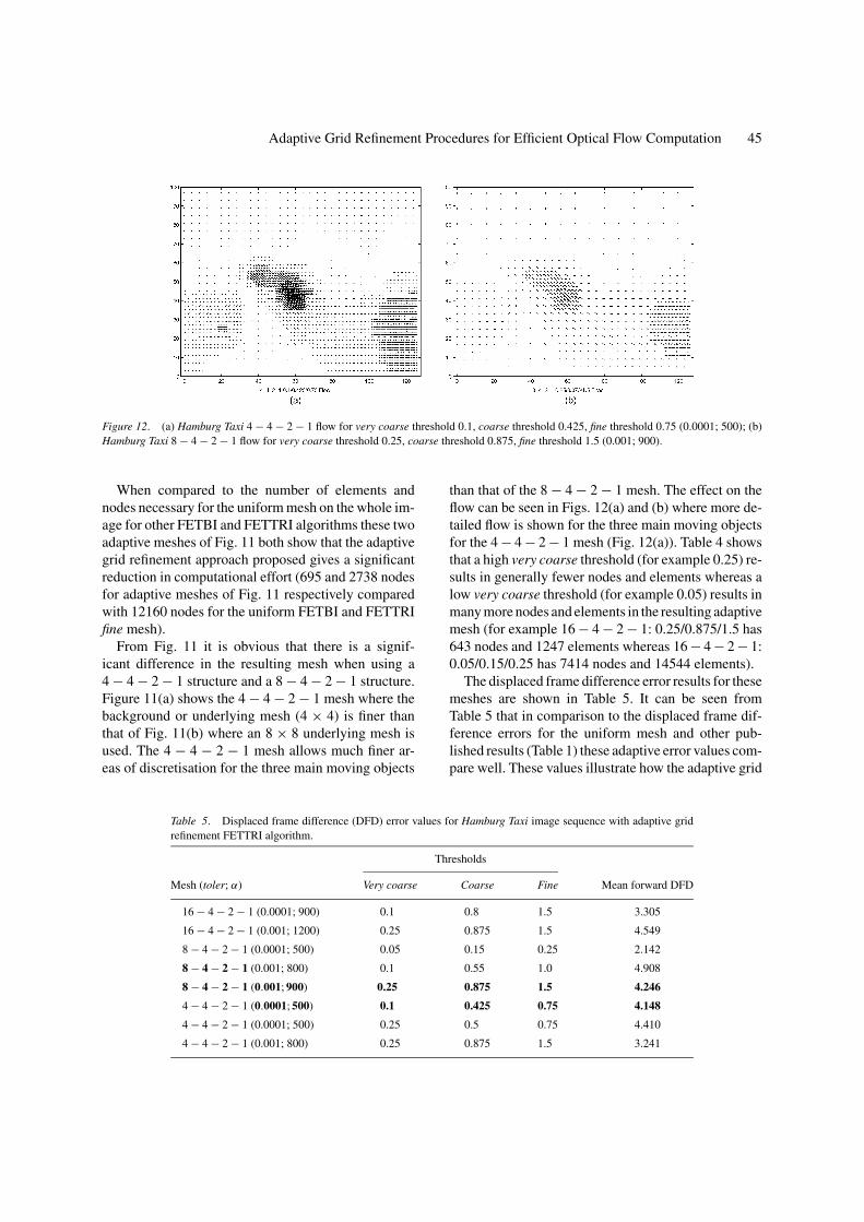
Table 5. Displaced frame difference (DFD) error values for Hamburg Taxi image sequence with adaptive gridrefinement FETTRI algorithm.

Thresholds

Mesh (toler; α) Very coarse Coarse Fine Mean forward DFD

16 − 4 − 2 − 1 (0.0001; 900) 0.1 0.8 1.5 3.305

16 − 4 − 2 − 1 (0.001; 1200) 0.25 0.875 1.5 4.549

8 − 4 − 2 − 1 (0.0001; 500) 0.05 0.15 0.25 2.142

8 − 4 − 2 − 1 (0.001; 800) 0.1 0.55 1.0 4.908

8 − 4 − 2 − 1 (0.001; 900) 0.25 0.875 1.5 4.246

4 − 4 − 2 − 1 (0.0001; 500) 0.1 0.425 0.75 4.148

4 − 4 − 2 − 1 (0.0001; 500) 0.25 0.5 0.75 4.410

4 − 4 − 2 − 1 (0.001; 800) 0.25 0.875 1.5 3.241

than that of the 8 − 4 − 2 − 1 mesh. The effect on theflow can be seen in Figs. 12(a) and (b) where more de-tailed flow is shown for the three main moving objectsfor the 4 − 4 − 2 − 1 mesh (Fig. 12(a)). Table 4 showsthat a high very coarse threshold (for example 0.25) re-sults in generally fewer nodes and elements whereas alow very coarse threshold (for example 0.05) results inmany more nodes and elements in the resulting adaptivemesh (for example 16 − 4 − 2 − 1: 0.25/0.875/1.5 has643 nodes and 1247 elements whereas 16 − 4 − 2 − 1:0.05/0.15/0.25 has 7414 nodes and 14544 elements).

The displaced frame difference error results for thesemeshes are shown in Table 5. It can be seen fromTable 5 that in comparison to the displaced frame dif-ference errors for the uniform mesh and other pub-lished results (Table 1) these adaptive error values com-pare well. These values illustrate how the adaptive grid


Figure 13. Hamburg Taxi forward displaced frame difference error vs. α smoothing parameter for adaptive grid refinement FETTRI algorithm4 − 4 − 2 − 1: 0.25/0.875/1.5 with convergence tolerance toler = 0.001 and toler = 0.0001.

refinement approach maintains accuracy while givingthis reduction in computational effort. The 4−4−2−1flow for very coarse, threshold 0.25, coarse threshold0.875 and fine threshold 1.5 results in forward displacedframe difference error 3.241, outperforming the otherliterature methods’ results of Table 1. Fig. 13 shows thisforward displaced frame difference error for the 4−4−2−1 adaptive flow (very coarse threshold 0.25, coarsethreshold 0.875 and fine threshold 1.5) plotted againstthe α smoothing parameter for both toler = 0.001 andtoler = 0.0001 convergence tolerance values.

Figure 13 shows the effect of the α smoothing param-eter on the results. It can be seen that for 500 ≤ α ≤ 900both toler = 0.001 and toler = 0.0001 give higherdisplaced frame difference errors which then drop toa near-constant level of error for α ≥ 900. FromTable 4 and Table 5, generally the mesh with the high-est number of nodes and elements results in the low-est displaced frame difference error (8 − 4 − 2 − 1 :0.05/0.15/0.25 has 7414 nodes and 14544 elementswith a displaced frame difference of 2.142) while themesh with the lowest number of nodes and elementsresults in one of the highest displaced frame differenceerrors (16 − 4 − 2 − 1 : 0.25/0.875/1.5 has 643 nodesand 1247 elements with a displaced frame differenceof 4.549). This suggests a trade-off in complexity andaccuracy.

Table 6 shows the convergence times and itera-tions for the adaptive meshes over the Hamburg Taxisequence compared to the uniform meshes over theFETBI and FETTRI algorithms. It can be seen thatthe adaptive algorithm generally takes much fewer it-erations to converge than the FETTRI algorithm andalso in a shorter time. The total number of iterationsperformed with this adaptive algorithm was mostly

Table 6. Time (seconds) and iterations to convergence for Ham-burg Taxi image sequence with FETBI, FETTRI and (specific thresh-old values) adaptive grid refinement FETTRI algorithms (toler/α).

Algorithm: Discretisation (toler/α) Time (sec) Iter.

FETBI

Uniform (0.0001/400) 31 1083

FETTRI

Uniform fine grid (0.0001/175) 1156 1891




∗(0.25/0.875/1.5; 4 − 4 − 2 − 1; 0.001/800) 4 130∗(0.25/0.875/1.5; 8 − 4 − 2 − 1; 0.001/900) 22 714∗(0.25/0.875/1.5; 16 − 4 − 2 − 1; 0.001/1200) 2 101

∗FETTRI adaptive non-uniform mesh over whole image.


between 100 and 130 iterations compared to the single-level fine resolution FETTRI algorithm which for ex-ample required often more than 1000 iterations to geta satisfactory solution of similar accuracy. Compar-ing node reduction against time reduction the adaptive8 − 4 − 2 − 1 mesh for very coarse threshold 0.25,coarse threshold 0.875 and fine threshold 1.5 has 695nodes and takes 22 seconds whereas the FETTRI uni-form fine grid has 12160 nodes and on average takesat least 1100 seconds to converge. This illustrates theimportant numerical complexity reduction and compu-tational efficiency improvement achieved through thisproposed adaptive grid refinement algorithm in com-parison with the FETTRI uniform algorithm.

An optical flow result from the Rotating Rubic se-quence for convergence tolerance 0.001 and smoothingparameter α = 600 was used to commence the con-

Figure 14. (a) Rotating Rubic 4 − 4 − 2 − 1 mesh for very coarse threshold 0.25, coarse threshold 0.525, fine threshold 0.8; (b) RotatingRubic 8 − 4 − 2 − 1 mesh for very coarse threshold 0.1, coarse threshold 0.55, fine threshold 1.0.

Figure 15. (a) Rotating Rubic 4 − 4 − 2 − 1 flow for very coarse threshold 0.25, coarse threshold 0.525, fine threshold 0.8 (0.0001; 700); (b)Rotating Rubic 8 − 4 − 2 − 1 flow for very coarse threshold 0.1, coarse threshold 0.55, fine threshold 1.0 (0.0001; 900).

struction process for the optimal mesh using variousthreshold parameters. A resulting 4−4−2−1 adaptivemesh from this adaptive process with the 4 × 4 under-lying mesh for the Rotating Rubic sequence is shownin Fig. 14(a) for very coarse threshold 0.25, coarsethreshold 0.525 and fine threshold 0.8. We can observethat the mesh resolution is fine over the main movingstructure, that is the turntable. Another mesh is shownfor comparison for this sequence with an underlyingmesh of 8 × 8 pixels (8 − 4 − 2 − 1 adaptive mesh) forvery coarse threshold 0.1, coarse threshold 0.55 andfine threshold 1.0 in Fig. 14(b). We can observe thatthe mesh resolution is fine over the main moving re-gions in the image, that is the turntable and the rotatingcube.

The corresponding flows for these two meshes areshown in Fig. 15 for convergence tolerance toler


= 0.0001, smoothing parameter α = 700 and conver-gence tolerance toler = 0.0001, smoothing parameterα = 900 respectively. It can be seen from these twomeshes and flow results that the different choice ofthresholds give the finest resolution in the same areaof the turntable where the largest velocity is retrieved.Comparing these results visually to those of Cohen andHerlin (1999) this adaptive grid refinement method isable to achieve a more consistent flow with what isknown to be the correct flow over this sequence. Aswith Cohen and Herlin’s method, Fig. 15 shows the flowfinely computed for the left hand side of the turntablewhile less finely computed flow for the turntables’ righthand side.

Table 7 shows the efficiency savings in terms of num-ber of nodes and number of elements for the adap-tive algorithm for this sequence. Table 7 again illus-trates the significant reduction in computational effort.Similar to the Hamburg Taxi sequence, when we com-pared the number of elements and nodes necessary forthe uniform mesh on the whole Rotating Rubic imagefor other FETBI and FETTRI algorithms, these twoadaptive Rotating Rubic meshes of Fig. 14 both showthat the adaptive grid refinement approach proposedadaptive gives a significant reduction in computationaleffort (1072 and 606 nodes respectively for Fig. 14compared to 15360 nodes for FETBI and FETTRIalgorithms).

Table 7. Number of nodes and elements for specified threshold values for Rotating Rubic image sequencewith FETBI, FETTRI basic and adaptive grid refinement algorithms.

Thresholds


FETTRI Adaptive

16 − 4 − 2 − 1 0.0375 0.144 0.25 4407 8747

16 − 4 − 2 − 1 0.1 0.8 1.5 430 819

8 − 4 − 2 − 1 0.025 0.263 0.5 1921 3730

8 − 4 − 2 − 1 0.1 0.55 1.0 606 1138

8 − 4 − 2 − 1 0.1 0.8 1.5 525 976

4 − 4 − 2 − 1 0.2 0.55 0.9 1041 1960

4 − 4 − 2 − 1 0.23 0.52 0.55 1288 2454

4 − 4 − 2 − 1 0.25 0.525 0.8 1072 2022

FETBI∗ 15360 15113


FETTRI coarse∗ 3840 7434

FETTRI very coarse∗ 960 1798


The accuracy maintained is illustrated in the dis-placed frame difference error results for these RotatingRubic meshes shown in Table 8. These values showthat in comparison to the displaced frame differenceerrors for the uniform mesh and other published results(Table 1) these adaptive error values compare well,illustrating the reduction in computational effort ob-tained with the adaptive grid refinement approachwhilst still maintaining accuracy.

Table 9 shows the convergence times and iterationsfor adaptive meshes over the Rotating Rubic sequencecompared to the uniform meshes over the FETBI andFETTRI algorithms. It can be seen that the adaptive al-gorithm generally takes much fewer iterations to con-verge than the FETTRI algorithm and also in a shortertime. The total number of iterations performed withthis adaptive algorithm was mostly between 90 and400 iterations compared to the single-level fine reso-lution FETTRI algorithm which for example requiredoften more than 1500 iterations to get a satisfactorysolution of similar accuracy. Comparing node reduc-tion against time reduction the adaptive 4 − 4 − 2 − 1mesh for very coarse threshold 0.2, coarse threshold0.55 and fine threshold 0.9 has 1041 nodes and takes22 seconds whereas the FETTRI uniform fine grid has15360 nodes and on average takes at least 728 sec-onds to converge. This again illustrates the importantnumerical complexity reduction and computational


Table 8. Displaced frame difference (DFD) error values for Rotating Rubic image sequence with adaptivegrid refinement FETTRI algorithm.

Thresholds


16 − 4 − 2 − 1 (0.001; 1200) 0.0375 0.144 0.25 1.739

16 − 4 − 2 − 1 (0.001; 1600) 0.1 0.8 1.5 1.434

8 − 4 − 2 − 1 (0.0001; 900) 0.025 0.263 0.5 2.365

8 − 4 − 2 − 1(0.0001; 900) 0.1 0.55 1.0 1.928

8 − 4 − 2 − 1 (0.0001; 1000) 0.1 0.8 1.5 1.238

4 − 4 − 2 − 1 (0.0001; 600) 0.2 0.55 0.9 1.227

4 − 4 − 2 − 1 (0.0001; 600) 0.23 0.52 0.55 2.156

4 − 4 − 2 − 1(0.0001; 700) 0.25 0.525 0.8 1.261

Table 9. Time (seconds) and iterations to convergence for Ro-tating Rubic image sequence with FETBI, FETTRI and (specificthreshold values) adaptive grid refinement FETTRI algorithms(toler/α).

Algorithm: Discretisation (toler/α) Time (sec) Iterations

FETBIUniform (0.0001/200) 23 779

FETTRIUniform fine grid (0.0001/200) 929 1572



Uniform fine grid (0.0001/800) 1254 1983∗(0.2/0.55/0.9; 4 − 4 − 2 − 1; 0.0001/600) 22 349∗(0.2/0.55/0.9; 8 − 4 − 2 − 1; 0.001/1200) 2 99∗(0.2/0.55/0.9; 16 − 4 − 2 − 1; 0.0001/1800) 22 391

∗FETTRI adaptive non-uniform mesh over whole image.

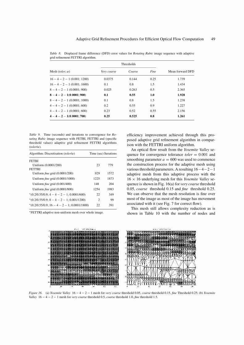
Figure 16. (a) Yosemite Valley 16 − 4 − 2 − 1 mesh for very coarse threshold 0.05, coarse threshold 0.15, fine Threshold 0.25; (b) YosemiteValley 16 − 4 − 2 − 1 mesh for very coarse threshold 0.5, coarse threshold 1.0, fine threshold 1.5.

efficiency improvement achieved through this pro-posed adaptive grid refinement algorithm in compar-ison with the FETTRI uniform algorithm.

An optical flow result from the Yosemite Valley se-quence for convergence tolerance toler = 0.001 andsmoothing parameter a = 600 was used to commencethe construction process for the adaptive mesh usingvarious threshold parameters. A resulting 16−4−2−1adaptive mesh from this adaptive process with the16 × 16 underlying mesh for this Yosemite Valley se-quence is shown in Fig. 16(a) for very coarse threshold0.05, coarse threshold 0.15 and fine threshold 0.25.We can observe that the mesh resolution is fine overmost of the image as most of the image has movementassociated with it (see Fig. 7 for correct flow).

This mesh still allows complexity reduction as isshown in Table 10 with the number of nodes and


Table 10. Number of nodes and elements for specified threshold values for Yosemite Valley imagesequence with FETBI, FETTRI basic and adaptive grid refinement algorithms.

Thresholds


FETTRI adaptive

16 − 4 − 2 − 1 0.025 0.263 0.5 11581 22917

16 − 4 − 2 − 1 0.0375 0.144 0.25 13907 27554

16 − 4 − 2 − 1 0.05 0.15 0.25 13906 27552

16 − 4 − 2 − 1 0.1 0.8 1.5 4608 9037

16 − 4 − 2 − 1 0.2 0.55 0.9 8188 16146

16 − 4 − 2 − 1 0.25 0.875 1.5 4374 8570

16 − 4 − 2 − 1 0.5 1.0 1.5 4006 7842

FETBI∗ 19908 19625



elements for the various adaptive and non-adaptivemeshes (19908 nodes and 39250 elements for the FET-TRI fine mesh compared to 13906 nodes and 27552elements for this adaptive mesh). Another more sparsemesh is shown in Fig. 16(b) for comparison for thissequence for very coarse threshold 0.5, coarse thresh-old 1.0 and fine threshold 1.5. This mesh shows finerregions of elements for the upper region of the imageand shows more significant algorithmic complexity re-duction (4006 nodes and 7842 elements).

The corresponding flows for these two meshes areshown in Figs. 17(a) and (b) for convergence tolerancetoler = 0.0001 with smoothing parameters α = 600and convergence tolerance toler = 0.001 with smooth-ing parameters α = 1400 respectively. As for the pre-

Figure 17. (a) Yosemite Valley 16 − 4 − 2 − 1 flow for very coarse threshold 0.05, coarse threshold 0.15, fine threshold 0.25 (0.0001/600);(b) Yosemite Valley 16 − 4 − 2 − 1 flow for very coarse threshold 0.5, coarse threshold 1.0, fine threshold 1.5 (0.001/1400).

vious image sequences, it can be seen for these twomeshes and flow results for the Yosemite Valley se-quence that the choice of thresholds greatly influencesthe completed adaptive mesh.

The displaced frame difference error results for theseand other meshes on the Yosemite Valley sequence areshown in Table 11. It can be seen from Table 11 that incomparison to the displaced frame difference errors forthe uniform FETBI and FETTRI mesh (Table 1) theseadaptive error values show a significant improvement.These values illustrate how the adaptive grid refine-ment approach maintains (and here improves) accuracywhile giving this reduction in computational effort. Alldisplaced frame differences in Table 11 outperform thecorresponding errors in Table 1.


Table 11. Displaced frame difference (DFD) error values for Yosemite Valley image sequence with adaptivegrid refinement FETTRI algorithm.

Thresholds


16 − 4 − 2 − 1 (0.001; 800) 0.025 0.263 0.5 5.31

16 − 4 − 2 − 1 (0.0001; 600) 0.0375 0.144 0.25 5.20

16 − 4 − 2 − 1(0.0001; 600) 0.05 0.15 0.25 5.20

16 − 4 − 2 − 1 (0.001; 1400) 0.1 0.8 1.5 5.84

16 − 4 − 2 − 1 (0.001; 1400) 0.2 0.55 0.9 5.64

16 − 4 − 2 − 1 (0.001; 1400) 0.25 0.875 1.5 5.92

16 − 4 − 2 − 1(0.001; 1400) 0.5 1.0 1.5 6.14

Table 12. Mean absolute and mean angular error values for Yosemite Valley image sequence with adaptive16 − 4 − 2 − 1 algorithm.

Thresholds

Algorithm (toler; α) Very coarse Coarse Fine Absolute error Angular error

FETTRI adaptive

(0.00001; 600) 0.5 1.0 1.5 1.40 33.03

(0.00001; 600) 0.25 0.875 1.5 1.39 34.53

(0.0001; 600) 0.05 0.15 0.25 1.68 36.38

Table 12 shows the angular and absolute error resultsfor these adaptive Yosemite Valley meshes. These errorsare again comparable and satisfactory alongside the re-sults shown in Table 2 for the FETBI and other non-adaptive algorithms. Overall this complex test case ofthe real synthetic Yosemite Valley illustrates the gener-ality of the adaptive approach. It is a difficult sequencewith which most methods have difficulties (Barron etal., 1994). The adaptive meshes and error values shownindicate how the adaptive algorithm can achieve com-plexity reduction on such a sequence along with effi-ciency improvements without loss of accuracy.

7. Conclusion

We have presented two alternative techniques to en-hance the efficient computation of optical flow thatare based on implementations of a previously definedGalerkin triangular finite element method (FETTRI)(Condell et al., 2001a). The application of non-uniformmeshes in our approach is enabled by the use of non-uniform finite element meshes. Such non-uniformlysampled images essentially allow computational activ-ity to focus on areas of greatest interest, such as those

where motion is detected. Such non-uniformly sampledimages would be complicated to handle using the finite-difference or finite-volume based methods on whichtechniques in the literature are often based (Szeliskiand Shum, 1996).

In the first approach, a segmentation region extrac-tion approach, the image is automatically divided intosubdomains of movement by an algorithm that employsa hierarchy of mesh coarseness, resulting in the use ofa fine mesh only in regions of significant movement.This approach has been demonstrated to significantlyreduce computational effort and time, and thus providea means of increasing the efficiency of the FETTRI al-gorithm. The region extraction algorithm also gives theadded advantage of being able to use different α andtoler parameter values for the different moving objects,allowing increased flexibility in achieving satisfactoryflow for all main moving objects.

In the second approach, an adaptive grid refinementflow computation approach, an adaptive mesh was cre-ated and refined, and on which optical flow was re-computed with reduced numerical complexity whilstmaintaining accuracy. An underlying mesh was usedwith three levels of increasing resolution where motionwas found to occur. As the resulting number of nodes


was significantly less than the original number of pix-els, the computational complexity was significantly re-duced. However, because nodes are concentrated onlyin areas where velocity is found to occur, the accu-racy of the results is generally preserved. Our methodsuccessfully improves the accuracy and efficiency ofthe FETTRI algorithm in terms of showing groups ofsignificant velocities arising from main movement inthe image. Compared to other state-of-the-art literaturemethods, the results of our adaptive method show onlymotion where main movement is known to occur indi-cating a methodological improvement. This is evidentas other methods added fine sections of grid wheremotion did not occur and conversely missed motionwhere the image contrast was insufficient to promptelement subdivision (Cohen and Herlin, 1999; Kirch-ner and Niemann, 1992). This was due to a grid adap-tivity strategy based on a spatial or temporal gradientdirection. Other basic methodological improvementsincluded choosing the α smoothing parameter withcare with each image sequence and allowing the sys-tem to converge to a final solution by iterating to con-vergence using a convergence tolerance value (toler)which other authors did not take into consideration(Aisbett, 1989; Barron et al., 1994; Bartolini and Piva,1997).

Directions for future work include further region ex-traction for irregular object domains to enhance flexi-bility further. Also analysis of the performance of theadaptive mesh algorithm will be carried out with fur-ther refinements of the adaptive grid creation scheme,to possibly include a reliability measure of the veloc-ities computed on the very coarse scale before gridrefinement. This would address the motion constraintreliability issue and certainty of resulting flows overthe final adaptive mesh. Another enhancement of theadaptive algorithm would be to use a whole image se-quence rather than just two frames. In this case adaptivemeshes may not need to be refined for each new im-age frame but only a local Delaunay remeshing processconsidered. An important limitation of the adaptive ap-proach is that it works most successfully on image se-quences which contain independent moving objects inwhich significant areas of non-movement exist. How-ever the results of the continuously distributed flow ofthe Yosemite Valley sequence shows that the algorithmis general and can also cope comparatively well withcomplex continuous flow. A natural progression wouldbe for the adaptive framework to be further extended toflow fields which do not have large regions of zero mo-

tion, using a grid adaptation rule, derived to minimiseflow estimation error.

More generally, improvements in the optical flowcomputation method will be sought using diffusionterms directly in the optical flow constraint equationto replace the velocity component smoothness con-straints that are currently based on the Laplacians of thevelocity components. Other interesting directions in-clude the use of a graylevel gradient locally-dependentsmoothness measure (Weickert and Schnorr, 2001) ora smoothness value dependent on the element and sub-sequent mesh size.

References

Aisbett, J. 1989. Optical-flow with an intensity-weighted smoothing.IEEE Transactions on Pattern Analysis and Machine Intelligence,IEEE Computer Society Press, 11(5):512–522.

Anandan, P. 1989. A computational framework and an algorithmfor the measurement of visual motion. International Journal ofComputer Vision, 2:283–310.

Axelsson, O. and Barker, V.A. 2001. Finite element solution ofboundary value problems: Theory and computation. SIAM Clas-sics in Applied Mathematics, 35.

Barron, J.L., Fleet, D.J., and Beauchemin, S.S. 1994. Performance ofoptical flow techniques. International Journal of Computer Vision,12(l):43–77.

Bartolini, F. and Piva, A. 1997. Enhancement of the Horn andSchunck optic flow algorithm by means of median filters. InIEEE Proceedings Thirteenth International Conference on Dig-ital Signal Processing (DSP 1997) IEEE Computer Society Press,1,2:503–506.

Battiti, R., Amaldi, E., and Koch, C. 1991. Computing optical flowacross multiple scales: An adaptive coarse-to-fine strategy. Inter-national Journal of Computer Vision, 6(2):133–145.

Beauchemin, S.S. and Barron, J.L. 1995. The computation of opticalflow. ACM Computing Surveys, 27(3):433–467,

Benayoun, S. and Ayache, N. 1998. Dense non-rigid motion estima-tion in sequences of medical images using differential constraints.International Journal of Computer Vision, 26(1):25–40.

Bergen, J.R., Burt, P.J., Hingorani, R., and Peleg, S. 1990. Computingtwo motions from three frames. In Proceedings of the Third In-ternational Conference on Computer Vision (ICCV 1990) Osaka,Japan, 27–32.

Black, M.J. and Anandan, P. 1996. The robust estimation of multiplemotions: Parametric and piecewise-smooth flow fields. ComputerVision and Image Understanding, 63(1):75–104.

Celasun, I., Tekalp, A.M., Gokcetekin, M.H., and Harmanci, D.M.2001. 2-D mesh-based video object segmentation and trackingwith occlusion resolution. Signal Processing: Image Communica-tion, 16:949–962.

Choi, J.G. and Kim, S.D. 1996. Multi-stage segmentation of opticalflow field. Signal In Processing, 54:109–118.

Cohen, I. and Herlin, I. 1999. Non uniform multiresolution methodfor optical flow and phase portrait models: Environmental appli-cations. International Journal of Computer Vision, 33(l):1–22.


Condell, J.V., Scotney, B.W., and Morrow, P.J. 2001a. Estimationof motion through inverse finite element methods with triangularmeshes. In Proceedings of the Ninth International Conference onComputer Analysis of Images and Patterns (CAIP 2001), Warsaw,Poland, Lecture Notes on Computer Science, vol. 2124, pp. 333–340.

Condell, J.V., Scotney, B.W., and Morrow, P.J. 2001b. Motion esti-mation through inverse finite element methods based on triangularmeshes: Towards automatic region detection. In Proceedings of theIrish Machine Vision and Image Processing Conference (IMVIP2001) Maynooth, Ireland, pp. 53–60.

Devlaminck, V. 1995. Finite element method for non-rigid motionestimation. In Proceedings of the SPIE International Society ofOptical Engineering, 2588:312–319.

Enkelmann, W. 1988. Investigations of multigrid algorithms for theestimation of optical flow fields in image sequences. ComputerVision, Graphics and Image Processing, 43(2):150–177.

Fennema, C.L. and Thompson, W.B. 1979. Velocity determinationin scenes containing several moving objects. Computer Graphicsand Image Processing, 9(4):301–315.

Fleet, D.J. and Jepson, A.D. 1989. Computation of normal veloc-ity from local phase information. In Proceedings of the IEEEComputer Society Conference on Computer Vision and PatternRecognition (GVPR 1989), San Diego, California, USA, pp. 379–386.

Garcia, M.A., Vintimilla, B.X., and Sappa, A.D. 1999. Approxi-mation of intensity images with adaptive triangular meshes: To-wards a processable compressed representation. In Proceedings ofthe Third Irish Machine Vision and Image Processing Conference(IMVIP 1999), Dublin, Ireland, pp. 241–249.

Giachetti, A. and Torre, V. 1996. Refinement of optical flow estima-tion and detection of motion edges. In Proceedings of the FourthEuropean Conference on Computer Vision (ECCV 1996), Cam-bridge, UK, pp. 151–160.

Goh, W.B. and Martin, G.R. 1994. Model-based multiresolution mo-tion estimation in noisy images. CVGIP Image Understanding,59(3):307–319.

Graham, J.V., Scotney, B.W., and Morrow, P.J. 2000a. Inverse finiteelement formulations for the computation of optical flow. In Pro-ceedings of the Fourth Irish Machine Vision and Image Process-ing Conference (IMVIP 2000) Belfast, Northern Ireland, pp. 59–66.

Graham, J.V., Scotney, B.W., and Morrow, P.J. 2000b. Evaluation ofinverse finite element techniques for gradient based motion esti-mation. In Proceedings of the Third IMA Conference on Imagingand Digital Image Processing, Leicester, UK.

Hata, N., Nabavi, A. Warfield, S., Wells, W., Kikinis, R., and Jolesz,F.A. 1999. A volumetric optical flow method for measurement ofbrain deformation from intraoperative magnetic resonance images.In Second International Conference on Medical Image Computingand Computer-Assisted Intervention, (MICCAI 1999), Cambridge,UK, Lecture Notes in Computer Science, vol. 1679, pp. 928–933.

Heeger, D.J. 1987. Model for the extraction of image flow. Journalof the Optical Society of America A-Optics Image Science andVision, 4(8):1455–1471.

Horn, B.K.P, and Schunck, B.G. Determining optical flow. ArtificialIntelligence, 17:185–203.

Hwang, S.H. and Lee, S.U. 1993. A hierarchical optical flow esti-mation algorithm based on the interlevel motion smoothness con-

straint. Pattern Recognition, 26(6):939–952.Illgner, K. and Muller, F. 1997. Image segmentation using motion

estimation. Time-Varying Image Processing and Moving ObjectRecognition, 4:238–243.

Kirchner, H. and Niemann, H. 1992. Finite element method for de-termination of optical flow. Pattern Recognition Letters, 13:131–141.

Lucas, B. and Kanade, T. 1981. An iterative image registration tech-nique with an application to stereo vision. In Proceedings of theSeventh International Joint Conference on Artificial Intelligence(IJCAI 1981), Vancouver, British Columbia, Canada, pp. 674–679.

Memin, E. and Perez, P. 1998. A multigrid approach for hierarchicalmotion estimation. In Sixth International Conference on ComputerVision (ICCV1998), Bombay, India, pp. 933–938.

Moulin, P., Krishnamurthy, R., and Woods, J.W. 1997. Multi-scale modeling and estimation of motion fields for video cod-ing. In IEEE Transactions on Image Processing, 6(12):1606–1620.

Moulin, P. and Loui, A. 1993. Application of a multiresolutionoptical-flow-based method for motion estimation to video cod-ing. In Proceedings of the 1993 IEEE International Symposiumon Circuits and Systems, 1:1–4.

Nagel, H.H. 1983. Displacement vectors derived from second orderintensity variations in image sequences. Computer Vision, Graph-ics and Image Processing, 21(1):85–117.

Odobez, J.M. and Bouthemy, P. 1994. Robust multiresolution estima-tion of parametric motion models in complex image sequences.In Proceedings of the Seventh European Conference on SignalProcessing, (EUSIPCO 1994), Edinburgh, Scotland, pp. 411–415.

Ong, E.P. and Spann, M. 1999. Robust optical flow computationbased on least-median-of-squares regression. International Jour-nal of Computer Vision, 31(1):51–82.

Schnorr, C. 1991. Determining optical flow for irregular domains byminimizing quadratic functionals of a certain class. InternationalJournal of Computer Vision, 6(1):25–38.

Scotney, B.W. 1991. Construction and analysis of petrov-galerkinapproximations for convection-dominated flows. In ProceedingsThirteenth World Congress on Computation and Applied Mathe-matics, Dublin, IMACS, R. Vichnevetsky and J.J.H. Miller, (Eds.),pp. 505–507.

Szeliski, R. and Shum, H.Y. 1996. Motion estimation with quadtreesplines. IEEE Transactions on Pattern Analysis and Machine In-telligence, 18(12):1199–1210.

Terzopoulos, D. 1986. Image analysis using multigrid relaxationmethods. IEEE Transactions on Pattern Analysis and MachineIntelligence, PAMI-8(2):129–139.

Wang, Y. and Lee, O. 1996. Use of two-dimensional deformablemesh structures for video coding, Part I–The synthesis problem:Mesh-based function approximation and mapping. IEEE Trans-actions on Circuits and Systems for Video Technology. 6(6):636–646.

Weber, J. and Malik, J. 1995. Robust computation of optical flowin a multiscale differential framework. International Journal ofComputer Vision, 14(1):67–81.

Weickert, J. and Schnorr, C. 2001. A theoretical framework forconvex regularizers in pde-based computation of image mo-tion. International Journal of Computer Vision, 45(3):245–264.


Wu, S.F and Kittler, J. 1993. A gradient-based method for generalmotion estimation and segmentation. Journal of Visual Commu-nication and Image Representation, 4(1):25–38.

Xie, K., Eycken, L.V., and Oosterlinck, A. 1996. Hierarchical mo-tion estimation with smoothness constraint and postprocessing.Optical Engineering, 35(1):145–155.

Yaacobson, F.S. and Givoli, D. 1998. An adaptive finite

element procedure for the image segmentation problem. Com-munications of Numerical Methods in Engineering, 14:621–632.

Yang, Y., Wernick, M.N., and Brankov, J.G. 2001. A fast algo-rithm for accurate content-adaptive mesh generation. IEEE In-ternational Conference on Image Processing (ICIP 2001), Thes-saloniki, Greece, pp. 868–871.

Adaptive Grid Refinement Procedures for Efficient Optical Flow Computation

Documents

Transcript of Adaptive Grid Refinement Procedures for Efficient Optical Flow Computation