INTERNATIONAL JOURNAL FOR NUMERICAL METHODS IN FLUIDSInt. J. Numer. Meth. Fluids 2006; 50:1–26Published online 1 September 2005 in Wiley InterScience (www.interscience.wiley.com). DOI: 10.1002/�d.1015

Rotating incompressible �ow with a pressureNeumann condition

Julio R. Claeyssen1;∗;†, Elba Bravo Asenjo2 and Obidio Rubio3

1IM-Promec; Universidade Federal do Rio Grande do Sul; P.O. Box 10673;90001-970 Porto Alegre; RS—Brazil

2UNASP—Adventist University Center of Sao Paulo; SP—Brazil3Facultad de Ciencias; Universidad Nacional de Trujillo; La Libertad—Peru

SUMMARY

This work considers the internal �ow of an incompressible viscous �uid contained in a rectangularduct subject to a rotation. A direct velocity–pressure algorithm in primitive variables with a Neumanncondition for the pressure is employed. The spatial discretization is made with �nite central di�erenceson a staggered grid. The pressure and velocity �elds are directly updated without any iteration. Numericalsimulations with several Reynolds numbers and rotation rates were performed for ducts of aspect ratios2:1 and 8:1. Copyright ? 2005 John Wiley & Sons, Ltd.

KEY WORDS: incompressible �ow; rotating duct; pressure Neumann condition; primitive variables

1. INTRODUCTION

This work seeks to investigate a variety of e�ects, through the numerical simulation of theinternal �ow of an incompressible viscous �uid contained in a rotating rectangular duct.The Navier–Stokes equations, together with the free divergence condition, constitute the

basic formulation for an incompressible �ow. From a mathematical point of view, the systemthat governs this kind of �ow is singular with respect to the pressure. There is no evolutionequation for such quantity. Following the excellent work of Gresho and Sani [1], the pressureis obtained by solving a Poisson equation with a Neumann boundary condition. A compatibilitycondition of the source with the boundary conditions guarantees the existence of solutions.A direct pressure–velocity algorithm with a pressure Neumann condition was successfully

considered by the authors [2] with the driven cavity �ow. This primitive variables algorithmallowed to update the pressure in one step without iteration. In this work, the e�ect of a

∗Correspondence to: Julio R. Claeyssen, IM-Promec, Universidade Federal do Rio Grande do Sul, P.O. Box 10673,90001-970 Porto Alegre, RS—Brazil.

†E-mail: julio@mat.ufrgs.br

Received 23 June 2003Revised 24 January 2005

Copyright ? 2005 John Wiley & Sons, Ltd. Accepted 31 January 2005

2 J. R. CLAEYSSEN, E. B. ASENJO AND O. RUBIO

rotating force is incorporated to the above algorithm and in such a way that the use of centraldi�erences on a staggered grid allows to have second-order approximations [3, 4].The internal rotating �ow problem has been considered by several authors: Speziale [5, 6],

Chen et al. [7], Robertson [4], Yang [8], Govatsos and Papantonis [9], among others. Spezialeemployed the divergence-vorticity formulation with �nite-di�erence schemes due to Arakawafor the convective terms and the DuFort–Frankel scheme for the viscous-di�usion terms.Chen et al. employed Fourier–Chebyshev pseudo-spectral methods for solving incompressible�ows in 3D channels in rota�cao with square traversal section. Robertson, performed numericalstudies for laminar incompressible �ows, in permanent regime, in curved ducts. He employed�nite di�erences on a staggered grid with Newton method.This work will be focused in the structure of the secondary �ow and its e�ects on the �ow

in the axial direction of the duct. Here the axis of rotation is perpendicular to axial directionof the duct which is assumed to be long enough to suppress e�ects at the end. Consequently,the secondary �ow is independent of the coordinate along the axial direction. The study wasaccomplished for ducts with aspect ratios 2:1 and 8:1. Several Reynolds numbers and rotationrates were considered. The results obtained exhibit a very good agreement with those foundin the literature.

2. THE GOVERNING EQUATIONS

The equations that govern the �ow of an incompressible viscous �uid are given by themomentum equation

@u@t+ u:∇u+∇P= � ∇2u+ F in �; t¿0 (1)

and the continuity equation

∇:u=0 in �; t¿0 (2)

In these equations, � is a spatial region limited by the contour �, � the kinematic viscosity,u= u(t;x) and P=P(t;x) are, respectively, the velocity and the pressure of the �uid and Fis a forcing term.The problem under consideration is a �ow driven by the pressure of an incompressible

viscous �uid contained in a rectangular duct subject to a permanent rotation in a perpendiculardirection of the duct (Figure 1) [5, 10].Here, the rotating vector, �=!j is in the direction of the y-axis, where ! is the angular

velocity. We shall consider

F(u)=2Roj× u (3)

where Ro=W0=!D denotes the Rossby number for a length scale D and W0 a velocity scale.Equations (1) and (2) are subject to the following initial and boundary conditions:

u(0;x) = u0(x); x in �=�∪� (4)

u= u�(x; t) on �= @� (5)

Copyright ? 2005 John Wiley & Sons, Ltd. Int. J. Numer. Meth. Fluids 2006; 50:1–26

ROTATING INCOMPRESSIBLE FLOW 3

D

H

ω

Y

X

Z

Figure 1. Flow in a rotating rectangular duct.

where u0 satis�es the continuity equation

∇:u0 = 0 in � (6)

and u0, u� being subject to the restriction

u0:n= u�(0;x):n on � (7)

From the continuity equation and the divergence theorem, the condition of global massfollows: ∫

�u:n dx=0 (8)

where n is the unit exterior normal to the boundary � of the region �.In agreement with Ladyzhenskaya [11], the speci�cation of the pressure at the non-slip wall

of � is not allowed. Otherwise, systems (1)–(7) would be overdetermined. It is clear fromEquations (1)–(2), that there is no explicit equation for the pressure. The velocity �eld, inprinciple, calculated from the momentum equation must be restricted so that it satis�es thesolenoidal cinematic condition ∇:u=0. This means that the pressure in�uences twice. It notonly serves as a force for conservation in the mechanical balance law but, also, as a continuityrestriction [12].

2.1. The Poisson equation for the pressure

By applying the divergence operator in Equation (2), together with the momentum equation(1), lead us to the pressure equation

∇2P=∇:(1Re

∇2u − u:∇u+ F(u))

in � for t¿0 (9)

where Re=W0D=� denotes the Reynolds number.Thus, the pressure is determined by solving a Poisson equation subject to appropriate bound-

ary conditions. For the problem being well-posed, the boundary conditions must be given in

Copyright ? 2005 John Wiley & Sons, Ltd. Int. J. Numer. Meth. Fluids 2006; 50:1–26

4 J. R. CLAEYSSEN, E. B. ASENJO AND O. RUBIO

such a way that the continuity equation be satis�ed near the boundary. To keep the free-divergence condition for the velocity is an important requirement for the simulation of anincompressible �ow.The above equation is actually employed for substituting the continuity equation. The elliptic

nature of this equation forces the need of prescribing a boundary condition for the pressure.In a fundamental work of Gresho and Sani [1], it is concluded that a Neumann condition forthe pressure turns out to be the most appropriate. This condition is obtained by taking thenormal component of the pressure gradient isolated from the momentum equation, that is

@P@n= n:∇P= n:

(1Re

∇2u − @u@t

− u:∇u+ F(u))

on � for t¿0 (10)

In order that a Poisson equation (9) with a Neumann condition (10) can be solved, it isnecessary that the following compatibility condition be satis�ed:

∫∫�

∇2P d�=∫�Pn d� (11)

where Pn= n:∇P.

3. DISCRETIZATION FOR THE ROTATING FLOW

When the duct is assumed to be su�ciently long, there is an internal section where thee�ects at the extremes can be neglected, that is, the �ow is fully developed. The axial pressuregradient

@P@z= −G

is considered constant, maintained by external means (P is the modi�ed pressure, whichincludes the gravitational and centrifugal force potentials). In this situation, it is observedthat in the internal region, the physical properties of the �ow become independent of thecoordinate z, however, the fully developed velocity �eld is three-dimensional. For non-zerorotation rates, the components u; v of the velocity v=(u; v; w) are termed the secondary �owand the component w is referred to as the main �ow.With the above considerations, we have the continuity equation

@u@x+@v@y=0 (12)

and the momentum equations

@u@t+ u

@u@x+ v

@u@y=−@P

@x+ �∇2u− 2!w

Copyright ? 2005 John Wiley & Sons, Ltd. Int. J. Numer. Meth. Fluids 2006; 50:1–26

ROTATING INCOMPRESSIBLE FLOW 5

@v@t+ u

@v@x+ v

@v@y=−@P

@y+ �∇2v

@w@t+ u

@w@x+ v

@w@y=G�+ �∇2w + 2!u

This model will be employed for determining the secondary �ow in a transversal section(0; D)× (0; H) perpendicular to the axis of the duct as in Figure 1. The aspect ratio is givenfor �=H=D. In a non-dimensional form, we have the system

@u@t+ u

@u@x+ v

@u@y=−@P

@x+1Re

∇2u− 2 1Row (13)

@v@t+ u

@v@x+ v

@v@y=−@P

@y+1Re

∇2v (14)

@w@t+ u

@w@x+ v

@w@y=C +

1Re

∇2w + 21Rou (15)

where the non-dimensional constant

C=GD�W 2

0

corresponds to the form of the longitudinal pressure gradient −@P=@z.Systems (13)–(15) will be now discretized with �nite di�erences on a staggered grid [3].

Let the transverse section of the duct be divided in N ×M rectangular cells and set

xi = i�x; yj= j�y

xi− 12=

(i − 1

2

)�x; yj− 1

2=

(j − 1

2

)�y

i=1; 2; : : : ; N ; j=1; 2; : : : ; M

At each time t, we consider the staggered spatial approximation

Pi; j ≈ P(t; xi− 12; yj− 1

2)

ui; j ≈ u(t; xi; yj− 12)

vi; j ≈ v(t; xi− 12; yj)

wi; j ≈w(t; xi− 12; yj− 1

2)

Copyright ? 2005 John Wiley & Sons, Ltd. Int. J. Numer. Meth. Fluids 2006; 50:1–26

6 J. R. CLAEYSSEN, E. B. ASENJO AND O. RUBIO

The �rst-order derivatives can be approximated by forward or central di�erences. The nota-tion D1r ; D2r ; r= x; y is employed for the �rst-order forward di�erence operator and for thesecond-order di�erence operator, respectively. For second-order derivatives, Dxx, Dyy corre-spond to the respective second-order central di�erence operators. The pressure gradient willbe approximated with a �rst-order forward di�erence operator, while the terms with velocityby a second-order central di�erence operator. Thus

∇[n]i; j=(Dnx; Dny)i; j ; n=1; 2

and

∇2[2]i; j=(Dxx +Dyy)i; j

for the Laplacian, where is an any scalar �eld.By using these spatial �nite di�erences approximations, the momentum equation has the

semi-discrete approximation

@ui; j@t

= − ∇[1]Pi; j − ui; j :∇[2]ui; j +1Re

∇2[2]ui; j + F[ui; j] (16)

or, in an expanded way with (13)–(15)

@ui; j@t

=−D1x(Pi; j)− ui; jD2x(ui; j)− v|ui; jD2y(ui; j)

+1Re(Dxx(ui; j) +Dyy(ui; j))− 2 1

Row|ui; j (17)

@vi; j@t

=−D1y(Pi; j)− u|vi; jD2x(vi; j)− vi; jD2y(vi; j)

+1Re(Dxx(vi; j) +Dyy(vi; j)) (18)

@wi; j@t

=C − u|wi; jD2x(wi; j)− v|wi; jD2y(wi; j)

+1Re(Dxx(wi; j) +Dyy(wi; j)) + 2

1Rou|wi; j (19)

Here

u|wi; j =ui; j + ui; j+1

2

u|vi; j =ui−1; j + ui−1; j+1 + ui; j + ui; j+1

4

v|ui; j =vi; j−1 + vi; j + vi+1; j−1 + vi+1; j

4

Copyright ? 2005 John Wiley & Sons, Ltd. Int. J. Numer. Meth. Fluids 2006; 50:1–26

ROTATING INCOMPRESSIBLE FLOW 7

v|wi; j =vi; j + vi; j+1

2

w|ui; j =wi; j + wi+1; j

2

3.1. Time discretizationThere are many available methods for time discretization. In order to reduce the computationalcost, the explicit �rst-order Euler method will be employed. By writing (16) as

@ui; j@t

= − ∇[1]Pi; j +Ui; j (20)

where

Ui; j= − ui; j :∇[2]ui; j +1Re

∇2[2]ui; j + F[ui; j] (21)

we have the time approximation scheme

uk+1i; j − uki; j�t

= − ∇[1]Pki; j +Uki; j (22)

In component form

uk+1i; j = uki; j +�t(−D1x(Pki; j) +Uk

i; j); i=1 : N − 1; j=1 : M (23)

vk+1i; j = vki; j +�t(−D1y(Pki; j) + V ki; j); i=1 : N; j=1 : M − 1 (24)

wk+1i; j =wki; j +�t(−D1z(Pki; j) +Wk

i; j); i=1 : N; j=1 : M

k=0; 1; : : : (25)

3.2. Discretization at the boundaryIn order to attain stability for the Poisson equation for the pressure, we propose the followingdiscretization at the boundary of the domain, which also maintain the second-order of thediscretization at all the domain, we use the Taylor theorem to approximate the gradients andLaplaciansAt node (i; 1), we de�ne

(@u@y

)i;1

≈ 3ui;1 − 4u� + ui;23�y

(26)

(@2u@y2

)i;1

≈ 10ui;2 + 16u� − 25ui;1 − ui;35�y2

(27)

u� is the known value at the contour.

Copyright ? 2005 John Wiley & Sons, Ltd. Int. J. Numer. Meth. Fluids 2006; 50:1–26

8 J. R. CLAEYSSEN, E. B. ASENJO AND O. RUBIO

The gradients and Laplacians at the contours, for example, at node 0 we have

(@v@y

)i;0

≈ vi;2 − 4vi;1 + 3v�2�y

(28)

(@2v@y2

)i;0

≈ 2v� − 5vi;1 + 4vi;2 − 2vi;3�y2

(29)

The gradients and Laplacians of w approximated at direction y at face y=0 has the form

(@w@y

)�

≈ 9wi;1 − wi;2 − 8w�3�y

(30)

(@2w@y2

)�

≈ 24w� − 40wi;1 + 20wi;2 − 4wi;35�y2

(31)

(@w@y

)i;1

≈ wi;2 − 4w� + 3wi;13�y

(32)

(@2w@y2

)i;1

≈ 10wi;2 − wi;3 − 25wi;1 + 16w�5�y2

(33)

Similarly at opposed faces.

4. DISCRETIZATION OF THE POISSON EQUATION FOR THE PRESSURE

The discretization of the Poisson equation for the pressure of incompressible �ows requiresspecial attention. It is required that the solution of Equation (22) satis�es the continuityequation in the interior of the spatial region �.Since the pressure �eld to be calculated is time-dependent, the discretization of the equation

for pressure (9) is performed for an arbitrary but �xed time. This is done in conjunction withthe Neumann condition (10) at the boundary �.The pressure �eld is determined up to an additive constant corresponding to the level

of hydrostatic pressure. This can be removed by prescribing the integral relationship c=∫ ∫� P(x; y)dx dy, or by a grounding condition at certain point P(x0; y0)=0. This later con-

dition will be considered. Thus, for a given discrete solution Pi; j, although (Pi; j + c) is alsoa solution for any constant c, the grounding condition let us to determine the pressure bychoosing c=0.Equation (22) can be written as

uk+1 = uk −�t∇Pk +�tf(uk) (34)

where f contains all viscous and convective terms as well as the rotating term F; that is

f(u)= − u:∇u+ 1Re

∇2u+ F

Copyright ? 2005 John Wiley & Sons, Ltd. Int. J. Numer. Meth. Fluids 2006; 50:1–26

ROTATING INCOMPRESSIBLE FLOW 9

Figure 2. Present work. Streamlines of a secondary �ow in a 2:1 duct for t: (a) 1 s; (b) 12:5 s; (c) 75 s;and (d) fully developed. Re=279, Ro=1:2 (!=0:1 rad=s, G=6× 10−4 lb=ft3).

Taking divergence in Equation (34), it follows that

∇:uk+1 =∇:uk −�t∇2Pk +�t∇:f(uk) (35)

In order that, at level time (k + 1), the continuity equation be satis�ed, the condition∇:uk+1 =0 must hold. Thus, from Equation (35) turns out the pressure equation

∇2Pk =∇:uk�t

+∇:f(uk) (36)

The term

Dt =∇:uk�t

is called dilatation and it is zero when considering the continuum formulation. Here, this termis maintained with the purpose of eliminating non-linear instabilities [13–15].

Copyright ? 2005 John Wiley & Sons, Ltd. Int. J. Numer. Meth. Fluids 2006; 50:1–26

10 J. R. CLAEYSSEN, E. B. ASENJO AND O. RUBIO

Figure 3. Speziale [5]. Streamlines of a secondary �ow in a 2:1 duct for t: (a) 1 s; (b) 12:5 s; (c) 75 s;and (d) fully developed. Re=279; Ro=1:2 (!=0:1 rad=s; G=6× 10−4 lb=ft3).

By applying a second-order central di�erence approximation on a staggered grid, the Poissonequation (36) becomes

∇2[2]Pi; j=∇[1]:Ui; j +Dt (37)

where Ui; j is as given in (21).On the other hand, the continuity equation (12) discretized at the level time (k + 1) must

be satis�ed exactly, that is

0=D1xuk+1i−1; j +D1yvk+1i; j−1 (38)

Dividing Equation (38) by �t, we have the dilatation term

0=D1xuk+1i−1; j +D1yv

k+1i; j−1

�t=Dk+1t (39)

Substituting Equations (23)–(25) in Equation (39), it follows that at each level time k

D1xD1xPi−1; j +D1yD1yPi; j−1 =Dt +D1xUi−1; j +D1yVi; j−1 (40)

Copyright ? 2005 John Wiley & Sons, Ltd. Int. J. Numer. Meth. Fluids 2006; 50:1–26

ROTATING INCOMPRESSIBLE FLOW 11

Figure 4. (a) Pressure �eld; (b) contours; (c) horizontal pro�le for y=D=1; and (d) vertical pro�le forx=D=0:5, in a 2:1 duct. Re=279, C=0:1345, Ro=1:2 (!=0:1 rad=s, G=6× 10−4 lb=ft3).

Figure 5. Present work. Axial velocity pro�les in a 2:1 duct: (a) horizontal; and (b) vertical, with tracedline for !=0 and continuous line for !=0:1 rad=s, Re=279. Here Qf=Q=0:5429, umax=wmax = 0:15.

Copyright ? 2005 John Wiley & Sons, Ltd. Int. J. Numer. Meth. Fluids 2006; 50:1–26

12 J. R. CLAEYSSEN, E. B. ASENJO AND O. RUBIO

Figure 6. Speziale [5]. Axial velocity pro�les in a 2:1 duct: (a) horizontal; and (b) vertical, with tracedline for !=0 and continuous line for !=0:1 rad=s; Re=279, x=D= 1

2 ; y=H =12 ; umax=wmax = 0:19.

Since the involved operators satisfy D1xD1xPi−1; j=DxxPi; j, D1yD1yPi; j−1 =DyyPi; j, it followsfrom Equation (40) that

∇2[2]Pi; j=D1xUi−1; j +D1yVi; j−1 +Dt; i=1 : N; j=1 : M (41)

This is the discretized Poisson equation at level time k.In order to have a good convergence of the approximate solution of (37), compatibility

condition (11) should be satis�ed exactly in the discrete form, that is [16, 17]

∑i; j∈�

∇2Pi; j=∑i; j∈�

@Pi; j@n

In fact, by considering �x=�y= h in Equation (41), we have

N;M∑i; j=1

Pi; j−1 + Pi−1; j − 4Pi; j + Pi+1; j + Pi; j+1

= h2N;M∑i; j=1

Dt + hN;M∑i; j=1

Ui; j −Ui−1; j + Vi; j − Vi; j−1 (42)

It turns out that

N∑i=1Pi;0 − Pi;1 + Pi;M+1 − Pi;M +

M∑j=1P0; j − P1; j + PN+1; j − PN; j

= hN∑i=1Vi;M − Vi;0 +

M∑j=1Un; j −U0; j (43)

Copyright ? 2005 John Wiley & Sons, Ltd. Int. J. Numer. Meth. Fluids 2006; 50:1–26

ROTATING INCOMPRESSIBLE FLOW 13

Figure 7. Present work. Streamlines of the secondary �ow during instability periods for t: (a)10 s; (b) 40 s; (c) 45 s; (d) 47 s; (e) 50 s; (f) 55 s; (g) 60 s; and (h) fully developed in a 2:1 duct.

Re=220, Ro=0:48 (!=0:2 rad=s, G=6× 10−4 lb=ft3).

From the above equation, the discrete Neumann conditions should satisfy the four followingrelationships:

P0; j = P1; j − hU0; j ; j=1; : : : ; M (44)

Copyright ? 2005 John Wiley & Sons, Ltd. Int. J. Numer. Meth. Fluids 2006; 50:1–26

14 J. R. CLAEYSSEN, E. B. ASENJO AND O. RUBIO

Figure 8. Speziale [5]. Streamlines of the fully developed secondary �ow in a 2:1 duct. Re=220,Ro=0:48 (!=0:2 rad=s, G=6× 10−4 lb=ft3).

Figure 9. Present work. Fully developed axial velocity pro�les in a 2:1 duct: (a)horizontal; and (b) vertical, with traced line for !=0 and continuous line for

!=0:2 rad=s; Re=220. Here Qf=Q=0:4483, umax=wmax = 0:1315.

PN−1; j = PN; j + hUN; j; j=1; : : : ; M (45)

Pi;0 = Pi;1 − hVi;0; i=1; : : : ; N (46)

Pi;M+1 = Pi;M − hVi;M ; i=1; : : : ; N (47)

Let us observe that these conditions are a discrete version of Equation (10).

5. A PRESSURE–VELOCITY ALGORITHM

We shall follow an algorithm introduced by Claeyssen et al. [2]. At each time level, thepressure is updated in one step and then the velocity �eld is calculated. The pressure isinitialized by solving a singular system that appears from the discretization of the Poisson

Copyright ? 2005 John Wiley & Sons, Ltd. Int. J. Numer. Meth. Fluids 2006; 50:1–26

ROTATING INCOMPRESSIBLE FLOW 15

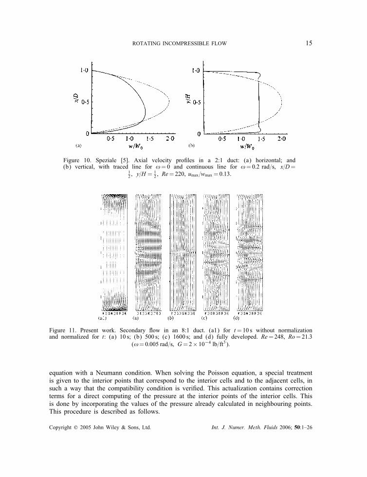
Figure 10. Speziale [5]. Axial velocity pro�les in a 2:1 duct: (a) horizontal; and(b) vertical, with traced line for !=0 and continuous line for !=0:2 rad=s; x=D=

12 ; y=H =

12 ; Re=220, umax=wmax = 0:13.

Figure 11. Present work. Secondary �ow in an 8:1 duct. (a1) for t=10 s without normalizationand normalized for t: (a) 10 s; (b) 500 s; (c) 1600 s; and (d) fully developed. Re=248, Ro=21:3

(!=0:005 rad=s; G=2× 10−4 lb=ft3).

equation with a Neumann condition. When solving the Poisson equation, a special treatmentis given to the interior points that correspond to the interior cells and to the adjacent cells, insuch a way that the compatibility condition is veri�ed. This actualization contains correctionterms for a direct computing of the pressure at the interior points of the interior cells. Thisis done by incorporating the values of the pressure already calculated in neighbouring points.This procedure is described as follows.

Copyright ? 2005 John Wiley & Sons, Ltd. Int. J. Numer. Meth. Fluids 2006; 50:1–26

16 J. R. CLAEYSSEN, E. B. ASENJO AND O. RUBIO

Figure 12. Present work. Streamlines for the secondary �ow in an 8:1 duct for t: (a) 10 s; (b) 500 s;(c) 1600 s; and (d) fully developed. Re=248, Ro=21:3 (!=0:005 rad=s; G=2× 10−4 lb=ft3).

Let u= ui; j, and P=Pi; j. The pressure is initialized by solving the equation

∇2[2]P=Dt +∇[1]:

(−uk :∇[2]uk +

1Re

∇2[2]u

k)

(48)

with a SOR method for k=0 [2].For a direct update of the variables Equation (34) is used.Let us assume that all discrete variable are known at the time k. We consider v∗ as the

velocity that would appear as the solution of Equation (34) with an absent pressure gradientby knowing the �eld uk , that is

v∗ − uk�t1

= − uk :∇[2]uk +1Re

∇2[2]u

k + F[uk] (49)

Thus

v∗= uk +�t1

(−uk :∇[2]uk +

1Re

∇2[2]u

k + F[uk])

(50)

The variable v∗ is known as pseudo-velocity [18], and does not necessarily satisfy thecontinuity equation. The Helmotz theorem [19, 20] allows to write a �nite vector �eld as thesum of a gradient of a scalar �eld with a solenoidal vector �eld, that is, with null divergence.This suggests to write v∗ as the sum of a scalar multiple of the pressure gradient at time

Copyright ? 2005 John Wiley & Sons, Ltd. Int. J. Numer. Meth. Fluids 2006; 50:1–26

ROTATING INCOMPRESSIBLE FLOW 17

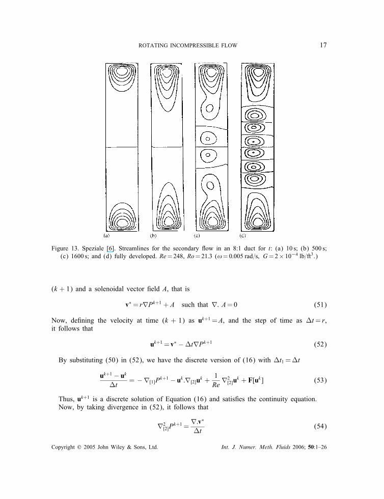
Figure 13. Speziale [6]. Streamlines for the secondary �ow in an 8:1 duct for t: (a) 10 s; (b) 500 s;(c) 1600 s; and (d) fully developed. Re=248, Ro=21:3 (!=0:005 rad=s; G=2× 10−4 lb=ft3.)

(k + 1) and a solenoidal vector �eld A, that is

v∗= r∇Pk+1 + A such that ∇: A=0 (51)

Now, de�ning the velocity at time (k + 1) as uk+1 =A, and the step of time as �t= r,it follows that

uk+1 = v∗ −�t∇Pk+1 (52)

By substituting (50) in (52), we have the discrete version of (16) with �t1 =�t

uk+1 − uk�t

= − ∇[1]Pk+1 − uk :∇[2]uk +1Re

∇2[2]u

k + F[uk] (53)

Thus, uk+1 is a discrete solution of Equation (16) and satis�es the continuity equation.Now, by taking divergence in (52), it follows that

∇2[2]P

k+1 =∇:v∗�t

(54)

Copyright ? 2005 John Wiley & Sons, Ltd. Int. J. Numer. Meth. Fluids 2006; 50:1–26

18 J. R. CLAEYSSEN, E. B. ASENJO AND O. RUBIO

Figure 14. Present work. Axial velocity pro�les in an 8:1 duct: (a) horizontal; and (b)vertical. Traced lines for !=0 and continuous lines for !=0:005 rad=s; Re=248.

Here Qf=Q=0:9290; umax=wmax = 0:0287.

Figure 15. Speziale [6]. Axial velocity pro�les in an 8:1 duct: (a) horizontal; and (b) vertical. Tracedlines for !=0 and continuous lines for !=0:005 rad=s; Re=248. Qf=Q=0:924; x=D= 1

2 ; y=H =12.

Copyright ? 2005 John Wiley & Sons, Ltd. Int. J. Numer. Meth. Fluids 2006; 50:1–26

ROTATING INCOMPRESSIBLE FLOW 19

Figure 16. Present work. (a) Pressure �eld; (b) contours; (c) horizontal pro�le for y=D=4; and (d)vertical pro�le for x=D=0:5, in an 8:1 duct. Re=248; C=0:0569; Ro=21:3.

With the substitution of (50) in (54), we arrive to the following discrete equation for thepressure at the level time (k + 1)

∇2[2]P

k+1 =∇:vk�t

+∇[1]:(

−uk :∇[2]uk +1Re

∇2[2]u

k + F[uk])

=∇:Uk +Dkt (55)

Copyright ? 2005 John Wiley & Sons, Ltd. Int. J. Numer. Meth. Fluids 2006; 50:1–26

20 J. R. CLAEYSSEN, E. B. ASENJO AND O. RUBIO

Figure 17. Present work. Streamlines for the secondary �ow in an 8:1 duct for t: (a) 1 s; (b) 25 s;(c) 50 s; and (d) fully developed. Re=171; Ro=0:3674 (!=0:2 rad=s; G=2× 10−4 lb=ft3).

The �ctitious values that appear in the discretization of the Neumann condition (44)–(47),are calculated through the following equations:

Pk+10; j = Pk1; j − hUk

0; j ; j=1; : : : ; M (56)

Pk+1N−1; j = PkN; j + hU

kN; j; j=1; : : : ; M (57)

Pk+1i;0 = Pki;1 − hV ki;0; i=1; : : : ; N (58)

Pk+1i;M+1 = Pki;M − hV ki;M ; i=1; : : : ; N (59)

For the interior points, the pressure �eld is updated by solving Equation (55) with theincorporation of values already determined, that is, we consider the one step scheme forcomputing the pressure �eld

Pk+1i; j =14 (P

k+1i; j−1 + P

k+1i−1; j + P

ki+1; j + P

ki; j+1 + h

2∇[1]Uk + h2Dkt ) (60)

where �x=�y= h.

Copyright ? 2005 John Wiley & Sons, Ltd. Int. J. Numer. Meth. Fluids 2006; 50:1–26

ROTATING INCOMPRESSIBLE FLOW 21

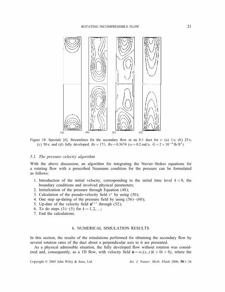
Figure 18. Speziale [6]. Streamlines for the secondary �ow in an 8:1 duct for t: (a) 1 s; (b) 25 s;(c) 50 s; and (d) fully developed. Re=171; Ro=0:3674 (!=0:2 rad=s; G=2× 10−4 lb=ft3).

5.1. The pressure–velocity algorithm

With the above discussion, an algorithm for integrating the Navier–Stokes equations fora rotating �ow with a prescribed Neumann condition for the pressure can be formulatedas follows:

1. Introduction of the initial velocity, corresponding to the initial time level k=0, theboundary conditions and involved physical parameters;

2. Initialization of the pressure through Equation (48);3. Calculation of the pseudo-velocity �eld v∗ by using (50);4. One step up-dating of the pressure �eld by using (56)–(60);5. Up-date of the velocity �eld uk+1 through (52);6. To do steps (3)–(5) for k=1; 2; : : :;7. End the calculations.

6. NUMERICAL SIMULATION RESULTS

In this section, the results of the simulations performed for obtaining the secondary �ow byseveral rotation rates of the duct about a perpendicular axis to it are presented.As a physical admissible situation, the fully developed �ow without rotation was consid-

ered and, consequently, as a 1D �ow, with velocity �eld u=w1(x; y)k + 0i + 0j, where the

Copyright ? 2005 John Wiley & Sons, Ltd. Int. J. Numer. Meth. Fluids 2006; 50:1–26

22 J. R. CLAEYSSEN, E. B. ASENJO AND O. RUBIO

Figure 19. Present work. Axial velocity pro�les in an 8:1 duct: (a) horizontal; and (b) vertical. Tracedlines for !=0 and continuous lines for !=0:2 rad=s; Re=171. Here Qf=Q=0:6603; umax=wmax = 0:1529.

Figure 20. Speziale [6]. Axial velocity pro�les in an 8:1 duct: (a) horizontal; and (b) vertical. Tracedlines for !=0 and continuous lines for !=0:2 rad=s; Re=171. Qf=Q=0:636; x=D= 1

2 ; y=H =12.

component w1 is determined by solving the Poisson equation

−�w1 =ReC (61)

Copyright ? 2005 John Wiley & Sons, Ltd. Int. J. Numer. Meth. Fluids 2006; 50:1–26

ROTATING INCOMPRESSIBLE FLOW 23

subject to a non-slip boundary condition w=0 on �. Thus, w1 corresponds to a classicalquasi-parabolic pro�le.Then, in an instant that can be de�ned as t=0, an impulsive angular velocity ! was

applied. This allows to consider the initial velocity �eld conditions

u(0)= v(0)=0 and w(0)=w1

At the walls of the duct, the conditions were prescribed

u=0; v=0; w=0

For the non-dimensional scaling, the mean velocity of the principal fully developed �ow W0

was employed as velocity scale. The angular velocity ! and the longitudinal pressure gradient−G turn out control parameters for a �xed viscosity �=1:1× 10−5 ft2=s, corresponding towater at an environment mean temperature, and the speci�c mass �=1:936 slugs=ft3. Theproblem was considered of small scale, because the characteristic length of a duct was thewidth of the traverse section D=1:92 in. The characteristic velocity was chosen as the meanvalue of the main �ow fully developed, consequently, the Reynolds number and the Rossbynumber were calculated only after the simulation.A comparison of results was done with the ones obtained by Speziale [5, 6] who employed

the vorticity-divergence formulation in contrast with the primitive variables formulation em-ployed in this work.The simulations were performed for ducts with an aspect ratio 2:1 and ducts with an aspect

ratio of 8:1. In the �rst case, a uniform grid of 32× 64 points where �x=�y=0:005 ft wasconsidered. For the duct of ratio 8:1 a grid of 16× 128 points, where �x=�y=0:01 ft wasconsidered. The stability criteria was the usual one, that is, by a superposition of the Courantand Neumann conditions [6]. More speci�cally, �t should satisfy the condition

�t6[2Re

(1�x2

+1�y2

)+umax�x

+vmax�y

]−1(62)

where umax and vmax are the maximum values of the transversal velocity components.In what follows, results are exhibited for a transversal section with aspect ratio 2:1.Figure 2 corresponds to the secondary �ow, obtained in this work, for Re=279, non-

dimensional longitudinal pressure gradient constant C=0:1345 (G=6× 10−4 lb=ft3) andRossby number Ro=1:2 (which corresponds to an angular velocity !=0:1 rad=s). Here,we observe that, in addition to the main vortices, two secondary vortices appear in the meansection of the duct. This phenomena is similar to the one that occurs with curved ducts withrectangular section [7]. In order to e�ects of comparison, in Figure 3 the correspondents resultsof Speziale [5] are presented.In the work of Speziale, the pressure was not calculated within the vorticity-divergence

formulation. In this work, the primitive variables formulation is employed and some resultsfor the pressure are obtained. This is illustrated in Figure 4, where the pressure �eld, thecontour lines and the pro�les of the central lines of the transverse section are presented.Considering the pressure �eld, it is observed that in the side more near to the axis of rotation,

Copyright ? 2005 John Wiley & Sons, Ltd. Int. J. Numer. Meth. Fluids 2006; 50:1–26

24 J. R. CLAEYSSEN, E. B. ASENJO AND O. RUBIO

called the side of the pressure, the pressure is higher if compared to the opposite side (thesuction side).Figure 5 (present work) and Figure 6 (results of Speziale [5]) present a comparison of

the longitudinal velocity pro�les, at the horizontal and vertical lines, placed in the centre ofthe transverse section. The trace lines correspond to the initial longitudinal velocity pro�les(without rotation e�ect, !=0). The continuous lines are the fully developed velocity pro�lesdue to the e�ect of rotation (!=0:1 rad=s). It is observed, also, that there is an asymmetryof the longitudinal fully developed velocity pro�les in relation to the initial pro�le, existinga deviation of the maximum of the pro�le in the direction to the side of higher pressure.It is clear that a rotation generates a loss of the �owrate in the longitudinal direction in

relation to the ratio of the �owrate that is able to carry the primary �ow in the absenceof rotation. This ratio is de�ned by Qf=Q, where Qf is the end �owrate and Q is the ini-tial �owrate. In this work Qf=Q=0:5429 and the ratio of the maximum values among thehorizontal and the longitudinal components of the velocity �eld is given by umax=wmax =0:15.For a greater angular velocity such as !=0:2 rad=s, that is Ro=0:48, Re=220 and

C=0:2296, the secondary �ow, before reaching the state of fully developed, has periodsof instability as it can be observed in Figure 7.In Figure 7, we observe that the secondary vortices at the centre section are moved to the

inferior and superior ends. However, in the period of time t=40 s until t=60 s (Figures 7 (b)–(g)), it can be observed that four vortices at the centre appear, two of which are moved tothe ends, and the other two are dissipated at the same centre, when it was reaching the fullydeveloped �ow (Figure 7(h)). Approximately at t=500 s, the �ow is able to stabilize in twocounter-rotating vortices. The results obtained in this work (Figure 7(h)) can be comparedwith the ones obtained by Speziale [5] (Figure 8).Figure 9 (present work) and Figure 10 (results of Speziale [5]) illustrate comparisons of

the longitudinal velocity pro�les of the fully developed �ow.Now we consider a transverse section with aspect ratio 8:1. Figures 11 and 12, exhibit the

secondary �ow, obtained in this work, for Ro=21:3, !=0:005 rad=s. It can be observed that,in the centre of the left side and for time t=10, there is a small disorder, consequence of therotation. Although, they have a neglecting presence, as one can see, the streamlines do notcapture this fact. In Figure 11(a1), the velocity �eld without normalization is presented fort=10. Here we cannot observe the phenomena exhibit in Figure 11(a), that is, the velocity�eld, in this portion of the transversal section, is smaller than the �elds that appear in theinferior and superior faces. It can be said that the normalized velocity �eld exhibits moreinformation of what happens in the other portions of the solution domain. This is one of theadvantages of working in primitive variables.In Figure 12 it is observed too that the secondary �ow initially assumes a double vortex

con�guration where each vortex, whose size is the order of the width of the channel, isslightly compressed against the horizontal wall of the channel to which it is adjacent. Then,the stretched double vortex secondary �ow becomes unstable so that it becomes a doublevortex secondary �ow combined with roll-cells in the interior of the channel. In Figure 13the correspondents results of Speziale [6] are presented.The present algorithm allows to determine quicker the secondary �ow. For instance, a

similar structure to the one obtained by Speziale [6] in 1600 s, is obtained by the presentalgorithm in 750 s. The fully developed �ow is qualitatively the same as the one obtained bySpeziale.

Copyright ? 2005 John Wiley & Sons, Ltd. Int. J. Numer. Meth. Fluids 2006; 50:1–26

ROTATING INCOMPRESSIBLE FLOW 25

Figure 14 (present work) and Figure 15 (results of Speziale [6]), exhibit a comparisonof the longitudinal velocity pro�les. The initial one, without rotation (!=0) with a tracedline, and the fully developed (!=0:005 rad=s) with a continuous line, for the �owrate thatdecreases in approximately 7:6%. For the same parameters, results, obtained in this work, forthe pressure in a state fully developed are given in Figure 16.For a greater angular velocity such as !=0:2 rad=s, that is, Ro=0:3674; Re=171 and

C=0:1196 (G=2× 10−4 lb=ft3), the secondary �ow restabilizes to a stretched double vortexcon�guration, as it can be observed in Figure 17(d) (present work) and in Figure 18(d)(results of Speziale [6]). The corresponding velocity pro�les are shown in Figure 19 (presentwork) and in Figure 20 (results of Speziale [6]). For this faster rotating channel, there is areduction in the �owrate of approximately 37%.We should mention that all the results showed here, for ducts with aspect ratio 2:1 and

8:1, are in good agreement with those obtained by Speziale [5, 6].

7. CONCLUSIONS

A numerical study of the internal �ow of an incompressible viscous �uid in a rectangularduct subject to a rotation force has been developed. Finite di�erences in primitive variablesin a staggered grid with a Neumann condition [1] for the pressure were employed.Numerical simulations were made for ducts with aspect ratios 2:1 and 8:1, for a wide variety

of Reynolds numbers and rotation rates, by using a direct velocity–pressure algorithm [2]. Thisalgorithm solves without any iteration the Poisson equation for the pressure. This equation istime dependent due to the incorporation of the velocity �eld through the Neumann conditionfor the pressure.The results obtained for a duct of aspect ratio 2:1, show the breakdown of the double-

vortex secondary �ow as well as their e�ects in the axial �ow. For Re=279 and rotationrate !=0:1rad=s (Ro=1:2) it is observed that the secondary �ow starts with a double-vortexcon�guration and then breaks down in a con�guration of four counter-rotating vortices that arenon-symmetric with respect to the central vertical line of the duct (Figure 2(d)). The resultantsecondary �ow is very similar to those obtained by Chen et al. [7] for curved rectangulardutos. When the angular speed of the duct is increased for !=0:2 rad=s (Re=220 andRo=0:48) it is observed that the subsidiary counter-rotating vortices pair that were on the sideof the high pressure of the duct (Figure 2(d)) disappear and the secondary �ow restabilizesto a slightly asymmetric double-vortex con�guration as shown in Figure 7(h).For a duto 8:1 with Re=248 and !=0:005rad=s (Ro=21:3), it is observed that the double

secondary vortex initially obtained (Figure 12(a)) is replaced with the double vortex secondary�ow combined with roll-cells in the interior of the channel (Figure 12(d)). When the angularvelocity of the duct is increased to !=0:2 rad=s (Ro=0:3674 and Re=171), the secondary�ow restabilizes to the stretched double vortex con�guration (Figure 17(d)).The simulations for the ducts of aspect ratio 2:1 and 8:1 were compared with the existent

solutions [5, 6], showing a very good agreement.The numerical scheme developed in this work for a rotating �ow could be employed in

connection with non-Newtonian �uids and mixed convection problems. They are matter of afuture work of the authors.

Copyright ? 2005 John Wiley & Sons, Ltd. Int. J. Numer. Meth. Fluids 2006; 50:1–26

26 J. R. CLAEYSSEN, E. B. ASENJO AND O. RUBIO

REFERENCES

1. Gresho PM, Sani RL. On pressure boundary conditions for the incompressible Navier–Stokes equations.International Journal for Numerical Methods in Fluids 1987; 7:1111–1145.

2. Claeyssen JR, Bravo E, Platte R. Simulation in primitive variables of incompressible �ow with pressure Neumanncondition. International Journal for Numerical Methods in Fluids 1999; 30:1009–1026.

3. Harlow FH, Welch JE. Numerical calculation of time dependent viscous incompressible �ow of �uid with freesurface. Physics of Fluids 1965; 8:2182–2189.

4. Robertson AM. On viscous �ow in curved pipes of non-uniform cross-section. International Journal forNumerical Methods in Fluids 1996; 22:771–798.

5. Speziale CG. Numerical study of viscous �ow in rotating rectangular ducts. Journal of Fluid Mechanics 1982;122:251–271.

6. Speziale CG. Numerical Solution of Rotating Internal Flows. Lectures in Applied Mathematics, vol. 22.American Mathematical Society: Providence, RI, 1985; 261–288.

7. Chen HB, Nandakumar K, Finlay WH, Ku HC. Three-dimensional viscous �ow through rotating channel: apseudospectral matrix method approach. International Journal for Numerical Methods in Fluids 1996; 23:379–396.

8. Yang Z. Large eddy simulation of fully developed turbulent �ow in a rotating pipe. International Journal forNumerical Methods in Fluids 2000; 33:681–694.

9. Govatsos PA, Papantonis DE. A characteristic based method for the calculation of three-dimensionalincompressible, turbulent and steady �ows in hydraulic turbomachines and installations. International Journalfor Numerical Methods in Fluids 2000; 34:1–30.

10. Hart JE. Instability and secondary motion in a rotating channel �ow. Journal of Fluid Mechanics 1971; 45:341–351.

11. Ladyzhenskaya O. The Mathematical Theory of Viscous Incompressible Flow. Gordon and Breach: New York,1969.

12. Sheu TWH, Wang MMT, Tsai SF. Pressure boundary condition for a segregated approach to solvingincompressible Navier–Stokes equations. Numerical Heat Transfer, Part B 1998; 34:457–467.

13. Roache PJ. Computational Fluid Dynamics. Hermosa Publishers: Albuquerque, NM, 1982.14. Ames WF. Numerical Methods for Partial Di�erential Equations (3rd edn). Academic Press: New York, 1992.15. Ferziger JH, Peric M. Computational Methods for Fluid Dynamics (2nd edn). Springer: Berlin, 1999.16. Abdallah S. Numerical solutions for the pressure Poisson equation with Neumann boundary conditions using a

non-staggered grid. Journal of Computational Physics 1987; 70:182–192.17. Alfrink BJ. On the Neumann problem for the pressure in a Navier–Stokes model. Proceedings of the 2nd

International Conference on Numerical Methods in Laminar and Turbulent Flow, Venice, 1981; 389–399.18. Nonino C, Comini G. An equal-order velocity–pressure algorithm for incompressible thermal �ows. Part 1:

formulation. Numerical Heat Transfer, Part B 1997; 32:1–15.19. Morse PM, Feschbach H. Methods of Theoretical Physics, Part I. McGraw-Hill: New York, 1953.20. Temam R. Navier–Stokes Equations (3rd edn). North-Holland: Amsterdam, 1985.

Copyright ? 2005 John Wiley & Sons, Ltd. Int. J. Numer. Meth. Fluids 2006; 50:1–26