DYNAMIC ANALYSIS OF ROTATING SYSTEMS INCLUDING ...
147
Eerik Sikanen DYNAMIC ANALYSIS OF ROTATING SYSTEMS INCLUDING CONTACT AND THERMAL-INDUCED EFFECTS Acta Universitatis Lappeenrantaensis 820
-
Upload
khangminh22 -
Category
Documents
-
view
2 -
download
0
Transcript of DYNAMIC ANALYSIS OF ROTATING SYSTEMS INCLUDING ...
Eerik Sikanen
DYNAMIC ANALYSIS OF ROTATING SYSTEMSINCLUDING CONTACT AND THERMAL-INDUCEDEFFECTS
Acta Universitatis Lappeenrantaensis
820
Acta Universitatis Lappeenrantaensis
820
ISBN 978-952-335-284-1 ISBN 978-952-335-285-8 (PDF)ISSN-L 1456-4491ISSN 1456-4491Lappeenranta 2018

Eerik Sikanen
DYNAMIC ANALYSIS OF ROTATING SYSTEMSINCLUDING CONTACT AND THERMAL-INDUCEDEFFECTS
Acta Universitatis Lappeenrantaensis 820
Thesis for the degree of Doctor of Science (Technology) to be presented with due permission for public examination and criticism in Auditorium 2303 at Lappeenranta University of Technology, Lappeenranta, Finland on the 16th of November, 2018, at noon.

Supervisors Professor Jussi Sopanen
Reviewers
L UT School of Energy Systems Lappeenranta University of Technology Finland
D.Sc. (Tech.) Janne E. HeikkinenL UT School of Energy SystemsLappeenranta University of TechnologyFinland
Professor Reijo Kouhia Department of Civil Engineering Tampere University of Technology Finland
Associate Professor Jani Romanoff Department of Mechanical Engineering Aalto University Finland
Opponents Professor Reijo Kouhia Department of Civil Engineering Tampere University of Technology Finland
D.Sc. (Tech.) Erkki LanttoSulzer Pumps Finland OyFinland
ISBN 978-952-335-284-1 ISBN 978-952-335-285-8 (PDF)
ISSN-L 1456-4491 ISSN 1456-4491
Lappeenranta University of Technology Yliopistopaino 2018


Acknowledgements
I would like to thank my supervisors Professor Jussi Sopanen and D.Sc. (Tech.)Janne E. Heikkinen for providing me an opportunity to join the internationalresearch group and to pursue my doctoral degree.
I have had an opportunity to work for many multidisciplinary projects related tohigh-speed rotating electrical machines during my doctoral studies. Therefore,in addition to Professor Sopanen’s research group, I would like to thank D.Sc.(Tech.) Janne Nerg and D.Sc. (Tech.) Rafał Piotr Jastrzebski regarding onelectromechanical research opportunities. Also, I would like to thank ProfessorJari Backman and L.Sc. (Tech.) Juha Honkatukia regarding on heat transferand fluid-structure interaction studies related to multidisciplinary research onhigh-speed rotating electrical machines.
Lappeenranta, November 2018
Eerik Sikanen


Contents
1 Introduction 191.1 Motivation . . . . . . . . . . . . . . . . . . . . . . . . . . . . . . . 201.2 Literature survey . . . . . . . . . . . . . . . . . . . . . . . . . . . . 21
1.2.1 Rotor dynamics modeling using finite element method . . . 211.2.2 Thermal stress modeling using finite element method . . . . 25
1.3 Objectives and scientific contribution . . . . . . . . . . . . . . . . . 261.4 Published articles . . . . . . . . . . . . . . . . . . . . . . . . . . . . 28
2 Finite element modeling of rotating structures 312.1 Finite element method for 3D solids . . . . . . . . . . . . . . . . . 34
2.1.1 Introduction to three-dimensional elements . . . . . . . . . 342.1.2 Energy principle for formulating element matrices . . . . . 372.1.3 Heat transfer theory . . . . . . . . . . . . . . . . . . . . . . 452.1.4 Finite element method for three-dimensional heat transfer . 46
2.2 Constraint equations and contact modeling . . . . . . . . . . . . . 482.2.1 Master-slave method . . . . . . . . . . . . . . . . . . . . . . 492.2.2 Penalty function method . . . . . . . . . . . . . . . . . . . . 532.2.3 Lagrangian multiplier method . . . . . . . . . . . . . . . . . 542.2.4 Trial force method . . . . . . . . . . . . . . . . . . . . . . . 562.2.5 Use of constraint equations for contact modeling . . . . . . 592.2.6 Summary on constraint equations . . . . . . . . . . . . . . . 61
2.3 Solution methods . . . . . . . . . . . . . . . . . . . . . . . . . . . . 622.3.1 Undamped and damped eigenvalue problem . . . . . . . . . 622.3.2 Coupled thermal mechanical analysis . . . . . . . . . . . . . 652.3.3 Fundamentals of fatigue life calculation . . . . . . . . . . . 672.3.4 Transient analysis of rotor dropdown event . . . . . . . . . 67
3 Studies of rotating structures 713.1 Rotor dropdown simulation . . . . . . . . . . . . . . . . . . . . . . 71
3.1.1 Dropdown simulation of an AMB-supported rotor . . . . . 723.1.2 Rotor stresses during dropdown event . . . . . . . . . . . . 753.1.3 Discussion . . . . . . . . . . . . . . . . . . . . . . . . . . . . 76
3.2 Bearing stress simulation . . . . . . . . . . . . . . . . . . . . . . . 793.2.1 Stress in a backup bearing during dropdown . . . . . . . . . 813.2.2 Discussion . . . . . . . . . . . . . . . . . . . . . . . . . . . . 84
3.3 Rotors with internal contacts . . . . . . . . . . . . . . . . . . . . . 863.3.1 Experimental results of test shaft assembly . . . . . . . . . 863.3.2 Numerical results of test shaft assembly . . . . . . . . . . . 883.3.3 Discussion of verification of shrink fit joint modeling . . . . 893.3.4 Accuracy of contact modeling . . . . . . . . . . . . . . . . . 903.3.5 Discussion of use of constraint equations . . . . . . . . . . . 923.3.6 Conical impeller assembly . . . . . . . . . . . . . . . . . . . 943.3.7 Effect of geometric nonlinearities to the critical speeds . . . 99
3.4 Thermal stress studies . . . . . . . . . . . . . . . . . . . . . . . . . 1013.4.1 Thermal stress analysis of traction motor . . . . . . . . . . 101

3.4.2 Thermal stress results . . . . . . . . . . . . . . . . . . . . . 1053.4.3 Discussion . . . . . . . . . . . . . . . . . . . . . . . . . . . . 108
4 Conclusions 1134.1 Summary of solution methods . . . . . . . . . . . . . . . . . . . . . 1134.2 Rotor dropdown studies . . . . . . . . . . . . . . . . . . . . . . . . 1144.3 Bearing stress studies . . . . . . . . . . . . . . . . . . . . . . . . . 1154.4 Summary of internal contact studies . . . . . . . . . . . . . . . . . 1154.5 Thermal stress studies . . . . . . . . . . . . . . . . . . . . . . . . . 1164.6 Future work . . . . . . . . . . . . . . . . . . . . . . . . . . . . . . . 116
Bibliography 119
A Constructing element shape functions 129
B Common isoparametric elements 133
C Numerical integration 139

Symbols and abbreviations
Symbols
0 Zero matrixa Lower integration limitA State space matrixAb Bordered stiffness matrixb Upper integration limitb Vector of non-homogeneous coefficients in Lagrangian multiplier
methodbe Basquin exponent or fatigue strength exponentB Strain matrixBd Matrix of shape function derivativesBi Strain matrix of ith nodeBε Matrix containing the spatial derivatives of the element shape
functionsc Specific heat capacityC Heat capacity matrixCe Element heat capacity matrixCb Bearing damping matrixCe Elastic damping matrixCtot Total damping matrixde First time derivative of element displacement vector
˙de,i First time derivative of element displacement vector of node ide Element displacement vectordi Nodal displacement vector of node iD Matrix of material constantsDc Conductivity matrixeg Constraint errorE Elastic modulusfx Force components in global X-directionfy Force components in global Y -directionfz Force components in global Z-directionf eb Element nodal body force vectorf es Element nodal surface force vectorF Force vectorF Modified force vectorF ′c Contact force vector in the cylindrical coordinate systemF ′c,trial Trial contact force vector in the cylindrical coordinate systemF eb Element body force vector
F eg Element translational acceleration force vector
F eext Element total external force vector
F ep Element pressure force vector
F es Element surface force vector
F e∆T Element thermal expansion force vector
F eε Element strain force vector
F eΩ Element centrifugal force vector
F brg Bearing force vectorF c Contact force vector the Cartesian coordinate systemF c,trial Trial contact force vector in the Cartesian coordinate systemF ext External force vectorF tot Total force vectorF tot,shaft Total force vector of shaft bodyF tot,sleeve Total force vector of sleeve bodyFUB Unbalance force vector at constant rotational speedF α,UB Unbalance force vector due to angularFΩ Centrifugal force vectorg Gapg Vector of non-homogeneous coefficientsga Acceleration coefficient vectorgx Acceleration coefficient in global X-directiongy Acceleration coefficient in global Y -directiongz Acceleration coefficient in global Z-directionG Gyroscopic damping matrixGe Element gyroscopic damping matrixh Convection coefficienti ithiu Imaginary unitI IntegralI3 3× 3 identity matrixj jthJ JacobianJ Jacobian matrixk kthk0 Initial contact stiffnesskf Vector of multipliers for initial contact stiffnesskmax Magnitude of greatest coefficient in stiffness matrixkx Thermal conductivity coefficient in global X-directionky Thermal conductivity coefficient in global Y -directionkz Thermal conductivity coefficient in global Z-directionK Stiffness matrixK Modified stiffness matrixKeC Element heat conduction matrix
Kee Element elastic stiffness matrix
KeG Element stress-stiffening matrix
Keh Element heat convection matrix
Kassembly Stiffness matrix of assemblyKb Bearing stiffness matrixKc Contact stiffness matrixKC Heat conduction matrix

Ke Elastic stiffness matrixKe,CYL Elastic stiffness matrix applied with cylindrical constraintsKG Stress stiffening matrixKh Surface convection matrixKshaft Stiffness matrix of shaft bodyKsleeve Stiffness matrix of sleeve bodyKtot Total stiffness matrixl Number ofL LengthL Matrix of partial differential operationsm Number ofM Mass matrixMe Element mass matrixn Number ofn Outer normal to the surface of the bodynrpm Rotational speednx Outer normal to the surface of the body in global X-directionny Outer normal to the surface of the body in global Y -directionnz Outer normal to the surface of the body in global Z-directionN Number of stress cycle repetitions in totalN Shape function matrixN Vector of shape functionsN1 Shape function matrix of node 1N2 Shape function matrix of node 2Nf Number of equivalent applied stress cyclesNi Shape function of node iNi Shape function matrix of ith nodeNj Shape function matrix of jth nodeNn Shape function matrix of node np pthp Vector of monomialspp Pressure vectorpw Working precisionpx Pressure normal component in global X-directionpy Pressure normal component in global Y -directionpz Pressure normal component in global Z-directionP Power lossP Moment matrixq Heat flow vectorqs Boundary heat flow component coefficientqx Heat flow component through the unit area in global X-directionqy Heat flow component through the unit area in global Y -directionqz Heat flow component through the unit area in global Z-directionQ Internal heat generation rate per unit volumeReh Element surface convection vector
Req Element boundary heat flow vector

ReQ Element internal heat generation vector
ReT Element specified boundary temperature vector
Rh Heat convection vectorRq Boundary heat flow vectorRQ Internal heat generation vectorRT Specified boundary temperature vectorS Surface areaS0 Initial stress matrixSe Element surface areat Timeti Time of step iT TemperatureTi Temperature of node iT Transformation matrixTN First time derivative of nodal temperature vectorTd Transformation matrix containing diagonal termsTe Reference temperature for convective heat transferTg Kinetic energy due to gyroscopic effectTk Kinetic energyTm Kinetic energy of translational motionTN Nodal temperature vectorTs Surface temperatureTref Reference temperatureu Nodal displacement in global X-directionu Element displacement vectoru Modified displacement vectoru First time derivative of displacement vectorui First time derivative of nodal displacement of node i in global
X-directionu′0,s Initial displacement vector of source nodes in cylindrical
coordinatesu′0,t Initial displacement vector of target nodes in cylindrical
coordinatesu′s,i Displacement of source node i in cylindrical coordinate systemu′t,i Displacement of target node i in cylindrical coordinate systemutrial Trial displacement vector in global Cartesian coordinate systemu′trial Trial displacement vector in cylindrical coordinate systemu0 Initial displacement vectorui Nodal displacement of node i in global X-directionuj Nodal displacement of node j in global X-directionur Radial displacement in cylindrical coordinate systemushaft Displacement vector shaft bodyusleeve Displacement vector sleeve bodyutot Total displacement vectoruw Axial displacement in cylindrical coordinate systemux Nodal displacement in global X-direction

uy Nodal displacement in global Y -directionuz Nodal displacement in global Z-directionv Nodal displacement in global Y -directionvi First time derivative of nodal displacement of node i in global
Y -directionvi Nodal displacement of node i in global Y -directionV VolumeVe Element volumew Nodal displacement in global Z-directionwi First time derivative of nodal displacement of node i in global
Z-directionwi Nodal displacement of node i in global Z-directionW Penalty weightWf Work done by external forcesWi Weight coefficient iWj Weight coefficient jWk Weight coefficient kx Nodal coordinate in global X-directionx Nodal coordinate vector in fixed coordinate systemx First time derivative of nodal coordinate vectorx Second time derivative of nodal coordinate vectorxi Integration point ixi Vector of coordinates of node ixj Nodal coordinate in global X-direction of node jxj Vector of coordinates of node jxn Vector of coordinates of node nX Cartesian coordinate system axis in global X-directionX ′ Cylindrical coordinate system axis in global radial directiony Nodal coordinate in global Y -directionyi Nodal coordinate of node i in global Y -directionyj Nodal coordinate in global Y -direction of node jY Cartesian coordinate system axis in global Y -directionY ′ Cylindrical coordinate system axis in global tangential directionz Nodal coordinate in global Z-directionzci Number of repetitions in ith stress classzi Nodal coordinate of node i in global Z-directionzi Eigenvector of ith eigenmodezj Nodal coordinate of node j in global Z-directionZ Cartesian coordinate system axis in global Z-directionZ ′ Cylindrical coordinate system axis in global axial direction
Greek letters
α Thermal expansion coefficientα Vector of thermal expansion coefficients

αp Proportional coefficient for stiffness matrixαx Thermal expansion coefficient in global X-directionαy Thermal expansion coefficient in global Y -directionαz Thermal expansion coefficient in global Z-directionβ S-N curve slopeβp Proportional coefficient for mass matrixγ ′0 Vector of logical multipliersγxy Shear strain in XY -planeγxy,0 Initial shear strain in XY -planeγxz Shear strain in XZ-planeγyx Shear strain in Y X-planeγyz Shear strain in Y Z-planeγyz,0 Initial shear strain in Y Z-planeγzx Shear strain in ZX-planeγzx,0 Initial shear strain in ZX-planeγzy Shear strain in ZY -planeδrad Radial interferenceδui Distance between source and target node i∆L Change of length∆T Change of temperature∆Tn Temperature difference of node n∆u′0 Vector of initial radial distances between source–target nodes in
cylindrical coordinates∆u′trial Vector of radial distances between source–target nodes in
cylindrical coordinates after trial force evaluation∆u′trial,i Radial distances between source and target node i in cylindrical
coordinates after trial force evaluation∆σ Stress variation∆σeq Calculated equivalent stressε Strainε Strain vectorε0 Initial strain vectorεx Normal strain in X-directionεx,0 Initial normal strain in X-directionεy Normal strain in Y -directionεy,0 Initial normal strain in Y -directionεz Normal strain in Z-directionεz,0 Initial normal strain in Z-directionζ Natural coordinateζi Integration point iζk Integration point kζl Natural coordinate ζ of node lη Natural coordinateηi Integration point iηj Integration point jηl Natural coordinate η of node l

θ Rotational degree of freedomθx First time derivative of nodal rotation around global X-axisθy First time derivative of nodal rotation around global Y -axisθz First time derivative of nodal rotation around global Z-axisθx Nodal rotation around global X-axisθy Nodal rotation around global Y -axisθz Nodal rotation around global Z-axisκ Number of the rainflow stress classesλ Lagrangian multiplierλ Vector of Lagrangian multipliersλii Imaginary part of eigenvalue iλri Real part of eigenvalue iλi Eigenvalue of ith eigenmodeν Poisson’s ratioξ Natural coordinateξdi Damping ratio of ith eigenmodeξi Integration point iξl Natural coordinate ξ of node lΠ Strain energyρ Material densityσ Element stress vectorσ′f Fatigue strength coefficientσbrg Bearing stress vectorσeq Equivalent stressσmax Maximum stressσrotor Rotor stress vectorσx Normal stress in X-directionσy Normal stress in Y -directionσz Normal stress in Z-directionτ Torqueτxy Shear stress in XY -planeτxy,0 Initial shear stress in XY -planeτxz Shear stress in XZ-planeτyx Shear stress in Y X-planeτyz Shear stress in Y Z-planeτyz,0 Initial shear stress in Y Z-planeτzx Shear stress in ZX-planeτzx,0 Initial shear stress in ZX-planeτzy Shear stress in ZY -planeωd,i Damped natural frequency of ith eigenmodeωn,i Undamped natural frequency of ith eigenmodeωx Angular velocity around global X-axisωy Angular velocity around global Y -axisωz Angular velocity around global Z-axisΩ Rotational speedΩ Rotational speed matrix

Ω Angular acceleration
Abbreviations
1D One-dimensional2D Two-dimensional3D Three-dimensionalAMB Active magnetic bearingBM Bending modeBW Backward whirlCAD Computer-aided designCS Critical speedDOF Degree of freedomEMA Experimental modal analysisFE Finite elementFEA Finite element analysisFEM Finite element methodFW Forward whirlMPC Multipoint constraintPMSM Permanent magnet synchronous motor
Chapter 1Introduction
Rotating machines are used in various processes, such as transforming energy fromone form into another. Commonly, electrical energy is transformed into mechanicalrotational motion or vice versa. As the rotational machines are developed, theyget more optimized and efficient. Traditional industrial electrical motor-drivenblowers use a low-speed electric motor and a transmission to increase the rotationalspeed for the blower. By getting rid of the transmission – typically the mainsource of unwanted frictional losses – as well as designing the electrical motor forincreased rotational speed applications resulting in a direct-driven system, thetotal efficiency of the system can be increased. This type of machine is generallycalled a high-speed machine. The benefits of proceeding towards high-speedtechnology are generally the smaller size and weight of the rotating machines.Also, a greater power density and better efficiency of fluid flow process in variousindustrial process components such as high-speed electrical fans, blowers andpumps, are achieved.
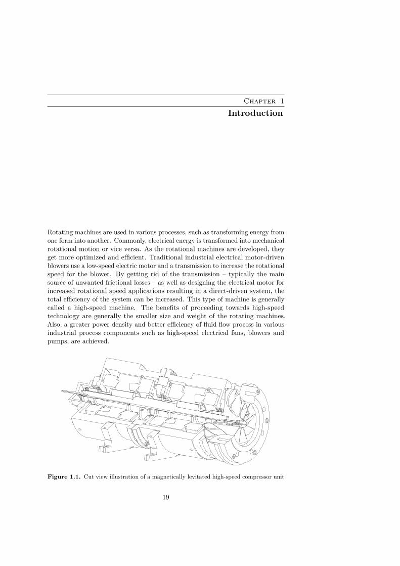
Figure 1.1. Cut view illustration of a magnetically levitated high-speed compressor unit
19

20 1 Introduction
Modern high-speed rotating machines consist of multiple parts. A cut view of amagnetically levitated high-speed compressor unit is shown in Figure 1.1. A rotorof a high-speed motor has typically one main shaft component and a number ofother components, such as impellers and lamination stacks, depending on themotor-rotor type and bearing solution, attached on the shaft. Quite often, theseparts are attached using a frictional joint. These joints are capable of causingnonlinearities in the rotating structure dynamics.
A high-speed rotating operation is that which, from the mechanical point of view,could be regarded as a rotating operation having the peripheral velocity of therotation part high enough, typically above 150 m/s [85]. The angular velocity orrevolutions per minute is a relative quantity, and thus should not be consideredas a definition for high-speed. The strength of material is typically the limitingfactor for high-speed machine design. Often, in rotating high-speed machines, thestrength of the material used sets the upper limit for the rotational speed.
In addition to loads induced by high-speed rotation, heat loads induced bypower loss of an electrical machine should be taken into account in the form ofthermal stress. This doctoral dissertation examines high-speed rotating structures,commonly referred as rotors. The research on these rotors – rotor assemblies asmore detailed in most cases – is a special field and a part of structural dynamicsreferred to as rotor dynamics. The main tool used in this dissertation is the three-dimensional solid finite element method, as part of the finite element method usedwithin the field of structural engineering.
1.1 Motivation
The interest for programming 3D solid finite element problems arises from thecapability to use customized contact models and solution routines for coupledanalyses, thus extending the capabilities of commercial FE software. Coupledanalysis can be, for example, a combined thermal structural stress analysis: in thefirst phase, the temperature state is solved and used as an input for the secondphase. The solved temperature distribution is applied as an initial thermal strain,thus contributing the total stresses in a form of thermal stress.
Another example of coupled analysis can be a static structural–modal analysis, orpre-stressed modal analysis, in order to include the effect of external structuralloads in the modal analysis. An eigenvalue problem cannot handle structuralloads directly: thus, a static structural analysis is performed to solve the stressstate of the structure. The solved stress state can be included into the eigenvalueproblem as a pre-stress state by utilizing the stress-stiffening effect; an additionalstiffness matrix to represent the stress-stiffening effect can be formed using thepre-solved stress state of the structure.
Many commercial FE software can be used to solve coupled field problems asdescribed above. Even so, performing an analysis using self-programmed solutionroutines and finite elements may be required in certain cases if commercial softwaredoes not support a particular analysis routine. For example, a control design for
1.2 Literature survey 21
active magnetic bearing using a 3D solid element rotor model having multiplecontact and possible contact-induced disturbances.
1.2 Literature survey
Rotor dynamics analysis is an important part of the design process in high-speed machinery design. The traditional one-dimensional (1D) Timoshenko beamelement approach in rotor dynamics can represent only flexible shafts, while thedisks and impellers are modeled as rigid mass points. [74, 73, 34] Although thiselement type can have degrees of freedom (DOFs) in up to three dimensions, itis commonly referred as 1D element because of the element formulation. Beamelements are actively used because of their benefits: a low number of degrees offreedom is required to represent a full rotor model. Because of a low numberof DOFs, transient simulation for solving nonlinear problems is fast and designoptimization is easy to implement. These 1D elements do not normally takeinto account the deformation of the shaft cross section. In certain rotatingmachinery applications, the effect of deformable shaft cross sections for flexibledisks and turbine blades are required to be included into the simulation model.These features enable the inclusion of the stress-stiffening effect, meaning thatthe total stiffness of the rotor assembly is affected by the internal stress of thecomponent. [32] These effects can be included when using two-dimensional (2D)axisymmetric harmonic or three-dimensional (3D) solid finite elements. [35, 69, 80]The use of a 2D element is typically limited to axisymmetric structures andaxisymmetric loads, whereas 3D elements in practice can be used to describe anyrotating structure. In addition, high-fidelity coupled field analyses become easierto implement when using the same solid finite element mesh for various analyses.
The use of three-dimensional solid finite elements in rotor dynamic analysis allowsthe inclusion of nonlinear contact behavior in the study of a rotor assembly.Modern complex rotor assemblies used in high-speed rotating machinery caninclude multiple parts with various types of joints as shown in Figure 1.1. Thecontact modeling and inclusion of frictional joint-based excitations are features thathave been challenging to include in the analysis when using the conventional beamelement approach. The use of axisymmetric elements will limit the capabilitiesto model arbitrary external loads and load directions. Therefore, the use of 3Dsolid finite element approach is a solution for the detailed modeling of contact-based phenomena. Additional phenomena, such as centrifugal stiffening or stressstiffening, will yield further accuracy in the finite element solution. Centrifugalstiffening is derived from the centrifugal load only; whereas stress stiffening isderived, not only from centrifugal load, but from all external loads being takeninto consideration.
1.2.1 Rotor dynamics modeling using finite element method
In certain applications, such as turbines, fans and pumps, high-speed motors can bemore suitable due to process-based demands than lower speed motors which rotate

22 1 Introduction
at the power grid frequency, since high-speed motors can operate without the needfor transmission. In some applications, mechanical bearings are not suitable forsupporting the rotor of high-speed electrical motors, because mechanical bearingsrequire lubrication, can wear out, and the occurring vibrations, as a result ofrotor-bearing contact, could be critical. Active magnetic bearings (AMBs) areoften seen as the answer to the demand of supporting the high-speed rotor, sincethey do not have mechanical contact, and they are also oil-free. In addition, theefficiency of an AMB-supported rotor is better than that of a conventional rollingelement bearing-supported rotor, as the system lacks contact-induced friction.Furthermore, the stiffness of AMBs can be adjusted for recovering possible criticalspeed or other disturbance, and the rotor lateral position and axial clearances canbe adjusted if so desired.However, a failure can occur in the AMB system, and for this reason the backupbearings – typically a set of rolling element bearings – are used to support therotor in any eventual abnormal operation. In practice, this means that, due tothe backup bearings, possible contact is avoided between the stator of the electricmotor or stator of the AMBs and the rotating rotor. The AMB-supported rotordropdown event has been clarified extensively. For instance, in studied by Ishiiand Kirk [40], Zeng [97] and Cole et al. [19] the dropdown event between the rotorand bearing is examined, covering the views of modeling the stiffness, dampingand friction. They studied the dynamic behavior of a rolling element backupbearing after rotor impact and stated that for minimizing the energy dissipationin the inner ring of the bearing, it should be allowed to accelerate as rapidly aspossible in order to minimize the friction-induced whirling of the rotor.In previous research, significant research has been performed in the studyingof AMB-supported rotor deflections. Schmied and Pradetto [88] did one of thefirst studies in the field of the contact event between AMB-supported rotor andbackup bearings. In the recent years, the rotor deflections have been investigatedin normal runs of the AMB-supported rotor, as in Jalali et al. [42] and Stimac etal. [93]. In Jalali et al., the theoretical and experimental results from a high-speedrotor are found to be in good agreement. The rotating system is studied by meansof the Campbell diagram, and critical speeds and operational deflection shapesare obtained. In Stimac et al., the finite element method based on Bernoulli-Eulerbeam element theory is used for the rotor model. Frequency responses of thesystem model with amplitudes in rotor lateral displacements are verified by meansof measured results. Zhou et al. [100] investigated cracked shafts supported withAMBs. The contact region of even a slight crack can open or close due to thenormal rotation of the shaft and can thereby produce an excited dynamic system.Therefore, it is critical to examine rotor stresses, as the rotor stress state mayinitiate the rotor cracks. Nevertheless, the stresses that arise in the rotor itselfhave not been examined in the literature.A limited number of publications can be found that particularly focus on bearinglife and the stress analysis of backup bearings. Stress and life time are importantissues for engineers designing backup bearings, especially since the rolling elementin backup bearing applications undergoes exceptional loading. Sun [94] estimated

1.2 Literature survey 23
the fatigue life of the backup bearing. He evaluated the Hertzian contact stressesand implemented Lundberg-Palmgren method to approximate the fatigue life ofthe bearing. The Lundberg-Palmgren method is applicable only for steady stateloading conditions, while the loading of backup bearing is varies with regard to thetime period. After a few years, Lee and Palazzolo [55] applied rainflow analysis toconsider the time-dependent stress in evaluating the fatigue life of backup bearing.
The use of beam element-based modeling for transient problems, such as rotordropdown event or other purposes such as solving stress history of backup bearing,has proven to be useful – and is still in active use, despite its limitations withregard to the detailed modeling capabilities of the rotor geometry.
General 3D rotor dynamics modeling is discussed in Jalali et al. [42], wherethe modal results of beam and 3D modeling approaches are compared againstexperimentally measured results. In Kumar et al. [53], an aircraft engine strengthand life time analysis is given, where transient forces including gyroscopic loadsduring maneuvers are included. For the life time analysis, a flight cycle profileis used. In [69] is given a general 3D theory for rotor dynamics modeling usingboth the rotating frame of reference approach, which includes the Coriolis andspin softening effects, and the fixed frame of reference approach.
A multistage rotor system of a high-speed pump is investigated by Jammi [43].The rotor system consists of three rotors on the same axis of rotation that arecoupled, as well as multiple supports using rolling element bearings. Moreover,the effect of seals and nonlinear stiffness of the bearings and flexible pump frameare included in the analysis. In addition, the pressure inside the pump duringoperation is studied, and it is shown that the pressure is causing a pre-stress effecton the frame. Multiple Campbell diagrams are presented showing the simulatedresponse when the frame is taken into account and when the pre-stress conditionof frame is added.
The sub-synchronous rotor dynamic instability caused by the shrink fit interfaceis studied by Jafri [41]. The experimental studies showed that above the firstcritical speed of the rotor system, due to the shrink fit interface, a strong unstablesub-synchronous vibration occurred. In [41] was stated that the unstable sub-synchronous vibration originate from friction forces which are developed by theslippage in the shrink fit interface. It was stated that the slippage-inducedfriction forces are acting as destabilizing cross coupled moments, while the rotor isoperating above the first critical speed. Transient whirl behavior including stressstiffening and spin softening effects is studied by Rao [81] in which the unbalanceresponse and stability of the rotor-bearing system is analyzed during acceleration.
Chen et al. [14] used Ansys to perform a pre-stressed modal study of a hollow shaftassembly with shrink fit joints. They used the native contact elements TARGE170and CONTA174. They performed an experimental modal analysis (EMA) inorder to verify the numerical results. A similar study was presented by Chen [13],where an optimal equivalent direct model was proposed for manipulating the localstiffness in the contact region, by means of optimizing the elastic modulus of thematerial.

24 1 Introduction
The effect of stress stiffening is shown as an important aspect to take into accountin any finite element-based frequency analysis. Kupnik et al. [54] showed howsignificantly the natural frequencies of a gas turbine blade can be affected byinclusion of the stress-stiffening effect. Donaldson et al. [23] presented the resultsof change in harmonic response frequencies of an ultrasonic transducer while thestress-stiffening effect is included.
An opposite effect to stress stiffening is an effect called spin softening. Rao andSreenivas [82] reported spin softening having significant effect on critical speedsand the unbalance response. Later, Genta and Silvagni in [33] and [34] criticizedthe importance of the spin softening effect. It was shown that with speeds highenough – i.e., well beyond the speed of mechanical integrity – the effect is becomingvisible. Unlike the stress-stiffening effect, the spin-softening effect is not dependedon rotor geometrical interactions, such as contact induced stress. Instead, themagnitude of this effect is directly dependent on rotor spin speed and the materialproperties used. Thus, at speeds achievable before the material strength limit ismet, the spin-softening effect seems negligible.
General finite element contact problems are discussed by Zhang and Wang [98],in which translational joint contact with friction force is studied in 2D. In Nejati,Paluszny and Wimmerman [72], an internal friction of contact on a crackedregion is studied. Many publications considering the use of a traditional beamsuch as Santos et al. [86] and Chen et al. [15] typically present a case-dependentsolution for a contact problem in shrink-fitted sleeve–shaft contact. The solutionis achieved in most cases by tuning the sleeve material properties based on thetheory developed.
Bolted structures with the impact of the preload effect are studied by Kim et al.in [47], using the solid finite element method. Their study involved the use ofcommercial FE-software (Ansys) and using its contact element methods. Multiplebolted joint-modeling approaches are studied; use of solid elements, spider meshwith beam elements, spider mesh with direct degree of freedom coupling and acustom proposed method that does not use additional finite elements, but thepressure load is mapped on the washer area in order to provide a preload effect.
Other interesting types of contacts used in rotating machines are studied inRichardson et al. [84] and Qin et al. [79]. In [84], the bolt-jointed Curvic couplingis studied, using the 3D FE method. The Curvic coupling is used typically inaero-engines for transmitting torque between a sectioned rotor using a set ofmatching axial teeth having a similar analogy as Hirth coupling. In [79], the jointsof the bolted disk-drum are studied using a formulated analytical model, and theFE approach using Ansys software.
Sasek [87] studied the sensitivity of eigenvalues in the flexible rotor-disk system.He proposed a method of using individual subsystems, one for the flexible disk,and another for the shaft. These subsystems were connected using a globalcoupling force vector. Tannous et al. [95] introduced an interesting approach fortransient rotor dynamics analysis using beam and 3D element modeling approaches,while allowing the switch from beam to 3D during the transient solution. The
1.2 Literature survey 25
main benefit, besides computational efficiency, is the detailed transient modelingfor events such as rotor-stator contact. The method proposed is proven andthe inertial, velocity and acceleration corrections due to the model switch areimplemented.
Wagner et al. [96] presented a comprehensive review of modal reduction methodsthat can be used for rotor dynamics analysis. A discussion of the suitability ofvarious methods was given. 3D solid element modeling is used as the basis forthe beam element-based rotor model update for the dual rotor system studied byMiao et al. [68]. The optimization of model updating and performance gained isdiscussed.
Inclusion of a flexible frame for a comprehensive dynamic response analysis of arotating machinery is beneficial. Mounting of frame to the foundation and themachine foundation modeling itself are aspects that determine the accuracy ofthe harmonic response of machine frame and foundation. Machine foundationproperties are investigated in Prakash and Puri [78], in which a number ofanalytical stiffness and damping coefficient equations are provided for variousbasic types of machine foundation. Vibration isolation and absorption for machinefoundations is investigated in Öztürk and Öztürk [105].
1.2.2 Thermal stress modeling using finite element method
Study of the thermal condition in a structure can be important for calculating thestress condition of the structure. Even a small temperature difference over thestructure may yield a moderate initial stress state, due to the thermal expansion-induced forces inside the structure. Thermal FEM is typically done prior tostructural strength analysis, and used as the loading condition in the structuralanalysis. Measured on-board diagnostics data of a vehicle is used for transientthermal stress studies by Rashid and Strömberg [83], where frictional heating ofdisc brakes was studied. The coupled field problem of thermal stress analysis for a3D cut disk structure is studied by Paramonov and Gonin [77]. Abawi [1] presentedthermal stress-induced bending in a non-homogeneous composite structure. Chenand Nelson [17] studied thermal stress distribution in bonded joints. Measureddrive cycle data of a vehicle was used as the basis for transient thermal stressstudies in Sikanen et al. [92], where the thermal stress history and life timecalculation is given for a traction motor application.
Combined mechanical and thermal loads were studied in Çallioğlu et al. [7]where the application studied was functionally graded rotating discs. A similarapproach is studied in Celebi et al. [11], where stress due to a steady-state thermalcondition with mechanical loads was studied for a thick-walled cylinder madeof functionally graded material. Ma and Wang [66] investigated thermal post-buckling of a functionally graded circular plate under thermal, mechanical andcombined thermal mechanical loads.
An analytical expression for calculating thermal stress in a receiver tube used ata solar energy plant is formulated in Logie et al. [62]. Thermal stress is also a
26 1 Introduction
relative issue in electrical engineering and printed circuit board design. In Lu etal. [65], Lu et al. [64] and Jiang et al. [45], thermal stresses of through-silicon-viasconnectors were studied.Gabrielson [30] provided multiple approaches for calculating temperature andmaterial damping-dependent mechanical thermal noise in micromachined acousticand vibration sensors. Lin and Lee [57] studied residual stresses in a machinedworkpiece using an FEM approach with a large deflection thermal elastic-plasticmethod.Thermal fatigue of a reinforced composite under thermal and mechanical loads isinvestigated in Long and Zhou [63], using experimental and numerical analysis.Zhao et al. [99] studied a composite disk clutch system using a coupled transienttemperature-displacement analysis in order to investigate the thermomechanicalbehavior of the system under frictionally induced thermal loads.Thermal stresses are studied also in the field of electric vehicular technology. Thereare many varying traction motor drives and drivetrain architectures that havebeen proposed for electric vehicle use [22, 25, 5]. In traction motor applications,the operating conditions vary significantly: the multidisciplinary analysis shouldbe conducted over the drive cyclea as was done, for example, in Fatemi et al. [26].In [21, 6], electromagnetic forces are applied in mechanical analysis to find outthe noise and vibration characteristics.The calculation of structural stresses and the fatigue life of a permanent magnetsynchronous motor (PMSM) rotor structure in traction applications is often basedon varying analytical and finite element-based numerical approaches. Accordingto the results found in Chai et al. [12], Knetsch et al. [49], and Lindh et al. [58],centrifugal force acting on the rotor structure is regarded as the dominant stresssource, but in all the cases studied, the effect of the thermal loads on mechanicalstresses and fatigue life were neglected.Stress levels are directly coupled with the fatigue life, which can be analyzed by var-ious methods, as introduced in [56]. According to the published literature, the maininterest in the impacts of thermomechanical stress in electrical machines is limitedto the rotor bar braking mechanisms in squirrel-cage induction machines [18],or degradation of stator insulation [44]. In the traditional mechanical design ofthe rotor structure of a permanent magnet traction motor, thermomechanicalstresses are typically neglected, leading to a situation where the mechanical designis based mostly on the centrifugal forces affecting the rotor.
1.3 Objectives and scientific contribution
There seems to be a limited number of publications regarding the rotor stressesoccurring from the contact with backup bearings. The stresses occurring in therotor from contact between the rotor and backup bearings can be a limiting issue,especially in flywheel applications, which often use AMBs.All the results presented in publications regarding contact studies using 3D solidelements are made using commercial FE software. Typically, Ansys is used with

1.3 Objectives and scientific contribution 27
native TARGE170 and CONTA174 contact elements. These elements can beconsidered to be general purpose contact elements. By default, the constraintequation method Ansys uses with these elements is augmented Lagrangian. It isa very practical method, since under normal circumstances the convergence of thecontact is rapid. Based on the publications found related to solid finite elementrotor dynamics modeling, it appears to be that the use of 3D solid elements forcontact modeling without using commercial FE software is a topic that is notmuch studied. There also seems to be only a limited number of publicationsregarding coupled field static structural–modal analysis studies for rotor dynamicsanalysis in the frequency domain.
In literature, coupled field thermal structural stress analyses also lean on the use ofcommercial FE software. According to literature, a typical traction motor designis based on taking only centrifugal forces into account and neglecting the effect ofthermal stresses. A limited number of publications regarding detailed thermalstress analysis as based on measured loading history in the field of structuralanalysis of electric vehicles exists.
The objectives of this doctoral dissertation are as follows:
• To prove how important proper contact modeling for rotor critical speedanalysis is. For a multi-step modal analysis such as making a Campbelldiagram, updating the loading and contact status on every speed step canbe essential.
• To provide new information about the importance of the impact of thermalstress during rotating machine operation. In addition to a steady statecondition, transient thermal effects should also be analyzed. Although thiswork does not focus on fatigue life calculation, an introduction to the theoryis presented and implemented in the results section.
This doctoral dissertation provides the following scientific contribution:
• The effect of contact status-induced nonlinearities affecting rotor eigenfre-quencies is proven. The forces induced by high-speed operation can partiallyopen a certain type of contacts in rotor assemblies having multiple parts.This contact opening is documented and is shown to cause shifting in therotor whirling mode frequencies. Operational conditions, such as high spinspeed-induced deformations and uneven temperature distribution, can havean effect on the rotor critical speeds when an analysis is done using thethree-dimensional solid finite element modeling approach, including customcontact formulations.
• Taking into account the thermal condition while analyzing the stress stateof components of rotating machines has proven to be indispensable. Acomputationally efficient coupled field solution routine is proposed forthermal stress analysis. A significant reduction of fatigue life in a traction

28 1 Introduction
motor rotor, while including the transient thermal stress state, is proven.Besides the analysis of steady-state condition, it is also important to analyzevarious transient operational points.
• Analyses of rotor and bearing stress conditions during transient rotordropdown on backup bearings are proven to be essential for machine design.Rotor stress history during dropdown can be crucial information for rotordesign. Similarly, the stress history of backup bearing is essential for bearinglife.
1.4 Published articles
This doctoral dissertation includes research from the following publications:
• Sikanen, E., Heikkinen, J. E. and Sopanen, J., 2018, ”Shrink-Fitted JointBehavior Using Three-Dimensional Solid Finite Elements in Rotor Dy-namics with Inclusion of Stress-Stiffening Effect,” Advances in MechanicalEngineering, 10(6), pp. 1–13.
• Sikanen, E., Nerg, J., Heikkinen, J. E., Gerami Tehrani, M. and Sopanen,J., 2018, ”Fatigue Life Calculation Procedure for the Rotor of an EmbeddedMagnet Traction Motor Taking into Account Thermomechanical Loads,”Mechanical Systems and Signal Processing, 111, pp. 36–46.
• Neisi, N., Sikanen, E., Heikkinen, J. E. and Sopanen, J., 2018, "Effect ofOff-Sized Balls on Contact Stresses in a Touchdown Bearing," TribologyInternational, 120, pp. 340–349.
• Sikanen, E., Halminen, O., Heikkinen, J. E., Sopanen, J., Mikkola, A. andMatikainen, M., 2015, ”Stresses of an AMB-Supported Rotor Arising fromthe Sudden Contact with Backup Bearings,” Proceedings of the ASME 2015International Mechanical Engineering Congress and Exposition IMECE2015.
The other published articles that falls apart from the core of this dissertation:
• Neisi, N., Heikkinen, J. E., Sikanen, E. and Sopanen, J., 2017, ”StressAnalysis of a Touchdown Bearing Having an Artificial Crack,” ASMEInternational Design Engineering Technical Conferences and Information inEngineering Conference IDETC/CIE.
• Jaatinen-Värri, A., Nerg, J., Uusitalo, A., Ghalamchi, B., Uzhegov, N.,Smirnov, A., Sikanen, E., Grönman, A., Backman, J. and Malkamäki, M.,2016, “Design of a 400 kW Gas Turbine Prototype,” Proceedings of ASMETurbo Expo 2016: Turbine Technical Conference and Exposition GT2016.

1.4 Published articles 29
• Sikanen, E., Jastrzebski, R., Jaatinen, P., Sillanpää, T., Smirnov, A.,Sopanen, J. and Pyrhönen, O., 2016, ”Mechanical Design of ReconfigurableActive Magnetic Bearing Test Rig,” The 15th International Symposium onMagnetic Bearings ISMB15.
• Jaatinen, P., Sillanpää, T., Jastrzebski, R., Sikanen, E. and Pyrhönen, O.,2016, ”Automated Parameter Identification Platform for Magnetic LevitationSystems: Case Bearingless Machine,” The 15th International Symposium onMagnetic Bearings ISMB15.

30 1 Introduction

Chapter 2Finite element modeling of rotating
structures
Finite element modeling based on the use of beam element approach has beenused for many decades for rotor dynamics modeling and simulations. Variousbeam element formulations have been developed. Nowadays, the most commonlyused approach is based on the shear deformable Timoshenko beam theory. Beamelements for rotor dynamics modeling are typically 3D formulations, and theydescribe volumes efficiently with certain symmetry-based limitations. [80]
Use of the beam element approach makes finite element modeling efficient forvarious problems, such as transient and eigenvalue analyses. Further simplificationcan be achieved by using modal reduction, or other dynamic condensationmethod [96]. Modeling of the gyroscopic effect is fairly simple with beam elements,since these elements typically have shape functions describing the rotationalDOFs [16]. Various rotor-stator contacts, such as a seal rub, are typically handledusing analytical-based contact force expressions.
Normally, beam elements do not take into account the deformation of the shaftcross section accurately enough. The effect of deformable shaft cross sectionfor flexible disks and turbine blades are required when analyzing certain typesof applications such steam turbines. In addition, contacts between differentcomponents of the rotor assembly cannot be modeled realistically, although goodapproximations can be modeled using, for example, speed or otherwise dependentspring elements between the shaft and sleeve components. Centrifugal or, ingeneral, stress-stiffening effects typically cannot be included in beam element-based modeling. Major limitations in including thermal effects also exist. [80]
Many of these limitations can be fixed when using 2D axisymmetric harmonicelements. [35, 80] The use of a 2D element is typically limited to geometries ofaxisymmetric structures and axisymmetric loads. When introducing 3D solidelement modeling, the geometrical limitations-related cross section and loadingconditions are also excluded.
The need for a switch from the beam element in the 3D solid element approach
31
32 2 Finite element modeling of rotating structures
arises from the need for more detailed geometric modeling. Perhaps the mostimportant feature of solid element is the inclusion of contact induced effects inrotor assemblies having multiple parts. The modeling of body forces such ascentrifugal force becomes important for a rotor assembly having multiple parts,thus having multiple contacts. The inclusion of a realistic thermal state alsobecomes possible to model. Centrifugal force and other forces such as thermalexpansion and contact induced forces can cause stress stiffening, which is knownto have an effect on the eigenfrequencies of the rotating structure.
In this chapter, the fundamentals of the structural and thermal three-dimensionalsolid finite element for rotor dynamics modeling are given. Although, the 3Dstructural and thermal modeling of rotating structures is the main topic in thischapter, a brief introduction to beam element-based modeling is given. Theimportance of including thermal modeling arises from the typical operationalconditions of rotating machinery. Electrical losses can appear as an internal heatsource in rotors, especially in electric machines. These losses can change thetemperature state of the rotor significantly, and if temperature gradients appear,the thermal expansion-induced forces should be studied for two reasons. Becausethe thermal expansion effect can cause force distributions having significantmagnitude, the stress state of the structure should be studied. Also, the thermalexpansion-induced forces will cause deformations of the structure; thus, the effectof thermal state on the structure shape should be studied.
Constraint equations as part of rotor modeling having multiple parts are introduced.The generally used constraint equations introduced represent a fundamental partof this dissertation, because the same constraint equations can be applied forboth beam element and 3D solid element-based modeling. Common constraintequation methods are presented, and a custom application-specific constraintmethod developed in [91] is introduced. In addition, constraint equations canbe applied essentially in any kind of structural finite element study examiningstatic, transient, modal and harmonic response. The use of a suitable constraintequation method for a particular study requires an understanding of the behaviorof various constraint methods. Some constraint methods are not well-suited fortransient studies, and others may yield numerical error due to the excessively highstiffness coefficients used.
Solution routines for various coupled field analyses are presented. These routinesare used to generate the results presented in this work. Solution routines fortransient simulation for solving the rotor and bearing stresses during the dropdownevent, using the beam element approach and generating a Campbell diagram for arotor having multiple parts with contacts using the 3D solid element approach, arepresented. In addition, routines for the modeling of transient effects of thermalexpansion induced stresses in rotating structures as well as the solved transientstress history, which can be used as an input for fatigue life calculation, arepresented.
Beam element-based rotor dynamics modeling is still common. Regardless ofcertain limitations in the beam element approach, it is found to be extremely

33
useful in transient analyses. Beam element-based transient analyses are discussedin [71] and [90]. Because the work done in these publications does form asignificant part of this dissertation, an introduction to the beam element approachis given here. The general equations of motions are presented especially for beamelement purposes. An illustration of beam element having a circular shaped crosssection is presented in Figure 2.1. Typical beam element used has six nodaldegrees of freedom: ux uy uz θx θy θz. Comprehensive theory section offormulating beam element shape functions and structural matrices is given in [16].
Z
X
Y
θxθz
θy
1
2
Figure 2.1. 2-node beam element having a circular shaped cross section
Equations of motion in fixed frame of reference for general finite element modelinghaving variable rotation speed is [50]
Mx+ (Ce + ΩG) x+(
Ke + 12ΩG
)x = Ω2FUB + ΩF α,UB + F ext (2.1)
whereM is the mass matrixCe is the elastic damping matrixΩ is the rotational speedG is the skew-symmetric gyroscopic matrixKe is the elastic stiffness matrixx is the nodal coordinate vector in a fixed coordinate systemFUB is the unbalance force vector at constant rotational speedΩ is the angular accelerationF α,UB is the unbalance force vector due to angular acceleration [16]F ext is the external force vector
Rotational speed dependent matrix G and vector FUB are formed using referencespeed of 1.0 rad/s. Angular acceleration dependent vector F α,UB is formed usingreference acceleration of 1.0 rad/s2. In Equation (2.1), internal damping of therotor is neglected [50].

34 2 Finite element modeling of rotating structures
2.1 Finite element method for 3D solids
In this section, 3D solid finite element theory focusing on the use of rotordynamics applications for structural and thermal modeling is presented. First, anintroduction to solid finite elements is given. Then, the formulation of structuralelement matrices and force vectors based on energy principle is presented. Finally,the heat transfer theory related to the rotor dynamics application is presented,and element matrices and load vectors based on Galerkin formulation for 3D solidfinite element method are shown.
The equations of motion presented in Equation (2.2) are formulated for a fixedframe of reference. The equation presented is meant for problems utilizing thesolution of eigenvalue problem, such as making the Campbell diagram, as well asstudying contact behavior in the rotor structure. For this reason, time-dependentterms, such as centrifugal force, are not present. The equations of motion forstudying rotating structures utilizing 3D solid finite element theory, modifiedfrom [48], can be written as follows:
Mx+ (Ce + ΩG) x+ Kex = Ω2FΩ + F ext (2.2)
whereM is the mass matrixCe is the elastic damping matrixΩ is the rotational speedG is the skew-symmetric gyroscopic matrixKe is the elastic stiffness matrixx is the nodal coordinate vector in fixed coordinate systemFΩ is the centrifugal force vectorF ext is the external force vector
Rotational speed dependent matrix G and vector FΩ are formed using referencespeed of 1.0 rad/s. The pre-stress effect caused by any external forces can beincluded into eigenvalue problem by utilizing an additional stiffness matrix, thestress-stiffening matrix KG, introduced in Equation (2.36).
2.1.1 Introduction to three-dimensional elements
Certain finite elements that are useful for rotor dynamics analysis are introducedin this subsection. For simplicity, only linear elements are presented. Typicalthree-dimensional solid elements are shown in Figure 2.2. The most common 3Dsolids used are the tetrahedron and hexahedron. Tetrahedron is a general-purposeelement that can be used to mesh any 3D geometry. It is extremely useful forvolumetric geometries with circular shapes that are very common in the field ofrotor dynamics. Tetrahedron is also the choice when mesh biasing, a relativelygreat change in element size over the 3D geometry, is required. Typical meshbiasing application is structural stress analysis for a body with curved surfaces.
2.1 Finite element method for 3D solids 35
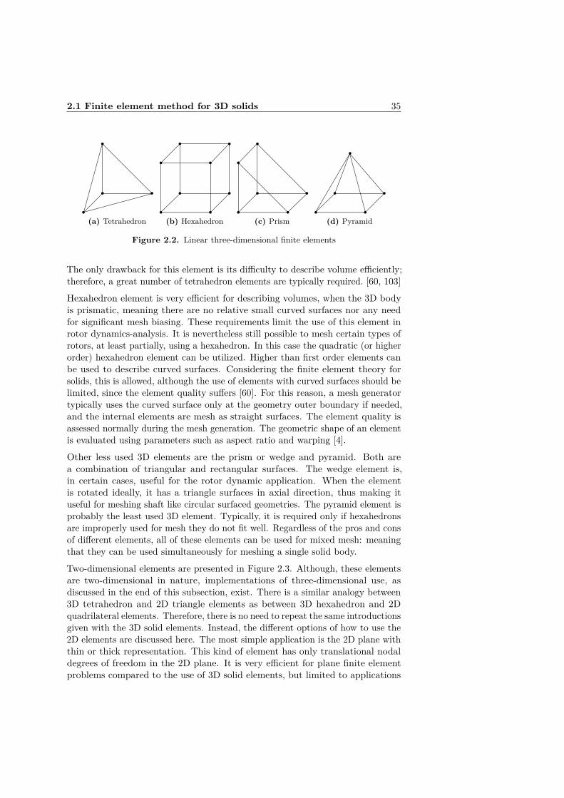
(a) Tetrahedron (b) Hexahedron (c) Prism (d) Pyramid
Figure 2.2. Linear three-dimensional finite elements
The only drawback for this element is its difficulty to describe volume efficiently;therefore, a great number of tetrahedron elements are typically required. [60, 103]
Hexahedron element is very efficient for describing volumes, when the 3D bodyis prismatic, meaning there are no relative small curved surfaces nor any needfor significant mesh biasing. These requirements limit the use of this element inrotor dynamics-analysis. It is nevertheless still possible to mesh certain types ofrotors, at least partially, using a hexahedron. In this case the quadratic (or higherorder) hexahedron element can be utilized. Higher than first order elements canbe used to describe curved surfaces. Considering the finite element theory forsolids, this is allowed, although the use of elements with curved surfaces should belimited, since the element quality suffers [60]. For this reason, a mesh generatortypically uses the curved surface only at the geometry outer boundary if needed,and the internal elements are mesh as straight surfaces. The element quality isassessed normally during the mesh generation. The geometric shape of an elementis evaluated using parameters such as aspect ratio and warping [4].
Other less used 3D elements are the prism or wedge and pyramid. Both area combination of triangular and rectangular surfaces. The wedge element is,in certain cases, useful for the rotor dynamic application. When the elementis rotated ideally, it has a triangle surfaces in axial direction, thus making ituseful for meshing shaft like circular surfaced geometries. The pyramid element isprobably the least used 3D element. Typically, it is required only if hexahedronsare improperly used for mesh they do not fit well. Regardless of the pros and consof different elements, all of these elements can be used for mixed mesh: meaningthat they can be used simultaneously for meshing a single solid body.
Two-dimensional elements are presented in Figure 2.3. Although, these elementsare two-dimensional in nature, implementations of three-dimensional use, asdiscussed in the end of this subsection, exist. There is a similar analogy between3D tetrahedron and 2D triangle elements as between 3D hexahedron and 2Dquadrilateral elements. Therefore, there is no need to repeat the same introductionsgiven with the 3D solid elements. Instead, the different options of how to use the2D elements are discussed here. The most simple application is the 2D plane withthin or thick representation. This kind of element has only translational nodaldegrees of freedom in the 2D plane. It is very efficient for plane finite elementproblems compared to the use of 3D solid elements, but limited to applications

36 2 Finite element modeling of rotating structures
that have constant thickness, such as plate geometries. A comparison of thenodal degrees of freedom of different elements is provided in Table 2.1, where urepresents translational degree of freedom and θ represents rotational degree offreedom.
(a) Triangle (b) Quadrilateral
Figure 2.3. Linear two-dimensional finite elements
Table 2.1. Nodal degrees of freedom of certain elements
Element type Nodal degrees of freedom3D solid ux uy uz2D plane ux uyAxisymmetric solid ur uw or ur uw θ3D shell ux uy uz θx θy θz
Figure 2.4. Applications for 2D elements: on the left, the axisymmetric element, andon the right, the 3D shell element [4]
Axisymmetric solids are one practical application for considering rotor dynamicspurposes. The axisymmetric model is very efficient compared to the 3D representa-tion of rotor geometry. The downside of the axisymmetric element is its deficiencywith respect to the description of any complex shapes. The axisymmetric and 3Dshell elements are illustrated in Figure 2.4.
As seen in Figure 2.4, the 3D shell elements can describe 3D surfaces. 3D shellelements may not be useful for modeling rotor components themselves, perhaps,for some features such as turbine blades. But they can be very useful for modelingthe frame of the rotating machine. In comparison, 3D elements typically requires

2.1 Finite element method for 3D solids 37
at least two element layers, even with quadratic elements, in order to to accuratelymodel 3D walls.There are even more uses for a 2D element when the structure is modeled using 3Dsolids. Surface loads such as structural pressure load and convective or radiatingheat transfer loads require integration over the loading surface; thus, 2D elementsare used for surface loads. Also, certain FE-software use 3D shells for contactdetection in the 3D domain. Common isoparametric 2D and 3D elements areintroduced in Appendix B. The shape functions formulated for these isoparametricelements as introduced are given in Appendix A and numerical integration schemesfor isoparametric elements are given in Appendix C.
2.1.2 Energy principle for formulating element matrices
Finite element matrices can be formulated using the energy principle, anddividing it further into kinetic and elastic strain energies. Hamilton’s principleis introduced in references such as Liu and Quek [60], and Lagrangian principlein Kirchgäßner [48]. The outcome of full formulation is the equations of motion.The basic formulations required for mass, gyroscopic and stiffness matrices andfundamental force vectors are presented here.The kinetic energy of translational motion and kinetic energy, due to the gyroscopiceffect can be written as follows [60, 35]:
Tk = Tm + Tg (2.3)
where Tm is the kinetic energy of translational motion and TG is the kinetic energydue to the gyroscopic effect. Based on Tm and TG expressions, element mass andgyroscopic damping matrices can be formulated, respectively. The kinetic energyof translational motion can be written as follows:
Tm = 12
∫VρuTudV (2.4)
where ρ is the material density. Three-dimensional displacement interpolationusing shape functions can be written as follows [103]:
u = Nde =n∑i=1
Nidi (2.5)
The element displacement vector can be written as follows [60]:
u =
uvw
(2.6)
The nodal displacement vector can be written as follows:
38 2 Finite element modeling of rotating structures
di =
uiviwi
(2.7)
When substituting Equation (2.5) in Equation (2.4), the kinetic energy of transla-tional motion can be written as follows:
Tm = 12 d
Te
(∫VρNTNdV
)de (2.8)
Based on Equation (2.8), symmetric element mass matrix can be written asfollows:
Me =∫VρNTNdV (2.9)
Element shape function matrix N can be written as follows:
N =[N1 N2 · · · Nn
](2.10)
where n is the number of element shape functions. Element shape function matrixof node i Ni can be written as follows:
Ni =
Ni 0 00 Ni 00 0 Ni
(2.11)
where Ni is the ith shape function of an element. Shape functions for common3D solid elements are introduced in Appendix B. Considering the rotation aroundthe global X-axis, general kinetic energy due to the gyroscopic effect, adoptedfrom [35, 101], can be written as follows:
Tg = −∫Vρθxu
(θyy + θzz
)dV (2.12)
where
θx = Ωt (2.13)
θy = 12
(∂u
∂z− ∂w
∂x
)(2.14)
θz = 12
(∂v
∂x− ∂u
∂y
)(2.15)
2.1 Finite element method for 3D solids 39
By substituting Equations (2.13–2.15) into Equation (2.12) and replacing dis-placements with shape functions and generalized coordinates according to Equa-tion (2.5), kinetic energy due to the gyroscopic effect for solid elements can bewritten as follows:
Tg = Ωn∑i=1
n∑j=1
(ui
(12ρ∫V
(∂Ni
∂yNjzi −
∂Ni
∂zNjyi
)dV
)uj
+vi(−1
2ρ∫V
∂Ni
∂xNjzidV
)uj + wi
(12ρ∫V
∂Ni
∂xNjyidV
)uj
) (2.16)
Equation (2.16) can be written in matrix form, as follows:
Tg = Ωn∑i=1
d
Te,i
12ρ∫V
∂Ni
∂yzi −
∂Ni
∂zyi 0 0
−∂Ni
∂xzi 0 0
∂Ni
∂xyi 0 0
NdV
de = ΩdT
e Gede (2.17)
Based on Equation (2.17), the skew-symmetric element gyroscopic damping matrixcan be written as follows [101]:
Ge = Ge −GeT (2.18)
Based on the strain energy expression, the element elastic stiffness matrix can beformulated. The strain energy can be written as follows [60]:
Π = 12
∫VεTσdV (2.19)
The element strain vector can be written as follows:
ε = Lu (2.20)
Strain-displacement relationships for linear isotropic material in 3D domain canbe written as follows [61]:

40 2 Finite element modeling of rotating structures
εx = ∂u
∂x
εy = ∂v
∂y
εz = ∂w
∂z
γxy = ∂u
∂y+ ∂v
∂x= γyx
γyz = ∂v
∂z+ ∂w
∂y= γzy
γzx = ∂w
∂x+ ∂u
∂z= γxz
(2.21)
The matrix of partial differential operations can be written as follows [61]:
L =
∂/∂x 0 00 ∂/∂y 00 0 ∂/∂z
∂/∂y ∂/∂x 00 ∂/∂z ∂/∂y
∂/∂z 0 ∂/∂x
(2.22)
The element stress vector can be written as follows:
σ = Dε (2.23)
The matrix of material constants D for linear isotropic material is expressed as
D = E
(1 + ν) (1− 2ν)
1− ν ν ν 0 0 0ν 1− ν ν 0 0 0ν ν 1− ν 0 0 00 0 0 1−2ν
2 0 00 0 0 0 1−2ν
2 00 0 0 0 0 1−2ν
2
(2.24)
where E is the elastic modulus and ν is the Poisson’s ratio [61]. The elementstrain matrix B can be written as follows:
B = LN (2.25)
By substituting Equations (2.20), (2.23) and (2.25) in Equation (2.19), the strainenergy can be written as follows:
Π = 12d
Te
(∫V
BTDBdV)de (2.26)

2.1 Finite element method for 3D solids 41
Symmetric element elastic stiffness matrix can be written as follows
Kee =
∫V
BTDBdV (2.27)
Elastic damping matrix using proportional damping expression based on stiffnessand mass matrices can be written as follows [3]:
Ce = αpKe + βpM (2.28)
where αp and βp are proportional coefficients for stiffness and mass matrices.
Formulation of external force vectors
Element body and surface force vectors can be formulated from virtual workprinciple. Work done by external forces can be written as follows [60]:
Wf =∫VuTf ebdV +
∫SuTf esdS (2.29)
By substituting Equation (2.5) into Equation (2.29) the work done by externalforce can be written as follows:
Wf = dTe
(∫V
NTf ebdV
)+ dT
e
(∫S
NTf esdS
)(2.30)
The element nodal body force vector can be written as follows:
f eb =
fxfyfz
(2.31)
The element nodal surface force vector can be written as follows:
f es =
fxfyfz
(2.32)
The nodal surface force vector is having same analogy than in Equation (2.31).Element body force vector can be written as follows:
F eb =
∫V
NTf ebdV (2.33)
Element surface force vector can be written as follows:

42 2 Finite element modeling of rotating structures
F es =
∫S
NTf esdS (2.34)
Total work done by external force is thus given as
Wf = dTe F
eb + dT
e Fes = dT
e Feext (2.35)
where F eext is the element total external force vector.
Stress-stiffening effect
The stress stiffness matrix can be used for eigenvalue analysis of the pre-stressedstructure. Stress stiffening – also known as geometric stiffening – for a singleelement can be written as follows [48]:
KeG =
∫V
BTε S0BεdV (2.36)
The matrix Bε containing the spatial derivatives of the element shape functionscan be written as follows:
Bε =
I3∂N1∂x
I3∂N2∂x
· · · I3∂Nn
∂x
I3∂N1∂y
I3∂N2∂y
· · · I3∂Nn
∂y
I3∂N1∂z
I3∂N2∂z
· · · I3∂Nn
∂z
(2.37)
and the initial stress matrix S0 is
S0 =
I3σx I3τxy I3τxzI3τyx I3σy I3τyzI3τzx I3τzy I3σz
(2.38)
where I3 is a 3 × 3 identity matrix. The element stress vector can be written asfollows [61]
σx σy σz τxy τyz τzxT = DBu (2.39)
where σx σy σz are the element normal stress components and τxy τyz τzxare the element shear stress components. Element-based normal stress and shearstress components are illustrated in Figure 2.5. Note that for linear isotropicmaterial, the strain components are equal in the following manner

2.1 Finite element method for 3D solids 43
τxy = τyx
τyz = τzy
τzx = τxz
(2.40)
Y
Z
X
τzy
σz
τzx
σy
τyz
τyx
τxy
τxz
σx
τzy
σz
τzx
τxy
τxz
σx
σy
τyz
τyx
Figure 2.5. Three-dimensional stress components
Common force vectors for structural analysis
Formulations of 3D solid element force vectors for centrifugal force, translationalacceleration, surface pressure and thermal expansion are presented. The elementcentrifugal force vector can be written as follows [48]:
Ω2F eΩ = Ω2
n∑i=1
ρ
∫V
NTi ΩTΩxidV (2.41)
where xi is the vector of coordinates of node i. The matrix Ω indicating the axisof rotation can be written as follows:
Ω =
0 −ωz ωyωz 0 −ωx−ωy ωx 0
(2.42)

44 2 Finite element modeling of rotating structures
where ωx, ωy and ωz are the normalized angular velocity components, accordingto the global coordinate system, |ωx ωy ωz| = 1. Based on Newton’s secondlaw, the general element translational acceleration force vector can be written asfollows:
F eg = ρ
∫V
NTgadV (2.43)
where
ga =
gxgygz
(2.44)
where gx, gy and gz are the translational acceleration components, according tothe Cartesian coordinate system. By applying the standard acceleration of gravityinto Equation (2.44), the gravitational body force can be modeled. Elementpressure force vector can be written as follows:
F ep =
∫S
NTppdS (2.45)
where
pp =
pxpypz
(2.46)
where px, py and pz are the pressure normal component according to the Cartesiancoordinate system. The element force vector due to initial strain can be writtenas follows [103]:
F eε =
∫V
BTDε0dV (2.47)
where
ε0 =
εx,0εy,0εz,0γxy,0γyz,0γzx,0
(2.48)
The linear thermal expansion can be written as follows:
∆L = Lα (T − Tref) (2.49)

2.1 Finite element method for 3D solids 45
Thus, strain ε can be written as follows:
ε = ∆LL
= α∆T (2.50)
where α is the thermal expansion coefficient. The nodal temperature can benon-uniform over the element. Thus, by expanding the Equation (2.50) intothree-dimensional domain and substituting it into Equation (2.47), the elementthermal expansion force vector can be written as follows [28]:
F e∆T =
n∑i=1
∫V
BTi Dα∆TidV (2.51)
where ∆Ti is the temperature difference of node i. The vector α can be writtenas follows:
α =
αxαyαz000
(2.52)
2.1.3 Heat transfer theory
The heat transfer equation is introduced in this subsection. Heat transfer analysiscan be coupled with structural analysis if a structure is experiencing thermal loadssuch as internal heat generation or boundary heat flow from solid into medium. Inthis case, the need for solving the thermal state of a structure becomes necessaryfor analyzing the effect of thermal expansion-induced stresses. The heat transferequation can be written as follows [76]:
−(∂qx∂x
+ ∂qy∂y
+ ∂qz∂z
)+Q = ρc
∂T
∂t(2.53)
where qx, qy and qz are the components of heat flow through the unit area, Q isthe internal heat generation rate per unit volume, ρ is the material density, c isthe specific heat capacity, T is the temperature and t is the time. The heat flowcomponents in isotropic case can be written as follows:
qx = −kx∂T
∂x
qy = −ky∂T
∂y
qz = −kz∂T
∂z
(2.54)

46 2 Finite element modeling of rotating structures
where kx, ky and kz are the thermal conductivity coefficients in global X, Yand Z-directions, respectively. By substituting the heat flow components inEquation (2.53), the heat transfer equation can be written as follows:
∂
∂x
(kx∂T
∂x
)+ ∂
∂y
(ky∂T
∂y
)+ ∂
∂z
(kz∂T
∂z
)+Q = ρc
∂T
∂t(2.55)
There are four typical loading types to be used with the heat equation: theinternal volumetric heat generation, boundary surface heat flow according toEquation (2.56), boundary surface convection heat transfer according to Equa-tion (2.57), and heat radiation, which is excluded from the heat equation. Inaddition, a fixed temperature on surface or on a single node can be used as theboundary condition.
qxnx + qyny + qznz = −qs (2.56)
qxnx + qyny + qznz = h (Ts − Te) (2.57)
where h is the convection coefficient, Ts is the surface temperature and Te is thereference temperature for convective heat transfer. This reference temperatureis normally the ambient temperature of the fluid on the boundary surface of astructural domain.
2.1.4 Finite element method for three-dimensional heat transfer
In this subsection, thermal modeling using the 3D solid finite element methodis introduced. Formulation of heat transfer matrices and loading vectors aregiven. Using the Galerkin method, the heat transfer equation can be written asfollows [76]:
∫V
(∂qx∂x
+ ∂qy∂y
+ ∂qz∂z−Q+ ρc
∂T
∂t
)NidV = 0 (2.58)
∫Vρc∂T
∂tNidV −
∫V
[∂Ni
∂x
∂Ni
∂y
∂Ni
∂z
]qdV
=∫VQNidV −
∫SqTnNidS
+∫SqsNidS −
∫Sh (Ts − Te)NidS
(2.59)
where
qT = [qx qy qz]nT = [nx ny nz]
(2.60)
2.1 Finite element method for 3D solids 47
where n is an outer normal to the surface of the body. The finite element equationfor heat transfer can be written as follows:
CTN + (KC + Kh)TN = RT +RQ +Rq +Rh (2.61)
whereC is the heat capacity matrixKC is the heat conduction matrixKh is the surface convection matrixTN is the nodal temperature vectorRT is the specified boundary temperature vectorRQ is the internal heat generation vectorRq is the boundary heat flow vectorRh is the surface convection vector
The element heat capacity matrix can be written as follows:
Ce =∫VρcNTNdV (2.62)
where the vector of element shape functions N can be written as follows [24]:
N =[N1 N2 · · · Nn
](2.63)
The element heat conduction matrix can be written as follows [76]:
KeC =
∫V
BTd DcBddV (2.64)
where Bd is the matrix of shape function derivatives and Dc the conductivitymatrix. The matrix of shape function derivatives can be written as follows:
Bd =
∂/∂x∂/∂y∂/∂z
N (2.65)
The conductivity matrix can be written as follows [24]:
Dc =
kx 0 00 ky 00 0 kz
(2.66)
The element surface convection matrix can be written as follows:
Keh =
∫ShNTNdS (2.67)
48 2 Finite element modeling of rotating structures
The element specified boundary temperature vector can be written as follows:
ReT = −
∫SqTnNTdS (2.68)
The element internal heat generation vector can be written as follows:
ReQ =
∫VQNTdV (2.69)
The element boundary heat flow vector can be written as follows:
Req =
∫SqsN
TdS (2.70)
The element surface convection vector can be written as follows:
Reh =
∫ShTeN
TdS (2.71)
2.2 Constraint equations and contact modeling
In this subsection, the concept constraint equation is introduced, and multipledifferent methods of applying constrain equations are presented. Constraintequation is an equation which describes the motion between two or more degreesof freedom. Boundary condition, such as a DOF displacement, can be defined byapplying the constraint equation to a boundary DOF in the model. In such acase, the constraint equation is applied between a particular boundary DOF andthe ground; thus, it is referred to as boundary constraint. Similarly, boundaryconstraints such as cyclic symmetry can be described. Four different constraintmodeling methods are introduced: master-slave, penalty function, Lagrangianmultiplier method [29, 102, 103, 104], and a novel proposed application specificconstraint method called trial force method developed in [91]. Constraint equationsare implemented inside the stiffness matrix, and they limit the movement ofunconstrained DOFs. Two main types of constraint equations are considered: ho-mogeneous equations that constraints the DOF movement, and non-homogeneousequations that describe how a single DOF can move in accordance with oneor more DOFs. In Figure 2.6, the procedure of using constraint equations ispresented.
Master-slave and penalty function methods both use direct stiffness matrixmanipulation, which yields the desired displacement vector output, but notthe force vector corresponding to the constrained structure. Direct manipulationin this instance considers the manipulation of stiffness terms to be directly relatedto the DOFs of a particular constraint equation. Both the Lagrangian multiplierand trial force method do not use direct stiffness matrix manipulation, whichyields the desired displacement vector output and the force vector corresponding
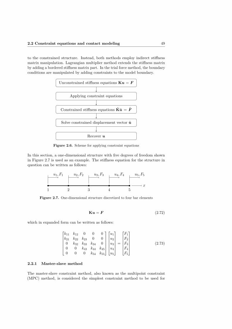
2.2 Constraint equations and contact modeling 49
to the constrained structure. Instead, both methods employ indirect stiffnessmatrix manipulation. Lagrangian multiplier method extends the stiffness matrixby adding a bordered stiffness matrix part. In the trial force method, the boundaryconditions are manipulated by adding constraints to the model boundary.
Unconstrained stiffness equations Ku = F
Applying constraint equations
Constrained stiffness equations Ku = F
Solve constrained displacement vector u
Recover u
Figure 2.6. Scheme for applying constraint equations
In this section, a one-dimensional structure with five degrees of freedom shownin Figure 2.7 is used as an example. The stiffness equation for the structure inquestion can be written as follows:
x1
u1, F1
2
u2, F2
3
u3, F3
4
u4, F4
5
u5, F5
Figure 2.7. One-dimensional structure discretized to four bar elements
Ku = F (2.72)
which in expanded form can be written as follows:
k11 k12 0 0 0k21 k22 k23 0 00 k32 k33 k34 00 0 k43 k44 k450 0 0 k54 k55
u1u2u3u4u5
=
F1F2F3F4F5
(2.73)
2.2.1 Master-slave method
The master-slave constraint method, also known as the multipoint constraint(MPC) method, is considered the simplest constraint method to be used for

50 2 Finite element modeling of rotating structures
presenting the use of the homogeneous constraint equation. [29] Let us apply aconstraint to the structure given in Figure 2.7 between DOFs u2 and u4 as follows:
u2 = u4 (2.74)
Based on Equation (2.74), let us propose that DOF u4 is a slave of DOF u2,thus u4 has to move exactly the same quantity than DOF u2. Let us introduce atransformation matrix T to apply the constraint equation given in Equation (2.74)as follows:
u1u2u3u4u5
=
1 0 0 00 1 0 00 0 1 00 1 0 00 0 0 1
u1u2u3u5
(2.75)
where the transformation matrix T is originally a square identity matrix size ofn× n, where n is the number of DOFs. In the transformation matrix T, the rowof the slave DOF is replaced with the row of the master DOF, and the column ofthe slave DOF is removed. Using matrix notation, the described transformationsof matrix T can be written as follows:
T = In×nT k = T i
T j = ∅, i = j
(2.76)
where subscripts n, i, k and j are the number of DOFs, ith row correspondingto the master DOF, kth row corresponding to the slave DOF and jth columncorresponding to the master DOF, respectively, and ∅ is the symbol for the emptyset representing an empty column vector. This method can be impractical forhandling multiple constraints. Thus, an alternative method for manipulating thetransformation matrix T and introduction of diagonal matrix Td can be writtenas follows:
T = In×nT k = T i
Td = 0n×nTd,ij = 1, i = j
(2.77)
where subscripts n, i and k are the number of DOFs, ith row correspondingto the master DOF and kth row corresponding to the slave DOF and Td
is the transformation matrix containing diagonal terms. This method keepsthe original DOF order and thus is practical to be used for a problem havingmultiple constraints. Although, some numerical solvers of software such as Matlabmay lack the capability to skipping empty rows and column, and thus requires

2.2 Constraint equations and contact modeling 51
additional diagonal markings, therefore the diagonal matrix Td according toEquation (2.77) is required. In Equation (2.80), the use of the Td matrix isintroduced. Equation (2.75) can be written as follows:
u = Tu (2.78)
By replacing Equation (2.75) into (2.72) and multiplying by TT yields modifiedstiffness equations as follows:
Ku = F (2.79)
When using the alternative method for generating the transformation matrix asgiven in Equation (2.77), the modified stiffness matrix can be written as follows:
K = TTKT + Td (2.80)
F = TTF (2.81)
By expanding Equation (2.79), the result can be written as follows:
k11 k12 0 0k21 k22 + k44 k23 + k43 k450 k32 + k34 k33 00 k45 0 k55
u1u2u3u5
=
F1
F2 + F4F3F5
(2.82)
Recovering the slave DOFs can be performed by using Equation (2.78). A set ofmultiple homogeneous constraint equations can be applied. Let us introduce asecond constraint equation as follows:
u1 + 2u3 = 0 (2.83)
Again, selecting the slave DOF, now u3, Equation (2.83) can be written as follows:
u3 = −12u1 (2.84)
When applying both constraint equations (2.74) and (2.83), Equation (2.78) canbe rewritten as follows:
u1u2u3u4u5
=
1 0 00 1 0−1
2 0 00 1 00 0 1
u1u2u5
(2.85)
52 2 Finite element modeling of rotating structures
In addition to homogeneous constraint equations, there are also non-homogeneousconstraint equations that yield differentiating relationship between the constraintDOFs. An example of a non-homogeneous constraint equation can be written asfollows:
u2 − u4 = 2 (2.86)
Again, DOF u4 is selected as slave DOF. Non-homogeneous constraint equationscan be used to model a gap or overlapping to the meshed geometry. Now,Equation (2.78) is expanded by adding a vector for non-homogeneous part of theconstraint equations. Equation (2.78) can be written as follows:
u = Tu+ g (2.87)
where g is the vector of non-homogeneous coefficients. Equation (2.87) in expandedform can be written as follows:
u1u2u3u4u5
=
1 0 0 00 1 0 00 0 1 00 1 0 00 0 0 1
u1u2u3u5
+
000−20
(2.88)
By multiplying Equation (2.87) by TTK and substituting Equation (2.72) intoEquation (2.87) and passing all the terms to the right-hand side, the force vectorcan be written as follows:
F = TT (F + Kg) (2.89)
Equation (2.89) in expanded form can be written as follows:
k11 k12 0 0k21 k22 + k44 k23 + k43 k450 k32 + k34 k33 00 k45 0 k55
u1u2u3u5
=
F1
F2 + F4 − 2k44F3 − 2k34F5 − 2k45
(2.90)
The master-slave constraint method is exact. This method reduces the totalnumber of degrees of freedom, if so desired; it can therefore be regarded as a formof model reduction. Due to the simplicity of the master-slave constraint method,it was used here to introduce homogeneous and non-homogeneous constraintequations. The master-slave method can also be used for kinematic modelreduction, when the displacements of the slave DOFs can be expressed usingseries kinematic constraint equations, though this is rarely useful. In otherwords, the method can be used only if the elastic behavior can be expressed fullykinematically: meaning the structures must be very simple.

2.2 Constraint equations and contact modeling 53
2.2.2 Penalty function method
The penalty function constraint method is easier to implement than the master-slave method. This method uses a fictional, massless, penalty element. [29] Thiselement is elastic, though very stiff, which leads to a situation that the constraintequation using the penalty method is not exact, unlike the master-slave method,owing to the elastic nature of the penalty element. The same structure introducedin Section 2.2 with a penalty element in accordance with constraint equation(2.74) is illustrated in Figure 2.8.
Penalty element
x1
u1, F1
2
u2, F2
3
u3, F3
4
u4, F4
5
u5, F5
Figure 2.8. Five-DOF bar element model with penalty element
The local penalty element stiffness equation can be written as follows:
W
[1 −1−1 1
] [u1u4
]=[00
](2.91)
where W is the penalty weight or the stiffness coefficient for the penalty ele-ment. The penalty method uses full matrices, substituting Equation (2.91) inEquation (2.73) using global DOFs yields
k11 k12 0 0 0k21 k22 +W k23 −W 00 k32 k33 k34 00 −W k43 k44 +W k450 0 0 k54 k55
u1u2u3u4u5
=
F1F2F3F4F5
(2.92)
Multiple DOF constraint equations can be applied using the penalty method. Letus consider a non-homogeneous constraint equation as follows:
u1 + 3u4 − 4u5 = 1 (2.93)
Equation (2.93) expressed in matrix form can be written as follows:
[1 3 − 4]
u1u4u5
= 1 (2.94)

54 2 Finite element modeling of rotating structures
By multiplying both sides using the coefficient vector and the penalty weight,Equation (2.94) can be written as follows:
W
1 3 −43 9 −12−4 −12 16
u1u4u5
= W
13−4
(2.95)
By substituting Equation (2.95) in (2.73) using global DOFs, we get
k11 +W k12 0 3W −4Wk21 k22 k23 0 00 k32 k33 k34 0
3W 0 k43 k44 + 9W k45 − 12W−4W 0 0 k54 − 12W k55 + 16W
u1u2u3u4u5
=
F1 +WF2F3
F4 + 3WF5 − 4W
(2.96)
Attention must be paid when selecting the penalty weight. Since the penaltyconstraint using penalty element is not exact, owing to the fact that the penaltyelement has finite stiffness, the penalty weight selected should be as large aspossible. If the penalty coefficient selected is too large, the stiffness matrix maybecome ill-conditioned with respect to inversion.
The constraint error of the penalty method, taking the example non-homogeneousconstraint equation (2.93) into consideration, is eg =| u1 + 3u4 − 4u5 − 1 |. Themagnitude of this constraint error eg is dependent on the penalty weight used.With sufficiently large penalty weights the constraint error becomes 1/W .
The square root rule is provided as a general guide for selecting the penalty weightcoefficient. The rules states that the penalty weight should be W ≈ 10kmax
√10pw ,
where kmax is the magnitude of the largest stiffness coefficient in the unconstrainedstiffness matrix, and pw is the working precision of the software used. [29]
2.2.3 Lagrangian multiplier method
Unlike the penalty function method, the Lagrangian multiplier constraint methodcan be exact. This method uses additional coefficients, Lagrangian multipliersλ, thus increasing the size of global matrices. [29] Let us consider a constraintequation as follows:
u2 = u4 (2.97)
The Lagrangian multiplier constraint, Equation (2.97), can be illustrated as shownin Figure 2.9, where −λ, λ are the constraint forces.
By applying Equation (2.97) the stiffness equation (2.73) we get
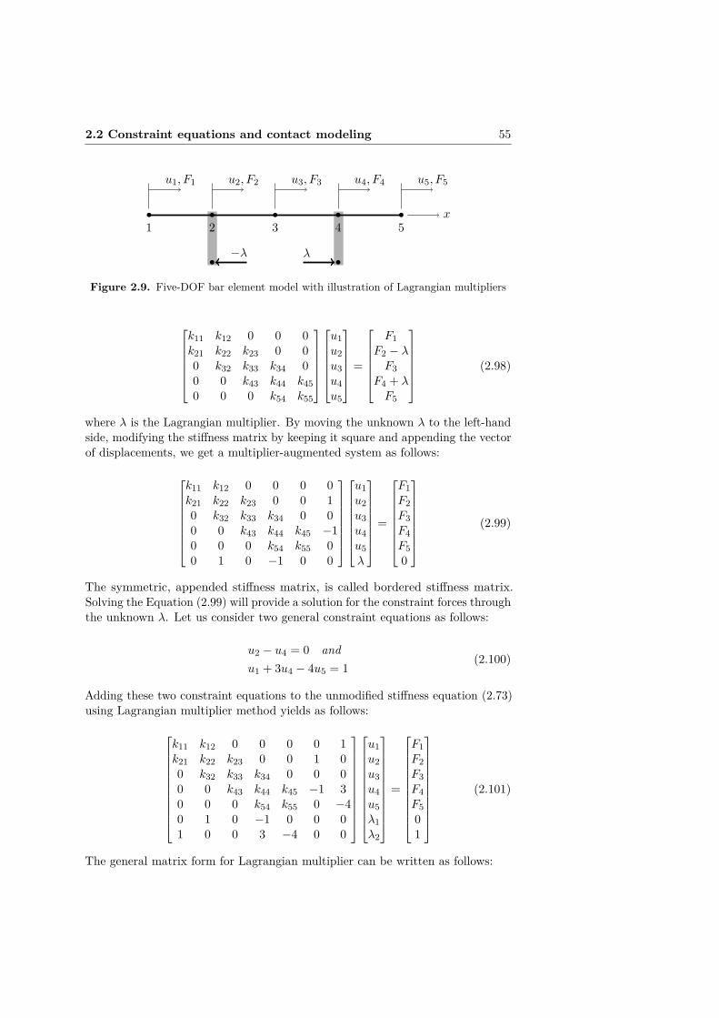
2.2 Constraint equations and contact modeling 55
−λ λ
x1
u1, F1
2
u2, F2
3
u3, F3
4
u4, F4
5
u5, F5
Figure 2.9. Five-DOF bar element model with illustration of Lagrangian multipliers
k11 k12 0 0 0k21 k22 k23 0 00 k32 k33 k34 00 0 k43 k44 k450 0 0 k54 k55
u1u2u3u4u5
=
F1
F2 − λF3
F4 + λF5
(2.98)
where λ is the Lagrangian multiplier. By moving the unknown λ to the left-handside, modifying the stiffness matrix by keeping it square and appending the vectorof displacements, we get a multiplier-augmented system as follows:
k11 k12 0 0 0 0k21 k22 k23 0 0 10 k32 k33 k34 0 00 0 k43 k44 k45 −10 0 0 k54 k55 00 1 0 −1 0 0
u1u2u3u4u5λ
=
F1F2F3F4F50
(2.99)
The symmetric, appended stiffness matrix, is called bordered stiffness matrix.Solving the Equation (2.99) will provide a solution for the constraint forces throughthe unknown λ. Let us consider two general constraint equations as follows:
u2 − u4 = 0 andu1 + 3u4 − 4u5 = 1
(2.100)
Adding these two constraint equations to the unmodified stiffness equation (2.73)using Lagrangian multiplier method yields as follows:
k11 k12 0 0 0 0 1k21 k22 k23 0 0 1 00 k32 k33 k34 0 0 00 0 k43 k44 k45 −1 30 0 0 k54 k55 0 −40 1 0 −1 0 0 01 0 0 3 −4 0 0
u1u2u3u4u5λ1λ2
=
F1F2F3F4F501
(2.101)
The general matrix form for Lagrangian multiplier can be written as follows:
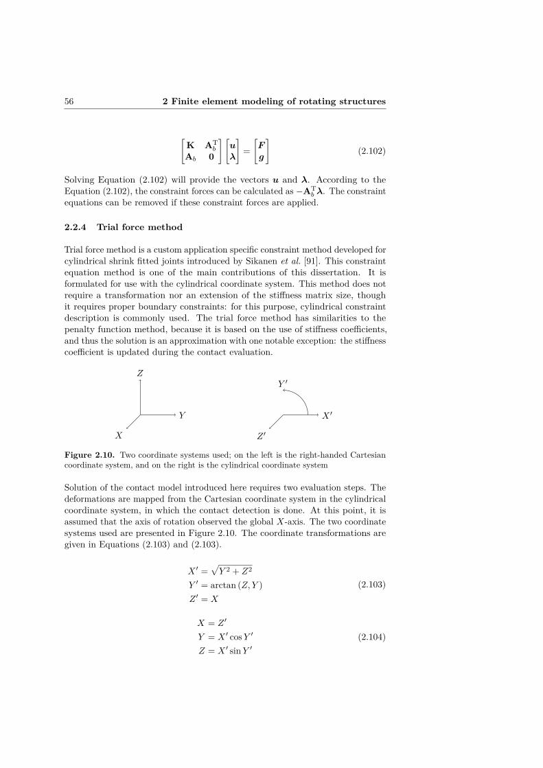
56 2 Finite element modeling of rotating structures
[K AT
b
Ab 0
] [uλ
]=[Fg
](2.102)
Solving Equation (2.102) will provide the vectors u and λ. According to theEquation (2.102), the constraint forces can be calculated as −AT
b λ. The constraintequations can be removed if these constraint forces are applied.
2.2.4 Trial force method
Trial force method is a custom application specific constraint method developed forcylindrical shrink fitted joints introduced by Sikanen et al. [91]. This constraintequation method is one of the main contributions of this dissertation. It isformulated for use with the cylindrical coordinate system. This method does notrequire a transformation nor an extension of the stiffness matrix size, thoughit requires proper boundary constraints: for this purpose, cylindrical constraintdescription is commonly used. The trial force method has similarities to thepenalty function method, because it is based on the use of stiffness coefficients,and thus the solution is an approximation with one notable exception: the stiffnesscoefficient is updated during the contact evaluation.
Y
Z
X
X ′
Z ′
Y ′
Figure 2.10. Two coordinate systems used; on the left is the right-handed Cartesiancoordinate system, and on the right is the cylindrical coordinate system
Solution of the contact model introduced here requires two evaluation steps. Thedeformations are mapped from the Cartesian coordinate system in the cylindricalcoordinate system, in which the contact detection is done. At this point, it isassumed that the axis of rotation observed the global X-axis. The two coordinatesystems used are presented in Figure 2.10. The coordinate transformations aregiven in Equations (2.103) and (2.103).
X ′ =√Y 2 + Z2
Y ′ = arctan (Z, Y )Z ′ = X
(2.103)
X = Z ′
Y = X ′ cosY ′
Z = X ′ sinY ′(2.104)
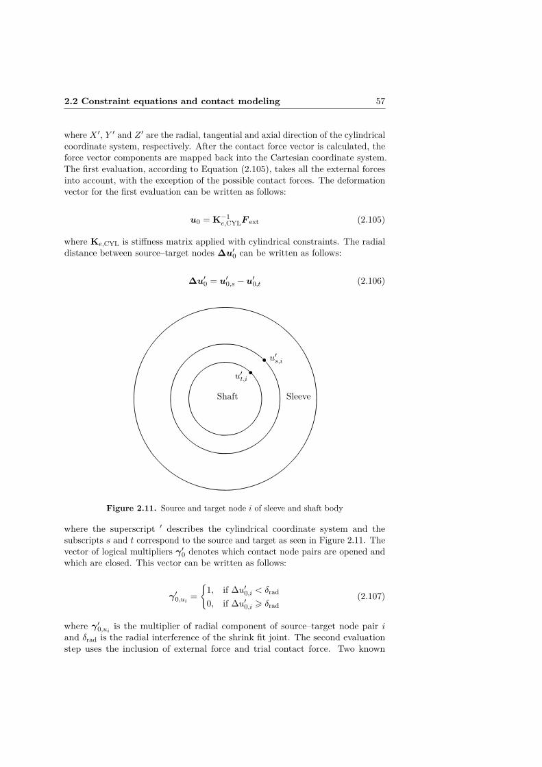
2.2 Constraint equations and contact modeling 57
where X ′, Y ′ and Z ′ are the radial, tangential and axial direction of the cylindricalcoordinate system, respectively. After the contact force vector is calculated, theforce vector components are mapped back into the Cartesian coordinate system.The first evaluation, according to Equation (2.105), takes all the external forcesinto account, with the exception of the possible contact forces. The deformationvector for the first evaluation can be written as follows:
u0 = K−1e,CYLF ext (2.105)
where Ke,CYL is stiffness matrix applied with cylindrical constraints. The radialdistance between source–target nodes ∆u′0 can be written as follows:
∆u′0 = u′0,s − u′0,t (2.106)
u′t,i
u′s,i
Shaft Sleeve
Figure 2.11. Source and target node i of sleeve and shaft body
where the superscript ′ describes the cylindrical coordinate system and thesubscripts s and t correspond to the source and target as seen in Figure 2.11. Thevector of logical multipliers γ ′0 denotes which contact node pairs are opened andwhich are closed. This vector can be written as follows:
γ ′0,ui =
1, if ∆u′0,i < δrad
0, if ∆u′0,i > δrad(2.107)
where γ ′0,ui is the multiplier of radial component of source–target node pair iand δrad is the radial interference of the shrink fit joint. The second evaluationstep uses the inclusion of external force and trial contact force. Two known
58 2 Finite element modeling of rotating structures
variables, external force F ext and trial contact force F c,trial, help in determiningthe unknown contact stiffness kfk0. The final contact force F ′c can be calculatedby solving the contact stiffness. The deformation vector in global Cartesiancoordinates for the second evaluation can be written as follows:
utrial = K−1e,CYL (F ext + F c,trial) (2.108)
where F ′c,trial is the vector of trial contact force in the cylindrical coordinatesystem written as follows:
F ′c,trial = k0∆u′0 · γ ′0 (2.109)
where k0 is the initial value for the contact stiffness. The final contact force vectorcan be written as follows:
F ′c = kf · F ′c,trial (2.110)
where kf is the vector of multipliers for initial contact stiffness. When using thelinear isotropic material model, the multiplier for source–target node pair i isgiven as follows:
δrad −∆u′0,i − kf,i(∆u′trial,i −∆u′0,i
)γ′0,ui = 0 (2.111)
If γ′0,ui = 1, then
kf,i =δrad −∆u′0,i
∆u′trial,i −∆u′0,i(2.112)
The vector ∆u′trial calculated as based on the trial evaluation can be written asfollows:
∆u′trial = u′trial,s − u′trial,t (2.113)
Since the trial force method does not use cross coupling stiffness terms in thestiffness matrix, the solution of stiffness equations can be distributed as expressedin Equation (2.114) by rearranging the equations:
Kassemblyutot = F tot[Kshaft 0
0 Ksleeve
] [ushaftusleeve
]=[F tot,shaftF tot,sleeve
](2.114)
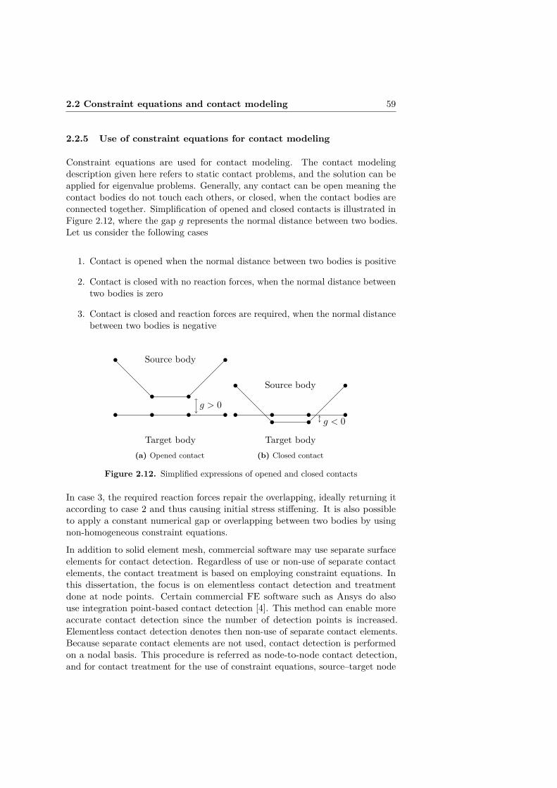
2.2 Constraint equations and contact modeling 59
2.2.5 Use of constraint equations for contact modeling
Constraint equations are used for contact modeling. The contact modelingdescription given here refers to static contact problems, and the solution can beapplied for eigenvalue problems. Generally, any contact can be open meaning thecontact bodies do not touch each others, or closed, when the contact bodies areconnected together. Simplification of opened and closed contacts is illustrated inFigure 2.12, where the gap g represents the normal distance between two bodies.Let us consider the following cases
1. Contact is opened when the normal distance between two bodies is positive
2. Contact is closed with no reaction forces, when the normal distance betweentwo bodies is zero
3. Contact is closed and reaction forces are required, when the normal distancebetween two bodies is negative
Source body
Target body
g > 0
(a) Opened contact
Source body
Target body
g < 0
(b) Closed contact
Figure 2.12. Simplified expressions of opened and closed contacts
In case 3, the required reaction forces repair the overlapping, ideally returning itaccording to case 2 and thus causing initial stress stiffening. It is also possibleto apply a constant numerical gap or overlapping between two bodies by usingnon-homogeneous constraint equations.
In addition to solid element mesh, commercial software may use separate surfaceelements for contact detection. Regardless of use or non-use of separate contactelements, the contact treatment is based on employing constraint equations. Inthis dissertation, the focus is on elementless contact detection and treatmentdone at node points. Certain commercial FE software such as Ansys do alsouse integration point-based contact detection [4]. This method can enable moreaccurate contact detection since the number of detection points is increased.Elementless contact detection denotes then non-use of separate contact elements.Because separate contact elements are not used, contact detection is performedon a nodal basis. This procedure is referred as node-to-node contact detection,and for contact treatment for the use of constraint equations, source–target node

60 2 Finite element modeling of rotating structures
Source body
Target body
Node-to-node source–target node pairs
us,1
us,2 us,3
us,4
ut,1 ut,2 ut,3 ut,4
∆u1
∆u2 ∆u3
∆u4
Figure 2.13. Illustration of elementless node-to-node contact detection
pairs are formed. A simplified illustration of node-to-node contact detection andsource–target node pairs between two bodies is provided in Figure 2.13.
Here, the contact details specified to rotor dynamics use are discussed. Let usconsider a shrink fitted shaft–sleeve contact. The starting point would be a cleanunmodified geometry, and the contact specific geometric modification would bedone only as numerical modifications.
• If external forces are not present, the normal distance between two bodiesmust be increased to the required radial shrink fit value by applying non-homogeneous constraints.
• If external forces are present but the normal distance between two bodiesremains smaller than the required radial shrink fit value, non-homogeneousconstraints must be applied to increase the normal distance to the requiredradial shrink fit value.
• If external forces are present and the normal distance between two bodiesis greater than the required radial shrink fit value, no contact treatment isrequired.
Certain meshing tools can create a mesh where nodes of the source and targetsurface are overlapping, meaning the distance between source and target nodes iszero, thus enabling node-to-node contact. If the overlapping node discretizationon the contact region of two different bodies is not achieved by the mesh generator,other methods may be used. One method is node duplication; the contact regionbetween two bodies must be removed by combining these bodies into a group,and after meshing the duplication of nodes on this boundary must be done.Another method is to form node groups and interpolate weight coefficients forthese grouped nodes; in terms of contact force vectors, one source node is selectedand, for example, the three closest corresponding target nodes are selected andthe contact reaction force is divided for these target nodes using proper weightcoefficients. The latter method given here is not used in this dissertation.

2.2 Constraint equations and contact modeling 61
2.2.6 Summary on constraint equations
The master-slave method is exact, but because of the forced displacements used,the global force vector should be evaluated and inspected for the possible presenceof extremely high amplitude force components. If this method is improperly usedfor structural stress analysis, extreme hot spot stress peaks may appear in nearproximity of the constrained surface. The analyst must pay attention to theseevaluated forces and, if needed, use a different constraint method. Also, the useof the transformation matrix with sparse matrices may cause unwanted excessiveuse of the random-access memory.
The penalty function method is a good choice for the general contact problem,because of the use of the penalty weight. This method is based on the use ofa stiffness coefficient and should reach accurate force equilibrium, though theconvergence of the solution is dependent on the penalty weight used. If too largeweight is used, the stiffness matrix may become ill-conditioned and the solutioninaccurate. The accuracy of this method is proportional to the magnitude penaltyweight used.
Use of the Lagrangian method will extend the stiffness matrix size. Althoughthe bordered matrix added may be sparse enough, the total number unknownsis nevertheless increased. On the other hand, the part in the modified stiffnessmatrix storing the original stiffness equations remains unchanged, thereby differingfrom the master-slave or penalty function method. This method yields an accuratesolution, and the Lagrangian multiplier contains the information about theconstraint forces. Neither, the MPC and Lagrangian method, do not allowresidual penetration in the contact. Because of this, these methods may not wellsuited for transient analysis, because the contact may oscillate between openedand closed status.
The trial force method is a custom application-specific constraint method developedfor the purposes of modeling shrink-fitted joints for rotor dynamics analyses. Forthis reason, the formulation is provided in the cylindrical coordinate system. Thismethod is unique to other constraint methods presented. The trial force methodis used typically with cylindrical constraints applied, and the actual contacttreatment is handled by manipulating the total external force vector.
The augmented Lagrangian method based on the use of Lagrangian multipliersfrom the Lagrangian method and penalty weight from penalty function method.This method is, perhaps, the most complex constraint equation method, but italso has certain benefits. Many commercial FE software support this method.The main reasons would be data storage and the fact that the unconstrainedstiffness matrix may be kept unmodified. In addition, contact convergence ismuch easier due to the augmented part, because minor residual penetration ofthe contact region is allowed. With an exact constraint method, contact canonly be either opened or closed. This can cause unwanted oscillation between
62 2 Finite element modeling of rotating structures
opened and closed contact status, especially during transient structural analysis.Stiffness coefficient based methods introduced, the penalty function, trial forceand augmented Lagrangian methods, may be used in transient analysis withproper contact damping. These method allow residual penetration in the contact,thus no oscillation of contact status should appear.
Different constraint methods have varying requirements for solving the stiffnessequations. When using Lagrangian based method, the system of linear equationsmust be solved directly, which can be computationally more expensive [4]. Thepenalty function method and trial force method, on the other hand, do not requiredirect solution: the solution of the system of linear equations can be iterative, thuscomputationally more effective. This is typically achieved using an iterative solverobtaining a solution in the system of linear equations [4]. The use of an iterativesolver may, however, results in a minor error in the solution, since the solution isobtained when the tolerance, or error margin, is passed. The trial force methoddoes have another beneficial feature. The penalty function method uses crosscoupling terms in the modified stiffness matrix. The trial force method does notrequire these cross coupling terms: thus, by rearranging the equations, the stiffnessequations can be distributed as expressed in Equation (2.114). By doing so, thesolution for a smaller system of linear equation – for a single body, for example –can be obtained using either a full or iterative solver routine. In addition, if sodesired, various DOF reduction methods such as the static condensation methodcan be implemented, making the problem solution even more computationallyeffective.
2.3 Solution methods
Solution methods for pre-stressed eigenvalue problem with contact non-linearities,for transient thermal mechanical stress analysis and for the transient rotordropdown event simulation, are provided. The theory of undamped and dampedeigenvalue problems is also given. The solution routines are presented in the formof flowcharts. The results presented in Section 3 are produced using the solutionmethods introduced.
2.3.1 Undamped and damped eigenvalue problem
Undamped and damped eigenvalue problems with regard to rotor dynamicsanalysis are presented. The solution routine for generating a Campbell diagramincluding contact non-linearities and the stress-stiffening effect is proposed.
Undamped eigenvalue problem
The undamped eigenvalue problem is used to study structures without any

2.3 Solution methods 63
damping, including gyroscopic damping. The equation of motion can be writtenas follows
Mx+ Ktotx = 0 (2.115)
where Ktot contains all stiffness properties: elastic structural stiffness, possiblebearing stiffness components, possible contact stiffness description and possiblestress-stiffening description. The eigenvalue equation for undamped problem canbe written as follows [60]:
(Ktot − λiM) zi = 0 (2.116)
where zi is the eigenvector and λi is the eigenvalue of the ith eigenmode. Ifmatrices are not symmetrical, the eigenvalue solution yields complex eigenvalues.
Damped eigenvalue problem
The damped eigenvalue problem, also known as the quadratic eigenvalue problem,is used to study the rotating structures for such purposes as generating a Campbelldiagram. The equation of motion can be written as follows:
Mx+ (Ctot + ΩG) x+ Ktotx = 0 (2.117)
The following non-symmetric state space matrix A can be formed from Equa-tion (2.117).
A =[
0 I−M−1Ktot −M−1 (Ctot + ΩG)
](2.118)
where Ktot contains all stiffness properties: elastic structural stiffness, possiblebearing stiffness components, possible contact stiffness description and possiblestress-stiffening description. Similarly, Ctot contains all damping properties:elastic damping, possible bearing damping components and possible contactdamping description. The eigenvectors and eigenvalues are provided by solvingthe eigenvalue problem [38]
Azi = λizi (2.119)
Damped eigenvalues appear in a form of complex conjugate pairs, the ith eigenvaluepair can be written as follows:
λi = λri ± λiiiu (2.120)

64 2 Finite element modeling of rotating structures
where λri and λii are the real and imaginary parts of eigenvalue i, correspondingly,βi is the damped natural frequency of ith eigenmode and iu is the imaginary unitiu =
√−1. Equation (2.120) can be written as follows [38]:
λi = −ξdi ωn,i ± ωd,iiu (2.121)
where ξdi is the damping ratio, ωn,i is the undamped natural frequency and ωd,i isthe damped natural frequency of eigenmode i, correspondingly. The correlationbetween the damped and undamped natural frequency can be written as follows:
ωd,i = ωn,i
√1− ξd2
i (2.122)
Solution method for Campbell diagram
The solution routine for Campbell diagram for a rotor having multiple parts isintroduced in Figure 2.14. First, using the rotational speed Ω of the analysisstep n, the deformations due to external forces are calculated. Based on initialdeformations, proper contact treatment is performed. If contact remains fully orpartially closed, contact force vector is generated. The total deformations due toexternal forces and contact forces are solved. Based on these deformations, thestresses of the structure are calculated and the stress stiffness matrix is formulated.Bearing coefficient matrices Kb and Cb describing the bearing stiffness anddamping, respectively, are introduced. The description of the contact stiffnessmatrix Kc is given after the general solution routine description.
The undamped eigenvalue problem is solved using the total stiffness Ktot and themass matrix M. A subset of n lowest eigenmode vectors is solved and used toform the modal structural matrices. The use of modal matrices is justified duoto the significantly lower memory consumption while solving the eigenvalues ofthe state space matrix. The solution of the damped eigenvalue problem yieldsthe damped complex conjugated pair eigenvalues, and the damped parts of theconjugated pairs, βi, are stored and plotted with the rotational speed vector, inorder to generate the Campbell diagram.
The contact stiffness matrix Kc describes the connections on the contact regionbetween the source and target nodes of the contact bodies. These stiff connectionsare established by applying the penalty elements between the DOFs of source andtarget nodes. As illustrated in Figure 2.14, the vector of logical multipliers γ ′0 isused to determine which source–target node pairs remain closed and are appliedwith the penalty element, and which node pairs are opened and do not requireany attention.

2.3 Solution methods 65
Rotational speed Ωof analysis step n
Calculate externalforces F ext
Contact treatmentInformation of nodalcontact status γ ′0
Generate contactstiffness matrix Kc
Contact forcevector F c
Solution of totaldisplacements utot =K−1e,CYL (F ext + F c)
Generate stressstiffness matrix KG
Solution of undampedeigenvalue problemusing Ktot = Ke +
Kb + Kc + KG
Subset of n lowesteigenmode vectors
Bearing stiffnessmatrix Kb
Generatemodal matrices
Generate statespace matrix usingmodal matrices, and
Ctot = Ce + Cb
Bearing dampingmatrix Cb
Solution of dampedeigenvalue problem
Figure 2.14. Process diagram for generating Campbell diagram for a rotor model withcontacts
2.3.2 Coupled thermal mechanical analysis
The indirectly coupled thermal mechanical analysis routine, which can be appliedto various of applications such as electric motor rotors, is introduced here.Indirectly coupled, also called as weakly coupled, problem is considered more

66 2 Finite element modeling of rotating structures
memory-efficient than the directly coupled problem, because the systems of linearequations for heat transfer and static structural problems are solved sequentially.Directly coupled problem has tendency to use larger system matrices as the twosets of linear equations, in this case, are directly coupled. The finite elementanalysis (FEA) is performed in two steps: first, a transient thermal study iscarried out over the drive cycle to calculate the temperature distribution. Second,the temperature distribution is applied as an initial thermal condition for everysimulation time step along with other mechanical loads. Figure 2.15 presentsa schematic of thermal mechanical simulation steps describing the inputs andoutput.
Rotational speed Torque
Convection Losses
Transientthermal (FEM)
Temperaturedistribution
Mechanical staticstructural (FEM)
Stress history
Figure 2.15. Process diagram for the thermomechanical stress analysis
In the transient thermal FEA, the temperature distribution of the rotatingmachinery is calculated as a function time. In FE model, the electromagneticheat losses, that can be depended on torque and rotation speed, are modeled asvolumetric heat sources in corresponding bodies, such as magnets and laminationstacks. Convective heat transfer boundaries are applied to the model as boundaryconditions describing the effect of air cooling. The convection coefficients used aredependent on the speed differences and are thereby dependent on the rotationalspeed of the rotor.
In the mechanical static structural FEA, the previously solved temperature historyis used as one of the input loads. In every simulation step, the thermal expansioneffect must be converted into expanding body force distribution in order to provide

2.3 Solution methods 67
superposition of all the mechanical forces. The conversion from temperature intoforce is done as a pre-process by first calculating only the strain caused by thermalexpansion, and then the strain state is converted into the body force vector. Afterthis, the rest of the mechanical forces are applied, the tangential forces generatedby the torque, and the centrifugal forces from the rotational speed. Finally, allthe mechanical forces are combined to solve the total stress history.
2.3.3 Fundamentals of fatigue life calculation
A fatigue life calculation is performed using the calculated stress history calculated.Rainflow cycle counting as well as Palmgren-Miner linear damage hypothesismethod are applied to evaluate the equivalent stress cycle ∆σeq from a complexand non-uniform stress history. The equivalent stress is used to identify thestress reversals and to prepare damage summation for the structure [59, 52]. Theequivalent stress cycle that would cause similar fatigue as cumulative fatiguedamage during the load cycle can be written as follows:
∆σeq =β
√√√√√ κ∑i=1
zci∆σβ
N(2.123)
where κ is the number of the rainflow stress classes, zci is the number of repetitionsin class i, ∆σ is the stress variation in the class, β is the S-N curve slope, and Nis the number of stress repetitions in total. The number of rainflow stress classesis selected independently for each stress history curve using a suitable binwidth.A proper binwidth can be defined as suggested in Shimazaki and Shinumoto [89].The selected binwidth takes the minimum and maximum stresses as well as stressvariation over the used stress history into account. The binwidth should also besmall enough to take the essential stress variation into consideration.
The Basquin equation for the number of applied equivalent stress fluctuations Nf
that the structure can tolerate until fatigue damage is developed, and it can besolved from the following equation [37]:
Nf = 0.5 ∆σeq2σ′f
)1/be(2.124)
where σ′f is the fatigue strength coefficient and be is the Basquin exponent or thefatigue strength exponent, which varies between -0.05 and -0.12 for most metals.From Equation (2.124), a smaller be results in a longer fatigue life [8, 27].
2.3.4 Transient analysis of rotor dropdown event
Transient rotor dropdown event on backup bearings is studied in Neisi at al. [71],Sikanen et al. [90] and Neisi et al. [70]. In these publications, the rotor orbitsand the contact forces on backup bearings are simulated. The backup bearing
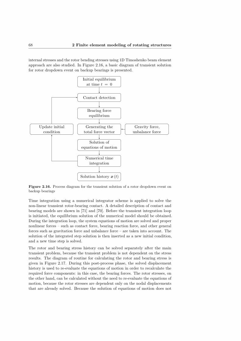
68 2 Finite element modeling of rotating structures
internal stresses and the rotor bending stresses using 1D Timoshenko beam elementapproach are also studied. In Figure 2.16, a basic diagram of transient solutionfor rotor dropdown event on backup bearings is presented.
Initial equilibriumat time t = 0
Contact detection
Bearing forceequilibrium
Generating thetotal force vector
Solution ofequations of motion
Numerical timeintegration
Update initialcondition
Gravity force,unbalance force
Solution history x (t)
Figure 2.16. Process diagram for the transient solution of a rotor dropdown event onbackup bearings
Time integration using a numerical integrator scheme is applied to solve thenon-linear transient rotor-bearing contact. A detailed description of contact andbearing models are shown in [71] and [70]. Before the transient integration loopis initiated, the equilibrium solution of the numerical model should be obtained.During the integration loop, the system equations of motion are solved and propernonlinear forces – such as contact force, bearing reaction force, and other generalforces such as gravitation force and unbalance force – are taken into account. Thesolution of the integrated step solution is then inserted as a new initial condition,and a new time step is solved.The rotor and bearing stress history can be solved separately after the maintransient problem, because the transient problem is not dependent on the stressresults. The diagram of routine for calculating the rotor and bearing stress isgiven in Figure 2.17. During this post-process phase, the solved displacementhistory is used to re-evaluate the equations of motion in order to recalculate therequired force components: in this case, the bearing forces. The rotor stresses, onthe other hand, can be calculated without the need to re-evaluate the equations ofmotion, because the rotor stresses are dependent only on the nodal displacementsthat are already solved. Because the solution of equations of motion does not

2.3 Solution methods 69
Solution of transientproblem x(t)
Update stepsolution x(ti)
Re-evaluate theequations of motion
Retrieve bearingforces F brg
Bearing stresscalculation
σbrg = f (F brg)
Rotor stresscalculation
σrotor = f (x (ti))
Store bearingstress step results
Store rotor stressstep results
Figure 2.17. Process diagram for calculating the rotor and bearing stress history
require evaluation of the rotor stress calculation function, it can be omitted duringtransient solution. The equations for rotor stress calculation are provided in [90],and the equations for bearing stress calculation in [71].

70 2 Finite element modeling of rotating structures
Chapter 3Studies of rotating structures
In this chapter, transient beam element-based rotor dropdown simulation and theresults of rotor and bearing stress history are presented. The correction of beamelement-based rotor model properties using experimental modal data is presented.3D solid element modeling is utilized for studying rotors having contacts. Thenumerical results of shrink-fitted joint behavior are verified using the experimentalmodal analysis results from manufactured test shafts. The results of transientthermal mechanical stress and fatigue analysis of a rotor of a traction motor usingmeasured drive cycle data are presented. As introduced, all the numerical studiesin this chapter utilize measured data. A comprehensive theory of structuraland heat transfer finite element modeling introduced in Chapter 2 is utilized forgenerating the results presented in this chapter, including the solution routinesand contact modeling introduced in Sections 2.3 and 2.2.5.
3.1 Rotor dropdown simulation
Rotor dropdown is an event when AMB-supported rotating machinery experiencesa failure in the AMB control system. In the worst case scenario, the magneticlevitation field collapses and the rotor start to fall free. AMB-supported machineryis, by default, equipped with backup bearings, which will catch the falling rotorand prevent possible catastrophic rotor-stator contact from happening. Thissecondary bearing system will support the rotor during emergency shutdown. Inthis section, the rotor dropdown event on backup bearings is studied. These resultsare based on [90]. Rotor models are generated using the Timoshenko beam elementapproach for its good compatibility as computational speed for transient analysispurposes. Angular acceleration dependent effects according to Equation (2.1) areneglected. The stress state of a flexible rotor during dropdown is calculated, asbased on the previously solved displacement history. In addition, backup bearingHertzian stress history is calculated as a post-process by re-evaluating the systemequations of motion. Both of these stress calculation routines are provided inSection 2.3.4.
71
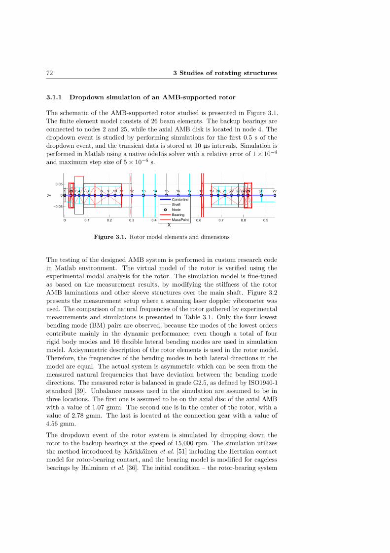
72 3 Studies of rotating structures
3.1.1 Dropdown simulation of an AMB-supported rotor
The schematic of the AMB-supported rotor studied is presented in Figure 3.1.The finite element model consists of 26 beam elements. The backup bearings areconnected to nodes 2 and 25, while the axial AMB disk is located in node 4. Thedropdown event is studied by performing simulations for the first 0.5 s of thedropdown event, and the transient data is stored at 10 µs intervals. Simulation isperformed in Matlab using a native ode15s solver with a relative error of 1× 10⁻⁴
and maximum step size of 5× 10⁻⁶ s.
0 0.1 0.2 0.3 0.4 0.5 0.6 0.7 0.8 0.9
−0.05
0
0.05
S
2726312925242322212019181716
X
POCSBackupSBearingStest
1514131211109876543302821
Y
Centerline
Shaft
Node
Bearing
MassPoint
Figure 3.1. Rotor model elements and dimensions
The testing of the designed AMB system is performed in custom research codein Matlab environment. The virtual model of the rotor is verified using theexperimental modal analysis for the rotor. The simulation model is fine-tunedas based on the measurement results, by modifying the stiffness of the rotorAMB laminations and other sleeve structures over the main shaft. Figure 3.2presents the measurement setup where a scanning laser doppler vibrometer wasused. The comparison of natural frequencies of the rotor gathered by experimentalmeasurements and simulations is presented in Table 3.1. Only the four lowestbending mode (BM) pairs are observed, because the modes of the lowest orderscontribute mainly in the dynamic performance; even though a total of fourrigid body modes and 16 flexible lateral bending modes are used in simulationmodel. Axisymmetric description of the rotor elements is used in the rotor model.Therefore, the frequencies of the bending modes in both lateral directions in themodel are equal. The actual system is asymmetric which can be seen from themeasured natural frequencies that have deviation between the bending modedirections. The measured rotor is balanced in grade G2.5, as defined by ISO1940-1standard [39]. Unbalance masses used in the simulation are assumed to be inthree locations. The first one is assumed to be on the axial disc of the axial AMBwith a value of 1.07 gmm. The second one is in the center of the rotor, with avalue of 2.78 gmm. The last is located at the connection gear with a value of4.56 gmm.The dropdown event of the rotor system is simulated by dropping down therotor to the backup bearings at the speed of 15,000 rpm. The simulation utilizesthe method introduced by Kärkkäinen et al. [51] including the Hertzian contactmodel for rotor-bearing contact, and the bearing model is modified for cagelessbearings by Halminen et al. [36]. The initial condition – the rotor-bearing system
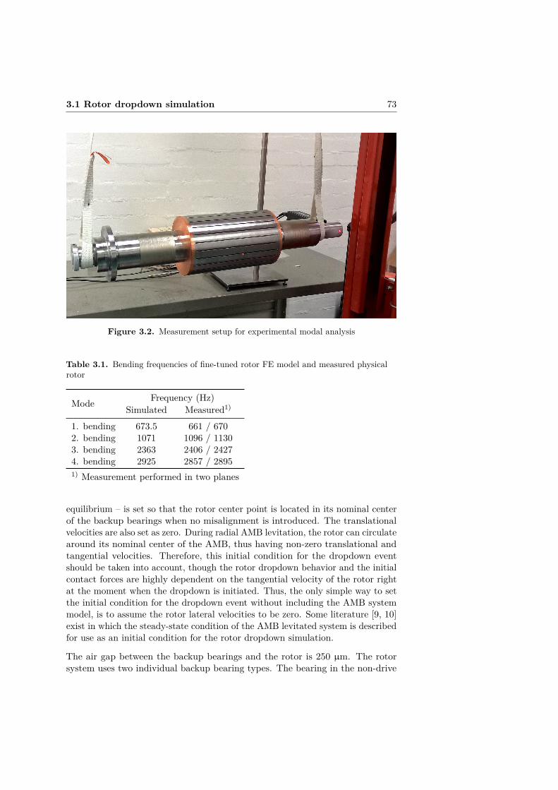
3.1 Rotor dropdown simulation 73
Figure 3.2. Measurement setup for experimental modal analysis
Table 3.1. Bending frequencies of fine-tuned rotor FE model and measured physicalrotor
Mode Frequency (Hz)Simulated Measured1)
1. bending 673.5 661 / 6702. bending 1071 1096 / 11303. bending 2363 2406 / 24274. bending 2925 2857 / 28951) Measurement performed in two planes
equilibrium – is set so that the rotor center point is located in its nominal centerof the backup bearings when no misalignment is introduced. The translationalvelocities are also set as zero. During radial AMB levitation, the rotor can circulatearound its nominal center of the AMB, thus having non-zero translational andtangential velocities. Therefore, this initial condition for the dropdown eventshould be taken into account, though the rotor dropdown behavior and the initialcontact forces are highly dependent on the tangential velocity of the rotor rightat the moment when the dropdown is initiated. Thus, the only simple way to setthe initial condition for the dropdown event without including the AMB systemmodel, is to assume the rotor lateral velocities to be zero. Some literature [9, 10]exist in which the steady-state condition of the AMB levitated system is describedfor use as an initial condition for the rotor dropdown simulation.
The air gap between the backup bearings and the rotor is 250 µm. The rotorsystem uses two individual backup bearing types. The bearing in the non-drive
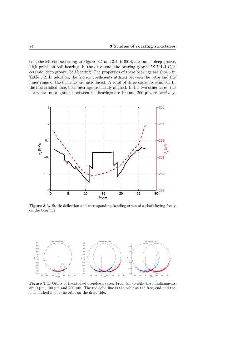
74 3 Studies of rotating structures
end, the left end according to Figures 3.1 and 3.2, is 6014, a ceramic, deep groove,high-precision ball bearing. In the drive end, the bearing type is 5S-7914UC, aceramic, deep groove, ball bearing. The properties of these bearings are shown inTable 3.2. In addition, the friction coefficients utilized between the rotor and theinner rings of the bearings are introduced. A total of three cases are studied. Inthe first studied case, both bearings are ideally aligned. In the two other cases, thehorizontal misalignment between the bearings are 100 and 200 µm, respectively.
0 5 10 15 20 25 30−2
−1.2
−0.4
0.4
1.2
2
σ y [MP
a]
0 5 10 15 20 25 30−265
−263
−261
−259
−257
−255
Uy [µ
m]
Node
Figure 3.3. Static deflection and corresponding bending stress of a shaft laying freelyon the bearings
−300 −200 −100 0 100 200 300−300
−250
−200
−150
−100
−50
0
50
100
150
200
250
Z (µm)
Y (
µm)
Orbit at bearing 1 and 2
−200 −100 0 100 200 300 400
−300
−250
−200
−150
−100
−50
0
50
100
150
200
250
Z (µm)
Y (
µm)
Orbit at bearing 1 and 2
−200 −100 0 100 200 300 400
−300
−200
−100
0
100
200
Z (µm)
Y (
µm)
Orbit at bearing 1 and 2
Figure 3.4. Orbits of the studied dropdown cases. From left to right the misalignmentsare 0 µm, 100 µm and 200 µm. The red solid line is the orbit at the free, end and theblue dashed line is the orbit on the drive side.

3.1 Rotor dropdown simulation 75
Table 3.2. Backup bearing properties
Property 6014 5S-7914UCOuter diameter (mm) 110 110Bore diameter (mm) 70 70Pitch diameter (mm) 90 85Width (mm) 20 16Ball diameter (mm) 12 11.7Number of balls 11 11Static load rating (N) 31.0× 10³ 20.9× 10³
Damping coefficient (Ns/mm) 0.30 0.27Internal clearance (mm) 15× 10−3 9.0× 10⁻³
Conformity ratio in 0.52 0.52Conformity ratio out 0.52 0.52Static friction factor 0.11Kinetic friction factor 0.05
3.1.2 Rotor stresses during dropdown event
Figure 3.4 shows the orbits of the rotor in dropdown. The orbits of all thestudied cases are presented. As seen in Figure 3.4, the misalignment between thebearings greatly affect the behavior of the rotor after the dropdown. With thebearing completely aligned, the rotor bounces after the first contact, but afterthat it settles relatively fast at the bottom of the backup bearing inner rings. Themisalignment of the bearings causes high oscillation behavior in the bottom ofthe bearing inner rings. The orbits in misaligned cases reach to the initial dropheight in the vertical direction.Figure 3.3 presents deflection and the bending stresses of the rotor during staticequilibrium on the backup bearings. The mass of the rotor is not distributedevenly on the bearings at nodes 2 and 25, and the stiffness of the bearing on theother side is lower. Therefore, the displacement of the shaft at the locations ofthe bearing nodes is not equal.
Table 3.3. Comparison of maximum rotor stress components with variousmisalignments during dropdown
Misalignment Stress component (MPa)σy σz τxy τxz
0 µm 6.86 0.73 0.88 0.07100 µm 8.78 2.25 0.75 0.19200 µm 7.54 3.58 0.70 0.36
In Figures 3.5–3.8, the bending and shear stress behavior along the rotational axisby varying the horizontal misalignment of backup bearings is illustrated. Theselection of the simulation results at the particular time is based on the maximum
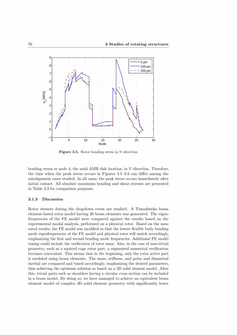
76 3 Studies of rotating structures
0 5 10 15 20 25 30−1
0
1
2
3
4
5
6
7
8
9
Node
σ y [MP
a]
0 µm100 µm200 µm
Figure 3.5. Rotor bending stress in Y -direction
bending stress at node 4, the axial AMB disk location, in Y -direction. Therefore,the time when the peak stress occurs in Figures 3.5–3.8 can differ among themisalignment cases studied. In all cases, the peak stress occurs immediately afterinitial contact. All absolute maximum bending and shear stresses are presentedin Table 3.3 for comparison purposes.
3.1.3 Discussion
Rotor stresses during the dropdown event are studied. A Timoshenko beamelement-based rotor model having 26 beam elements was generated. The eigen-frequencies of the FE model were compared against the results based on theexperimental modal analysis, performed on a physical rotor. Based on the mea-sured results, the FE model was modified so that the lowest flexible body bendingmode eigenfrequencies of the FE model and physical rotor will match accordingly,emphasizing the first and second bending mode frequencies. Additional FE modeltuning could include the verification of rotor mass. Also, in the case of non-trivialgeometry, such as a squirrel cage rotor part, a segmented numerical verificationbecomes convenient. This means that in the beginning, only the rotor active partis modeled using beam elements. The mass, stiffness, and polar and diametralinertial are compared and tuned accordingly, emphasizing the desired parameters,thus achieving the optimum solution as based on a 3D solid element model. Afterthis, trivial parts such as shoulders having a circular cross section can be includedin a beam model. By doing so, we have managed to achieve an equivalent beamelement model of complex 3D solid element geometry with significantly lower

3.1 Rotor dropdown simulation 77
0 5 10 15 20 25 30−1
−0.5
0
0.5
1
1.5
2
2.5
3
3.5
4
Node
σ z [MP
a]
0 µm100 µm200 µm
Figure 3.6. Rotor bending stress in Z-direction
computational requirements. In this studied rotor dropdown case, the rotorgeometry modeled is axisymmetric, though, as introduced, the physical rotor isasymmetric. This asymmetry is due to the squirrel cage part of the rotor assembly.This is clearly visible in the EMA results in Table 3.1. Including this asymmetriceffect requires the use of beam element formulated with inclusion of asymmetriccross section of element.The static equilibrium of the rotor-backup bearing system is presented in Figure 3.3.The shape of the deflection and corresponding bending stress on the outersurface of the rotor are included. The absolute maximum rotor bending stress isapproximately 1.6 MPa. This value is less that one-fifth of the maximum stresspeak recorded during the dropdown event. This finding emphasizes how significantshifting in rotor bending stresses are, occurring after the dropdown has begun.It can be seen that the difference of the cross section changes the stress distributionalong the length of the rotor. Naturally, by changing the cross section properties,the stiffness of the rotor sections will change. Also, the change in diameter changesthe distance of the observed point from the centerline, which exerts a direct impacton the stress results. Bending stresses at both ends of the rotor are zero. Thebending stresses are low, due to the stiff cross section In the mid-section, wherethe active part of the electric machine is located.The bending and shear stress behavior along the rotational axis having variedhorizontal misalignment of the backup bearings is illustrated in Figures 3.5–3.8.By increasing the horizontal misalignment of the backup bearing, bending stressin the Y -direction in the vertical, gravitational direction will increase, as shown
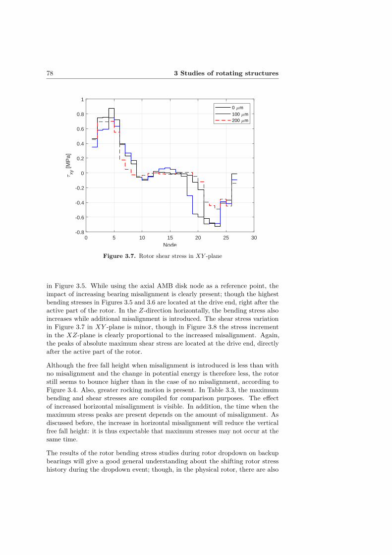
78 3 Studies of rotating structures
0 5 10 15 20 25 30
Node
-0.8
-0.6
-0.4
-0.2
0
0.2
0.4
0.6
0.8
1
xy [M
Pa]
0 m100 m200 m
Figure 3.7. Rotor shear stress in XY -plane
in Figure 3.5. While using the axial AMB disk node as a reference point, theimpact of increasing bearing misalignment is clearly present; though the highestbending stresses in Figures 3.5 and 3.6 are located at the drive end, right after theactive part of the rotor. In the Z-direction horizontally, the bending stress alsoincreases while additional misalignment is introduced. The shear stress variationin Figure 3.7 in XY -plane is minor, though in Figure 3.8 the stress incrementin the XZ-plane is clearly proportional to the increased misalignment. Again,the peaks of absolute maximum shear stress are located at the drive end, directlyafter the active part of the rotor.
Although the free fall height when misalignment is introduced is less than withno misalignment and the change in potential energy is therefore less, the rotorstill seems to bounce higher than in the case of no misalignment, according toFigure 3.4. Also, greater rocking motion is present. In Table 3.3, the maximumbending and shear stresses are compiled for comparison purposes. The effectof increased horizontal misalignment is visible. In addition, the time when themaximum stress peaks are present depends on the amount of misalignment. Asdiscussed before, the increase in horizontal misalignment will reduce the verticalfree fall height: it is thus expectable that maximum stresses may not occur at thesame time.
The results of the rotor bending stress studies during rotor dropdown on backupbearings will give a good general understanding about the shifting rotor stresshistory during the dropdown event; though, in the physical rotor, there are also

3.2 Bearing stress simulation 79
0 5 10 15 20 25 30
Node
-0.4
-0.3
-0.2
-0.1
0
0.1
0.2
0.3
xz [M
Pa]
0 m100 m200 m
Figure 3.8. Rotor shear stress in XZ-plane
other stress sources present. The general stress state caused by the centrifugal forcehas significantly greater amplitude than the bending stresses, due to rotor contacton backup bearings as predicted using the beam element method. In addition,contact between other components, especially if shrink fitted joints are used, willyield high stress amplitudes. Thus, a physical rotor will experience significantlygreater stresses even during normal use and even greater stresses during dropdown.When these speed and joint dependent stresses introduced are included in analysisby using the 3D solid element approach, the stress-stiffening effect should betaken into account. This effect can stiffen the rotor, and can have an effect onthe rotor bending amplitude during the dropdown event. Regardless, the beamelement approach for the rotor dropdown event is very useful for determining therotor deformations. This information is essential for rotor-stator clearance design,especially in a case of overhung impeller.
3.2 Bearing stress simulation
An AMB-supported rotor system with backup bearing is studied in order toinvestigate the backup bearing stress history. The importance of analyzing thestresses that backup bearing experiences arises from the typical, often chaotic,nature of the dropdown event. During dropdown of a rotor of a high-speed motor,the bearing forces can be many times greater than during operation lower speedoperation, when the connection between the rotor and bearing inner ring hasno clearance. Because of the required operational air gap between rotor and
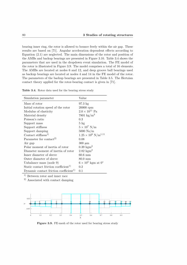
80 3 Studies of rotating structures
bearing inner ring, the rotor is allowed to bounce freely within the air gap. Theseresults are based on [71]. Angular acceleration dependent effects according toEquation (2.1) are neglected. The main dimensions of the rotor and position ofthe AMBs and backup bearings are presented in Figure 3.10. Table 3.4 shows theparameters that are used in the dropdown event simulation. The FE model ofthe rotor is illustrated in Figure 3.9. The model comprises a total of 16 elements.The AMBs are located at nodes 6 and 12, and deep groove ball bearings usedas backup bearings are located at nodes 4 and 14 in the FE model of the rotor.The parameters of the backup bearings are presented in Table 3.5. The Hertziancontact theory applied for the rotor-bearing contact is given in [71].
Table 3.4. Rotor data used for the bearing stress study
Simulation parameter ValueMass of rotor 97.3 kgInitial rotation speed of the rotor 20000 rpmModulus of elasticity 2.0× 10¹¹ PaMaterial density 7801 kg/m3
Poisson’s ratio 0.3Support mass 5 kgSupport stiffness 5× 10⁷ N/mSupport damping 5000 Ns/mContact stiffness1) 1.25× 10⁹ N/m1.11
Parameter for contact2) 0.08Air gap 300 µmPolar moment of inertia of rotor 0.39 kgm2
Diameter moment of inertia of rotor 2.82 kgm2
Inner diameter of sleeve 60.6 mmOuter diameter of sleeve 80.0 mmUnbalance mass (node 9) 6× 10⁵ kgm at 0Static contact friction coefficient1) 0.2Dynamic contact friction coefficient1) 0.11) Between rotor and inner race2) Associated with contact damping
0 0.1 0.2 0.3 0.4 0.5 0.6 0.7 0.8 0.9
X
-0.05
0
0.05
Y
1387 1021 149 125 174 11 15 163 6
Figure 3.9. FE-mesh of the rotor used for bearing stress study

3.2 Bearing stress simulation 81
The dropdown event is simulated for 1 s, and the simulation time step is 10 µs.The equations of motion are time-integrated using Matlab ode45. The relativeerror and maximum step size are equal to 1× 10⁻⁵ and 10 µs, respectively.
990.0
90.0
370.0
115.0 105.0 257.5
A M BU B
195
.0
Y
X
475.0
80
.0
165.0
60
.0
5
0.0
660.0
TB
Figure 3.10. Main dimensions of the rotor model used for bearing stress study
Table 3.5. 6016 deep groove ball bearing properties used for the bearing stress study
Bearing parameter ValueBearing damping coefficient 0.25 Ns/mmBearing diametric clearance 15 µmOuter diameter 125 mmBall diameter 19.05 mmPitch diameter 110 mmBore diameter 80 mmModulus of elasticity of ball 2× 10¹¹ PaModulus of elasticity of inner race 2× 10¹¹ PaPoisson’s ratio of ball 0.3Poisson’s ratio of inner race 0.3Conformity ratio 0.52Number of balls 10
3.2.1 Stress in a backup bearing during dropdown
In the simulation, the penetration of the ball in the inner race is calculatedfrom the relative displacements between the inner and outer races. Figure 3.11illustrates the orbit of rotor during the dropdown. In this figure, the dashed line

82 3 Studies of rotating structures
shows the air gap and the solid line shows the path of the rotor center point atthe bearing location during the dropdown event. After the first contact betweenthe rotor and bearing, the rotor bounces, after which it settles steadily on thebottom of the inner race.
-3-2-10123Z [m] 10-4
-3
-2
-1
0
1
2
3
Y [
m]
10-4
Figure 3.11. Orbit of the rotor during the dropdown event
2
34
5
7
8 9
10
6 1
Figure 3.12. Ball arrangement at the start of the simulation

3.2 Bearing stress simulation 83
0 0.05 0.1 0.15 0.2 0.25 0.3Time [s]
0
0.5
1
1.5
2
2.5
3
3.5
4
Dis
plac
emen
t [m
]
10-4
relative displacment ofrotor and inner race
air gap
contacts
Figure 3.13. Relative displacement of the rotor and the inner race
Figure 3.14. Maximum Hertzian stress of each ball
Figure 3.13 shows the relative displacement of the rotor and inner race as afunction of time. The first contact of the rotor and backup bearing occurs 8.98 msafter the dropdown is initiated. Duration of this contact is approximately 2 ms;

84 3 Studies of rotating structures
after that, the rotor bounces back. The rotor contacts the inner race for thesecond time at 20.5 ms. After the third contact, at 27.06 ms, the rotor and innerrace remain in continuous contact.Figure 3.14 shows the stress history for the contact of each ball and the inner race.The theory for calculating the Hertzian contact stress is given in [71]. The stresshistory shows that the stresses are not uniformly distributed among the balls.After the first contact, the backup bearing experiences the highest contact stressof 2014 MPa. Then, the stresses decline and the differences in the stresses amongthe balls gradually decreases as the inner ring starts to rotate. The maximumHertzian contact stress is experienced in the ball number 8, which was initiallysituated at 252 (Figure 3.12).
200
400
600
800
30
210
60
240
90
270
120
300
150
330
180 0
ball 9, 762 Nball 8, 794 N
ball 7, 241 N ball 10, 185 N
(a)
1000
2000
3000
30
210
60
240
90
270
120
300
150
330
180 0
ball 10, 1240 MPaball 7, 1353 MPa
ball 9, 1986 MPaball 8, 2014 MPa
(b)
Figure 3.15. Distribution of load (a) and stress (b) in the backup bearing during thefirst contact
Figure 3.15 depicts the distribution of the load and the stress during the firstcontact of the rotor and the backup bearing. The maximum Hertzian stressdistribution in second and third contact of the rotor and inner race is depicted inFigure 3.16.
3.2.2 Discussion
The backup bearing experiences the highest Hertzian stress directly after theinitial rotor-bearing contact during the dropdown event. The bearing stress is notuniform during the first contact at the beginning of the simulation. The reason forthis is that only a few balls are at the loaded zone during the first rotor-bearingcontact. The loaded zone is formed by the ball under the horizontal center of thebearing (balls 7–10 according to Figure 3.12). In addition, the deep groove ballbearings have minor internal clearance, which contributes to the contact forcedistribution between an individual ball and the rings inside the bearing.

3.2 Bearing stress simulation 85
30
210
60
240
90
270
120
300
150
330
180 0
ball 8, 1707 MPa
ball 9, 1226 MPa
ball 6, 595 MPa
ball 7, 1578 MPa
(a)
30
210
60
240
90
270
120
300
150
330
180 0
ball 8, 1588 MPa
ball 9, 852 MPa
ball 6, 923 MPa
ball 7, 1601MPa
(b)
Figure 3.16. Maximum Hertzian stress distribution in the second (a) and third (b)contact of the rotor with the inner race
The distribution of the load and the stress during the first rotor-bearing contact isshown in Figure 3.15. During the first contact, the balls numbered 7–10 penetratethe inner race as in Figure 3.12. The locations of these balls are at phase angles216, 252, 288 and 324. The highest calculated stress is found in the contactbetween ball number 8 and the inner race, where the maximum contact forceof 794 N is present, and the maximum Hertzian stress is 2014 MPa. The totalcontact force between the rotor and inner race has two components during thefirst contact of the rotor with the backup bearing. The vertical force componentis due to gravitational force of the rotor weight. Because of the frictional contact,the friction force between the rotor and inner race is in the horizontal directionacting in the opposite direction to the rotation of the rotor. Therefore, the totalcontact force vector is pointing to the left towards ball number 8 (Figure 3.12).
Figure 3.16 presents the maximum Hertzian stress distribution of second andthird contact of the rotor and inner race. During the second and third contacts,ball number 10 moved away from the loaded zone, and was no longer in contactwith the inner race. Also, the location of the balls changed due to the frictionforce-induced acceleration of the inner ring. In the second contact, balls 6–9 wereat 185, 221, 257, and 293 phase angles, respectively, according to Figure 3.16a;and ball number 8 experienced the highest stress. In the third contact, balls6, 7, 8 and 9 moved to 191, 227, 263 and 299 phase angles, according toFigure 3.16b; the highest stress was found in the contact between ball number 7and the inner race. The simulation reveals that different balls were in contact withthe inner race at various times as the bearing inner ring accelerated, due to thefrictional forces induced by the rotor-bearing contact during the rotor dropdownevent. Furthermore, the stress magnitude and the location of the ball with the

86 3 Studies of rotating structures
highest stress changed due to the rotation of inner ring and consequently due tothe rotation of the balls in the bearing.
3.3 Rotors with internal contacts
Studies in this section are based on the use of the 3D solid element modelingapproach for rotors having contacts. These results are based on [91]. Theexperimental results of manufactured test shafts having shrink-fitted joints arecompared against the results generated using the proposed contact modelingmethod given in Section 2.2.5. The accuracy the constraint equation methodsused for contact modeling between two solid bodies as well as the boundaryconstraints are presented and discussed. The solution routine for generatinga Campbell diagram for a rotor having contact introduced in Section 2.3.1 isutilized for studying a shrink-fitted conical impeller-shaft contact and its dynamicbehavior under centrifugal loads.
3.3.1 Experimental results of test shaft assembly
The test shaft assembly under investigation consists of a steel shaft and shrink-fitted aluminum sleeve, as shown in Figure 3.17. Certain material properties ofindividual components are verified by measuring mass properties and the lowestfree-free natural bending mode frequencies (shafts only). For shrink-fitted jointtesting purposes, three sets of test shaft assemblies are made with varying radialinterferences, and then measured by means of experimental modal analysis. Ascanning laser doppler vibrometer is used for modal analysis, which providescontactless measurement and does not require sensors that would add mass onthe test pieces. The experimental results are shown in Table 3.6. Based on themeasured first free-free natural bending frequencies, the radial interference in theshrink fit joint does not exert a significant effect on the natural frequencies of thetest assemblies.
Table 3.6. Experimental results of various radial interferences of test shaft assemblies
Radial1. BM (Hz) 2. BM (Hz)Test shaft interference
assembly δrad (µm)1 3.0 1105.9 3084.02 9.0 1108.2 3098.43 14 1108.6 3095.7Average 1107.6 3092.7Difference +0.09 % / +0.18 % /(max/min)1) -0.15 % -0.28 %1) Max/min value compared against the correspondingaveraged value
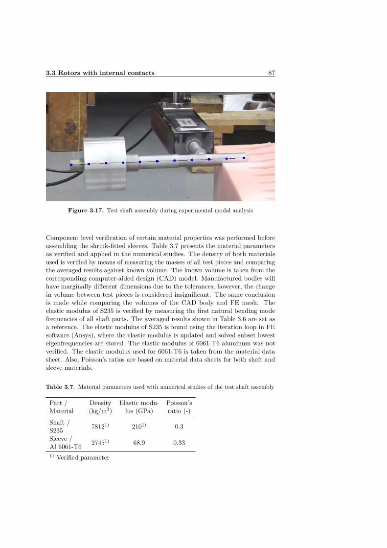
3.3 Rotors with internal contacts 87
Figure 3.17. Test shaft assembly during experimental modal analysis
Component level verification of certain material properties was performed beforeassembling the shrink-fitted sleeves. Table 3.7 presents the material parametersas verified and applied in the numerical studies. The density of both materialsused is verified by means of measuring the masses of all test pieces and comparingthe averaged results against known volume. The known volume is taken from thecorresponding computer-aided design (CAD) model. Manufactured bodies willhave marginally different dimensions due to the tolerances; however, the changein volume between test pieces is considered insignificant. The same conclusionis made while comparing the volumes of the CAD body and FE mesh. Theelastic modulus of S235 is verified by measuring the first natural bending modefrequencies of all shaft parts. The averaged results shown in Table 3.6 are set asa reference. The elastic modulus of S235 is found using the iteration loop in FEsoftware (Ansys), where the elastic modulus is updated and solved subset lowesteigenfrequencies are stored. The elastic modulus of 6061-T6 aluminum was notverified. The elastic modulus used for 6061-T6 is taken from the material datasheet. Also, Poisson’s ratios are based on material data sheets for both shaft andsleeve materials.
Table 3.7. Material parameters used with numerical studies of the test shaft assembly
Part / Density Elastic modu- Poisson’sMaterial (kg/m3) lus (GPa) ratio (-)Shaft / 78121) 2101) 0.3S235Sleeve / 27451) 68.9 0.33Al 6061-T61) Verified parameter

88 3 Studies of rotating structures
3.3.2 Numerical results of test shaft assembly
Based on the measured results of manufactured test shaft assemblies, the shrinkfit interference seems to have a minor impact on the free-free natural bendingfrequencies. Therefore, the case of 3 µm interference is selected for numericalstudies. The FE mesh of the test shaft assembly used in the numerical studiesis presented in Figure 3.18. The mesh generator in Ansys Mechanical is usedfor generating the FE mesh. The mesh consists of 36,838 ten-node quadratictetrahedron elements. By using a mesh imported from Ansys, possible differencesof model discretization are avoided, and differences between the two modelingapproaches are thereby minimized. The main dimensions of the test shaft assemblyare presented in Figure 3.19. The mesh size at the contact zone is 2.5 mm.
Figure 3.18. FE mesh of test shaft assembly
260
18
(20) 60
20
80
26
20
18
20 60 100
A A
B B
C C
D D
E E
F F
4
4
3
3
2
2
1
1
DRAWN
CHK'D
APPV'D
MFG
Q.A
UNLESS OTHERWISE SPECIFIED:DIMENSIONS ARE IN MILLIMETERSSURFACE FINISH:TOLERANCES:
LINEAR:ANGULAR:
FINISH: DEBURR AND BREAK SHARP EDGES
NAME SIGNATURE DATE
MATERIAL:
DO NOT SCALE DRAWING REVISION
TITLE:
DWG NO.
SCALE:1:5 SHEET 1 OF 1
A4
WEIGHT:
dummy_shaft_end_assembly_HA
Figure 3.19. Main dimensions of test shaft assembly
The numerical results are obtained using the proposed solution routine for solvingthe eigenfrequencies for a rotor having contacts and using the developed customtrial force constraint equation method. For comparison purposes, commercial
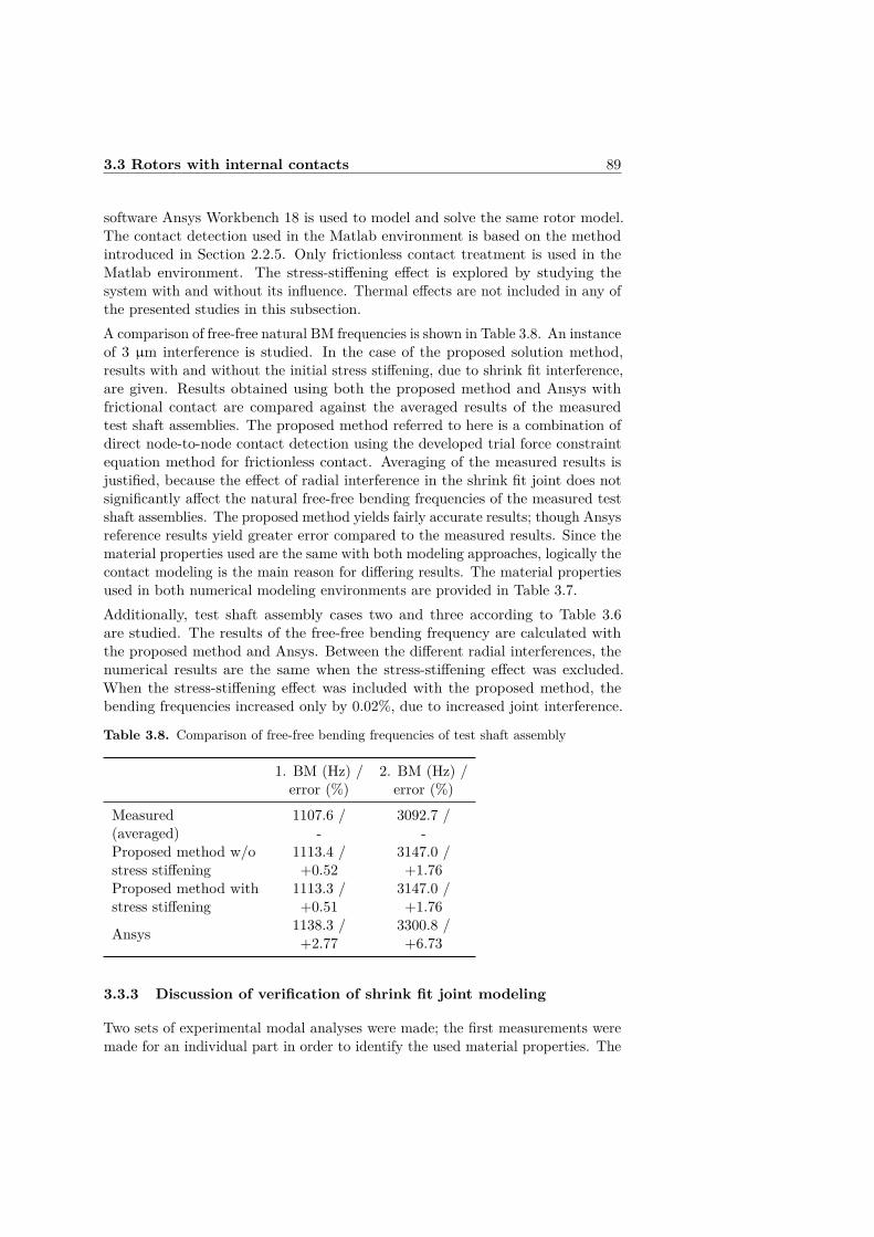
3.3 Rotors with internal contacts 89
software Ansys Workbench 18 is used to model and solve the same rotor model.The contact detection used in the Matlab environment is based on the methodintroduced in Section 2.2.5. Only frictionless contact treatment is used in theMatlab environment. The stress-stiffening effect is explored by studying thesystem with and without its influence. Thermal effects are not included in any ofthe presented studies in this subsection.A comparison of free-free natural BM frequencies is shown in Table 3.8. An instanceof 3 µm interference is studied. In the case of the proposed solution method,results with and without the initial stress stiffening, due to shrink fit interference,are given. Results obtained using both the proposed method and Ansys withfrictional contact are compared against the averaged results of the measuredtest shaft assemblies. The proposed method referred to here is a combination ofdirect node-to-node contact detection using the developed trial force constraintequation method for frictionless contact. Averaging of the measured results isjustified, because the effect of radial interference in the shrink fit joint does notsignificantly affect the natural free-free bending frequencies of the measured testshaft assemblies. The proposed method yields fairly accurate results; though Ansysreference results yield greater error compared to the measured results. Since thematerial properties used are the same with both modeling approaches, logically thecontact modeling is the main reason for differing results. The material propertiesused in both numerical modeling environments are provided in Table 3.7.Additionally, test shaft assembly cases two and three according to Table 3.6are studied. The results of the free-free bending frequency are calculated withthe proposed method and Ansys. Between the different radial interferences, thenumerical results are the same when the stress-stiffening effect was excluded.When the stress-stiffening effect was included with the proposed method, thebending frequencies increased only by 0.02%, due to increased joint interference.
Table 3.8. Comparison of free-free bending frequencies of test shaft assembly
1. BM (Hz) / 2. BM (Hz) /error (%) error (%)
Measured 1107.6 / 3092.7 /(averaged) - -Proposed method w/o 1113.4 / 3147.0 /stress stiffening +0.52 +1.76Proposed method with 1113.3 / 3147.0 /stress stiffening +0.51 +1.76
Ansys 1138.3 / 3300.8 /+2.77 +6.73
3.3.3 Discussion of verification of shrink fit joint modeling
Two sets of experimental modal analyses were made; the first measurements weremade for an individual part in order to identify the used material properties. The

90 3 Studies of rotating structures
second measurements were made for assembled shrink fitted test shaft assembliesto identify the effect of the various radial interferences used. Based on themeasurement results, low radial interferences do not significantly contribute tothe lowest natural bending frequencies of the structures studied. A minor increasein the first bending mode frequencies was observed, according to Table 3.6. Sincethe change in the first bending frequencies was, relatively, fractions of only onepercent, and the frequency increase in second bending modes is inconsistent,these changes can be related to environment factors or the accuracy of the usedmeasurement device. Averaged values of the frequencies of the two lowest bendingmode are thus used for comparison with the numerical results.
All three radial interferences of the test shaft assemblies were numerically studied.When the stress-stiffening effect was excluded, no shifting was observed in thelowest bending mode frequencies. On the other hand, when pre-stress was includedin the eigenvalue analysis, the greatest relative change in the bending frequencieswas only 0.02%. A pre-stress condition can cause an increase in the naturalfrequencies of a structure. However, with these studied test shaft assemblies, theradial interference level is so low that no visible pre-stressed impact is visible.
3.3.4 Accuracy of contact modeling
In this section, the constraint error at the contact region achieved using theproposed contact modeling method with the trial force constraint method ispresented. The constraint error magnitude is relevant in order to achieve convergedresults. Also, the results of the constraint error at the contact region calculatedwith Ansys are presented for comparison purposes. Figure 3.20 introduces thecylindrical constraints that are used as boundary conditions for the contacttreatment with the proposed method. The displacements of the assembly accordingto Figure 3.20 are constrained as follows: radial deformation is allowed whiletangential deformation is restricted. Axial rigid body movement is constrained,but axial deformations are allowed. In Ansys, a corresponding boundary constraintset is modeled using the native Cylindrical constraint tools.
For a reference solution for the constraint error analysis, the test shaft assemblyis selected. Rotational speed is set to be zero in order to ensure that no externalloads are present and that the contact region remains fully closed. The errorof constraint equations at the shrink fitted joint contact region is presented inFigure 3.21. Cylindrical constraints, a set of constraints between the shaft bodyand ground, are used to prevent rigid body motion during the solution of thecontact problem. The cylindrical constraint error is presented in Figure 3.22.
For comparison purposes, the multipoint constraint method, also known as themaster-slave constraint method, is utilized [102]. This particular constraint methodis very effective because it uses the master-slave relation and while removing theslave DOF the solution turn out to be exact. The mean constraint error withthe MPC method at contact region is −7.0304× 10⁻²⁰ m and the cylindricalconstraint mean error is −1.1979× 10⁻²² m.

3.3 Rotors with internal contacts 91
Z
Y
Figure 3.20. Cylindrical constraints applied to the test shaft assembly model: red dotTX = 0 (in the origo), green dots TY = 0, blue dots TZ = 0
For further comparison, two sets of constraint errors at the contact region arecalculated using Ansys. In the first case, the contact formulation used is augmentedLagrangian [103, 104]. The constraint error of this case is presented in Figure 3.23.
−2 −1.5 −1 −0.5 0 0.5 1 1.5 2
·10−6
0
100
200
300
Constraint error (m)
Num
berof
node
s
Mean error -3.6468e-07 (m)
Figure 3.23. Constraint error at the contact region using the augmented Lagrangianmethod with Ansys
The other Ansys result set is presented in Figure 3.24. The contact formulationused is normal Lagrangian, which is the traditional Lagrangian method.
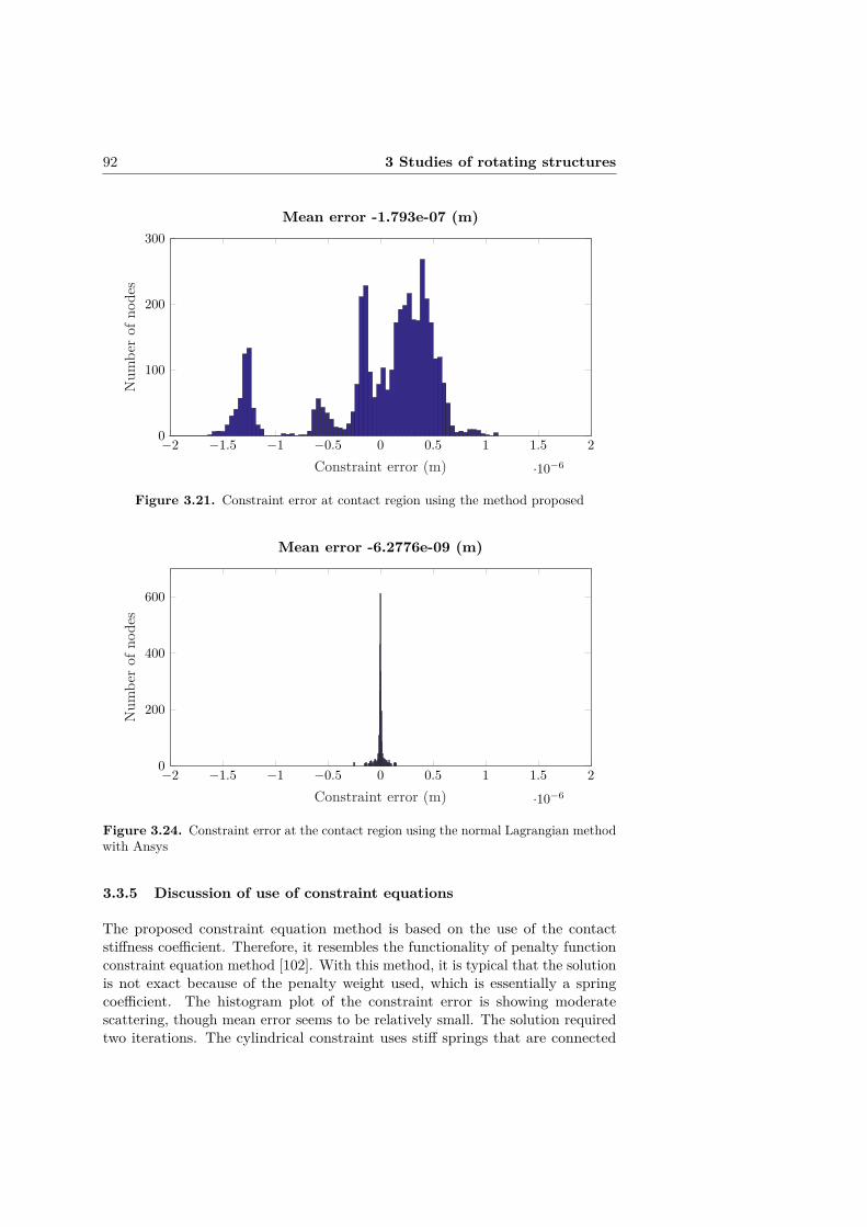
92 3 Studies of rotating structures
−2 −1.5 −1 −0.5 0 0.5 1 1.5 2
·10−6
0
100
200
300
Constraint error (m)
Num
berof
node
s
Mean error -1.793e-07 (m)
Figure 3.21. Constraint error at contact region using the method proposed
−2 −1.5 −1 −0.5 0 0.5 1 1.5 2
·10−6
0
200
400
600
Constraint error (m)
Num
berof
node
s
Mean error -6.2776e-09 (m)
Figure 3.24. Constraint error at the contact region using the normal Lagrangian methodwith Ansys
3.3.5 Discussion of use of constraint equations
The proposed constraint equation method is based on the use of the contactstiffness coefficient. Therefore, it resembles the functionality of penalty functionconstraint equation method [102]. With this method, it is typical that the solutionis not exact because of the penalty weight used, which is essentially a springcoefficient. The histogram plot of the constraint error is showing moderatescattering, though mean error seems to be relatively small. The solution requiredtwo iterations. The cylindrical constraint uses stiff springs that are connected
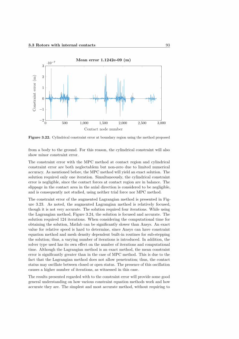
3.3 Rotors with internal contacts 93
0 500 1,000 1,500 2,000 2,500 3,000−2
−1
0
1
2
3·10−7
Contact node number
Con
strainterror(m
)
Mean error 1.1242e-09 (m)
Figure 3.22. Cylindrical constraint error at boundary region using the method proposed
from a body to the ground. For this reason, the cylindrical constraint will alsoshow minor constraint error.The constraint error with the MPC method at contact region and cylindricalconstraint error are both neglectablem but non-zero due to limited numericalaccuracy. As mentioned before, the MPC method will yield an exact solution. Thesolution required only one iteration. Simultaneously, the cylindrical constrainterror is negligible, since the contact forces at contact region are in balance. Theslippage in the contact area in the axial direction is considered to be negligible,and is consequently not studied, using neither trial force nor MPC method.The constraint error of the augmented Lagrangian method is presented in Fig-ure 3.23. As noted, the augmented Lagrangian method is relatively focused,though it is not very accurate. The solution required four iterations. While usingthe Lagrangian method, Figure 3.24, the solution is focused and accurate. Thesolution required 124 iterations. When considering the computational time forobtaining the solution, Matlab can be significantly slower than Ansys. An exactvalue for relative speed is hard to determine, since Ansys can have constraintequation method and mesh density dependent built-in routines for sub-steppingthe solution; thus, a varying number of iterations is introduced. In addition, thesolver type used has its own effect on the number of iterations and computationaltime. Although the Lagrangian method is an exact method, the mean constrainterror is significantly greater than in the case of MPC method. This is due to thefact that the Lagrangian method does not allow penetration; thus, the contactstatus may oscillate between closed or open status. The presence of this oscillationcauses a higher number of iterations, as witnessed in this case.The results presented regarded with to the constraint error will provide some goodgeneral understanding on how various constraint equation methods work and howaccurate they are. The simplest and most accurate method, without requiring to

94 3 Studies of rotating structures
increase the number of DOFs is the MPC method. Although this method requiresa separate transformation matrix to be formulated, it can still be considered to beone of the best constraint methods. In addition, the MPC method yields accurateresults with only one iteration. The Lagrangian method, with and without theaugmented part also requires an additional bordered stiffness matrix. The MPCmethod is also available in Ansys, though it can be used only with contacts thatdo remain closed, bonded and no separation; thus, it cannot be used for frictionalcontact. The most accurate contact option Ansys offers with the least optionsfor tuning for frictional contact is normal Lagrangian; nevertheless, it requires alarge number of iterations to yield accurate results.
3.3.6 Conical impeller assembly
An assembly of a conical impeller shrink-fitted on a shaft is studied. The FEmesh of the conical impeller assembly is presented in Figure 3.25. The meshconsists of 24,766 ten-node quadratic tetrahedron elements. The main dimensionsof the conical impeller assembly are presented in Figure 3.26. The mesh size atthe contact zone is 5.0 mm. The conical impeller of the radial kinetic compressorwheel is simplified and modeled without the blades. Thus, only the hub of theimpeller is included in the FE mesh. By doing so, the FE-problem size can bereduced and the lower number of the lowest eigenmodes utilized by neglecting thelow frequency local bending modes of the impeller blades. The material propertiesused in this study are presented in Table 3.9.
Figure 3.25. FE mesh of conical impeller assembly
Two simple identical bearings, essentially spring-damper elements, are locatedat both ends of the shaft of the conical impeller assembly and connected to thesurfaces of the end planes of the shaft. The stiffness and damping parameters usedare presented in Table 3.10. The studied speed range is from zero to 30,000 rpm,with an increment of 1000 rpm. The radial interference in the conical impeller-shaftshrink fit is 50 µm.
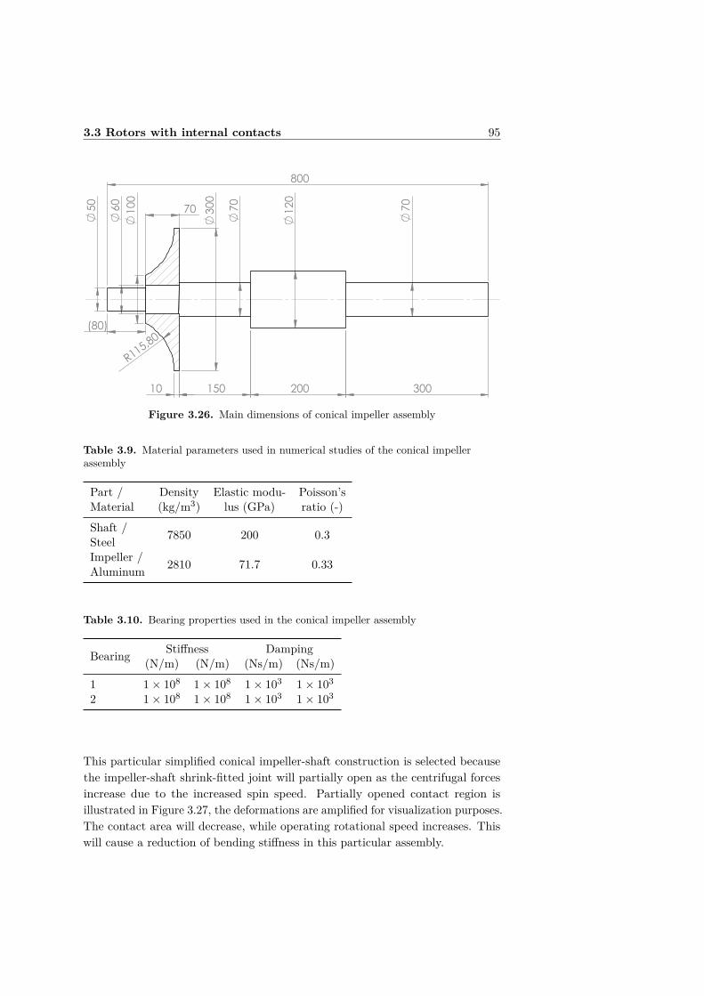
3.3 Rotors with internal contacts 95
R115,80
800
50
300
60
70
120
70
(80)
150 200 300
70
10
100
Figure 3.26. Main dimensions of conical impeller assembly
Table 3.9. Material parameters used in numerical studies of the conical impellerassembly
Part / Density Elastic modu- Poisson’sMaterial (kg/m3) lus (GPa) ratio (-)Shaft / 7850 200 0.3SteelImpeller / 2810 71.7 0.33Aluminum
Table 3.10. Bearing properties used in the conical impeller assembly
Bearing Stiffness Damping(N/m) (N/m) (Ns/m) (Ns/m)
1 1× 10⁸ 1× 10⁸ 1× 10³ 1× 10³
2 1× 10⁸ 1× 10⁸ 1× 10³ 1× 10³
This particular simplified conical impeller-shaft construction is selected becausethe impeller-shaft shrink-fitted joint will partially open as the centrifugal forcesincrease due to the increased spin speed. Partially opened contact region isillustrated in Figure 3.27, the deformations are amplified for visualization purposes.The contact area will decrease, while operating rotational speed increases. Thiswill cause a reduction of bending stiffness in this particular assembly.

96 3 Studies of rotating structures
Closed contactregion Opened contact region
Figure 3.27. Visualization of contact region partial opening between the conical impellerand shaft
Table 3.11. First whirling mode frequencies at 30,000 rpm of the conical impellerassembly
At 30,000 rpm1. BW (Hz) 1. FW (Hz)
Proposed method w/o 161.1 171.1stress stiffeningProposed method with 168.6 176.8stress stiffeningProposed method with 165.5 173.3fixed contactAnsys 166.4 173.9
Campbell diagram of the conical impeller assembly without the stress-stiffeningeffect is presented in Figure 3.28, and the critical speeds of forward whirl (FW)and backward whirl (BW) modes are given. The effect of partially openedcontact is present in the Campbell diagram, as the overall bending stiffness ofthe assembly starts to decline at 15,000 rpm. A Campbell diagram of the conicalimpeller assembly with stress-stiffening effect is presented in Figure 3.29. Thestress-stiffening effect will not yield a significant stiffening effect on the bendingmodes.
For comparison purposes, the Campbell diagram of the conical impeller assemblywith fixed contact is presented in Figure 3.30. The initial interference in theshrink fit joint is not present, and the stress-stiffening effect is neglected. Sincethe contact is fixed, the effect of bending stiffness reduction due to the reduced
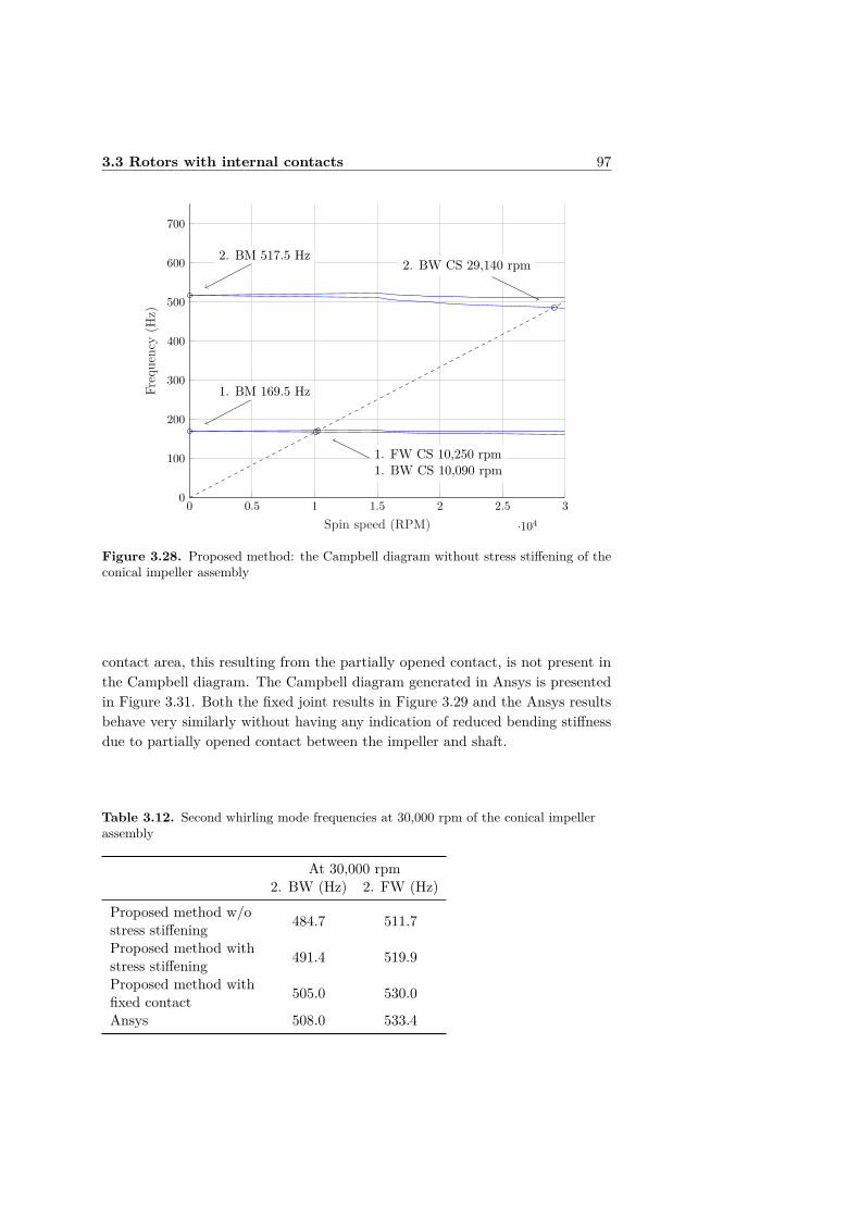
3.3 Rotors with internal contacts 97
0 0.5 1 1.5 2 2.5 3·104
0
100
200
300
400
500
600
700
1. BM 169.5 Hz
2. BM 517.5 Hz
1. FW CS 10,250 rpm1. BW CS 10,090 rpm
2. BW CS 29,140 rpm
Spin speed (RPM)
Frequency(H
z)
Figure 3.28. Proposed method: the Campbell diagram without stress stiffening of theconical impeller assembly
contact area, this resulting from the partially opened contact, is not present inthe Campbell diagram. The Campbell diagram generated in Ansys is presentedin Figure 3.31. Both the fixed joint results in Figure 3.29 and the Ansys resultsbehave very similarly without having any indication of reduced bending stiffnessdue to partially opened contact between the impeller and shaft.
Table 3.12. Second whirling mode frequencies at 30,000 rpm of the conical impellerassembly
At 30,000 rpm2. BW (Hz) 2. FW (Hz)
Proposed method w/o 484.7 511.7stress stiffeningProposed method with 491.4 519.9stress stiffeningProposed method with 505.0 530.0fixed contactAnsys 508.0 533.4
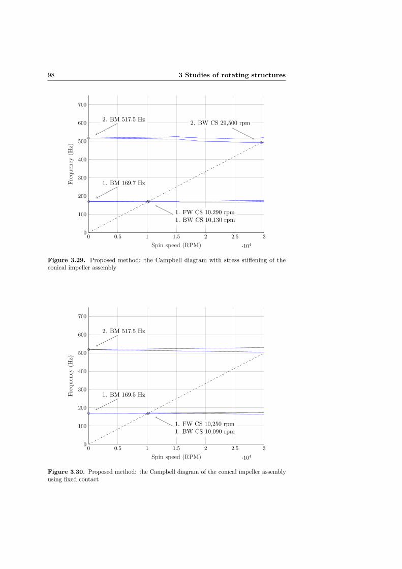
98 3 Studies of rotating structures
0 0.5 1 1.5 2 2.5 3·104
0
100
200
300
400
500
600
700
1. BM 169.7 Hz
2. BM 517.5 Hz
1. FW CS 10,290 rpm1. BW CS 10,130 rpm
2. BW CS 29,500 rpm
Spin speed (RPM)
Frequency(H
z)
Figure 3.29. Proposed method: the Campbell diagram with stress stiffening of theconical impeller assembly
0 0.5 1 1.5 2 2.5 3·104
0
100
200
300
400
500
600
700
1. BM 169.5 Hz
2. BM 517.5 Hz
1. FW CS 10,250 rpm1. BW CS 10,090 rpm
Spin speed (RPM)
Frequency(H
z)
Figure 3.30. Proposed method: the Campbell diagram of the conical impeller assemblyusing fixed contact

3.3 Rotors with internal contacts 99
0 0.5 1 1.5 2 2.5 3·104
0
100
200
300
400
500
600
700
1. BM 170.3 Hz
2. BM 520.9 Hz
1. FW CS 10,300 rpm1. BW CS 10,140 rpm
Spin speed (RPM)
Frequency(H
z)
Figure 3.31. Ansys Campbell diagram of the conical impeller assembly using frictionalcontact
3.3.7 Effect of geometric nonlinearities to the critical speeds
With the conical impeller assembly, the first two bending modes are visible inthe Campbell diagrams (Figures 3.28–3.31). The first BW and FW critical speedof Ansys is consistently 50 rpm greater than the ones with the method beingproposed. In addition, the results obtained using the proposed method with thestress-stiffening effect are actually the same as the Ansys model frequencies. Sincethe contact treatment is applied on every speed step while using the proposedmethod, the contact opening is taken into account. The use of any particularconstraint equation method does not contribute to the contact opening: only theexternal forces – in this particular case, the centrifugal force – will contribute tothe opening of contact. Constraint equations are utilized after the contact statusis solved, and used for the remaining contact area where the contact remainsclosed. Due to reduction in the contact surface area owing to high-speed operation,a dip in the mode lines in the Campbell diagrams (Figures 3.28–3.29) is present.Only the models with frictionless contact using the proposed solution routineexperience the second BW mode in the speed range studied. The stress-stiffeningeffect increases the second BW critical speed by 360 rpm.
The reason for a rather large reduction in whirl mode frequencies of the secondbending mode using frictionless contact is explicable due to the BM shapesof the supported structure. The two lowest zero speed bending modes of thesupported conical impeller assembly are illustrated in Figure 3.32 using Paraviewvisualization software. The node points of the first bending mode are at bearing
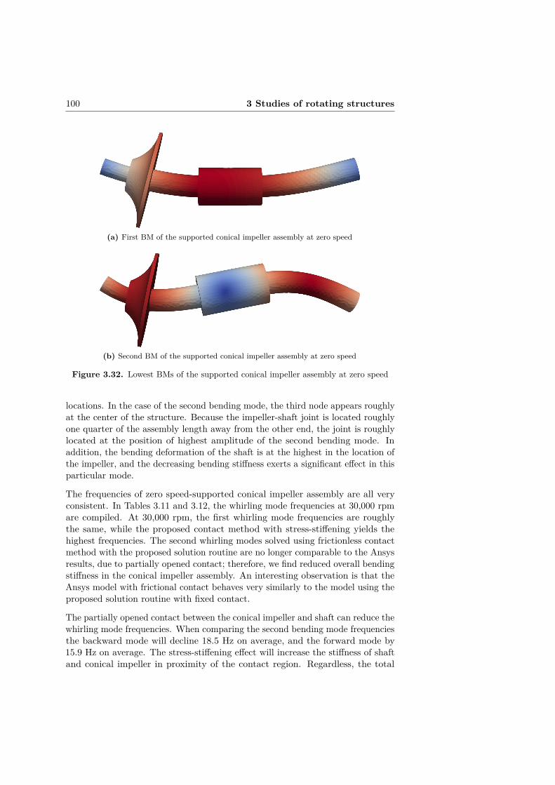
100 3 Studies of rotating structures
(a) First BM of the supported conical impeller assembly at zero speed
(b) Second BM of the supported conical impeller assembly at zero speed
Figure 3.32. Lowest BMs of the supported conical impeller assembly at zero speed
locations. In the case of the second bending mode, the third node appears roughlyat the center of the structure. Because the impeller-shaft joint is located roughlyone quarter of the assembly length away from the other end, the joint is roughlylocated at the position of highest amplitude of the second bending mode. Inaddition, the bending deformation of the shaft is at the highest in the location ofthe impeller, and the decreasing bending stiffness exerts a significant effect in thisparticular mode.
The frequencies of zero speed-supported conical impeller assembly are all veryconsistent. In Tables 3.11 and 3.12, the whirling mode frequencies at 30,000 rpmare compiled. At 30,000 rpm, the first whirling mode frequencies are roughlythe same, while the proposed contact method with stress-stiffening yields thehighest frequencies. The second whirling modes solved using frictionless contactmethod with the proposed solution routine are no longer comparable to the Ansysresults, due to partially opened contact; therefore, we find reduced overall bendingstiffness in the conical impeller assembly. An interesting observation is that theAnsys model with frictional contact behaves very similarly to the model using theproposed solution routine with fixed contact.
The partially opened contact between the conical impeller and shaft can reduce thewhirling mode frequencies. When comparing the second bending mode frequenciesthe backward mode will decline 18.5 Hz on average, and the forward mode by15.9 Hz on average. The stress-stiffening effect will increase the stiffness of shaftand conical impeller in proximity of the contact region. Regardless, the total
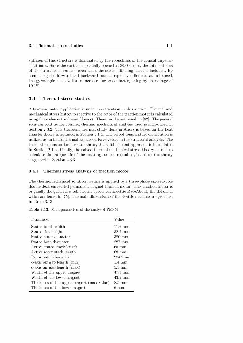
3.4 Thermal stress studies 101
stiffness of this structure is dominated by the robustness of the conical impeller-shaft joint. Since the contact is partially opened at 30,000 rpm, the total stiffnessof the structure is reduced even when the stress-stiffening effect is included. Bycomparing the forward and backward mode frequency difference at full speed,the gyroscopic effect will also increase due to contact opening by an average of10.1%.
3.4 Thermal stress studies
A traction motor application is under investigation in this section. Thermal andmechanical stress history respective to the rotor of the traction motor is calculatedusing finite element software (Ansys). These results are based on [92]. The generalsolution routine for coupled thermal mechanical analysis used is introduced inSection 2.3.2. The transient thermal study done in Ansys is based on the heattransfer theory introduced in Section 2.1.4. The solved temperature distribution isutilized as an initial thermal expansion force vector in the structural analysis. Thethermal expansion force vector theory 3D solid element approach is formulatedin Section 2.1.2. Finally, the solved thermal mechanical stress history is used tocalculate the fatigue life of the rotating structure studied, based on the theorysuggested in Section 2.3.3.
3.4.1 Thermal stress analysis of traction motor
The thermomechanical solution routine is applied to a three-phase sixteen-poledouble-deck embedded permanent magnet traction motor. This traction motor isoriginally designed for a full electric sports car Electric RaceAbout, the details ofwhich are found in [75]. The main dimensions of the electric machine are providedin Table 3.13.
Table 3.13. Main parameters of the analyzed PMSM
Parameter ValueStator tooth width 11.6 mmStator slot height 32.5 mmStator outer diameter 380 mmStator bore diameter 287 mmActive stator stack length 65 mmActive rotor stack length 68 mmRotor outer diameter 284.2 mmd-axis air gap length (min) 1.4 mmq-axis air gap length (max) 5.5 mmWidth of the upper magnet 47.9 mmWidth of the lower magnet 43.9 mmThickness of the upper magnet (max value) 8.5 mmThickness of the lower magnet 6 mm

102 3 Studies of rotating structures
The structure of a single pole of the analyzed PMSM is depicted in Figure 3.33.As presented in [75], the majority of the electric machine losses occur in the statorwindings. In order to obtain proper cooling for the stator, the cooling of thePMSMs is carried out by combining force air cooling in the air gap region andliquid cooling in the stator frame. Most of the Joule and stator iron losses areremoved by liquid cooling, and the rotor surface is cooled by forced air cooling.Because of this, the machine can be regarded as the open type.
Figure 3.33. Structure of one pole of the analyzed PMSM
The input for the thermomechanical analysis consists of the torque and rotationalspeed from the machine drive cycle and the corresponding thermal loads. Allthe input variables are entered as a function of time. In the studied case, themeasured data from the Nürburgring Nordschleife race track according to [75]is used as a drive cycle. The measured rotational speed, torque, voltage andcurrent on the rear left electric motor during one race track lap are presented inFigure 3.34.
The thermal loads within the drive cycle – that is, the iron losses in the rotorlaminations and the eddy current losses in the permanent magnets – were calculatedby 2D FEM. The eddy current losses in the permanent magnets were calculated bytreating them as short-circuited solid conductors in the transient FEA. Rotor ironloss calculation was performed using a loss-surface model, which was implementedin the Flux2D software package by Cedrat. The loss calculation was performed at1000 rpm by applying transient FEM for a whole useful torque region, from zeroto break-down torque. Temperature effects on the electromagnetic performancewere not taken into account. Because eddy current losses are proportional tofrequency squared, the losses at any measured rotational speed and torque pointcan be calculated as based on the previous loss calculation performed at 1000 rpm,using the following relation:
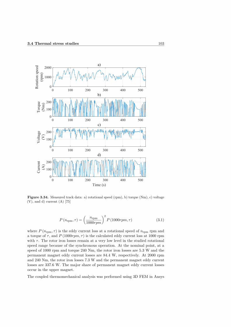
3.4 Thermal stress studies 103
0 100 200 300 400 5000
1000
2000
Rot
atio
n sp
eed
(rpm
)
a)
0 100 200 300 400 5000
100
200
Tor
que
(Nm
)
b)
0 100 200 300 400 5000
100
200
Vol
tage
(V)
c)
0 100 200 300 400 500
Time (s)
0
100
200
Cur
rent
(A)
d)
Figure 3.34. Measured track data: a) rotational speed (rpm), b) torque (Nm), c) voltage(V), and d) current (A) [75]
P (nrpm, τ) =(
nrpm1000rpm
)2P (1000rpm, τ) (3.1)
where P (nrpm, τ) is the eddy current loss at a rotational speed of nrpm rpm anda torque of τ , and P (1000rpm, τ) is the calculated eddy current loss at 1000 rpmwith τ . The rotor iron losses remain at a very low level in the studied rotationalspeed range because of the synchronous operation. At the nominal point, at aspeed of 1000 rpm and torque 240 Nm, the rotor iron losses are 5.3 W and thepermanent magnet eddy current losses are 84.4 W, respectively. At 2000 rpmand 240 Nm, the rotor iron losses 7.3 W and the permanent magnet eddy currentlosses are 337.6 W. The major share of permanent magnet eddy current lossesoccur in the upper magnet.The coupled thermomechanical analysis was performed using 3D FEM in Ansys
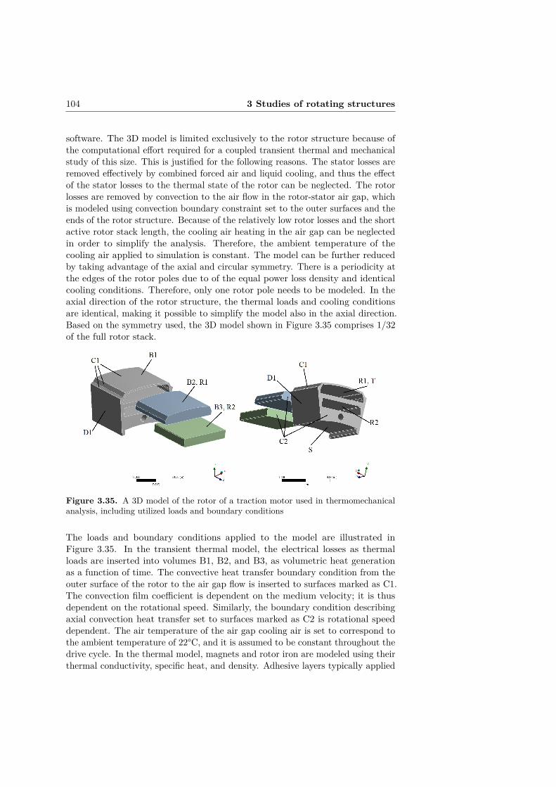
104 3 Studies of rotating structures
software. The 3D model is limited exclusively to the rotor structure because ofthe computational effort required for a coupled transient thermal and mechanicalstudy of this size. This is justified for the following reasons. The stator losses areremoved effectively by combined forced air and liquid cooling, and thus the effectof the stator losses to the thermal state of the rotor can be neglected. The rotorlosses are removed by convection to the air flow in the rotor-stator air gap, whichis modeled using convection boundary constraint set to the outer surfaces and theends of the rotor structure. Because of the relatively low rotor losses and the shortactive rotor stack length, the cooling air heating in the air gap can be neglectedin order to simplify the analysis. Therefore, the ambient temperature of thecooling air applied to simulation is constant. The model can be further reducedby taking advantage of the axial and circular symmetry. There is a periodicity atthe edges of the rotor poles due to of the equal power loss density and identicalcooling conditions. Therefore, only one rotor pole needs to be modeled. In theaxial direction of the rotor structure, the thermal loads and cooling conditionsare identical, making it possible to simplify the model also in the axial direction.Based on the symmetry used, the 3D model shown in Figure 3.35 comprises 1/32of the full rotor stack.
Figure 3.35. A 3D model of the rotor of a traction motor used in thermomechanicalanalysis, including utilized loads and boundary conditions
The loads and boundary conditions applied to the model are illustrated inFigure 3.35. In the transient thermal model, the electrical losses as thermalloads are inserted into volumes B1, B2, and B3, as volumetric heat generationas a function of time. The convective heat transfer boundary condition from theouter surface of the rotor to the air gap flow is inserted to surfaces marked as C1.The convection film coefficient is dependent on the medium velocity; it is thusdependent on the rotational speed. Similarly, the boundary condition describingaxial convection heat transfer set to surfaces marked as C2 is rotational speeddependent. The air temperature of the air gap cooling air is set to correspond tothe ambient temperature of 22°C, and it is assumed to be constant throughout thedrive cycle. In the thermal model, magnets and rotor iron are modeled using theirthermal conductivity, specific heat, and density. Adhesive layers typically applied
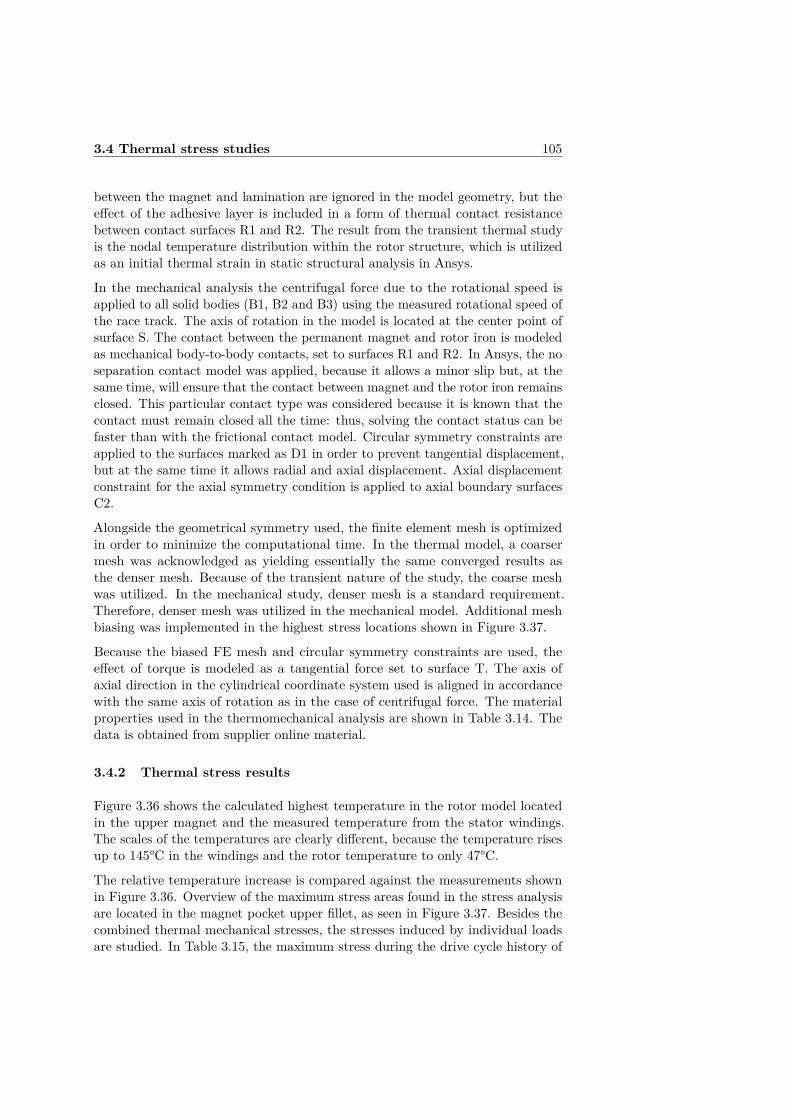
3.4 Thermal stress studies 105
between the magnet and lamination are ignored in the model geometry, but theeffect of the adhesive layer is included in a form of thermal contact resistancebetween contact surfaces R1 and R2. The result from the transient thermal studyis the nodal temperature distribution within the rotor structure, which is utilizedas an initial thermal strain in static structural analysis in Ansys.
In the mechanical analysis the centrifugal force due to the rotational speed isapplied to all solid bodies (B1, B2 and B3) using the measured rotational speed ofthe race track. The axis of rotation in the model is located at the center point ofsurface S. The contact between the permanent magnet and rotor iron is modeledas mechanical body-to-body contacts, set to surfaces R1 and R2. In Ansys, the noseparation contact model was applied, because it allows a minor slip but, at thesame time, will ensure that the contact between magnet and the rotor iron remainsclosed. This particular contact type was considered because it is known that thecontact must remain closed all the time: thus, solving the contact status can befaster than with the frictional contact model. Circular symmetry constraints areapplied to the surfaces marked as D1 in order to prevent tangential displacement,but at the same time it allows radial and axial displacement. Axial displacementconstraint for the axial symmetry condition is applied to axial boundary surfacesC2.
Alongside the geometrical symmetry used, the finite element mesh is optimizedin order to minimize the computational time. In the thermal model, a coarsermesh was acknowledged as yielding essentially the same converged results asthe denser mesh. Because of the transient nature of the study, the coarse meshwas utilized. In the mechanical study, denser mesh is a standard requirement.Therefore, denser mesh was utilized in the mechanical model. Additional meshbiasing was implemented in the highest stress locations shown in Figure 3.37.
Because the biased FE mesh and circular symmetry constraints are used, theeffect of torque is modeled as a tangential force set to surface T. The axis ofaxial direction in the cylindrical coordinate system used is aligned in accordancewith the same axis of rotation as in the case of centrifugal force. The materialproperties used in the thermomechanical analysis are shown in Table 3.14. Thedata is obtained from supplier online material.
3.4.2 Thermal stress results
Figure 3.36 shows the calculated highest temperature in the rotor model locatedin the upper magnet and the measured temperature from the stator windings.The scales of the temperatures are clearly different, because the temperature risesup to 145°C in the windings and the rotor temperature to only 47°C.
The relative temperature increase is compared against the measurements shownin Figure 3.36. Overview of the maximum stress areas found in the stress analysisare located in the magnet pocket upper fillet, as seen in Figure 3.37. Besides thecombined thermal mechanical stresses, the stresses induced by individual loadsare studied. In Table 3.15, the maximum stress during the drive cycle history of

106 3 Studies of rotating structures
Table 3.14. Material parameters of the rotor components
Material property Magnets Steel Adhesive(Neorem753A) (M270-50A)
Density (kg/m3) 7600 7650 1207Young’s modulus (MPa) 150,000 200,000 -Poisson’s ratio 0.24 0.3 -Yield strength (MPa) 75 470 -Ultimate strength (MPa) 290 585 -Specific heat (J/(kg C)) 450 460 1173Thermal expansion (1/K) 6e−6 1.2e−5 -Thermal conductivity (W/(m K)) 8.5 39 0.3
0 100 200 300 400 500
Time (s)
50
100
150
Mea
sure
d te
mpe
ratu
re (
C)
25
35
45
Cal
cula
ted
tem
pera
ture
(C
)
Tmeasured
Tmax
Figure 3.36. Measured stator winding temperature vs. calculated rotor temperature
each loading case studied is presented, along with the corresponding design safetyfactor. The safety factors are calculated against the lamination material yieldstrength shown in Table 3.14.
The maximum von Mises stress caused by mechanical, thermal, and combinedloads during the studied load cycle are presented in Figure 3.38. The curves aresketched with a black dotted line, red dashed line and blue solid line, respectively.The mechanical stress consistently follows the rotational speed of the rotor. Thetangential forces caused by the torque play a minor role, whereas the centrifugalforce is the main contributor to the mechanical stress. During the drive cycle, themaximum mechanical stress does not exceed 43 MPa. The maximum temperaturedifference over the simulated time is presented in Figure 3.39.
For better visualization, the stress and temperature distributions in the FE modelduring the load cycle are presented in Figures 3.40–3.42 at time steps 100 s, 280 s
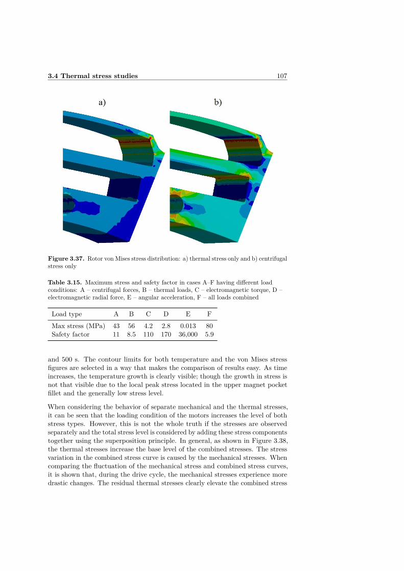
3.4 Thermal stress studies 107
Figure 3.37. Rotor von Mises stress distribution: a) thermal stress only and b) centrifugalstress only
Table 3.15. Maximum stress and safety factor in cases A–F having different loadconditions: A – centrifugal forces, B – thermal loads, C – electromagnetic torque, D –electromagnetic radial force, E – angular acceleration, F – all loads combined
Load type A B C D E FMax stress (MPa) 43 56 4.2 2.8 0.013 80Safety factor 11 8.5 110 170 36,000 5.9
and 500 s. The contour limits for both temperature and the von Mises stressfigures are selected in a way that makes the comparison of results easy. As timeincreases, the temperature growth is clearly visible; though the growth in stress isnot that visible due to the local peak stress located in the upper magnet pocketfillet and the generally low stress level.
When considering the behavior of separate mechanical and the thermal stresses,it can be seen that the loading condition of the motors increases the level of bothstress types. However, this is not the whole truth if the stresses are observedseparately and the total stress level is considered by adding these stress componentstogether using the superposition principle. In general, as shown in Figure 3.38,the thermal stresses increase the base level of the combined stresses. The stressvariation in the combined stress curve is caused by the mechanical stresses. Whencomparing the fluctuation of the mechanical stress and combined stress curves,it is shown that, during the drive cycle, the mechanical stresses experience moredrastic changes. The residual thermal stresses clearly elevate the combined stress

108 3 Studies of rotating structures
0 100 200 300 400 500
Time (s)
0
20
40
60
80
Str
ess
(MP
a)
Mechanical stressThermal stressCombined stress
Figure 3.38. Von Mises stress history in magnet pocket upper fillet with differentloading conditions: pure mechanical load, pure thermal load and combined load
peaks. Thermal and mechanical stresses have different dominating multiaxialstress components. For this reason, within a certain period over the stress history,these stresses combined are actually less than the thermal stresses alone.
According to Figure 3.37, the critical area where the maximum stress occurs isthe uppermost corner. Using Equations (2.123) and (2.124) the equivalent stress∆σeq and the number of cycles Nf are calculated and shown in Table 3.16. Acomparison between the equivalent stresses σeq calculated for the fatigue studyand maximum von Mises stresses in the drive cycle σmax caused by mechanical,thermal and combined loads is illustrated in Figure 3.43. Based on the publishedfatigue test results for a similar rotor laminate material in [31], the followingfatigue strength coefficient, fatigue strength exponent and S-N curve slope for themachine cut edges are adopted in this study: σ′f = 673.25 MPa, be = -0.09559and β = 3.
Table 3.16. Fatigue analysis results of three different load conditions
Stress type Mechanical Thermal Combined∆σeq (MPa) 100 76.4 256Nf (1× 10⁶ cycles) 3.2× 10⁵ 5.5× 10⁶ 17
3.4.3 Discussion
The calculated highest temperature point in the rotor model located in the uppermagnet as well as the measured temperature from the stator windings are shownin Figure 3.36. The trends of the curves can be compared with each other, eventhough the temperatures are obtained from different locations. The calculated

3.4 Thermal stress studies 109
0 50 100 150 200 250 300 350 400 450 500
Time (s)
0
5
10
15
20
Tem
pera
ture
(C
)
∆ TMAX
Figure 3.39. The maximum temperature difference of the FE model during thesimulation
(a) Temperature distribution at 100 s (b) Stress distribution at 100 s
Figure 3.40. Rotor temperature and stress distribution at 100 s
temperature increases rapidly between 70 and 100 s. The temperature in the rotormodel increases more slowly than in the windings after 100 s. After the time pointof 240 s, the rotor temperature starts to increase faster than the temperature inthe windings. At the time point 280 s, the rate of temperature increase becomesslower again, until the final rapid increase directly before the end of the cycle.
The relative temperature increase is compared against the measured temperaturedata in Figure 3.36. Based on the comparison, the faster temperature increasein the rotor is related to driving at full throttle, which can be obtained from therotational speed curve in Figure 3.34. Based on this finding, the temperatureincrease in the rotor lamination is highly dependent on the loading of the motor.The windings are indirectly cooled by liquid cooling. Because of this, thetemperature change in the windings is steadier along the drive cycle than inthe rotor. Based on the general trend of constantly increasing temperature frombeginning till the end of the drive cycle, it appears that the motor has not
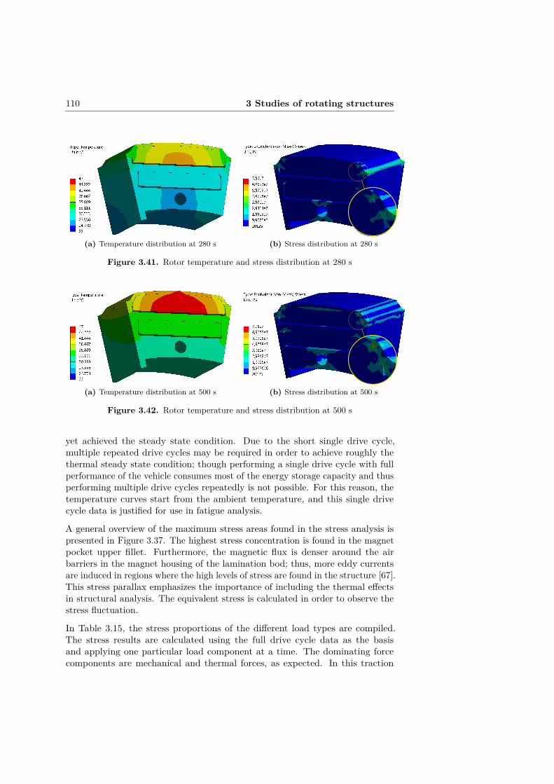
110 3 Studies of rotating structures
(a) Temperature distribution at 280 s (b) Stress distribution at 280 s
Figure 3.41. Rotor temperature and stress distribution at 280 s
(a) Temperature distribution at 500 s (b) Stress distribution at 500 s
Figure 3.42. Rotor temperature and stress distribution at 500 s
yet achieved the steady state condition. Due to the short single drive cycle,multiple repeated drive cycles may be required in order to achieve roughly thethermal steady state condition; though performing a single drive cycle with fullperformance of the vehicle consumes most of the energy storage capacity and thusperforming multiple drive cycles repeatedly is not possible. For this reason, thetemperature curves start from the ambient temperature, and this single drivecycle data is justified for use in fatigue analysis.
A general overview of the maximum stress areas found in the stress analysis ispresented in Figure 3.37. The highest stress concentration is found in the magnetpocket upper fillet. Furthermore, the magnetic flux is denser around the airbarriers in the magnet housing of the lamination bod; thus, more eddy currentsare induced in regions where the high levels of stress are found in the structure [67].This stress parallax emphasizes the importance of including the thermal effectsin structural analysis. The equivalent stress is calculated in order to observe thestress fluctuation.
In Table 3.15, the stress proportions of the different load types are compiled.The stress results are calculated using the full drive cycle data as the basisand applying one particular load component at a time. The dominating forcecomponents are mechanical and thermal forces, as expected. In this traction
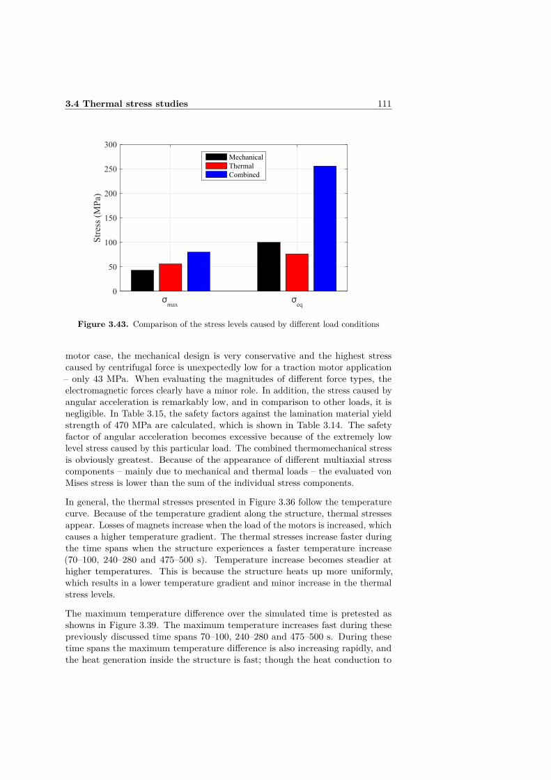
3.4 Thermal stress studies 111
σmax
σeq
0
50
100
150
200
250
300
Str
ess
(MP
a)
MechanicalThermalCombined
Figure 3.43. Comparison of the stress levels caused by different load conditions
motor case, the mechanical design is very conservative and the highest stresscaused by centrifugal force is unexpectedly low for a traction motor application– only 43 MPa. When evaluating the magnitudes of different force types, theelectromagnetic forces clearly have a minor role. In addition, the stress caused byangular acceleration is remarkably low, and in comparison to other loads, it isnegligible. In Table 3.15, the safety factors against the lamination material yieldstrength of 470 MPa are calculated, which is shown in Table 3.14. The safetyfactor of angular acceleration becomes excessive because of the extremely lowlevel stress caused by this particular load. The combined thermomechanical stressis obviously greatest. Because of the appearance of different multiaxial stresscomponents – mainly due to mechanical and thermal loads – the evaluated vonMises stress is lower than the sum of the individual stress components.
In general, the thermal stresses presented in Figure 3.36 follow the temperaturecurve. Because of the temperature gradient along the structure, thermal stressesappear. Losses of magnets increase when the load of the motors is increased, whichcauses a higher temperature gradient. The thermal stresses increase faster duringthe time spans when the structure experiences a faster temperature increase(70–100, 240–280 and 475–500 s). Temperature increase becomes steadier athigher temperatures. This is because the structure heats up more uniformly,which results in a lower temperature gradient and minor increase in the thermalstress levels.
The maximum temperature difference over the simulated time is pretested asshowns in Figure 3.39. The maximum temperature increases fast during thesepreviously discussed time spans 70–100, 240–280 and 475–500 s. During thesetime spans the maximum temperature difference is also increasing rapidly, andthe heat generation inside the structure is fast; though the heat conduction to
112 3 Studies of rotating structures
the outer surface of the structure occurs more slowly. Therefore, when losses areincreased quickly, the temperature difference rises.
Both the thermal stress alone and the combined stress are basically constantlyincreasing, according to Figure 3.38. Even so, Figure 3.39 shows that thetemperature difference at time step 450 s is actually as low as it was at 100 s.This can be explained by slow distribution of the heat in solid bodies due totransient heat conduction. The heat energy is constantly flowing to the structuredue to electrical losses. After some time, the difference between the minimum andmaximum temperature of the structure will decline, due to heat conduction. Inaddition, the forced air cooling in the rotor airgap becomes more efficient whenthe surface temperature is increased.
The equivalent stresses σeq and maximum stresses in the drive cycle σmax causedby mechanical, thermal, and combined loads calculated for the fatigue study areillustrated in Figure 3.43 for comparison purposes. The mechanical stresses werecalculated using the centrifugal force and electromagnetic torque as loads in theFE model, whereas the thermal stresses were calculated using only the initialthermal strain condition as the input load. The combined stresses were calculatedusing all the aforementioned loads in the same model. When the maximum stresspeaks are observed according to Figure 3.43, the thermal stresses are higher thanthe mechanical stresses. The thermal stress levels are lower than the equivalentstress levels of the mechanical stresses because the fluctuation of mechanicalstresses is much more aggressive, due to the rapidly and constantly changingrotational speed. The results show a considerably high equivalent stress level,when the rapidly changing mechanical stresses and relatively high though slowlychanging thermal stresses are combined. Based on these results, it is importantto take both the mechanical and thermal loads into account. In addition, thelifetime calculation becomes important, when the loads are highly cyclic andloading conditions are constantly changing.

Chapter 4Conclusions
Comprehensive theory of both 3D solid element based structural and heat transferfinite element modeling is given, with a number of solution routines for variousanalyses of rotating structures. This work contains an extensive set of results ofrotating structures made using both the beam and 3D solid element-based finiteelement methods. The beam element approach is utilized to study the rotor andbearing stress history during the rotor dropdown event. The 3D solid elementapproach is used for studying rotors having multiple parts, thus having contacts,and the contact-based nonlinear behavior under centrifugal load. In addition,thermal mechanical stress history of a rotor in the traction motor and the fatiguelife results are presented and discussed in detail. Custom programmed 3D solidfinite elements and solution routines, including a proposed contact detection andconstraint equation methods in the 3D domain, are utilized in order to generatethe presented results. In addition, commercial finite element software Ansys isused for coupled thermal mechanical stress study. Experimental results are usedas basis for all the numerical studies of rotating structures presented.
4.1 Summary of solution methods
Multiple solution methods developed for studying various rotating machineryaspect are presented and utilized. A discussion of benefits and limitations ofdifferent constraint equation methods is presented. The custom, applicationspecific, developed trial force constraint method is presented and tested extensively.In addition, the constraint error aspects are studied and discussed using this customdevelop trial force method against the augmented Lagrangian method commonlyused in commercial FE software. For proof, an exact method, multipoint constraintmethod, is applied and benefits and limitations of using this particular methodare discussed.Aspects of obtaining the solution are also discussed. Constraint equation methodsthat do not require the cross coupling description in the stiffness matrix canbe distributed and solved separately. This becomes handy if the problem size
113

114 4 Conclusions
exceeds the computational memory limitations. When utilizing the 3D solid finiteelement approach, the use of DOF reduction methods may become necessary.Thus, the 3D solid element based models can be reduced by applying, for example,the modal reduction method, which is commonly used also with beam elements.This method is relatively easy to use and very practical for transient and modalproblems. Although, this method can typically yield error, if it is applied forsolving contact problems, or in general static structural problems. For staticproblems, a static condensation, also known as Guyan reduction, can be applied.
4.2 Rotor dropdown studies
The sudden contact of active magnetic bearings supported rotor during dropdownevent was studied. The study introduces the rotor stress behavior during dropdownand the effect of backup bearing misalignment to the rotor dropdown behavior.The backup bearing alignment is a relevant issue for designing the rotor-bearingsystem. The rotor transient response was studied using the finite element methodand the problem was simplified by using modal reduction method for computationalreasons. The first moments after the beginning of the dropdown event is typicallythe most chaotic, thus it was considered that simulation time of 0.5 seconds islong enough to reveal the dynamic performance of the rotor. The measurementresults of the experimental modal analysis performed to physical rotor were usedfor fine-tuning the rotor FE model. Three different horizontal alignment caseswere studied. The results observed were the orbits of during rotor-bearing contactand the bending and shear stresses of the rotor during the dropdown event.Based on the rotor orbit and stress results the backup bearing misalignment hasa great effect on the dynamic behavior of the rotor. When no misalignment wasintroduced, the rotor orbits are smooth and the rotor settles in a short period onthe bottom of the bearing inner ring. Rotor oscillation increases as introducedbearing misalignment increases. Even when the maximum bearing misalignmentwas introduced the rotor did not get into the whirling motion.The introduced bearing misalignment has an impact the rotor bending stressresults. When additional misalignment is introduced, the rotor stresses areincreasing in the gravitational direction. The misalignment of backup bearingsin horizontal direction yields also proportionally increased bending stress incorresponding direction. In general, the increase of shear stress in directionnormal to gravitational force is nominal, although the impact is more observablein horizontal direction (in perpendicular direction to gravitational force).This study shows that the backup bearing misalignment has a great effect onthe dynamic behavior and the rotor motions after a dropdown. The rotor orbitsindicate that critical whirling of the rotor could occur if the contacting surfaces arecontaminated or otherwise are having some roughness that can induce a greatercontact friction, or the damping properties designed properly. The direction ofmisalignment with respect to the direction of misalignment could be studied inthe future. In addition, the behavior of physical rotor during dropdown eventshould be measured using the position sensors.
4.3 Bearing stress studies 115
4.3 Bearing stress studies
The stresses in a backup bearing during dropdown of an AMB-supported rotorwere modeled using a numerical simulation. In this study, the system investigatedcompromised of a flexible rotor, two AMBs and backup bearings. The deepgroove ball bearing were modeled as backup bearings using a simplified ballbearing model. The flexible rotor was modeled using Timoshenko finite beamelements. The Hertzian contact stresses in the backup bearing were evaluatedin this study. The contact stresses in the backup bearing are influenced by thematerial properties used in backup bearing as well as the dynamic behavior ofrotor. The stress history of the backup bearing based on the transient forceequilibrium was calculated. The results showed that the normal contact forcesinside the bearing are not evenly distributed among all the balls of the backupbearing. During the first contact, the balls that are initially located in the loadedzone of the backup bearing experience higher stress. The stress experienced byindividual ball in the loaded zone is dependent on the ball position, which willchange during the rotor dropdown by means of the friction forces induced byrotor-bearing contact.
4.4 Summary of internal contact studies
A custom internal contact model is developed and utilized for studying contactbehavior at high-speed operation. The results are presented and compared to theresults generated by using commercial software (Ansys). In addition, the inclusionof the stress-stiffening effect is also studied extensively. Two example cases arestudied; an experimentally verified test shaft assembly with shrink fit interferencejoint and a conical impeller assembly. With the test shaft assembly, a number ofdifferent radial interferences were studied and compared to the measured data.Based on the results, it was noticed that the amount of radial interference in theshrink-fitted joint will not in fact change the free-free natural bending frequenciesof the assembly noticeably when the initial stress state is relatively low.The partial contact opening with the conical impeller assembly was studied anddetected using a custom frictionless contact model. The same conditions werestudied also using Ansys software for comparison purposes. The custom developedcontact model will update the contact status on every speed step. The resultsgenerated using this custom contact detection model differ moderately from theones solved using Ansys. It seems the contact status is not updated in Ansysby default during the regular solution of damped eigenvalue problem, when therotational speed is used as a variable for a step solution for generating Campbelldiagram. Based on the presented results, the stress-stiffening effect should beincluded into eigenvalue calculation particularly in cases, where relatively heavybodies attached on the shaft using interference fittings are rotating at high-speeds.In addition, the contact region constraint error was studied in detail. Twocomparison cases with both custom code and Ansys were studied. The MPCmethod with frictionless contact was determined to be more accurate than the
116 4 Conclusions
developed trial force method that is based on used stiffness coefficients havingsimilarities to penalty function method. On Ansys side, normal Lagrangianmethod was determined to be more accurate than the augmented Lagrangianmethod in this particular test case. Ansys seems to use a significantly highernumber of iterations when solving contact problems, compared to the customcode method.
4.5 Thermal stress studies
A solution method for calculating the combined thermal mechanical stress usingloading history and fatigue life analysis of a traction motor is presented. A finiteelement method was utilized to solve coupled field thermal and mechanical problemusing commercial FE software. Based on the results, a significant change betweenmechanical and combined thermomechanical stress levels was observed. In addition,the predicted fatigue life is highly dependent on whether the thermal loads aretaken into account or not. The total stress levels of the studied traction motorwere acceptable due to the conservative approach adopted in the design process,even when the thermal effects were included. By sacrificing the electromagneticperformance, the mechanical durability of the rotor can be increased. Based on theresults presented, a comprehensive thermomechanical stress analysis is essentialfor optimal design. The results were obtained by utilizing the thermomechanicalcoupled field solution routine presented in this work. This solution routine couldbe extended for a electro–thermomechanical coupled problem of interior PMSMs.
4.6 Future work
Writing this dissertation has raised multiple interesting future research topics.Starting from beam element modeling, the modeling of the AMB levitation and therotor translational inertial state due to this levitation while the rotor dropdownis initiated should be studied, and the effect of this initial condition – the AMBlevitation – should be investigated.
The inclusion of the flexible frame structure of the electric motor and the stiffnessand damping of the foundation to eigenvalue analysis could yield more realisticresults. In the rotor-frame system, the mass of the frame contributes to the rotoreigenfrequencies and vice versa. Transient simulation should be implementedfor including possible contact-induced nonlinearities, such as directional depen-dent stiffness and damping in bolt-jointed frame leg-foundation connections, forexample.
The proposed direct node-to-node contact modeling method developed for eigen-value problems of 3D solid element modeled rotors would need to be updated toinclude the frictional contact forces and contact slippage detection for transientsimulation needs. In addition, the thermal expansion-induced geometric changeswould require an extension from node-to-node contact detection to node-to-nodegroup detection, in order to properly include geometric changes and contact

4.6 Future work 117
slippage. The thermal expansion forces could be included in an analysis ofhigh-speed gas turbine components using proposed node-to-node group contactdetection. In addition, the fatigue life of the components of high-speed gas turbinecould be studied. Inclusion of thermal effects with the proposed solution routinefor the Campbell diagram for a rotor having multiple parts would require a modelupdate during the process. As temperature changes, thermally non-linear materialproperties such as the thermal expansion coefficient, elastic modulus, thermalconductivity and specific heat coefficient should be updated. Because of this, amodel update routine should be developed.
Investigation of various DOF reduction methods could be useful for 3D solidelement based rotor dynamics simulations. For transient or eigenvalue problems,the use of dynamically condensed superelements could be useful, since this methodcan be applied for rotors having contacts, the contact treatment can be doneefficiently, and there is no need for coordinate mapping – unlike using modalreduction, since the master DOFs selected are described using physical coordinates.In addition, superelements can be utilized for transient beam element based rotor-bearing contact problems.

118 4 Conclusions

Bibliography
[1] Abawi, A. T. The Bending of Bonded Layers Due to Thermal Stress.Hughes Research Laboratories (2004), 1–11.
[2] Adeeb, S. Introduction to Solid Mechanics and Finite Element Analysisusing Mathematica. Kendall Hunt, 2011.
[3] Adhikari, S. Damping Modelling using Generalized Proportional Damping.Journal of Sound and Vibration 293 (2006), 156–170.
[4] ANSYS, Inc. ANSYS Mechanical APDL Theory Reference. ANSYS, Inc.,2013.
[5] Boldea, I., Tutelea, L. N., Parsa, L., and Dorrell, D. AutomotiveElectric Propulsion Systems with Reduced or no Permanent Magnets: Anoverview. IEEE Transactions on Industrial Electronics 61, 10 (2014), 5696–5711.
[6] Bracikowski, N., Hecquet, M., Brochet, P., and Shirinskii, S. V.Multiphysics Modeling of a Permanent Magnet Synchronous Machine byusing Lumped Models. IEEE Transactions on Industrial Electronics 59, 6(2012), 2426–2437.
[7] Çallioğlu, H., Sayer, M., and Demir, E. Stress Analysis of FunctionallyGraded Discs under Mechanical and Thermal Loads. Indian Journal ofEngineering and Materials Sciences 18, 2 (2011), 111–118.
[8] Campbell, F. C. Elements of Metallurgy and Engineering Alloys. ASMInternational, 2008.
[9] Cao, J., Allaire, P., Dimond, T., van Rensburg, J. J. J., and Klatt,C. Rotor Drop Analyses and Auxiliary Bearing System Optimization forAMB Supported Rotor/Experimental Validation – Part I: Analysis Method.The 15th International Symposium on Magnetic Bearings (2016).
[10] Cao, J., Allaire, P., Dimond, T., van Rensburg, J. J. J., and Klatt,C. Rotor Drop Analyses and Auxiliary Bearing System Optimization forAMB Supported Rotor/Experimental Validation – Part II: Experiment andOptimization. The 15th International Symposium on Magnetic Bearings(2016).
119
120 BIBLIOGRAPHY
[11] Celebi, K., Yarimpabuc, D., and Keles, I. A Novel Approach toThermal and Mechanical Stresses in a FGM Cylinder with Exponentially-Varying Properties. Journal of Theoretical and Applied Mechanics 55, 1(2017), 343–351.
[12] Chai, F., Li, Y., Liang, P., and Pei, Y. Calculation of the maximummechanical stress on the rotor of interior permanent-magnet synchronousmotors. IEEE Transactions on Industrial Electronics 63, 6 (2016), 3420–3432.
[13] Chen, S.-Y. An Equivalent Direct Modeling of a Rotary Shaft with Hot-FitComponents using Contact Element Modal Analysis Results. Computersand Mathematics with Applications 64, 5 (2012), 1093–1099.
[14] Chen, S.-Y., Kung, C., and Hsu, J.-C. Dynamic Analysis of a RotaryHollow Shaft with Hot-Fit Part using Contact Elements with Friction.Transactions of the Canadian Society for Mechanical Engineering 35, 3(2011), 461–474.
[15] Chen, S.-Y., Kung, C., Liao, T.-T., and Chen, Y.-H. DynamicEffects of the Interference Fit of Motor Rotor on the Stiffness of a HighSpeed Rotating Shaft. Transactions of the Canadian Society for MechanicalEngineering 34, 2 (2010), 243–261.
[16] Chen, W. J., and Gunter, E. J. Introduction to Dynamics of Rotor-Bearing Systems. Trafford Publishing, 2005.
[17] Chen, W. T., and Nelson, C. W. Thermal Stress in Bonded Joints.IBM Journal of Research and Development 23, 2 (1979), 179–188.
[18] Climente-Alarcon, V., Antonino-Daviu, J. A., Strangas, E. G.,and Riera-Guasp, M. Rotor–Bar Breakage Mechanism and Prognosisin an Induction Motor. IEEE Transactions on Industrial Electronics 62, 3(2015), 1814–1825.
[19] Cole, M. O. T., Keogh, P. S., and Burrows, C. R. The DynamicBehavior of a Rolling Element Auxiliary Bearing Following Rotor Impact.Journal of Tribology 124, 2 (2002), 406–413.
[20] Cook, R. D. Concept and Application of Finite Element Analysis. JohnWiley & Sons, 1988.
[21] Dajaku, G., Hofmann, H., Hetemi, F., Dajaku, X., Xie, W., andGerling, D. Comparison of Two Different IPM Traction Machines withConcentrated Winding. IEEE Transactions on Industrial Electronics 63, 7(2016), 4137–4149.
[22] de Santiago, J., Bernhoff, H., Ekergård, B., Eriksson, S.,Ferhatovic, S., Waters, R., and Leijon, M. Electrical Motor Drivelinesin Commercial All-Electric Vehicles: A review. IEEE Transactions onVehicular Technology 61, 2 (2012), 475–484.
BIBLIOGRAPHY 121
[23] Donadon, M. V., Bringhenti, C., and Menezes, J. C. The StressStiffening Effects on the Natural Frequecies of Gas Turbine Blades. VINational Congress of Mechanical Engineering (2010).
[24] Duda, P. Finite Element Method Formulation in Polar Coordinates forTransient Heat Conduction Problems. Journal of Thermal Science 25, 2(2016), 188–194.
[25] El-Refaie, A. M. Motors/Generators for Traction/PropulsionApplications: A review. IEEE Vehicular Technology Magazine 8, 1 (2013),90–99.
[26] Fatemi, A., Demerdash, N. A. O., Nehl, T. W., and Ionel, D. M.Large-Scale Design Optimization of PM Machines over a Target OperatingCycle. IEEE Transactions on Industry Applications 52, 5 (2016), 3772–3782.
[27] Fatemi, A., and Yang, L. Cumulative Fatigue Damage and Life PredictionTheories: A Survey of the State of the Art for Homogeneous Materials.International Journal of Fatigue 20, 1 (1998), 9–34.
[28] Felippa, C. A. Introduction to Aerospace Structures (ASEN 3112).University of Colorado at Boulder, 2016.
[29] Felippa, C. A. Introduction to Finite Element Methods (ASEN 5007).University of Colorado at Boulder, 2017.
[30] Gabrielson, T. B. Mechanical-Thermal Noise in Micromachined Acousticand Vibration Sensors. IEEE Transactions on Electron Devices 40, 5 (1993),903–909.
[31] Gao, Y., Long, R., Pang, Y., and Lindenmo, M. Fatigue Properties ofan Electrical Steel and Design of EV/HEV IPM Motor Rotors for Durabilityand Efficiency. SAE 2010 World Congress & Exhibition (2010).
[32] Genta, G., Feng, C., and Tonoli, A. Dynamics Behavior of RotatingBladed Discs: A Finite Element Formulation for the Study of Second andHigher Order Harmonics. Journal of Sound and Vibration 329, 25 (2010),5289–5306.
[33] Genta, G., and Silvagni, M. Three-dimensional FEM rotordynamicsand the so-called centrifugal softening of rotors. Memorie Della AccademiaDelle Scienze Di Torino 36 (2012), 3–25.
[34] Genta, G., and Silvagni, M. On Centrifugal Softening in Finite ElementMethod Rotordynamics. Journal of Applied Mechanics 81, 1 (2013), 011001.
[35] Geradin, M., and Kill, N. A New Approach to Finite Element Modellingof Flexible Rotors. Engineering Computations 1 (1984), 52–64.

122 BIBLIOGRAPHY
[36] Halminen, O., Kärkkäinen, A., Sopanen, J., and Mikkola, A.Active Magnetic Bearing-Supported Rotor with Misaligned Cageless BackupBearings: A Dropdown Event Simulation Model. Mechanical Systems andSignal Processing 50–51 (2015), 692–705.
[37] Hobbacher, A. Recommendations for Fatigue Design of Welded Jointsand Components. Springer, 2009.
[38] Inman, D. J. Engineering Vibration. Pearson, 2014.
[39] International Organization for Standardization. ISO1940-1 –Mechanical Vibration – Balance Quality Requirements for Rotors in aConstant (Rigid) State – Part 1: Specification and Verification of BalanceTolerances.
[40] Ishii, T., and Kirk, R. G. Transient Response Technique Applied toActive Magnetic Bearing Machinery During Rotor Drop. Journal of Vibrationand Acoustics-Transactions of the Asme 118, 4 (1999), 154–163.
[41] Jafri, S. M. M. Shrink Fit Effects on Rotordynamic Stability: Experimentaland Theoretical Study. Ph.D. thesis. Texas A&M University, 2007.
[42] Jalali, M. H., Ghayour, M., Ziaei-Rad, S., and Shahriari, B.Dynamic Analysis of a High Speed Rotor-Bearing System. Measurement 53(2014), 1–9.
[43] Jammi, S. R. Rotor Dynamics in Design of a High Speed CryogenicPump for Geo Stationary Launch Vehicles. ASME 2014 InternationalDesign Engineering Technical Conferences and Computers and Informationin Engineering Conference 8 (2014), V008T11A065.
[44] Jia, Z., Peng, X., Guan, Z., Wang, L., and Yue, B. Evaluation of theDegradation of Generator Stator Ground Wall Insulation under MultistressesAging. IEEE Transactions on Energy Conversion 23, 2 (2008), 474–483.
[45] Jiang, T., Ryu, S.-K., Zhao, Q., Im, J., Huang, R., and Ho, P. S.Measurement and Analysis of Thermal Stresses in 3D Integrated StructuresContaining Through-Silicon-Vias. Microelectronics Reliability 53, 1 (2013),53–62.
[46] Kattan, P. I. MATLAB Guide to Finite Elements. Springer, 2008.
[47] Kim, J., Yoon, J.-C., and Kang, B.-S. Finite Element Analysis andModeling of Structure with Bolted Joints. Applied Mathematical Modelling31, 5 (2007), 895–911.
[48] Kirchgäßner, B. Finite Elements in Rotordynamics. ProcediaEngineering 144 (2016), 736–750.

BIBLIOGRAPHY 123
[49] Knetsch, D., Funk, M., Kennerknecht, T., and Eberl, C. LoadData Calculation in Electric Axle Drives and Fatigue Assessment for theElectric Motor Subsystem. Materials Testing 56, 7–8 (2014), 535–541.
[50] Kärkkäinen, A. Dynamic Simulations of Rotors During Drop on RetainerBearings. Ph.D. thesis. Lappeenranta University of Technology, 2007.
[51] Kärkkäinen, A., Sopanen, J., and Mikkola, A. Dynamic Simulationof a Flexible Rotor During Drop on Retainer Bearings. Journal of Soundand Vibration 306, 3–6 (2007), 601–617.
[52] Kulkarni, A., Ranjha, S. A., and Kapoor, A. Fatigue Analysis of aSuspension for an In-Wheel Electric Vehicle. Engineering Failure Analysis68 (2016), 150–158.
[53] Kumar, S., Rao, R., and Rajeevalochanam, B. A. Current Practicesin Structural Analysis and Testing of Aero-Engine Main Shafts. ProcediaEngineering 55 (2007), 499–509.
[54] Kupnik, M., Wygant, I. O., and Khuri-Yakub, B. T. Finite ElementAnalysis of Stress Stiffening Effects in CMUTs. 2008 IEEE InternationalUltrasonics Symposium Proceedings (2008).
[55] Lee, J. G., and Palazzolo, A. Catcher Bearing Life Prediction using aRainflow Counting Approach. Journal of Tribology 134, 3 (2012), 031101.
[56] Lee, Y. L. Fatigue Testing and Analysis: Theory and Practice. Butterworth–Heinemann, 2005.
[57] Lin, Z.-C., and Lee, B.-Y. An investigation of the residual stress ofa machined workpiece considering tool flank wear. Journal of MaterialsProcessing Technology 51, 1–4 (1995), 1–24.
[58] Lindh, P., Gerami Tehrani, M., Lindh, T., Montonen, J. H.,Pyrhönen, J., Sopanen, J. T., Niemelä, M., Alexandrova,Y., Immonen, P., Aarniovuori, L., and Polikarpova, M.Multidisciplinary design of a permanent-magnet traction motor for a hybridbus taking the load cycle into account. IEEE Transactions on IndustrialElectronics 63, 6 (2016), 3397–3408.
[59] Lindh, P. M., Immonen, P., Alexandrova, Y., Gerami Tehrani, M.,Pyrhönen, J. J., and Sopanen, J. T. The Design of Rotor Geometry ina Permanent Magnet Traction Motor for a Hybrid Bus. 2014 InternationalConference on Electrical Machines (ICEM) (2014), 310–315.
[60] Liu, G. R., and Quek, S. S. The Finite Element Method. Butterworth–Heinemann, 2013.
[61] Logan, D. L. A First Course in the Finite Element Method. CengageLearning, 2007.
124 BIBLIOGRAPHY
[62] Logie, W. R., Pye, J. D., and Coventry, J. Thermal Elastic Stressin Sodium Receiver Tubes. Asia Pacific Solar Research Conference (2016),1–12.
[63] Long, S. G., and Zhou, Y. C. Thermal Fatigue of Particle ReinforcedMetal-Matrix Composite Induced by Laser Heating and Mechanical Load.Composites Science and Technology 65, 9 (2005), 1391–1400.
[64] Lu, K. H., Ryu, S.-K., Zhao, Q., Hummler, K., Im, J., Huang, R.,and Ho, P. S. Temperature-dependent Thermal Stress Determinationfor Through-Silicon-Vias (TSVs) by Combining Bending Beam Techniquewith Finite Element Analysis. 2011 Electronic Components and TechnologyConference (2011), 1475–1480.
[65] Lu, K. H., Zhang, X., Ryu, S., Huang, R., and Ho, P. S. ThermalStresses Analysis of 3-D Interconnect. AIP Conference Proceedings 1143,224 (2009), 224–230.
[66] Ma, L. S., and Wang, T. J. Nonlinear Bending and Post-Bucklingof a Functionally Graded Circular Plate under Mechanical and ThermalLoadings. International Journal of Solids and Structures 40, 13–14 (2003),3311–3330.
[67] McFarland, J. D., and Jahns, T. M. Investigation of the RotorDemagnetization Characteristics of Interior PM Synchronous MachinesDuring Fault Conditions. IEEE Transactions on Industry Applications 50,4 (2014), 2768–2775.
[68] Miao, H., Zang, C., and Friswell, M. Model Updating and Validationof a Dual-Rotor System. ISMA2014 International Conference on Noise andVibration Engineering (2014), 2723–2737.
[69] Nandi, A., and Neogy, S. Modelling of Rotors with Three-DimensionalSolid Finite Elements. Journal of Strain Analysis for Engineering Design36, 4 (2001), 359–371.
[70] Neisi, N., Heikkinen, J. E., Sikanen, E., and Sopanen, J. StressAnalysis of a Touchdown Bearing Having an Artificial Crack. ASME 2017International Design Engineering Technical Conferences and Computersand Information in Engineering Conference 8 (2017), V008T12A034.
[71] Neisi, N., Sikanen, E., Heikkinen, J. E., and Sopanen, J. Effectof Off-Sized Balls on Contact Stresses in a Touchdown Bearing. TribologyInternational 120 (2018), 340–349.
[72] Nejati, M., Paluszny, A., and Zimmerman, R. W. A Finite ElementFramework for Modeling Internal Frictional Contact in Three-DimensionalFractured Media using Unstructured Tetrahedral Meshes. Computer Methodsin Applied Mechanics and Engineering 306 (2010), 123–150.
BIBLIOGRAPHY 125
[73] Nelson, H. D. A Finite Rotating Shaft Element using Timoshenko BeamTheory. Journal of Mechanical Design 102, 4 (1980), 793–803.
[74] Nelson, H. D., and McVaugh, J. M. The Dynamics of Rotor-BearingSystems using Finite Elements. Journal of Engineering for Industry 98, 2(1976), 593–600.
[75] Nerg, J., Rilla, M., Ruuskanen, V., Pyrhönen, J., andRuotsalainen, S. Direct-Driven Interior Magnet Permanent-MagnetSynchronous Motors for a Full Electric Sports Car. IEEE Transactions onIndustrial Electronics 61, 8 (2014), 4286–4294.
[76] Nikishkov, G. P. Programming Finite Elements in Java. Springer, 2010.
[77] Paramonov, V. V., and Gonin, I. V. 3D Thermal Stress Analysis forthe CDS Structures. Proceedings of EPAC 2000 (2000), 1990–1992.
[78] Prakash, S., and Puri, V. K. Foundations for Vibrating Machines.Journal of Structural Engineering (Madras) (2006), 1–39.
[79] Qin, Z.-Y., Han, Q.-K., and Chu, F.-L. Analytical Model of BoltedDisk–Drum Joints and its Application to Dynamic Analysis of Jointed Rotor.Proceedings of the Institution of Mechanical Engineers, Part C: Journal ofMechanical Engineering Science 228, 4 (2014), 646–663.
[80] Rao, J. S. Finite Element Methods for Rotor Dynamics. History ofRotating Machinery Dynamics (2011), 269–297.
[81] Rao, J. S. Transient Forward and Backward Whirl of Beam and SolidRotors With Stiffening and Softening Effects. ASME 2011 InternationalDesign Engineering Technical Conferences and Computers and Informationin Engineering Conference 1 (2011), 911–920.
[82] Rao, J. S., and Sreenivas, R. Dynamics of Asymmetric Rotors usingSolid Models. Proceedings of the International Gas Turbine Congress 2003(2003), 1–6.
[83] Rashid, A., and Strömberg, N. An Efficient Sequential Approach forSimulation of Thermal Stresses in Disc Brakes. 15th Nordic Symposium onTribology, NORDTRIB 1 (2012).
[84] Richardson, I.-J., and Hyde, T.-M .and Taylor, J.-W. A Three-Dimensional Finite Element Investigation of the Bolt Stresses in an Aero-Engine Curvic Coupling under a Blade Release Condition. Proceedingsof the Institution of Mechanical Engineers, Part G: Journal of AerospaceEngineering 214, 4 (2000), 231–245.
[85] Saari, J. Thermal Analysis of High-Speed Induction Machines. Ph.D.thesis. Helsinki University of Technology, 1998.
126 BIBLIOGRAPHY
[86] Santos, H. L. V., Luersen, M. A., and Bavastri, C. A. ExperimentalEvaluation of Numerical Models to Represent the Stiffness of LaminatedRotor Cores in Electrical Machines. Engineering Science and Technology,an International Journal 8, 4 (2013), 457–471.
[87] Sasek, J. Eigenfrequency Sensitivity Analysis of Flexible Rotors. Appliedand Computational Mechanics 1, 1 (2012), 289–298.
[88] Schmied, J., and Pradetto, J. C. Behavior of a One Ton Rotor BeingDropped into Auxiliary Bearings. Proceedings of the 3rd InternationalSymposium on Magnetic Bearings (1992), 145–156.
[89] Shimazaki, H., and Shinomoto, S. A Method for Selecting the Bin Sizeof a Time Histogram. Neural Computation 19, 6 (2007), 1503–1527.
[90] Sikanen, E., Halminen, O., Heikkinen, J. E., Sopanen, J., Mikkola,A., and Matikainen, M. Stresses of an AMB-Supported Rotor Arisingfrom the Sudden Contact with Backup Bearings. Proceedings of theASME 2015 International Mechanical Engineering Congress and ExpositionIMECE2015 (2015), V04AT04A039.
[91] Sikanen, E., Heikkinen, J. E., and Sopanen, J. Shrink-FittedJoint Behavior using Three-Dimensional Solid Finite Elements in RotorDynamics with Inclusion of Stress-Stiffening Effect. Advances in MechanicalEngineering 10, 6 (2018), 1–13.
[92] Sikanen, E., Nerg, J., Heikkinen, J. E., Gerami Tehrani, M.,and Sopanen, J. Fatigue Life Calculation Procedure for the Rotor of anEmbedded Magnet Traction Motor Taking into Account ThermomechanicalLoads. Mechanical Systems and Signal Processing 111 (2018), 36–46.
[93] Stimac, G., Braut, S., Bulic, N., and Zigulic, R. Modeling andExperimental Verification of a Flexible Rotor/AMB System. COMPEL –The International Journal for Computation and Mathematics in Electricaland Electronic Engineering 32, 4 (2013), 1244–1254.
[94] Sun, G. Auxiliary Bearing Life Prediction using Hertzian Contact BearingModel. Journal of Vibration and Acoustics 128, 2 (2006), 203–209.
[95] Tannous, M., Cartraud, P., Dureisseix, D., and Torkhani, M. ABeam to 3D Model Switch for Rotor Dynamics Applications. EngineeringStructures 84 (2015), 54–66.
[96] Wagner, M. B., Younan, A., Allaire, P., and Cogill, R. ModelReduction Methods for Rotor Dynamic Analysis: A Survey and Review.International Journal of Rotating Machinery 2010 (2010), 1–17.
[97] Zeng, S. Motion of AMB Rotor in Backup Bearings. Journal of Vibrationand Acoustics 124, 3 (2002), 460–464.

BIBLIOGRAPHY 127
[98] Zhang, J., and Wang, Q. A Finite Element Method for Solving 2DContact Problems with Coulomb Friction and Bilateral Constraints. Journalof Computational Physics (2014) (2014).
[99] Zhao, S., Hilmas, G. E., and Dharani, L. R. Behavior of a CompositeMultidisk Clutch Subjected to Mechanical and Frictionally Excited ThermalLoad. Wear 264, 11–12 (2008), 1059–1068.
[100] Zhou, C. L., Friswell, M. I., and Li, J. Y. Condition Monitoringof Cracked Shaft using Active Magnetic Bearings. Challenges of PowerEngineering and Environment 1 (2007), 494–504.
[101] Zhou, S.-T., and Li, H.-G. Three Dimensional Finite Element Simulationof Solid Rotor System Based on INTESIM and ARPACK Tools. Journal ofSystem Simulation 26, 6 (2014), 1391–1399.
[102] Zienkiewicz, O. C., and Taylor, R. E. The Finite Element Method.McGraw-Hill, 1993.
[103] Zienkiewicz, O. C., and Taylor, R. L. The Finite Element Method:Volume 1 The Basis. Butterworth–Heinemann, 2010.
[104] Zienkiewicz, O. C., and Taylor, R. L. The Finite Element Method:Volume 2 Solid Mechanics. Butterworth–Heinemann, 2010.
[105] Öztürk, T., and Öztürk, Z. Vibration Absorption and Isolationin Dynamically Loaded Foundations. The 14th World Conference onEarthquake Engineering (2008).

128 BIBLIOGRAPHY

Appendix AConstructing element shape functions
In this appendix, a general description of forming isoparametric element shapefunctions, is given. The selection of monomials used for a particular elementwill determine the basic behavior of the element. A good selection of monomialswill guarantee correct and chronologically increasing eigenmodes for the element.Monomials should be selected in chronological order. The number of monomialsselected and the highest order of monomials will increase the number of eigenmodesof the element. Due to the fact the moment matrix P is a square matrix, thenumber of monomials is equal to the number of nodes in the element. Therefore,the greater the number of nodes is in the element, the greater the number ofpossible eigenmodes [60].
Even though the topic is on isoparametric element shape functions, for convenience,the physical coordinates are used to express individual monomials. The vector ofmonomials in three dimensional domain using physical coordinates can be writtenas follows:
pT (x) =[1 x y z xy yz zx x2 y2 z2 · · · xp yp zp
](A.1)
Figures A.1 and A.2 visualize how to generate the monomials in two and threedimensional cases. The moment matrix is formed by placing node coordinatesinto the monomial vector of corresponding node as follows:
P =
pT (x1)pT (x2)
...pT (xn)
(A.2)
By placing the node coordinates into moment matrix we get
129
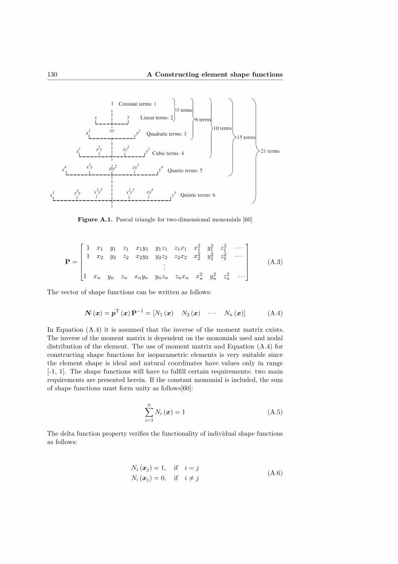
130 A Constructing element shape functions
Figure A.1. Pascal triangle for two-dimensional monomials [60]
P =
1 x1 y1 z1 x1y1 y1z1 z1x1 x2
1 y21 z2
1 · · ·1 x2 y2 z2 x2y2 y2z2 z2x2 x2
2 y22 z2
2 · · ·...
1 xn yn zn xnyn ynzn znxn x2n y2
n z2n · · ·
(A.3)
The vector of shape functions can be written as follows:
N (x) = pT (x) P−1 = [N1 (x) N2 (x) · · · Nn (x)] (A.4)
In Equation (A.4) it is assumed that the inverse of the moment matrix exists.The inverse of the moment matrix is dependent on the monomials used and nodaldistribution of the element. The use of moment matrix and Equation (A.4) forconstructing shape functions for isoparametric elements is very suitable sincethe element shape is ideal and natural coordinates have values only in range[-1, 1]. The shape functions will have to fulfill certain requirements: two mainrequirements are presented herein. If the constant monomial is included, the sumof shape functions must form unity as follows[60]:
n∑i=1
Ni (x) = 1 (A.5)
The delta function property verifies the functionality of individual shape functionsas follows:
Ni (xj) = 1, if i = j
Ni (xj) = 0, if i 6= j(A.6)

131
Figure A.2. Pascal pyramid for three-dimensional monomials [60]
The delta function property indicates that the shape function Ni should be unityat home nodes xi and zero at remote node xj . It is possible to construct theshape function using the delta function property. [60]

132 A Constructing element shape functions

Appendix BCommon isoparametric elements
Common isoparametric 2D and 3D elements are introduced in this appendix. Thefundamentals of isoparametric elements are presented. The element monomialsand corresponding shape functions are introduced with detailed illustrations ofelement shape and node order. In addition, element dependent integrals aregiven. Isoparametric elements are well suited for numerical integration. Otherpossible formulations are the use of physical coordinates for quadrilaterals andhexahedrons or use of area coordinates calculated from physical coordinates, fortriangles and tetrahedrons.
Isoparametric coordinate mapping
With isoparametric elements, the physical coordinates, and thus the physicalshape of the element, is mapped into natural coordinates, where the element shapeis always ideal [60]. In figure B.1 are illustrated the shape of the same element inphysical and natural coordinate systems.
Y
Z
X
(a) In physical coordinate system
η
ζ
ξ
(b) In natural coordinate system
Figure B.1. Same linear hexahedron element described using two different coordinatesystems
Displacement expressions can be written as follows:
133

134 B Common isoparametric elements
x =n∑j=1
Ni (ξ, η, ζ)xj
y =n∑j=1
Ni (ξ, η, ζ) yj
z =n∑j=1
Ni (ξ, η, ζ) zj
(B.1)
where xj , yj and zj are physical coordinates of node j, n is the number ofshape functions and ξ, η and ζ are natural coordinates used for isoparametricexpression [60].
Partial derivatives of physical coordinates, that are needed for generating thestrain matrix B, for isoparametric element shape functions cannot be directlycalculated. Therefore, the Jacobian matrix is used to express the physicalcoordinate derivatives, based on the partial derivatives of natural coordinates, asfollows:
J =
∂x∂ξ
∂y∂ξ
∂z∂ξ
∂x∂η
∂y∂η
∂z∂η
∂x∂ζ
∂y∂ζ
∂z∂ζ
(B.2)
∂Ni∂x
∂Ni∂y
∂Ni∂z
= J−1
∂Ni∂ξ
∂Ni∂η
∂Ni∂ζ
(B.3)
The element volume can be calculated by integrating the Jacobian as follows [46]:
V =∫ 1
−1
∫ 1
−1
∫ 1
−1Jdξdηdζ (B.4)
Quadratic hexahedron
Monomials used
1, ξ, η, ζ, ξη, ηζ, ξζ, ξ2, η2, ζ2, ξηζ,
ξη2, ξζ2, ξ2η, ηζ2, ξ2ζ, η2ζ, ξ2ηζ, ξη2ζ, ξηζ2
Figure B.2 describes the 20-node hexahedron element node order. The shape
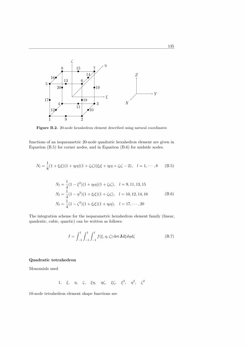
135
ξ
ζη
1 2
34
56
78
9
1011
12
1314
15
16
17 18
1920Y
Z
X
Figure B.2. 20-node hexahedron element described using natural coordinates
functions of an isoparametric 20-node quadratic hexahedron element are given inEquation (B.5) for corner nodes, and in Equation (B.6) for midside nodes.
Nl = 18(1 + ξlξ)(1 + ηlη)(1 + ζlζ)(ξlξ + ηlη + ζlζ − 2), l = 1, · · · , 8 (B.5)
Nl = 14(1− ξ2)(1 + ηlη)(1 + ζlζ), l = 9, 11, 13, 15
Nl = 14(1− η2)(1 + ξlξ)(1 + ζlζ), l = 10, 12, 14, 16
Nl = 14(1− ζ2)(1 + ξlξ)(1 + ηlη), l = 17, · · · , 20
(B.6)
The integration scheme for the isoparametric hexahedron element family (linear,quadratic, cubic, quartic) can be written as follows:
I =∫ 1
−1
∫ 1
−1
∫ 1
−1f(ξ, η, ζ) det Jdξdηdζ (B.7)
Quadratic tetrahedron
Monomials used
1, ξ, η, ζ, ξη, ηζ, ξζ, ξ2, η2, ζ2
10-node tetrahedron element shape functions are
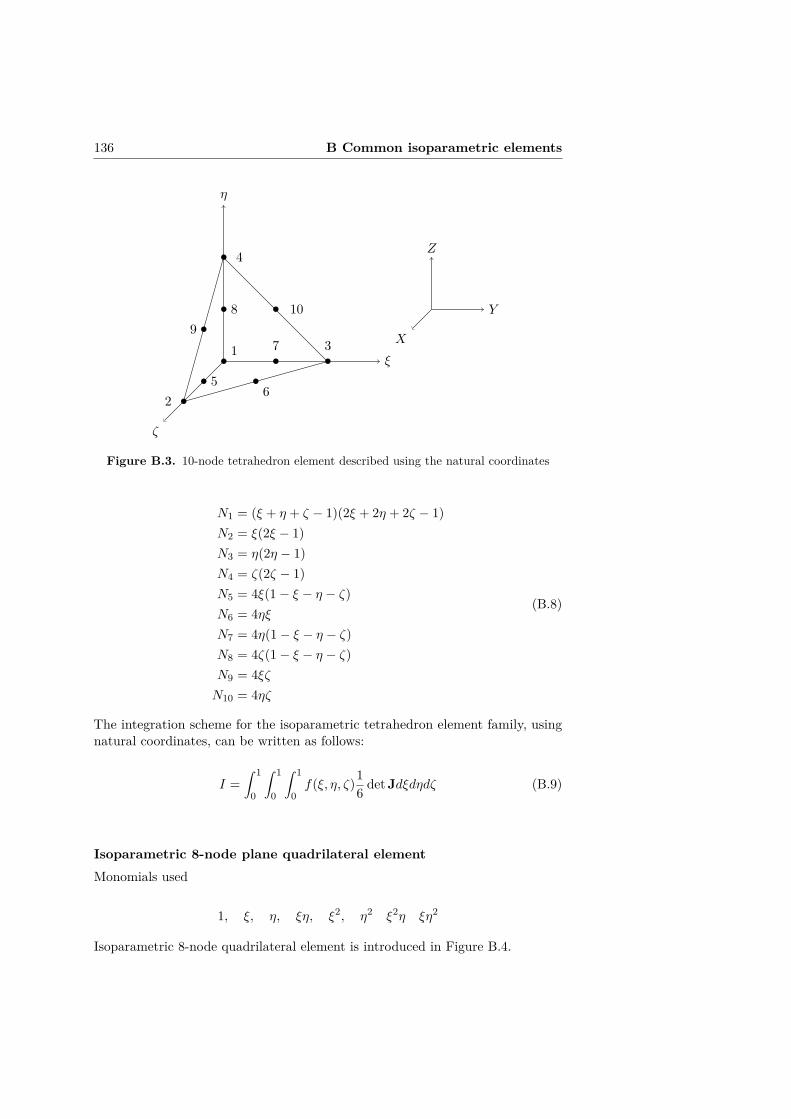
136 B Common isoparametric elements
ξ
η
ζ
1
2
3
4
56
7
89
10 Y
Z
X
Figure B.3. 10-node tetrahedron element described using the natural coordinates
N1 = (ξ + η + ζ − 1)(2ξ + 2η + 2ζ − 1)N2 = ξ(2ξ − 1)N3 = η(2η − 1)N4 = ζ(2ζ − 1)N5 = 4ξ(1− ξ − η − ζ)N6 = 4ηξN7 = 4η(1− ξ − η − ζ)N8 = 4ζ(1− ξ − η − ζ)N9 = 4ξζN10 = 4ηζ
(B.8)
The integration scheme for the isoparametric tetrahedron element family, usingnatural coordinates, can be written as follows:
I =∫ 1
0
∫ 1
0
∫ 1
0f(ξ, η, ζ)1
6 det Jdξdηdζ (B.9)
Isoparametric 8-node plane quadrilateral elementMonomials used
1, ξ, η, ξη, ξ2, η2 ξ2η ξη2
Isoparametric 8-node quadrilateral element is introduced in Figure B.4.
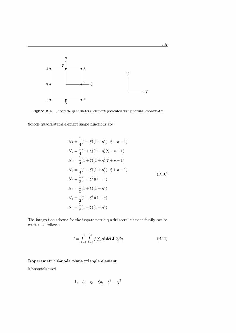
137
ξ
η
1 2
34
5
6
7
8
X
Y
Figure B.4. Quadratic quadrilateral element presented using natural coordinates
8-node quadrilateral element shape functions are
N1 = 14(1− ξ)(1− η)(−ξ − η − 1)
N2 = 14(1 + ξ)(1− η)(ξ − η − 1)
N3 = 14(1 + ξ)(1 + η)(ξ + η − 1)
N4 = 14(1− ξ)(1 + η)(−ξ + η − 1)
N5 = 12(1− ξ2)(1− η)
N6 = 12(1 + ξ)(1− η2)
N7 = 12(1− ξ2)(1 + η)
N8 = 12(1− ξ)(1− η2)
(B.10)
The integration scheme for the isoparametric quadrilateral element family can bewritten as follows:
I =∫ 1
−1
∫ 1
−1f(ξ, η) det Jdξdη (B.11)
Isoparametric 6-node plane triangle element
Monomials used
1, ξ, η, ξη, ξ2, η2
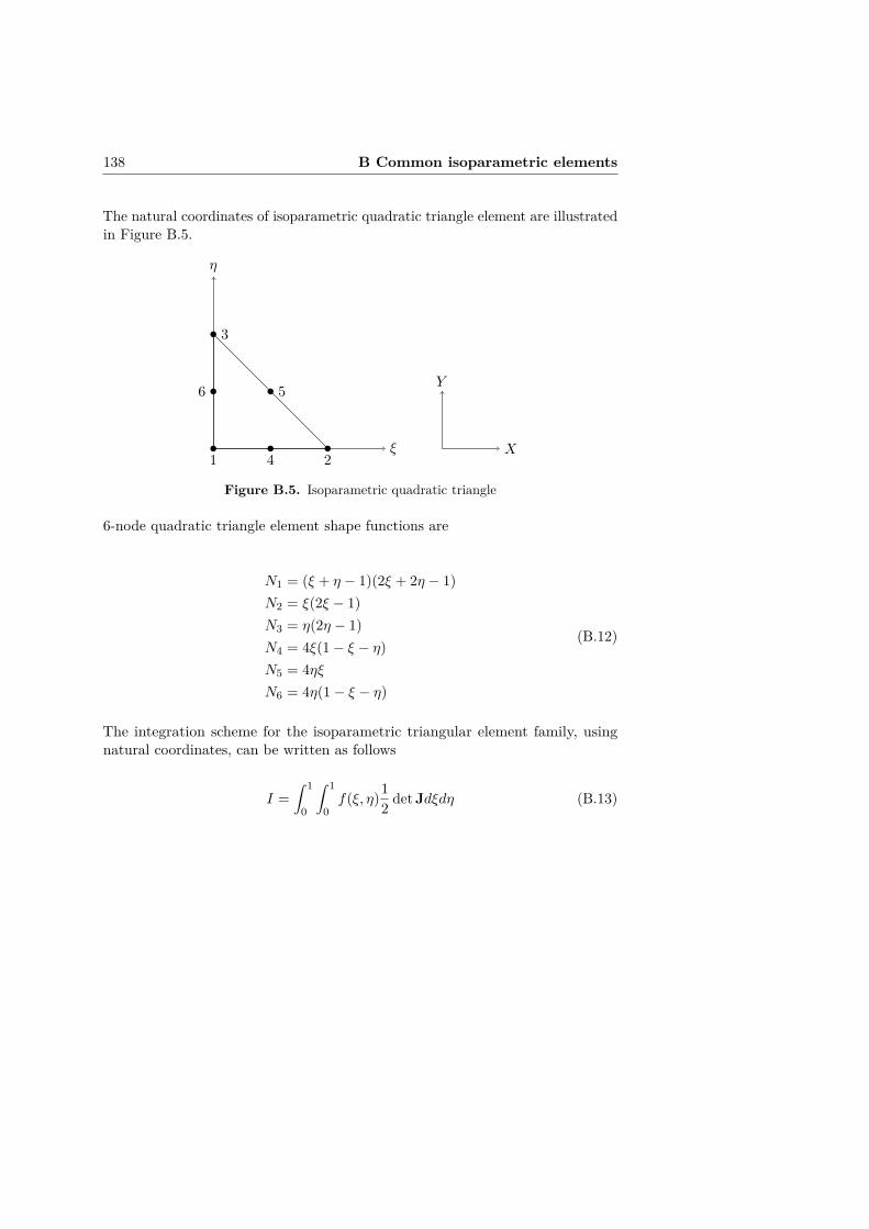
138 B Common isoparametric elements
The natural coordinates of isoparametric quadratic triangle element are illustratedin Figure B.5.
ξ
η
1 2
3
4
56
X
Y
Figure B.5. Isoparametric quadratic triangle
6-node quadratic triangle element shape functions are
N1 = (ξ + η − 1)(2ξ + 2η − 1)N2 = ξ(2ξ − 1)N3 = η(2η − 1)N4 = 4ξ(1− ξ − η)N5 = 4ηξN6 = 4η(1− ξ − η)
(B.12)
The integration scheme for the isoparametric triangular element family, usingnatural coordinates, can be written as follows
I =∫ 1
0
∫ 1
0f(ξ, η)1
2 det Jdξdη (B.13)
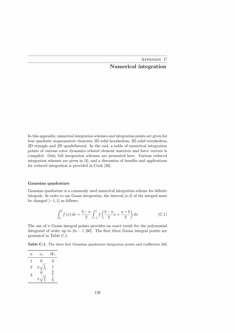
Appendix CNumerical integration
In this appendix, numerical integration schemes and integration points are given forfour quadratic isoparametric elements; 3D solid hexahedron, 3D solid tetrahedron,2D triangle and 2D quadrilateral. In the end, a table of numerical integrationpoints of various rotor dynamics related element matrices and force vectors iscompiled. Only full integration schemes are presented here. Various reducedintegration schemes are given in [4], and a discussion of benefits and applicationsfor reduced integration is provided in Cook [20].
Gaussian quadrature
Gaussian quadrature is a commonly used numerical integration scheme for definiteintegrals. In order to use Gauss integration, the interval [a, b] of the integral mustbe changed [−1, 1] as follows:
∫ b
af (x) dx = b− a
2
∫ 1
−1f
(b− a
2 x+ a+ b
2
)dx (C.1)
The use of n Gauss integral points provides an exact result for the polynomialintegrand of order up to 2n − 1 [60]. The first three Gauss integral points arepresented in Table C.1.
Table C.1. The three first Gaussian quadrature integration points and coefficients [60]
n xi Wi
1 0 22 ±
√13 1
3 0 89
±√
35
59
139

140 C Numerical integration
When applying Gaussian quadrature to isoparametric finite element expression,the integration interval is [−1, 1] by default, and when a sufficient number ofGauss points are used, Equation (C.1) can be written as follows:
∫ 1
−1f (x) dx =
n∑i=1
Wif (xi) (C.2)
where n is the number of used Gauss integration points, and Wi and xi are theweight coefficient and the value of the ith Gauss integration point.
Hexahedron elements
Hexahedron elements can be numerically integrated using the Gaussian quadraturerule, as follows:
I =n∑k=1
m∑j=1
l∑i=1
WkWjWif (ξi, ηj , ζk) (C.3)
Other integration rules also exist such as the 14-point rule introduced in [4].
Tetrahedron elements
For 10-node quadratic tetrahedron elements, the 4-point tetrahedron integrationrule can be written as follows:
I =4∑i=1
Wif (ξi, ηi, ζi) (C.4)
The 4-point tetrahedron integration rule coefficients are presented in Table C.2.Other tetrahedron rules exists depending on the number of element nodes.According to [4], the quadrature rule is possible for use for triangle and tetrahedronelements when using a special integration point distribution.
Table C.2. Isoparametric tetrahedron element 4-point integration points andcoefficients [4]
i ξi ηi ζi Wi
1 0.138196601125010 0.138196601125010 0.138196601125010 0.252 0.585410196624968 0.138196601125010 0.138196601125010 0.253 0.138196601125010 0.585410196624968 0.138196601125010 0.254 0.138196601125010 0.138196601125010 0.585410196624968 0.25

141
Quadrilateral elements
Quadrilateral elements can be numerically integrated using the Gaussian quadraturerule, as follows:
I =m∑j=1
l∑i=1
WjWif (ξi, ηj) (C.5)
For visualization, the 3×3 two-dimensional Gaussian quadrature integration pointlocations are presented in Figure C.1.
ξ
η
1 2
34
5
6
7
8
1 5 2
8 9 64 7 3 Node point
Integration point
Figure C.1. The 3× 3 Gaussian quadrature point locations
Triangle elements
For the 6-node triangle element, the 3-point triangle integration rule can bewritten as follows:
∫ 1
0
∫ 1
0f (ξ, η) =
3∑i=1
Wif (ξi, ηi) (C.6)
The 3 point triangle integration rule coefficients are given in Table C.3, and thepoints are visualized in Figure C.2.
Table C.3. Isoparametric triangle element 3-point integration points andcoefficients [2, 4]
i 1 2 3ξi 1/6 2/3 1/6ηi 1/6 1/6 2/3wi 1/3 1/3 1/3
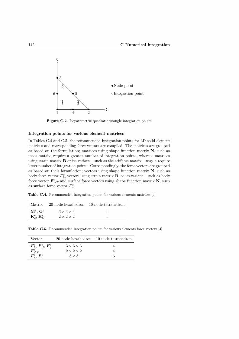
142 C Numerical integration
ξ
η
1 2
3
4
56
1 2
3 Node point
Integration point
Figure C.2. Isoparametric quadratic triangle integration points
Integration points for various element matrices
In Tables C.4 and C.5, the recommended integration points for 3D solid elementmatrices and corresponding force vectors are compiled. The matrices are groupedas based on the formulation; matrices using shape function matrix N, such asmass matrix, require a greater number of integration points, whereas matricesusing strain matrix B or its variant – such as the stiffness matrix – may a requirelower number of integration points. Correspondingly, the force vectors are groupedas based on their formulation; vectors using shape function matrix N, such asbody force vector F e
b, vectors using strain matrix B, or its variant – such as bodyforce vector F e
∆T and surface force vectors using shape function matrix N, suchas surface force vector F e
s.
Table C.4. Recommended integration points for various elements matrices [4]
Matrix 20-node hexahedron 10-node tetrahedronMe, Ge 3× 3× 3 4Kee, Ke
G 2× 2× 2 4
Table C.5. Recommended integration points for various elements force vectors [4]
Vector 20-node hexahedron 10-node tetrahedronF eb, F e
Ω, F eg 3× 3× 3 4
F e∆T 2× 2× 2 4
F es, F e
p 3× 3 6

ACTA UNIVERSITATIS LAPPEENRANTAENSIS
782. SIPILÄ, JENNI. The many faces of ambivalence in the decision-making process. 2017.Diss.
783. HAN, MEI. Hydrodynamics and mass transfer in airlift bioreactors; experimental andnumerical simulation analysis. 2017. Diss.
784. ESCALANTE, JOHN BRUZZO. Dynamic simulation of cross-country skiing. 2017. Diss.
785. NOKKA, JARKKO. Energy efficiency analyses of hybrid non-road mobile machinery byreal-time virtual prototyping. 2018. Diss.
786. VUORIO, ANNA. Opportunity-specific entrepreneurial intentions in sustainableentrepreneurship. 2018. Diss.
787. PULKKINEN, AKI. Towards a better understanding of activity and selectivity trendsinvolving K and O adsorption on selected metal surfaces. 2017. Diss.
788. ZHAO, WENLONG. Reliability based research on design, analysis and control of theremote handling maintenance system for fusion reactor. 2018. Diss.
789. IAKOVLEVA, EVGENIA. Novel sorbents from low-cost materials for water treatment.2018. Diss.
790. KEDZIORA, DAMIAN. Service offshoring industry: systems engineering approach to itstransitional challenges. 2018. Diss.
791. WU, JING. Soft computing methods for performance improvement of EAMA robot infusion reactor application. 2018. Diss.
792. VOSTATEK, PAVEL. Blood vessel segmentation in the analysis of retinal anddiaphragm images. 2018. Diss.
793. AJO, PETRI. Hydroxyl radical behavior in water treatment with gas-phase pulsedcorona discharge. 2018. Diss.
794. BANAEIANJAHROMI, NEGIN. On the role of enterprise architecture in enterpriseintegration. 2018. Diss.
795. HASHEELA-MUFETI, VICTORIA TULIVAYE. Empirical studies on the adoption andimplementation of ERP in SMEs in developing countries. 2018. Diss.
796. JANHUNEN, SARI. Determinants of the local acceptability of wind power in Finland.2018. Diss.
797. TEPLOV, ROMAN. A holistic approach to measuring open innovation: contribution totheory development. 2018. Diss.
798. ALBATS, EKATERINA. Facilitating university-industry collaboration with a multi-levelstakeholder perspective. 2018. Diss.
799. TURA, NINA. Value creation for sustainability-oriented innovations: challenges andsupporting methods. 2018. Diss.
800. TALIKKA, MARJA. Recognizing required changes to higher education engineeringprograms' information literacy education as a consequence of research problemsbecoming more complex. 2018. Diss.

801. MATTSSON, ALEKSI. Design of customer-end converter systems for low voltage DCdistribution from a life cycle cost perspective. 2018. Diss.
802. JÄRVI, HENNA. Customer engagement, a friend or a foe? Investigating the relationshipbetween customer engagement and value co-destruction. 2018. Diss.
803. DABROWSKA, JUSTYNA. Organizing for open innovation: adding the human element.2018. Diss.
804. TIAINEN, JONNA. Losses in low-Reynolds-number centrifugal compressors. 2018.Diss.
805. GYASI, EMMANUEL AFRANE. On adaptive intelligent welding: Technique feasibility inweld quality assurance for advanced steels. 2018. Diss.
806. PROSKURINA, SVETLANA. International trade in biomass for energy production: Thelocal and global context. 2018. Diss.
807. DABIRI, MOHAMMAD. The low-cycle fatigue of S960 MC direct-quenched high-strength steel. 2018. Diss.
808. KOSKELA, VIRPI. Tapping experiences of presence to connect people andorganizational creativity. 2018. Diss.
809. HERALA, ANTTI. Benefits from Open Data: barriers to supply and demand of OpenData in private organizations. 2018. Diss.
810. KÄYHKÖ, JORMA. Erityisen tuen toimintaprosessien nykytila ja kehittäminensuomalaisessa oppisopimuskoulutuksessa. 2018. Diss.
811. HAJIKHANI, ARASH. Understanding and leveraging the social network services ininnovation ecosystems. 2018. Diss.
812. SKRIKO, TUOMAS. Dependence of manufacturing parameters on the performancequality of welded joints made of direct quenched ultra-high-strength steel. 2018. Diss.
813. KARTTUNEN, ELINA. Management of technological resource dependencies ininterorganizational networks. 2018. Diss.
814. CHILD, MICHAEL. Transition towards long-term sustainability of the Finnish energysystem. 2018. Diss.
815. NUTAKOR, CHARLES. An experimental and theoretical investigation of power losses inplanetary gearboxes. 2018. Diss.
816. KONSTI-LAAKSO, SUVI. Co-creation, brokering and innovation networks: A model forinnovating with users. 2018. Diss.
817. HURSKAINEN, VESA-VILLE. Dynamic analysis of flexible multibody systems usingfinite elements based on the absolute nodal coordinate formulation. 2018. Diss.
818. VASILYEV, FEDOR. Model-based design and optimisation of hydrometallurgical liquid-liquid extraction processes. 2018. Diss.
819. DEMESA, ABAYNEH. Towards sustainable production of value-added chemicals andmaterials from lignocellulosic biomass: carboxylic acids and cellulose nanocrystals.2018. Diss.


Eerik Sikanen
DYNAMIC ANALYSIS OF ROTATING SYSTEMSINCLUDING CONTACT AND THERMAL-INDUCEDEFFECTS
Acta Universitatis Lappeenrantaensis
820
Acta Universitatis Lappeenrantaensis
820
ISBN 978-952-335-284-1 ISBN 978-952-335-285-8 (PDF)ISSN-L 1456-4491ISSN 1456-4491Lappeenranta 2018