Numerical studies in rotating and stratified turbulence

Numerical studies in rotating and stratifiedturbulence

by

Enrico Deusebio

December 2013Technical Report

Royal Institute of TechnologyDepartment of Mechanics

SE-100 44 Stockholm, Sweden

Akademisk avhandling som med tillstand av Kungliga Tekniska Hogskolan iStockholm framlagges till o!entlig granskning for avlaggande av teknologiedoktorsexamen fredagen den 17 januari 2014 kl 10.00 i Kollegiesalen, Kung-liga Tekniska Hogskolan, Brinellvagen 8, Stockholm.

c!Enrico Deusebio 2013

Tryckt av Eprint AB 2013

Numeriska simuleringar av roterande och stratifierad tur-bulens

Enrico DeusebioLinne Flow Centre, KTH Mechanics, Royal Institute of TechnologySE-100 44 Stockholm, Sweden

SammanfattningEn grundlig vetenskaplig forstaelse av turbulens saknas fortfarande, fastanfenomenet har studerats i fem hundra ar. Vid sidan av observationer och ex-periment kan berakningar med hjalp av kraftfulla datorer idag ge oss en delinsikter i turbulensens dynamik. I denna avhandling presenteras simuleringarav saval homogen turbulens som turbulens i stromningar i narvaro av en vagg.I bada fallen studeras en roterande och stratifierad fluid, sa som ar fallet igeofysikaliska stromningar dar jordrotationen och den vertikala densitetsvaria-tionen har stort inflytande.

For homogen turbulens undersoker vi hur energiutbytet mellan olika turbulentaskalor paverkas av stark men andlig rotation och stratifiering. Till skillnad frankvasigeostrofisk turbulens, visar vi att det existerar en energikaskad mot min-dre skalor som initieras vid den skala vid vilken turbulensen exciteras. Vidstora skalor ar denna process av underordnad betydelse, men vid mindre skalorkommer den att dominera. Vid dessa skalor ser man darfor att vagtalsspek-trum av den turbulenta energin genomgar en overgang fran k!3 till k!5/3.Tvapunktsstatistik visar en god overenstammelse med matningar fran atmos-faren, vilket talar for att energikaskaden mot mindre skalor ar en betydelsefullprocess i atmosfaren.

Ett gransskikt i ett roterande system i vilket rotationsaxeln ar normal motvaggen brukar kallas ett Ekmanskikt, vilket kan ses som en modell for degransskikt som utvecklar sig i atmosfaren och oceanerna. Vi studerar denturbulenta dynamiken i Ekmanskiktet med hjalp av numeriska simuleringar,med speciellt fokus pa de strukturer som utvecklas vid mattliga Reynoldstal.For neutralt skiktade fluider visar vi att det finns en turbulent kaskad av he-licitet i det logaritmiska skiktet. Vi fokuserar ocksa pa e!ekten av en stabilskiktning som uppstar pa grund av en vertikal temperaturgradient. Om skikt-ningen inte ar alltfor stark, observerar vi en turbulent dynamik som i stort settoverenstammer med existerande teorier och modeller som anvands for atmos-fariska gransskikt. For starkare skiktning visar vi att det finns samexisterandeturbulenta och laminara omraden som visar sig i snett lopande band i forhal-lande till medelhastigheten, i stor likhet med vad som nyligen observerats iandra stromningar som genomgar transition mellan ett laminart och turbulenttillstand.

iii

Numerical studies in rotating and stratified turbulence

Enrico DeusebioLinne Flow Centre, KTH Mechanics, Royal Institute of TechnologySE-100 44 Stockholm, Sweden

AbstractAlthough turbulence has been studied for more than five hundred years, a thor-ough understanding of turbulent flows is still missing. Nowadays computingpower can o!er an alternative tool, besides measurements and experiments,to give some insights into turbulent dynamics. In this thesis, numerical sim-ulations are employed to study homogeneous and wall-bounded turbulence inrotating and stably stratified conditions, as encountered in geophysical flowswhere the rotation of the Earth as well as the vertical density variation influencethe dynamics.

In the context of homogeneous turbulence, we investigate how the transfer ofenergy among scales is a!ected by the presence of strong but finite rotation andstratification. Unlike geostrophic turbulence, we show that there is a forwardenergy cascade towards small scales which is initiated at the forcing scales.The contribution of this process to the general dynamic is secondary at largescales but becomes dominant at smaller scales where it leads to a shallowingof the energy spectrum, from k!3 to k!5/3. Two-point statistics show a goodagreement with measurements in the atmosphere, suggesting that this processis an important mechanism for energy transfer in the atmosphere.

Boundary layers subjected to system rotation around the wall-normal axis areusually referred to as Ekman layers and they can be seen as a model of theatmospheric and oceanic boundary layers developing at mid and high latitudes.We study the turbulent dynamics in Ekman layers by means of numerical sim-ulations, focusing on the turbulent structures developing at moderately highReynolds numbers. For neutrally stratified conditions, we show that there ex-ists a turbulent helicity cascade in the logarithmic region. We focus on the e!ectof a stable stratification produced by a vertical positive temperature gradient.For moderate stratification, continuously turbulent regimes are produced whichare in fair agreement with existing theories and models used in the context ofatmospheric boundary layer dynamics. For larger degree of stratification, weshow that laminar and turbulent motions coexist and displace along inclinedpatterns similar to what has been recently observed in other transitional flows.

Descriptors: Geostrophic turbulence, stable stratification, rotation, wall-bounded turbulence, gravity waves, atmospheric dynamics, direct numericalsimulations

iv

Preface

This thesis contains numerical investigations of stratified and rotating turbu-lence, both with and without the presence of walls. A brief introduction onthe basic concepts and methods is presented in the first part. The second partcontains six articles and one internal report. The papers are adjusted to com-ply with the present thesis format for consistency, but their contents have notbeen altered as compared with their original counterparts.

Paper I. A. Vallgren, E. Deusebio & E. Lindborg, 2011Possible explanation of the atmospheric kinetic and potential energy spectra.Phys. Rev. Lett., 107:26, 268501.

Paper II. E. Deusebio, A. Vallgren & E. Lindborg, 2013The route to dissipation in strongly stratified and rotating flows. J. FluidMech., 720, 66-103, 2013

Paper III. E. Deusebio, A. Augier & E. Lindborg, 2013Third order structure functions in rotating and stratified turbulence: analyticaland numerical results compared with data from the stratosphere. Submitted toJ. Fluid Mech.

Paper IV. E. Deusebio, G. Boffetta, S. Musacchio & E. Lindborg,2013Dimensional transition in rotating turbulence Submitted to Phys. Rev. E

Paper V. E. Deusebio, G. Brethouwer, P. Schlatter & E. Lindborg,2013A numerical study of the unstratified and stratified Ekman layer. Under revi-sion for publication in J. Fluid Mech.

Paper VI. E. Deusebio & E. Lindborg, 2013Helicity in the Ekman boundary layer. Submitted to J. Fluid Mech. Rapids

Paper VII. E. Deusebio, 2012The open-channel version of SIMSON Internal Report

v

Division of work among authorsThe main advisor for the project is Dr. Erik Lindborg (EL). Dr. PhilippSchlatter (PS) and Dr. Geert Brethouwer (GB) have acted as co-advisors.

Paper IThe code was developed and implemented by Andreas Vallgren (AV) and EnricoDeusebio (ED). The numerical simulations were performed by AV. The paperwas written by EL, with the help of AV and ED. ED was particularly activeduring the review process.

Paper IIThe solver code was developed and implemented by ED in collaboration withAV. The numerical simulations were performed by ED. The post-processingcode for studying the triad interactions was developed by ED. The paper waswritten by ED, with the help of EL. AV provided comments on the article.

Paper IIIThe simulations and the post-processing were carried out by ED with inputfrom EL and Pierre Augier (PA). The paper was written by ED, EL and PA.

Paper IVThe code which has been used in the study was provided by Guido Bo!etta(GB) and Stefano Musacchio (SM). ED implemented an implicit scheme foradding the contribution of rotation and for I/O operations. ED carried out thesimulations with input from GB and SM. The paper was written by GB, SMand ED with feedback from EL.

Paper VThe modification of the existing code SIMSON was performed by ED, with thehelp of PS and GB. The simulations and the analysis of the results were doneby ED, with the input of PS, GB and EL. The paper was written by ED, withfeedback by EL, GB and PS.

Paper VIThe post-processing of the data was done by ED with input from EL. Thepaper was written by ED, with feedback by EL.

Paper VIIThe idea underlying the new discretisation was suggested by EL. The implemen-tation, code-optimisation and validation were done by ED, under supervisionof PS, GB and EL. The report was written by ED.

vi

Part of the work has also been presented at the following international confer-ences:

E. Deusebio, A. Vallgren & E. LindborgQuasi-geostrophic turbulence at finite Rossby number. 7th International Sym-posium of Stratified Flows - Rome 2011.

E. Deusebio, P. Schlatter, G. Brethouwer & E. LindborgDirect numerical simulations of stratified open-channel flows. 13th EuropeanTurbulence Conference - Warsaw 2011.

A. Vallgren, E. Deusebio & E. LindborgQuasi-geostrophic turbulence at finite Rossby number. 13th European Turbu-lence Conference - Warsaw 2011.

E. Deusebio & E. LindborgThe role of geostrophy and ageostrophy in rotating and stratified systems. 9th

European Fluid Mechanics Conference - Rome 2012.

E. Deusebio & E. LindborgPathways to dissipation in strongly rotating and stratified turbulent systems.65th Annual Meeting of the APS Division of Fluid Dynamics - San Diego, 2012.

E. Deusebio, P. Schlatter, G. Brethouwer & E. LindborgDirect numerical investigation of the stably-stratified Ekman layer. 14th Euro-pean Turbulence Conference - Lyon, 2013.

vii

Perche tu non perda mai la direzione, e perche, se mai la perdessi,questo ti guidi verso le persone che ti vogliono bene (N. Mok-bel)

ix

Sammanfattning iii

Abstract iv

Preface v

Part I - Introduction 1

Chapter 1. Turbulence and numerical simulations 3

Chapter 2. Rotating and stratified turbulence: a geophysicalperspective 8

2.1. Geostrophic turbulence 9

2.2. Stratified turbulence 12

2.3. Three-dimensional turbulence 13

2.4. Rotating turbulence 14

2.5. Towards the atmosphere... 17

Chapter 3. Stratified and rotating turbulence in the presence ofwalls 22

3.1. The scales of motions in wall-bounded turbulence 22

3.2. Numerical grids in wall-bounded flows 26

3.3. Rotating wall-bounded flows 27

3.4. Stratified wall-bounded flows 31

Chapter 4. Summary of the papers 37

4.1. Homogeneous turbulence close to geostrophic conditions 37

4.2. Wall bounded stratified turbulence 38

Chapter 5. Conclusions and outlook 41

5.1. Turbulence close to geostrophy: A key for improving weatherforecast... 41

5.2. Wall-bounded turbulence and atmospheric boundary layers 43

Acknowledgments 45

Bibliography 47

Part II - Papers 57

Possible explanation of the atmospheric kinetic and potentialenergy spectra 61

The route to dissipation in strongly stratified and rotating flows 73

xi

Third order structure function in rotating and stratified turbulence:analytical and numerical results compared with datafrom the stratosphere 119

Dimensional transition in rotating turbulence 141

A numerical study of the unstratified and stratified Ekman layer 157

Helicity in the Ekman boundary layer 199

The open-channel version of SIMSON 213

Part I

Introduction

CHAPTER 1

Turbulence and numerical simulations

“Observe the motion of the surface of the water which resembles that of hair,and has two motions, of which one goes on with the flow of the surface, theother forms the lines of the eddies; thus the water forms eddying whirlpoolsone part of which are due to the impetus of the principal current and the otherto the incidental motion and return flow1.” It was between the XV and theXVI century that the first attempt of a scientific study of turbulent motions wasdone by the Italian Leonardo da Vinci. More than five hundred years later, tur-bulence is still not fully understood and many of its aspects remain mysterious.Richard Feynman describes turbulence as one of the most important unsolvedproblem of classical physics (Feynman 1964). The note left by Leonardo daVinci already contains a description of some important characteristic featuresof turbulence: the presence of eddies and swirling motions which, in a ratherchaotic manner, superimpose on the main motion of the fluid. It was the sameobservation which led Reynolds (1895), almost four hundred years later, to de-scribe turbulent motions statistically by decomposing the velocity field into amean and a fluctuating part. Indeed, the perhaps most important insight intothe essentials of turbulence goes back to less than a hundred years ago, withthe observations of Richardson (1922)

Big whirls have little whirlsthat feed on their velocity,and little whirls have lesser whirlsand so on to viscosity

Far from being trivial, Richardson’s observation constitutes the ground onwhich all the following theories were based (e.g. Kolmogorov 1941a). Largeeddies break down into smaller eddies in an inviscid process which continuesuntil kinetic energy is converted into heat at the very smallest scales of motionswhere viscosity dominates. Thus, turbulent flows possess many scales, both inspace and in time, and they own their intrinsic complexity to the interplayamong these scales.

From a historical perspective, most of the advances in the understandingof turbulent processes were made in the past hundred years, since the pioneerwork of Reynolds (1886). Besides the experimental investigations, a substantial

1see Richter, J. P. 1970. Plate 20 and Note 389. In The Notebooks of Leonardo Da Vinci.New York: Dover Publications.

3

4 1. TURBULENCE AND NUMERICAL SIMULATIONS

Figure 1.1. da Vinci sketch of a turbulent flow

amount of work has also been dedicated to theoretical investigations of turbu-lence. Several approaches were proposed and undertaken. Strongly influencedby the view of turbulent motions as chaotic and unpredictable, the early studiesmainly aimed at a statistical characterization of the dynamics.

Perhaps the most important contribution to a quantitative statistical de-scription of turbulent flows is the theory proposed by Kolmogorov (1941a). Aseddies break down into smaller eddies, they lose any preferable orientation andthe anisotropy of the large scales of the flow is progressively lost. Kolmogorov(1941a) suggested that statistical quantities in the cascade neither depend onthe direction nor on the spatial coordinates, but they attain an universal formwhich depends only on the energy flux through the cascade, !, and, at smallscales, on the viscosity ". Despite its simplicity, Kolmogorov (1941a) theoryhas been able to make quantitatively accurate predictions.

The apparent chaotic and unpredictable nature of turbulent flows seemsto be in contrast with the deterministic nature of the Navier-Stokes equationswhich govern the fluid motions. Besides the statistical approach, other ap-proaches have also been proposed, postulating the presence of more organizedpatterns. The structural approach aims at identifying coherent structures whichcyclically appears in the flow and sustain the turbulent motions. The deter-ministic approach, on the other hand, views a turbulent process as a nonlineardynamical system which exhibits a high dependence on initial conditions andapparently chaotic solutions which, however, project onto particular objects inphase-space, called “strange attractors”.

In the last fifty years turbulence research has benefited from the powerfultool of digital computers, which complementary to experiments, can be used

1. TURBULENCE AND NUMERICAL SIMULATIONS 5

to study turbulence in detail. This thesis shows how such an approach canbe e!ectively employed in order to shed light on turbulent dynamics. As op-posed to experiments, numerical simulations give full information of flow fieldsand also allow a perfect control of external conditions (e.g. boundary con-ditions). Moreover, they also allow us to study idealized and “non-physical“setups where di!erent factors/phenomena influencing the turbulent dynamicscan be separated.

The first attempt to carry out a direct flow computation was made in thebeginning of the XX century by Richardson (1922), who undertook the firsthistorical weather forecast ever done. The measured atmospheric data wereadvanced in time by using a rather simple mathematical model able to capturethe main features of the atmosphere, predicting the flow evolution in the nextsix hours. All the computations were done by hand. Unfortunately, becausesome smoothing techniques were not applied on the original data, Richardson’sforecast failed dramatically. Nevertheless, it represents a mile-stone in thesoon-to-appear era of numerical simulations.

It was only in the beginning of the 1960 that the technology of the digitalcomputers were su"ciently developed to allow for the first numerical compu-tations. Lorenz (1963) studied a simple version of the Navier-Stokes equationsin his pioneer work based on machine computations. The system studied byLorenz (1963) was nonlinear and deterministic, as the Navier-Stokes equations.Moreover, it shared some common features with turbulent motions, such as highsensitivity to initial conditions and chaotic solutions. The work of Lorenz re-solved the apparent paradox that deterministic systems can behave chaotically,delineating the beginning of the modern view of turbulence as “deterministicchaos”.

From a numerical perspective, the most challenging aspect of turbulenceis its intrinsic feature of containing a large range of scales that interact witheach other. If one aims at correctly simulating turbulent flows, all the scales,from the large energy-containing scales to the very smallest scales, must berepresented, posing severe computational requirements. In the atmosphere, forinstance, the largest scales are of the order of thousand kilometres. On theother hand, viscosity acts at millimetre scales. To represent such a vast span ofscales in a simulation is, of course, impossible. Also numerical computations ofturbulent flows in typical engineering applications, such as flows around aircraftor cars, are still out of reach. The largest scale of turbulence is often referredto as the integral length scale L, whereas the smallest scale is the Kolmogorovscale, defined as # = "3/4/!1/4. The Kolmogorov scale is usually interpretedas the scale at which viscosity acts and dissipates the downscale-cascadingenergy. A fundamental parameter in fluid dynamic applications is the Reynoldsnumber, Re = UL/", which quantifies the relative importance between inertialand viscous forces. Here, U is a characteristic large scale velocity. The ratiobetween the largest scale, L, and the smallest viscosity a!ected scale, #, can berelated to the Reynolds number as L/# " Re3/4. Values of Re are typically of

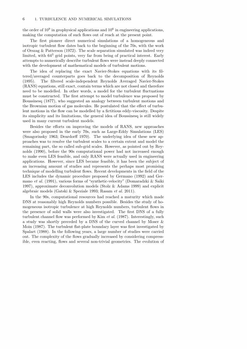
6 1. TURBULENCE AND NUMERICAL SIMULATIONS

the order of 109 in geophysical applications and 106 in engineering applications,making the computation of such flows out of reach at the present point.

The first pioneer direct numerical simulations of a homogeneous andisotropic turbulent flow dates back to the beginning of the 70s, with the workof Orszag & Patterson (1972). The scale separation simulated was indeed verylimited, with 643 grid points, very far from being of practical interest. Earlyattempts to numerically describe turbulent flows were instead deeply connectedwith the development of mathematical models of turbulent motions.

The idea of replacing the exact Navier-Stokes equations with its fil-tered/averaged counterparts goes back to the decomposition of Reynolds(1895). The filtered scale-independent Reynolds Averaged Navier-Stokes(RANS) equations, still exact, contain terms which are not closed and thereforeneed to be modelled. In other words, a model for the turbulent fluctuationsmust be constructed. The first attempt to model turbulence was proposed byBoussinesq (1877), who suggested an analogy between turbulent motions andthe Brownian motion of gas molecules. He postulated that the e!ect of turbu-lent motions in the flow can be modelled by a fictitious eddy-viscosity. Despiteits simplicity and its limitations, the general idea of Boussinesq is still widelyused in many current turbulent models.

Besides the e!orts on improving the models of RANS, new approacheswere also proposed in the early 70s, such as Large-Eddy Simulations (LES)(Smagorinsky 1963; Deardor! 1970). The underlying idea of these new ap-proaches was to resolve the turbulent scales to a certain extent and model theremaining part, the so called sub-grid scales. However, as pointed out by Rey-nolds (1990), before the 90s computational power had not increased enoughto make even LES feasible, and only RANS were actually used in engineeringapplications. However, since LES became feasible, it has been the subject ofan increasing amount of studies and represents the perhaps most promisingtechnique of modelling turbulent flows. Recent developments in the field of theLES includes the dynamic procedure proposed by Germano (1992) and Ger-mano et al. (1991), various forms of “synthetic-velocity” (Domaradzki & Saiki1997), approximate deconvolution models (Stolz & Adams 1999) and explicitalgebraic models (Gatski & Speziale 1993; Rasam et al. 2011).

In the 90s, computational resources had reached a maturity which madeDNS at reasonably high Reynolds numbers possible. Besides the study of ho-mogeneous isotropic turbulence at high Reynolds numbers, turbulent flows inthe presence of solid walls were also investigated. The first DNS of a fullyturbulent channel flow was performed by Kim et al. (1987). Interestingly, sucha study was shortly preceded by a DNS of the curved channel by Moser &Moin (1987). The turbulent flat-plate boundary layer was first investigated bySpalart (1988). In the following years, a large number of studies were carriedout. The complexity of the flows gradually increased by considering compress-ible, even reacting, flows and several non-trivial geometries. The evolution of

1. TURBULENCE AND NUMERICAL SIMULATIONS 7

the geometries also led to the development of new numerical methods able todeal with curved and irregular walls.

Nevertheless, as noted by Moin & Mahesh (1998), it was still impossibleto simulate flows with Reynolds numbers comparable to experiments. Thedevelopment of massively parallel machines over the last decade has made itfeasible to increase the Reynolds number by almost one order of magnitude. Inthe field of isotropic and homogeneous turbulence, a DNS at resolution 40963

was performed by Kaneda et al. (2003). In the field of wall-bounded flows, asimulation of a channel flow at a friction Reynolds number2 Re! = 2000 wasperformed by Hoyas & Jimenez (2006), whereas its turbulent boundary layercounterparts were studied by Schlatter et al. (2009) at a Re", defined with themomentum thickness3 $ in place of L, of Re" = 2500 and Sillero et al. (2013) atRe" = 6000. Nowadays, the Reynolds number that can be reached in numeri-cal simulations and in experiments are comparable, allowing for a comparisonand a complementary analysis (Schlatter & Orlu 2010; Segalini et al. 2011).More importantly, the increase of the Reynolds number allows us to gain im-portant insights in the turbulent dynamics, revealing important features, suchas intermittency (Benzi et al. 1993; Frisch 1996; Biferale & Toschi 2001), thepresence of coherent structures (Del Alamo et al. 2006) and interactions amongthe di!erent scales of the flow (Hoyas & Jimenez 2006; Mathis et al. 2011).

In the spirit of the discussion above, in this thesis we aim at studyingthe turbulent dynamics in the presence of rotation and stratification by meansof high-resolution numerical simulations. Such conditions are very important,especially in a geophysical perspective. A thorough understanding of turbu-lent processes should mainly focus on how energy is exchanged among di!er-ent scales. This is important both from a scientific and a practical point ofview. Critical evaluations as well as related improvements of large-scale atmo-spheric and oceanic models cannot be achieved unless the physics and the mainmechanisms underlying atmospheric and oceanic dynamics are understood. Inchapter 2, a short survey of the background on turbulence strongly a!ectedby rotation and stratification is given. Chapter 3 presents a short overviewon wall-bounded turbulence and on the e!ect of system rotation and stablestratification. In chapter 4, a summary of the main findings is o!ered. Finally,chapter 5 concludes with some general remarks and outlooks.

2defined as Re! = u!L/!. u! =!"w/# is the friction velocity with "w being the shear stress

at the wall.3defined as

"!0

#1! u

U!

$u

U!dy.

CHAPTER 2

Rotating and stratified turbulence: a geophysicalperspective

Atmospheric and oceanic flows are highly a!ected by both rotation and strat-ification. Rotation is exerted through Coriolis forces which mainly act in hori-zontal planes whereas stratification largely a!ects the motion along the verti-cal direction through the Archimede’s force. Depending on the mean densityprofile, stratification can either enhance or suppress vertical motions. Strati-fication in the atmosphere is usually stable above the boundary layer (Vallis2006; Gill 1982), i.e. a fluid particle which is displaced in the vertical direc-tion tends to return to its initial position. Whereas highly rotating flows tendto form structures which are elongated in the vertical direction (Taylor 1923),highly stratified flows favour thin structures elongated in the horizontal direc-tion. Such structures are usually referred to as pancake structures (Lindborg2006; Brethouwer et al. 2007). It is the interplay between these two regimesthat gives rise to the variety of dynamics seen in the atmosphere.

In the most general case, the governing equations for the flows in the atmo-sphere and in the oceans are the compressible Navier-Stokes equations. Fluiddensity may change from place to place, a!ected by other scalar quantitiessuch as pressure, temperature, humidity and salinity. Nevertheless, a good in-sight into the turbulent dynamics can be gained by reducing the complexity ofthe problem by making a few assumptions. Following the standard derivation,we restrict ourselves to the incompressible Navier-Stokes equations under theBoussinesq approximation on a f -plane. These can be written as

Du

Dt= #$p

%0# fez % u+ bez, (2.1a)

Db

Dt= #N2w, (2.1b)

$ · u = 0 , (2.1c)

where u is the velocity vector, f = 2# is the Coriolis parameter with # beingthe rotation rate in the f -plane, ez is the vertical unit vector, p is the pressure

and D/Dt represents the material derivative. N =!g%!1

0 d%/dz is the Brunt-

Vaisala frequency, with g being the gravity acceleration, %0 a reference densityand d%/dz the background density vertical gradient, and b = g%/%0 is thebuoyancy, where % is the fluctuating density. In general, b = b(T, S), where T

8

2.1. GEOSTROPHIC TURBULENCE 9

is the (potential) temperature and S the salinity. In the following, however, wewill assume for simplicity that only T a!ects b and therefore that b = gT/T0

(Vallis 2006). In (2.1) we have omitted di!usion terms which act only at verysmall scales. In the following sections, we simplify this system for the di!erentatmospheric and oceanic regimes, shortly reviewing the main theories and themain open questions concerning turbulence in geophysical flows.

2.1. Geostrophic turbulence

Atmospheric and oceanic dynamics are forced at very large scales. In the at-mosphere, available potential energy associated with the poleward temperaturegradient is converted to kinetic energy by baroclinic instability which developson scales of the order of thousand kilometres. The general circulation of theoceans is mainly driven by surface fluxes of momentum at similar spatial scales.At such large scales, Earth rotation strongly a!ects the flow. Moreover, thestratification is generally quite strong, both in the atmosphere and in the oceans(Pedlosky 1987; Vallis 2006).

The relative importance of Coriolis forces and buoyancy forces comparedto inertial forces are often quantified by the Rossby and the Froude numbers,defined as

Ro =U

fLand Fr =

U

NL. (2.2)

Here, L is a characteristic horizontal scale and U a characteristic velocity.Note that the use of a horizontal length scale rather than a vertical lengthscale in the definition of Fr is not standard in geophysical sciences (see e.g.Gill 1982). However, as will be discussed in the following, recent advancementsin the understanding of stratified turbulence suggest that the Froude numberdefined with a vertical length scale always remains of the order of unity, even instrongly stratified regimes (Billant & Chomaz 2001). On the other hand, Fr,defined as in (2.2), is in most geophysical applications a small parameter. In theatmosphere, typical values of Fr are of the order of 10!3 and typical values ofRo are of the order of 10!1 (Deusebio et al. 2013b). Thus, in equations (2.1) thehorizontal pressure gradient is mainly balanced by Coriolis forces (geostrophicbalance), whereas the vertical pressure gradient is mainly balanced by buoyancyforces (hydrostatic balance).

For strong rotation rates, an asymptotic analysis with Ro as a small pa-rameter is possible. For the details of such a derivation, we refer the readerto any geophysical fluid dynamic textbook, such as Vallis (2006) or Pedlosky(1987). At zero order, the velocity field, u0, is perfectly horizontal, divergence-free and in geostrophic balance. At first order in Ro, material conservation ofthe Charney potential vorticity (Charney 1971),

q0 = #&u0

&y+&v0&x

+f

N2

&b0&z

, (2.3)

10 2. TURBULENCE, A GEOPHYSICAL PERSPECTIVE

is satisfied, i.e.Dq0Dt

= 0, (2.4)

where the material derivative retains only the horizontal advection contribu-tions. In the following the subscript “0” will be dropped, for simplicity. As-suming hydrostatic balance and rescaling the vertical coordinates with f/N , itis possible to rewrite q in terms of the stream function1, ', as q = $2'. Inthe literature, equation (2.4) is often referred to as the quasi-geostrophic (QG)equation. The zero order expansion also conserves energy, that is

DE

Dt= #$ · (pu) , (2.5)

where E ="u2 + v2 +N!2b2

#/2. Therefore, the QG equation conserves inde-

pendently two quadratic quantities, energy and potential enstrophy, where thelatter is defined as half of the square of potential vorticity, q2/2.

The energy and enstrophy wave number spectra, E(k) and Z(k), are re-lated as

E(k) = k!2 · Z(k), (2.6)

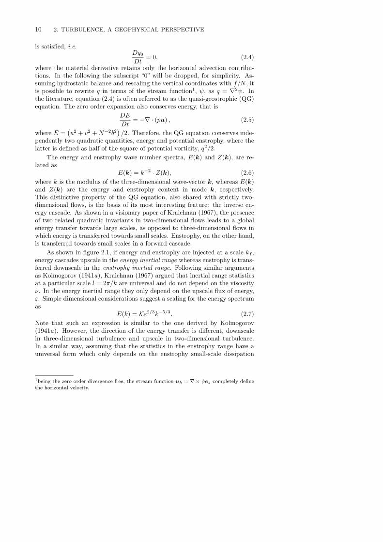
where k is the modulus of the three-dimensional wave-vector k, whereas E(k)and Z(k) are the energy and enstrophy content in mode k, respectively.This distinctive property of the QG equation, also shared with strictly two-dimensional flows, is the basis of its most interesting feature: the inverse en-ergy cascade. As shown in a visionary paper of Kraichnan (1967), the presenceof two related quadratic invariants in two-dimensional flows leads to a globalenergy transfer towards large scales, as opposed to three-dimensional flows inwhich energy is transferred towards small scales. Enstrophy, on the other hand,is transferred towards small scales in a forward cascade.

As shown in figure 2.1, if energy and enstrophy are injected at a scale kf ,energy cascades upscale in the energy inertial range whereas enstrophy is trans-ferred downscale in the enstrophy inertial range. Following similar argumentsas Kolmogorov (1941a), Kraichnan (1967) argued that inertial range statisticsat a particular scale l = 2(/k are universal and do not depend on the viscosity". In the energy inertial range they only depend on the upscale flux of energy,!. Simple dimensional considerations suggest a scaling for the energy spectrumas

E(k) = K!2/3k!5/3. (2.7)

Note that such an expression is similar to the one derived by Kolmogorov(1941a). However, the direction of the energy transfer is di!erent, downscalein three-dimensional turbulence and upscale in two-dimensional turbulence.In a similar way, assuming that the statistics in the enstrophy range have auniversal form which only depends on the enstrophy small-scale dissipation

1being the zero order divergence free, the stream function uh = "# $ez completely definethe horizontal velocity.

2.1. GEOSTROPHIC TURBULENCE 11

Figure 2.1. Sketch of the energy spectrum in two-dimensional and in QG turbulence (figure taken from Vallis2006).

leads to an energy spectrum of the form

E(k) = C#2/3k!3. (2.8)

The dimensionless constants, K and C, are assumed to be universal and areoften referred as Kraichnan and Kraichnan-Batchelor constant, respectively.The theory of Kraichnan (1967) has been tested numerically in a number ofstudies. Early investigations (Legras et al. 1988; Ohkitani 1990; Maltrud &Vallis 1993; Ohkitani & Kida 1992) indicated that the energy spectrum may besteeper in the enstrophy range as compared to Kraichnan’s prediction. How-ever, as computational resources allowed larger resolutions, (2.8) was recovered(Bo!etta 2007; Vallgren & Lindborg 2011). As for the enstrophy inertial range,recent high-resolution numerical simulations have confirmed the existence of aninverse energy cascade, even though a somewhat steeper spectrum than (2.7)has been obtained by some investigators. This steeper spectrum is likely tobe a result of formation of large scale coherent vortices (Scott 2007; Vallgren2011).

To what extent can the theory of QG turbulence explain large-scale at-mospheric and oceanic dynamics? Indeed, the inverse energy cascade of QGflows poses the question on how energy can be dissipated in rotating and strat-ified systems such as the Earth. Dissipation of kinetic and potential energycan only be achieved by means of molecular viscosity and di!usion which actat very small scales. In the atmosphere, for instance, these scales can be es-timated to be of the order of few centimetres or even millimetres. How toreconcile the picture of a large-scale inverse energy cascade dynamics with thepresence of small scale dissipation is a problem that has become increasingly


important as the resolution of numerical models has increased. Since QG dy-namics is not able to support a forward energy cascade, non-balanced motions,which do not satisfy the geostrophic and hydrostatic balance, must be takeninto account. How energy can be transferred from balanced quasi-geostrophicmotions to ageostrophic motions is a fundamental question that we attempt toanswer by means of high-resolution numerical simulations in Paper I and II.

2.2. Stratified turbulence

As flow scales decrease, the e!ects of rotation and stratification are reduced.In the atmosphere rotation becomes of secondary importance at scales of theorder of tens of kilometres. However, at such scales stratification is still veryimportant and typical Froude numbers are very small.

In the last decade there has been important advances in the understandingof turbulence in the presence of strong stratification. Thanks to novel numericalexperiments it has been possible to resolve the issue regarding the directionof the energy cascade in the strongly stratified regime. In the early worksit was suggested that strong stratification favours an inverse energy cascade.By rescaling the equations of motions as done by Riley et al. (1981), Lilly(1983) argued that strong stratification leads to the suppression of verticalmotions and a two-dimensionalisation of the flow. In this limit, an inversecascade would therefore be observed, as predicted by Kraichnan (1967). Lilly(1983) suggested that in the atmosphere energy in decaying three-dimensionalconvective turbulent patches would, due to the e!ect of the stable stratification,be transferred upscale and feed the growth of two-dimensional structures.

Despite the appeal of such a theory, advances in the understanding ofstrongly stratified turbulence in the last decade have proved that Lilly’s viewis wrong. In the limit of zero Fr, Billant & Chomaz (2001) showed that theNavier-Stokes equations allow for self-similar solutions with a vertical lengthscale lz " U/N , proposing an alternative scaling of the equations than the oneused by Lilly (1983) and Riley et al. (1981). Introducing di!erent vertical andhorizontal length scales, lz and lh respectively, and using the assumption ofhydrostatic balance, we can make the estimate: b " U2/lz and w " bU/N2lh "UlhFr2/lz. Thus, the following scalings for the advective terms should hold

u&

&x" U

lh, w

&

&z" Fr2

U lhl2z

" U

lh

Fr2

)2, (2.9)

where ) = lz/lh. Thus, if the estimate of Billant & Chomaz (2001) is usedfor lz, it follows that Fr " ) and the vertical component of the advectiveterm is of leading order and cannot be neglected as done in the analysis ofLilly (1983) and Riley et al. (1981). Billant & Chomaz (2001) introduced twodi!erent Froude numbers in their analysis, Fh and Fv, based on the horizontaland vertical length scales. Whereas Fh is a small quantity in strongly stratifiedturbulent flows, Fv always stays on the order of unity.

2.3. THREE-DIMENSIONAL TURBULENCE 13

Thus, a stratified system retains its intrinsic three-dimensionality and neverapproaches the two-dimensional manifold. Moreover, Billant & Chomaz (2000)showed that in stratified flows two-dimensional solutions are unstable with re-spect to a new type of instability, called the zig-zag instability, and thereforetend to become three-dimensional (Augier et al. 2013). The theoretical findingsof Billant & Chomaz (2001) have recently been confirmed in a number of nu-merical studies (Riley & deBruynKops 2003; Lindborg 2006; Waite & Bartello2006; Brethouwer et al. 2007; Augier et al. 2012). Riley & deBruynKops (2003)studied the decaying of Taylor-Green vortices numerically in strongly stratifiedmediums. They found that the suppression of vertical motions induced by thestable stratification provides a decoupling of layers, leading to large verticalgradients. From an initial condition where Fv & 1, Fv increases and becomesof the order of unity, allowing for Kelvin-Helmotz instabilities (KH) to develop.Indeed, KH provides a physical mechanism which allows for a transfer of energydownscale. Also box simulations of forced strongly stratified turbulence haveconfirmed that stratification favours a direct cascade (Lindborg 2006; Waite &Bartello 2006; Brethouwer et al. 2007). In agreement with the prediction ofLindborg (2006), the two-dimensional horizontal kinetic and potential energyspectra in the inertial range are found to scale as

EK(kh) = C1!2/3K k!5/3

h , EP (kh) = C2!P k!5/3h /!1/3K , (2.10)

where !K and !P represent the kinetic and potential energy dissipation. C1

and C2 are found to be of the order of unity and have similar values, i.e.C1 ' C2 = 0.51± 0.02 (Lindborg 2006). Using dimensional arguments, Billant& Chomaz (2001) suggested a scaling for the vertical energy spectrum

E(kz) = C N3 k!3z , (2.11)

with the dimensionless constant C being of the order of unity. As noted byBrethouwer et al. (2007), numerical and also experimental investigations ofstratified turbulence are very demanding in terms of Reynolds numbers. Itis only very recently that computational power has become strong enough torecover (2.11) in numerical simulations (Augier et al. 2012). In the inertialrange of the turbulent cascade, the e!ect of viscosity is supposedly negligible.However, at moderate Reynolds numbers, the constraint on the vertical lengthscale due to stratification leads to severe limitations. The viscous term relatedto the second order vertical derivative can be estimated as

"&2

&z2ui " "

U

l2z" "

U2

lh

Re

)=

U2

lh

1

ReFr2, (2.12)

which shows that the e!ective Reynolds number in stratified flows is reduced bya factor Fr2. Thus, even though Re is large, viscosity may a!ect the dynamicsif stratification is very strong.

2.3. Three-dimensional turbulence

As the scales of the flow reduce even further, also stratification becomes ofminor importance and classical three-dimensional Kolmogorov turbulence is


recovered. The transition between these two regimes is usually assumed to bethe so-called Ozmidov length scale, defined as (Ozmidov 1965)

lO =!1/2

N3/2, (2.13)

where ! is the energy flux towards small scales. The Ozmidov length scaleis usually interpreted as the largest scale at which overturning motions arepossible. Indeed, numerical simulations indicate that kO = 2(/lO is the wavenumber at which the energy spectrum shows a transition from a k!3 depen-dence, relation (2.11), to a k!5/3 dependence (Augier et al. 2012). Using theestimates of Billant & Chomaz (2001) and the estimate lh " u3/! (Lindborg2006), the following relations can be derived,

lhlO

" Fr!3/2 andlzlO

" Fr!1/2. (2.14)

The Ozmidoz length scale in the oceans has been estimated to be of the orderof metres (Gargett et al. 1981), whereas in the atmosphere, typical values mayvary between one metre, in strongly stratified atmospheric boundary layers(Frehlich et al. 2008), and ten metres, in the upper troposphere (Lindborg2006). At smaller scales, classical three dimensional turbulence develops andthe Kolmogorov (1941a) theory is valid. Vertical and horizontal energy spectrascale as

E(k) = C!2/3k!5/3, (2.15)

with a direct energy cascade from large to small scales. The Kolmogorov con-stant, C ' 1.6, is of the order of unity (Grant et al. 1962; Kaneda et al. 2003).Viscosity becomes important only at scales of the order of centimetres or evenmillimetres, where dissipation takes place.

2.4. Rotating turbulence

Even though rotating turbulence often appears in geophysical flows coupled tostratification, understanding how system rotation alone modifies the turbulentdynamics is very important. Rotating turbulence has been the subject of avast number of studies in the literature (e.g. Ibbetson & Tritton 1975; Cambonet al. 1997; Smith & Wale!e 1999; Moisy et al. 2011). Besides the geophysicalcontext, rotating turbulent also arises in a series of engineering problems, e.g.turbo-machinery. One of the most interesting features of flows subjected tosystem rotation is the presence of structures which are highly elongated in thedirection of the rotation vector ! (Taylor 1923; Hopfinger et al. 1982; Bartelloet al. 1994; Davidson et al. 2006). In the following, we will assume that !is aligned with the vertical axis z. If the rotation is strong, the leading-orderbalance in equation (2.1) is between the Coriolis term and the pressure gradient.The vertical component of the curl of (2.1) reduces to

f$h · u = f

$&u

&x+&v

&y

%= #f

&w

&z= 0, (2.16)

2.4. ROTATING TURBULENCE 15

where $h is the horizontal divergence operator. If we further assume thatthere is hydrostatic balance in the vertical direction, e.g. balance between thepressure term %!1&p/&z and the gravitational acceleration g, we find that alsothe vertical derivatives of u and v vanish in a constant density fluid. Thisis commonly referred to as Taylor-Proudman e!ect (Proudman 1916; Taylor1923).

In a slightly weaker form, the Taylor-Proudman e!ect means that rotat-ing flows are strongly anisotropic and exhibit very weak vertical gradients, i.e.vertically elongated structures develop. Columnar vortices have been observedin a number of experiments (Hopfinger et al. 1982; Davidson et al. 2006), eventhough the mechanisms underlying their formation are yet not fully under-stood (Wale!e 1993; Staplehurst et al. 2008). Davidson et al. (2006) showthat elongated structures grow in the vertical from an initial state of decay-ing three-dimensional turbulence when system rotation is applied. The growthrate of the vertical integral length scale was found to be proportional to therotation rate, lz " #t, suggesting that linear inertial wave can have a role onthe formation process of columnar structures (Staplehurst et al. 2008).

Indeed, waves are thought to have a crucial importance in the dynamics ofstrongly rotating flows (Wale!e 1993; Embid & Majda 1998). However, linearmechanisms cannot explain the transfer of energy towards large scales and thegrowth of the vertical integral length scale, which is an intrinsically nonlinearphenomenon. The two-time scale analysis of Embid & Majda (1998) suggeststhat, at large rotation rates, transfer of energy among scales is dominated bytriadic interactions of resonant waves (Wale!e 1993). Resonance takes placebetween three inertial waves which satisfy

k1 + k2 + k3 = 0 and *1 + *2 + *3 = 0, (2.17)

where ki is the wave vector and *i = fkz,i/ |ki| is the frequency of the i-th inertial wave. Cambon et al. (1997) showed that transfer of energy tendsto concentrate energy close to the plane kz = 0 (as also suggested by theinstability hypothesis of Wale!e 1993). This means that vertically elongatedstructures develop. Modes belonging to the plane kz = 0, for which * = 0,constitute, however, a closed resonant-set, meaning that energy into/out of thekz = 0 plane can only be transferred through o!-resonant triad interactions(Wale!e 1993). An intriguing question is whether purely 2D dynamics with aninverse energy cascade would be recovered as Ro ( 0 (Chen et al. 2005). Itis thought that two-dimensionalisation of the flow takes place through quasi-resonant triads, for which (2.17) is approximately satisfied only to a certaindegree (Cambon et al. 1997). On the other hand, it is worth pointing out thatthe analysis of Embid & Majda (1998) is built on the assumption that twoseparate time-scales exist in the flow: a slow advection time scale ta " L/U ,and a fast rotational time scale tw " * = fkz,i/ |ki|, for which tw & ta.However, as kz ( 0, the two time scales become similar and the analysis ofEmbid & Majda (1998) is likely to breakdown at kz/kh ' u/lhf = Ro (Belletet al. 2006), similar to what observed in stratified turbulence (Lindborg &


Brethouwer 2007) where a traditional two time-scales analysis breaks down atkh/kz " U/ (Nlh) = Fr.

The fact that vertically-elongated structures develop in rotating flowsposes severe limitations on experimental and numerical investigations of sucha regime. Boundary layer dynamics at solid walls together with the verticalexperimental confinement influence experiments conducted in rotating tanks(Ibbetson & Tritton 1975; Hopfinger & van Heijst 1993; Morize & Moisy 2006).In a similar way, numerical simulations can be a!ected by the choice of thevertical size of the computational domain, Lz. Numerical codes generally useperiodic boundary conditions in all three directions. The finite box height lim-its the lowest wave number which can be represented, k = 2(/Lz. Confining Lz

therefore prevents energy to be transferred to wave numbers that are smallerthan k. Recent studies of non-rotating unstratified turbulence have shown aninterestingly dynamics when the vertical size of the computational domain isreduced, where features of 3D and 2D turbulent dynamics mix and superim-pose (Celani et al. 2010). How this picture would change in the presence of asystem rotation is the subject of Paper IV.

2.4.1. Symmetry breaking in rotating flows

One intriguing aspect of rotating flows is that the Coriolis term breaks thereflectional invariance of the Navier-Stokes equations. A quantity is said to bereflectional invariant if it does not change under transformations which flip thedirection of one axis, e.g.

(x", y", z") ( (x, y,#z). (2.18)

Vectorial quantities should be referred to the appropriate system of reference,e.g.

(u", v", w") ( (u, v,#w). (2.19)

Equations (2.1) are clearly not invariant with respect to the transformation(2.18) and (2.19), because of the Coriolis term. As a consequence, positive andnegative vortical motions exhibit di!erent properties in rotating flows. Ex-periments in rotating tanks of barotropic vortices show completely di!erentflow evolution and patterns depending on the sign of the vorticity (van Heijst& Kloosterziel 1989; Hopfinger & van Heijst 1993). Motions with a positivevorticity with respect to the direction of the rotation vector are referred toas cyclonic, whereas motions with a negative vorticity are referred to as anti-cyclonic. A dominance of cyclonic motions has been observed in a number ofstudies of rotating turbulence, both in numerical simulations (Bartello et al.1994; Smith & Wale!e 1999) and experiments (Hopfinger et al. 1982; Moisyet al. 2011). One way of quantifying the breaking of symmetry is by meansof the skewness of the vorticity component parallel to the rotation rate vec-tor (Bartello et al. 1994):

S(*z) =)*3

z*)*2

z*3/2. (2.20)

2.5. TOWARDS THE ATMOSPHERE... 17

Gence & Frick (2001) showed that, if rotation is applied to a fully devel-oped isotropic three-dimensional turbulence, the numerator )*3

z* has a positivegrowth in time, thus giving evidence of a dominance of cyclonic motions duringthe transient spin-up process. Stability analysis may also provide an indicationof the dominance of cyclonic motions. The inviscid Rayleigh criterion in aninertial frame of reference suggests that barotropic cyclonic vortices are morestable than their anti-cyclonic counterparts, in agreement with the observations(Kloosterziel & van Heijst 1991). Sreenivasan & Davidson (2008) also foundthat the Ro threshold for blobs to evolve into columnar vortices is lower foranti-cyclonic motions, which are thus less likely to appear.

Even though several explanations have been proposed for the dominanceof cyclonic motions and this subject has been the object of an increasing atten-tion in recent years, the understanding of the symmetry breaking in rotatingturbulence is just“little more than a superficial cartoon” (Davidson et al. 2012).An intriguing question also concerns the limit of very strong rotation and strat-ification, discussed in §2.1. In this limit the Navier-Stokes equations reduce tothe QG equation, (2.4), which, interestingly, is parity-invariant. Thus, in theQG limit there can be no cyclonic/anti-cyclonic symmetry breaking.

Even though we are not able to o!er a new explanation in this thesis, weanyway address the symmetry breaking in rotating turbulence in Paper III andIV. We propose the use of an another quantity which may be of interest inplace of *z, that is the statistics of the azimuthal velocity di!erence )uT =t · (u (x+ r)# u (x)), where t is an horizontal unit vector perpendicular tothe separation vector r in the cyclonic direction. *z is in fact a small-scalequantity in three-dimensional turbulence, meaning that its value is dominatedby contributions at small-scales, and therefore a measure based on (2.20) maybe Re-dependent. On the other hand, statistics of )uT retain the dependenceon the separation scale r and can thus be more informative.

2.5. Towards the atmosphere...

Even though the separate turbulent regimes (three-dimensional, stratified andgeophysical turbulence) have been widely studied in the last decade, investi-gations of the transition from one dynamics to another are rather scarce. In-deed, within the context of numerical simulations, the available computationalresources impose severe constraints on the scale separations, and simulatingmore than one regime has not been possible until very recently.

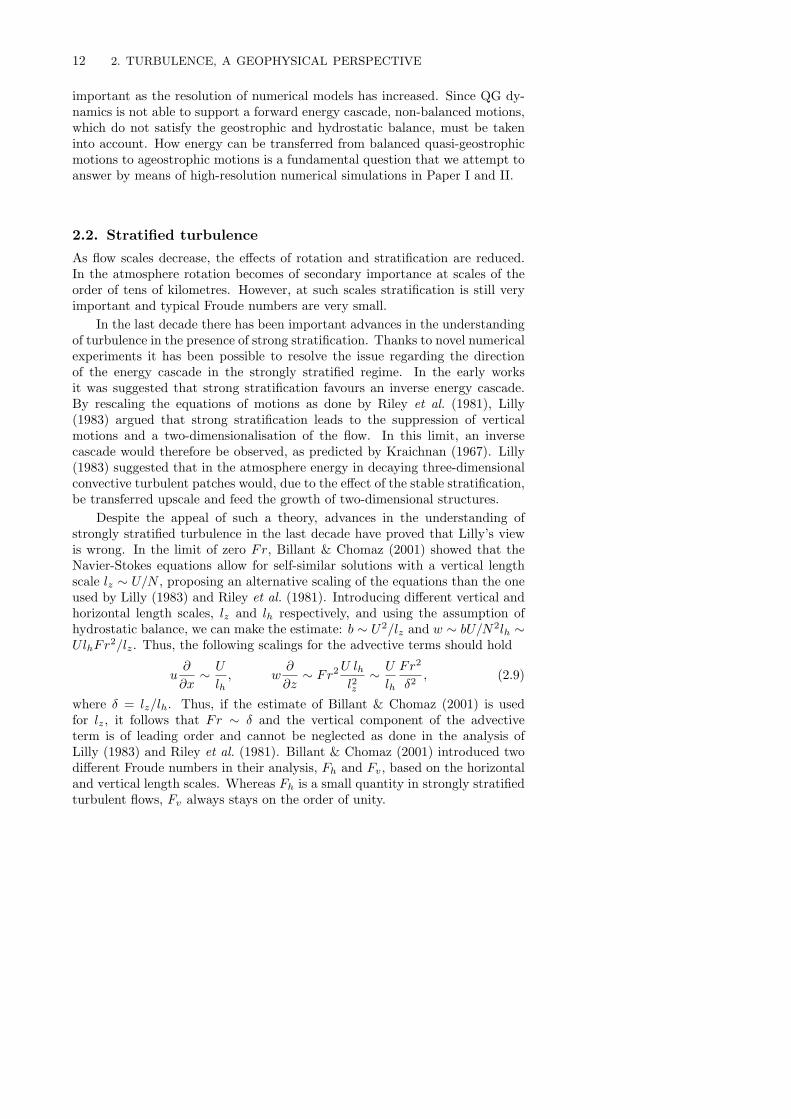
In order to shed light on atmospheric and oceanic dynamics, such investiga-tions are very important. One issue which is still an object of a vivid debate isthe so-called Nastom-Gage spectrum. By using sensors mounted in commercialaircraft, Nastrom et al. (1984) were able to measure the kinetic and potentialenergy spectra in the atmosphere from scales of the order of few kilometres upto scales of the order of thousand kilometres. The striking outcome of theirwork was the observation that the atmospheric energy spectrum clearly dividesinto two separate regimes (see figure 2.2): at synoptic scales (" 1000 km) a


Figure 2.2. Atmospheric spectra of kinetic energy of thezonal and meridional wind components and potential energymeasured by means of the potential temperature. The spectraof meridional wind and potential temperature are shifted oneand two decades to the right, respectively. Reproduced fromNastrom & Gage (1985).

spectrum of the form " k!3 is found, whereas at mesoscales (" 100 km) muchshallower spectra are observed, " k!5/3, with a smooth transition around 500km. More than twenty-five years later, it is still debated what dynamics areproducing these spectra.

While the k!3 range can be explained by a quasi-geostrophic turbulentdynamics, the k!5/3 range is more mysterious and intriguing, since such aspectrum may arise from both stratified and geostrophic turbulence (Vallis2006). However, the underlying dynamics is completely di!erent in the twocases, with a downscale cascade of energy in the former case and an upscalecascade of energy in the latter case. Early studies, e.g. Lilly (1983), interpretedthe k!5/3 range as a stratified upscale energy cascade. Nevertheless, recentprogress in stratified turbulence theory rather suggests that the k!5/3 range isa result of a downscale energy cascade. In spite of this, Lilly’s interpretationhas recently been revived by some experiments in electromagnetically forcedthick layers, suggesting that the presence of large-scale coherent vortices mightsuppress vertical motion and allow for an inverse cascade (Xia et al. 2011).


In order to determine the direction of the cascade in the k!5/3 range, otherstatistical quantities can be used in place of the energy spectrum. One suchquantity is the longitudinal third-order structure function,

))uL)u · )u* = )(uL (x+ r)# uL (x))

(u (x+ r)# u (x)) · (u (x+ r)# u (x))* , (2.21)

where uL is the velocity component parallel to r and )·* denotes the ensembleaverage. As opposed to the energy spectrum, the sign of ))uL)u · )u* di!ersdepending on the direction of the cascade, and therefore has been used to studythe atmospheric dynamics (Lindborg 1999; Cho & Lindborg 2001). In three-dimensional turbulence, an exact relation can be derived (Kolmogorov 1941b;Antonia et al. 1997),

))uL)u · )u* = #4

3!Kr. (2.22)

Its counterpart in two-dimensional turbulence was derived by Lindborg (1999)who found that ))uL)u · )u* is positive and has a cubic dependence in theenstrophy cascade range,

))uL)u · )u* = 1

4#r3, (2.23)

and a linear dependence in the energy cascade range,

))uL)u · )u* = 2Pr. (2.24)

Here, # is the enstrophy dissipation and P the energy injection rate. Analysesof the third-order structure functions calculated from measurements in thelower stratosphere (Cho & Lindborg 2001) have shown a positive nearly-cubicdependence at large scales, and a negative linear dependence at small scales,supporting the idea of a direct cascade of energy. Moreover, by using (2.23)and (2.24), Cho & Lindborg (2001) estimated the downscale enstrophy andenergy transfer2, which were found to be of the order of 2% 10!15 s!3 and 6%10!5 m2 s!2, respectively. However, it is questionable whether the use of (2.23)and (2.24), which were derived in the context of two-dimensional turbulence, isjustified, especially in the mesoscales. As suggested by the analysis of Billant& Chomaz (2001), vertical gradients may be important.

That the k!5/3 range can be explained by a direct energy cascade posesthe question where the energy feeding such a cascade could come from. Asnoted in the previous section, purely geostrophic dynamics is not consistentwith a downscale energy transfer. In order to investigate such a process, high-resolution numerical simulations are needed, able to resolve both geostrophicand stratified turbulent dynamics. In the last decade, several numerical studieshave been devoted to shed some lights into the dynamics, both using idealisedbox simulations (Kitamura & Matsuda 2006; Vallgren et al. 2011) and atmo-spheric models (Skamarock 2004; Takahashi et al. 2006; Hamilton et al. 2008;Waite & Snyder 2009).

2in equation (2.24) P is interpreted as the downscale energy flux


r

< δ

uL3 +

δ u

L δ u

T2 >

10−2 10−1 10010−5

10−4

10−3

10−2

10−1

100

r3

r

Ro

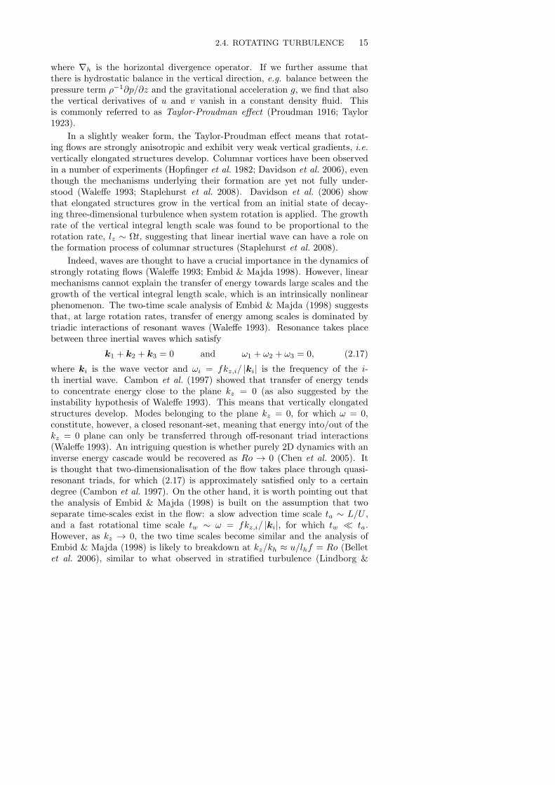
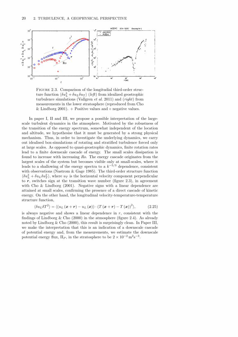
Figure 2.3. Comparison of the longitudial third-order struc-ture function ))u3

L+ )uL)uT * (left) from idealized geostrophicturbulence simulations (Vallgren et al. 2011) and (right) frommeasurements in the lower stratosphere (reproduced from Cho& Lindborg 2001). + Positive values and + negative values.

In paper I, II and III, we propose a possible interpretation of the large-scale turbulent dynamics in the atmosphere. Motivated by the robustness ofthe transition of the energy spectrum, somewhat independent of the locationand altitude, we hypothesise that it must be generated by a strong physicalmechanism. Thus, in order to investigate the underlying dynamics, we carryout idealised box-simulations of rotating and stratified turbulence forced onlyat large scales. As opposed to quasi-geostrophic dynamics, finite rotation rateslead to a finite downscale cascade of energy. The small scales dissipation isfound to increase with increasing Ro. The energy cascade originates from thelargest scales of the system but becomes visible only at small-scales, where itleads to a shallowing of the energy spectra to a k!5/3 dependence, consistentwith observations (Nastrom & Gage 1985). The third-order structure function))u3

L + )uL)u2T *, where uT is the horizontal velocity component perpendicular

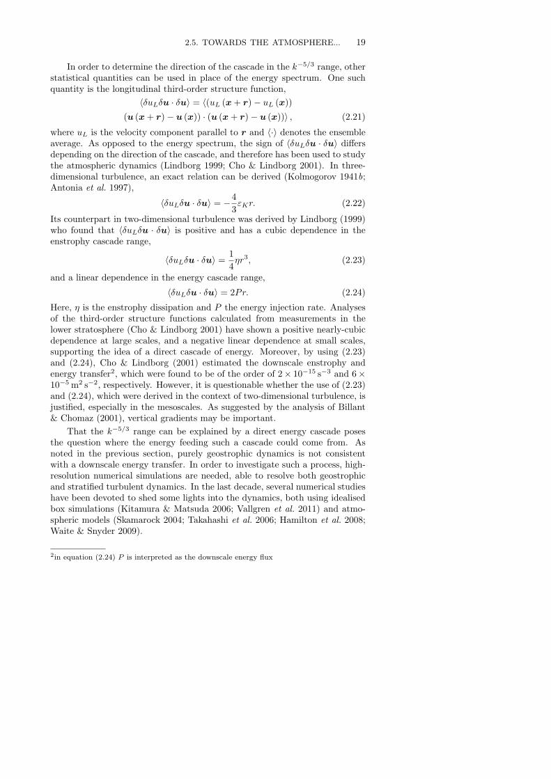
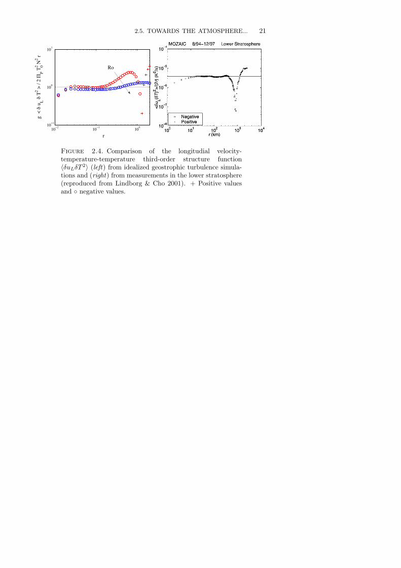
to r, switches sign at the transition wave number (figure 2.3), in agreementwith Cho & Lindborg (2001). Negative signs with a linear dependence areattained at small scales, confirming the presence of a direct cascade of kineticenergy. On the other hand, the longitudinal velocity-temperature-temperaturestructure function,

))uL)T2* = )(uL (x+ r)# uL (x)) · (T (x+ r)# T (x))2*, (2.25)

is always negative and shows a linear dependence in r, consistent with thefindings of Lindborg & Cho (2000) in the atmosphere (figure 2.4). As alreadynoted by Lindborg & Cho (2000), this result is surprisingly clean. In Paper III,we make the interpretation that this is an indication of a downscale cascadeof potential energy and, from the measurements, we estimate the downscalepotential energy flux, $P , in the stratosphere to be 2% 10!2 m2s!3.


r

g <

δ u

L δ T

2 > /

2 Π

P T02 N

2 r

10−2 10−1 10010−1

100

101

Ro

Figure 2.4. Comparison of the longitudial velocity-temperature-temperature third-order structure function))uL)T 2* (left) from idealized geostrophic turbulence simula-tions and (right) from measurements in the lower stratosphere(reproduced from Lindborg & Cho 2001). + Positive valuesand + negative values.

CHAPTER 3

Stratified and rotating turbulence in the presence ofwalls

Most flows in engineering applications and in nature develop over surfaces.From a practical point of view, the study of turbulence in the vicinity of asolid wall is therefore of essential importance. Early experimental investiga-tions (e.g. Reynolds 1886) were mainly devoted to wall-bounded turbulence.An inhomogeneous direction, normal to the wall1, substantially increases thecomplexity of the problem, as compared to the homogeneous case. From anumerical point of view, more complex numerical schemes and discretisationsare needed in order to deal with solid boundaries. It was only as late as in theend of the 80s that computational resources had reached a level that allowedfor wall-bounded turbulence simulations.

3.1. The scales of motions in wall-bounded turbulence

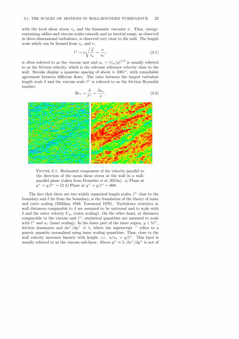
As in the isotropic homogeneous case, turbulent flows over solid walls possessmany scales. Figure 3.1 (taken from Deusebio et al. 2013a) shows a horizontalcomponent of the velocity in a wall-parallel plane close to the wall (figure 3.1a)and far from the wall (figure 3.1b). The turbulent dynamics is highly inhomoge-neous and very di!erent patterns are observed depending on the distance fromthe wall. In closed flows, such as channel or pipe flows, the largest turbulentlength scale is set by geometrical constraints, such as the channel height h orthe pipe diameter d. In boundary layers, on the other hand, where the flow isbounded at one side only, the largest scales are rather set by the boundary layerthickness. Away from the surface (figure b), a multitude of eddies of di!erentsize can be observed, with small-scale structures embedded in larger structures.Turbulence is close to be homogeneous and energy containing eddies are muchlarger than the scale at which energy is dissipated, which is of the order of the

local Kolmogorov length scale, # =""3/!

#1/4. Here, ! is the local dissipation

rate. On the other hand, figure 3.1b shows that close to the wall the dynamicsis dominated by a population of streamwise-elongated regions of high and lowvelocity. These small-scale structures, which are often referred to as streaks, arecommon to all turbulent flows developing over a solid surface. Their size scales

1hereafter denoted by y. The reader shall note that here we change the vertical axis from zto y in order to be consistent with the convention in wall-bounded turbulence studies, e.g.Spalart (1989).

22

3.1. THE SCALES OF MOTIONS IN WALL-BOUNDED TURBULENCE 23

with the local shear stress +w and the kinematic viscosity ". Thus, energy-containing eddies and viscous scales coincide and no inertial range, as observedin three-dimensional turbulence, is observed very close to the wall. The lengthscale which can be formed from +w and ",

l+ = "

&%

+w=

"

u!, (3.1)

is often referred to as the viscous unit and u! = (+w/%)1/2 is usually referred

to as the friction velocity, which is the relevant reference velocity close to thewall. Streaks display a spanwise spacing of about ' 100 l+, with remarkableagreement between di!erent flows. The ratio between the largest turbulentlength scale ) and the viscous scale l+ is referred to as the friction Reynoldsnumber,

Re! =)

l+=)u!

". (3.2)

Figure 3.1. Horizontal component of the velocity parallel tothe direction of the mean shear stress at the wall in a wall-parallel plane (taken from Deusebio et al. 2013a). a) Plane aty+ = y/l+ = 12 b) Plane at y+ = y/l+ = 800.

The fact that there are two widely separated length scales, l+ close to theboundary and ) far from the boundary, is the foundation of the theory of innerand outer scaling (Millikan 1938; Townsend 1976). Turbulence statistics atwall distances comparable to ) are assumed to be universal and to scale with) and the outer velocity U# (outer scaling). On the other hand, at distancescomparable to the viscous unit l+, statistical quantities are assumed to scalewith l+ and u! (inner scaling). In the lower part of the inner region, y < 5 l+,friction dominates and du+/dy+ ' 1, where the superscript + refers to ageneric quantity normalised using inner scaling quantities. Thus, close to thewall velocity increases linearly with height, i.e. u/u! = y/l+. This layer isusually referred to as the viscous sub-layer. Above y+ ' 5, du+/dy+ is not of

24 3. STRATIFIED AND ROTATING WALL TURBULENCE

the order of unity, although inner scaling still applies. This region is referred toas the bu!er layer. The two scalings match in an intermediate region (Millikan1938). In such a layer, the velocity gradient &u/&y must become independentof " and ), and scale only with u! and the distance from the wall y, i.e.&u/&y " u!/y. This leads to a logarithmic profile for the velocity,

u+ =1

,log y+ + C, (3.3)

where , is the von Karman constant. Figure 3.2 shows a prototype of thehorizontal velocity profile in wall-bounded flows. The di!erent regions, viscoussub-layer, bu!er layer, logarithmic region and outer layer can be observed. Eversince the discovery of the log-layer in wall-bounded flows, there has been a largedebate concerning whether there exists a true constant , which is universal toall wall-bounded flows. Indeed, results spanning several decades in Re num-bers, ranging from experiments (Osterlund et al. 2000; Monkewitz et al. 2007;Marusic et al. 2010), numerical simulations (Hoyas & Jimenez 2006; Schlatteret al. 2009; Spalart et al. 2009) and measurements in the atmosphere (Busingeret al. 1971; Andreas et al. 2006), have shown a relatively modest variation of,, ranging from 0.35 to 0.42. It is worth pointing out that these referencesare not exhaustive and they are only a very small part of the vast number ofstudies aimed at determining ,. An accurate description of this layer is, infact, of great practical interest, since most of the turbulent dissipation at highRe occurs in the log-layer.

Although the inner/outer scaling theory has been very successful in pre-dicting mean profiles, its applicability to higher moments is more questionable.In figure 3.3, the horizontal and vertical fluctuations scaled by u2

! are shown forseveral Re (Spalart et al. 2009; Deusebio et al. 2013a). Even very close to thewall, at y+ ' 12, the intensity of the near-wall peak located at y+ ' 12 doesnot collapse for the di!erent Re and it clearly increases with Re, suggestingthat there is a large-scale influence in the near-wall scaling. The variation ofthe maximum of urms with Re has received a great deal of attention in re-cent years and some empirical relations have been proposed, generally in thefunctional form of a logarithm (e.g. Marusic & Kunkel 2003). As shown byfigure 3.1, footprints of the large-scale structures can be seen close to the wall,suggesting that the outer structures penetrate deeply into the boundary layerand a!ect the near-wall turbulence scaling. Several studies have focused on theinteraction between large and small scales, involving spectral analysis (Hoyas& Jimenez 2006) as well as quantification of the small-scale modulations due tolarge scale structures (Schlatter & Orlu 2010; Mathis et al. 2011). In order tostudy such interactions a large separation of scales, and therefore a large Re,is desirable. Recent advancement in experimental techniques as well as newfacilities able to achieve extremely high Re will therefore provide extremelyvaluable data needed to study the interaction between outer and inner scalingsin wall-bounded flows (Hultmark et al. 2012; Marusic et al. 2013; Rosenberget al. 2013).

3.1. THE SCALES OF MOTIONS IN WALL-BOUNDED TURBULENCE 25

y+

(u2 +w2 )0.5

10−1 100 101 102 103 1040

5

10

15

20

25

Re

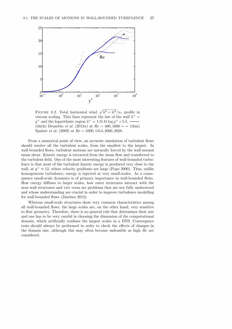
Figure 3.2. Total horizontal wind'u2 + w2/u! profile in

viscous scaling. Thin lines represent the law of the wall u+ =y+ and the logarithmic region u+ = 1/0.41 log y++5.5.(thick) Deusebio et al. (2013a) at Re = 400, 1600 (thin)Spalart et al. (2009) at Re = 1000, 1414, 2000, 2828.

From a numerical point of view, an accurate simulation of turbulent flowsshould resolve all the turbulent scales, from the smallest to the largest. Inwall-bounded flows, turbulent motions are naturally forced by the wall-normalmean shear. Kinetic energy is extracted from the mean flow and transferred tothe turbulent field. One of the most interesting features of wall-bounded turbu-lence is that most of the turbulent kinetic energy is produced very close to thewall, at y+ ' 12, where velocity gradients are large (Pope 2000). Thus, unlikehomogeneous turbulence, energy is injected at very small-scales. As a conse-quence small-scale dynamics is of primary importance in wall-bounded flows.How energy di!uses to larger scales, how outer structures interact with thenear-wall structures and vice versa are problems that are not fully understoodand whose understanding are crucial in order to improve turbulence modellingfor wall-bounded flows (Jimenez 2012).

Whereas small-scale structures show very common characteristics amongall wall-bounded flows, the large scales are, on the other hand, very sensitiveto flow geometry. Therefore, there is no general rule that determines their sizeand one has to be very careful in choosing the dimension of the computationaldomain, which artificially confines the largest scales in a DNS. Convergencetests should always be performed in order to check the e!ects of changes inthe domain size, although this may often become unfeasible as high Re areconsidered.


u rms/u

τ

y+10−1 100 101 102 103 1040

1

2

3

uh,rms

vrms

Figure 3.3. Total horizontal ( )'u"2 + w"2 and vertical

( )'v"2 profiles scaled with u! . Lines as in figure 3.2.

Arrows in the direction of increasing Re.

3.2. Numerical grids in wall-bounded flows

Since the first simulations in the 70s (Orszag & Patterson 1972), numericalsimulations of turbulent flows have heavily relied on the use of spectral methods(Canuto et al. 1988). As opposed to finite di!erence methods (FD) where thesolution is approximated on a finite grid, spectral methods (SM) approximatethe solution by using an expansion of known globally-defined ansatz functions.Instead of solving for the values at the grid points, spectral methods solvefor the expansion coe"cients. The only approximation which is introduced isthe truncation of the spectral expansion, whereas di!erential operators actingon the solution are exact. Due to the fact that a priori known functions arechosen, SM are not very flexible and only flows in fairly simple geometriescan be studied. However, as compared to the algebraic convergence of thesolution provided by finite di!erence methods, spectral methods allow for anexponential converge which had made them particularly useful, especially forturbulence simulations.

Several kind of ansatz functions can be used for the spectral expansion.The early studies of homogeneous isotropic turbulence (e.g. Orszag & Patterson1972) widely employed Fourier modes. Apart from the existence of fast trans-form algorithms (Fast Fourier Transforms, hereafter FFTs), Fourier modes alsohave the advantage of allowing for very simple formulations of partial di!er-ential equations since they are the eigenfunctions of the di!erential operator.

3.3. ROTATING WALL-BOUNDED FLOWS 27

However, for wall-bounded flows Fourier modes are not suitable in the wall-normal direction, due to the inhomogeneous boundary conditions and the needfor a non-equispaced grid (since wall structures are much finer as comparedto the outer ones). In the early numerical studies of wall-bounded turbulence,Chebyshev polynomials were instead used and applied to Gauss-Lobatto grids

yj/L = cos

$(j # 1

N # 1

%j = 1, · · · , N, (3.4)

which allowed both to retain the use of FFTs and to provide a non-uniformdistribution, with a clustering of points at the upper and lower boundaries,y = ±1. Such a grid is particularly suitable for flows confined by two solidwalls, e.g. channel flows. However, if one aims at studying open flows whichare bounded by only one solid wall, the clustering of points at the free-boundaryis a waste.

One way to overcome this problem is to use the method of Spalart et al.(2008) who employed Jacobi polynomials in the variable - = exp (#y/Y ), i.e.in a vertical grid exponentially stretched by a factor Y. Hoyas & Jimenez (2006)employed seven-point compact finite di!erences in place of the Chebyshev poly-nomials. In this way, they were able to adapt the grid spacing to the localviscous length scale #. Nevertheless, the employed solution algorithm still im-poses a clustering of points at the upper boundary. In paper VII, we proposean alternative method in order to study open flows which satisfy the upperboundary condition

&u

&y=&w

&y= v = 0, (3.5)

with u and w being the streamwise and spanwise velocities, respectively. Weretain the use of Chebyshev polynomials and the use of Gauss-Lobatto grids.However, we recast the study of open flows by considering flows which possesssymmetries around y = 0. The free-shear condition, when applied at y = 0, canin fact be viewed as a symmetric condition for u and w and an antisymmetriccondition for v. Thus, we can use only even Chebyshev polynomials in theexpansion of u and w, and only odd Chebyshev polynomials in the expansionof v. If vertical stratification is present, the scalar field must have the sameparity of the v equation and must therefore be odd. The spacing of the Gauss-Lobatto grid at y = 0 is coarse and the clustering of points at the free-shearboundary, now at y = 0, is thus avoided.

3.3. Rotating wall-bounded flows

Wall-bounded flows subjected to rotation around the vertical axis are veryimportant in a geophysical perspective. Indeed, the derivation of the solutionof a laminar rotating boundary layer of V. W. Ekman (1905) was inspired byobservations that in Arctic regions icebergs move with an angle of 30o#40o withrespect to the geostrophic wind (Nansen 1905). Far from the solid boundary,the main balance in the Navier-Stokes equations is between the Coriolis termand the pressure gradient, leading to the geostrophic balance #$p = %fey%G.


Here, ey is the wall-normal unit vector and G is the geostrophic wind vector.As the surface is approached, viscous shear stresses become of leading order.For a laminar parallel flow in steady conditions, the horizontal components ofthe Navier-Stokes equations reduce to

fw" = "&2u"

&x2and # fu" = "

&2w"

&z2, (3.6)

where the prime " indicates the fluctuation around the geosotrophic wind, u#G.If vanishing boundary conditions for the velocity u" are applied at infinity, i.e.

u", w" ( 0 as y ( ,, (3.7)

the system (3.6) admits self-similar solution with respect to the scaled verticalcoordinate y/)E , where )E =

'2"/f . In his landmark paper, Ekman (1905)

derived the solution to (3.6) and (3.7),

u" = Gx # e!y/#E {Gx cos (y/)E)#Gz sin (y/)E)}

w" = Gz # e!y/#E {Gx sin (y/)E) +Gz cos (y/)E)} .(3.8)

Ekman’s work (1905) had such an importance that boundary layers subjectedto a rotation around the vertical axis are nowadays referred to as Ekman layersin his honour. One of the most interesting features of the Ekman layer, incontrast to non-rotating boundary layers, is that the wind direction varies withheight. Figure 3.4 shows the odograph of the horizontal velocities, equation(3.8), which is usually referred to as the Ekman spiral. The wall shear-stresshas an angle of 45o with respect to the geostrophic wind direction, consistentwith the observation of Nansen (1905) that icebergs move in a direction whichis neither aligned with the geostrophic wind nor the oceanic current. It is worthpointing out that the condition (3.7) is rather demanding, especially in numer-ical simulations and experiments where the flow is usually confined verticallyby the height of the domain, Ly. By replacing the boundary conditions (3.7)with the free-shear condition (3.5), the solution to (3.6) has the form (Deusebioet al. 2013a)

u = +C1 cosh (y/)E) + C2 sinh (y/)E)

w = #C2 sinh (y/)E) + C1 cosh (y/)E) ,(3.9)

where the coe"cients C1 and C2 depend on the rescaled domain height, . =Ly/)E , as

C1 =#ug cosh. cos.# wg sinh. sin.

cosh2 . cos2 .+ sinh2 . sin2 .(3.10)

C2 =+ug sinh. sin.# wg cosh. cos.

cosh2 . cos2 .+ sinh2 . sin2 .. (3.11)

As .( ,, solution (3.9) exponentially converges to the Ekman solution (3.8).

Flows are very rarely laminar, especially in the atmosphere where the Ek-man Reynolds number, ReE = G)E/", is of the order of 106. As the flowbecomes turbulent, the Ekman spiral tends to shrink in the direction perpen-dicular to the geostrophic wind and the angle / between the wall shear-stress

3.3. ROTATING WALL-BOUNDED FLOWS 29

u/G

−w/G

0 0.2 0.4 0.6 0.8 1−0.1

0

0.1

0.2

0.3

0.4

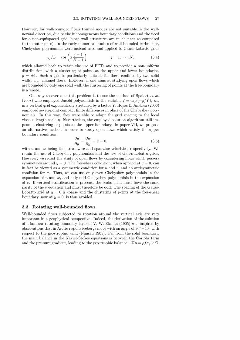
Figure 3.4. Ekman spiral for a laminar Ekman bound-ary layer and a turbulent Ekman boundary layer.

and the geostrophic wind consequently reduces (figure 3.4) as an e!ect of themore e"cient momentum transfer close to the wall (Coleman et al. 1990; Shin-gai & Kawamura 2002). Both in laminar and turbulent cases, the Ekmanspiral shows a small overshoot of the geostrophic wind velocity at intermediateheights, which can also be observed in the maximum of the velocity profileshown in figure 3.2. This is usually referred to as the low-level jet. It should bepointed out that it does not originate from an excess of momentum which dif-fuses vertically, as in common jets, but rather arises as an e!ect of the systemrotation.

An open question which is yet to be answered concerns the size and thenature of the largest structures of a turbulent Ekman boundary layer. In at-mospheric boundary layers, large-scale structures have been observed and theyare thought to be important on transport processes (Lemone 1973; Etling &Brown 1993). Experiments in a cylindrical annulus (Faller 1963; Faller & Kay-lor 1966; Tatro & Mollo-Christensen 1966) have also shown that large-scaleinstabilities develop. Stability analysis of the laminar Ekman solution (3.8)shows that there are two kinds of instabilities: a viscous parallel instabilityappearing at ReE = 55 and an inviscid instability arising for ReE > 115 as-sociated with inflectional points in the velocity profile (Faller & Kaylor 1966;Lilly 1966; Caldwell & Atta 1970). For both instabilities, the perturbationhas the form of rolling structures which have a negative inclination, for theparallel instability, and a positive inclination, for the inviscid instability, withrespect to the geostrophic wind (Lilly 1966). However, whether similar large-scale structures are also present in turbulent flows is an open question. EarlyDNSs of turbulent Ekman layers at ReE = 400 (Coleman et al. 1990) did notshow any evidence of large-scale roll cells, unless convective motions driven bya moderate heating of the lower surface were present in the flow (Coleman et al.1994). It is unclear whether the choice of the domain size may have prevented


Figure 3.5. Average 5o % 5o of the spin # " *y/2 (day!1,with sign reversed in the Southern hemisphere): cyclones (an-ticyclones) are indicated by blue, positive values (red, negativevalues). Figure taken from Gri!a et al. (2008).

their development. More recent flow visualisations of Ekman layers in DNSs atReE = 775 indicate that there are large-scale structures which are not alignedwith the direction of the geostrophic wind. Such structures were not observedin earlier DNSs (Shingai & Kawamura 2004). In paper V, we address the issueof large-scale structures in Ekman boundary layers at high ReE .

Rotating boundary layers present interesting di!erences with respect totheir non-rotating counterparts. As pointed out in §2.4.1, rotational termsbreak the parity invariance of the Navier-Stokes equations, as also observedfrom (3.6). Besides experiments and numerical simulations (see section §2.4.1),this symmetry breaking is also clearly seen in the large scale dynamics of theEarth atmosphere. Satellite images show that motions in low-pressure systemsare preferentially counter-clockwise in the northern hemisphere and clock-wisein the southern hemisphere. Preference for cyclonic or anticyclonic motions isobserved both in the atmosphere (Cho & Lindborg 2001) and in the oceans(see figure 3.5 taken from Gri!a et al. 2008). However, it is not obvious thatthe breaking of reflectional symmetry observed in large-scales atmospheric dy-namics can also be observed at smaller scales, for which Coriolis forces havea negligible e!ect. In this thesis, we present evidences that Ekman layers, incontrast to non-rotating boundary layers, can have a non-zero mean helicityand that a helicity cascade of a definite sign develops. We thus show that,as a consequence, the symmetry breaking can be observed down to the verysmallest scales of motions, the Kolmogorov length scale #, which is of the orderof one millimetre. Helicity, which is defined as the scalar product of velocityand vorticity

H = u · !, (3.12)

was first introduced by Mo!att (1969) who showed that it is an inviscidlyconserved quantity in a barotropic fluid, i.e. for which p = p(%). However,unlike energy and enstrophy, helicity does not have a definite sign and if the

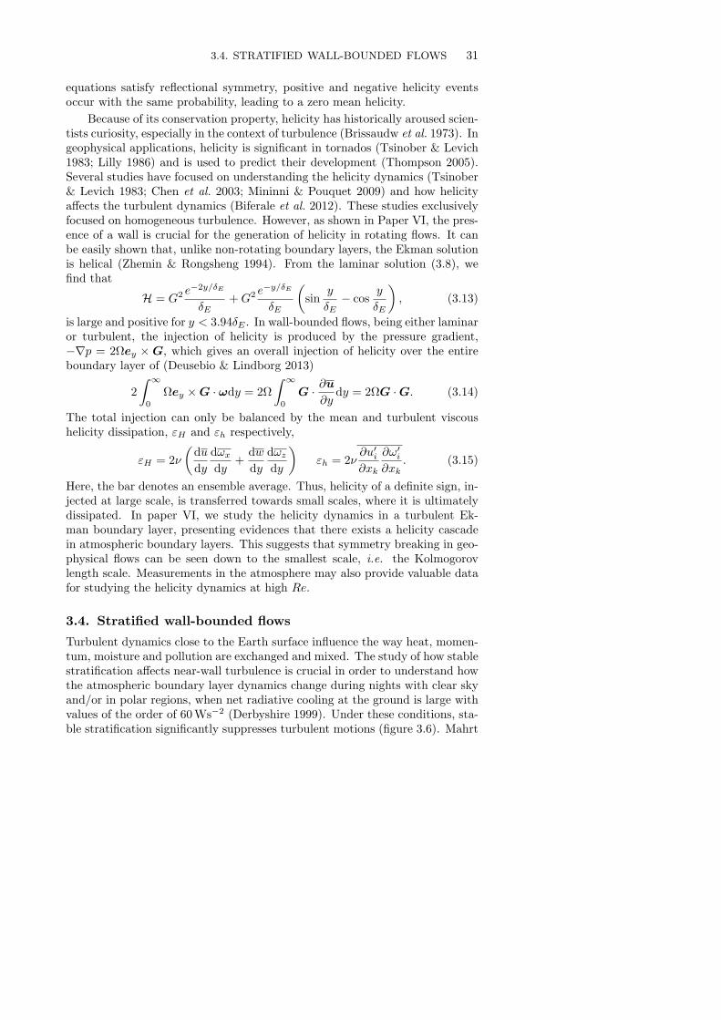
3.4. STRATIFIED WALL-BOUNDED FLOWS 31

equations satisfy reflectional symmetry, positive and negative helicity eventsoccur with the same probability, leading to a zero mean helicity.

Because of its conservation property, helicity has historically aroused scien-tists curiosity, especially in the context of turbulence (Brissaudw et al. 1973). Ingeophysical applications, helicity is significant in tornados (Tsinober & Levich1983; Lilly 1986) and is used to predict their development (Thompson 2005).Several studies have focused on understanding the helicity dynamics (Tsinober& Levich 1983; Chen et al. 2003; Mininni & Pouquet 2009) and how helicitya!ects the turbulent dynamics (Biferale et al. 2012). These studies exclusivelyfocused on homogeneous turbulence. However, as shown in Paper VI, the pres-ence of a wall is crucial for the generation of helicity in rotating flows. It canbe easily shown that, unlike non-rotating boundary layers, the Ekman solutionis helical (Zhemin & Rongsheng 1994). From the laminar solution (3.8), wefind that

H = G2 e!2y/#E

)E+G2 e

!y/#E

)E

$sin

y

)E# cos

y

)E

%, (3.13)

is large and positive for y < 3.94)E . In wall-bounded flows, being either laminaror turbulent, the injection of helicity is produced by the pressure gradient,#$p = 2#ey % G, which gives an overall injection of helicity over the entireboundary layer of (Deusebio & Lindborg 2013)

2

( #

0#ey %G · !dy = 2#

( #

0G · &u

&ydy = 2#G ·G. (3.14)

The total injection can only be balanced by the mean and turbulent viscoushelicity dissipation, !H and !h respectively,

!H = 2"

$du

dy

d*x

dy+

dw

dy

d*z

dy

%!h = 2"

&u"i

&xk

&*"i

&xk. (3.15)

Here, the bar denotes an ensemble average. Thus, helicity of a definite sign, in-jected at large scale, is transferred towards small scales, where it is ultimatelydissipated. In paper VI, we study the helicity dynamics in a turbulent Ek-man boundary layer, presenting evidences that there exists a helicity cascadein atmospheric boundary layers. This suggests that symmetry breaking in geo-physical flows can be seen down to the smallest scale, i.e. the Kolmogorovlength scale. Measurements in the atmosphere may also provide valuable datafor studying the helicity dynamics at high Re.

3.4. Stratified wall-bounded flows

Turbulent dynamics close to the Earth surface influence the way heat, momen-tum, moisture and pollution are exchanged and mixed. The study of how stablestratification a!ects near-wall turbulence is crucial in order to understand howthe atmospheric boundary layer dynamics change during nights with clear skyand/or in polar regions, when net radiative cooling at the ground is large withvalues of the order of 60Ws!2 (Derbyshire 1999). Under these conditions, sta-ble stratification significantly suppresses turbulent motions (figure 3.6). Mahrt


Figure 3.6. Figure taken from Banta et al. (2007). Timeseries of ground-level ozone (blue line, 1-min values in ppb)at Cornelia Fort Airpark, Nashville, Tennessee, for 15-22 Jul1999 (times UTC). Daytime hours are marked by the maximain O3 concentrations, and nights are the periods of mini- mumconcentrations. NO measurements (red line, ppb) availableafter 17 Jun document local-source activity at this site atnight.

(1998) divides the stable stratified boundary layer into two separate classesbased on their phenomenological characteristics: the weakly stable boundarylayer and the very stable boundary layer. The weakly stable boundary layer isrelatively well understood and is characterized by continuous turbulence whichis a!ected by buoyancy. On the other hand, the very stable boundary layer issomewhat more mysterious and less understood. Turbulence may be stronglydamped and virtually absent (Zilitinkevich et al. 2008) and occasional burstsof turbulence can also be observed (Kondo et al. 1978). Atmospheric mod-els need to be improved in order to take into account phenomena that arisein highly stably stratified conditions, as suppression of vertical motions, re-laminarisation and appearance of gravity waves. Numerical simulations canprovide an alternative tool, besides in-field measurements and experiments, tostudy the strongly stratified regime. This regime has recently been studied ina number of numerical investigations (e.g. Armenio & Sarkar 2002; Nieuwstadt2005; Flores & Riley 2010; Garcıa-Villalba & del Alamo 2011; Deusebio et al.2011).


For the weakly stable boundary layer, the so-called Monin-Obukhov simi-larity theory (Obukhov 1946; Monin & Obukhov 1954) has provided the founda-tion for our understanding of atmospheric flows, even for unstable stratification.The Monin-Obukhov similarity theory was introduced by Obukhov (1946) andMonin & Obukhov (1954) who proposed that in a region close to the surface,for which momentum and heat fluxes are approximately constant, statisticalquantities are only functions of the distance y from the surface, the frictionvelocity u! , the wall heat flux qw and the buoyancy parameter g/T0. UsingBuckingham (1914)’s theorem, dimensionless quantities are thus functions ofone independent dimensionless parameter: y/L, where L is the Monin-Obukhovlength given by

L = #u3!T0

,gqw. (3.16)

The von Karman constant , is historically included in the definition of L.According to (3.16), L is positive in stable conditions (qw < 0) and is negativein unstable conditions (qw > 0). When appropriately normalised, the meanvelocity gradient,

0m =,y

u!

&u

&y, (3.17)

and mean temperature gradient,

0h =,u!y

qw

&T

&y, (3.18)

shall therefore be universal functions of y/L. 0m and 0h are generally approx-imated by linear expressions y/L (see e.g. Monin et al. 1975),

0m) yL

*= 1 + Cm

y

Land 0h

) yL

*= 1 + Ch

y

L. (3.19)

As y/L ( 0, i.e. vanishing stratification, the log law (3.3) is recovered from(3.19). In very stable cases, Wyngaard (1973) argued that as a consequence ofsuppression of vertical motions, the wall distance y cannot enter into the Monin& Obukhov (1954) dimensional analysis. Thus, statistical quantities shouldbecome independent of y, e.g. 0m " y/L. Nieuwstadt (1984) and Holtslag &Nieuwstadt (1986) also proposed to extend the validity of the Monin-Obukhovsimilarity theory beyond the surface layer by considering a local version of Linstead, i.e. % = T0+3/2/gv"T ", where + and v"T " are the local turbulent shearstress and turbulent heat flux, respectively, at a certain height y. Observationsin the atmosphere (Businger et al. 1971; Kaimal et al. 1976; Nieuwstadt 1984;Metzger & Klewicki 2001) have shown a remarkable agreement with (3.19), bothin stable and unstable conditions. Recent numerical simulations at moderateRe have also confirmed the Monin-Obukhov theory for stably stratified flows,both with system rotation (Deusebio et al. 2013a) and without (Garcıa-Villalba& del Alamo 2011).

The Monin-Obukhov length scale L also o!ers an interesting physical in-terpretation. The wall-bounded turbulent dynamics of stratified flows is acompetition between the production of turbulent kinetic energy due to shear


and conversion to potential energy. L provides a measure of the relative im-portance of these two mechanisms. Assuming that the mean velocity followsthe log-law (3.3), the Monin-Obukhov length scale can be interpreted as thedistance at which the production,

u"v"&U

&y' u3

!

,y, (3.20)

and the turbulent kinetic to potential energy conversion,g

T0v"T " ' g

T0qw, (3.21)

are in balance.

At the wall, shear is generally very strong and dominates the dynamics.Even though the temperature/density gradients are sometimes largest at thewall, near-wall structures are little a!ected by stable stratification (Deuse-bio et al. 2011) and approximately preserve their spacing of ' 100 l+, alsoin strongly stratified continuously turbulent flows. An interesting question iswhat happens when stratification is so strong that the point y = L approachesthe near-wall region. If y = L provides an estimate of the height at which buoy-ancy becomes of leading order, then as L approaches the near-wall region, theentire boundary layer dynamics becomes buoyancy a!ected. For very strongstratification, continuously turbulence cannot be sustained, and portions of theflow relaminarise. Figure 3.7 shows the streamwise velocity (defined with re-spect to the shear stress at the wall) in a horizontal plane close to the wall foran Ekman layer at large stability (Deusebio et al. 2013a). Large portions ofthe flow undergo relaminarisation which appears in the form of inclined lam-inar bands. Thus, the flow exhibits strong spatial intermittency. For an evenstronger stratification, the inclined patterns further break down into turbulentspots. Similar inclined-bandy structures as the one shown in figure 3.7b have re-cently been observed in a number of studies of wall-bounded transitional flows,ranging from subcritical low-Re Couette flow (Prigent et al. 2002; Barkley &Tuckerman 2005; Duguet et al. 2010) to stratified open channel flow, rotatingCouette flow and magnetohydrodynamic channel flow (Brethouwer et al. 2012).However, the mechanisms underlying their formation and their dynamics arenot entirely clear (e.g. for a discussion about their inclination see Duguet &Schlatter 2013).

Several criteria for the onset of relaminarisation in strongly stratified flowshave been proposed, adopting non-dimensionless parameters such as the gradi-ent Richardson number (Miles 1961),

Ri =g

T0

&T

&y

$&u

&y

%!2

> 0.25, (3.22)

the flux Richardson number (Armenio & Sarkar 2002),

Ri =g

T0

v"T "

u"v"

$&U

&z

%!1

> 1, (3.23)


Figure 3.7. Instantaneous flow field of the streamwise veloc-ity component u in a wall parallel plane, at y+ ' 12. Fromleft to right stratification increases as: L+ ' 900, L+ ' 600and L+ ' 250. Taken from Deusebio et al. (2013a).

or the Nusselt number (Garcıa-Villalba & del Alamo 2011),

Nu =qwh

&T,T' 1 . (3.24)

Here, ,T is the kinematic di!usivity. More recent studies have proposed cri-teria based on the Monin-Obukhov length scale, L, rescaled by an outer scale(Nieuwstadt 2005) or the viscous length scale (Flores & Riley 2010). If wall-bounded turbulence is sustained by a near-wall cycle (e.g. Hamilton et al. 1995),inhibition of the near-wall dynamics by buoyancy forces can result in the globalrelaminarisation of the flow. Thus, it is likely that the criterion should involvenear-wall quantities (Flores & Riley 2010). As pointed out by de Wiel et al.(2012), when the flow is driven by external forces, e.g. a pressure gradient,a partial or total relaminarisation is followed by a flow acceleration. As a re-sult of larger shear stresses, turbulence can be triggered again and a globalintermittency can arise (Garcıa-Villalba & del Alamo 2011).

Ekman boundary layers are of great importance in geophysical flows andunderstanding how stratification a!ects their dynamics is crucial for many prac-tical applications. Before the development of computational power, the mainsource of data was, of course, observations. Even though measurements are ableto provide valuable data at very large Re, uncertainties of boundary conditionsand unstationarities pose severe limitation to their reliability. Numerical simu-lations o!er a new complementary tool to study stratified Ekman layers. Thefirst numerical simulations of an unstratified turbulent Ekman boundary layerswas shortly after followed by its stably (Coleman et al. 1992) and unstably(Coleman et al. 1994) counterparts. Shingai & Kawamura (2002) extendedthe study of Coleman et al. (1992) by investigating the structure of the Rey-nolds stresses and the heat fluxes. However, only very limited ReE , i.e. up toReE = 424, were considered. More recent numerical investigations have reliedon turbulence models in order to increase ReE (Taylor & Sarkar 2007, 2008b;Zilitinkevich & Esau 2007). However, caution should always be taken whenusing turbulence models to study strongly stratified flows. LESs significantly


underpredict turbulent transport processes in regions where the stratificationis strong and the vertical scales become small (Taylor & Sarkar 2008a). Ifnear-wall dynamics is crucial in the relaminarisation process, transitional flowsare also likely to be a!ected by the use of turbulence models. Therefore, DNSsremain the most accurate and trustworthy tool in the investigation of the sta-bly stratified boundary layer. However, recent progress in the understandingof strongly stratified regime in wall-bounded flows have not considered Ekmanboundary layers but have mainly focused to other flow cases (Nieuwstadt 2005;Garcıa-Villalba & del Alamo 2011; Brethouwer et al. 2012; Flores & Riley 2010;Deusebio et al. 2011), as channel and open-channel flows. In Paper V, we fillthis gap by carrying out a study of the Ekman boundary layer by means ofDNSs, ranging from unstratified conditions to very large stability.

CHAPTER 4

Summary of the papers

4.1. Homogeneous turbulence close to geostrophic conditions

We investigate the energy transfer in strongly stratified and rotating systemsin order to shed some light on the processes underlying the route to dissipationin geophysical flows. To this end, we carry out numerical simulations of homo-geneous turbulence in triply periodic domains forced only at large scales. Thehigh resolutions employed allow us to study more than one dynamical regimewithin the same simulations.

In paper I, we consider the so-called Primitive Equations, i.e. the Boussi-nesq system in which hydrostatic balance is assumed in the vertical, and weshow that two related cascade processes emanate from the same large scaleenergy source: a downscale cascade of potential enstrophy coexisting with adownscale energy cascade. We find that the amount of energy which is go-ing into the downscale energy cascade decreases monotonically with increasedrate of rotation and vanishes in the limit of Ro ( 0, reflecting the fact thatin quasi-geostrophic turbulence energy is transferred towards large scales. Atlarge scales the dynamics is dominated by a forward enstrophy cascade andenergy spectra scale as " k!3. The forward energy cascade, hidden at largescales, becomes visible only at smaller scales, where it leads to a shallowingof the spectra from " k!3 to " k!5/3. This is similar to observations in theatmosphere (Nastrom & Gage 1985), where a transition of kinetic and potentialenergy spectra from " k!3 to " k!5/3 is observed in the mesoscale range, atabout 500 kilometres.

In paper II, we extent the study to the full Boussinesq system, thus remov-ing the assumption of hydrostatic balance in the vertical direction. We showthat the Primitive Equations can be obtained from the Boussinesq equations bytaking the limit Fr2/Ro2 ( 0. When Fr2/Ro2 is small the di!erence betweenthe results from the BQ and the PE simulations is found to be small. We findthat larger degree of stratification favours a downscale energy cascade, eventhough the e!ect of stratification, within the range of parameters representa-tive for large-scale atmospheric dynamics, is weaker as compared to rotation indetermining the amount of energy going up- and down-scale. We further inves-tigate the dynamics by considering vertical spectra and we find that Charneyisotropy lz/lh " f/N is approximately valid at larger wave numbers than thethe transition wave number. We study the transfer of energy and enstrophy

37

38 4. SUMMARY OF THE PAPERS

throughout the turbulent cascade and find that, for intermediate degrees of ro-tation and stratification, a constant energy flux and a constant enstrophy fluxcoexist within the same range of scales. In this range, the enstrophy flux is aresult of triad interactions involving three geostrophic modes, while the energyflux is a result of triad interactions involving at least one ageostrophic mode,with a dominant contribution from interactions involving two ageostrophic andone geostrophic mode. The role of inertia-gravity waves is studied through anal-yses of time-frequency spectra of single Fourier modes. Only at large scales,distinct peaks at frequencies predicted for linear waves are observed, whereas atsmall scales no clear wave activity is observed, suggesting that wave dynamic isnegligible within the turbulent cascade. We further analyse the transfer termsand show that resonant-wave triadic interactions cannot explain the downscaleenergy transfer.

In Paper III, we study the third-order structure functions, focusing at acomparison with measurement in the lower stratosphere. In the range of scaleswith a downscale energy cascade of kinetic and available potential energy wefind that the third order structure functions display a negative linear depen-dence on separation distance r, in close agreement with the observations in theatmosphere. However, it is also found that terms including the vertical veloc-ity cannot be neglected when the energy flux is estimated. Estimates based onmeasured structure functions which only include the horizontal velocity com-ponent can therefore only provide an order of magnitude estimate of the energyflux. We also calculate the third order velocity structure functions that are notparity invariant and therefore display a cyclonic-anticyclonic asymmetry. Inclose agreement with the results from the stratosphere we find that these func-tions have an approximate r2-dependence, with strong dominance of cyclonicmotions.

In Paper IV, we discuss the e!ect of vertical confinement in homogeneousrotating turbulence. Vertical confinement is achieved by imposing the verticalperiodicity of the flow and by preventing energy to be transferred towards largervertical scales. Thus, boundary e!ects arising at solid walls are neglected. Inagreement with previous findings, we find that both confinement and rotationfavour an inverse energy cascade. However, we show that for moderate rotationrates the direct energy cascade can be recovered by vertically extending thecomputational box, i.e. reducing the lowest vertical wave number which canbe represented in the simulation.

4.2. Wall bounded stratified turbulence

As described in paper VII, an existing code, used to study turbulent channelflows, has been largely modified in order to e"ciently simulate flows which arebounded by one solid wall only, as for instance the Ekman boundary layer.The Gauss-Lobatto grid in the wall-normal direction, used in conjunction toa spectral discretisation based on Chebyshev polynomials, leads to a cluster-ing of points at the free boundary, which is superfluous in open flows since

4.2. WALL BOUNDED STRATIFIED TURBULENCE 39

turbulence is usually weak or non-existent at the upper boundary. By restrict-ing ourselves to flows with a free-shear surface, we note that equation (3.5)can be viewed as a symmetric conditions for u and w, and a anti-symmetriccondition for v at y = (y # Ly)/Ly = 0. Thus, we modify the numerical al-gorithm such that, depending on the considered variable, only one parity ofthe Chebyshev polynomials is retained. Since Gauss-Lobatto grids are coarserat y = 0, the clustering of points at the free-shear surface is avoided. In or-der to guarantee the speed-up of the code, an alternative formulation of theFast Fourier/Chebyshev transforms which accounts for the symmetry is pre-sented. Since we aim at carrying out direct numerical simulations at reasonablyhigh Reynolds numbers, the modifications have been implemented both in aone-dimensional (plane by plane) and two-dimensional (stencil) parallelisationstrategy. As an e!ect of the more e"cient discretisation, we show that thenumber of points in the vertical direction can be reduced, leading to an overallspeed-up of the code.

In paper V, we use this code to carry out a series of high-resolution nu-merical simulations of the turbulent Ekman layer at moderately high Rey-nolds number, 1600 < ReE < 3000. We present results for both neutrally,moderately and strongly stably stratified conditions. For unstratified cases,large-scale structures penetrating from the outer region down to the wall areobserved. These structures have a clear dominant frequency and can be re-lated to periodic oscillations or instabilities developing near the low-level jet.We investigate the e!ect of stratification and ReE on one-point and two-pointstatistics, focusing on the turbulent length scales. In the strongly stratifiedEkman layer we observe coexisting large-scale laminar and turbulent patchesappearing in the form of inclined bands, consistent with other wall-boundedflows. For weaker stratification, continuously sustained turbulence a!ected bybuoyancy is produced. We discuss the scaling of turbulent length scales, theheight of the Ekman layer, the friction velocity, the shear angle at the wall andthe heat flux. The boundary layer thickness, the friction velocity and the shearangle are shown to depend on Lf/u! , whereas the heat fluxes shows a betterscaling when plotted versus L+ = Lu!/".

The helicity dynamics in neutrally stratified Ekman boundary layers is in-vestigated in Paper VI. We define cyclonic and anticyclonic helicity with respectto the sign of ! ·eyH , where ! is the rotation vector and ey is the wall normalunit vector, positive for cyclonic helicity and negative for anticyclonic helicity.We find that there is a preference for cyclonic helicity in the lower part of theEkman layer and anticyclonic helicity in the uppermost part. We derive theevolution equations for the mean field helicity and the mean turbulent helicityand show that the pressure term injects cyclonic helicity at a rate 2#G2 overthe total depth of the Ekman layer, where G is the geostrophic wind far fromthe wall. A substantial part of the mean field helicity is transferred to turbulenthelicity which is ultimately destroyed by viscous e!ects. The helicity spectrum

40 4. SUMMARY OF THE PAPERS

displays a dependence close to " k!5/3 in an intermediate range of scales. Al-though the limited extent of this range prevents an accurate comparison withtheoretical predictions, results suggest the existence of a forward helicity cas-cade in the log-layer of Ekman boundary layers, as the one occurring in theatmosphere and oceans.

CHAPTER 5

Conclusions and outlook

Since their maturity, digital computers have allowed for a number of advances inthe understanding of turbulent processes. Their use have greatly increased overthe years and is expected to increase even further in the future. In this thesis, ithas been shown how numerical simulations can be used to study wall-boundedand homogeneous turbulence a!ected by stratification and rotation, allowingfor some insights into the atmospheric and oceanic turbulent dynamics.

5.1. Turbulence close to geostrophy: A key for improvingweather forecast...

We have analysed the dynamics in strongly stratified and rotating turbulenceby means of box simulations of homogeneous turbulence, ranging from the QGlimit to small but finite rotation rates and degrees of stratification. The use ofan idealised setup made it possible to study the backbone mechanism for theenergy transfer underlying rotating and stratified turbulence dynamics, free ofthe additional complexities present in measurements and global atmosphericmodels, such as topography, cloud dynamics, etc. Numerical simulations, al-though sometimes non-physical, allow to arbitrarily remove or separate thedi!erent contributions and to identify the key factors controlling the dynamics.

Unlike QG turbulence, where almost all turbulent energy cascades upscale,finite rotation rates lead to a leakage of energy towards small scales and, asa consequence, a forward energy cascade. This process can explain the exis-tence of a " k!5/3 range in the atmosphere, interpreted as a downscale energycascade range, and solve the apparent paradox of how and where dissipationcan take place in flows close to geostrophic conditions. Even though motionswhich are not in geostrophic balance are, at large scales, small compared tothe geostrophic motions, they have a crucial role in transferring the energydownscale. Great care should thus be taken in representing such motions inatmospheric models.

Despite the idealised setup, energy spectra and structure functions showremarkable agreement with measurements in the atmosphere, suggesting thatthe scenario of a hidden cascade emanating from the largest scales can explainthe observations. Recent analyses of data of global circulating models (GCMs)also show strong similarities with these findings (Augier & Lindborg 2013).One open question is whether such a process may occur also in the oceans.Indeed, observations are more di"cult and there is great uncertainty regarding

41

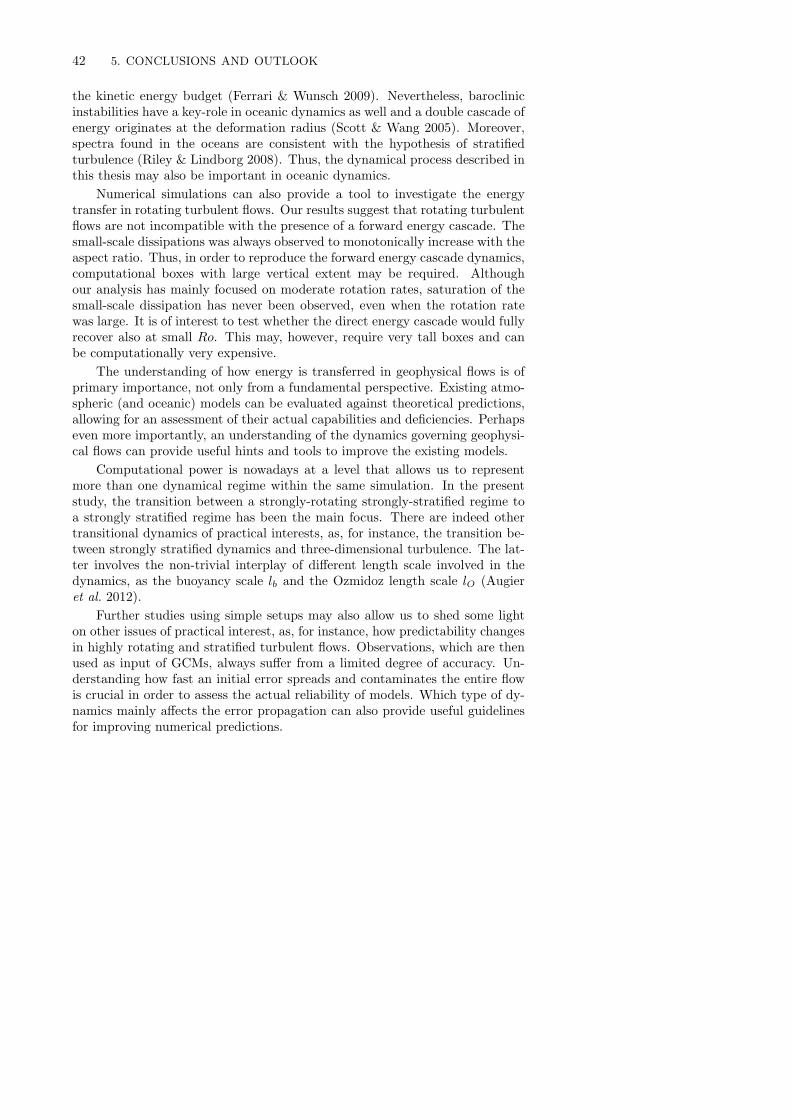
42 5. CONCLUSIONS AND OUTLOOK

the kinetic energy budget (Ferrari & Wunsch 2009). Nevertheless, baroclinicinstabilities have a key-role in oceanic dynamics as well and a double cascade ofenergy originates at the deformation radius (Scott & Wang 2005). Moreover,spectra found in the oceans are consistent with the hypothesis of stratifiedturbulence (Riley & Lindborg 2008). Thus, the dynamical process described inthis thesis may also be important in oceanic dynamics.

Numerical simulations can also provide a tool to investigate the energytransfer in rotating turbulent flows. Our results suggest that rotating turbulentflows are not incompatible with the presence of a forward energy cascade. Thesmall-scale dissipations was always observed to monotonically increase with theaspect ratio. Thus, in order to reproduce the forward energy cascade dynamics,computational boxes with large vertical extent may be required. Althoughour analysis has mainly focused on moderate rotation rates, saturation of thesmall-scale dissipation has never been observed, even when the rotation ratewas large. It is of interest to test whether the direct energy cascade would fullyrecover also at small Ro. This may, however, require very tall boxes and canbe computationally very expensive.

The understanding of how energy is transferred in geophysical flows is ofprimary importance, not only from a fundamental perspective. Existing atmo-spheric (and oceanic) models can be evaluated against theoretical predictions,allowing for an assessment of their actual capabilities and deficiencies. Perhapseven more importantly, an understanding of the dynamics governing geophysi-cal flows can provide useful hints and tools to improve the existing models.

Computational power is nowadays at a level that allows us to representmore than one dynamical regime within the same simulation. In the presentstudy, the transition between a strongly-rotating strongly-stratified regime toa strongly stratified regime has been the main focus. There are indeed othertransitional dynamics of practical interests, as, for instance, the transition be-tween strongly stratified dynamics and three-dimensional turbulence. The lat-ter involves the non-trivial interplay of di!erent length scale involved in thedynamics, as the buoyancy scale lb and the Ozmidoz length scale lO (Augieret al. 2012).

Further studies using simple setups may also allow us to shed some lighton other issues of practical interest, as, for instance, how predictability changesin highly rotating and stratified turbulent flows. Observations, which are thenused as input of GCMs, always su!er from a limited degree of accuracy. Un-derstanding how fast an initial error spreads and contaminates the entire flowis crucial in order to assess the actual reliability of models. Which type of dy-namics mainly a!ects the error propagation can also provide useful guidelinesfor improving numerical predictions.

5.2. THE ATMOSPHERIC BOUNDARY LAYER 43

5.2. Wall-bounded turbulence and atmospheric boundarylayers

We have carried out a series of direct numerical simulations of the Ekmanboundary layer, considering neutrally and stably stratified conditions. Thanksto the advancement in computational power, moderately high Reynolds num-ber could be simulated in computational boxes larger than what has been usedin previous studies. For neutrally stratified conditions, our results show thepresence of large-scale turbulent structure which has not been observed before,possibly prevented by the use of limited computational domains. It is not clearwhether such large-scale structures are of similar nature as the large-scale struc-tures observed in other wall-bounded flows. Our results show that they exhibita strong degree of coherency in the vertical direction and that their signaturescan be found close to the wall, therefore suggesting a significant influence onthe near-wall dynamics. The strong vertical coherency might also indicate thattheir origin is connected to a global instability of the flow. Ongoing work isaimed at studying the stability of the turbulent Ekman boundary layers inorder to verify such a conjecture.

Stable stratification was introduced in the flows by imposing a temperaturedi!erence in the vertical direction and its e!ect on the wall-bounded turbulentdynamics was investigated. For moderate degrees of stratification, statisticallysteady continuously turbulent states are observed. The height of the boundarylayer drastically reduces and it was shown to agree with theoretical predictions.Despite the limited Re, statistical quantities also showed reasonable agreementwith the Monin-Obukhov similarity theory in an intermediate range of scales.

On the other hand, when stratification is very strong the flow partially re-laminarises and laminar and turbulent motions coexist, similar to what is foundin other studies of transitional flows. The dynamics of laminar/turbulent pat-terns is, at current state, not fully understood and further studies should beaimed to better describe this regime. One open question concerns the conditionfor the appearance of laminar regions. In strongly stratified flows, our simula-tions show laminar patches already at L+ ' 500, thus larger than the criterionsuggested by Flores & Riley (2010) for open-channel flows, i.e. L+ ' 100.However, since only one moderately high Re was considered in the study, it isnot possible to assess whether the L+ criterion is appropriate and what shouldbe the actual value at which laminar regions appear. Although computation-ally expensive, reliable studies of the relaminarisation process should alwaysconsider boxes large enough to fit the presence of both laminar and turbulentpatches, as in the current study.

The database produced by numerical simulations gives a full knowledge ofthe flow, which can be very valuable. In the present context, it has been usedto study the helicily dynamics in atmospheric boundary layers (Deusebio &Lindborg 2013). It has been found that the Ekman boundary layer is highlyhelical and that a downscale helicity turbulent cascade exists within the loga-rithmic region. This remarkable result suggest that signatures of the breaking

44 5. CONCLUSIONS AND OUTLOOK

of parity invariance observed in large-scale geophysical flows are transferreddownscale to the smallest scale of motions of the flow, i.e. to the Kolmogorovscale. This new finding also opens the possibility of testing theories on thehelicity cascade at very large Reynolds numbers by means of measurementsin an atmospheric boundary layer, where Re is typically of the order of 106,unfeasible in numerical simulations.

Acknowledgments

This work is not only a doctoral thesis, but it is also - in my personal perspective- the logbook of a journey, of an adventure which has filled my life in the lastfour years. And, as any other journey, it would not have been possible withoutthe help of all the people I met along the way. Each one has, in a way oranother, contributed to it. Without you, this work (and this journey) wouldnot have been the same. Grazie!

In primis - my gratitude goes to my supervisor captain Erik Lindborg notonly for being my guide in this journey but, most of all, for trasmitting andsharing his tremendous passion for science and his romantic view of research. Ithas been an honour and a pleasure to be side by side in these years, which I willnever forget. Tack sa mycket! Every journey has a beginning. Mine startedwith an e-mail from Philipp Schlatter who I would like to personally thank forboth attracting me in Stockholm and for sharing, over the years, his knowledgeon numerics and simulations. I would like to thank Geert Brethouwer for all thefruitful discussions we had and for supporting me in my very first conference inRome. I wish to kindly thank Guido Bo!etta, for hosting me in Turin and forthe very many interesting discussions, not only on scientific matters. A specialthank goes to Anders Dahlkild who has kindly read and provided commentson this “logbook”.

Any success is not worth being lived if there is no one to share the happinesswith. And when some bad moments come, being a di"culty in the Phd or abroken elbow, it is important to have people that make you feel you are notalone. Andreas Vallgren and Pierre Augier, thanks for being great workmatesand good friends at the same time. Thank you Amin for being such a greatroom-mate over all these years. I wish you, Zeinab and Rayan-Zackaria allthe best on your new adventure, all together. A huge thank also goes to allthose people I had the luck to share my everyday life with: Nima, Daniel,Onofrio, Nicolo, Qiang, Gabriele, Zeinab, George, Ardheshir, Lailai, Armin,Joy, Taras, Werner, Iman, Francesco, Luca Brandt, Luca Biancofiore, Gaetano,Ruth, Azad, Cai-Juan, Igor, Peter, Marit, Krishna, Bernhard, Mihai, Timea,Walter, Reza, Ellinor, Karl, Christina and Heide. Ett sarskilt tack till Bubba fordin hjalp och ditt oandliga talamod med min svenska. Tristan, Valentina, Karin,

45

46 ACKNOWLEDGMENTS

Marta, Emmelie, Michele, Alessandro and Serena, thanks for the unforgettabletime here in Stockholm and for cheering me up in many many occasions. Iwould also like to thank Angela, Nic, Jean-An, Alex, Berghem and Lu, forbeing, despite the distance, always good friends I can count on.

But, in any journey, the most important thing is to never get lost. I wish todedicate this work to my cardinal points, to those stars that by shining brightin the sky always indicate the right direction.

Sara, thanks for always supporting me and believing in me, beyond any possiblehuman limit.

Mamma e Papa, grazie per esserci, sempre e comunque, per avere sempre tempoper ascoltare e per, nonostante i 2000 chilometri, farmi sempre sentire a casa.

La mezza e stata uno dei giorni piu belli qui a Stoccolma, grazie a Lorenzoper essere stato parte di quel giorno e di mille altri ricordi che, sopratutto neimomenti di di"colta, danno la forza ad andare avanti.

Un grazie particolare va infine a colei che ha ispirato ogni passo di questocammino, perche, di ogni passo, era la direzione. Grazie per essere stata, diquesto viaggio, la musa e la meta. Ti amo, Dada!

Bibliography

Andreas, E. L., Claffey, K. J., Jordan, R. E., Fairall, C. W., Guest, P. S.,Persson, P. O. G. & Grachev, A. A. 2006 Evaluations of the von Karmanconstant in the atmospheric surface layer. J. Fluid Mech. 559, 117–150.

Antonia, R. A., Ould-Rouis, M., Anselmet, F. & Zhu, Y. 1997 Analogy betweenpredictions of kolmogorov and yaglom. J. Fluid Mech. 332 (1), 395–409.

Armenio, V. & Sarkar, S. 2002 An investigation of stably stratified turbulentchannel flow using large-eddy simulation. J. Fluid Mech. 459, 1–42.

Augier, P., Billant, P. & Chomaz, J. M. 2013 Stratified turbulence forced withcolumnar dipoles. Numerical study. Submitted to J. Fluid Mech.

Augier, P., Chomaz, J. M. & Billant, P. 2012 Spectral analysis of the transitionto turbulence from a dipole in stratified fluid. J. Fluid Mech. 713, 86–108.

Augier, P. & Lindborg, E. 2013 A new formulation of the spectral energy budgetof the atmosphere, with application to two high-resolution general circulationmodels. J. Atmos. Sci. 70 (70), 2293–2308.

Banta, R. M., Mahrt, L., Vickers, D., Sun, J., Balsley, B. B., Pichugina,Y. L. & Williams, E. J. 2007 The very stable boundary layer on nights withweak low-level jets. J. Atmos. Sci. 64 (9), 3068–3090.

Barkley, D. & Tuckerman, L. S. 2005 Computational study of turbulent laminarpatterns in Couette flow. Phys. Rev. Lett. 94 (1), 014502.

Bartello, P., Metais, O. & Lesieur, M. 1994 Coherent structures in rotatingthree-dimensional turbulence. J. Fluid Mech. 273, 1–30.

Bellet, F., Godeferd, F. S., Scott, J. F. & Cambon, C. 2006 Wave turbulencein rapidly rotating flows. J. Fluid Mech. 562 (1), 83–121.

Benzi, R., Biferale, L. & Parisi, G. 1993 On intermittency in a cascade modelfor turbulence. Physica D: Nonlinear Phenomena 65 (1-2), 163–171.

Biferale, L., Musacchio, S. & Toschi, F. 2012 Inverse energy cascade in three-dimensional isotropic turbulence. Phys. Rev. Lett. 108 (16), 164501.

Biferale, L. & Toschi, F. 2001 Anisotropic homogeneous turbulence: Hierarchyand intermittency of scaling exponents in the anisotropic sectors. Phys. Rev.Lett. 86, 4831–4834.

Billant, P. & Chomaz, J.-M. 2000 Experimental evidence for a new instability ofa vertical columnar vortex pair in a strongly stratified fluid. J. Fluid Mech. 418,167–188.

47

48 BIBLIOGRAPHY

Billant, P. & Chomaz, J.-M. 2001 Self-similarity of strongly stratified inviscidflows. Phys. Fluids 13 (6), 1645–1651.

Boffetta, G. 2007 Energy and enstrophy fluxes in the double cascade of two-dimensional turbulence. J. Fluid Mech. 589, 253–260.

Boussinesq, J. 1877 Essai sur la the’orie des eaux courantes. Imprimerie nationale- J. sav. 1’Acad. des Sci. .

Brethouwer, G., Billant, P., Lindborg, E. & Chomaz, J.-M. 2007 Scalinganalysis and simulation of strongly stratified turbulent flows. J. Fluid Mech.585, 343–368.

Brethouwer, G., Duguet, Y. & Schlatter, P. 2012 Turbulent–laminar coex-istence in wall flows with Coriolis, buoyancy or Lorentz forces. J. Fluid Mech.704, 137.

Brissaudw, A., Frisch, U., Leorat, J., Lesieur, M. & Mazure, A. 1973 Helicitycascades in fully developed isotropic turbulence. Phys. Fluids 16, 1366.

Buckingham, E. 1914 On physically similar systems; illustrations of the use of di-mensional equations. Phys. Rev. 4 (4), 345–376.

Businger, J., Wyngaard, J. C., Izumi, Y. & Bradley, E. F. 1971 Flux-profilerelationships in the atmospheric surface layer. J. Atmos. Sci. 28 (2), 181–189.

Caldwell, D. R. & Atta, C. W. V. 1970 Characteristics of Ekman boundary layerinstabilities. J. Fluid Mech. 44 (1), 79–95.

Cambon, C., Mansour, N. N. & Godeferd, F. S. 1997 Energy transfer in rotatingturbulence. J. Fluid Mech. 337, 303–332.

Canuto, C., Hussaini, M. Y., Quarteroni, A. & Zang, T. A. 1988 Spectralmethods in Fluid Dynamics. Springer-Verlag.

Celani, A., Musacchio, S. & Vincenzi, D. 2010 Turbulence in more than two andless than three dimensions. Phys. Rev. Lett. 104 (18), 184506.

Charney, J. G. 1971 Geostrophic turbulence. J. Atmos. Sci. 28 (6), 1087–1094.

Chen, Q., Chen, S., Eyink, G. L. & Holm, D. D. 2003 Intermittency in the jointcascade of energy and helicity. Phys. Rev. Lett. 90 (21), 214503.

Chen, Q., Chen, S., Eyink, G. L. & Holm, D. D. 2005 Resonant interactions inrotating homogeneous three-dimensional turbulence. J. Fluid Mech. 542, 139–164.

Cho, J. Y. N. & Lindborg, E. 2001 Horizontal velocity structure functions in theupper troposphere and lower stratosphere: 1. observations. J. Geophys. Res.106 (D10), 10223–10232.

Coleman, G. N., Ferziger, J. H. & Spalart, P. R. 1990 A numerical study ofthe turbulent Ekman layer. J. Fluid Mech. 213, 313–348.

Coleman, G. N., Ferziger, J. H. & Spalart, P. R. 1992 Direct simulation of thestably stratified turbulent Ekman layer. J. Fluid Mech. 244 (1), 677–712.

Coleman, G. N., Ferziger, J. H. & Spalart, P. R. 1994 A numerical study ofthe convective boundary layer. Boun.-Lay. Meteorol. 70 (3), 247–272.

Davidson, P. A., Kaneda, Y. & Sreenivasan, K. R. 2012 Ten Chapters in Tur-bulence. Cambridge University Press.

Davidson, P. A., Staplehurst, P. J. & Dalziel, S. B. 2006 On the evolution ofeddies in a rapidly rotating system. J. Fluid Mech. 557 (1), 135–144.

Deardorff, J. W. 1970 A numerical study of three-dimensional turbulent channelflow at large Reynolds numbers. J. Fluid Mech. 41, 453–480.

BIBLIOGRAPHY 49

Del Alamo, J. C., Jimenez, J., Zandonade, P. & Moser, R. D. 2006 Self-similarvortex clusters in the turbulent logarithmic region. J. Fluid Mech. 561, 329–358.

Derbyshire, S. H. 1999 Boundary-layer decoupling over cold surfaces as a physicalboundary-instability. Boun.-Lay. Meteorol. 90 (2), 297–325.

Deusebio, E., Brethouwer, G., Schlatter, P. & Lindborg, E. 2013a A numer-ical study of the unstratified and stratified Ekman layer. Submitted to J. FluidMech. .

Deusebio, E. & Lindborg, E. 2013 Helicity in the Ekman boundary layer. Submittedto J. Fluid Mech.

Deusebio, E., Schlatter, P., Brethouwer, G. & Lindborg, E. 2011 Direct nu-merical simulations of stratified open channel flows. J. Phys.: Conf. Ser. 318 (2),022009.

Deusebio, E., Vallgren, A. & Lindborg, E. 2013b The route to dissipation instrongly stratified and rotating flows. J. Fluid Mech. 720, 66–103.

Domaradzki, J. A. & Saiki, E. M. 1997 A subgrid-scale model based on the esti-mation of unresolved scales of turbulence. Phys. Fluids 9 (7), 2148–2164.

Duguet, Y. & Schlatter, P. 2013 Oblique laminar-turbulent interfaces in planeshear flows. Phys. Rev. Lett. 110 (3), 034502.

Duguet, Y., Schlatter, P. & Henningson, D. S. 2010 Formation of turbulentpatterns near the onset of transition in plane Couette flow. J. Fluid Mech. 650,119.

Ekman, V. W. 1905 On the influence of the Earth’s rotation on ocean currents. Arch.Math. Astron. Phys. 2, 1–52.

Embid, P. F. & Majda, A. J. 1998 Low Froude number limiting dynamics for stablystratified flow with small or finite Rossby numbers. Geophys. Astro. Fluid Dyn.87 (1-2), 1–50.

Etling, D. & Brown, R. A. 1993 Roll vortices in the planetary boundary layer: Areview. Boun.-Lay. Meteorol. 65 (3), 215–248.

Faller, A. J. 1963 An experimental study of the instability of the laminar Ekmanboundary layer. J. Fluid Mech. 15 (163), 560–576.

Faller, A. J. & Kaylor, R. E. 1966 A numerical study of the instability of thelaminar Ekman boundary layer. J. Atmos. Sci. 23, 466–480.

Ferrari, R. & Wunsch, C. 2009 Ocean Circulation Kinetic Energy: Reservoirs,Sources, and Sinks. Ann. Rev. Fluid Mech. 41, 253–282.

Feynman, R. P. 1964 Feynman lectures on physics. Addison-Wesley.

Flores, O. & Riley, J. J. 2010 Analysis of turbulence collapse in stably stratifiedsurface layers using direct numerical simulation. Boun.-Lay. Meteorol. 129 (2),241–259.

Frehlich, R., Meillier, Y. & Jensen, M. L. 2008 Measurements of boundarylayer profiles with in situ sensors and doppler lidar. J. Atmos. Oceanic Tech. 25,1328.

Frisch, U. 1996 Turbulence. Cambridge University Press.

Garcıa-Villalba, M. & del Alamo, J. C. 2011 Turbulence modification by stablestratification in channel flow. Phys. Fluids 23 (4), 045104.

Gargett, A. E., Hendricks, P. J., Sanford, T. B., Osborn, T. R. & Williams,A. J. 1981 A composite spectrum of vertical shear in the upper ocean. J. Phys.Oceanogr. 11, 1258–1271.

50 BIBLIOGRAPHY

Gatski, T. B. & Speziale, C. G. 1993 On explicit algebraic stress models forcomplex turbulent flows. J. Fluid Mech. 254, 59–78.

Gence, J. N. & Frick, C. 2001 Naissance des correlations triples de vorticite dansune turbulence statistiquement homogene soumise a une rotation. Comptes Ren-dus de l’Academie des Sciences-Series IIB-Mechanics 329 (5), 351–356.

Germano, M. 1992 Turbulence - The filtering approach. J. Fluid Mech. 238, 325–336.

Germano, M., Piomelli, U., Moin, P. & Cabot, W. H. 1991 A dynamic subgrid-scale eddy viscosity model. Phys. Fluids 3 (7), 1760–1765.

Gill, A. E. 1982 Atmosphere-ocean dynamics. Academic Press, New York.

Grant, H. L., Stewart, R. W. & Moilliet, A. 1962 Turbulence spectra from atidal channel. J. Fluid Mech. 12 (2), 241–268.

Griffa, A., Lumpkin, R. & Veneziani, M. 2008 Cyclonic and anticyclonic motionin the upper ocean. Geophys. Res. Lett. 35 (1), L01608.

Hamilton, J. H., Kim, J. & Waleffe, F. 1995 Regeneration mechanisms of near-wall turbulence structures. J. Fluid Mech. 287, 317–348.

Hamilton, K., Takahashi, Y. O. & Ohfuchi, W. 2008 Mesoscale spectrum of at-mospheric motions investigated in a very fine resolution global general circulationmodel. J. Geophys. Res. 113 (18).

van Heijst, G. J. F. & Kloosterziel, R. C. 1989 Tripolar vortices in a rotatingfluid pp. 569–571.

Holtslag, A. A. M. & Nieuwstadt, F. T. M. 1986 Scaling the atmospheric bound-ary layer. Boun.-Lay. Meteorol. 36 (1-2), 201–209.

Hopfinger, E. J., Browand, F. K. & Gagne, Y. 1982 Turbulence and waves in arotating tank. J. Fluid Mech. 125, 505–534.

Hopfinger, E. J. & van Heijst, G. J. F. 1993 Vortices in rotating fluids. Ann.Rev. Fluid Mech. 25 (1), 241–289.

Hoyas, S. & Jimenez, J. 2006 Scaling of the velocity fluctuations in turbulent chan-nels up to Re! = 2003. Phys. Fluids 18 (1), 011702.

Hultmark, M., Vallikivi, M., Bailey, S. C. C. & Smits, A. J. 2012 Turbulentpipe flow at extreme Reynolds numbers. Phys. Rev. Lett. 108 (9), 094501.

Ibbetson, A. & Tritton, D. J. 1975 Experiments on turbulence in a rotating fluid.J. Fluid Mech. 68 (04), 639–672.

Jimenez, J. 2012 Cascades in wall-bounded turbulence. Ann. Rev. Fluid Mech. 44,27–45.

Kaimal, J. C., Wyngaard, J. C., Haugen, D. A., Cote, O. R., Izumi, Y.,Caughey, S. J. & Readings, C. J. 1976 Turbulence structure in the convectiveboundary layer. J. Atmos. Sci. 33 (11), 2152–2169.

Kaneda, Y., Ishihara, T., Yokokawa, M., Itakura, K. & Uno, A. 2003 En-ergy dissipation rate and energy spectrum in high resolution direct numericalsimulations of turbulence in a periodic box. Phys. Fluids 15 (2), L21–L24.

Kim, J., Moin, P. & Moser, R. 1987 Turbulence statistics in fully developed channelflow at low Reynolds number. J. Fluid Mech. 177, 133–166.

Kitamura, Y. & Matsuda, Y. 2006 The k"3H and k"5/3

H energy spectra in stratifiedturbulence. Geophys. Res. Lett. 33, L05809.

Kloosterziel, R. C. & van Heijst, G. J. F. 1991 An experimental study ofunstable barotropic vortices in a rotating fluid. J. Fluid Mech 223 (1).

BIBLIOGRAPHY 51

Kolmogorov, A. N. 1941a Dissipation of energy in locally isotropic turbulence [InRussian]. Dokl. Akad. Nauk SSSR 32, 19–21.

Kolmogorov, A. N. 1941b The local structure of turbulence in incompressible vis-cous fluid for very large Reynolds numbers [In Russian]. Dokl. Akad. Nauk SSSR30, 299–303.

Kondo, J., Kanechika, O. & Yasuda, N. 1978 Heat and momentum transfersunder strong stability in the atmospheric surface layer. J. Atmos. Sci. 35 (6),1012–1021.

Kraichnan, R. H. 1967 Inertial ranges in two-dimensional turbulence. Phys. Fluids10 (7), 1417–1423.

Legras, B., Santangelo, P. & Benzi, R. 1988 High-resolution numerical experi-ments for forced two-dimensional turbulence. Europhys. Lett. 5, 37.

Lemone, M. A. 1973 The structure and dynamics of horizontal roll vortices in theplanetary boundary layer. J. Atmos. Sci. 30 (6), 1077–1091.

Lilly, D. K. 1966 On the instability of Ekman boundary flow. J. Atmos. Sci. 23 (5),481–494.

Lilly, D. K. 1983 Stratified turbulence and the mesoscale variability of the atmo-sphere. J. Atmos. Sci. 40 (3), 749–761.

Lilly, D. K. 1986 The structure, energetics and propagation of rotating convectivestorms. Part II: Helicity and storm stabilization. J. Atmos. Sci. 43 (2), 126–140.

Lindborg, E. 1999 Can the atmospheric kinetic energy spectrum be explained bytwo-dimensional turbulence? J. Fluid Mech. 388, 259–288.

Lindborg, E. 2006 The energy cascade in a strongly stratified fluid. J. Fluid Mech.550, 207–242.

Lindborg, E. & Brethouwer, G. 2007 Stratified turbulence forced in rotationaland divergent modes. J. Fluid Mech. 586, 83–108.

Lindborg, E. & Cho, J. Y. N. 2000 Determining the cascade of passive scalarvariance in the lower stratosphere. Phys. Rev. Lett. 85 (26), 5663.

Lindborg, E. & Cho, J. Y. N. 2001 Horizontal velocity structure functions in theupper troposphere and lower stratosphere: 2. theoretical considerations. Journalof Geophysical Research: Atmospheres (1984–2012) 106 (D10), 10233–10241.

Lorenz, E. N. 1963 Deterministic nonperiodic flow. J. Atmos. Sci. 20, 130–148.

Mahrt, L. 1998 Nocturnal boundary-layer regimes. Boun.-Lay. Meteorol. 88 (2),255–278.

Maltrud, M. E. & Vallis, G. K. 1993 Energy and enstrophy transfer in numericalsimulations of two-dimensional turbulence. Phys. Fluids 5, 1760–1775.

Marusic, I. & Kunkel, G. J. 2003 Streamwise turbulence intensity formulation forflat-plate boundary layers. Phys. Fluids 15, 2461.

Marusic, I., McKeon, B. J., Monkewitz, P. A., Nagib, H. M., Smits, A. J.& Sreenivasan, K. R. 2010 Wall-bounded turbulent flows at high Reynoldsnumbers: Recent advances and key issues. Phys. Fluids 22, 065103.

Marusic, I., Monty, J. P., Hultmark, M. & Smits, A. J. 2013 On the logarithmicregion in wall turbulence. J. Fluid Mech. 716, R3.

Mathis, R., Marusic, I., Hutchins, N. & Sreenivasan, K. R. 2011 The rela-tionship between the velocity skewness and the amplitude modulation of thesmall scale by the large scale in turbulent boundary layers. Phys. Fluids 23 (12),121702–121702.

52 BIBLIOGRAPHY

Metzger, M. M. & Klewicki, J. C. 2001 A comparative study of near-wall tur-bulence in high and low Reynolds number boundary layers. Phys. Fluids 13,692.

Miles, J. W. 1961 On the stability of heterogeneous shear flows. J. Fluid Mech.10 (4), 496–508.

Millikan, C. B. 1938 A critical discussion of turbulent flows in channels and circulartubes. In Proc. 5th Int. Congr. Appl. Mech, pp. 386–392.

Mininni, P. D. & Pouquet, A. 2009 Helicity cascades in rotating turbulence. Phys.Rev. E 79 (2), 026304.

Moffatt, H. K. 1969 The degree of knottedness of tangled vortex lines. J. FluidMech. 35 (1), 117–129.

Moin, P. & Mahesh, K. 1998 Direct numerical simulation: a tool in turbulenceresearch. Ann. Rev. Fluid Mech. 30 (1), 539–578.

Moisy, F., Morize, C., Rabaud, M. & Sommeria, J. 2011 Decay laws, anisotropyand cyclone–anticyclone asymmetry in decaying rotating turbulence. J. FluidMech. 666, 5–35.

Monin, A. A. S., Yaglom, A. M. & Lumley, J. L. 1975 Statistical Fluid Mechanics:Mechanics of Turbulence, , vol. 2. MIT Press.

Monin, A. S. & Obukhov, A. M. 1954 Basic laws of turbulent mixing in the surfacelayer of the atmosphere. Contrib. Geophys. Inst. Acad. Sci. USSR 151, 163–187.

Monkewitz, P. A., Chauhan, K. A. & Nagib, H. M. 2007 Self-consistent high-Reynolds-number asymptotics for zero-pressure-gradient turbulent boundarylayers. Phys. Fluids 19, 115101.

Morize, C. & Moisy, F. 2006 Energy decay of rotating turbulence with confinemente!ects. Phys. Fluids 18 (6), 065107–065107.

Moser, R. D. & Moin, P. 1987 The e!ects of curvature in wall-bounded turbulentflows. J. Fluid Mech. 175, 479–510.

Nansen, F. 1905 The Norwegian North polar expedition, 1893-1896: Scientific re-sults. Longmans, Green and Company.

Nastrom, G. D. & Gage, K. S. 1985 A climatology of atmospheric wavenumberspectra of wind and temperature observed by commercial aircraft. J. Atmos. Sci.42, 950–960.

Nastrom, G. D., Gage, K. S. & Jasperson, W. H. 1984 Kinetic energy spectrumof large-and mesoscale atmospheric processes. Nature 310 (5972), 36–38.

Nieuwstadt, F. T. M. 1984 The turbulent structure of the stable, nocturnal bound-ary layer. J. Atmos. Sci. 41 (14), 2202–2216.

Nieuwstadt, F. T. M. 2005 Direct numerical simulation of stable channel flow atlarge stability. Boun.-Lay. Meteorol. 116, 277–299.

Obukhov, A. M. 1946 Turbulence in the atmosphere with inhomogeneous tempera-ture. Trudy geofiz. inst. AN SSSR 1.

Ohkitani, K. 1990 Nonlocality in a forced two-dimensional turbulence. Phys. Fluids2 (9), 1529–1531.

Ohkitani, K. & Kida, S. 1992 Triad interactions in a forced turbulence. Phys. Fluids4 (4), 794–802.

Orszag, S. A. & Patterson, G. S. 1972 Numerical simulation of three-dimensionalhomogeneous isotropic turbulence. Phys. Rev. Lett. 28, 76–79.

BIBLIOGRAPHY 53

Osterlund, J. M., Johansson, A. V., Nagib, H. M. & Hites, M. H. 2000 A noteon the overlap region in turbulent boundary layers. Phys. Fluids 12 (1), 1.

Ozmidov, R. V. 1965 On the turbulent exchange in a stably stratified ocean. Izv.Acad. Sci. USSR, Atmos. Oceanic Phys. 1, 493–497.

Pedlosky, J. 1987 Geophysical Fluid Dynamics. Springer.

Pope, S. B. 2000 Turbulent flows. Cambridge university press.

Prigent, A., Gregoire, G., Chate, H., Dauchot, O. & van Saarloos, W. 2002Large-scale finite-wavelength modulation within turbulent shear flows. Phys.Rev. Lett. 89 (1), 6465.

Proudman, J. 1916 On the motion of solids in a liquid possessing vorticity. Proc.Roy. Soc. London 92 (642), 408–424.

Rasam, A., Brethouwer, G., Schlatter, P., Li, Q. & Johansson, A. V. 2011E!ects of modelling, resolution and anisotropy of subgrid-scales on large eddysimulations of channel flow. J. Turb. p. N10.

Reynolds, O. 1886 On the theory of lubrication and its application to Mr.Beauchamp Tower’s experiments, including an experimental determination ofthe viscosity of olive oil. Philos. Trans. R. Soc. Lond., I 177, 157–234.

Reynolds, O. 1895 On the dynamical theory of incompressible viscous fluids and thedetermination of the criterion. Philos. Trans. R. Soc. Lond., A 186, 123–164.

Reynolds, W. C. 1990 The potential and limitations of direct and large eddy sim-ulations. In Whither Turbulence? Turbulence at the Crossroads, , vol. 357, pp.313–343.

Richardson, L. F. 1922 Weather Prediction by Numerical Process. Dover Publica-tions, Inc., New York.

Riley, J. J. & deBruynKops, S. M. 2003 Dynamics of turbulence strongly influ-enced by buoyancy. Phys. Fluids 15 (7), 2047–2059.

Riley, J. J. & Lindborg, E. 2008 Stratified turbulence: A possible interpretationof some geophysical turbulence measurements. J. Atmos. Sci. 65 (7), 2416–2424.

Riley, J. J., Metcalfe, R. W. & Weissman, M. A. 1981 Direct numerical simula-tions of homogeneous turbulence in density-stratified fluids. AIP Conf. Proceed.76 (1), 79–112.

Rosenberg, B. J., Hultmark, M., Vallikivi, M., Bailey, S. C. C. & Smits,A. J. 2013 Turbulence spectra in smooth-and rough-wall pipe flow at extremereynolds numbers. J. Fluid Mech. 731, 46–63.

Schlatter, P. & Orlu, R. 2010 Assessment of direct numerical simulation data ofturbulent boundary layers. J. Fluid Mech. 659 (1), 116–126.

Schlatter, P., Orlu, R., Li, Q., Brethouwer, G., Fransson, J. H. M., Jo-hansson, A. V., Alfredsson, P. H. & Henningson, D. S. 2009 Turbulentboundary layers up to Re" = 2500 studied through simulation and experiment.Phys. Fluids 21 (5), 051702.

Scott, R. B. & Wang, F. 2005 Direct evidence of an oceanic inverse kinetic energycascade from satellite altimetry. J. Phys. Oceanogr. 35 (9), 1650–1666.

Scott, R. K. 2007 Nonrobustness of the two-dimensional turbulent inverse cascade.Phys. Rev. E 75, 046301.

Segalini, A., Orlu, R., Schlatter, P., Alfredsson, H. P., Ruedi, J.-D. &Talamelli, A. 2011 A method to estimate turbulence intensity and transverse

54 BIBLIOGRAPHY

Taylor microscale in turbulent flows from spatially averaged hot-wire data. Exp.Fluids 51, 693–700.

Shingai, K. & Kawamura, H. 2002 Direct numerical simulation of turbulent heattransfer in the stably stratified Ekman layer. Therm. Sci. Eng. 10, 25.

Shingai, K. & Kawamura, H. 2004 A study of turbulence structure and large-scalemotion in the Ekman layer through direct numerical simulations. J. Turb. 5 (1).

Sillero, J. A., Jimenez, J. & Moser, R. D. 2013 One-point statistics for turbulentwall-bounded flows at Reynolds numbers up to !+ ! 2000. Phys. Fluids 25,105102.

Skamarock, W. C. 2004 Evaluating mesoscale NWP models using kinetic energyspectra. Mon. Weather Rev. 132 (12), 3019–3032.

Smagorinsky, J. 1963 General circulation experiments with the primitive equations.Mon. Weather Rev. 91, 99.

Smith, L. M. & Waleffe, F. 1999 Transfer of energy to two-dimensional large scalesin forced, rotating three-dimensional turbulence. Phys. Fluids 11, 1608.

Spalart, P. R. 1988 Direct simulation of a turbulent boundary layer up to Re" =1410. J. Fluid Mech. 187, 61–98.

Spalart, P. R. 1989 Theoretical and numerical study of a three-dimensional turbu-lent boundary layer. J. Fluid Mech. 205, 319–340.

Spalart, P. R., Coleman, G. N. & Johnstone, R. 2008 Direct numerical simula-tion of the Ekman layer: A step in Reynolds number, and cautious support fora log law with a shifted origin. Phys. Fluids 20, 101507.

Spalart, P. R., Coleman, G. N. & Johnstone, R. 2009 Retraction: “Directnumerical simulation of the Ekman layer: A step in Reynolds number, andcautious support for a log law with a shifted origin”. Phys. Fluids 21 (10),109901.

Sreenivasan, B. & Davidson, P. A. 2008 On the formation of cyclones and anti-cyclones in a rotating fluid. Phys. Fluids 20, 085104.

Staplehurst, P. J., Davidson, P. A. & Dalziel, S. B. 2008 Structure formationin homogeneous freely decaying rotating turbulence. J. Fluid Mech. 598 (1),81–105.

Stolz, S. & Adams, N. A. 1999 An approximate deconvolution procedure for large-eddy simulation. Phys. Fluids 11 (7), 1699–1701.

Takahashi, Y. O., Hamilton, K. & Ohfuchi, W. 2006 Explicit global simulation ofthe mesoscale spectrum of atmospheric motions. Geophys. Res. Lett. 33, L12812.

Tatro, P. R. & Mollo-Christensen, E. L. 1966 Experiments on Ekman layerinstability. PhD thesis, Cambridge Univ Press.

Taylor, G. I. 1923 Experiments on the motion of solid bodies in rotating fluids.Proc. R. Soc. Lond., A 104, 213–218.

Taylor, J. R. & Sarkar, S. 2007 Internal gravity waves generated by a turbulentbottom Ekman layer. J. Fluid Mech. 590, 331–354.

Taylor, J. R. & Sarkar, S. 2008a Direct and large eddy simulations of a bottomEkman layer under an external stratification. Int. J. of Heat and Fluid Flow29 (3), 721–732.

Taylor, J. R. & Sarkar, S. 2008b Stratification e!ects in a bottom Ekman layer.J. Phys. Oceanogr. 38 (11), 2535–2555.

Thompson, R. 2005 Explanation of spc severe weather parameters.

Townsend, A. A. 1976 The Structure of Turbulent Shear Flow . Cambridge Univer-sity Press.

Tsinober, A. & Levich, E. 1983 On the helical nature of three-dimensional coherentstructures in turbulent flows. Phys. Lett. A 99 (6), 321–324.

Vallgren, A. 2011 Infrared Reynolds number dependency of the two-dimensionalinverse energy cascade. J. Fluid Mech. 667, 463–473.

Vallgren, A., Deusebio, E. & Lindborg, E. 2011 A possible explanation of theatmospheric kinetic and potential energy spectra. Phys. Rev. Lett. 99, 99–101.

Vallgren, A. & Lindborg, E. 2011 The enstrophy cascade in forced two-dimensional turbulence. J. Fluid Mech. 671, 168–183.

Vallis, G. K. 2006 Atmospheric and Oceanic Fluid Dynamics: Fundamentals andLarge-scale Circulation; electronic version. Leiden: Cambridge Univ. Press.

Waite, M. L. & Bartello, P. 2006 The transition from geostrophic to stratifiedturbulence. J. Fluid Mech. 568, 89–108.

Waite, M. L. & Snyder, C. 2009 The mesoscale kinetic energy spectrum of abaroclinic life cycle. J. Atmos. Sci. 66, 883.

Waleffe, F. 1993 Inertial transfers in the helical decomposition. Phys. Fluids 5, 677.

de Wiel, B. J. H. V., Moene, A. F. & Jonker, H. J. J. 2012 The cessation ofcontinuous turbulence as precursor of the very stable nocturnal boundary layer.J. Atmos. Sci. 69 (11), 3097–3115.

Wyngaard, J. C. 1973 On surface-layer turbulence. Workshop in Micrometeorologypp. 101–149, Boston.

Xia, H., Byrne, D., Falkovich, G. & Shats, M. 2011 Upscale energy transfer inthick turbulent fluid layers. Nat. Phys. 7 (4), 321–324.

Zhemin, T. & Rongsheng, W. 1994 Helicity dynamics of atmospheric flow. Adv.Atmos. Sci. 11 (2), 175–188.

Zilitinkevich, S. S., Elperin, T., Kleeorin, N., Rogachevskii, I., Esau, I.,Mauritsen, T. & Miles, M. W. 2008 Turbulence energetics in stably stratifiedgeophysical flows: Strong and weak mixing regimes. Quart. J. Roy. Meteor. Soc.134 (633), 793–799.

Zilitinkevich, S. S. & Esau, I. 2007 Similarity theory and calculation of turbulentfluxes at the surface for the stably stratified atmospheric boundary layer. Boun.-Lay. Meteorol. 125 (2), 193–205.

Numerical studies in rotating and stratified turbulence

Documents

Transcript of Numerical studies in rotating and stratified turbulence